Slide 1Lecture 12 6.837 Fall ‘01

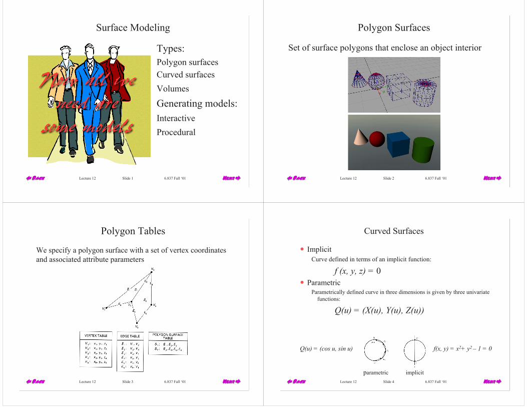
Surface Modeling

Types: Polygon surfacesCurved surfacesVolumes

Generating models: Interactive Procedural

Slide 2Lecture 12 6.837 Fall ‘01

Polygon Surfaces

Set of surface polygons that enclose an object interior

Slide 3Lecture 12 6.837 Fall ‘01

Polygon Tables

We specify a polygon surface with a set of vertex coordinates and associated attribute parameters

Slide 4Lecture 12 6.837 Fall ‘01

Curved Surfaces

� ImplicitCurve defined in terms of an implicit function:

f (x, y, z) = 0� Parametric

Parametrically defined curve in three dimensions is given by three univariate functions:

Q(u) = (X(u), Y(u), Z(u))

Q(u) = (cos u, sin u) f(x, y) = x2+ y2 – 1 = 0

parametric implicit

Slide 5Lecture 12 6.837 Fall ‘01

Implicit vs. Parametric

Surface Display�Parametric

Surface Intersections� Implicit

Changing Topology� Implicit

1 2( , , ) ( , , ) 0f x y z f x y z− =

Slide 6Lecture 12 6.837 Fall ‘01

Parametric Example: Beziér Curves

We can generate points on the curve by repeated linear interpolation.Starting with the control polygon (in red), the edges are subdivided (as noted in blue). These points are then connected in order and the resulting edges subdivided. The recursion stops when only one edge remains. This allows us to approximate the curve at multiple resolutions.

A Beziér curve can be defined in terms of a set of control points denoted in red.Consider, for example, a cubic, or curve of degree 3:

3 20 1

2 32 3

( ) (1 ) 3 (1 )

3 (1 )

Q u u p u u pu u p u p

= − + −

+ − +

Slide 7Lecture 12 6.837 Fall ‘01

Beziér Patches

Control polyhedron with 16 points and the resulting bicubic patch:

Slide 8Lecture 12 6.837 Fall ‘01

Example: The Utah Teapot

32 patches

single shaded patch

wireframe of the control points

Patch edges

Slide 9Lecture 12 6.837 Fall ‘01

Subdivision of Beziér Surfaces

2 8 32 128triangles per patch

We can now apply the same basic idea to a surface, to yield increasingly accurate polygonal representations

Slide 10Lecture 12 6.837 Fall ‘01

Deforming a Patch

�The net of control points forms a polyhedron in cartesianspace, and the positions of the points in this space control the shape of the surface.

�The effect of lifting one of the control points is shown on the right.

Slide 11Lecture 12 6.837 Fall ‘01

Patch Representation vs. Polygon Mesh

It’s fair to say that a polygon is a simple and flexible building block. However, a parametric representation of an object has certain key advantages:� Conciseness

� A parametric representation is exact and economic since it is analytical. With a polygonal object, exactness can only be approximated at the expense of extra processing and database costs.

� Deformation and shape change� Deformations of parametric surfaces is no less well defined than its

undeformed counterpart, so the deformations appear smooth. This is not generally the case with a polygonal object.

Slide 12Lecture 12 6.837 Fall ‘01

Sweep Representations

Solid modeling packages often provide a number of construction techniques. A good example is a sweep, which involves specifying a 2D shape and a “sweep” that moves the shape through a region of space.

Slide 13Lecture 12 6.837 Fall ‘01

Constructive Solid-Geometry Methods (CSG)

Another modeling technique is to combine the volumes occupied byoverlapping 3D shapes using set operations. This creates a new volume by applying the union, intersection, or difference operation to two volumes.

unionintersection difference

Slide 14Lecture 12 6.837 Fall ‘01

A CSG Tree Representation

Slide 15Lecture 12 6.837 Fall ‘01

Example Modeling Package: Alias Studio

Slide 16Lecture 12 6.837 Fall ‘01

Volume Modeling

Slide 17Lecture 12 6.837 Fall ‘01

Marching Cubes Algorithm

Extracting a surface from voxel data:

1. Select a cell2. Calculate the inside/outside state of each vertex of the cell3. Create an index4. Use the index to look up the state of the cell in the case table (see next slide)5. Calculate the contour location (via interpolation) for each edge in the case table

Slide 18Lecture 12 6.837 Fall ‘01

Marching Cube Cases

Slide 19Lecture 12 6.837 Fall ‘01

Extracted Polygonal Mesh

Slide 20Lecture 12 6.837 Fall ‘01

Procedural Techniques: Fractals

Apply algorithmic rules to generate shapes

Slide 21Lecture 12 6.837 Fall ‘01

Terrains

Midpoint Displacement

Example:

d

edge size random( 1,1)d = ⋅ −

Slide 22Lecture 12 6.837 Fall ‘01

Example: L-systems

Biologically-motivated approach to modeling botanical structures

Slide 23Lecture 12 6.837 Fall ‘01

Example of a complex L-system model

Slide 24Lecture 12 6.837 Fall ‘01

Next Time