
POLO TERRITORIALE DI COMO - Home | POLITesi · allenare un classificatore, utilizzando le...
133
POLITECNICO DI MILANO Scuola di Ingegneria dell’Informazione POLO TERRITORIALE DI COMO Master of Science in Computer Engineering FEATURE-BASED CLASSIFICATION FOR AUDIO BOOTLEG DETECTION Supervisor: Prof. Augusto Sarti Assisant Supervisor: Ing. Paolo Bestagini Master Graduation Thesis by: Luca Albonico, ID 769935 Andrea Paganini, ID 770749 Academic Year 2011-2012
Transcript of POLO TERRITORIALE DI COMO - Home | POLITesi · allenare un classificatore, utilizzando le...
POLITECNICO DI MILANO
Scuola di Ingegneria dell’Informazione
POLO TERRITORIALE DI COMO
Master of Science in Computer Engineering
FEATURE-BASED CLASSIFICATION
FOR AUDIO BOOTLEG DETECTION
Supervisor: Prof. Augusto Sarti
Assisant Supervisor: Ing. Paolo Bestagini
Master Graduation Thesis by:
Luca Albonico, ID 769935
Andrea Paganini, ID 770749
Academic Year 2011-2012


POLITECNICO DI MILANO
Scuola di Ingegneria dell’Informazione
POLO TERRITORIALE DI COMO
Corso di Laurea Magistrale in Ingegneria Informatica
CLASSIFICAZIONE BASATA SU
FEATURE PER IL RICONOSCIMENTO
DI BOOTLEG AUDIO
Relatore: Prof. Augusto Sarti
Correlatore: Ing. Paolo Bestagini
Tesi di Laurea di:
Luca Albonico, matricola 769935
Andrea Paganini, matricola 770749
Anno Accademico 2011-2012


“An idea is like a virus.
Resilient.
Highly contagious.
And even the smallest seed
of an idea can grow.
It can grow to define
or destroy you.”
Cobb - Inception


Abstract
In the last few years, with the rapid proliferation of inexpensive hardware
devices that enable the acquisition of audio-visual data, many types of mul-
timedia digital objects (audio, images and videos) can be readily created,
stored, transmitted, modified and tampered with. In case of legal trials,
proving the authenticity of multimedia evidences, such as pictures or audio
recordings, may be vital.
In order to solve some of these problems, many multimedia forensic de-
tectors have been studied. Typically they rely on the detection of footprints
left by tampering operations. However, a simple yet effective method to
remove these footprints and fool many detectors consists in re-capturing
the multimedia object (e.g., taking a picture of a still image projected on
a screen). For this reason, being able to detect re-capturing is an import-
ant task for a forensic analyst. As it regards re-capture detection, some
algorithms have been proposed for still images and videos. However not
much has been done for audio.
The goal of this work is then to propose a method to identify audio re-
captured tracks, often known as bootlegs. This detector is based on tools
developed and studied in the Multimedia Information Retrieval field, based
on the analysis of audio features.
More specifically, we use classic features together with others derived
from the analysis of bootleg tracks, and we perform a comparison between
different feature selection methods to choose the one that best fits our needs.
In this way we are able to train a classifier using the most significant features.
We validate our system by means of a set of experiments performed on
a dataset that we built to accommodate different bootleg definitions. The
results achieved are promising, showing a high bootleg detection accuracy.
I


Sommario
Negli ultimi anni, con la rapida proliferazione di dispositivi hardware a basso
costo che consentono l’acquisizione di dati audiovisivi, molti tipi di contenuti
digitali multimediali (audio, immagini e video) possono essere facilmente
creati, memorizzati, trasmessi, modificati e alterati. In caso di studi legali,
dimostrare l’autenticita di prove multimediali, come immagini o registrazioni
audio, puo essere di vitale importanza.
Per risolvere alcuni di questi problemi, sono stati studiati alcuni de-
tector multimediali forensi. Si basano tipicamente sul rilevamento di im-
pronte lasciate dalle operazioni di manomissione. Tuttavia, un metodo sem-
plice ma efficace per rimuovere queste impronte e quindi ingannare molti
detector, consiste nel ricatturare nuovamente l’oggetto multimediale (ad es-
empio, scattare una foto di un fermo immagine proiettata su uno schermo).
Per questo motivo, essere in grado di rilevare questa ricattura e un compito
importante per un analista forense. A tale scopo, sono stati proposti alcuni
algoritmi per immagini e per video. Tuttavia, sono stati effettuati pochi
studi per l’audio.
L’obiettivo di questo lavoro e quindi quello di proporre un metodo in
grado di identificare tracce audio registrate nuovamente, spesso conosciute
come bootleg. Questo detector utilizza strumenti gia sviluppati e studiati
nel campo della Multimedia Information Retrieval, basandosi sull’analisi dei
descrittori audio.
Piu in particolare, introduciamo a quelli classici alcuni descrittori basati
sull’analisi dei singoli bootleg, effettuando poi un confronto tra diversi met-
odi che selezionano i descrittori ritenuti significativi, in modo da scegliere
quello che meglio si adatta alle nostre esigenze. Siamo cosı in grado di
allenare un classificatore, utilizzando le caratteristiche piu significative.
Abbiamo validato poi il nostro sistema attraverso una serie di esperi-
menti, eseguiti su un set di dati che abbiamo costruito appositamente per
includere definizioni diverse di bootleg. I risultati ottenuti sono promettenti,
con un’alta precisione di rilevamento dei bootleg.
III


Contents
Abstract I
Sommario III
Acknowledgements XVII
Introduction 1
1 State of the art 5
1.1 Multimedia Forensics . . . . . . . . . . . . . . . . . . . . . . . 5
1.2 Audio Classification . . . . . . . . . . . . . . . . . . . . . . . 8
1.2.1 Features . . . . . . . . . . . . . . . . . . . . . . . . . . 8
1.2.1.1 Basic Features . . . . . . . . . . . . . . . . . 10
1.2.1.2 Spectral Features . . . . . . . . . . . . . . . 13
1.2.1.3 Harmonic Features . . . . . . . . . . . . . . . 17
1.2.1.4 Rhythmic Features . . . . . . . . . . . . . . . 18
1.2.1.5 Perceptual Features . . . . . . . . . . . . . . 19
1.2.2 Classifiers . . . . . . . . . . . . . . . . . . . . . . . . . 22
1.2.2.1 Gaussian Mixture Model - GMM . . . . . . . 23
1.2.2.2 Support Vector Machine - SVM . . . . . . . 26
1.2.3 Feature Selection and Feature Reduction . . . . . . . . 28
1.2.3.1 Feature Selection Methods . . . . . . . . . . 28
1.2.3.2 Feature Reduction Methods . . . . . . . . . . 34
2 Classification Tool 39
2.1 Files Initialization . . . . . . . . . . . . . . . . . . . . . . . . 40
2.1.1 Normalization . . . . . . . . . . . . . . . . . . . . . . . 40
2.1.2 Frame Division . . . . . . . . . . . . . . . . . . . . . . 41
2.1.3 Feature Extraction . . . . . . . . . . . . . . . . . . . . 43
2.2 Training Phase . . . . . . . . . . . . . . . . . . . . . . . . . . 44
2.2.1 Feature Selection and Reduction Methods . . . . . . . 45
V

2.2.2 Training Steps . . . . . . . . . . . . . . . . . . . . . . 48
2.3 Test Phase . . . . . . . . . . . . . . . . . . . . . . . . . . . . 48
2.4 Pre-Test: Validation Phase . . . . . . . . . . . . . . . . . . . 51
3 Bootleg Detection Application 55
3.1 Pre-Processing: Filter Bank . . . . . . . . . . . . . . . . . . . 57
3.2 Bootleg Detection Specific Features . . . . . . . . . . . . . . . 59
3.2.1 Bootleg Features . . . . . . . . . . . . . . . . . . . . . 59
3.2.2 Features Summary . . . . . . . . . . . . . . . . . . . . 62
3.3 Bootleg Detection Feature Selection . . . . . . . . . . . . . . 63
3.4 New Classification Phases . . . . . . . . . . . . . . . . . . . . 65
4 Experimental Results 71
4.1 Database . . . . . . . . . . . . . . . . . . . . . . . . . . . . . 71
4.2 Experimental Test Creation . . . . . . . . . . . . . . . . . . . 73
4.3 Result Statistics . . . . . . . . . . . . . . . . . . . . . . . . . 74
4.3.1 Bootleg and Studio . . . . . . . . . . . . . . . . . . . . 75
4.3.2 All Dataset . . . . . . . . . . . . . . . . . . . . . . . . 79
4.3.3 Bootleg and Official . . . . . . . . . . . . . . . . . . . 85
4.3.4 Multi-class Results Example . . . . . . . . . . . . . . . 87
4.3.5 Bootlegs Home Made and Corresponding Studio Files 91
5 Conclusions and Future works 93
Bibliography 95
A Other Test Results 101
A.1 Bootleg and Studio . . . . . . . . . . . . . . . . . . . . . . . . 101
A.2 All Dataset . . . . . . . . . . . . . . . . . . . . . . . . . . . . 104
A.3 Bootleg and Official . . . . . . . . . . . . . . . . . . . . . . . 106
A.4 Multi-class Result . . . . . . . . . . . . . . . . . . . . . . . . 108

List of Figures
1.1 Division of the features in 5 groups: we have highlighted in
red the Low-Level Features, in green the Mid-Level Features . 9
1.2 Zero Crossing Rate: a sinusoidal pure signal cross the y-axis
K times, but with the addition of a Gaussian IID noise, the
ripples increase the number of crossings, and so the zcr value. 11
1.3 Low Energy computation example. The first signal (top) has
a Low Energy value of 0.54, in-fact an high number of frames
has RMS lower than the signal RMS. The second signal (bot-
tom), on the contrary, has a Low Energy of 0.018, in-fact very
few frames have RMS lower than signal RMS. . . . . . . . . . 12
1.4 Spectral roll-off, graphic illustration . . . . . . . . . . . . . . 13
1.5 Spectral Brightness, graphic illustration . . . . . . . . . . . . 14
1.6 (a) Chromagram of the entire signal that shows the time dis-
tribution of the 12 pitch classes (b) Chroma-Features of a
single frame that show how the spectrum magnitude is dis-
tributed into 12 bins, representing the 12 distinct semitones
of the musical octave . . . . . . . . . . . . . . . . . . . . . . . 18
1.7 Mel-Frequency Cepstral Coefficients computational flow . . . 19
1.8 Mel-Frequency Filter Bank . . . . . . . . . . . . . . . . . . . 20
1.9 Octave-Based Spectral Contrast computational flow . . . . . 21
1.10 An example surface of a two-dimensional Gaussian mixture
PDF . . . . . . . . . . . . . . . . . . . . . . . . . . . . . . . . 24
1.11 Support vector classifier. The decision boundary, represented
by the solid blue line, separates the observations belonging
to different classes. Broken lines bound the shaded maximal
margin of width 2||β|| . . . . . . . . . . . . . . . . . . . . . . . 27
1.12 A Kernel function projects the input data into a new space
where a hyperplane can be used to separate the classes . . . . 27
1.13 GA Chromosome for GA-based Feature Selection . . . . . . . 31
VII

1.14 PCA transformation in 2 dimensions. The variance of the
data in the Cartesian space x, y is best captured by the basis
vectors v1 and v2 in a rotated space. . . . . . . . . . . . . . . 35
1.15 (a) Points mixed when projected onto a line. (b) Points sep-
arated when projected onto optimal line . . . . . . . . . . . . 36
2.1 Two audio signals with very different amplitude . . . . . . . . 40
2.2 The same audio signal as figure 2.1 after the normalization
have been performed on each file. . . . . . . . . . . . . . . . . 41
2.3 An example of frame division on the basis of frame energy.
We show only the first three frames. The first part of the
signal is near-silence, in-fact the first frame is really long.
The other two frames are very shorter. . . . . . . . . . . . . . 42
2.4 Hamming Window and its transform example . . . . . . . . . 42
2.5 Training Phase Flow Chart . . . . . . . . . . . . . . . . . . . 44
2.6 Decision merging flow . . . . . . . . . . . . . . . . . . . . . . 48
2.7 Combination of results in case of training and validation with
feature groups. . . . . . . . . . . . . . . . . . . . . . . . . . . 49
2.8 Tool Work Flow: the Training Phase is repeated for each
Feature Selection/Reduction, each combination is validated
and the Test is computed using the information derived from
the Validation Phase. . . . . . . . . . . . . . . . . . . . . . . . 51
2.9 Test Phase Flow Chart: the classification is determined by
the best combination of feature selection and classifier choose
in the Validation Phase . . . . . . . . . . . . . . . . . . . . . 53
3.1 Studio Recording Flow Chart . . . . . . . . . . . . . . . . . . 56
3.2 Live Performance Flow Chart . . . . . . . . . . . . . . . . . . 56
3.3 A discrete-time FIR filter of order N. . . . . . . . . . . . . . . 57
3.4 Kaiser Window for different α . . . . . . . . . . . . . . . . . . 58
3.5 File Initialization Flow Chart for Bootleg Detection . . . . . 59
3.6 Differences between a normal signal (red) and a saturated one
(blue). . . . . . . . . . . . . . . . . . . . . . . . . . . . . . . . 61
3.7 Combinations of methods in the Training Phase. We obtain
152 method combination. . . . . . . . . . . . . . . . . . . . . 67
3.8 Decision merging flow in Bands + Mono case. Each Band
block contains the same sub-blocks of the Mono block. . . . . 68
4.1 Frame feature occurrences referring to Backward + Cross Val-
idation feature selection in Bootleg and Studio category. . . . 76

4.2 Global feature occurrences referring to Backward + Cross
Validation feature selection in Bootleg and Studio category. . 77
4.3 Percentage of weight values assigned to each Band and to the
Mono signal by the Cross Validation Selection in Bootleg and
Studio category. . . . . . . . . . . . . . . . . . . . . . . . . . . 77
4.4 Feature occurrences referring to Backward + Cross Validation
selection in Bootleg and Studio category. These graphs refers
to features extracted from the Mono. . . . . . . . . . . . . . . 78
4.5 Mono, Global, High Spectral Magnitude: distribution of HSM
values for Bootleg and Studio files. . . . . . . . . . . . . . . . 79
4.6 Mono, Global, High Spectral Magnitude: HSM values for
each file and mean values for Bootleg and Studio files. . . . . 79
4.7 Percentage of occurrences of Global feature referring to For-
ward + Cross Validation feature selection in All Dataset cat-
egory, averaged on the 30 test performed. . . . . . . . . . . . 81
4.8 Percentage of occurrences of Frame feature referring to For-
ward + Cross Validation feature selection in All Dataset cat-
egory, averaged on the 30 test performed. . . . . . . . . . . . 81
4.9 Global and Frame feature occurrences referring to Forward
feature selection in All Dataset category. These graphs refer
to the features extracted only for the Mono. . . . . . . . . . . 82
4.10 Percentage of weight values assigned to each Band and to the
Mono signal by the Cross Validation Selection in All Dataset
category. . . . . . . . . . . . . . . . . . . . . . . . . . . . . . . 82
4.11 Band 10, Frame, Zero Crossing Rate: distribution of ZCR
values for Bootleg and not-Bootleg files. . . . . . . . . . . . . 83
4.12 Band 10, Frame, Zero Crossing Rate: ZCR values for each
file and value means for Bootleg and not-Bootleg files. . . . . 83
4.13 Mono, Global, Electrical Network Frequency: distribution of
ENF values for Bootleg and not-Bootleg files. . . . . . . . . . 84
4.14 Mono, Global, Electrical Network Frequency: ENF values for
each file and value means for Bootleg and not-Bootleg files. . 84
4.15 Frame feature occurrences referring to Forward + Cross Val-
idation selection in Bootleg and Official category. . . . . . . . 86
4.16 Global feature occurrences referring to Forward + Cross Val-
idation selection in Bootleg and Official category. . . . . . . . 86
4.17 Values of the Band Magnitude of each file for Band 9 and
relative average for Bootlegs and Officials. . . . . . . . . . . . 87

4.18 Global and Frame feature occurrences referring to Forward
feature selection in Bootleg and Official category. These graphs
refer to the features extracted only for the Mono. . . . . . . . 87
4.19 Distribution of ZCR values of Band 10 Multi-class example. . 89
4.20 Frame feature occurrences referring to Forward plus Cross
Validation Selection in Multi-class category. . . . . . . . . . . 89
4.21 Global feature occurrences referring to Forward plus Cross
Validation Selection in Multi-class category. . . . . . . . . . . 90
4.22 Frame feature occurrences referring to Forward feature se-
lection in Multi-class category. These graphs refer to the
features extracted only for the Mono. . . . . . . . . . . . . . . 90
A.1 Test results for Bootleg and Studio category: accuracy for
each (combination of) method of feature selection/reduction
both for GMM and SVM classifiers. Only features from the
Mono signal are used. . . . . . . . . . . . . . . . . . . . . . . 102
A.2 Test results for Bootleg and Studio category: accuracy for
each (combination of) method of feature selection/reduction
both for GMM and SVM classifiers. Features both from Band
and Mono signal are used. . . . . . . . . . . . . . . . . . . . . 103
A.3 Test results for All Dataset category: accuracy for each (com-
bination of) method of feature selection/reduction both for
GMM and SVM classifiers. Only features from the Mono
signal are used. . . . . . . . . . . . . . . . . . . . . . . . . . . 104
A.4 Test results for All Dataset category: accuracy for each (com-
bination of) method of feature selection/reduction both for
GMM and SVM classifiers. Features both from Band and
Mono signal are used. . . . . . . . . . . . . . . . . . . . . . . 105
A.5 Test results for Bootleg and Official category: accuracy for
each (combination of) method of feature selection/reduction
both for GMM and SVM classifiers. Only features from the
Mono signal are used. . . . . . . . . . . . . . . . . . . . . . . 106
A.6 Test results for Bootleg and Official category: accuracy for
each (combination of) method of feature selection/reduction
both for GMM and SVM classifiers. Features both from Band
and Mono signal are used. . . . . . . . . . . . . . . . . . . . . 107
A.7 Test results for Multi-class category: accuracy for each (com-
bination of) method of feature selection/reduction both for
GMM and SVM classifiers. Only features from the Mono
signal are used. . . . . . . . . . . . . . . . . . . . . . . . . . . 108

A.8 Test results for Multi-class category: accuracy for each (com-
bination of) method of feature selection/reduction both for
GMM and SVM classifiers. Features both from Band and
Mono signal are used. . . . . . . . . . . . . . . . . . . . . . . 109


List of Tables
1.1 Frequencies relative to the notes of the first six octaves. Each
octave is divided into 12 notes. Each note, in a certain octave,
has a frequency value twice that of the same note of the pre-
vious octave (Oct). . . . . . . . . . . . . . . . . . . . . . . . . 22
2.1 Subdivision of features in groups. Frame and Global indic-
ate if a feature is extracted frame by frame, from the global
file or in both cases. Numbers in parenthesis indicate fea-
tures composed by multiple values, e.g., the MFCCs have 13
coefficients. . . . . . . . . . . . . . . . . . . . . . . . . . . . . 43
3.1 Subdivision of features in groups. Frame and Global indicate
if a feature is extracted frame by frame, from the global file
or in both cases. Mono and Band indicate if a feature is
extracted from the unfiltered signal (Mono) or from its filtered
versions (Band) or both. Numbers in parenthesis indicate
features composed by multiple values, e.g., the MFCCs have
13 coefficients. On bold we have the new features. . . . . . . 62
4.1 Best accuracies obtained for tests of each category. Bo =
Bootleg. S = Studio. O = Official. BH = Bootleg Home
Made. Corr = Corresponding Studio. Acc = accuracy.
M/Ba = Mono or Mono+Band. Gr/Mcr = Groups of fea-
tures or Macro-set of features. Class = Classifier. . . . . . . 74
XIII

4.2 Combination rank in Bootleg and Studio category. VP Pos
is the method position in the rank of the Validation Phase and
VP% Acc is the respective accuracy. Test Pos and Test%
Acc are the position and the accuracy of the methods com-
bination after the Test Phase. M/B indicates if only Mono
signal is taken or Mono+Bands. Gr/Mcr indicates features
divided in Groups or taken as Macro-Set. Feat-S indicates
the selection method applied and Class the classifier used.
Only the first 10 and the last position are shown. The best
combination chosen by the Validation Phase is highlighted in
green, while the worst one is highlighted in red. . . . . . . . . 75
4.3 Combination rank in All Dataset category. VP Pos is the
method position in the rank of the Validation Phase and
VP% Acc is the respective accuracy. Test Pos and Test%
Acc are the position and the accuracy of the methods com-
bination after the Test Phase. M/B indicates if only Mono
signal is taken or Mono+Bands. Gr/Mcr indicates features
divided in Groups or taken as Macro-Set. Feat-S indicates
the selection method applied and Class the classifier used.
Only the first 10 and the last position are shown. The best
combination chosen by the Validation Phase is highlighted in
green, while the worst one is highlighted in red. . . . . . . . . 80
4.4 Combination rank in Bootleg and Official category. VP Pos
is the method position in the rank of the Validation Phase and
VP% Acc is the respective accuracy. Test Pos and Test%
Acc are the position and the accuracy of the methods com-
bination after the Test Phase. M/B indicates if only Mono
signal is taken or Mono+Bands. Gr/Mcr indicates features
divided in Groups or taken as Macro-Set. Feat-S indicates
the selection method applied and Class the classifier used.
Only the first 10 and the last position are shown. The best
combination chosen by the Validation Phase is highlighted in
green, while the worst one is highlighted in red. . . . . . . . . 85

4.5 Combination rank in Multi-class category. VP Pos is the
method position in the rank of the Validation Phase and
VP% Acc is the respective accuracy. Test Pos and Test%
Acc are the position and the accuracy of the methods com-
bination after the Test Phase. M/B indicates if only Mono
signal is taken or Mono+Bands. Gr/Mcr indicates features
divided in Groups or taken as Macro-Set. Feat-S indicates
the selection method applied and Class the classifier used.
Only the first 10 and the last position are shown. The best
combination chosen by the Validation Phase is highlighted in
green, while the worst one is highlighted in red. . . . . . . . . 88
4.6 Combination rank in Home-Made Bootlegs and Correspond-
ing Studio Files. VP Pos is the method position in the rank
of the Validation Phase and VP% Acc is the respective ac-
curacy. Test Pos and Test% Acc are the position and the
accuracy of the methods combination after the Test Phase.
M/B indicates if only Mono signal is taken or Mono+Bands.
Gr/Mcr indicates features divided in Groups or taken as
Macro-Set. Feat-S indicates the selection method applied
and Class the classifier used. Only the first 10 and the last
position are shown. The best combination chosen by the Val-
idation Phase is highlighted in green, while the worst one is
highlighted in red. . . . . . . . . . . . . . . . . . . . . . . . . 91


Acknowledgements
We want to thank Professor Augusto Sarti for the confidence shown in us
and for giving us the opportunity to work on a topic that we particularly
appreciated.
Our sincere thanks go to Paolo, for his willingness, for the continuous sup-
port offered during the preparation of our thesis, for the invitations to the
brewery and to football games.
We thank our many student colleagues who constituted a stimulating and
fun environment in which to learn and grow, especially our friends of the
V2.13.
Luca wants to thank his family who always believed in him in all these years
and his girlfriend Elisa for her encouragement and her love. A special thanks
goes to his grandmother Felicita for the immense love that she gives him.
He also thanks his friends (too many to list here but you know who you
are!) for providing support and friendship that he needed.
Andrea would like to thank his family, especially his parents, for all the
support, financial and moral, received in all these years.
Special thanks also go to all the other relatives.
In the end a big thank to all his friends: Aldo, Villa, Noe, Juliet, Vale, Prosi,
Robi, Ale, Luca, Boss, Ali, Anna, Sara, Gloria, Posca, Fra, Canta, Vero and
so many more...
Least but not last, his colleague Albo: good job, buddy!
XVII


Introduction
Investigating the past history of objects, either natural or man-made, given
just a few clues collected at the present time is a challenging research topic
in many fields of science. A typical example is that of geology, where it is
customary to analyse rock fragments and their metamorphoses to determine
their origins. Another example is computer science, where software products
may be reverse-engineered by dissecting their components with the goal of
obtaining the original source code from the compiled executables. In the
last few years, with the rapid proliferation of inexpensive hardware devices
that enable the acquisition of audio-visual data, many types of multimedia
digital objects (audio, images and videos) can be readily created, stored,
transmitted, modified and tampered with. The need of methods and tools
that enable reverse engineering of this kind of content is therefore more
of an urgent necessity. For example, in case of legal trials, proving the
authenticity of multimedia evidences, such as pictures or audio recordings,
may be vital. Of equal importance is the ability of automatically recognize
illegally distributed material over the web.
In order to solve some of these problems, many multimedia forensic de-
tectors have been proposed for both audio and visual data [1, 2]. These tools
usually rely on the fact that every non-invertible processing operation on a
multimedia object leaves some distinctive imprints on the data, as a sort
of digital footprint. Therefore, the analysis of such footprints permits de-
termining the origin of image, video, or audio data, and to establish digital
content authenticity.
In this thesis, we deal with the forensic problem of automatically recog-
nize audio re-captured data. More specifically, our goal is that of building
a detector capable of discriminating between audio tracks that have been
professionally processed and released by artists, from tracks that have been
illegally recorded and distributed, known as bootlegs. In doing so, we first
propose an audio classification tool that is general enough to be applied even

2
to other classification problems. Then we propose how to modify it in order
to target the specific problem of audio bootleg detection. In particular, this
classification tool makes use of concepts from both Multimedia Information
Retrieval (MIR) (i.e., acoustic features extraction), and machine learning
(i.e., Support Vector Machine and Gaussian Mixture Model classifiers). In
order to specialize the tool to target the bootleg detection problems, some
concepts from audio forensics are then used.
In the forensic literature, the most part of the works concerning re-
capture detection is specialized to images and videos. As it regards still-
images, in [3] the authors show how to detect if an image has been re-
acquired from a screen by looking at characteristic artefacts on sharp edges.
Furthermore, works on camera artefacts introduced by CCD/CMOS sensors
that are left during the acquisition pipeline have been proposed. These
artefacts are named Photo-Response Non-Uniformity (PRNU ) noise. PRNU
has been exploited both for digital camera identification [4] and for image
integrity verification [5], and it proves to be a reliable trace also when an
image is compressed using the JPEG codec. As it regards video, in [6]
projected videos recaptured with a camera placed off-axis with respect to
the screen are identified by detecting inconsistencies in the camera intrinsic
parameters. In [7], the authors show how to detect whether a sequence has
been recaptured by analysing the high-frequency jitter introduced by, e.g.,
a hand-held camcorder.
Forensic analyses related to audio recorded signals usually target in-
stead slightly different problems. As an example, in [8] the authors try to
determine the microphone model used to record a given audio sample. The
persistence of sound, due to multiple reflections from various surfaces in a
room, causes temporal and spectral smearing of the recorded sound. This
distortion is referred to as audio reverberation time and some works related
to the room detection have been proposed [9]. In [10] the authors have
presented a system for identifying the room in an audio or video recording
based on Mel Frequency Cepstral Coefficient related acoustical features.
We focused on audio bootleg detection because this problem has never
been addressed before. It can be considered related to classification problems
already developed and studied in the MIR field, based on the analysis of
audio features. This kind of analysis is usually done to discriminate between
musical instruments, musical genres, and between variations of speech, non-
speech and music. As an example, Tzanetakis and Cook in [11] explore the
problem of automatic classification of audio signal between musical genres
using feature sets representing timbral texture, rhythmic content and pitch
content. Other works, as [12], use features of higher level to analyse the

3
user’s mood and preferences to automatic create a play-list.
We have introduced the task of classification, i.e., the task of assigning
an object to a class on the basis of currently available information, but what
is a class? It is important to know the nature of the classes and their defin-
ition. A class is a collection of objects that can be unambiguously defined
by a property that all its members share. Classes depend on foundational
context: they could be labels for different populations (e.g., dogs and cats
form separate classes) and the membership of a class is determined by an
independent authority (Supervisor). The properties, that all members of
a class share, are in general called features. The features may variously
be categorical (e.g. “A”, “B”, “AB” or “O”, for blood type), ordinal (e.g.
“large”, “medium” or “small”), integer-valued (e.g. the number of occur-
rences of a part word in an email) or real-valued (e.g. a measurement of
blood pressure).
Since in our problem we want to discriminate between bootlegs and
other audio tracks, we can consider it as a classification problem. More
specifically, we can define a bootleg class, that contains audio considered
as bootlegs, and a second class including official live and studio recorded
songs. In order to implement this type of audio classification, we analyse a
set of acoustical features. We have created a large dataset of files for this
purpose. In order to solve our problem, we extract a lot of features from each
audio in the dataset. Then, we find, through different methods, a subset of
these features with discriminative characteristics. Finally, we can train now
a classifier to distinguish songs belongs to different classes based on these
feature values.
We have first built a general classification tool. This tool is modular, so
it is possible to make in any moment any changes. It is composed by three
phases i) Training Phase, ii) Validation Phase and iii) Test Phase. Through
different methods, we find several feature subsets considered significant. In
order to find the optimal one, we train the tool by each of these. In this
case, Support Vector Machine (SVM) and Gaussian Mixture Model (GMM)
classifiers have been utilised to train the tool with vectors of features. In the
Validation phase the best subset of feature and the best classifier between
GMM and SVM are found. Then, considering only this subset and the best
classifier, the tool can perform the classification, predicting a class label for
unclassified observations.
The general classification tool has been then modified, with the addition
of new features and a new feature selection method regarding the special
purpose of Bootleg Detection problem. We have then performed tests with
all the possible combinations of feature selection methods and classifiers, in

4
order to show the accuracy achieved for the Bootleg detection purpose.
The results achieved are satisfactory, since we have reached a good level
of bootleg detection accuracy. As expected, the tool has better performance
in distinguish bootlegs from audio recorded in studio than bootlegs from of-
ficial live releases. Anyway, the accuracy in this last case is high, in average
only few percentage points lower than the bootleg from studio case.
The rest of the thesis is structured as follows. Chapter 1 focuses on the
background of our work, analysing the State of the Art of the works related
to ours, and describing the principal tools that we used (i.e., features, feature
selection/reduction methods and classifiers). In Chapter 2, we present the
general version of the audio classification tool. In particular we describe
how to perform the training and test phases, and how to select the features
that most suit a specific classification problem. In Chapter 3, we analyse
in detail the problem of Audio Bootleg Detection. To this purpose, we first
clarify what we mean by audio bootleg and then we explain how to modify
the classification tool. We propose a set of new features derived from the
analysis of bootleg tracks, both in time and frequency domain. In Chapter
4 we validate our system by means of a set of experiments. We explain how
we built the used audio database and perform some statistical analyses on
the results obtained. Finally, in the last Chapter we draw some conclusions
about the proposed work, and present some possible future extensions to
improve our tool performances.

Chapter 1
State of the art
This Chapter aims to provide the background knowledge needed to introduce
and understand the rest of the work. To this purpose, we first focus on the
forensics techniques related to audio and to multimedia re-capture, then we
describe more in depth the tools typically used for music genre classification,
here adapted to our work. More specifically, in the latter part, we focus on
feature extraction, feature selection, and classification tools.
1.1 Multimedia Forensics
The broad availability of tools for the acquisition and processing of mul-
timedia signals has recently led to the concern that audio signals, images
and videos cannot be considered a trustworthy evidence, since they can be
altered rather easily. This possibility raises the need to verify whether a
multimedia content, which can be downloaded from the internet or acquired
by any recording device, is original or not. The versatility of the digital
support allows copying, editing and distributing the multimedia data with
little effort. As a consequence, the authentication and validation of a given
content have become more and more difficult, due to the possible diverse
origins and the potential alterations that could have been operated.
From these premises, a significant research effort has been recently devoted
to the forensic analysis of multimedia data [1].
Image Forensics
A large part of the research activities in forensics are devoted to the analysis
of still images, since digital photographs are largely used to provide object-
ive evidence in legal, medical, and surveillance application. In particular,

6 Chapter 1. State of the art
several approaches target the possibility of validating, detecting alterations,
and recovering the chain of processing steps operated on digital images [13].
There are several studies dealing with performing image authentication.
An image recapture detector is described in [3], where the authors are able
to automatically identify the devices used for first and second capture when
sharp edges are present in the image.
Many source identification techniques in image forensics exploit the PRNU
noise introduced by the sensor. Although not being the only kind of sensor
noise [4] [5], PRNU has proven to be the most robust feature. Indeed, being
a multiplicative noise, it is difficult for device manufacturers to remove it.
If the image has been compressed, in [14] the authors propose a method
capable of identifying the used encoder. Finally, a method to infer the
quantization step used for a JPEG compressed image is shown in [15].
Video Forensics
All the potential modifications concerning digital images can be operated
both on the single frames of a video sequence and along the temporal dimen-
sion. With the increasing availability of small, inexpensive video recording
devices, casual movie making is now within everyone’s reach. It is then
easy for everyone to put these video sequences on-line. As it regards video
forensics, bootleg detection (or re-capture detection) is an important forensic
task for two main application scenarios: the detection of illegally distributed
movie copies, and the detection of the use or re-capturing as anti-forensic
technique. The former scenario is related to the problem of identification
of videos re-captured at the cinema and made available on-line. The lat-
ter scenario is related to the use of anti-forensics. Indeed, when a video
is maliciously modified, a common technique to hide the traces left by the
tampering operation is to re-capture the sequence using a camera. The re-
captured video is visually similar to the original one, but traces left by the
editing step are mostly removed. Detecting re-capturing is then a precious
hint for a forensic analyst.
The possibility of distinguishing between original and recaptured se-
quences is then of great help for a forensic analyst: a positive recapture
test for a video sequence is a strong indicator of tampering activity having
taken place. To this end, several methods have been proposed in the lit-
erature. In [6], projected videos recaptured with a camera placed off-axis
with respect to the screen are identified by detecting inconsistencies in the
camera intrinsic parameters. In [7], the authors show how to detect whether
a sequence has been recaptured by analysing the high-frequency jitter intro-
duced by, e.g., a hand-held camcorder.

1.1. Multimedia Forensics 7
Audio Forensics
The other works that have received some interest in the last few years are
about audio forensics. In this section we present a small overview of the
most relevant audio forensic techniques. Audio forensics [2] refers to the ac-
quisition, analysis, and evaluation of audio recordings that may ultimately
be presented as admissible evidence in a court of law or some other official
venues. Audio forensic evidence is typically obtained as part of a civil or
criminal law enforcement investigation or as part of the official inquiry into
an accident or other civil incident. The principal concerns of audio forensics
are establishing the authenticity of audio evidence performing enhancement
of audio recordings to improve speech intelligibility and the audibility of
low-level sounds and interpreting and documenting sonic evidence, such as
identifying talkers, transcribing dialogues, and reconstructing crime or acci-
dent scenes and time lines.
In addition to the above-mentioned techniques, it is worth noticing that
some interesting forensic-related algorithms are often used in different fields.
An example is that of robotic navigation, in which environmental sounds are
recognized in order to understand a scene or context surrounding an audio
sensor [16]. Another one is that of event detection [17], in which the authors
have created an audio event detection system which automatically classifies
an audio event as ambient noise, scream or gunshot.
A possible way to determine the authenticity of an audio track is to
extract information about the room in which the audio track has been re-
corded. To this purpose there are systems that identify the room in an audio
or video recording through the analysis of acoustic properties. In order to
extract information from a reverberant audio stream, the human auditory
system is well adapted. Based on accumulated perceptual experiences in dif-
ferent rooms, we can often recognize a specific environment just by listening
to the audio content of a recording. In [10], the authors propose a system for
identifying the room in an audio or video recording through the analysis of
acoustical properties, e.g., distinguishing a recording made in a reverberant
church from a recording captured in a conference room. While in [9], the
authors estimate the reverberation time from the recorded track and use it
as a clue for estimating the room dimension.
Another way to verify the authenticity of a recorded audio is to determine
the originating device of a signal. There are works, like [8], that provide a
paradigm to determine the microphone model used to record a given audio
sample. In criminology and forensics, recognizing the microphone type and
model of a given alleged accidental or surveillance recording of a committed
crime can help determining the authenticity of that record. Furthermore

8 Chapter 1. State of the art
microphone forensics can be useful also to determine if the audio of a video
recording is original and taken with the integrated microphone of the device
used, or if the audio has been tempered with or even completely replaced.
There are some works in audio forensics that meet Music Information Re-
trieval, in particular they are related to Music-plagiarism. Music-plagiarism
is the use or close imitation of another author’s music without proper ac-
knowledgement. Given the large number of new musical tracks released each
year, automated approaches to plagiarism detection are essential to help us
track potential violations of copyright. Most current approaches to plagi-
arism detection are based on musical similarity measures, which typically
ignore the issue of polyphony in music. In [18], the authors present an ap-
proach that tackles the problem of polyphony, presenting a novel feature set
derived from signal separation based on compositional models.
1.2 Audio Classification
Researches in audio classification are mostly related to Musical Genre clas-
sification [11]. This is the study of automatic classification of audio signals
into a hierarchy of musical genres. Musical genres are categorical labels
created by humans to characterize pieces of music. A musical genre is char-
acterized by the common characteristics shared by its members. These char-
acteristics typically are related to the instrumentation, rhythmic structure,
and harmonic content of the music. Genre hierarchies are commonly used
to structure large collections of music available on the Web. In [12], the
authors implement a system for dynamic play-list generation analysing low-
level and high-level features representing the user’s mood and preferences.
Typically, in order to solve a general audio classification problem, the solu-
tion can be obtained in two steps: feature extraction and classification.
1.2.1 Features
The goal of feature extraction is to give a formal description of an audio sig-
nal, i.e., providing numerical values of its characteristics. These descriptors,
that are able to characterize the audio signals, are called features. Many
common audio analysis methods make use of acoustic features to describe
and classify audio excerpts. A typical example is that of audio genre clas-
sification. There are sets of features that can be formalized and described
in a hierarchy going from lower level, related to sound signals, to the higher
level, which is related to the perception of sound. There are three main
levels of features:

1.2. Audio Classification 9
• Low-Level Features: they are low-complexity content-based descriptors
extracted directly from the signal using signal processing techniques.
They are used to characterize any type of sound.
• Mid-Level Features: they introduce a first level of semantics and
they intend to fill the gap between audio signal and music annota-
tion description. They combine the Low-Level features with musical
knowledge and they refer to structural components of music such as
Harmony and Rhythm.
• High-Level Features: they carry a high degree of abstraction in the
semantics, which makes them easily understandable by humans. They
are related to cognitive aspects.
In our thesis we have used only features belonging to the first two levels (low
and mid).
We have introduced a further division of the features used, on the basis of
the operation needed to extract their values [19]. In Figure 1.1 a schema of
this subdivision is shown.
Figure 1.1: Division of the features in 5 groups: we have highlighted in red the Low-
Level Features, in green the Mid-Level Features

10 Chapter 1. State of the art
In order to present the definition of the features used in this work, let
us define a common notation:
• x is a mono-dimensional discrete signal of size N (number of samples).
xn corresponds to the value of n-th sample of the signal, with n =
0, 1, ..., N − 1.
• considering x divided into T frames, let xt denote the t-th frame of
length N t.
xti = xi−tH wi , (1.1)
indicates the value of i-th sample of frame xt, with i = (0, 1, ..., N t −
1). H is the hop size, i.e., the number of samples between adjacent
frames. w is the window function that is zero-valued outside of some
chosen interval with size N t. There are many types of windows, e.g.,
the rectangular window that is constant inside the interval and zero
elsewhere.
• let X denote the spectrum of size K of the signal, computed as
X = FFT (x) , (1.2)
where for FFT we mean the Fast Fourier Transform. Xk is the spec-
trum of the signal x related to k-th bin and fk is the frequency of k-th
bin, with k = (0, 1, ..., K − 1).
1.2.1.1 Basic Features
The Basic Features are Low-Level features that are extracted directly from
the signal in the time domain.
Root Mean Square Energy - RMS
The Root Mean Square is a measure of the energy contained in the signal.
It is defined as the root average of the squared signal samples,
rms =
√
√
√
√
1
N
N−1∑
n=0
x2n . (1.3)
Considering the t-th frame of signal, we can compute also the RMS of the
single signal, defined as
rmst =
√
√
√
√
1
N t
Nt−1∑
n=0
(xtn)2 . (1.4)

1.2. Audio Classification 11
Zero Crossing Rate - ZCR
The Zero Crossing Rate indicates the number of times that the audio samples
changes of sign, and it can be computed as
zcr =1
2
N−1∑
n=1
|yn − yn−1|Fs
N, (1.5)
where yn is defined as
yn =
1 if xn ≥ 0
0 otherwise.
The time-domain zcr provide a rough measure of the noisiness of a signal,
because high noise involves a high zcr value [19]. A clear example is the
simple case of a pure sinusoidal signal with and without noise. Indeed,
a sinusoidal signal of length S seconds and frequency F crosses the y-axis
K times. If we add a Gaussian IID noise to the pure sinusoidal signal, the
ripples generated by the noise itself will increase the number of zero-crossings
considering the same time window of length S seconds (see Figure 1.2).
0 0.5 1 1.5 2 2.5 3 3.5 4 4.5
−1
−0.8
−0.6
−0.4
−0.2
0
0.2
0.4
0.6
0.8
1
Time (s)
Magnitude
(a) Pure sinusoidal signal with frequency 1 Hz.
0 0.5 1 1.5 2 2.5 3 3.5 4 4.5
−1
−0.8
−0.6
−0.4
−0.2
0
0.2
0.4
0.6
0.8
1
Time (s)
Magnitude
(b) Same sinusoidal signal with Gaussian IID noise
Figure 1.2: Zero Crossing Rate: a sinusoidal pure signal cross the y-axis K times, but
with the addition of a Gaussian IID noise, the ripples increase the number of crossings,
and so the zcr value.
12 Chapter 1. State of the art
This feature can be also considered as a measure of the dominant fre-
quency of a signal, as it is explained in [20].
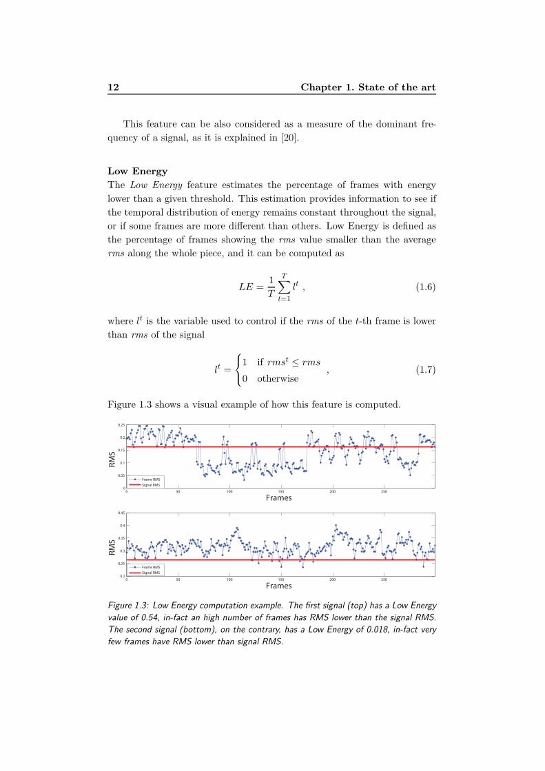
Low Energy
The Low Energy feature estimates the percentage of frames with energy
lower than a given threshold. This estimation provides information to see if
the temporal distribution of energy remains constant throughout the signal,
or if some frames are more different than others. Low Energy is defined as
the percentage of frames showing the rms value smaller than the average
rms along the whole piece, and it can be computed as
LE =1
T
T∑
t=1
lt , (1.6)
where lt is the variable used to control if the rms of the t-th frame is lower
than rms of the signal
lt =
1 if rmst ≤ rms
0 otherwise, (1.7)
Figure 1.3 shows a visual example of how this feature is computed.
0 50 100 150 200 2500
0.05
0.1
0.15
0.2
0.25
Frames
RM
S
0 50 100 150 200 2500.2
0.25
0.3
0.35
0.4
0.45
Frames
RM
S
Frame RMS
Signal RMS
Frame RMS
Signal RMS
Figure 1.3: Low Energy computation example. The first signal (top) has a Low Energy
value of 0.54, in-fact an high number of frames has RMS lower than the signal RMS.
The second signal (bottom), on the contrary, has a Low Energy of 0.018, in-fact very
few frames have RMS lower than signal RMS.

1.2. Audio Classification 13
Waveform - WF
The Waveform describes simply the shape and form of a signal. We consider
as feature the maximum and the minimum values of the WF in a frame of
the signal x. Let us consider xt as the t-th frame of the signal, so the
Waveform feature values are
W F tmax = max
(
xt)
, (1.8)
W F tmin = min
(
xt)
. (1.9)
1.2.1.2 Spectral Features
Spectral Features are Low-Level features highly related to the Timbre. This
makes them good descriptors in MIR applications. Spectral Features are
computed through the analysis of the Spectrum of the signal x, so the FFT
is needed.
Spectral Roll-Off
The Spectral Roll-Off is defined as the frequency below which 85% of the
magnitude distribution is concentrated [11]. It can be computed as
sroll = min
fKroll|
Kroll−1∑
k=0
Xk ≥ 0.85 ·K−1∑
k=0
Xk
, (1.10)
where Kroll is the spectral roll-off frequency bin and fKrollis the frequency
associated to that bin. The roll-off is another measure of spectral shape.
Figure 1.4: Spectral roll-off, graphic illustration
Spectral Brightness
The Brightness is the result of the ratio between the amount of the spectral
energy for frequencies higher than 1500Hz and the total amount of spectrum

14 Chapter 1. State of the art
energy. It can be computed as
sbright =
∑K−1k=Kc
|Xk|∑K−1
k=0 |Xk|, (1.11)
where Kc is the bin corresponding to a frequency of 1500Hz.
Figure 1.5: Spectral Brightness, graphic illustration
Spectral Flux
Spectral flux is a measure of how quickly the power spectrum of a signal is
changing [11]. It is computed as the Euclidean distance between the spectral
distributions of two adjacent frames,
sfluxt =
√
√
√
√
K−1∑
k=0
(
Xtk − Xt−1
k,
)2, (1.12)
where Xk,t is the magnitude of k-th bin of the spectrum of the t-th frame of
x and Xk,t−1 is the magnitude of k-th bin of the spectrum of the previous
frame t − 1.
Spectral Entropy
The Spectral Entropy is the Shannon’s entropy of the signal spectrum,
sentr = −
∑K−1k=0 Xk · log(Xk)
log(K). (1.13)
The presence of log(K) at the denominator makes the feature independent
from the window’s length.
Spectral Flatness
The Spectral Flatness is a measure of how tone-like a sound is. A sound is
noise-like if the spectrum is flat (i.e., it is white noise, with similar amount
of power in all spectral bands), whereas it is considered tone-like in presence

1.2. Audio Classification 15
of peaks or resonant elements. If it approaches to 0, it indicates that the
spectral power is concentrated in small number of bands. The spectral
flatness is calculated by dividing the geometric mean of the power spectrum
by the arithmetic mean of the power spectrum,
sflat =
K
√
∏K−1k=0 Xk
∑K−1
k=0Xk
K
. (1.14)
Spectral Irregularity
The Irregularity of the spectrum is a measure of the variation of successive
peaks of the spectrum. A peak is defined as a local maximum of the mag-
nitude spectrum. The Spectral Irregularity is computed as the sum of the
squared differences of adjacent peaks,
sirr =
∑M−2m=0 (pm − pm+1)2
∑M−1m=0 p2
m
, (1.15)
where pm is the m-th peak amplitude and M the number of the peaks. The
approach used for the irregularity computation is the one described in [21].
Roughness
The Roughness is an estimation of sensory dissonance [22] related to the
beating phenomenon perceived when two sinusoids are close in frequency.
According to the MIRToolBox [23] which provides an implementation of this
feature, the peaks of the spectrum are first computed and then the average
dissonance between all the possible pairs of peaks is taken, as proposed in
[24]. For all the pairs of frequency peaks (i, j), we define pi,pj as i-th and
j-th peak amplitudes, and fi, fj as frequencies corresponding to i-th and
j-th frequency peaks. The roughness ri,j is defined as
ri,j =1
2×(pipj)
0.1×
(
2pmin
pi + pj
)3.11
×(
e−3.5Z|fi−fj | − e−5.75Z|fi−fj |)
, (1.16)
wherepmin = min(pipj) ,
fmin = min(fifj) ,(1.17)
Z =0.24
0.0207 × fmin + 2π × 18.96. (1.18)
It is possible to obtain an estimation of the total roughness of the signal by
taking the average of dissonances between all the possible pairs of peaks.

16 Chapter 1. State of the art
Spectral Centroid
According to the view of the Magnitude Spectrum as a distribution function,
the first four statistical moments of the distribution are Spectral Centroid,
Spectral Spread, Spectral Skewness and Spectral Kurtosis. The Spectral Centroid
is the barycentre of the spectrum. It is calculated as the weighted average
between each frequency component, using as weight the spectral magnitude
at that frequency
sc =
∑K−1k=0 fkXk∑K−1
k=0 Xk
. (1.19)
The spectral centroid is commonly associated with the measure of the bright-
ness of a sound [25]. Many kinds of music involve percussive sounds, which
introduce high-frequency components that increase the centroid value. [26].
This is real also for a rough ”detection” of other type of noise in our sound
samples. The centroid is also called first moment (mean). In-fact some use
Spectral Centroid to refer to the median of the spectrum, although there
is a difference with the classical statistical first moment, the difference be-
ing essentially the same as the difference between the un-weighted median
and mean statistics. Since both are measures of central tendency, in some
situations they will exhibit some similarity of behaviour.
Spectral Spread
The Spectral Spread is a measure of the standard deviation of the spectrum
with respect to the spectral centroid. It can be computed as
sspread =
√
√
√
√
∑K−1k=0 Xk (fk − sc)2
∑K−1k=0 Xk
, (1.20)
where sc is the spectral centroid. It is the second central moment.
Spectral Skewness
The Spectral Skewness is the third central moment and is a measure of
the symmetry/asymmetry of the spectrum related to its mean value. It
is defined as
sskew =
∑K−1k=0 Xk (fk − sc)3
Kσ3, (1.21)
where σ is the spectral spread. If the skewness value is zero, the spectrum
is symmetrically distributed.
Spectral Kurtosis
The Spectral Kurtosis is the fourth central moment. It indicates the flatness

1.2. Audio Classification 17
of the spectrum around its mean value. It is defined as
skurt =
∑K−1k=0 Xk (fk − sc)4
Kσ4. (1.22)
If the value of the kurtosis is 3, the spectrum behaves as a Gaussian distri-
bution. If the value of kurtosis is higher, the spectral distribution takes a
slower decay and the tails are heavier.
1.2.1.3 Harmonic Features
The Harmonic Features are Mid-Level features computed from the Sinus-
oidal Harmonic Modelling of the signal. SHM represents the signal as the
linear combination of concurrent slow-varying sinusoids, grouped together
under harmonic frequency constraints.
Chroma Features and Chromagram
The Chroma Features provide a representation of audio data according to
note frequency values of the musical octave. Musical octave is an interval
whose highest note has a sound-wave frequency of vibration twice that of
its lowest note. In the chromatic scale an octave is divided by 12 equally
spaced pitches, corresponding to 12 semitones. Chroma features consist in a
redistribution of the spectrum energy along the different 12 pitches classes.
If we consider a signal x divided in several frames, the chroma features of
each frame can be computed using MIRToolBox [23]. An example of chroma
features is shown in Figure 1.6(b). Chromagram is defined as a time-ordered
set of vectors containing chroma features of all frames composing the signal.
An example of chromagram is shown in Figure 1.6(a).
Chromatic Flux
Chromatic flux is computed as the Euclidean distance between the chroma
features vectors belonging to two successive frames of the audio signal,
CF t =
√
√
√
√
12∑
i=1
(
Cti − Ct−1
i
)2, (1.23)
where Cti is the i-th value of Chroma features vector of the frame t and Ct−1
i
is the i-th value of Chroma features vector of the previous frame t − 1.
This descriptor can be helpful to detect the harmonic alteration by measur-
ing the changes from frame to frame.

18 Chapter 1. State of the art
Time (s)
ch
rom
a c
lass
(a)
0
100
200
300
400
Ma
gn
itud
e
(b)
Figure 1.6: (a) Chromagram of the entire signal that shows the time distribution of the
12 pitch classes (b) Chroma-Features of a single frame that show how the spectrum
magnitude is distributed into 12 bins, representing the 12 distinct semitones of the
musical octave
Inharmonicity
In music, inharmonicity provides a measure of the amount of partials that
are non-multiples of the fundamental frequency. More precisely, in our situ-
ation the inharmonicity takes into account the ideal and expected positions
of harmonics compared to the actual spectrum harmonics. According to the
MIRToolBox [23], a simple function estimating the inharmonicity of n-th
partial given the fundamental frequency f0 is given by
hn =|fn − nf0|
nf0, (1.24)
where fn is n-th succeeding partial, i.e., the n-th frequency of the signal
that is an integer multiple of the fundamental frequency f0.
1.2.1.4 Rhythmic Features
Rhythmic Features are Mid-Level Features that are highly related to the
rhythmic patterns played sequentially on drums. Rhythmic features are

1.2. Audio Classification 19
generally based on the onset note curve, where for onset note we intend a
peak in the time-energy diagram corresponding to the attack time of a note.
Event Density
The Event Density is the temporal average number of acoustic events, i.e.,
the average frequency of notes per second. According to the MIRToolBox
[23], it can be evaluated by counting the number of note onsets per second.
For this purpose it is needed to compute the onset detection curve, than it
is only necessary to count the onset contained by the function [23].
Pulse Clarity
Pulse Clarity estimates the rhythmic clarity, indicating the strength of the
beats. It is related to the listener’s perception of the underlying rhythmic
or metrical pulsation [27]. According to the MIRToolBox [23], it is com-
puted by taking the autocorrelation function of the onset detection curve
and normalizing it to its maximum value.
1.2.1.5 Perceptual Features
Perceptual Features are Low-Level features computed using a human per-
ceptual model. In this case, the spectrum, where the frequency bands are
positioned logarithmically, can better approximate the human auditory sys-
tem’s response.
Mel-Frequency Cepstral Coefficients - MFCC
The Mel Frequency Cepstral Coefficients are a set of features derived from
the speech recognition systems [11]. MFCCs are perceptually motivated fea-
ture and although they were developed at first for speech classification, they
have also been applied to music genre classification [11]. The MFCCs are
widely used due to their ability to represent the spectrum in a very compact
form. The computation of the Mel-Frequency Cepstral Coefficients follows
the schema illustrated in Figure 1.7 [28].
Figure 1.7: Mel-Frequency Cepstral Coefficients computational flow
The signal is divided in windowed frames and for each frame:
• The FFT X(ω) of the frame xt is computed.

20 Chapter 1. State of the art
• As shown in Figure 1.8, the amplitude spectrum X is filtered using
a set of, typically, 40 overlapping triangular band-pass filters, based
on Mel-Frequency scale. The Mel-Frequency scale is a scale of pitches
judged by listeners to be perceptually equal in distances one from
another. The following equation is used to compute the Mel for given
frequency f in Hz.
Mel = 1127.0148 log
(
1 +f
700
)
. (1.25)
1
freq
Energy in
Each Band... ...
Figure 1.8: Mel-Frequency Filter Bank
• MFCCs are obtained as the coefficients of the Discrete Cosine Trans-
form (DCT) applied to the reduced Power Spectrum. The reduced
Power Spectrum derived as the log-energy of the spectrum is meas-
ured within the pass-band of each filter of a Mel-filter bank. The m-th
MFFC coefficient is finally formalized as
MFFCm =J−1∑
j=0
{
log (Ej) cos
[
mπ
J
(
j −1
2
)]}
, (1.26)
0 ≤ m ≤ L − 1 ,
where L is the number of Mel filters and J is the number of MFCCs
derived for each frame. Ej is the spectral energy measured in the
critical band of the m-th Mel filter.
• The averaged MFCCs of all frames in a music piece are used as feature
of the whole file.
The Mel scale is used because it approximates the human auditory system’s
response more closely than the linearly-spaced frequency bands. The DCT
is used in place of the (inverse) Fourier transform because it has a strong
compactness, since the signal information are normally concentrated in a
few low-frequency components of the DCT. This is also why typically only
13 coefficients are used.

1.2. Audio Classification 21
Octave-Based Spectral Contrast - OSC
The Octave-based Spectral Contrast coefficients consider the peak and the
valley of the spectrum and the difference in each sub-band. Typically in
music strong spectral peaks roughly correspond with harmonic components,
while non-harmonic components (noise) often appear at spectral valleys [29].
The MFCCs average the spectral distribution in each sub-band and thus lose
relative spectral information. The OSC computational flow is very similar
to the MFCCs one, as shown in Figure 1.9.
Figure 1.9: Octave-Based Spectral Contrast computational flow
• The FFT is performed on the digital samples of the signal.
• The frequency domain is divided in sub-bands by several Octave-scale
filters, which are more suitable than Mel-scale for music processing. An
example of these sub-bands is given in [29], where the authors divide
the frequency domain into six Octave-scale sub-bands: 0Hz ∼ 200Hz
(we can see with refer to Table 1.1 that this first sub-band includes
two octaves), 200Hz ∼ 400Hz, 400Hz ∼ 800Hz, 800Hz ∼ 1.6kHz,
1.6kHz ∼ 3.2kHz, 3.2kHz ∼ 8kHz (another octave out of the bound
indicated in Table 1.1).
• The strength of spectral peaks and valleys can be estimated in each
sub-band. In order to ensure the steadiness of the feature, the strength
of spectral peaks and spectral valleys are estimated by the average
value in the small neighbourhood around maximum and minimum
value respectively, instead of the exact maximum and minimum value
themselves. Thus, neighbourhood factor α is introduced to describe
the small neighbourhood. α is set to 0.02 (typically is set between
0.02 and 0.2, but it does not affect the performance significantly).
The FFT of each of the j-th sub-band of the signal is returned as
a vector, than is sorted in descending order of magnitude, such that
Xj,1 > Xj,2 > ... > Xj,K , where K is the total number of FFT bins.
The strength of spectral peaks and spectral valleys are estimated as
Peakj =1
αK
αK∑
i=1
Xj,i , (1.27)

22 Chapter 1. State of the art
V alleyj =1
αK
αK∑
i=1
Xj,K−i+1 . (1.28)
• Applying the log-scaling, the Spectral Contrast of j-th sub-band is
given by
SCj = log
(
Peakj
V alleyj
)
. (1.29)
• Finally, the Karhunen-Loeve transform can be performed in order to
map the Spectral Contrast coefficients into an orthogonal space, ob-
taining the final uncorrelated OSC coefficients.
Table 1.1: Frequencies relative to the notes of the first six octaves. Each octave is
divided into 12 notes. Each note, in a certain octave, has a frequency value twice that
of the same note of the previous octave (Oct).
Note Oct=1 Oct=2 Oct=3 Oct=4 Oct=5 Oct=6
A 55.00 110.00 220.00 440.00 880.00 1,760.00
A♯/B♭ 58.27 116.54 233.08 466.16 932.33 1,864.66
B 61.74 123.47 246.94 493.88 987.77 1,975.53
C 65.41 130.81 261.63 523.25 1,046.50 2,093.01
C♯/D♭ 69.30 138.59 277.18 554.37 1,108.73 2,217.46
D 73.42 146.83 293.67 587.33 1,174.66 2,349.32
D♯/E♭ 77.78 155.56 311.13 622.25 1,244.51 2,489.02
E 82.41 164.81 329.63 659.26 1,318.51 2,637.02
F 87.31 174.61 349.23 698.46 1,396.91 2,793.83
F♯/G♭ 92.50 185.00 370.00 739.99 1,479.98 2,959.96
G 98.00 196.00 392.00 783.99 1,567.98 3,135.96
G♯/A♭ 103.83 207.65 415.31 830.61 1,661.22 3,322.42
1.2.2 Classifiers
In machine learning, classification is the problem of identifying to which
classes an observation belongs. Classes correspond to labels for different
populations (e.g., dogs and cats form separate classes). Classification has
two distinct meanings:
• on the basis of data containing observations whose class is known, the
classifier defines a rule whereby a new observation can be classified
into one of the existing classes.

1.2. Audio Classification 23
• given a set of unlabelled observations, the classifier establishes the
existence of classes or clusters in the data.
The first method is known as Supervised Learning, while the second is called
Unsupervised Learning (or Clustering) [30].
The classifier is an algorithm with features as input, and the output is usually
a label, but it can contain confidence values [31]. In supervised learning, the
set of data containing objects whose class is known, is called training set,
in which the classifier uses feature vectors to estimate a model describing a
class, provided that there are enough good samples available. Through this
model, a new object can be categorized into one of the classes analysed. In
unsupervised learning, the data are not labelled and the classifier, according
to some rules, tries to find clusters and form classes.
Since in our problem we assume that a training set is available, we have used
only supervised classifiers, and, more specifically, Gaussian Mixture Model
and Support Vector Machine [32].
1.2.2.1 Gaussian Mixture Model - GMM
Bayesian classification is based on probability theory and on the principle
of choosing the most probable option. let us assume that we need to classify
some observed data into C different classes. Each observation s is charac-
terised by a feature vector of size D. The probability that s belongs to class
wc is p(wc|s), and it is often referred to as a posteriori (or posterior) prob-
ability. The classification of the observations is done according to posterior
probabilities or decision risks calculated from the probabilities.
The posterior probabilities can be computed with the Bayes formula
p(wc|s) =p(s|wc)p(wc)
p(s), (1.30)
where p(s|wk) is the probability density function of class wc in the feature
space and p(wc) is the a priori probability, which is the probability of the
class wc without any knowledge on the feature values. If prior probabilities
are not actually known, they can be estimated by the class proportions in
the training set. The divisor
p(s) =C∑
c=1
p(s|wc)p(wc) (1.31)
is merely a scaling factor to assure that posterior probabilities are really
probabilities, i.e., their sum is one.

24 Chapter 1. State of the art
Choosing the class of with highest posterior probability produces the min-
imum error probability. The major problem in the Bayesian classifier is
estimating the class-conditional probability density function p(s|wc), that
describes the distribution of feature vectors in the feature space inside a
particular class.
GMM approach assumes that the class-conditional probability density of
the observed process can be modelled as a weighted sum of G multivariate
Gaussian probability density functions
p(s|θ) =G∑
g=1
αgbg(s) , (1.32)
where s is a vector of size D, αg is the weight corresponding to the g-th
component. bg(x) is a g-th Gaussian density function, that is defined as
bg(s) =1
2πD/2|∑
|1/2e
− 1
2(x−µg)⊤
(
∑
g
)
−1
(x−µg), (1.33)
where µg is the mean vector and∑
g is the covariance matrix of s. The
parameter list θ defines a particular Gaussian mixture probability density
function
θ ={
α1, µ1,∑
1, α2, µ2,
∑
2, ..., αG, µG,
∑
G
}
. (1.34)
Figure 1.10: An example surface of a two-dimensional Gaussian mixture PDF
In Figure 1.10 is shown an example of 2-dimensional Gaussian probab-
ility density function. In construction of a Bayesian classifier, the class-
conditional probability density functions need to be determined. The initial
model selection can be done for example by visualizing the training data,

1.2. Audio Classification 25
but the adjustment of the model parameters requires some measure of good-
ness, i.e., how well the distribution fits the observed data. Data likelihood
is a such goodness value. Let us assume that there are M independent ob-
servations s = [s1, s2, ..., sM ]⊤ drawn from a single distribution described by
a probability density function p(s|θ), a likelihood function is defined as
L(s|θ) =M∏
m=1
p(sm|θ) . (1.35)
This function supplies the likelihood of the samples with respect to the
distribution. The goal is to find θ that maximize the likelihood as
θ = arg maxθ
L(s|θ) . (1.36)
Usually this function is not maximized directly, but the logarithm
L(s|θ) = ln L(s|θ) =M∑
m=1
ln p(sm|θ) , (1.37)
called the log-likelihood function, is analytically easier to handle. Because
of the monotonicity of the logarithm function the solution to Eq. 1.36 is the
same using L(s|θ) or L(s|θ).
Depending on p(s|θ), it might be possible to find the maximum analytically
by setting the derivatives of the log-likelihood function to zero and solving
θ. It can be done for a Gaussian probability density function, which leads to
the intuitive estimates for a mean and variance, but usually the analytical
approach is intractable. In practice an iterative method such as the Expect-
ation Maximization(EM) algorithm is used. EM algorithm is employed to
estimate the GMM parameters that maximize the likelihood of a set of M
data vectors. Assuming the use of diagonal covariance matrices, the process
iteratively updates the searched parameters as expressed by the following
equations
µnewg =
∑Mm=1 p(g|sm, θ)sm∑M
m=1 p(g|sm, θ), (1.38)
∑new
g=
∑Mm=1 p(g|sm, θ)(sm − µg)⊤(sm − µg)
∑Mm=1 p(g|xm, θ)
, (1.39)
αnewg =
1
M
M∑
m=1
p(g|sm, θ). (1.40)
The element p(g|sm, θ) is computed as
p(g|sm, θ) =αgbg(sm)
∑Gg=1 cgbg(sm)
. (1.41)

26 Chapter 1. State of the art
The weight αg of a component is the portion of samples belonging to that
component. It is computed by approximating the component-conditional
probability density function with the previous parameter estimates and tak-
ing the posterior probability of each sample point belonging to the compon-
ent g. The component mean µg and the covariance matrix∑
g are estimated
in the same way. The samples are weighted with their probabilities of be-
longing to the component, and then sample mean and sample covariance
matrix are computed.
It is worth to note that so far the number of Gaussian components G is
assumed to be known, and the output is calculated depending on an initial
guess of the parameters to be maximized.
1.2.2.2 Support Vector Machine - SVM
SVM is a machine learning instrument defined as a binary classifier, meaning
that is able to infer the boundary that separates elements belonging to two
different classes. It essentially searches for an appropriate hyperplane able
to separate the classes within the feature space, i.e., able to maximize its
distance from the closest training points. Given M training vectors in the
D-dimension space, the m-th observation sn is associated to a binary class
ym ∈ {1, −1}. Assuming that data are linearly separable, it is then possible
to delineate the separation hyperplane between the two dataset groups, in
the form
β⊤s + β0 = 0 , (1.42)
where β is the vector normal to the plane, β0 is the offset, β0
||β|| is the distance
from the hyperplane to the origin.
For each sm,
• if β⊤sm + β0 ≥ 0, sm belongs to the positive class, so ym = +1 .
• if β⊤sm + β0 < 0, sm belongs to the negative class, so ym = −1 .
More precisely, the operation of the SVM algorithm is based on finding
the optimal separating hyperplane, which separates data belonging to two
classes and maximizes the distance to the closest observations from either
class. Not only does this provide a unique solution to the separating hyper-
plane problem, but, maximizing the margin between the two classes on the
training data, this leads to better classification performance on test data.
As shown in Figure 1.11, the margin is equal to 2||β|| , so SVM wants to min-
imize ||β||. Since it’s difficult to solve this optimisation problem because
||β|| involves a square root, SVM training process substitutes the equation

1.2. Audio Classification 27
margin
Figure 1.11: Support vector classifier. The decision boundary, represented by the solid
blue line, separates the observations belonging to different classes. Broken lines bound
the shaded maximal margin of width 2
||β||
without changing the solution, and solves the following quadratic program-
ming optimization through Lagrange multipliers
minimizeβ,β0
1
2||β||2 ,
subject to ym(β⊤sm + β0) ≥ 1, ∀m ∈ M .
(1.43)
An example of SVM applied to audio classification can be observed in [33].
Most of the practical problems addressed through SVM present observations
that are not separable by a hyperplane, since the edges between the classes
are not linear. In this case it is possible to turn a non-linear problem to a
linear one by using Kernel functions x → φ. The input vectors, which the
kernel function is applied on, are projected into a transformed feature space
where the data are linearly separable (Figure 1.12).
Figure 1.12: A Kernel function projects the input data into a new space where a
hyperplane can be used to separate the classes
Given a finite set of observations, it is always possible to find a dimen-
sion where all the data points are separated by a hyperplane. Hence, after
mapping the input elements to a sufficiently high-dimensional space, it is

28 Chapter 1. State of the art
possible to employ the linear SVM training approach in order to find the
optimal separating plane. The SVM is a binary classifier, but there are
several approaches to classify problems with three or more classes. The
dominant approach is to reduce the single multi-class problem into multiple
binary classification problems. Building binary classifiers which distinguish
between one of the labels and the rest (one-versus-all) or between every
pair of classes (one-versus-one). Classification of new instances for the one-
versus-all case is done by a winner-takes-all strategy, in which the classifier
with the highest output function assigns the class. For the one-versus-one
approach, classification is done by a voting strategy, in which every clas-
sifier assigns the instance to one of the two classes, then the vote for the
assigned class is increased by one vote, and finally the class with the most
votes determines the instance classification. We have used the one-versus-
one approach.
1.2.3 Feature Selection and Feature Reduction
Since not all features or attributes are relevant to a problem, we need a way
to recognize important features and assign a larger weight to information
provided by them [34]. Indeed some features prove to be highly discriminat-
ive when used to solve a specific problem, but they may interfere and reduce
accuracy for another problem. In addition, dealing with a large number of
features is costly, so using approaches to reduce features number are use-
ful also to improve performances. In this section we introduce the feature
selection and feature reduction methods used in our work.
1.2.3.1 Feature Selection Methods
A first approach used to reduce feature number is called Feature Selection,
which aims to select a subset of the existing features without applying any
transformation on the set. More specifically, given a set s = [s1, s2, ..., sD]⊤
of size D, feature selection aims to find a subset s of size D, with D < D,
that maximizes an objective function J (s) and so has the greatest ability
to discriminate between classes.
The quality of a particular feature subset is evaluated using an objective
function. There are two type of objective functions: filters and wrappers.
Filters rate feature based on general characteristics, such as interclass dis-
tance or statistic independence, without employing any mining algorithm.
Wrappers, on the other hand, evaluate subsets based on their predictive ac-
curacy when employing a particular classifier. Filters are advantageous for
their speed and for more general solutions, but they tend to create larger

1.2. Audio Classification 29
subsets. Wrappers are slower but typically do not suffer from the problem
of over-fitting, and also tend to result in subsets with higher classification
accuracy because they are trained to work with a specific classifier.
Filters select features independently of the used learning machine, using a
relevance criterion, while wrappers select feature subsets on the basis of how
well a learning machine performs. We focused on wrappers methods, and
the object function chosen is based on K Nearest Neighbour (K-NN). K-NN
is a method for classifying objects based on closest training examples in the
feature space: an object is classified by a majority vote of its neighbours,
assigning it to the most common class among its K nearest neighbours. In
our case k = 1, then the object is simply assigned to the class of its nearest
neighbour. Given a subset of features, KNN is firstly performed, then the
number of correct classified object can be computed. The subset with the
highest number of correct classifications is considered the best.
Forward Feature Selection - FWD
Forward Feature Selection is a greedy search algorithm that determines an
optimal set of features by starting from an empty set and sequentially adding
a single feature to the set if it increases the value of the chosen objective
function. The problem with this sequential approach is that it gravitates
toward local minima due to the inability to re-evaluate the usefulness of
features that were previously added. The goodness of a particular feature
subset is evaluated using an objective function, J(
sD
)
.
Starting from the empty set, forward sequentially adds a feature s+ that
maximizes J(
si + s+)
when combined with the features si that have already
been selected [35]. The steps performed by FWD are given in Algorithm 1.
Algorithm 1 FWD algorithm
1: Start with the empty set s0 = {∅}
2: Select the best feature s+ : arg maxs/∈siJ (si + s)
3: if J(
si + s+)
> J (si) then
4: Update si+1 = si + s+;
5: Got to 2
6: end if
Backward Feature Selection - BWD
Backward feature selection is similar to FWD but works in the opposite
direction. At the beginning, all the features are included into set of con-

30 Chapter 1. State of the art
sidered features. At each step, the feature s− that improves the objective
function J (s − s−) is removed from the set. As FWD, BWD is a greedy
algorithm that gravitates toward local minima due to the inability to re-
evaluate the usefulness of features that were previously discarded[35]. The
steps performed by BWD are given in Algorithm 2.
Algorithm 2 BWD algorithm
1: Start with the full set s0 = s
2: Select the worst feature s− : arg maxs∈siJ (si − s)
3: if J (si − s−) > J (si) then
4: Update si+1 = si − s−;
5: Go to 2
6: end if
Stepwise Feature Selection - SW
Stepwise selection is a mixed method between forward and backward selec-
tion. The problem with this sequential approaches is that they gravitate
toward local minima due to the inability to re-evaluate the usefulness of
features that were previously added or discarded. Stepwise selection starts
from an empty set and sequentially adds a single feature to the subset if
it increases the value of the chosen objective function. The added features
can be removed if its elimination from the subset improves the objective
function [35]. The steps performed by SW are given in Algorithm 3.
Algorithm 3 SW algorithm
1: Start with the empty set s = {∅}
2: Select the best feature s+ : arg maxs/∈siJ (si + s)
3: if J(
si + s+)
> J (si) then
4: Update si+1 = si + s+;
5: end if
6: Select the worst feature* s− : arg maxs∈siJ (si − s)
7: if J (si − s−) > J (si) then
8: Update si+1 = si − s−;
9: Go to 3
10: else
11: Go to 2
12: end if
∗ Notice that you’ll need a condition to avoid infinite loops.
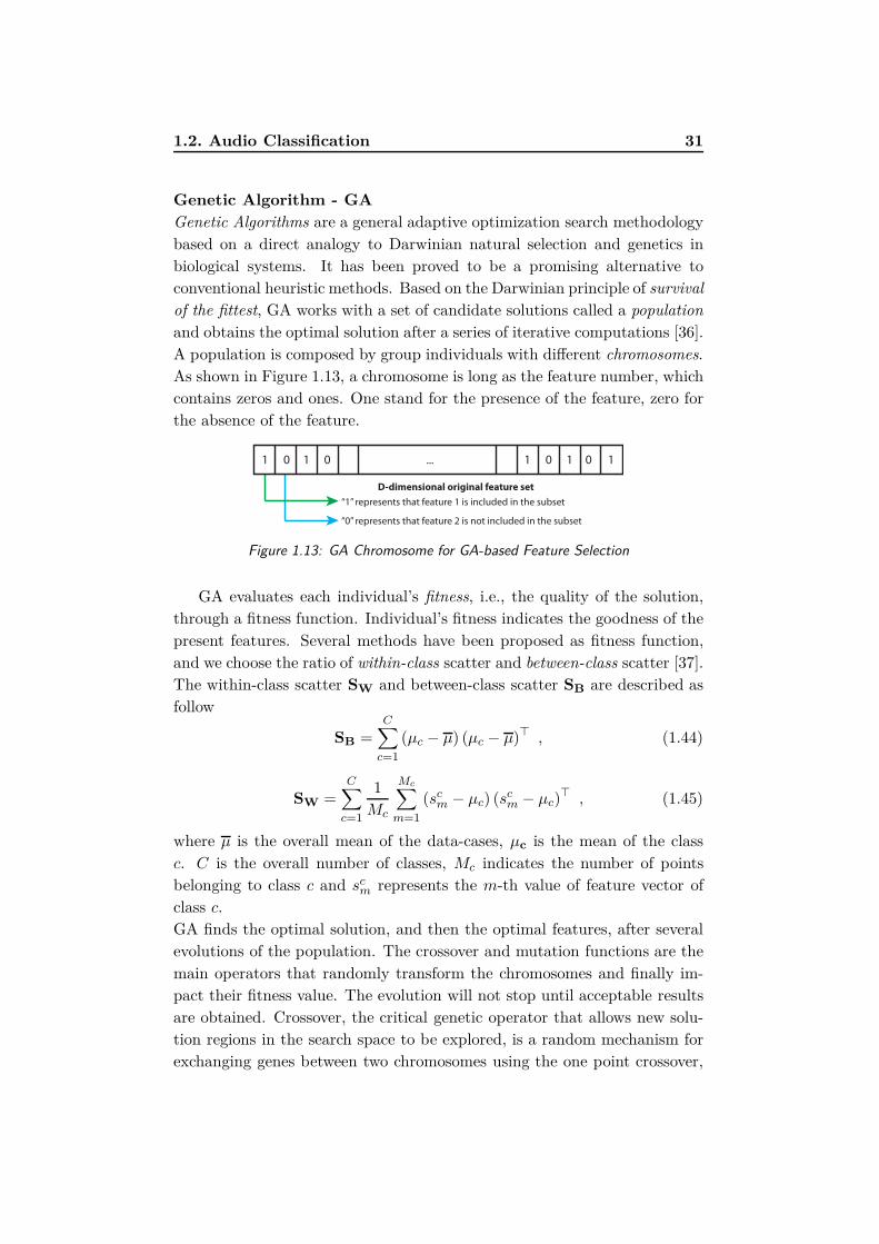
1.2. Audio Classification 31
Genetic Algorithm - GA
Genetic Algorithms are a general adaptive optimization search methodology
based on a direct analogy to Darwinian natural selection and genetics in
biological systems. It has been proved to be a promising alternative to
conventional heuristic methods. Based on the Darwinian principle of survival
of the fittest, GA works with a set of candidate solutions called a population
and obtains the optimal solution after a series of iterative computations [36].
A population is composed by group individuals with different chromosomes.
As shown in Figure 1.13, a chromosome is long as the feature number, which
contains zeros and ones. One stand for the presence of the feature, zero for
the absence of the feature.
1 1 1 1 10 0 0 0
D-dimensional original feature set
“1” represents that feature 1 is included in the subset
“0” represents that feature 2 is not included in the subset
...
Figure 1.13: GA Chromosome for GA-based Feature Selection
GA evaluates each individual’s fitness, i.e., the quality of the solution,
through a fitness function. Individual’s fitness indicates the goodness of the
present features. Several methods have been proposed as fitness function,
and we choose the ratio of within-class scatter and between-class scatter [37].
The within-class scatter SW and between-class scatter SB are described as
follow
SB =C∑
c=1
(µc − µ) (µc − µ)⊤ , (1.44)
SW =C∑
c=1
1
Mc
Mc∑
m=1
(scm − µc) (sc
m − µc)⊤ , (1.45)
where µ is the overall mean of the data-cases, µc is the mean of the class
c. C is the overall number of classes, Mc indicates the number of points
belonging to class c and scm represents the m-th value of feature vector of
class c.
GA finds the optimal solution, and then the optimal features, after several
evolutions of the population. The crossover and mutation functions are the
main operators that randomly transform the chromosomes and finally im-
pact their fitness value. The evolution will not stop until acceptable results
are obtained. Crossover, the critical genetic operator that allows new solu-
tion regions in the search space to be explored, is a random mechanism for
exchanging genes between two chromosomes using the one point crossover,

32 Chapter 1. State of the art
two point crossover, or homologue crossover. In mutation the genes may
occasionally be altered, for example, changing the gene value from 0 to 1
or vice versa in a binary code chromosome. The fitter chromosomes have
higher probability to be kept in the next generation or be selected into the
recombination pool using the tournament selection methods. If the fittest
individual or chromosome in a population cannot meet the requirement, suc-
cessive populations will be reproduced to provide more alternate solutions.
The principal steps of GA algorithm are the following:
1. Create an initial population of certain size.
2. Calculate the fitness value of each individual in the initial population
and rank them according to their fitness.
3. Select a certain number of individuals with high fitness value as elitism
of the population and retain them in the next generation.
4. Check whether the termination conditions are satisfied. If so, the evol-
ution stops and the optimal result represented by the best individual is
returned. Otherwise, the evolution continues and the next generation
is produced. The termination conditions can be either a predefined
fitness threshold or number of generation evolved.
5. If the population continues to evolve, the next generation is produced
following the procedure below. First, a certain number of individuals
are selected randomly to compete the mating right. Two individuals
of the highest fitness values are selected as a pair of parents. Crossover
is operated on their chromosomes to produce two children individuals.
Location of the crossover point on the chromosomes is also randomly
determined; second, a floating-point number in the range of 0.0 to 1.0
is generated randomly. If it is less than the predefined mutation pos-
sibility, mutation is operated for the two children individuals; Repeat
these steps to produce all the children individuals (except the elitism
individuals) in the new generation.
6. Go to step 2.
Feature Selection with RELIEF algorithm - RE
This method addresses the feature selection problem by proposing a two-
step algorithm [38]: the first step uses a variation of the well-known Relief
algorithm to remove irrelevance; the second step clusters features using K-
means to remove redundancy. Relief is a feature weight based algorithm

1.2. Audio Classification 33
inspired by instance-based learning. Given training data, and a threshold
of relevancy r, Relief detects those features which are statistically relevant
to the target concept. Taken at random an instance s, the nearest element,
according to the Euclidean distance, of the same class and the nearest one
of the another class are picked. If the features values of instances that
belong to different classes are far, their weights are increased, otherwise
if the values of instances of the same class are different, their weights are
decreased. Differences of feature values between two instances s1 and s2 are
defined by the following function
diff (s1,d, s2,d) =s1,d − s2,d
s1,d + s2,d, (1.46)
where s1,d and s2,d are the values of d-th feature of s1 e s2.
We show in Algorithm 4, the pseudo-code of the RELIEF algorithm [39],
where D is the total amount of features and only two classes are considered.
Algorithm 4 RE algorithm
1: Separate S into
S1 = {instances of first class}
S2 = {instances of second class}
2: W = 0D
3: for m = 1 to M do
4: Pick at random an instance s ∈ (S1)
5: Pick the instance closest to s, z1 ∈ S1
6: Pick the instance closest to s, z2 ∈ S2
7: if s ∈ (S1) then
8: Near-hit = z1; Near-miss= z2
9: else
10: Near-hit = z2; Near-miss= z1
11: update-weight (W, s, Near-hit, Near-miss)
12: end if
13: end for
14: for d = 1 to D do
15: if Wd ≥ r then
16: fd is a relevant feature
17: else
18: fd is an irrelevant feature
19: end if
20: end for

34 Chapter 1. State of the art
where update-weight is defined in Algorithm 5.
Algorithm 5 Update-Weight
1: for d = 1 to D do
2: Wd = Wd − diff(sd, Near-hitd)2 + diff(sd, Near-missd)2
3: end for
If Wd ≤ 0, then the d-th feature is irrelevant, otherwise it is significant.
The second step is a redundancy filter that uses the k-means algorithm to
cluster features according to how well they correlate to each other. When
feature clusters are discovered, only the feature with the highest Relief score
is kept; the other features in the cluster are removed from the feature set.
This is an unusual application of K-means clustering, in which features are
clustered (instead of samples). There is a partition of D features into k
clusters in which each feature belongs to the cluster with the nearest mean.
1.2.3.2 Feature Reduction Methods
A second approach used to reduce feature number is called Feature Reduc-
tion. Feature reduction aims to create a subset of new features by combin-
ations of the existing features. Let us consider a vector s = (s1, s2, ..., xD)⊤
∈ RD containing all the D features. Feature Reduction finds a mapping
s = [s1, s2, ..., sD]⊤ with D < D such that the transformed feature vector
s ∈ RD preserves (most of) the information or structure in RD. In general,
the optimal mapping will be a non-linear function, but since there is no
systematic way to generate non-linear transforms, the selection of a partic-
ular subset of transforms is problem dependent. For this reason, feature
extraction is commonly limited to linear transforms:
s1
s2...
sD
=
α11 α12 · · · α1D
α21 α22 · · · α2D...
.... . .
...
αD1 αD2 · · · αDD
s1
s2...
sD
(1.47)
where αd,d is the weight associated to sd.
Principal Component Analysis - PCA
Principal component analysis is an unsupervised method that involves a
mathematical procedure transforming a number of (possibly) correlated vari-
ables into a (smaller) number of uncorrelated variables called principal com-
ponents, which present the relevant characteristic of being uncorrelated with

1.2. Audio Classification 35
respect to each other. In particular, the largest variance of any projection of
the data lies on the first variable, the second largest variance on the second
variable, and so on (Figure 1.14).
Usually, PCA is used to discover or reduce the dimensionality of the data
set, or to identify new meaningful underlying variables. Principal compon-
ents are found by extracting the eigenvectors and eigenvalues of the cov-
ariance matrix of the data. These components are the eigenvectors, which
describe an orthonormal basis that is effectively a rotation of the original
Cartesian basis [40].
In order to reduce the dimensionality of the space, principal compon-
ents associated to small eigenvalues can be discarded. Indeed they bring
a smaller amount of information than principal components associated to
high eigenvalues.
Figure 1.14: PCA transformation in 2 dimensions. The variance of the data in the
Cartesian space x, y is best captured by the basis vectors v1 and v2 in a rotated space.
The main steps of the PCA algorithm are shown in Algorithm 6.
Algorithm 6 PCA algorithm
1: Computing covariance matrix
2: Computing eigenvalues and eigenvectors of the covariance matrix
3: Ordering the eigenvalues σ1 > σ2 > ... > σn
4: If exists σk ≪ σ1 then we can eliminate the eigenvalue and relative
eigenvectors from k to n
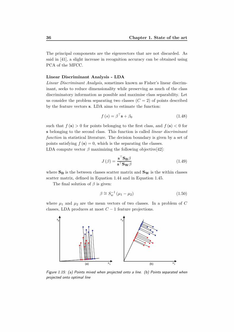
36 Chapter 1. State of the art
The principal components are the eigenvectors that are not discarded. As
said in [41], a slight increase in recognition accuracy can be obtained using
PCA of the MFCC.
Linear Discriminant Analysis - LDA
Linear Discriminant Analysis, sometimes known as Fisher’s linear discrim-
inant, seeks to reduce dimensionality while preserving as much of the class
discriminatory information as possible and maximise class separability. Let
us consider the problem separating two classes (C = 2) of points described
by the feature vectors s. LDA aims to estimate the function:
f (s) = β⊤s + β0 (1.48)
such that f (s) > 0 for points belonging to the first class, and f (s) < 0 for
s belonging to the second class. This function is called linear discriminant
function in statistical literature. The decision boundary is given by a set of
points satisfying f (s) = 0, which is the separating the classes.
LDA compute vector β maximizing the following objective[42]:
J (β) =s⊤SBβ
s⊤SWβ(1.49)
where SB is the between classes scatter matrix and SW is the within classes
scatter matrix, defined in Equation 1.44 and in Equation 1.45.
The final solution of β is given:
β ∼= S−1w (µ1 − µ2) (1.50)
where µ1 and µ2 are the mean vectors of two classes. In a problem of C
classes, LDA produces at most C − 1 feature projections.
(b)(a)
Figure 1.15: (a) Points mixed when projected onto a line. (b) Points separated when
projected onto optimal line

1.2. Audio Classification 37
Chapter Conclusions
In this Chapter we have presented a brief overview of forensic works related
to ours, and the main tools used to solve our classification problem. In the
next Chapter we will show how to use these tools for our purpose.

This page is intentionally left blank.
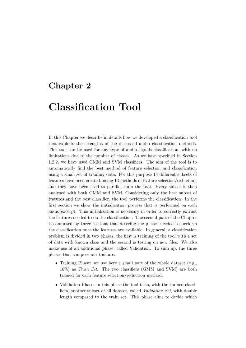
Chapter 2
Classification Tool
In this Chapter we describe in details how we developed a classification tool
that exploits the strengths of the discussed audio classification methods.
This tool can be used for any type of audio signals classification, with no
limitations due to the number of classes. As we have specified in Section
1.2.2, we have used GMM and SVM classifiers. The aim of the tool is to
automatically find the best method of feature selection and classification
using a small set of training data. For this purpose 13 different subsets of
features have been created, using 13 methods of feature selection/reduction,
and they have been used to parallel train the tool. Every subset is then
analysed with both GMM and SVM. Considering only the best subset of
features and the best classifier, the tool performs the classification. In the
first section we show the initialization process that is performed on each
audio excerpt. This initialization is necessary in order to correctly extract
the features needed to do the classification. The second part of the Chapter
is composed by three sections that describe the phases needed to perform
the classification once the features are available. In general, a classification
problem is divided in two phases, the first is training of the tool with a set
of data with known class and the second is testing on new files. We also
make use of an additional phase, called Validation. To sum up, the three
phases that compose our tool are:
• Training Phase: we use here a small part of the whole dataset (e.g.,
10%) as Train Set. The two classifiers (GMM and SVM) are both
trained for each feature selection/reduction method.
• Validation Phase: in this phase the tool tests, with the trained classi-
fiers, another subset of all dataset, called Validation Set, with double
length compared to the train set. This phase aims to decide which

40 Chapter 2. Classification Tool
feature selection/reduction method gives the most relevant features
and which is the best type of classifier (relative to the best feature
selection method).
• Test Phase: now the tool is ready to test any file with the methods
selected in the validation phase.
We describe out tool starting from the classical composition of a classifica-
tion tool, then we introduce the details on the Validation Phase.
2.1 Files Initialization
The classification occurs when all the necessary features have been extrac-
ted from the audio excerpts. In order to correctly extract all features, an
initialization phase is required.
2.1.1 Normalization
The first step is to reduce audio files in stereo (2 channels, so 2 parallel set
of samples) to mono signal. This is simply done averaging the two channels
sample by sample: in this way also signal with one channel can be processed.
The second, a very important step, is the normalization, that is required
since it is possible to find signals with very low or very high sample amplitude
(i.e., see Figure 2.1 and 2.2), when this happens, features extracted from such
an audio excerpt may be distorted and thus not valid.
0 0.5 1 1.5 2 2.5
x 106
−1
−0.5
0
0.5
1
Time (samples)
Am
pli
tud
e
0 0.5 1 1.5 2 2.5
x 106
−1
−0.5
0
0.5
1
Time (samples)
Am
pli
tud
e
Figure 2.1: Two audio signals with very different amplitude

2.1. Files Initialization 41
0 0.5 1 1.5 2 2.5
x 106
−1
−0.5
0
0.5
1
Time (samples)
Am
pli
tud
e
0 0.5 1 1.5 2 2.5
x 106
−1
−0.5
0
0.5
1
Time (samples)
Am
pli
tud
e
Figure 2.2: The same audio signal as figure 2.1 after the normalization have been
performed on each file.
Audio normalization is the application of a constant amount of gain to an
audio signal to bring the average or peak amplitude to a target level (the
norm). Because the same amount of gain is applied across the given range,
the signal-to-noise ratio and relative dynamics are generally unchanged. We
have forced the signal to have unitary peak amplitude (maximum peak with
amplitude 1 in absolute value). The gain applied to each signal considered
is variable and it depends on the signal itself. The equation of the normal-
ization is:
x =xo
max |xo|, (2.1)
where xo is the original signal before normalization.
2.1.2 Frame Division
Once the normalization has been applied, the signal is subdivided in frames.
This division has been performed because some features need to be extracted
for frames of signal. Anyway, there are some features extracted for the
global signal and others that are extracted in both cases. The frames can
have constant or variable length. We have divided each excerpt in a variable
number of frames where the length of each frame depends on the energy that
it contains. This decision has been made to avoid the presence of frames
containing silence, or too much noise. The energy contained in each frame is
constant and the amount of audio information carried is somehow equalized.
The effect is that part of signal with low amplitude causes the creation of
longer frames, while short frames are created in case of part rich in energy.
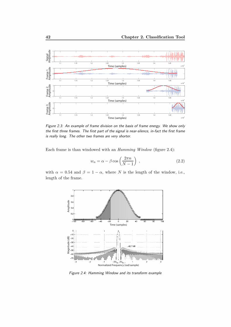
42 Chapter 2. Classification Tool
1.1 1.15 1.2 1.25 1.3 1.35 1.4 1.45
x 106
−1
0
1
Time (samples)
Sig
na
lA
mp
litu
de
1.1 1.15 1.2 1.25 1.3 1.35 1.4 1.45
x 106
−1
0
1
Time (samples)
Fra
me
1A
mp
litu
de
1.1 1.15 1.2 1.25 1.3 1.35 1.4 1.45
x 106
−1
0
1
Time (samples)
Fra
me
2A
mp
litu
de
1.1 1.15 1.2 1.25 1.3 1.35 1.4 1.45
x 106
−1
0
1
Time (samples)
Fra
me
3A
mp
litu
de
Figure 2.3: An example of frame division on the basis of frame energy. We show only
the first three frames. The first part of the signal is near-silence, in-fact the first frame
is really long. The other two frames are very shorter.
Each frame is than windowed with an Hamming Window (figure 2.4):
wn = α − β cos
(
2πn
N − 1
)
, (2.2)
with α = 0.54 and β = 1 − α, where N is the length of the window, i.e.,
length of the frame.
Time (samples)
Normalized Frequency (rad/sample)
Ma
gn
itu
de
(d
B)
Am
plit
ud
e
Figure 2.4: Hamming Window and its transform example

2.1. Files Initialization 43
2.1.3 Feature Extraction
After the first two phases, the signal is ready and the features can be ex-
tracted. Features are extracted both from each frame and from the entire
signal. What we obtain is a set of 14 features for each frame (Frame Fea-
tures) and 20 for the entire signal (Global Features). We have then grouped
the features in different sets, as it is shown in Table 2.1. This subdivision is
used to train the tool in two different cases, with all the features in a single
macro-set and with the features divided in groups. The creation of different
groups of features is inspired by [43] and the groups are formed following
principally the division explained in Section 1.2.1. This decision has been
made mainly to isolate some features as the MFCC, which are statistically
very significant and can mask the information derived from other features.
Table 2.1: Subdivision of features in groups. Frame and Global indicate if a feature is
extracted frame by frame, from the global file or in both cases. Numbers in parenthesis
indicate features composed by multiple values, e.g., the MFCCs have 13 coefficients.
Features Group Feature Name Frame Global
Basic
RMS X X
ZCR X X
WF (2) X
Low Energy X
Spectral
S. Roll-Off X X
S. Brightness X X
S. Flux X X
S. Entropy X X
S. Flatness X X
S. Irregularity X X
S. Roughness (2) X
Centroidal
S. Centroid X X
S. Spread X X
S. Skewness X X
S. Kurtosis X X
HarmonicS. Inharmonicity X
Chromatic Flux (2) X
RhythmicEvent Density X
Pulse Clarity X
MFCC MFCC (13) X X
OSC OSC (8) X

44 Chapter 2. Classification Tool
In the following sections we explain more in detail how the feature subdivi-
sion is used in the classification. The tool we have built potentially support
multi-class, but for our purpose we have used only two classes. So, also
to simplify the exposition, from now on we consider only the classification
between two classes (A and B).
2.2 Training Phase
When all the features are extracted, the tool can switch to the classification
phase, which begins with the Training Phase. This phase aims to train the
classifiers that the tool will use in the test phase. Starting from all the
dataset, the tool randomly choose a small percentage of files with known
class membership. It is very important that in the creation of the Training
Set the number of files belonging to each classes is the same; otherwise the
risk is to train the tool with a significant amount of bias. The parameters,
needed from the classifiers in the Test Phase to recognize the membership
classes, are then computed. Motivated by [43], we trained the classifiers with
both features taken all together, and features divided into groups (defined in
Table 2.1). We show now a flow chart (Figure 2.5) of the steps of Training
Phase for the case of features taken as macro-set. In case of features grouped
in different sets the flow is the same, but each block is further subdivided.
Figure 2.5: Training Phase Flow Chart

2.2. Training Phase 45
To better understand the following description of the Training Phase, make
reference to Figure 2.5. Once the training set is chosen, the tool can train the
classifiers (GMM and SVM). The values of the features extracted for each
frame of files in training set are examined by a method of feature selection,
which selects only discriminant features. Each method has different way to
consider which features are significant and which can be discarded because
of their correlation to other features. When the features are considered as
a macro-group, feature selection is applied to all the set together, while in
case of features divided in groups, the same feature selection is applied inside
each group.
2.2.1 Feature Selection and Reduction Methods
Since we extract a lot of features, some of these can be useless for a particular
classification. So we want to find an optimal subset of features that contains
the most significant ones to be used during the test. For this purpose, we
use different types of feature selection and reduction methods.
In particular we made use of the following methods that have been presented
in Section 1.2.3:
• Forward Feature Selection (FWD)
• Backward Feature Selection (BWD)
• Stepwise Feature Selection (SW)
• Genetic Algorithm Selection (GA)
• Relieff Algorithm Selection (RE)
• Principal Component Analysis (PCA)
• Linear Discriminant Analysis (LDA)
and we combined them in 13 different methods. Each method considers as
significant a different subset of feature. Note that most of the computational
time is due to the extraction of the features. So testing a high number of
feature selection/reduction methods does not contribute to highly increment
the tool computational time and complexity.
NO feature selection method applied
In this case, we make use of all the features, without using any feature
selection method. It is expected that analysing all the features, the classific-
ation accuracy is worse than that obtained after selecting a subset of these
features.

46 Chapter 2. Classification Tool
FWD selection
A subset of features is obtained by FWD selection algorithm. Starting from
an empty set, a single feature is sequentially added in the set if the object
function increases, until the optimal subset is found. The object function
chosen is based on 1-NN.
BWD selection
A subset of features is obtained by BWD selection algorithm. Starting
from the full set, a single feature is removed if its elimination increases or
minimally worsens the objective function, in order to obtain the best subset
of features. In this case, the object function used is based on 1-NN.
SW selection
A subset of features is obtained by SW selection algorithm. Starting from an
empty set, a single feature is sequentially added to the subset if it increases
the value of the chosen objective function. The added features can be re-
moved subsequently if its elimination from the subset improves the objective
function. The object function used is based on 1-NN.
GA selection
A subset of features is obtained by GA selection algorithm. It is charac-
terized by a heuristic search that mimics the process of natural evolution,
obtaining the optimal subset using techniques such as mutation, selection,
and crossover.
RE + FWD selection
A subset of features is obtained by a combination between RE and FWD
selection algorithms. RE tries to remove irrelevance and redundancy in the
set, and FWD selects the features that considers significant. This method
is efficient for large data sets with lots of irrelevant and redundant features.
RE + BWD selection
A subset of features is obtained by a combination between RE and BWD
selection algorithms. RE tries to remove irrelevance and redundancy in the
set, and BWD selects the features that considers significant. This method
is efficient for large data sets with lots of irrelevant and redundant features.
RE + SW selection
A subset of features is obtained by a combination between RE and SW
selection algorithms. RE tries to remove irrelevance and redundancy in the

2.2. Training Phase 47
set, and SW selects the features that considers significant. This method is
efficient for large data sets with lots of irrelevant and redundant features.
PCA
An orthogonal transformation is used to convert a set of possibly correlated
features into a set of values of linearly uncorrelated features called principal
components. The number of principal components is less than or equal to
the number of original features.
PCA + FWD selection
A subset of features is obtained by a combination between PCA and FWD
selection algorithms. First of all, PCA transforms the original features in
uncorrelated features. Then FWD selects the features that considers signi-
ficant.
PCA + BWD selection
A subset of features is obtained by a combination between PCA and BWD
algorithms. First of all PCA transforms the original features in uncorrelated
features. Then BWD selects the features that considers significant.
PCA + SW selection
A subset of features is obtained by a combination between PCA and SW
algorithms. First of all PCA transforms the original features in uncorrelated
features. Then SW selects the features that considers significant.
LDA
A linear combination of features is used in order to preserve as much of
the class discriminatory information as possible, projecting objects from the
same class very close to each other and, at the same time, objects from
different classes as farther apart as possible.
PCA Group
This method can be used only if the features extracted are divided in groups.
The basic idea is to find the feature group that has the best discriminative
power. Analysing the classification results obtained using all the features
without any selection method, the features group with the best accuracy
can be found. The best group is momentarily put aside and the other fea-
tures groups are combined and transformed by PCA. Then the final optimal
subset is composed by the principal components computed in PCA with the
addition of the most discriminant feature group previously found [44].

48 Chapter 2. Classification Tool
2.2.2 Training Steps
Once the feature selection/reduction is applied, we obtain a subset of all
features. The tool trains the classifiers relatively to the features subset.
The classifiers are separately trained both for frames and global features,
and also the global features are previously selected with the same method
used for frames feature selection. The same procedure is then applied to the
SVM classifier, also in this case separately for frames and global features.
We obtain four classifiers, two for the GMM case and two for the SVM one,
trained for each method of feature selection/reduction. We must specify
that in case of groups of feature, we have trained a GMM and a SVM for
each group and for both Frame Features and Global Features.
In the next section we explain how the classification is done.
2.3 Test Phase
Once the train is performed, the tool is ready to test a new file and to classify
it. We specify now how the tool merges the results derived from the decision
taken over different frames. As we said, the tool considers each frame as
different signal with no correlation between frames derived from same files,
then, once a decision has been made for the frames, the tool merge the
results. Let us now analyse more in depth how the finale decision is taken.
The test is performed using both the global and frame-wise features. In
particular, if we consider a single song, we split the classification phase in
three steps (as shown in Figure 2.6):
Figure 2.6: Decision merging flow

2.3. Test Phase 49
• first we independently classify every frame (using the features extrac-
ted frame-wise);
• then the global features are used to classify the whole song;
• finally results from the previous steps are merged to take the final
decision.
In the case of features divided in groups, the followed schema is the same,
but an additional step is involved: for each frame we compute the mean of
the decisions taken singly for each feature group 2.7(a). The same we can
say for the features obtained for the global signal 2.7(b). The two blocks
created (Frame t Decision and Global File Decision) are the same blocks
that appear in 2.6.
(a) Decision combination for groups of features. Each Frame Decision is the decision taken
for a single frame.
(b) Decision combination for groups of features. Global Decision
Figure 2.7: Combination of results in case of training and validation with feature groups.
Let us now consider a single feature selection method. Assuming that a
file is subdivided in T frames, we can explain in details how the final clas-
sification is computed. Note that in the case of groups of features, the first
step is the one shown in Figure 2.7, then the steps are exactly the following.
The GMM/SVM trained with the features selected gives to each frame a
probability of belonging to a class. Note that GMM provides directly prob-
abilities, but SVM simply returns the class membership of an observation.

50 Chapter 2. Classification Tool
From SVM results we can obtain the distance of the observation from sep-
arating hyperplane. We have assigned a percentage of membership of an
observation to a class according to its distance from the hyperplane. Given,
e.g., a set of MA observations belonging to class A, we give to the observation
with maximum distance from the hyperplane a probability of membership
of 100%. The probabilities of other observations are directly proportional
to their distance from the hyperplane. Computed the percentages of each
frame, we take the average of the frame probabilities. Frame probabilities
are stored then in a matrix.
F =
f1,A f1,B
f2,A f2,B...
...
fT,A fT,B
, (2.3)
where ft,A is the probability of the t-th frame to belong to class A, and ft,B
is the probability of the t-th frame to belong to class B.
The Frame Mean Decision F is the decision derived by the combination of T
frames and it is defined as the average of the probabilities of the frame-wise
decision,
F =[
fA fB
]
=1
TF⊤1T , (2.4)
where 1T is a column vector of ones of length T . The GMM trained for the
global features takes separately his decision
g =[
gA gB
]
, (2.5)
where gA is the probability that a file belongs to class A considering only the
global feature. Then, averaging the results, the final membership is given.
The probability for an audio object to belong to class A or B is given by
p =[
pA pB
]
, (2.6)
where
pA =gA + fA
2,
pB =gB + fB
2.
(2.7)
The object is then assigned to the class with the higher probability.
These steps are repeated for all the feature selection methods and both in
case of GMM and SVM classifier. When the tests with all the combina-
tion are computed, we can also compare the results of each combination.
However, we have introduced an intermediate pre-test phase that compares
the method combinations before the Test Phase, in order to choose the best
classification method beforehand (see Figure 2.8).

2.4. Pre-Test: Validation Phase 51
Figure 2.8: Tool Work Flow: the Training Phase is repeated for each Feature Se-
lection/Reduction, each combination is validated and the Test is computed using the
information derived from the Validation Phase.
2.4 Pre-Test: Validation Phase
Since we trained many classifiers, we want to be able to choose the one
that best fits our needs. In particular, if we want to classify some audio
excerpts, we need to know which classifier to use. The Validation Phase

52 Chapter 2. Classification Tool
is then introduced to solve this problem. This phase is inserted between
Training and Test phase and can also be considered as a Pre-Test. Indeed,
a Validation Set of audio excerpts is tested using all the classifiers trained
during the training phase. The Validation Set is composed by twice the
number of tracks than the Training Set, and it contains files whose class is
known. This way we evaluate the configuration of feature selection method
and classifier that maximize the accuracy in our classification problem. A
file is considered both as divided in frame and global, as in the Train Phase.
The frames are tested separately and singly, then the average of the results
is taken and further averaged with the result obtained with the classification
of the global features.
The entire Validation Set is tested, obtaining a final decision for each
file both for GMM and SVM. Now, since in the Validation Set we have files
with known class, we can evaluate some statistical parameter to determine
which configuration is the best one for the classification problem considered.
To do that, we use the combination of three parameters. The first para-
meter is the accuracy, that is defined as
accuracy =TA + TB
TA + TB + FA + FB, (2.8)
where TA and TB (True member of a class) are the number of files re-
spectively of the first and second classes correctly classified, while FA (False
member of a class) are the number files of the first class classified as files of
the second class and FB is the vice-versa. Since it may happen that the same
accuracy level is achieved by different methods, we have introduced also the
class recall and a sort of precision indicator. The recall is the fraction of
elements of a class that are correctly classified, that is, for class A and class
B
recallA =TA
TA + FB,
recallB =TB
TB + FA.
(2.9)
When two methods have the same accuracy, we consider as best method the
one with lower differences between recalls. This means that the percentage
between the recall of the classes is more similar. We have chosen this solution
because is preferable to have recall percentages of 78% and 82% respectively
for two classes than have percentages of 70% and 90%. Indeed, the second
case may indicate that the tool is biased towards one of the classes.
Another parameter considered is what we have called strictness, that
is the percentage with which the classifier make a good decision. We said

2.4. Pre-Test: Validation Phase 53
that for each file the tool return two percentages. If a result is pA = 75%
and pB = 25% it means that the considered file belongs at 75% to class A.
The strictness is the average of all the percentage of the files that have been
correctly classified in the validation phase.
Once the tool has detected which combination between macro-set of
features or groups of features, feature selection (reduction) and classifiers
(GMM-SVM) is the best, the Test Phase begins.
The procedure is the same as the one presented in before, but a file is now
tested only with the best combination (see Figure 2.9).
Figure 2.9: Test Phase Flow Chart: the classification is determined by the best com-
bination of feature selection and classifier choose in the Validation Phase
The test phase can be used both to analyse a new file and to validate the
pre-test. In this second case we obviously need a set of files with a known
class membership, then the same parameters used to evaluate the methods
combinations in the Validation Phase can be computed.
Chapter Conclusions
We have so designed a tool with the purpose of classifying audio signals,
without any restriction on the type of classification that can be carried out.
The tool is general because the features extracted are several and standard.
In the next section we present the changes and the addition made to the
tool in order to improve the results for the special case of Bootleg Detection.

This page is intentionally left blank.

Chapter 3
Bootleg Detection
Application
In the last few years the quality of audio bootleg available on-line is in-
creased, thanks to the development of new technologies. Indeed, nowadays,
every smart-phone and camera come equipped with an integrated micro-
phone. A typical example of bootleg availability is given by the huge amount
of user-generated music-related videos on websites such as YouTube. In this
case, even if the video quality may be poor, audio quality is often pretty
good. It is worth to note that the definition of bootleg is pretty wide. In-
deed both audio files directly recorded at a concert with a hand-held camera,
and songs professionally mixed and published without authorization may be
considered bootleg. For this reason, in order to cope with this situation,
a more in depth analysis of what can be considered bootleg is in order.
We define audio bootlegs as all those audio files that are recorded directly,
e.g., at a concert, from public with some device, like a smart-phone, video-
camera or microphone. In the case that a song is recorded and mixed with
professional instruments and then published without the authorization of
the owners of the song, we can’t be able to recognize the difference.
We can see in Figure 3.1 and Figure 3.2 the flow charts representing the
two main possible chains of operations that might lead to bootleg genera-
tion. Figure 3.1 shows the case of studio recording. In this situation we
can consider as bootleg audio files taken directly in the recording room with
a microphone or the audio signal after the first phase of mixing. In the
second situation we have an output from the mixer, but it is not already
been processed to obtain a perfectly clean audio without noises and with
some post-processing add as, e.g., particular reverberation or other effect

56 Chapter 3. Bootleg Detection Application
that can be directly recorded before being processed, e.g., to remove noise
or apply audio effects such as reverberation.
Figure 3.1: Studio Recording Flow Chart
Figure 3.2 shows the live performance case. In this situation we can consider
as bootleg a signal recorded directly with some device such as smart-phone,
video-camera, voice-recorder, etc. However, we can also consider the files
directly taken from the mixer and not post-processed. In this second case is
much more difficult to find differences between such a bootleg and an official
released live performance. However, this kind of bootleg is pretty rare.
Figure 3.2: Live Performance Flow Chart
In this Chapter we explain in details how to adapt the classification tool
described in Chapter 2 to work with the particular case of Audio Bootleg
Detection. As we said, the classification tool that we implemented is modular
and highly configurable. E.g., it is possible to add new features or new
methods of feature selection and reduction.
In order to solve the Audio Bootleg Detection problem, we propose three
specific improvements:
• a pre-processing phase;
• new Bootleg-related features;
• a new feature selection method.

3.1. Pre-Processing: Filter Bank 57
In the following we explain which kind of pre-processing we propose,
what are the new features introduced and how the new method of feature
selection works.
3.1 Pre-Processing: Filter Bank
This Pre-Processing phase is meant to be applied between the normaliza-
tion of the signal and its subdivision in frames (see Section 2.1). The mono
signal is processed by a Filter-Bank that creates other 10 versions. We ad-
ded this filter-bank because the Bootlegs generally have background noises
higher that Official files. We expect a better classification accuracy consid-
ering features derived from critical bands, where noises are more relevant.
So, the goal of the pre-processing phase is to extract features not only from
the original audio signal, but also for its filtered versions. As filter-bank,
we have used 10 different Finite Impulse Response (FIR) filters with Kaiser
window [45], chosen experimentally as good compromise between computa-
tional speed and precision in the band filtering.
z–1
z–1
z–1
Figure 3.3: A discrete-time FIR filter of order N.
The filter is designed with the Window Method, that is the creation of an
ideal IIR (Infinite Impulse Response) and then the application of the window
function. The result is the convolution between the frequency response
of the IIR filter and the frequency response of the window function. The
parameters of the Kaiser Window are setted to obtain a side-lobe attenuation
of 80 dB.
We have subdivided the signal following the octave scale:
• Band 1: Low-Pass filter with stop frequency at 60 Hz
• Band 2: Band-Pass filter between 60 Hz and 230 Hz
• Band 3: Band-Pass filter between 230 Hz and 500 Hz
• Band 4: Band-Pass filter between 500 Hz and 1 kHz
• Band 5: Band-Pass filter between 1 kHz and 2 kHz
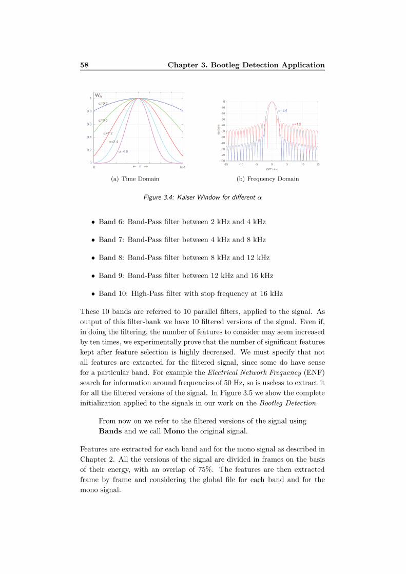
58 Chapter 3. Bootleg Detection Application
(a) Time Domain (b) Frequency Domain
Figure 3.4: Kaiser Window for different α
• Band 6: Band-Pass filter between 2 kHz and 4 kHz
• Band 7: Band-Pass filter between 4 kHz and 8 kHz
• Band 8: Band-Pass filter between 8 kHz and 12 kHz
• Band 9: Band-Pass filter between 12 kHz and 16 kHz
• Band 10: High-Pass filter with stop frequency at 16 kHz
These 10 bands are referred to 10 parallel filters, applied to the signal. As
output of this filter-bank we have 10 filtered versions of the signal. Even if,
in doing the filtering, the number of features to consider may seem increased
by ten times, we experimentally prove that the number of significant features
kept after feature selection is highly decreased. We must specify that not
all features are extracted for the filtered signal, since some do have sense
for a particular band. For example the Electrical Network Frequency (ENF)
search for information around frequencies of 50 Hz, so is useless to extract it
for all the filtered versions of the signal. In Figure 3.5 we show the complete
initialization applied to the signals in our work on the Bootleg Detection.
From now on we refer to the filtered versions of the signal using
Bands and we call Mono the original signal.
Features are extracted for each band and for the mono signal as described in
Chapter 2. All the versions of the signal are divided in frames on the basis
of their energy, with an overlap of 75%. The features are then extracted
frame by frame and considering the global file for each band and for the
mono signal.

3.2. Bootleg Detection Specific Features 59
Figure 3.5: File Initialization Flow Chart for Bootleg Detection
3.2 Bootleg Detection Specific Features
In order to improve classification accuracy, we propose some features spe-
cifically tailored to the bootleg detection problem. The extracted features
are then not only those summarized in Table 2.1, but five new features have
been added. More specifically these features are meant to capture specific
information in the time and frequency domains that can be helpful to char-
acterize fingerprints found in bootlegs.
3.2.1 Bootleg Features
Very Low Spectral Magnitude - VLSM
We call Very Low Spectral Magnitude the sum of the magnitude of the spec-
trum under 2 Hz. We expect Bootlegs to have noises at very low frequencies
due probably to the quality of the recording devices. Noises at these fre-
quencies are not audible to human ear. Experimentally, we have actually
seen that in a Bootleg is quite common to have a value of VLSM at least
double that the one for other files. The VLSM is defined as:
VLSM =Kl∑
k=0
Xk , (3.1)
60 Chapter 3. Bootleg Detection Application
where Xk is the spectrum of the signal related to k-th bin. Kl is the fre-
quency bin corresponding to 2 Hz.
High Spectral Magnitude - HSM
The idea beyond the High Spectral Magnitude is the inadequacy of not pro-
fessional microphones to record information at very high frequencies. We
call HSM the sum of the magnitude of the spectrum above 14 kHz.
HSM =K∑
k=Kh
Xk , (3.2)
where Xk is the spectrum of the signal related to k-th bin. Kh is the
frequency bin corresponding to 14 KHz.
Band Magnitude - BM
We computed for each Band a value linked to its power. What we expect is
to observe difference between Bootleg files and not Bootleg files, especially
in lower and higher bands. These differences may be caused in Bootlegs,
e.g., due to noises and artefacts introduced during the recording that would
be removed with a post-processing. Anyway we compute this feature for
each band, also if we expect interesting results in some critical bands. This
feature is computed as the sum of the absolute values of the magnitude of
the normalized spectrum.
BMb =K∑
k=0
Xk , (3.3)
where Xk is the frequency magnitude of the k-th bin of the spectrum of the
filtered band b.
Saturation - SAT
We said that Bootlegs are not subject to post-processing. Often these signals
have a very high magnitude, i.e., a lot of high peaks and flat waveform. In
Figure 3.6 we show an example of difference between a normal signal and a
saturated one.
We have set a magnitude threshold of 0.90 in absolute value. The saturation
of a signal is simply the number of samples that exceed that threshold.
yn =
1 if |xn| ≥ 0.90
0 otherwise,

3.2. Bootleg Detection Specific Features 61
SAT =N−1∑
n=0
yn , (3.4)
where xn is the magnitude of the n-th sample of the signal.
0 0.5 1 1.5 2 2.5
x 106
−1
−0.5
0
0.5
1
Time (samples)
Am
pli
tud
e
0 0.5 1 1.5 2 2.5
x 106
−1
−0.5
0
0.5
1
Time (samples)
Am
pli
tud
e
Figure 3.6: Differences between a normal signal (red) and a saturated one (blue).
Electrical Network Frequency - ENF
This is a feature derived from forensic audio authentication purpose [46].
When digital equipment is used to record an audio signal, it captures also
the 50/60Hz Electrical Network Frequency if the recording device is mains-
powered and used in absence of an ideal voltage regulator. In forensic au-
thentication, the variance of the signal around the critical frequencies is
observed as indicator of manual modification of the signal itself, as cut and
paste of different pieces of signal to create, for example, phrases never uttered
by someone.
In our case this feature is simply used as a detector of noises caused by power
source. The signal is band-pass filtered with a very sharp linear-phase FIR
filter. The band pass filter is centered in 55 Hz and has a bandwidth of 6
Hz. The effect of band passing shows the presence of phase discontinuities
and amplitude variations. If the signal filtered has a large variation of amp-
litude, it means that probably the ENF has been recorded with the signal.
ENF is computed as
ENF =1
N
N−1∑
n=0
(xn − µ)2 , (3.5)
where xn is the n-th sample of the signal filtered x, and µ is the mean signal
x. N is the length of the signal.
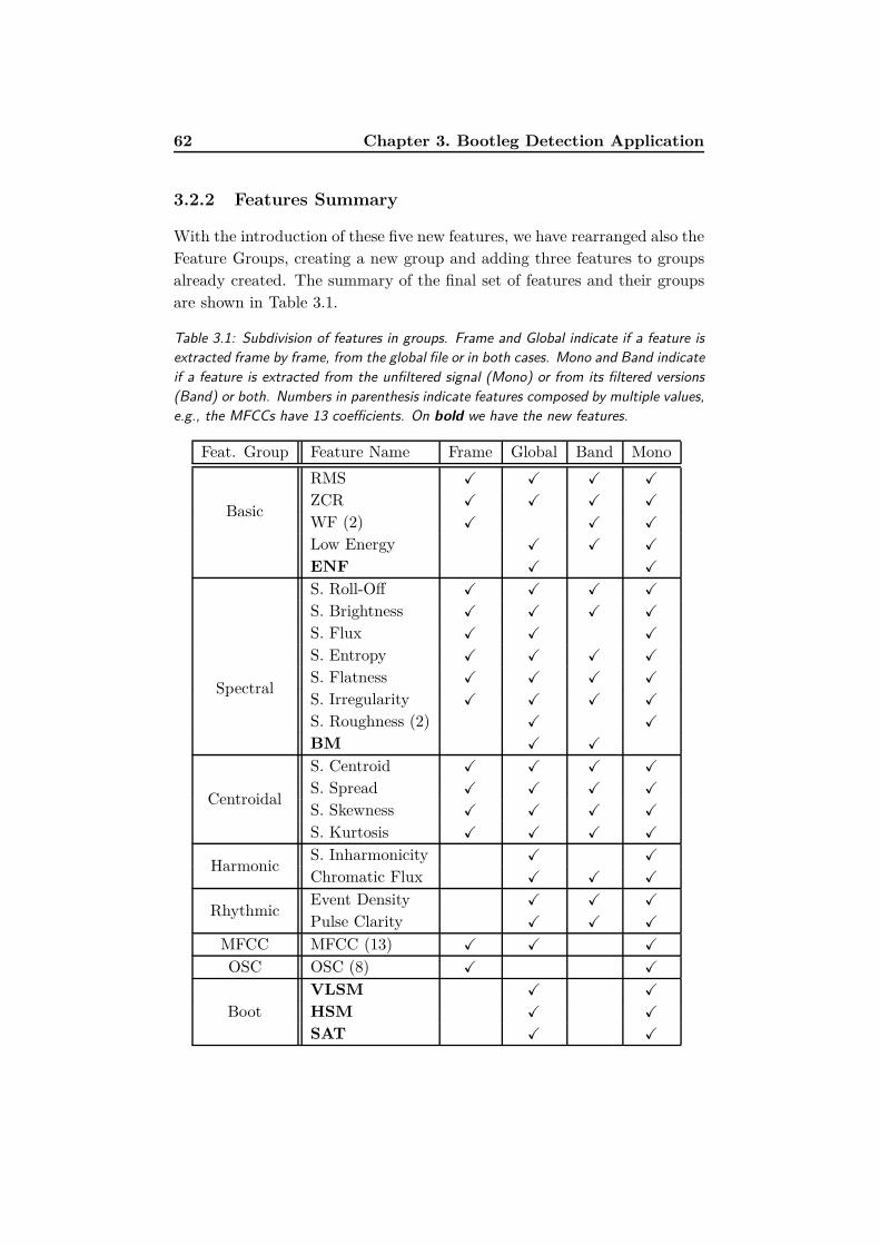
62 Chapter 3. Bootleg Detection Application
3.2.2 Features Summary
With the introduction of these five new features, we have rearranged also the
Feature Groups, creating a new group and adding three features to groups
already created. The summary of the final set of features and their groups
are shown in Table 3.1.
Table 3.1: Subdivision of features in groups. Frame and Global indicate if a feature is
extracted frame by frame, from the global file or in both cases. Mono and Band indicate
if a feature is extracted from the unfiltered signal (Mono) or from its filtered versions
(Band) or both. Numbers in parenthesis indicate features composed by multiple values,
e.g., the MFCCs have 13 coefficients. On bold we have the new features.
Feat. Group Feature Name Frame Global Band Mono
Basic
RMS X X X X
ZCR X X X X
WF (2) X X X
Low Energy X X X
ENF X X
Spectral
S. Roll-Off X X X X
S. Brightness X X X X
S. Flux X X X
S. Entropy X X X X
S. Flatness X X X X
S. Irregularity X X X X
S. Roughness (2) X X
BM X X
Centroidal
S. Centroid X X X X
S. Spread X X X X
S. Skewness X X X X
S. Kurtosis X X X X
HarmonicS. Inharmonicity X X
Chromatic Flux X X X
RhythmicEvent Density X X X
Pulse Clarity X X X
MFCC MFCC (13) X X X
OSC OSC (8) X X
Boot
VLSM X X
HSM X X
SAT X X

3.3. Bootleg Detection Feature Selection 63
3.3 Bootleg Detection Feature Selection
With the introduction of the analysis by band, we add to the previously
considered feature selection methods one that takes this band-division spe-
cifically into account. Analysing the Mono signal and the Bands we obtain
a lot of features, some of which, obviously, are more important than others.
Even if a method of feature selection is applied, some features can still be
more significant than others. Furthermore this reflection is valid for the
bands, because the analysis of some of the bands can be useless, while only
few bands can be significant. The basic idea of this method is showing how
much each band is important, removing not significant bands from the com-
putations. Moreover, some groups of features could be less significant than
others. With this method we also apply a sort of feature group weighing.
Cross-Validation Selection
We implemented a method, according to our specific problem, that allows
to assign importance weights to Bands analysed and to features groups. We
called it Cross-Validation Selection (CVS). Only the Bands and the features
with greater weights are selected, while the others are not considered. This
is done during the pre-test phase. A part of data destined to train the
machine is used as Train Set, the remaining part, called CVS Set, is used
in Pre-Test. The class membership of each file in these sets is known. After
the Pre-Test, classification accuracy is computed. Each Band is considered
separately, so the accuracy of each Band can be computed. CVS selects only
the three bands with greater weights.
Since, when we consider groups of features, we have different GMM/SVM
classifiers for each group, a metric to evaluate the performance of a single
classifier can be computed. This evaluation leads to another set of weights.
In Test Phase, a file is classified according to all the weights derived. In
the case that only the mono signal is analysed, CVS assigns only the weights
to features in the macro-sets or to the groups.
Let us see the steps of the algorithm by means of an example. For the sake
of clarity let us focus on one case. In particular let us consider the case
in which the classifier to be tested is GMM, and features are divided into
groups. For the sake of simplicity let us consider just three groups: i) basic,
ii) spectral iii) and MFCC.
1. The Train Set (TS) and the CVS Set (CS) are chosen.
2. The Train phase can start, training three GMM for each Band and for
the Mono signal:

64 Chapter 3. Bootleg Detection Application
Algorithm 7 Groups Training Steps
1: for each Band and the Mono signal do
2: Extract features from the TS
3: Train GMMBasic, GMMSpectral, GMMMF CC
4: end for
3. The Pre-Test can start, evaluating the files of CS. For each group of
features we obtain the classification result (Resultgroup), that indicates
the class membership of the file according to testing group features:
Algorithm 8 Pre-Test steps
1: for each file in CS do
2: for each band and the mono signal do
3: Extract features from the CS
4: Test CS files according to Basic, Spectral and MFCC features
ResultBasic, ResultSpectral, ResultMF CC are obtained
5: end for
6: end for
4. Considering results obtained for every file in CS, we count the number
of correctly classified files for each group (Countergroup). The accur-
acy (Accuracygroup), that is the percentage of correctly classified files
according to group features, can be computed:
Algorithm 9 Accuracy computation
1: cntCS = number of files in CS
2: for each file in CS do
3: for each band and the mono signal do
4: if ResultBasic is correct
5: CounterBasic + +
6: if ResultSpectral is correct
7: CounterSpectral + +
8: if ResultMF CC is correct
9: CounterMF CC + +
10: end for
11: end for
12: AccuracyBasic = CounterBasic/cntCS
13: AccuracySpectral = CounterSpectral/cntCS
14: AccuracyMF CC = CounterMF CC/cntCS

3.4. New Classification Phases 65
5. The Weights of each single group of features and of each Band can
now be computed.
W eightgroup indicates the weight of the feature group. W eightband is
the weight of the band. The weights are:
Algorithm 10 Weights computation
1: for each band and the mono signal do
2: W eightBasic = AccuracyBasic
3: W eightSpectral = AccuracySpectral
4: W eightMF CC = AccuracyMF CC
5: W eightBand = WeightBasic + WeightSpectral + WeightMF CC
6: end for
6. Selection of the three bands with the highest weights. The sum of the
weights of these three bands is normalized to 1.
Algorithm 11 Bands Selection
1: Select the three bands with highest weights
2: W eightT OT AL= sum of weights of the three Bands selected
3: for each of the Band selected do
4: W eightBand = W eightBand/W eightT OT AL
5: end for
In the Test phase, each band classifier associated to each group feature is
weighted according to the value of W eightgroup. For each band that isn’t
discarded, W eightBand is considered.
3.4 New Classification Phases
The Bootleg classification tool uses the same principles as the general classi-
fication tool explained in Chapter 2, but the pre-processing phase, the new
features and the new feature selection method are also considered. The clas-
sification is divided in the same three phases as the general machine: Train,
Validation and Test. We need a set of file to create the Training-Set and
the Validation-Set, that are created randomly, but in which the number of
files for each class is the same, to train the machine equally for each class.
The main difference, with respect to the work-flow previously described,
is the introduction of the features extracted from the bands. This cause a
further branching of the work-flow.

66 Chapter 3. Bootleg Detection Application
Training Phase
As in the general machine described in the previous chapter, several methods
of feature selection are used in order to find the optimal significant subset
of features that best describes the classification problem. Using the seven
types of selection methods and the new approach described before (CVS),
we have created a combination of twenty feature selection methods. With
the CVS approach, the selected features and the bands are weighted, so that
the tool uses in the test only the significant features and bands. The twenty
methods are the followings:
• NO Feature Selection applied
• Cross-Validation Selection
• Forward Feature Selection
• Forward Feature Selection + Cross-Validation Selection
• Backward Feature Selection
• Backward Feature Selection + Cross-Validation Selection
• Stepwise Feature Selection
• Stepwise Feature Selection + Cross-Validation Selection
• Genetic Algorithm
• Genetic Algorithm + Cross-Validation Selection
• RELIEF Algorithm + Forward Feature Selection
• RELIEF Algorithm + Backward Feature Selection
• Principal Component Analysis
• Principal Component Analysis + Cross-Validation Selection
• Principal Component Analysis + Forward Feature Selection
• Principal Component Analysis + Backward Feature Selection
• Principal Component Analysis + Stepwise Feature Selection
• Linear Discriminant Analysis
• Principal Component Analysis Group

3.4. New Classification Phases 67
• Principal Component Analysis Group + Cross-Validation Selection
Note that the last two methods, PCA Group and PCA Group + CVS, can
be applied only when the features are divided in groups.
Training Phase is performed in 2 ways as shown in Figure 3.7, considering
only the Mono signal or the Mono signal together with the Bands. We still
utilize one (combination of) method of feature selection/reduction at time.
In the first case, as in the general machine, a method selects the significant
features only from the Mono signal. In the second case, a method selects
a subset of features for each of the 10 Bands and the Mono signal, each of
which is used separately to train the machine.
Each preliminary division is then further subdivided in turn in other 4 cases
described in the Chapter 2 (Macro-Set or Groups of feature and then GMM
or SVM). Considering that we have 18 or 20 methods of features selection
depending on whether we analyse the features divided in groups or in Macro-
Set, in total we obtain 152 differently training for the machine (76 GMM
and 76 SVM).
Figure 3.7: Combinations of methods in the Training Phase. We obtain 152 method
combination.
The method that use the bands, but also the new features, can obviously
be used for any type of classification, and so be introduced also as modific-
ation of the general machine for purpose different from the Audio Bootleg
detection.
Validation Phase
In this phase the machine performs a Pre-test, comparing all the 152 dif-
ferent combinations with a subset of different files from the one used in the

68 Chapter 3. Bootleg Detection Application
Training-Test (and twice as large), in order to decide which one is the best.
So in the end the Validation Phase returns a 4 values decision:
• Only Mono Signal or Mono + Bands
• Macro-Set of features or Groups of features
• Best Feature Selection/Reduction Method
• Best Classifiers (GMM/SVM)
With respect to the general case described in Chapter 2, there is now the
decision about using only the Mono signal or also the Bands. When only
the Mono signal is selected, the method of combining the results of each
step is the same described in Chapter 2 in Figure 2.6. In the case when the
Bands are considered, the flow change as shown in Figure 3.8. When all
Figure 3.8: Decision merging flow in Bands + Mono case. Each Band block contains
the same sub-blocks of the Mono block.
the 10 Bands and the Mono signal are analysed, the tool has to compute
another average since each set of features, extracted from all the version of
the signal, is considered separately. So the steps are:
• average between the decisions taken for each frame (Frame Mean De-
cision);
• for each Band and for the Mono we take the average between the
Frame Mean Decision and the decision taken for the Global file, that
is the Partial Decision;

3.4. New Classification Phases 69
• average of all the Partial Decision from the Bands and the Mono to
obtain the Final Decision.
The machine is now ready to perform the test.
Test Phase
The Test Phase consists in the classification of a new file using the machine
trained with the best combination of methods obtained from the Validation
Phase. Note that, since we have specified that the CVS method may com-
pletely exclude some of the filtered version of the file as feature selection,
the number of features that are considered important may be really small.
Chapter Conclusions
In this Chapter we explained in details the proposed modification to the
classification tool, in order to best fit the bootleg classification problem. In
the next Chapter we will explain how we built the dataset, and will present
results from our tests that validate the proposed classification method.

This page is intentionally left blank.
Chapter 4
Experimental Results
In this Chapter we validate the proposed bootleg detector by means of a
wide set of experimental results. More specifically, we start from describing
the audio dataset that we built for that purpose, and then we show how we
performed the tests. Finally we analyse the obtained results, showing which
the most significant features are. This analysis confirms the hypothesis
made on the distinctive bootleg traits. Moreover, these results show that the
method proposed for combining features from different bands often obtains
the highest accuracy. For the sake of compactness, we analyse in details
only the most significant part of the results. For the complete set of test
results, see the Appendix A.
4.1 Database
The audio dataset used in the proposed work have been built exploiting
both our music library and the wide availability of music on the web.
In total we used 594 different files, split in three main categories:
• Bootleg: 264 files that fit the bootleg definition given in Chapter 3;
Home: sub-set of Bootleg, with audio excerpt expressly created at
home for our purpose.
• Official: 168 audio files recorded from live performance officially re-
leased by the artists on CDs.
• Studio: 162 audio files recorded in studio, released on CDs and taken
directly from original discs.

72 Chapter 4. Experimental Results
In general, we selected files from different musical genres, in a balanced
way. This choice has been made to avoid that the classification focuses
on a specific musical genre and not on Bootleg. While the Official and the
Studio files come directly from official supports, the Bootlegs are taken from
different sources, e.g., YouTube and sharing fans sites. We have considered
as Bootleg also 6 files obtained at a Scorpions concert. Some bands, as the
Scorpions, give at the end of the concert the recording of the performance on
USB support. These files are directly taken from the hall mixer, without any
post-processing (the support is provided instantly at the end of the concert,
there is no time to do any sort of post-processing). These files are officially
released by the artist, so technically they are not Bootleg. However, in
general, audio recorded directly from the mixer during a live performance
and without post-processing is considered as Bootleg and there are also sites
that provided the download of packages of bootleg created with this method.
Furthermore we have introduced in the Bootleg set a list of files that we have
specifically created. Bootlegs recorded with any device directly at a concert
may have high values of noisiness. The Home subset has been composed on
purpose. We have recorded some files from the Studio set, reproduced by a
home Hi-Fi and recorded with different type of microphones. We have used
7 different microphones:
• Shure professional microphone
• Nikon Coolpix (Compact Digital Camera) integrated microphone
• Nikon D5000 (Reflex Digital Camera) integrated microphone
• Dell Laptop integrated microphone
• Samsung Galaxy S2 Smart-phone integrated microphone
• Creative Zen (mp3 player) integrated microphone
• Microphone for web chat
To this purpose we have recorded 18 files for each case (they are already
included in the Bootleg total number).
In order to obtain uniform comparable files and for computational reasons,
each file consists in a minute extracted from the song considered. This
decision does not afflict the results. Furthermore, the file excerpts have been
selected to have the least possible not-musical parts. If a piece contains long
silences (parts with no music played) it is easier to observe ambient noise
such as claps or screams. If the tool had been trained with these files,
Bootleg with fewer parts of “silence” would not have been identified as such.

4.2. Experimental Test Creation 73
4.2 Experimental Test Creation
Using the database that we have created, we tested the bootleg classification
tool. We performed 10 different types of tests, considering different com-
binations of files from our database. In particular we split the database in
sub-databases, each of which has been used to test the classification tool in
a different situation. The sub-databases are divided in categories as follows:
1. All Dataset (Bootleg class A, Official+Studio class B)
2. Bootleg and Official
3. Bootleg and Studio
4. Bootleg Home Made and Corresponding Studio files
4.1 Shure Microphone and Corresponding Studio
4.2 Nikon Coolpix Microphone and Corresponding Studio
4.3 Nikon D5000 Microphone and Corresponding Studio
4.4 Dell Laptop Microphone and Corresponding Studio
4.5 Samsung Galaxy S2 Microphone and Corresponding Studio
4.6 Creative Zen Microphone and Corresponding Studio
4.7 Web Chat Microphone and Corresponding Studio
For each one of these categories, we have used 10% of the tracks as Training-
Set, the 20% of the remaining tracks within the same subset as Validation-
Set and the remaining 70% as files to be tested. This means that we have
always used a Training-Set of 60 files and a Validation-Set of 120 files. Ini-
tially, we performed tests using 10% and 30% of the Database as Training-
Set, and without any Validation Phase. Note that, in the fourth category,
Bootleg Home Made and Corresponding Studio files, we do not have enough
audio excerpts to create a Validation-Set of 60 files. In that case we have
used smaller Train and Validation sets.
Since the classification gave nearly the same results, we have decided to
use 10% of files as Training-Set and 20% of files as Validation-Set, choice
that has improved the results. From this observation, we can also affirm
that, when the number of file in the Training-Set is quite high, incrementing
the Training-Set does not improve the results. We have tested some differ-
ent files combinations with the best methods extracted from the Validation
Phase. The scope of our work is creating a tool that allows to recognizing
Audio Bootleg analysing the optimal subset of features and using the best

74 Chapter 4. Experimental Results
classifier, but we have performed tests also to demonstrate the quality of
our Validation Phase. In-fact we have performed the tests comparing all
feature selection methods and both classifiers. In this way we can show how
many Audio Bootleg files are detected, but also that the decisions made in
the Validation Phase are consistent. In Table 4.1, we show the summary of
the results obtained. For each category, accuracy and the combination of
decision after the Validation Phase are reported.
Table 4.1: Best accuracies obtained for tests of each category. Bo = Bootleg. S =
Studio. O = Official. BH = Bootleg Home Made. Corr = Corresponding Studio.
Acc = accuracy. M/Ba = Mono or Mono+Band. Gr/Mcr = Groups of features or
Macro-set of features. Class = Classifier.
Category Acc % M/Ba Gr/Mcr Feat-S Class
1. Bo vs O + S 85 Ba Mcr FWD + CVS GMM
2. Bo vs O 82 Ba Mcr FWD + CVS GMM
3. Bo vs S 89 Ba Mcr BWD + CVS GMM
4. BH vs Corr 97 Ba Gr SW + CVS GMM
5. Shure VS
Nikon Coolpix VS
Galaxy S2 VS
Corr
96 Ba Mcr FWD GMM
In Table 4.1 we have a summary of the results obtain. As we could
expect, distinguish Studio excerpts from Bootlegs is easier than any other
category of tests. This is due to the fact that Studio are the cleaner excerpts
that we have, recorded in recording studios, while Bootlegs are taken during
live performance, without any sort of cleaning post-processing. We also
expect to have lower accuracies for Bootleg and Official category, since both
sets of files are recorded during live performances.
We now analyse the results for each category of files. We also show an
analysis for some of the most significant features.
4.3 Result Statistics
We graphically show the accuracy obtained in the performed tests. We have
performed each of the 152 type of test 30 times, scrambling each times the
set of songs. In order to ensure that the obtained results are not influenced
by an ill-conditioned dataset, we average the results obtained from the 30
tests.
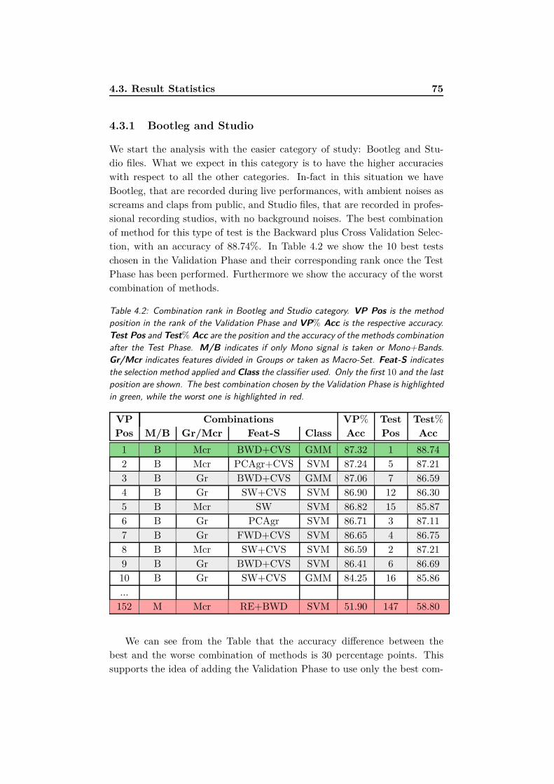
4.3. Result Statistics 75
4.3.1 Bootleg and Studio
We start the analysis with the easier category of study: Bootleg and Stu-
dio files. What we expect in this category is to have the higher accuracies
with respect to all the other categories. In-fact in this situation we have
Bootleg, that are recorded during live performances, with ambient noises as
screams and claps from public, and Studio files, that are recorded in profes-
sional recording studios, with no background noises. The best combination
of method for this type of test is the Backward plus Cross Validation Selec-
tion, with an accuracy of 88.74%. In Table 4.2 we show the 10 best tests
chosen in the Validation Phase and their corresponding rank once the Test
Phase has been performed. Furthermore we show the accuracy of the worst
combination of methods.
Table 4.2: Combination rank in Bootleg and Studio category. VP Pos is the method
position in the rank of the Validation Phase and VP% Acc is the respective accuracy.
Test Pos and Test% Acc are the position and the accuracy of the methods combination
after the Test Phase. M/B indicates if only Mono signal is taken or Mono+Bands.
Gr/Mcr indicates features divided in Groups or taken as Macro-Set. Feat-S indicates
the selection method applied and Class the classifier used. Only the first 10 and the last
position are shown. The best combination chosen by the Validation Phase is highlighted
in green, while the worst one is highlighted in red.
VP Combinations VP% Test Test%
Pos M/B Gr/Mcr Feat-S Class Acc Pos Acc
1 B Mcr BWD+CVS GMM 87.32 1 88.74
2 B Mcr PCAgr+CVS SVM 87.24 5 87.21
3 B Gr BWD+CVS GMM 87.06 7 86.59
4 B Gr SW+CVS SVM 86.90 12 86.30
5 B Mcr SW SVM 86.82 15 85.87
6 B Gr PCAgr SVM 86.71 3 87.11
7 B Gr FWD+CVS SVM 86.65 4 86.75
8 B Mcr SW+CVS SVM 86.59 2 87.21
9 B Gr BWD+CVS SVM 86.41 6 86.69
10 B Gr SW+CVS GMM 84.25 16 85.86
...
152 M Mcr RE+BWD SVM 51.90 147 58.80
We can see from the Table that the accuracy difference between the
best and the worse combination of methods is 30 percentage points. This
supports the idea of adding the Validation Phase to use only the best com-

76 Chapter 4. Experimental Results
bination of methods to perform the tests. In this case, the method selected
from the Validation has obtained the higher accuracy also in the Test Phase.
We can see that, anyway, the differences between the first ten positions are
very low. Furthermore, we can see that the best combinations use always
the features extracted from the Mono and the Bands. That means that also
the addition of the Bands has provided improvements.
In Figures 4.1 and 4.2, two 3D histograms show respectively which
are the Global and the Frame features that have been mostly selected by
BWD+CVS method and their percentage occurrences. These histograms
have been built considering the 30 test repetitions on different training set.
The shown features are a subset of all the extracted features, since the less
significant ones have already been discarded.
S.Centroid
S.Entropy
S. atnessS.Flux
S.irregularityS.Kurtosis
RmsS.Rollo!
S.SkewnessWf1
Wf2Zcr
MONO
BAND 1
BAND 2
BAND 8
BAND 9
BAND 10
0
20
40
60
80
100
Occ
urr
en
ces
(%)
Figure 4.1: Frame feature occurrences referring to Backward + Cross Validation feature
selection in Bootleg and Studio category.
Features with higher occurrences have been selected more times on the
30 tests performed, so these features are stable and not related to the com-
position of the dataset. On the contrary, features that have been selected
only few times are more related to the Training Set used. As we can see, not
all bands are shown because CVS method selects only the most significant
bands. Note that, as said in Section 3.3, the CVS method selects only the
three most significant bands. In the graph more than three bands are shown
because the best bands considered may be different in each of the 30 test.

4.3. Result Statistics 77
BM
S.Centroid
S.Flux
EvDensity
S.Rollo
S.Spread
Zcr
MONO
BAND 1
BAND 2
BAND 8
BAND 9
BAND 10
0
20
40
60
80
100
Occ
urr
en
ces
(%)
Figure 4.2: Global feature occurrences referring to Backward + Cross Validation feature
selection in Bootleg and Studio category.
Figure 4.3 shows the average weights assigned to each Band by the CVS.
Bands 9 and 10 are the most significant.
MONO BAND 1 BAND 2 BAND 3 BAND 4 BAND 5 BAND 6 BAND 7 BAND 8 BAND 9 BAND 100
0.05
0.1
0.15
0.2
0.25
0.3
0.35
AV
ER
AG
E W
EIG
HT
BA
ND
S
Figure 4.3: Percentage of weight values assigned to each Band and to the Mono signal
by the Cross Validation Selection in Bootleg and Studio category.
The same considerations on significance of the features can be done for
the features extracted only from the Mono signal (Figure 4.4). Also in this
figures only the subset of most significant features is shown.
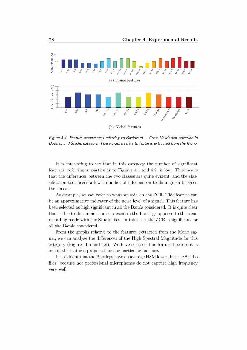
78 Chapter 4. Experimental Results
0
50
100
MFC
C9
MFC
C8
MFC
C7
MFC
C6
MFC
C5
MFC
C4
MFC
C3
MFC
C2
MFC
C13
MFC
C12
MFC
C11
MFC
C10
MFC
C1
OSC
8
OSC
7
OSC
6
OSC
5
OSC
4
OSC
3
OSC
2
OSC
1
Occ
urr
en
ces
(%)
(a) Frame features
0
20
40
60
80
100
Var
.CF
Mea
nRo
ugh
S.in
har
mon
icit
y
S.En
trop
y
MFC
C9
MFC
C5
MFC
C13
MFC
C11
MFC
C10
BM
SAT
HSM
ENF
Occ
urr
en
ces
(%)
(b) Global features
Figure 4.4: Feature occurrences referring to Backward + Cross Validation selection in
Bootleg and Studio category. These graphs refers to features extracted from the Mono.
It is interesting to see that in this category the number of significant
features, referring in particular to Figures 4.1 and 4.2, is low. This means
that the differences between the two classes are quite evident, and the clas-
sification tool needs a lower number of information to distinguish between
the classes.
As example, we can refer to what we said on the ZCR. This feature can
be an approximative indicator of the noise level of a signal. This feature has
been selected as high significant in all the Bands considered. It is quite clear
that is due to the ambient noise present in the Bootlegs opposed to the clean
recording made with the Studio files. In this case, the ZCR is significant for
all the Bands considered.
From the graphs relative to the features extracted from the Mono sig-
nal, we can analyse the differences of the High Spectral Magnitude for this
category (Figures 4.5 and 4.6). We have selected this feature because it is
one of the features proposed for our particular purpose.
It is evident that the Bootlegs have an average HSM lower that the Studio
files, because not professional microphones do not capture high frequency
very well.
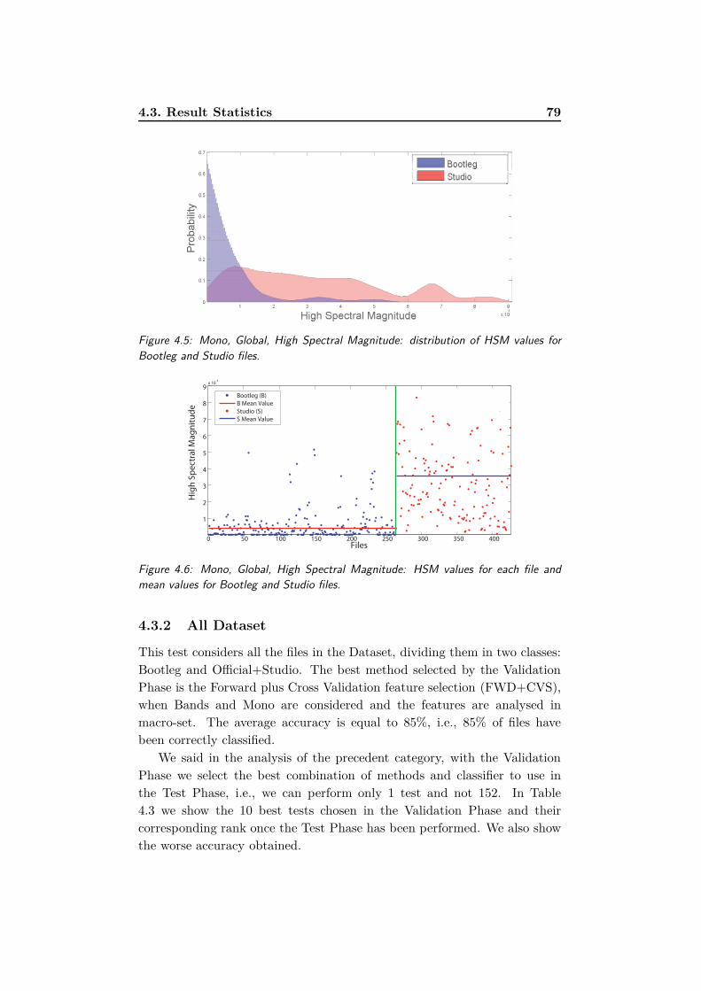
4.3. Result Statistics 79
Figure 4.5: Mono, Global, High Spectral Magnitude: distribution of HSM values for
Bootleg and Studio files.
0 50 100 150 200 250 300 350 400
1
2
3
4
5
6
7
8
9x 10
4
Files
Hig
h S
pe
ctra
l Ma
gn
itu
de
Bootleg (B)
B Mean Value
Studio (S)
S Mean Value
Figure 4.6: Mono, Global, High Spectral Magnitude: HSM values for each file and
mean values for Bootleg and Studio files.
4.3.2 All Dataset
This test considers all the files in the Dataset, dividing them in two classes:
Bootleg and Official+Studio. The best method selected by the Validation
Phase is the Forward plus Cross Validation feature selection (FWD+CVS),
when Bands and Mono are considered and the features are analysed in
macro-set. The average accuracy is equal to 85%, i.e., 85% of files have
been correctly classified.
We said in the analysis of the precedent category, with the Validation
Phase we select the best combination of methods and classifier to use in
the Test Phase, i.e., we can perform only 1 test and not 152. In Table
4.3 we show the 10 best tests chosen in the Validation Phase and their
corresponding rank once the Test Phase has been performed. We also show
the worse accuracy obtained.
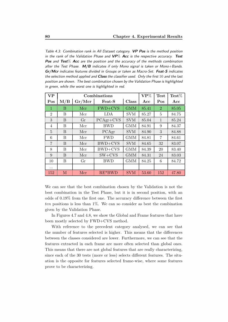
80 Chapter 4. Experimental Results
Table 4.3: Combination rank in All Dataset category. VP Pos is the method position
in the rank of the Validation Phase and VP% Acc is the respective accuracy. Test
Pos and Test% Acc are the position and the accuracy of the methods combination
after the Test Phase. M/B indicates if only Mono signal is taken or Mono+Bands.
Gr/Mcr indicates features divided in Groups or taken as Macro-Set. Feat-S indicates
the selection method applied and Class the classifier used. Only the first 10 and the last
position are shown. The best combination chosen by the Validation Phase is highlighted
in green, while the worst one is highlighted in red.
VP Combinations VP% Test Test%
Pos M/B Gr/Mcr Feat-S Class Acc Pos Acc
1 B Mcr FWD+CVS GMM 85.41 2 85.05
2 B Mcr LDA SVM 85.27 5 84.75
3 B Gr PCAgr+CVS SVM 85.04 1 85.24
4 B Mcr BWD GMM 84.91 9 84.37
5 B Mcr PCAgr SVM 84.90 3 84.88
6 B Mcr FWD GMM 84.81 7 84.61
7 B Mcr BWD+CVS SVM 84.65 32 83.07
8 B Mcr BWD+CVS GMM 84.39 20 83.40
9 B Mcr SW+CVS GMM 84.31 24 83.03
10 B Gr BWD GMM 84.25 6 84.72
...
152 M Mcr RE*BWD SVM 53.60 152 47.80
We can see that the best combination chosen by the Validation is not the
best combination in the Test Phase, but it is in second position, with an
odds of 0.19% from the first one. The accuracy difference between the first
ten positions is less than 1%. We can so consider as best the combination
given by the Validation Phase.
In Figures 4.7 and 4.8, we show the Global and Frame features that have
been mostly selected by FWD+CVS method.
With reference to the precedent category analysed, we can see that
the number of features selected is higher. This means that the differences
between the classes considered are lower. Furthermore, we can see that the
features extracted in each frame are more often selected than global ones.
This means that there are not global features that are really characterizing,
since each of the 30 tests (more or less) selects different features. The situ-
ation is the opposite for features selected frame-wise, where some features
prove to be characterizing.

4.3. Result Statistics 81
BMS.Bright
S.CentroidS. atness
S.FluxS.Irregularity
S.KurtosisEvDensity
LowEnergyPulse
RmsS.Rollo!
S.SkewnessS.Spread
Zcr
MONO
BAND 1
BAND 2
BAND 8
BAND 9
BAND 10
0
20
40
60
80
100
Occ
urr
en
ces
(%)
Figure 4.7: Percentage of occurrences of Global feature referring to Forward + Cross
Validation feature selection in All Dataset category, averaged on the 30 test performed.
S.Bright
S.Centroid
S.Entropy
S. atness
S.FluxS.irregularity
S.Kurtosis
Rms
S.Rollo!
S.Skewness
Wf1Wf2
Zcr
MONO
BAND 1
BAND 2
BAND 8
BAND 9
BAND 10
0
20
40
60
80
100
Occ
urr
en
ces
(%)
Figure 4.8: Percentage of occurrences of Frame feature referring to Forward + Cross
Validation feature selection in All Dataset category, averaged on the 30 test performed.
As we said, some features have been extracted only for the Mono signal.
We can analyse these features. Figure 4.9 shows the Global and Frame
features selected from the Mono signal with their occurrences.

82 Chapter 4. Experimental Results
0
20
40
60
80
100
Var
.CF
VLS
M
S.in
har
mon
icit
y
S.En
trop
y
MFC
C9
MFC
C5
MFC
C4
MFC
C3
MFC
C13
MFC
C12
MFC
C11
MFC
C10
HSM
ENF
Occ
urr
en
ces
(%)
(a) Global Mono feature occurrences
0
50
100
MFC
C9
MFC
C8
MFC
C7
MFC
C6
MFC
C5
MFC
C4
MFC
C3
MFC
C2
MFC
C13
MFC
C12
MFC
C11
MFC
C10
MFC
C1
OSC
8
OSC
7
OSC
6
OSC
5
OSC
4
OSC
3
OSC
2
OSC
1
Occ
urr
en
ces
(%)
(b) Frame Mono feature occurrences
Figure 4.9: Global and Frame feature occurrences referring to Forward feature selection
in All Dataset category. These graphs refer to the features extracted only for the Mono.
We have also said the CVS assign more significance only to three Bands
each time. Figure 4.10 shows the average weights assigned to each Band by
the CVS. Bands 9 and 10 are the most significant.
MONO BAND 1 BAND 2 BAND 3 BAND 4 BAND 5 BAND 6 BAND 7 BAND 8 BAND 9 BAND 100
0.05
0.1
0.15
0.2
0.25
0.3
0.35
AV
ER
AG
E W
EIG
HT
BA
ND
S
Figure 4.10: Percentage of weight values assigned to each Band and to the Mono signal
by the Cross Validation Selection in All Dataset category.
Considering only the most significant Bands, we can see that there are
features that in some Bands are more selected than in others. E.g., we can
consider the Zero Crossing Rate, that has been selected all the time in the
10-th Band. We expected the ZCR value to be higher in Bootleg files due
to some noise components. Referring to the ZCR extracted from frames of
the 10-th Band, we can analyse why this feature have been selected always
by the Forward feature selection.

4.3. Result Statistics 83
In Figure 4.11 the distribution of ZCR values is represented for bootleg e
not-bootleg files.
Figure 4.11: Band 10, Frame, Zero Crossing Rate: distribution of ZCR values for
Bootleg and not-Bootleg files.
As we can see, most of Bootleg files have a high ZCR value, while most of
not-Bootleg files have a lower value. Figure 4.12 shows the values of the
ZCR for each file and its mean value for Bootleg and not-Bootleg.
0 100 200 300 400 500
3.2
3.3
3.4
3.5
3.6
3.7
3.8
3.9
x 104
Files
Ze
ro C
ross
ing
Ra
te
Bootleg (B)
B Mean Value
O!cial+Studio (OS )
OS Mean Value
Figure 4.12: Band 10, Frame, Zero Crossing Rate: ZCR values for each file and value
means for Bootleg and not-Bootleg files.
From these two figures is quite clear that the distribution of values of this
feature is very different in the two classes. This means that the ZCR (espe-
cially for the considered Band) is very characterizing.
We can analyse also from the Mono signal one of the most significant
feature. We show as example the Electrical Network Frequency, that is one
of the feature added in Chapter 3 for the Bootleg Detection problem. The
ENF shows a high value when some post-processing has been applied to a
file. In Figure 4.13, we show the distribution of Electrical Network Frequency

84 Chapter 4. Experimental Results
values. We make some considerations about the ENF distribution. In rare
cases, Bootlegs are recorded with device connected to the electricity network,
so the ENF value of Bootleg files is lower. Furthermore, is probable that
the higher cleanness of Studio files permit to individuate more easily jitters
(not necessarily bounded to the electrical network) around the 50 Hz, and
so the ENF values of Studio files is higher.
Figure 4.13: Mono, Global, Electrical Network Frequency: distribution of ENF values
for Bootleg and not-Bootleg files.
As for the ZCR, in Figure 4.14 ENF values of each file and the means of the
two separated classes are represented.
0 100 200 300 400 500
500
1000
1500
2000
2500
3000
Files
Ele
ctri
cal N
etw
ork
Fre
qu
en
cy
Bootleg (B)
B Mean Value
O!cial+Studio (OS)
OS Mean Value
Figure 4.14: Mono, Global, Electrical Network Frequency: ENF values for each file and
value means for Bootleg and not-Bootleg files.

4.3. Result Statistics 85
4.3.3 Bootleg and Official
In the first category analysed, we have considered Bootleg and Studio files.
The Studio files have, obviously, less noise both of the Bootleg and the
Official ones. We have so performed these tests, to obtain results with only
live excerpt, where there is the presence of ambient noise (clasp, scream,
etc.). We expect to have results lower than the Bootleg and Official category.
Anyway, we obtained an average accuracy percentage of 81.80% in the best
case (Forward Feature Selection), that is only 3% percentage points less than
the All Dataset category. In Table 4.4, as done for precedent categories, we
show the different accuracies between Validation and Test phases.
Table 4.4: Combination rank in Bootleg and Official category. VP Pos is the method
position in the rank of the Validation Phase and VP% Acc is the respective accuracy.
Test Pos and Test% Acc are the position and the accuracy of the methods combination
after the Test Phase. M/B indicates if only Mono signal is taken or Mono+Bands.
Gr/Mcr indicates features divided in Groups or taken as Macro-Set. Feat-S indicates
the selection method applied and Class the classifier used. Only the first 10 and the last
position are shown. The best combination chosen by the Validation Phase is highlighted
in green, while the worst one is highlighted in red.
VP Combinations VP% Test Test%
Pos M/B Gr/Mcr Feat-S Class Acc Pos Acc
1 B Mcr FWD+CVS SVM 83.70 3 81.80
2 B Gr PCA SVM 83.30 2 82.00
3 B Mcr PCAgr SVM 83.10 1 82.50
4 B Gr GA GMM 82.90 9 81.30
5 B Mcr LDA GMM 82.00 16 80.80
6 B Mcr SW GMM 81.90 10 81.10
7 B Gr GA+CVS GMM 81.80 18 80.60
8 B Gr LDA SVM 81.70 6 81.60
9 B Gr SW+CVS GMM 81.50 9 81.30
10 B Mcr SW+CVS SVM 81.40 4 81.70
...
152 M Mcr RE+FWD SVM 49.90 152 50.80
We show the significant feature for this case in Figure 4.15 and Figure
4.16. The main consideration about specific features and bands weights are
more or less the same that we have done before. Indeed, the most significant
features (i.e., those with many occurrences) are those computed frame-wise
and finally aggregated.

86 Chapter 4. Experimental Results
S.BrightS.Centroid
S.EntropyS. atness
S.FluxS.irregularity
S.KurtosisRms
S.Rollo!S.Skewness
Wf1Wf2
ZcrMONO
BAND 1
BAND 2
BAND 3
BAND 7
BAND 8
BAND 9
BAND 10
0
20
40
60
80
100
Occ
urr
en
ces
(%)
Figure 4.15: Frame feature occurrences referring to Forward + Cross Validation selec-
tion in Bootleg and Official category.
BMS.Bright
S.CentroidS. atness
S.FluxS.Irregularity
S.KurtosisEvDensity
LowEnergyPulse
RmsS.Rollo!
S.SkewnessS.Spread
Zcr
MONO
BAND 1
BAND 2
BAND 3
BAND 7
BAND 8
BAND 9
BAND 10
0
20
40
60
80
100
Occ
urr
en
ces
(%)
Figure 4.16: Global feature occurrences referring to Forward + Cross Validation selec-
tion in Bootleg and Official category.
Anyway, we can show an example of significant feature for these tests. In
figure 4.17 we show the values of the Band Magnitude of each signal for the
Band 9. As we can see, the Bootlegs have lower values of Band Magnitude

4.3. Result Statistics 87
respect to the Officials. This can be the consequences of a band-pass filter
present in the integrated microphones, that cuts the higher frequencies.
0 50 100 150 200 250 300 350 4000
200
400
600
800
1000
1200
Files
Ba
nd
Ma
gn
itu
de
Bootleg (B)
B Mean Value
O!cial (O)
O Mean Value
Figure 4.17: Values of the Band Magnitude of each file for Band 9 and relative average
for Bootlegs and Officials.
As for the precedent categories, we can see in the end the feature occur-
rences for features extracted only from Mono signal (Figure 4.18).
0
50
100
MFC
C9
MFC
C8
MFC
C7
MFC
C6
MFC
C5
MFC
C4
MFC
C3
MFC
C2
MFC
C13
MFC
C12
MFC
C11
MFC
C10
MFC
C1
OSC
8
OSC
7
OSC
6
OSC
5
OSC
4
OSC
3
OSC
2
OSC
1
Occ
urr
en
ces
(%)
(a) Frame features
0
50
100
Var
.CF
Mea
nRo
ugh
Mea
n.C
F
VLS
M
S.in
har
mon
icit
y
S.En
trop
y
MFC
C9
MFC
C8
MFC
C7
MFC
C6
MFC
C5
MFC
C4
MFC
C3
MFC
C2
MFC
C13
MFC
C12
MFC
C11
MFC
C10
MFC
C1
BM
HSM
ENF
Occ
urr
en
ces
(%)
(b) Global features
Figure 4.18: Global and Frame feature occurrences referring to Forward feature selection
in Bootleg and Official category. These graphs refer to the features extracted only for
the Mono.
4.3.4 Multi-class Results Example
We analyse now another significant category of tests. In this case we try a
4-class classification, utilising home-made bootlegs. We compare here three
home-made categories with their corresponding studio versions. The best
combination of method for these type of test is the Forward feature selection,

88 Chapter 4. Experimental Results
with an accuracy of 97%. In this case all Bands are analysed. We can deduce
that this test case is more oriented to microphone source detection.
In Table 4.5, we show the 10 best tests chosen in the Validation Phase
and their corresponding rank once the Test Phase has been performed.
Table 4.5: Combination rank in Multi-class category. VP Pos is the method position
in the rank of the Validation Phase and VP% Acc is the respective accuracy. Test
Pos and Test% Acc are the position and the accuracy of the methods combination
after the Test Phase. M/B indicates if only Mono signal is taken or Mono+Bands.
Gr/Mcr indicates features divided in Groups or taken as Macro-Set. Feat-S indicates
the selection method applied and Class the classifier used. Only the first 10 and the last
position are shown. The best combination chosen by the Validation Phase is highlighted
in green, while the worst one is highlighted in red.
VP Combinations VP% Test Test%
Pos M/B Gr/Mcr Feat-S Class Acc Pos Acc
1 B Mcr FWD GMM 95.83 1 95.83
2 B Mcr BWD SVM 95.83 2 94.44
3 B Mcr PCAgr SVM 95.83 3 94.44
4 B Mcr PCAgr+CVS SVM 94.44 6 93.06
5 B Mcr SW GMM 94.44 11 90.28
6 B Mcr LDA GMM 94.44 7 93.06
7 B Gr BWD SVM 93.06 4 94.44
8 B Gr LDA SVM 93.06 5 94.44
9 B Gr SW GMM 88.89 8 93.06
10 B Mcr FWD GMM 88.89 16 88.89
...
152 M Mcr RE*BWD GMM 17.20 148 19.10
We can see from Figure 4.19 that also in the Multi-class category some
features are quite different between classes, and so are significant.
As we can see in Figure 4.20 and in Figure 4.21, fewer features are
selected. However, CVS is not used, so all Bands are considered. The
reason is the need to analyse all bands in order to distinguish 4 classes.
In Figure 4.22 frame features extracted from Mono signal are shown.
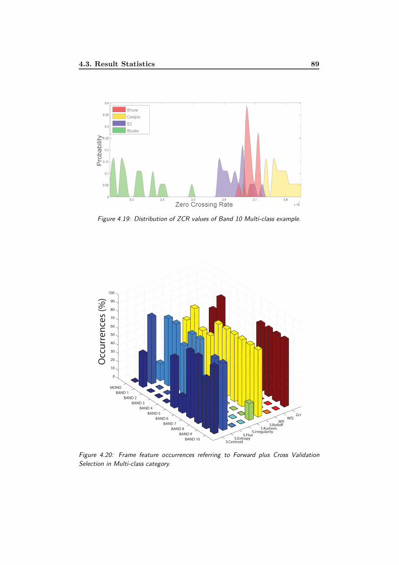
4.3. Result Statistics 89
Figure 4.19: Distribution of ZCR values of Band 10 Multi-class example.
S.CentroidS.Entropy
S.FluxS.irregularity
S.KurtosisS.Rollo
Wf1Wf2
Zcr
MONO
BAND 1
BAND 2
BAND 3
BAND 4
BAND 5
BAND 6
BAND 7
BAND 8
BAND 9
BAND 10
0
10
20
30
40
50
60
70
80
90
100
Occ
urr
en
ces
(%)
Figure 4.20: Frame feature occurrences referring to Forward plus Cross Validation
Selection in Multi-class category.

90 Chapter 4. Experimental Results
BMS.Centroid
S.FluxEvDensity
S.Rollo S.Spread
Zcr
MONO
BAND 1
BAND 2
BAND 3
BAND 4
BAND 5
BAND 6
BAND 7
BAND 8
BAND 9
BAND 10
0
10
20
30
40
50
60
70
80
90
100
Occ
urr
en
ces
(%)
Figure 4.21: Global feature occurrences referring to Forward plus Cross Validation
Selection in Multi-class category.
0
20
40
60
80
100
MFC
C9
MFC
C8
MFC
C7
MFC
C6
MFC
C5
MFC
C4
MFC
C3
MFC
C2
MFC
C13
MFC
C12
MFC
C10
MFC
C1
OSC
1 O
ccu
rre
nce
s (%
)
Figure 4.22: Frame feature occurrences referring to Forward feature selection in Multi-
class category. These graphs refer to the features extracted only for the Mono.

4.3. Result Statistics 91
4.3.5 Bootlegs Home Made and Corresponding Studio Files
In the end, since we have re-recorded some files at home, we have done some
tests between the original excerpts and their re-captured version. As said in
Section 4.1, we created the Home Made Bootlegs re-capturing with different
microphones some Studio excerpts. We have performed tests considering
only excerpts recorded by one microphone at time. We so expected to have
an high accuracy, since one class contains only audio tracks recorded with
the same device. Indeed, we can see from Table 4.6 that the accuracies are
very high.
Table 4.6: Combination rank in Home-Made Bootlegs and Corresponding Studio Files.
VP Pos is the method position in the rank of the Validation Phase and VP% Acc is the
respective accuracy. Test Pos and Test% Acc are the position and the accuracy of the
methods combination after the Test Phase. M/B indicates if only Mono signal is taken
or Mono+Bands. Gr/Mcr indicates features divided in Groups or taken as Macro-Set.
Feat-S indicates the selection method applied and Class the classifier used. Only the
first 10 and the last position are shown. The best combination chosen by the Validation
Phase is highlighted in green, while the worst one is highlighted in red.
VP Combinations VP% Test Test%
Pos M/B Gr/Mcr Feat-S Class Acc Pos Acc
1 B Gr SW+CVS GMM 97.22 1 97.22
2 B Mcr FWD+CVS GMM 97.22 3 97.22
3 B Gr PCAgr+CVS SVM 97.22 2 97.22
4 B Gr BWD+CVS GMM 97.22 5 94.44
5 B Gr FWD+CVS GMM 94.44 4 94.44
6 B Mcr LDA GMM 94.44 3 94.44
7 B Mcr GA+CVS GMM 94.44 7 94.44
8 B Gr GA+CVS GMM 94.44 8 94.44
9 B Mcr SW+CVS GMM 94.44 9 94.44
10 B Gr PCAgr SVM 94.44 10 94.44
...
152 M Mcr RE*FWD GMM 43.80 148 65.40
Chapter Conclusions
In this Chapter we have shown the results related to our work. We can
observe some constant and interesting conclusions.
First of all, the tests with the higher accuracies consider always both the

92 Chapter 4. Experimental Results
Mono signal and the Bands. This means that, for our specific purpose,
information extracted from particular sections of frequencies are more rel-
evant than information extracted from the not-processed file. Furthermore
we can observe that not all the Bands carry relevant information. In-fact
only some Bands are considered from our Cross Validation selection and,
in general, features derived from the extreme bands have higher weights.
The lower Bands (1 and 2) and the higher Bands (8, 9 and 10) are the most
considered. The central Bands from 3 to 7 are never considered. This means
that the central frequencies (from 230 Hz to 8 kHz) do not carry relevant
information, or probably that the information carried by these Bands are
the same retrieved from the Mono signal.
We have obtained a high accuracy of Bootleg detection in every category
of test (i.e., higher than 80%). In particular, as we expected, experimental
results show that some features characterize bootlegs much better than oth-
ers. Among these, we found that features that capture noise characteristics
(such as ZCR, ENF or features related to high-frequency bands) can be
essential to solve the problem.
Analysing the results that we obtained, we can conclude that the low-
est and the highest considered frequency bands are the most significant to
solve the bootleg detection problem. The importance of the low frequencies
analysis is explained by the rumbling phenomenon, i.e., an excess of low
frequency noise that can be present in a recording environment. On the
other hand, recording an audio track in a particularly crowdy place (typ-
ical of concert halls) may give rise to a high frequency absorption. This
phenomenon is given by the reflections, refractions and diffractions due to
the presence of the bodies of people that cause a sort of confusion in the
registration. For this reason, high frequency components in a bootleg may
result less clear than in studio songs.

Chapter 5
Conclusions and Future
works
In this work we presented a method to solve the audio bootleg detection
problem, which is a problem of interest in the forensic community. Indeed,
with the increasing diffusion of portable recording devices, such as integrated
microphones in photo-cameras, mp3 players and many more, it is nowadays
easy for everyone to create and share bootlegs. For this reason, a tool that
allows to automatically detect bootlegs may be helpful to prevent copyright
infringements, e.g., on multimedia sharing platforms.
The detector that we propose starts from a classification tool that is as
general and modular as possible. It is based on audio features extraction
and classifiers such as GMMs and SVMs. However, additional features, fea-
tures selection methods, and classifiers can be added at any moment. The
classification procedure that we propose is then developed to automatically
select the best combination of features and classifiers to maximize the clas-
sification accuracy using a small set of training data and comparing many
different feature selection methods.
To tune this tool in order to solve the bootleg detection problem, we
have considered an additional set of features and a feature selection method
that allows fusing information from different frequency bands of the signal.
To test the detector, we have built a Dataset of nearly 600 audio excerpts.
We have divided the Dataset in Bootleg, Home Made Bootleg, Official and
Studio excerpts. Bootlegs are files obtained mainly from the web, they are
illegally distributed. Home Made Bootlegs are excerpts created on purpose
re-capturing some original Studio-recorded audio. Officials and Studios are
files officially release by artists, respectively recorded in live performances
94 Chapter 5. Conclusions and Future works
and in recording studios. By using such different audio excerpts, we have
been able to test the tool in different situations, obtaining a high accuracy
of Bootleg detection in every case (i.e., higher than 80%). In particular,
as we expected, experimental results show that some features characterize
bootlegs much better than others. Among these, we found that features
that capture noise characteristics (such as ZCR or features related to high-
frequency bands) can be essential to solve the problem.
Even if results are promising, the detector could still be improved. As an
example, a set of high-level features could be inserted into the pool of tested
features. Moreover, more in depth studies on the presence of characteristic
reverberations on bootlegs could be carried on to improve the robustness
of the detector. Another idea could be the texture analysis of the chroma-
gram. Indeed, we used the chromagram as a feature without any processing.
However, using it as a picture and compute a feature that characterizes its
texture could be an interesting addition.
From a slightly different point of view, another interesting future work
may be the study of an anti-forensic technique. Indeed, since it is now pos-
sible to discriminate between bootlegs and non-bootlegs, it would interesting
to analyse the possibility of fooling this detector applying some kinds of au-
dio post-processing operations aiming to remove bootlegs footprints without
affecting the sound quality.

Bibliography
[1] S. Milani, M. Fontani, P. Bestagini, M. Barni, A. Piva, M. Tagliasacchi,
and S. Tubaro. An overview on video forensics. APSIPA Transactions
on Signal and Information Processing, 1:2–15, 11 2012.
[2] R. Maher. Audio forensic examination. Signal Processing Magazine,
IEEE, 26(2):84–94, 2009.
[3] T. Thongkamwitoon, H. Muammar, and P. L. Dragotti. Identification
of image acquisition chains using a dictionary of edge profiles. In Sig-
nal Processing Conference (EUSIPCO), 2012 Proceedings of the 20th
European, pages 1757–1761, 2012.
[4] J. Lukas, J. Fridrich, and M. Goljan. Digital camera identification
from sensor pattern noise. Information Forensics and Security, IEEE
Transactions on, 1(2):205–214, 2006.
[5] C. Mo, J. Fridrich, M. Goljan, and J. Lukas. Determining image origin
and integrity using sensor noise. Information Forensics and Security,
IEEE Transactions on, 3(1):74–90, 2008.
[6] F. Wang and H. Farid. Detecting re-projected video. In Kaushal So-
lanki, Kenneth Sullivan, and Upamanyu Madhow, editors, Information
Hiding, volume 5284 of Lecture Notes in Computer Science, pages 72–
86. Springer Berlin Heidelberg, 2008.
[7] M. Visentini Scarzanella and P. L. Dragotti. Video jitter analysis for
automatic bootleg detection. In Multimedia Signal Processing (MMSP),
2012 IEEE 14th International Workshop on, pages 101 –106, sept. 2012.
[8] R. Buchholz, C. Kraetzer, and J. Dittmann. Microphone classification
using fourier coefficients. In Information Hiding, pages 235–246, 2009.
[9] H. Malik and H. Farid. Audio forensics from acoustic reverberation. In
Acoustics Speech and Signal Processing (ICASSP), 2010 IEEE Inter-
national Conference on, pages 1710–1713, 2010.
95
96 BIBLIOGRAPHY
[10] N. Peters, H. Lei, and G. Friedland. Name that room: room identi-
fication using acoustic features in a recording. In ACM International
Conference on Multimedia Retrieval (ICMR), 2012 20th ACM interna-
tional conference on, MM ’12, pages 841–844, New York, NY, USA,
2012. ACM.
[11] G. Tzanetakis and P. Cook. Musical genre classification of audio sig-
nals. Acoustics Speech and Signal Processing (ICASSP), 2002 IEEE
International Conference on, 10(5):293 – 302, jul 2002.
[12] L. Chiarandini, M. Zanoni, and A. Sarti. A system for dynamic playlist
generation driven by multimodal control signals and descriptors. In
Multimedia Signal Processing (MMSP), 2011 IEEE 13th International
Workshop on, pages 1–6, 2011.
[13] D. Venkatraman and A. Makur. A compressive sensing approach to
object-based surveillance video coding. In Acoustics Speech and Sig-
nal Processing (ICASSP), 2009 IEEE International Conference, pages
3513–3516, 2009.
[14] W. S. Lin, S. K. Tjoa, H. V. Zhao, and K. J. R. Liu. Digital image
source coder forensics via intrinsic fingerprints. Information Forensics
and Security, IEEE Transactions on, 4(3):460–475, 2009.
[15] Z. Fan and R.L. de Queiroz. Identification of bitmap compression his-
tory: Jpeg detection and quantizer estimation. Image Processing, IEEE
Transactions on, 12(2):230–235, 2003.
[16] S. Chu, S. Narayanan, and C. Kuo. Environmental sound recogni-
tion with time-frequency audio features. Acoustics Speech and Sig-
nal Processing (ICASSP), 2010 IEEE International Conference on,
17(6):1142–1158, 2010.
[17] L. Gerosa, G. Valenzise, F. Antonacci, M. Tagliasacchi, and A. Sarti.
Scream and gunshot detection in noisy environments. In EURASIP
European Signal Processing Conference (EUSIPCO), 2007.
[18] S. De, I. Roy, T. Prabhakar, K. Suneja, S. Chaudhuri, R. Singh, and
B. Raj. Plagiarism detection in polyphonic music using monaural signal
separation. In Interspeech. ISCA, 2012.
[19] G. Peeters. A large set of audio features for sound description (similarity
and classification) in the cuidado project. Tech. rep., IRCAM, 2004.

BIBLIOGRAPHY 97
[20] B. Kedem. Spectral analysis and discrimination by zero-crossings. Pro-
ceedings of the IEEE, 74(11):1477 – 1493, nov. 1986.
[21] K. Jensen. Sound Examples: Timbre Models of Musical Sounds. Rap-
port (Københavns universitet. Datalogisk institut). Kobenhavns Uni-
versitet, Datalogisk Institut, 1999.
[22] R. Plomp and W. J. Levelt. Tonal consonance and critical bandwidth.
The Journal of the Acoustical Society of America, 38(4):548–560, Oc-
tober 1965.
[23] L. Olivier and T. Petri. Mir in matlab (ii): A toolbox for musical
feature extraction from audio. In ISMIR 2007, pages 127–130, 2007.
[24] W. A. Sethares. Tuning Timbre Spectrum Scale. Springer, 1 edition,
January 1998.
[25] J. M. Grey and J. W. Gordon. Perceptual effects of spectral modi-
fications on musical timbres. The Journal of the Acoustical Society of
America, 63(5):1493–1500, 1978.
[26] E. Scheirer and M. Slaney. Construction and evaluation of a robust
multifeature speech/music discriminator. In Acoustics Speech and Sig-
nal Processing (ICASSP), 1997 IEEE International Conference on,
volume 2, pages 1331 –1334 vol.2, apr 1997.
[27] L. Olivier, E. Tuomas, T. Petri, and F. Jose. Multi-feature modeling
of pulse clarity: Design, validation and optimization. In Juan Pablo
Bello, Elaine Chew, and Douglas Turnbull, editors, ISMIR 2008, 9th
International Conference on Music Information Retrieval, pages 521–
526, 2008.
[28] C. H. Lee, J. L. Shih, K. M. Yu, and H. S. Lin. Automatic music
genre classification based on modulation spectral analysis of spectral
and cepstral features. Multimedia, IEEE Transactions on, 11(4):670
–682, june 2009.
[29] B. N. Jiang, L. Lu, H. J. Zhang, J. H. Tao, and L. H. Cai. Music
type classification by spectral contrast feature. In Multimedia and Expo
(ICME), 2002 IEEE International Conference on, volume 1, pages 113
– 116 vol.1, 2002.
[30] D. Michie, D. Spiegelhalter, C. Taylor, and J. Campbell. Machine
learning, neural and statistical classification. Ellis Horwood, Upper
Saddle River, NJ, USA, 1994.

98 BIBLIOGRAPHY
[31] P. Paalanen. Bayesian classification using gaussian mixture model and
em estimation: Implementations and comparisons. Technical report,
Information Technology Project„ 2004.
[32] W. H. Press, S. A. Teukolsky, W. T. Vetterling, and B. P. Flannery.
Numerical Recipes 3rd Edition: The Art of Scientific Computing. Cam-
bridge University Press, New York, NY, USA, 3 edition, 2007.
[33] F. Yan and Q. Huijing, D.and Yanzhou. A study of audio classification
on using different feature schemes with three classifiers. In Information
Networking and Automation (ICINA), 2010 International Conference
on, volume 1, pages V1–298 –V1–302, oct. 2010.
[34] T. Hastie, R. Tibshirani, and J. Friedman. The Elements of Statist-
ical Learning: Data Mining, Inference, and Prediction, Second Edi-
tion. Springer Series in Statistics. Springer, 0002-2009. corr. 3rd edition,
September 2009.
[35] L. Burrell, O. Smart, G. J. Georgoulas, E. Marsh, and G. J. Vacht-
sevanos. Evaluation of feature selection techniques for analysis of func-
tional mri and eeg. In Dmin, pages 256–262, 2007.
[36] Z. Li, J. Zheng, F. Wang, X. Li, B. Ai, and J. Qian. A genetic algorithm
based wrapper feature selection method for classification of hyperspec-
tral images using support vector machine. The International Archives
of the Photogrammetry, Remote Sensing and Spatial Information Sci-
ences, Vol. XXXVII:Part B7, 2008.
[37] P.Y. Xia, X.Q. Ding, and B. Jiang. A ga-based feature selection and en-
semble learning for high-dimensional datasets. In Machine Learning and
Cybernetics (ICMLC), 2009 International Conference on, volume 1,
pages 7–12, 2009.
[38] J. Bins and B.A. Draper. Feature selection from huge feature sets. In
Computer Vision (ICCV), 2001 8th IEEE International Conference on,
volume 2, pages 159 –165 vol.2, 2001.
[39] K. Kira and L. A. Rendell. The feature selection problem: traditional
methods and a new algorithm. In Proceedings of the tenth national
conference on Artificial intelligence, AAAI’92, pages 129–134. AAAI
Press, 1992.
[40] T. Jehan and T. Machover. Creating Music by Listening. PhD thesis,
Massachusetts Institute of Technology, 2005.

BIBLIOGRAPHY 99
[41] A. J. Eronen, V. T. Peltonen, J. T. Tuomi, A. P. Klapuri, S. Fagerlund,
T. Sorsa, G. Lorho, and J. Huopaniemi. Audio-based context recogni-
tion. Acoustics Speech and Signal Processing (ICASSP), 2006 IEEE
International Conference on, 14(1):321 – 329, jan. 2006.
[42] S. Mika, G. Ratsch, J. Weston, B. Scholkopf, and K. Muller. Fisher
discriminant analysis with kernels. In Neural Networks for Signal Pro-
cessing IX, 1999. Proceedings of the 1999 IEEE Signal Processing So-
ciety Workshop., pages 41–48, 1999.
[43] Y. Yaslan and Z. Cataltepe. Audio music genre classification using dif-
ferent classifiers and feature selection methods. In Pattern Recognition
(ICPR), 2006 18th International Conference on, volume 2, pages 573
–576, 0-0 2006.
[44] G. Muhammad and K. Alghathbar. Environment recognition from au-
dio using mpeg-7 features. In Embedded and Multimedia Computing
(EMC), 2009 4th International Conference on, pages 1 –6, dec. 2009.
[45] J. Kaiser. System Analysis by Digital Computer. J. Wiley, 1967.
[46] D. P. Nicolalde and J. A. Apolinario. Evaluating digital audio authen-
ticity with spectral distances and enf phase change. In Acoustics Speech
and Signal Processing (ICASSP), 2009 IEEE International Conference
on, pages 1417–1420, 2009.

This page is intentionally left blank.
Appendix A
Other Test Results
We show now some other graphs relative to tests described in Chapter 4.
We can see, in the following histograms, the accuracies related to all the 152
combinations of methods for each category of test. For each category, the
first two graphs indicate the case where only Mono signal in considered, and
respectively where the features are analysed in Macro-set and in Groups.
The last two indicate the case where Mono signal and Bands are considered,
respectively with the features analysed in Macro-set and in Groups.
A.1 Bootleg and Studio
In this category of tests we consider Bootleg and Studio excerpts. We have
Bootleg, that are recorded during live performances, with ambient noises
as screams and claps from public, and Studio files, that are recorded in
professional recording studios, with no background noises.

102 Appendix A. Other Test Results
0
20
40
60
80
100
AC
CU
RA
CY
(%
)
NO
F.S
.
CV
S
FWD
FWD
+ C
VS
BW
DB
WD
+ C
VS SW
SW +
CV
S GA
GA
+ C
VS
RE
+ F
WD
RE
+ B
WD
PCA
PCA
+ C
VS
PCA
+ F
WD
PCA
+ B
WD
PCA
+ S
W LDA
PCA
Gro
up
PCA
Gro
up
+ C
VS
GMM
SVM
(a) Features divided in groups
0
10
20
30
40
50
60
70
80
90
100
AC
CU
RA
CY
(%
)
NO
F.S
.
CV
S
FWD
FWD
+ C
VS
BW
DB
WD
+ C
VS SW
SW +
CV
S GA
GA
+ C
VS
RE
+ F
WD
RE
+ B
WD
PCA
PCA
+ C
VS
PCA
+ F
WD
PCA
+ B
WD
PCA
+ S
W
LDA
GMM
SVM
(b) Macro-set of features
Figure A.1: Test results for Bootleg and Studio category: accuracy for each (combin-
ation of) method of feature selection/reduction both for GMM and SVM classifiers.
Only features from the Mono signal are used.

A.1. Bootleg and Studio 103
0
20
40
60
80
100
AC
CU
RA
CY
(%
)
NO
F.S
.
CV
S
FWD
FWD
+ C
VS
BW
DB
WD
+ C
VS SW
SW +
CV
S GA
GA
+ C
VS
RE
+ F
WD
RE
+ B
WD
PCA
PCA
+ C
VS
PCA
+ F
WD
PCA
+ B
WD
PCA
+ S
W
LDA
PCA
Gro
up
PCA
Gro
up
+ C
VS
GMM
SVM
(a) Features divided in groups
0
10
20
30
40
50
60
70
80
90
100
AC
CU
RA
CY
(%
)
NO
F.S
.
CV
S
FWD
FWD
+ C
VS
BW
DB
WD
+ C
VS
SW
SW +
CV
S GA
GA
+ C
VS
RE
+ F
WD
RE
+ B
WD
PCA
PCA
+ C
VS
PCA
+ F
WD
PCA
+ B
WD
PCA
+ S
W
LDA
GMM
SVM
(b) Macro-set of features
Figure A.2: Test results for Bootleg and Studio category: accuracy for each (combin-
ation of) method of feature selection/reduction both for GMM and SVM classifiers.
Features both from Band and Mono signal are used.

104 Appendix A. Other Test Results
A.2 All Dataset
This test considers all the files in the Dataset, dividing them in two classes:
Bootleg and Official+Studio.
0
20
40
60
80
100
AC
CU
RA
CY
(%
)
NO
F.S
.
CV
S
FWD
FWD
+ C
VS
BW
DB
WD
+ C
VS SW
SW +
CV
S GA
GA
+ C
VS
RE
+ F
WD
RE
+ B
WD
PCA
PCA
+ C
VS
PCA
+ F
WD
PCA
+ B
WD
PCA
+ S
W LDA
PCA
Gro
up
PCA
Gro
up
+ C
VS
GMM
SVM
(a) Features divided in groups
0
10
20
30
40
50
60
70
80
90
100
AC
CU
RA
CY
(%
)
NO
F.S
.
CV
S
FWD
FWD
+ C
VS
BW
DB
WD
+ C
VS SW
SW +
CV
S GA
GA
+ C
VS
RE
+ F
WD
RE
+ B
WD
PCA
PCA
+ C
VS
PCA
+ F
WD
PCA
+ B
WD
PCA
+ S
W LDA
GMM
SVM
(b) Macro-set of features
Figure A.3: Test results for All Dataset category: accuracy for each (combination
of) method of feature selection/reduction both for GMM and SVM classifiers. Only
features from the Mono signal are used.

A.2. All Dataset 105
0
20
40
60
80
100
AC
CU
RA
CY
(%
)
NO
F.S
.
CV
S
FWD
FWD
+ C
VS
BW
DB
WD
+ C
VS SW
SW +
CV
S GA
GA
+ C
VS
RE
+ F
WD
RE
+ B
WD
PCA
PCA
+ C
VS
PCA
+ F
WD
PCA
+ B
WD
PCA
+ S
W LDA
PCA
Gro
up
PCA
Gro
up
+ C
VS
GMM
SVM
(a) Features divided in groups
0
10
20
30
40
50
60
70
80
90
100
AC
CU
RA
CY
(%
)
NO
F.S
.
CV
S
FWD
FWD
+ C
VS
BW
DB
WD
+ C
VS SW
SW +
CV
S GA
GA
+ C
VS
RE
+ F
WD
RE
+ B
WD
PCA
PCA
+ C
VS
PCA
+ F
WD
PCA
+ B
WD
PCA
+ S
W LDA
GMM
SVM
(b) Macro-set of features
Figure A.4: Test results for All Dataset category: accuracy for each (combination of)
method of feature selection/reduction both for GMM and SVM classifiers. Features
both from Band and Mono signal are used.

106 Appendix A. Other Test Results
A.3 Bootleg and Official
We have performed these tests to obtain results with only live excerpt, where
there is the presence of ambient noise (clasp, scream, etc.).
0
20
40
60
80
100
AC
CU
RA
CY
(%
)
NO
F.S
.
CV
S
FWD
FWD
+ C
VS
BW
DB
WD
+ C
VS SW
SW +
CV
S GA
GA
+ C
VS
RE
+ F
WD
RE
+ B
WD
PCA
PCA
+ C
VS
PCA
+ F
WD
PCA
+ B
WD
PCA
+ S
W LDA
PCA
Gro
up
PCA
Gro
up
+ C
VS
GMM
SVM
(a) Features divided in groups
0
10
20
30
40
50
60
70
80
90
100
AC
CU
RA
CY
(%
)
NO
F.S
.
CV
S
FWD
FWD
+ C
VS
BW
DB
WD
+ C
VS SW
SW +
CV
S GA
GA
+ C
VS
RE
+ F
WD
RE
+ B
WD
PCA
PCA
+ C
VS
PCA
+ F
WD
PCA
+ B
WD
PCA
+ S
W
LDA
GMM
SVM
(b) Macro-set of features
Figure A.5: Test results for Bootleg and Official category: accuracy for each (combin-
ation of) method of feature selection/reduction both for GMM and SVM classifiers.
Only features from the Mono signal are used.

A.3. Bootleg and Official 107
0
20
40
60
80
100
AC
CU
RA
CY
(%
)
NO
F.S
.
CV
S
FWD
FWD
+ C
VS
BW
DB
WD
+ C
VS SW
SW +
CV
S GA
GA
+ C
VS
RE
+ F
WD
RE
+ B
WD
PCA
PCA
+ C
VS
PCA
+ F
WD
PCA
+ B
WD
PCA
+ S
W LDA
PCA
Gro
up
PCA
Gro
up
+ C
VS
GMM
SVM
(a) Features divided in groups
0
10
20
30
40
50
60
70
80
90
100
AC
CU
RA
CY
(%
)
NO
F.S
.
CV
S
FWD
FWD
+ C
VS
BW
DB
WD
+ C
VS
SW
SW +
CV
S GA
GA
+ C
VS
RE
+ F
WD
RE
+ B
WD
PCA
PCA
+ C
VS
PCA
+ F
WD
PCA
+ B
WD
PCA
+ S
W
LDA
GMM
SVM
(b) Macro-set of features
Figure A.6: Test results for Bootleg and Official category: accuracy for each (combin-
ation of) method of feature selection/reduction both for GMM and SVM classifiers.
Features both from Band and Mono signal are used.
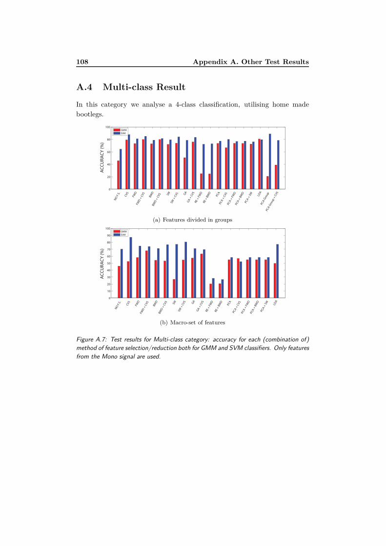
108 Appendix A. Other Test Results
A.4 Multi-class Result
In this category we analyse a 4-class classification, utilising home made
bootlegs.
0
20
40
60
80
100
AC
CU
RA
CY
(%
)
NO
F.S
.
CV
S
FWD
FWD
+ C
VS
BW
DB
WD
+ C
VS SW
SW +
CV
S GA
GA
+ C
VS
RE
+ F
WD
RE
+ B
WD
PCA
PCA
+ C
VS
PCA
+ F
WD
PCA
+ B
WD
PCA
+ S
W
LDA
PCA
Gro
up
PCA
Gro
up
+ C
VS
GMM
SVM
(a) Features divided in groups
0
10
20
30
40
50
60
70
80
90
100
AC
CU
RA
CY
(%
)
NO
F.S
.
CV
S
FWD
FWD
+ C
VS
BW
DB
WD
+ C
VS
SW
SW +
CV
S
GA
GA
+ C
VS
RE
+ F
WD
RE
+ B
WD
PCA
PCA
+ C
VS
PCA
+ F
WD
PCA
+ B
WD
PCA
+ S
W
LDA
GMM
SVM
(b) Macro-set of features
Figure A.7: Test results for Multi-class category: accuracy for each (combination of)
method of feature selection/reduction both for GMM and SVM classifiers. Only features
from the Mono signal are used.

A.4. Multi-class Result 109
0
20
40
60
80
100
AC
CU
RA
CY
(%
)
NO
F.S
.
CV
S
FWD
FWD
+ C
VS
BW
DB
WD
+ C
VS
SWSW
+ C
VS
GA
GA
+ C
VS
RE
+ F
WD
RE
+ B
WD
PCA
PCA
+ C
VS
PCA
+ F
WD
PCA
+ B
WD
PCA
+ S
W
LDA
PCA
Gro
up
PCA
Gro
up
+ C
VS
GMM
SVM
(a) Features divided in groups
0
10
20
30
40
50
60
70
80
90
100
AC
CU
RA
CY
(%
)
NO
F.S
.
CV
S
FWD
FWD
+ C
VS
BW
DB
WD
+ C
VS
SW
SW +
CV
S
GA
GA
+ C
VS
RE
+ F
WD
RE
+ B
WD
PCA
PCA
+ C
VS
PCA
+ F
WD
PCA
+ B
WD
PCA
+ S
W
LDA
GMM
SVM
(b) Macro-set of features
Figure A.8: Test results for Multi-class category: accuracy for each (combination of)
method of feature selection/reduction both for GMM and SVM classifiers. Features
both from Band and Mono signal are used.


![ComputationalVaccinology:AnImportantStrategyto … · 2011. 6. 1. · DNA vaccine ND IgG, IgG1 > IgG2a ND 38.1% ND [33] Sm 25 Peptide vaccine ND IgG No significative difference](https://static.fdocuments.in/doc/165x107/609fc21e5f4e7561c46ccc5b/computationalvaccinologyanimportantstrategyto-2011-6-1-dna-vaccine-nd-igg.jpg)


