Political Risk and Firm Default Probability

­Exploring Export Credits to High­Risk Countries

August, 2006

Preliminary version, comments welcome

Annika SandströmDepartment of Finance and Statistics

Swedish School of Economics and Business Administration

P.O.Box 479, FIN­00101 Helsinki,  FINLANDe­mail: annika.sandstrom@hanken.fi

Political Risk and Firm Default Probability

­

Exploring Export Credits to High­Risk Countries

Abstract

Despite the increased presence and importance of political risk and export credit financing in the

world economy, these topics have not been well covered in the empirical credit risk literature. In

this  article, we  model default  probabilities  for private  firms  from selected high­risk  countries,

and condition these on a vector of country specific political risk variables, indicators of the level

of  democracy,  legal  environments  and  the  quality  of  credit  information,  in  addition  to  the

traditional  firm  specific  financial  variables  usually  employed.  The  study  is  an  empirical

application to a unique dataset on export credit facilities, not studied previously in a credit risk

framework.  The  preliminary  results  from  Argentina,  Indonesia,  Nigeria,  Poland  and  Saudi

Arabia  indicate  that  information on socioeconomic conditions, military  in politics  and external

conflict in a country constitute significant predictors for firm default, that may not otherwise be

detected with scarcely available, or unreliable accounting information.

Key Words:   Probability of Default; Company Failure Risk; Export Credits; Political Risk

1

1.   Introduction

Analysis  of  financial  statements  is  the  starting  point  in  any  classification  of  companies  into

healthy  and  financially  distressed  (or  bankrupt)  firms.  Among  the  first  known  attempts  to

distinguish companies based on their accounting is Fitzpatrick (1932), who compared financial

ratios  between  successful  industrial  enterprises  from  those  that  failed,  and  found  that  the

probability of default was  related  to  the  individual  characteristics of  firms. Since  then,  a  large

number of empirical studies has been published and well known applications of credit scoring,

e.g.  the  Altman’s  Z­Score  model  (Altman,  1968)  and  the  Moody’s  KMV  EDF RiskCalc

Model, are widely used in the industry. These accounting­based models are usually applied when

no  publicly  traded  securities  are  available  or  when  secondary  market  prices  are  unreliable.

Meanwhile,  some of  the caveats of  the  accounting­based models  is  that  they  rely  on  financial

statements that capture the past performance of  the firm  rather than its future performance. As

noted by Hol et al. (2002),  it still seems that  the extensive research effort on bankruptcy­, and

default prediction has failed to produce an agreement on which variables are good predictors and

why.  This  may  be  partly  attributed  to  the  fact  that  the  studies  refer  to different  time  periods,

countries and industries. Most studies are also claimed to lack a theoretical framework to guide

the  empirical  research  effort1.    Traditionally,  default  probability  is  estimated  from  failed  and

non­failed firms, given historical data using annual  financial statements.    In  this paper, we ask

whether  there  could  be  other  important  factors  to  consider,  in  order  to  improve  model

performance,  especially  in  situations  when  the  financial  information  is  scarcely  available  or

unreliable, as might be the case in developing countries.

1 Hol et al. (2002) have recently suggested a capital structure based default theory.

2

While  the  financial  figures  of  a  company  are  the  basis  for  evaluating  its  credit  profile,  non­

financial  and  environmental  characteristics  seem  necessary  to  complete  the  picture.  The  new

approach in this paper is  to discuss linkages between firm default probability and  the political­

and legal risk environments that prevail in the country where the borrowing company operates.

To what  extent do political  events or unstable  legal  environments constitute a  risk  for  foreign

lenders, that might not otherwise be reflected in the financial figures of the borrowing company?

The main objective of  this study  is  to  assess whether political­  and commercial  factors can be

distinguished in the credit risk assessment process.

A novel feature of the present study is also the use of export credit guaranteed debt contracts in

the attempt to model default probabilities from realized payment interruptions2. We empirically

explore the relationships between default probabilities and political risk for a group of firms from

selected high­risk countries, including Argentina,  Indonesia, Nigeria, Poland and Saudi Arabia.

In  this  version of  the paper,  these  countries  are selected  to  represent examples of most  active

recipients of world­wide export credits among developing countries, and reflect also the largest

export streams from Finland to developing countries in the last two decades.

The remainder of this paper is organized as follows. Section 2 provides a brief literature review

on default probability estimation. In section 3, we discuss the question of the impact of political

risk  on  credit  defaults  and  formulate  our  main  research  hypothesis.  Section  4  presents  our

research design and data in more detail. In section 5, we present our results with a short analysis

of our target countries. Section 6 concludes with suggestions for further research.

2 This type of data has not been previously addressed in similar credit risk­ or default probability studies, due to a general secrecysurrounding  Export  Credit  Agencies  and  consequently,  the  unavailability  of  data.  For  the  purposes  of  this  research  project,initiated in co­operation with the Finnish Export Credit Agency, Finnvera plc, we have the unique opportunity to explore archivesof historical credit­ and political risk data from various countries.

3

2.    Default probability estimation

There are two schools of  thought  in  the use of  statistical methods  to predict firm default. One

holds that default is modeled using accounting data, whereas the other recommends using market

information.  Accordingly,  the  existing  models  are  usually  classified  into  the  market­based

models, which rely on security prices, and the so called fundamentals­based models, which can

further be divided in models that rely on accounting, systematic market and economic factors, or

rating information. In this study, for brevity reasons and in order to follow our research set­up for

private firms, we will focus mainly on the accounting­based models4.

Fundamentals­based estimation with accounting info

The  literature  on  credit  scoring  is  based  on  the  original  work  of  Beaver  (1966)  and  Altman

(1968). Being a classic among the early studies, Beaver (1966) conducted a comprehensive study

using a variety of  financial  ratios and concluded that  the cash flow to debt ratio was the single

best predictor of firm default. Beaver’s univariate approach of discriminant analysis led the way

to  a multivariate  analysis  by  Altman  (1968) who adopted  a multivariate  discriminant  analysis

(MDA) framework in his effort to find a bankruptcy prediction model. This became the popular

Z­score  model,  where  the  financial  ratios  used  are:  1)  working  capital  over  total  assets;  2)

retained earnings over total assets; 3) earnings before interest and taxation over  total assets; 4)

market value of equity over book value of liabilities; and 5) sales over total assets. In Altman’s

study,  the  Z­Score  correctly  classified  94%  of  the  bankrupt  companies  and  97%  of  the  non­

bankrupt  companies  one  year  prior  to  bankruptcy.  Later,  Altman  has  revised  the  model  for

private firms by substituting book value for market value in the calculation of the ratio of market

4 For a good review of the market­based models, see e.g. Chan­Lau (2006)

4

value  of  equities  to  the  book  value  of  liabilities5.  The  popularity  of  the  Altman  Z­score  is

explained by its parsimony and ease of interpretation. Some of its shortcomings are discussed in

Engelmann et al (2003).

Explanatory variables and statistical techniques

A large number of financial ratios can be used as explanatory variables in the accounting based

models.  Typically,  the  greatest  variations  in  the  probabilities  of  default  come  from  ratios

capturing firms’ profitability, growth opportunities, level of indebtness, and liquidity. To obtain a

parsimonious  model, some  selection  criteria  are needed,  and  the variables  selected  are usually

those with the higher discriminating power for explaining the default frequency after performing

univariate  analysis.  However,  these  steps  can  only  be  taken  once  a  robust  database  has  been

compiled. There is usually also the risk of “over­fitting”, that is, the model functions only on the

sample data but fails to engage with real­world data that it has not “seen” before.

Once variables have been selected, a variety of statistical techniques have been used to assess the

default  probability  of  a  firm,  including  econometric  models,  linear  discriminant  analysis,  k­

nearest neighbor classifier, neural networks, and support vector machine classifier among others

(Chan­Lau,  2006).  For  obvious  problems  with  the  assumptions  of  the  initially  employed

discriminant  analysis,  discrete  dependent  variable  econometric  models  (i.e.  logit  or  probit

models),  have become  more popular  tools  for  credit  scoring.  Ohlson  (1980)  and  Platt & Platt

(1990)  present  some  of  the  early  studies  using  the  logit.  A  more  recent  example  is  Laitinen

(1999),  who  used  automatic  selection  procedures  to  select  the  set  of  variables  to  be  used  in

logistic and linear models, which were then thoroughly tested out­of­sample.

5  A summary of the methodologies is given in Chuvakhin & Gertmenian (2003)

5

3.   Political risk and credit

Political  risk may be defined as "the probability of  the occurrence of  some political event  that

will change the prospects for the profitability of a given investment”. This definition, originally

given  by  Haendel  (1979),  appears  often  in  studies  of  political  risk  due  to  its  simplicity  and

flexibility against the interest and need of the definer (e.g. a corporate, a private insurance firm,

an export credit  agency, a bank or  a multinational organization).  In  the credit  risk framework,

political risk may be defined as “the possibility of delayed, reduced, or non­payment of interest

and  principal  where  the  outcome  is  attributable  to  the  country  of  the  borrower”  (Caouette,

Altman and Narayanan, 1998).

There  has  been  a  growing  interest  in  the  academic  literature  on  the  link  between  political

institutions and political risks facing multinational corporations. A large part of this research  is

devoted  on  domestic  institutions  and  FDI  inflows  (see  e.g.  Henisz  2002,  and  Jensen  2006).

Meanwhile, only few authors have investigated the relationship between political risk and credit,

and  the  focus has been mainly on sovereign borrowing (see e.g. Citron and Nickelsburg 1987,

Balkan  1992,  Edwards  1986,  Brewer  and  Rivoli  1989  and  Peter  2000)  and  the  relationship

between democratic  institutions and borrowing (see e.g. Schultz and Weingast 2003 and Saiegh

2005).   To  the best of our knowledge,  there are no prior studies using political  risk  factors  to

study corporate credit defaults.

Hypothesis development

The  overall  hypothesis  in  the  present  study  is  that  outcomes  from  lending  decisions  to

importing/borrowing companies are uncertain not only because of the company as an individual

obligor, but also due to surrounding political­ and legal risk factors, that may have nothing to do

with the firm itself. We ask to what extent comprehensive measures of political  risk would be

6

useful in the assessment of default probabilities at the transaction level.

We conjecture that the political risk in a country affects the credit risk of  firms operating in the

country  through  sub­categories  of  political  risk,  identified  as  1) risk  of  expropriation or

confiscation  (e.g.  of  the  exported  merchandise  by  a  foreign  government);  2) risk  of  currency

convertibility  and  transferability  (i.e.  the  customer  in  the  foreign  country  is  unable  to  obtain

foreign  exchange  in  order  to  pay  or  is  unable  to  send  payments  out  of  the  country  due  to

governmental restrictions or foreign exchange transfers); and 3) political violence (war, sabotage

or terrorism). All these situations involve specific risks that might cause a buying firm that would

otherwise be willing to pay the creditor to be unable to do so. In addition, there might be other

unanticipated changes in regulations, corruption or failure by the government to implement tariff

adjustments because of political considerations. Further, quasi­commercial risks may arise when

the project or business of the company is facing state­owed suppliers or customers, whose ability

or willingness to fulfill their contractual obligations towards the project might be questionable.

Ultimately, political  risk  relates  to  the preferences  of political  leaders,  parties,  and  actions,  as

well as their capacity to execute their stated policies when confronted with internal and external

challenges.  Changes  in  the  regulatory  environment,  attitudes  towards  corporate  governance,

reaction  to  international  competition,  labour  laws,  witholding  and  other  taxes  are  concerns,

which may all affect the firm in an extent leading to non­payment of its obligations. The causes

for  the above conditions may be  influenced by hard  to discern shifts  in  the political  landscape

(Bremmer et al. 2006), so the big challenge in any studies on political risk is how to measure it.

7

Measuring Political­ and Legal Risk

In  this  study, we analyze  political­  and  legal  risk  through  selected  indicators  employed  in  the

International  Country  Risk  Guide  (ICRG),  Polity  IV  Project  and  the  World  Bank’s  “Doing

Business”  database.  These  ratings  are  all  illustrative  of  the  above  stated  conditions  from  a

project­ and company perspective.

The  ICRG  system  by  the  PRS  Group  is  a  numerical  rating  system  that  scores  a  number  of

components  for political, economic and  financial  risk  to determine a  rating for each category6.

We use the ICRG Political Risk Rating and its sub­components, which aim to provide a means of

assessing the political stability of countries on a comparable basis. ICRG assigns risk points to a

pre­set of group of  factors,  termed political  risk  components. The  range  of  points  that  can be

assigned  to  each  component  varies  between  zero  and  a  fixed  weight,  that  the  particular

component  is  given  in  the  overall  political  risk  assessment.  The  lower  the  risk  point  total

indicates  for  higher  political  risk,  so  we  expect  an  inverse  relationship  with  firm  default

probabilities.

Appendix I lists the political risk components for the ICRG Political Risk Rating (icrg). Among

the  components,  for  example, Democratic  accountability  (Component  K)  is  an  indicator  of

whether  a  government  will  take  precipitous  actions  such  as  expropriation. Law  and  Order

(Component I) is seen as an indicator of the stability and transparency of the legal system and an

indication of whether contracts might be abrogated. Ethnic tensions (Component J) are often a

preliminary condition to strife that leads to political violence against investors and creditors, or

on their property.

6 These three ratings are used to determine an overall composite rating, a number from 0 to 100 (zero being high risk, 100 beingthe lowest risk).

8

In addition to the ICRG risk components, we will also test for other measures of the legal­ and

political system in a country (also listed in Appendix 1). We describe the quality of a country’s

political  institutions  in  terms of  the exposure  to democracy; using  the "Polity  Index" from  the

Polity  IV  dataset.  This  index  measures  the  degree  to  which  a  nation  is  either  autocratic  or

democratic on a scale from ­10 (strongly autocratic) to +10 (strongly democratic). According to

the  “democratic  advantage”  argument,  democracies  pay  lower  interest  rates  for  the  sovereign

debt than authoritarian regimes because they are better able to make credible commitments (see

e.g. Schultz and Weingast 1996, 1998). We test whether this argument is reflected also on firm

level  and  expect  a  negative  relationship  between  default  probabilities  and  the  level  of  host

country democracy.

We  define  political  stability  also  in  terms  of  the  frequency  of  regime  change.  This  is

approximated in  the “Polity IV Regime Durability Variable” (durable),  that measures the years

since the most recent regime change or the end of a transition period defined by the lack of stable

political institutions. We expect a negative relationship with firm default probabilities, that is, the

longer the time since last regime change, the lower is the firm probability of default.

Finally,  we  ask  how  legal­  and  financial  rights  of  the  creditor  and  debtor  affect  default

probabilities?  On  the  one  hand,  legal  costs  may  prevent  the  borrower  to  incur  a  “strategic

default”,  where  the  firm  fails  to pay  the  amount  stipulated  in  the debt  contract  even  though  it

possesses  resources  to  do  so.  On  the  other,  with  costly  liquidation,  creditors  may  prefer  to

forgive part of debt, which may result in equityholders’ incentives to default opportunistically7.

7   See e.g. Davydenko and Strebulaev (2003).9   This includes manually kept records from the 1980s as well as electronic registers from the later decade.

9

To capture  the effects of  legal  risk,  we  include  two additional  indices  from  the World Bank’s

Doing  Business  database, that  measure  credit  information  registries  and  the  effectiveness  of

collateral and bankruptcy  laws in facilitating lending. The legal rights index (legal)  reflects  the

legal  rights  of  borrowers  and  lenders,  by  measuring  the  degree  to  which  collateral  and

bankruptcy  laws  facilitate  lending.  The  index  includes  3  aspects  related  to  legal  rights  in

bankruptcy and 7 aspects found in collateral law. It has a scale from 0 to 10, with higher scores

indicating that collateral and bankruptcy laws are better designed to expand access to credit. The

credit information index (credit) measures rules affecting the scope, accessibility and quality of

credit information available through either public or private bureaus. The index ranges from 0 to

6, featuring the credit information system. Higher values indicate that more credit information is

available  from  either  a  public  registry  or  a  private  bureau  to  facilitate  lending  decisions.  A

negative  sign  is  expected  for  these  variables,  that  is,  better  laws  in  place  or  more  credit

information available lowers the firm probability of default.

4. Research Design

We model the default probability for a set of borrowing firms, using a dynamic binary estimation

method where the dependent variable is 1 if the firm defaults in a specific year and 0 otherwise.

The estimated default probabilities are conditioned over a vector of lagged explanatory variables

including  firm­specific  financial  ratios  and country­specific political­  and  legal  risk  indicators.

We use export  credit  guaranteed debt contracts, and  to  the greatest extent possible, we aim to

picture  a  realistic  decision  making  process  at  the  time  when  the  lending  decision  was  made.

What comes  to  lending  to high­risk  countries,  there  is usually  a  special  concern  regarding  the

availability and reliability of the financial information.

10

Data Considerations

The main data for our research project is obtained from the official Export Credit Agency (ECA)

of Finland, Finnvera plc,  that consists of  trade credit contracts  (i.e. commercial  loans between

Finnish exporters  and  foreign buying companies),  between years  1980­2005.   These  loans  are

granted  by  banks  or  other  financial  institutions  and  guaranteed  by Finnvera  plc against

commercial  and  political  risks.  Detailed  credit  information  underlying  each  guarantee  is

collected  by  combining  data  from  comprehensive  records  of Finnvera  plc9.  This  information

includes dates of initiation and the end of the contract; identification number for each guarantee,

information on the parties involved, default date and  indemnifications (if any), contract values,

currencies, trade items etc. During the 25­year study period, some 30 000 contracts were in force

between Finland and importing companies from over 132 different countries around the world.

Country­ and Sample Selection

The selected data for this study consists of export credit guaranteed debt contracts between  the

Finnvera plc and companies from Argentina, Indonesia, Nigeria, Poland and Saudi Arabia10. The

selection of  these  countries  for  this  version of  the  paper  is based on  choosing  the  most  active

‘high­risk’ export countries of Finland during the last decades, representing five different world

regions. Also on a  larger  scale,  these countries  represent  type examples of countries  that have

received  the  majority  of  world  export  credit.  For  example,  in  1996,  Indonesia,  Nigeria  and

Poland were among the top ten countries, that together accounted for 30 percent of the industrial

country ECAs’ contribution (see Table 1). Argentina, is our example country from the financial

crisis affected Latin American region and Saudi Arabia represents an oil­dependent, arab nation.

At the policy level,  there are of course no obvious reasons to compare these countries as such.

10 In our further research agenda, we plan to append our country selection.

11

Instead, we consider them as type examples of countries facing various economic, commercial

and political risks, where an increasing number of western businesses may still find it desirable

to export and invest in.

We employ the following criteria in our further sample selection;

§ Only firms that are outside governmental control are included in the sample. Thus, credit

counterparts that are public bodies or state­owned enterprises, are excluded11.

§ All industries, except financial sector firms, are included. As common in similar studies,

we exclude banks and financial firms due to the specificity of their financial statements.

§ All different types of guarantee contracts issued by Finnvera are included in the sample.

The most common forms of export credit are buyer credit­, credit risk­ and letter of credit

guarantees, which are also the most common forms of contracts in our sample12.

§ We include contracts  that have been effective during some time period between 1980 ­

2005. Thus, some guarantees in the sample have been initiated before 1980 but are still in

force during our study period.

§ Due to limitations in the oldest data and the problem of changes in accounting methods,

we collect data on firm financial variables for firms/guarantees effective after year 1989.

§ We define default as any payment interruption by the debtor company, that deviates from

the scheduled payments stipulated in the guarantee contract.

With these criteria and definitions, our sample consists of 1003 guarantees of which 128 (12.8%)

have  experienced  a  default.  Summary  statistics  of  the  credit  data  employed  are  presented  in

Figures 1­2 and Tables 2­4.

11 Due to their specific relation to political risk, these are treated separately in an earlier article (Sandström, 2005).

12

For our modeling purposes, we measure our data  in  firm years,  taking  into account  the yearly

stock of undefaulted effective guarantees  and  the  stock of non­expired  guarantees  in  a default

state.  For  each  guarantee,  we  know  whether  there  has  been  an  application  for  loss  on  the

underlying claim as well as the indemnifications by Finnvera. We don’t know the exact dates for

the  loss claim decision, but have the dates  for  the corresponding  first and  last  indemnification

payments. Accordingly, we consider the loan in a default state between these dates and analyze

the data  in  yearly  intervals. According  to  Basel  II, we  specify  the  time horizon  for  the  future

probability of default  as one year which is consistent with  the use  in  the banking practice and

prevalent in credit risk models.

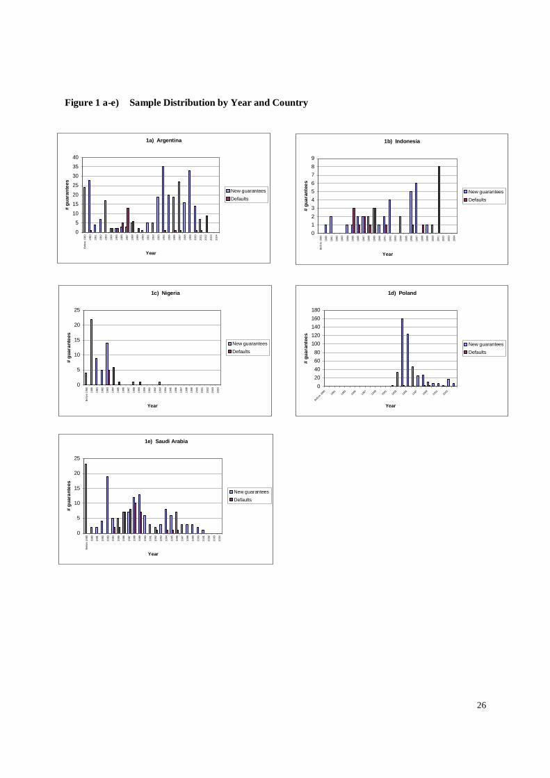
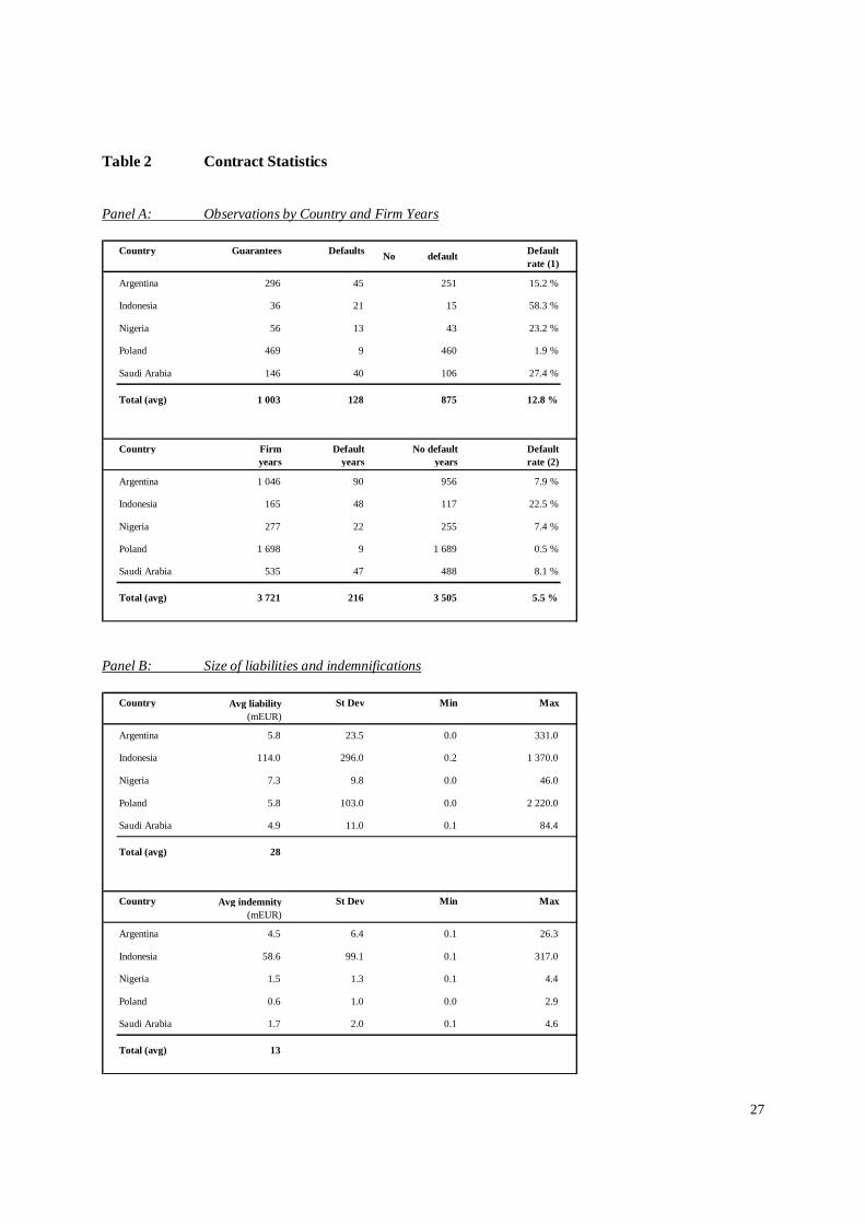
Figures  1a­e)  illustrate  the  yearly  distribution  of  new  issued  guarantees  and  the  number  of

defaults by  sample countries. Summary  statistics  on  credit contracts  and  firm­years  by default

status  and  by  country  are  summarized  in  Table  2  (Panel  A).  Average  liabilities  and

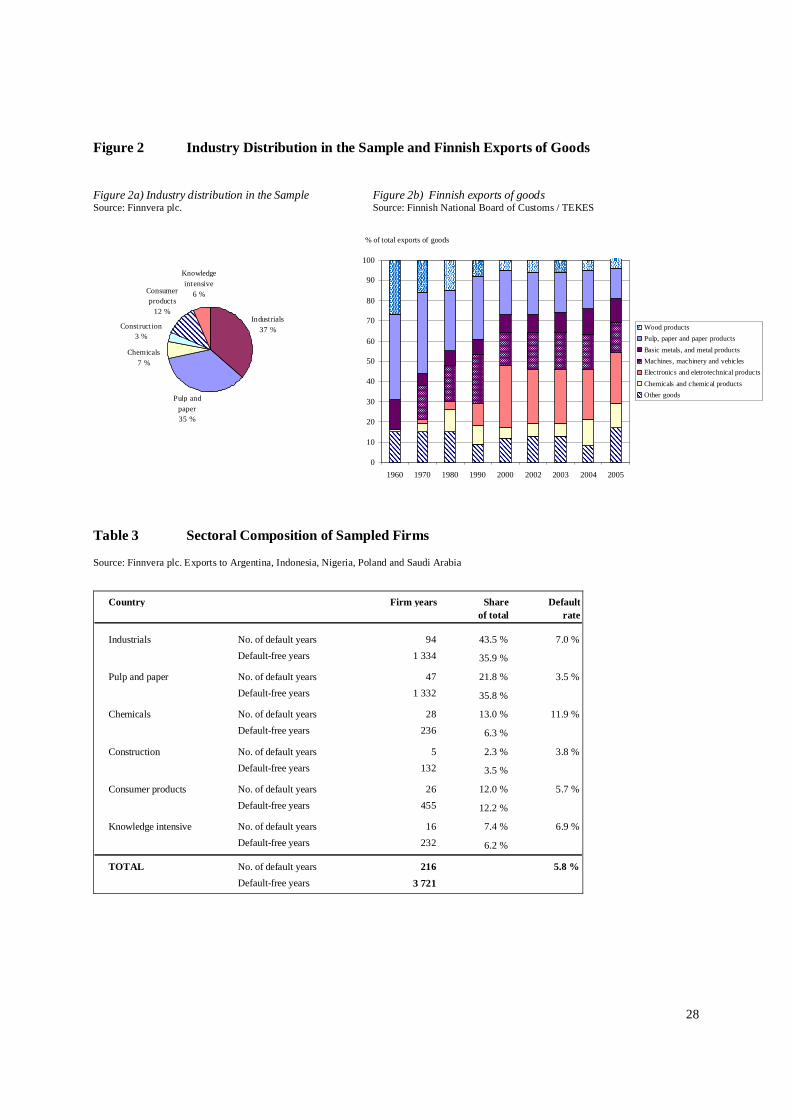
indemnifications by country are  summarized  in Table 2  (Panel B). Figures 2a  and 2b compare

the industry distribution in our sample with the total Finnish Exports given by industry. Pulp and

paper have  traditionally  accounted  for most of  the Finnish exports. However,  in  the 1980s,  its

majority share of exports started to fall as a result of the rapid growth in the industrial sector (e.g.

basic metals and metalworking; transport equipment; and electrical equipment). Shipbuilding in

particular, has  led the development of heavy  industry,  and  is  the most  important branch of  the

transport sector13. The woodworking industry fostered also the industrials sector through its need

of papermaking equipment (e.g. mechanical and machine building) as well as the chemical sector

(bleaching,  water  purification,  packaging  materials  etc.).  As  shown  in  Table  3  our  sample  is

fairly  evenly  split  up  in  the  industry  groups,  both  in  number  of  guarantees  and  in  defaults.

12 A special type, an Investment Guarantee emerges a few times in our sample. The difference is that it is bigger in size, and theforms of investment which can be covered under this include equity investments, shareholder loans and guarantees granted by ashareholder. For our purposes, the nature of the guarantee does not affect model estimation.

13

Firm Financial Variables

We  choose  accounting  variables  based  on  how  the  decision  process  was  initially  undertaken,

considering the available information when the credit was granted. Following previous literature,

we select available ratios that measure different dimensions of companies’ healthiness, including

size, age, turnover, profitability, leverage liquidity and solidity.  The definitions of the selected

financial ratios are provided in Appendix 2.

In order to collect the available financial figures, a sample of 108 annual, end­of­year corporate

financial statement summaries are extracted from Finnvera's credit report database. These yearly

statements belong to 402 unique guarantees, from 1989 to 2005, of which 23 (5.7%) have had at

least  one  payment  interruption  or  default  in  a  given  year.  The  financial  accounts  have  been

originally  obtained  from  reliable  sources  including  Suomen  Asiakastieto  Oy,  the  leading

business  and  credit  information  company  in  Finland,  whose  data  sources  comprise  the  data

subjects, the authorities, and reliable partners14. A smaller part of the credit reports were obtained

from Dun & Bradstreet Credit Bureau and some complements were made directly from available

company  financial  reports. Summary statistics of  the firm financial  ratios are given  in Table 4,

where  Panel  A  presents  the  whole  sample  and  Panel  B  the  compares  defaulting  and  non­

defaulting firms. Summary statistics for political­ and legal risk indices (introduced in Section 3)

are presented in Table 5. Table 6 presents the correlations between firm financial­ (Panel A) and

political­ (Panel B) and the combined group (Panel C) of explanatory variables. The correlations

are generally very low (in most cases under ±0.2 ), except for icrg and its components, which are

naturally not tested jointly.

13 The biggest guarantee offers by Finnvera are applied to telecommunications and to shipping and shipbuilding.

14

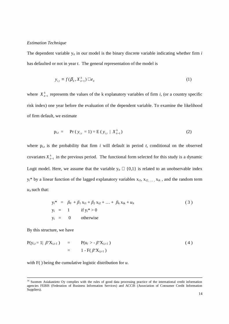
Estimation Technique

The dependent variable yit in our model is the binary discrete variable indicating whether firm i

has defaulted or not in year t.  The general representation of the model is

itkitkti eXfy += − ),( 1, β (1)

where kitX 1−  represents the values of the k explanatory variables of firm i, (or a country specific

risk index) one year before the evaluation of the dependent variable. To examine the likelihood

of firm default, we estimate

pi,t  =    Pr ( tiy ,  = 1) = E ( tiy ,  | kitX 1− ) (2)

where  pi,t  is  the  probability  that  firm i will  default  in  period t,  conditional  on  the  observed

covariates kitX 1−  in the previous period.  The functional form selected for this study is a dynamic

Logit model. Here, we assume that the variable yit ∈ {0,1} is related to an unobservable  index

yi* by a linear function of the lagged explanatory variables xi1, xi2, … . , xik , and the random term

uit such that:

yi*   = 0  + 1 xi1 + 2 xi2 + …  + k xik + uit ( 3 )

yi   =  1 if yi* > 0

yi   =   0 otherwise

By this structure, we have

P(yi,t = 1| ‘Xi,t­1 )  = P(ui  > ­ ‘Xi,t­1 ) ( 4 )

  = 1 ­ F( ‘Xi,t­1 )

with F( ) being the cumulative logistic distribution for u.

14  Suomen  Asiakastieto  Oy  complies  with  the  rules  of  good  data  processing  practice  of  the  international  credit  informationagencies  FEBIS  (Federation  of  Business  Information  Services)  and  ACCIS  (Association  of  Consumer  Credit  InformationSuppliers).

15

Our methodology is an attempt to respond to the concerns of a single­period logit approach15,  as

suggested in Shumway (2001) and Beck et al  (1998), and will be further  refined in our  further

research work (e.g. to account for intertemporal correlation). Beck et al. (1998) demonstrate that

the use of ordinary single­period logit or probit on binary time­series/cross­sectional data (such

as  default  study  data)  can  result  in biased  and  inconsistent  coefficients,  as  well  as  inflated  t­

statistics.  A  logistic  discrete  hazard  model  overcomes  these  methodological  problems  by

formally  incorporating the dynamic nature of corporate default (see e.g. Hillegeist et al. 2004).

A  logistic  discrete  hazard  model,  which  is  a  discrete  approximation  to  the  Cox  proportional

hazard model has the following form:

X ti,+=−

)(1

log,

, tp

p

ti

ti α ,   or (4)

X

X

ti

ti

,

,

)(

)(

, 1 +

+

+= t

t

ti eep α

α

(5)

where X ti,   represents  the  independent variables observable at  the end of year t and )(tα   is a

time­varying  covariate  that  captures  the  underlying  “baseline”  hazard  rate.  This  maximum

likelihood estimator  differs  from  ordinary  logit  by  1)  the  subscript t ,  that  reflects  the use of

multiple years of data for the same firm, and 2) discrete hazard model that includes the baseline

hazard  rate )(tα . This allows a  firm’s probability of default  (and  the associated covariates)  to

change  over  time.  In  this  version  of  the  paper,  we  run  the  multiyear  logit  regressions  by

assuming that the baseline hazard is constant.

15  Including  1)  a  sample  selection  bias  from using  only  one,  non­randomly  selected  observation  per defaulting  firm,  and  2)  afailure to model time­varying changes in the underlying or baseline risk of default that induces cross­sectional dependence in thedata.

16

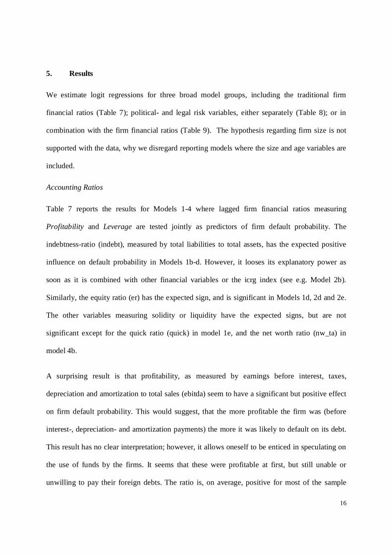
5.   Results

We  estimate  logit  regressions  for  three  broad  model  groups,  including  the  traditional  firm

financial  ratios  (Table 7);  political­  and  legal  risk  variables,  either  separately  (Table  8);  or  in

combination with the firm financial ratios (Table 9).   The hypothesis  regarding firm size  is not

supported with the data, why we disregard reporting models where the size and age variables are

included.

Accounting Ratios

Table  7  reports  the  results  for  Models  1­4  where  lagged  firm  financial  ratios  measuring

Profitability and Leverage  are  tested  jointly  as  predictors  of  firm  default  probability.  The

indebtness­ratio  (indebt),  measured by  total  liabilities  to  total  assets, has  the expected positive

influence  on  default  probability  in  Models  1b­d.  However,  it  looses  its  explanatory  power  as

soon  as  it  is  combined  with  other  financial  variables  or  the  icrg  index  (see  e.g.  Model  2b).

Similarly, the equity ratio (er) has the expected sign, and is significant in Models 1d, 2d and 2e.

The  other  variables  measuring  solidity  or  liquidity  have  the  expected  signs,  but  are  not

significant  except  for  the  quick  ratio  (quick)  in model 1e,  and  the  net  worth  ratio  (nw_ta)  in

model 4b.

A  surprising  result  is  that  profitability,  as  measured  by  earnings  before  interest,  taxes,

depreciation and amortization to total sales (ebitda) seem to have a significant but positive effect

on  firm default probability.  This  would  suggest,  that  the more profitable  the  firm  was  (before

interest­, depreciation­ and amortization payments) the more it was likely to default on its debt.

This result has no clear interpretation; however, it allows oneself to be enticed in speculating on

the  use  of  funds  by  the  firms.  It  seems  that  these  were  profitable  at  first,  but  still  unable  or

unwilling  to pay  their  foreign debts. The  ratio  is,  on  average, positive  for  most of  the  sample

17

firms with a mean value around 10%  for  the non­defaulting firms,  and 20% for  the defaulting

firms  (see Table 4). This  result may, of  course, be caused by  too  few observations  (the ebitda

figure  is  available  for  only  9 defaulting  firms).  Firm net profit  as  a  percentage of  total  assets

(profit_ta) has the expected negative sign and is significant in Models 3a, 3b, 4a, and 4b. While

the significance of some of  the  individual coefficients  in  the model are  indicative,  they do not

provide evidence concerning the collective group significance of accounting information.

We  continue  our  analysis  in  Table  7  by  combining  firm  financial  ratios  with  the  ICRG

Composite Political Risk Index (icrg) in Models 2 and 4. In all except one of the Models  (4e),

this ratio gives the expected sign and is highly significant (at 1% level in Models 2a­d, 4a and at

5% level  in Models 4b­4c). Looking at the overall p­values for  the models in Table 7, one can

conclude that they are statistically significant.

Political and Legal Risk

We next  focus on political­ and legal risk indicators as predictors of  firm default probabilities.

The  general  principle,  when  interpreting  these  results  is  that  a  negative  coefficient  for  any

political­  or  legal  variable,  indicates  that  an  increase  in  the  ratio  (less  risk)  reduces  the

probability of  firm default.  In various  logit  regressions16, most of  the ICRG components show

the expected sign and are significant when tested separately. Combined in with each other,  the

significance usually diminishes, except for the components measuring Socioeconomic Conditions

(socec),  External  Conflict (extcon) and Military  in  Politics (mil). Socioeconomic  pressures  at

work  in  a  society  may  constrain  government  action  or  fuel  social  dissatisfaction,  leading  to

further instabilities. The risk rating is the sum of three subcomponents, including unemployment,

consumer confidence and poverty.  It is conceivable that these malfunctions in society may well

16 Not reported here for brevity reasons; details on these are available from the author upon request.

18

lead also to firm deteoriation, and subsequently to its default. The External Conflict measure is

an assessment both of  the risk  to  the  incumbent government from foreign action, ranging from

non­violent  external  pressure  (diplomatic  pressures,  withholding  of  aid,  trade  restrictions,

territorial disputes, sanctions,  etc)  to violent external pressure  (cross­border conflicts  to all­out

war). One interpretation for the obtained result is that different forms of bilateral punishments do

not seem to act as enforcement mechanisms for debt repayments, but rather the opposite (see e.g.

Rose,  2002).  However,  external  conflicts  may  also  affect  businesses  adversely  in other  ways,

ranging from restrictions on operations,  to  trade and  investment sanctions,  to distortions  in  the

allocation  of  economic  resources.  Thus,  any  interpretation  of  the  external  conflict­variable

should be adjusted to the country and circumstances in question. Generally, these results would

suggest  that  the  more  external  pressure  a  country  has,  the  more  the  firms  operating  in  that

country are likely to default on their foreign obligations.

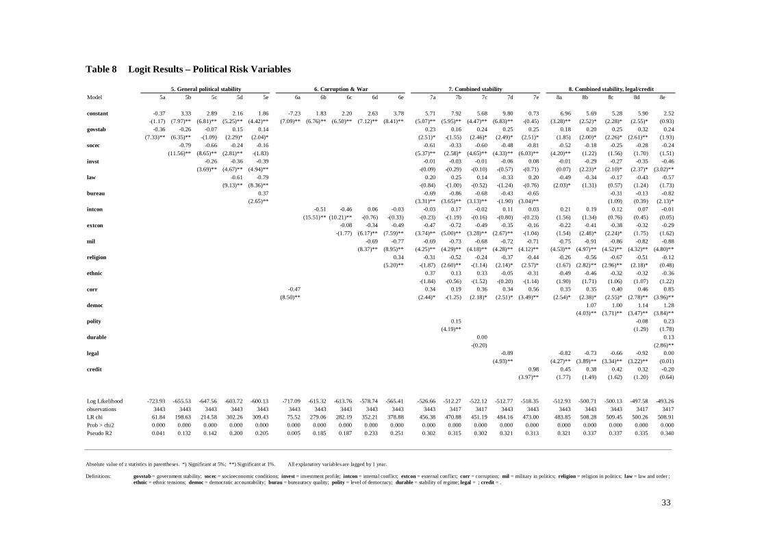
It  would  be  misleading  to  claim  that  only  one  political  risk  rating  would  serve  as  a  single

predictor variable for firm default. Thus, we present the results in groups measuring 1. General

Political  Stability (including  government  stability,  socioeconomic  conditions,  investment

climate,  law  and  order  and  bureaucratic  accountability);  2. Corruption&War  (including

components  of  corruption,  internal­  and  external  conflict,  military­  and  religion  in  politics  as

well as ethnic tensions); and 3. Combined stability (with all included). Table 8 report the various

results for these groupings. Again, the component measuring Socioeconomic Conditions, remains

a significant predictor of firm default probability (7a­e, 8a). Similarly, in models 6d­e, 7a­d, 8b­c

the External Conflict component is again negative and significant. Regarding the other political­

and legal risk indices, no clear­cut patterns may be observed from this data17.

17 The measure of corruption, is significant when measured alone. However, when combined with other components, it changessign  and becomes  insignificant.  The  Legal  rights  Index  is  significant only  in  models  7d and 8a­e.  The  Creditor Rights  Indexremains insignificant with a opposite sign to the hypothesized.

19

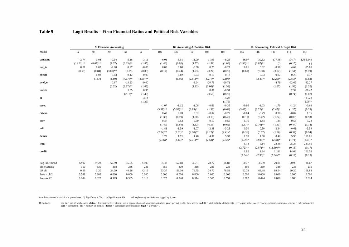
Combined Accounting Information, Political and Legal Risk

Finally,  table  9  reports  the  results  for  the  models,  where  financial  ratios  are  combined  with

selected political­ and legal indicators. Again, we find interesting results for the ebitda­measure,

which  shows  positive  and  significant  coefficients  (see  e.g.  models  9d­e,  10d­e  and  11b­d).

Meanwhile, the indebtness measure is significant only in one of the models (9d). On the political

risk side,  the Socioeconomic conditions component show again the same significant patterns as

before.  Also  the Military  in  Politics component  (mil)  is  significant  and  negative  (e.g.  models

10a­e).  The  military’s  involvement  in  politics,  even  at  a  peripheral  level,  can  be  seen  as  a

diminution  of  democratic  accountability,  and  an  indication  that  the  government  is  unable  to

function  effectively.  The  signs  for  the other political­  and  legal  indices,  when combined  with

firm  financial  ratios,  are  insignificant  or  sometimes  positive,  why  they  can  not  be  interpreted

within our stated hypothesis framework.

The overall presentiment of the above results is that, analyzed separately, both financial figures

and political  risk indices, should be used in  the credit evaluation of  individual firms in foreign

countries. However, in combination, they might result in over­fitting, and may be of little use for

predicting future outcomes.

The sample countries

It  is  clear  that  the  choice of  our  sample  countries  (Argentina,  Indonesia, Nigeria, Poland  and

Saudi Arabia) may reveal patterns  in the default history,  that are driven by outside factors. We

briefly point out  the main events in our  sample countries,  in order  to assess  the  relevancy and

interpretability of the obtained results.

20

Among other things;

• The Argentine economic crisis was part of the situation that affected Argentina's whole

economy  during  the  late  1990s  and  early  2000s.  While  the  high  level  of  Argentinian

defaults  in  our  sample  in  year  2002  seem  self­explanatory,  the  situation  is  more

complicated, as almost all companies operating in the country were affected by the crisis,

but  due  to  renegotiations  of  the  debt  contracts,  many  of  them  “survived”  the  difficult

period.  The  impact of  the  IMF  bailouts  and other  forms  of  debt  restructurings  will be

further analyzed in our future versions of this paper.

• Indonesia is also a crisis­affected country, mainly by the 1997­98 Asian financial crisis,

which is shown in  the default history in our data. However, other patterns of Indonesia

may be reflected in our data including the heavy borrowing from official creditors during

the 1980s. Overall, trading with and investing in Indonesia has for long been perceived to

entail  a  significant  risk  of  financial  loss  as  the  legal  system  in  the  country  has  been

regarded  very  poor.  Throughout  the  postwar  history  of  Indonesia,  the  military  have

played a key role in the politics of the country.

• In  Nigeria,  years  of  military  rule,  corruption,  and  mismanagement  have  hobbled

economic  activity  and  output,  and  the  indebtness  situation  is  complex  stemming  from

immense  interest  arrears  and  external  political  factors  concerning  debt  reductions.  As

demonstrated by  Udry  (1994)  for  rural  credit  in Northern  Nigeria,  credit  imperfections

can arise entirely from the problem of enforcement, rather than eg. imperfect information.

• Poland experienced a transition from a centrally planned to a market orientated economy,

some decade ago. The number of issued guarantees as well as defaults in Poland reflect

the general positive developments in the country during the 1990s as well as the fact, that

the  country  had  rejoined  international  capital  markets  and  regained  favorable  credit

ratings, triggering investment inflows.

• Saudi Arabia  represents an example of an oil­dependent  arab economy,  that has strong

government controls over major  economic activities. The country has  not been  able  to

secure oil income for its own finances, which has led to substantial budgetary deficits and

borrowings every year since the early 1980s. The interpretation of the default causes in

Saudi Arabia are far from straightforward.

21

6.   Some Conclusions and Suggestions for Further Research

In  this  study,  we  have  constructed  and  compared  default  prediction  models  for  two  sets  of

explanatory variables; traditional accounting ratios, and country­specific political­ and legal risk

indicators. The models applied  in this study were  tested using export credit guaranteed debt as

underlying credit data. Following previous research, we included firm­specific accounting ratios

as traditional determinants of  firm default probability. These included measures of profitability,

leverage, liquidity and solidity.  Our new approach is to include measures of political­ and legal

risk  in  the  analysis.  In  the  second  part  of  the  analysis,  we  thus  proxy  the general  political

stability, corruption,  conflict/war,  level  of  democracy, and legal­  and  creditor  rights, in

respective sample country by indices from well­established country risk experts, and test whether

these may work as good signals of future firm default risk.

Subject  to  the  limitations  with our  preliminary  data  from five countries;  Argentina,  Indonesia,

Nigeria, Poland and Saudi Arabia,  the results presented here suggest that  indicators of political

risk,  indeed affect  the  firm default probabilities. Without assessing  the political­ and legal  risk

landscape, the default probabilities may not be properly estimated using only scarcely available

accounting  data.  The  firm  financial  variables  alone,  suggest  that  measures of  indebtness  may

indicate  for  future  payment  difficulties.  Meanwhile,  the  profitability  level  is  not  clear  in  its

interpretation  as  the obtained coefficients  and significance  for  the ebitda­measure  suggest  that

even the more profitable firms tend to default on their debts. This result, together with the high

significance of the ICRG Political Risk Index led our way to further tests with the political­ and

legal  risk  components  as  explanatory  variables.  From  these  tests,  we  can  make  a preliminary

conclusion  that  country­specific  measures  on  socioeconomic  conditions,  external  conflict  and

military in politics, seem to serve as justified indicators for firm default.

22

Some explanations for these preliminary results can of course be found by looking at the country

backgrounds. For example, the MENA region (and Saudi Arabia) has been for long the scene of

both internal crises and external conflicts. On several occasions, these crises have affected either

the  flow  energy  exports  or  the  development  of  energy  production  and  thus,  the  export­  and

import capacity of the country. Also the socio­economic conditions in Poland after the events of

1989 as well as the regime's ultimate collapse and the deflationary shock and rapid transition to a

market  economy  in  1990,  certainly  had  its  impact  on  the  payment  ability  of  the  Polish

companies. The story in Indonesia is to a certain extent similar, with our data supporting for the

additional claim that military in politics may ultimately affect also firm defaults in the country.

This  is  conceivable,  looking  at  Indonesia  with  the  dramatic  turnaround  and  political  and

economic crises since 1997, the downfall of Suharto etc. Further, the anecdotal evidence on the

magnitude of corruption in Nigeria can hardly ignored, when considering payback ability and –

willingness of firms operating in Nigeria.

The  political­,  economic­,  and  legal  risk  dynamics  that  shape  threats  to  international  credit

contracts are  complex. Understanding  the  factors behind  these diverse  forces as well  as  future

trends, needs detailed assessment of each country in question, taking each conceivable variable

into  careful  consideration.  Our  preliminary  results  from  this  study  are  only  indicative,  and

subject to further testing with more countries in our sample, further model validation and out­of­

sample  testing.  Whereas  data  drive  default  prediction  models,  it  is  our  plan  to  augment  the

sample countries, and include more advanced econometric models in our further research.

23

References

Altman, E.I. 1968. “Financial ratios, Discriminant analysis and the prediction of corporatebankruptcy“. Journal of Finance Vol. 23, pp. 589­609

Altman, E.I. 1991. “Techniques for Predicting Bankruptcy and Their Use in a FinancialTurnaround“. In Levine, S.N. (ed.) : Investing in Bankruptcies and Turnarounds:Spotting Investment Values in Distressed Business. New York, NY : Harper­CollinsPublishers.

Balkan, E.M. 1992. “Political instability, country risk and probability of default”AppliedEconomics, 24, pp. 999­1008.

Beaver, W. 1966. “Financial Ratios as predictors of bankruptcy.”Journal of AccountingResearch (Supplement), pp. 71­102.

Beck, N., Katz, J. and Turcker. R. 1998. “Beyond Ordinary Logit: Taking Time Series Seriouslyin Binary­Time­Series­Cross­Section Models”. American Journal of Political Science2(4): 1260­1288.

Bremmer, I. and DiPiazza. S.A. 2006. “Why political risk Matters” in Integrating Political RiskManagement Into Enterprise Risk Management.  PricewaterhouseCoopers and EurasiaGroup.

Brewer, T.L. and Rivoli. P. 1990. "Politics and perceived country creditworthiness ininternational banking", Journal of Money, Credit and Banking, 22 (3), pp. 357­369

Caouette,  J.,  Altman  E.,  and  Narayanan,P.  1998. Managing  Credit  Risk:  The  Next  GreatFinancial Challenge. John Wiley & Sons, N.Y.

Chan­Lau, J.A. 2006. “Market­Based Estimation of Default Probabilities and Its Application toFinancial Surveillance” IMF Working Paper 06/104. Washington; the IMF.

Chuvakhin, N. and Gertmenian, L. 2003. “Predicting Bankruptcy in the WorldCom Age”http://gbr.pepperdine.edu/031/bankruptcy.html [downloaded March, 2005]

Citron, J.T. and Nickelsburg, G. 1987. "Country Risk and Political Instability", Journal ofDevelopment Economics. 25, 2 pp. 385­392 Cosset, J.C. and Roy, J. (1991). "Thedeterminants of country risk ratings". Journal of International Business Studies. 22,pp.135­142

Davydenko, S.A., and Strebulaev, I.A. 2003. “Strategic Actions and Credit Spreads: AnEmpirical Investigation.” Mimeo. London Business School.

Dewatripont, M., Maskin, E. and Roland, G. (2000). “Soft Budget Constraints and Transition” ineds. Eric Maskin and Adras Simonovits, Planning, Shortage, and Transformation: Essaysin Honor of Janos Kornai, MIT press

Edwards, S. 1984. "LDC foreign borrowing and default risk: An empirical investigation”.American Economic Revue, Sept, vol 74. no. 3. pp. 726­735.

Fiztpatrick, P. 1932. “A Comparison of Ratios of Successful Industrial Enterprises with those ofFailed Firms”. Certified Public Accountant 12, pp. 598­605.

Gianturco, D.E. 2001. Export Credit Agencies: The Unsung Giants of International Trade andFinance. Quorum/Greenwood.

24

Haendel, D. 1979. Foreign Investments and the Management of Political Risk. WestviewSpecial Studies in International Economics and Business.

Henisz, W.J.  2002.  “The Institutional Environment for Infrastructure Investment”. Industrialand Corporate Change 11 (2), pp.355­89.

Hillegeist, S.A., E.K.Keating, D.P. Crams and K.G. Lundstedt. 2004. “Assessing the Probabilityof Bankruptcy”. Journal of Accounting Studies, 9. pp. 5­34.

Hopwood, W.S., J.C. Mckeown, and J.P. Mutchler. 1989. A Test of the Incremental ExplanatoryPower of Opinions Qualified for Consistency and Uncertainty. The Accounting Review64(January): 28–48.

Jensen, N.M. 2006. Nation­States and the Multinational Corporation: Political Economy ofForeign Direct Investment. Princeton University Press.

Laitinen, E.K. 1999. “Predicting a Corporate Credit Analysts’s Risk Estimate by Logistic andLinear Models”. International Review of Financial Analysis, 8(2), pp97­121.

Maddala, G.S. (1983). Limited Dependent and Qualitative Variables in Econometrics,Cambridge University Press.

Ohlson, J. (1980) “Financial ratios and the probabilistic prediction of bankruptcy.”Journal ofAccounting Research 18(1), pp. 109­131.

Peter, M. 2000. “Estimating Default Probabilities of Emerging Market Sovereigns: A New Lookat a Not­So­New Literature”. Working paper, Graduate Institute of International Studies,Geneva.

Platt, H and M. Platt (1990) “Development of a class of state predictive variables: the case ofbankruptcy prediction”Journal fo Business Finance and Accounting, 17, 31­51.

Rose, A.K. 2002. “One Reason Countries Repay Their Debts: Renegotiation and InternationalTrade”. NBER Working Paper 8852 (March). http://www.nber.org/papers/W8853.

Saiegh, S.  2005. “Do Countries Have a “Democratic Advantage”?” Political Institutions,Multilateral Agencies and Sovereign Borrowing. Comparative Political Studies 38 (4),pp. 366­387.

Sandström, A. 2005. “Public default and Political risk”Working paper. The Swedish School ofEconomics and Business Administration, Helsinki, Finland.

Shumway, T. 2001. "Forecasting bankruptcy more accurately: A simple hazard model", Journalof Business, 74,  pp. 101­124

Schultz, K. and B. Weingast. 2003. “The Democratic Advantage”. International Organization57. pp. 3­42.

Schultz, K. and Weingast, B. 1996. “The Democratic Advantage: The Institutional Sources ofInternational Competition”. Ms, Stanford University. Sharpio, A.C. (1981). "Risk inInternational Banking", Journal of Financial and Quantitative Analysis, 17,  pp. 728­39

Sobehart, J., S. Keenan, and R.Stein (2000). “Benchmarking Quantitative Default Risk Models:A Validation Methodology”, New York: Moody’s Investor Services.

Udry, C. 1994. “Risk and Insurance in a Rural Credit Market: An Empirical Investigation inNorthern Nigeria”. Review of Economic Studies, 61, pp. 495­526.

25

Table 1 Twenty Main Recipients of Export Credits Among Developing Countries andCountries in Transition, 1996 (in billions of USD)

Source:  Berne Union and International Monetary Fund (IMF), Gianturco (2001)

Country.

USDbnx

Russia 52.9

China 44.8

Indonesia 28.2

Nigeria 24.8

Brazil 24.7

Algeria 23.9

Poland 22.7

Turkey 18.0

Argentina 16.6

Mexico 16.4

Thailand 15.4

Iran, Islamic Republic 14.0

Eqypt 13.6

India 13.0

Iraq 11.2

Philippines 10.5

Hong Kong, SAR 10.1

Venezuela 6.2

South Africa 6.1

Morocco 6.0

26

Figure 1 a­e)  Sample Distribution by Year and Country

1b)  Indonesia

0123456789

Bef

ore 

1980

1980

1981

1982

1983

1984

1985

1986

1987

1988

1989

1990

1991

1992

1993

1994

1995

1996

1997

1998

1999

2000

2001

2002

2003

2004

Year

# gu

aran

tees

New guaranteesDefaults

1d)  Poland

020406080

100120140160180

Before 

1980

1981

1983

1985

1987

198919

911993

1995

199719

99200

120

03

Year

# gu

aran

tees

New guaranteesDefaults

1c)  Nigeria

0

5

10

15

20

25

Bef

ore 

1980

1980

1981

1982

1983

1984

1985

1986

1987

1988

1989

1990

1991

1992

1993

1994

1995

1996

1997

1998

1999

2000

2001

2002

2003

2004

Year

# gu

aran

tees

New guaranteesDefaults

1a)  Argentina

0

5

10

15

20

25

30

35

40

Bef

ore 

1980

1980

1981

1982

1983

1984

1985

1986

1987

1988

1989

1990

1991

1992

1993

1994

1995

1996

1997

1998

1999

2000

2001

2002

2003

2004

Year

# gu

aran

tees

New guaranteesDefaults

1e)  Saudi Arabia

0

5

10

15

20

25

Bef

ore 

1980

1980

1981

1982

1983

1984

1985

1986

1987

1988

1989

1990

1991

1992

1993

1994

1995

1996

1997

1998

1999

2000

2001

2002

2003

2004

Year

# gu

aran

tees

New guaranteesDefaults

27

Table 2 Contract Statistics

Panel A: Observations by Country and Firm Years

Country.

Guarantees.

Defaults.

No             default Defaultrate (1)

Argentina 296 45 251 15.2 %

Indonesia 36 21 15 58.3 %

Nigeria 56 13 43 23.2 %

Poland 469 9 460 1.9 %

Saudi Arabia 146 40 106 27.4 %

Total (avg) 1 003 128 875 12.8 %

Country.

Firmyears

Defaultyears

No defaultyears

Defaultrate (2)

Argentina 1 046 90 956 7.9 %

Indonesia 165 48 117 22.5 %

Nigeria 277 22 255 7.4 %

Poland 1 698 9 1 689 0.5 %

Saudi Arabia 535 47 488 8.1 %

Total (avg) 3 721 216 3 505 5.5 %

Panel B: Size of liabilities and indemnifications

Country.

Avg liability(mEUR)

St Dev.

Min.

Max.

Argentina 5.8 23.5 0.0 331.0

Indonesia 114.0 296.0 0.2 1 370.0

Nigeria 7.3 9.8 0.0 46.0

Poland 5.8 103.0 0.0 2 220.0

Saudi Arabia 4.9 11.0 0.1 84.4

Total (avg) 28

Country.

Avg indemnity(mEUR)

St Dev.

Min.

Max.

Argentina 4.5 6.4 0.1 26.3

Indonesia 58.6 99.1 0.1 317.0

Nigeria 1.5 1.3 0.1 4.4

Poland 0.6 1.0 0.0 2.9

Saudi Arabia 1.7 2.0 0.1 4.6

Total (avg) 13

28

Figure 2 Industry Distribution in the Sample and Finnish Exports of Goods

Figure 2a) Industry distribution in the Sample Figure 2b)  Finnish exports of goodsSource: Finnvera plc. Source: Finnish National Board of Customs / TEKES

% of total exports of goods

Industrials37 %

Pulp andpaper35 %

Chemicals7 %

Construct ion3 %

Consumerproducts

12 %

Knowledgeintensive

6 %

0

10

20

30

40

50

60

70

80

90

100

1960 1970 1980 1990 2000 2002 2003 2004 2005

Wood productsPulp, paper and paper productsBasic metals, and metal productsMachines, machinery and vehiclesElectronics and eletrotechnical productsChemicals and chemical productsOther goods

Table 3 Sectoral Composition of Sampled Firms

Source: Finnvera plc. Exports to Argentina, Indonesia, Nigeria, Poland and Saudi Arabia

Country.

Firm years.

Shareof total

Defaultrate

Industrials No. of default years 94 43.5 % 7.0 %Default­free years 1 334 35.9 %

Pulp and paper No. of default years 47 21.8 % 3.5 %Default­free years 1 332 35.8 %

Chemicals No. of default years 28 13.0 % 11.9 %Default­free years 236 6.3 %

Construction No. of default years 5 2.3 % 3.8 %Default­free years 132 3.5 %

Consumer products No. of default years 26 12.0 % 5.7 %Default­free years 455 12.2 %

Knowledge intensive No. of default years 16 7.4 % 6.9 %Default­free years 232 6.2 %

TOTAL No. of default years 216 5.8 %Default­free years 3 721

29

Table 4 Descriptive Statistics – Firm Variables

Panel A: Observations by Firm Years

Variable

agerevprofit

wcnwassetsliabequity

rev_taebitdaprof_taerindebtcurrentquicknw_ta

MaxObs Mean Std.Dev Min

64.0788 85.1 138.1 0.0 785.02470 24.2 19.5 1.0

139.8727 6.3 19.6 ­3.8

12.7700 32.0 70.9 ­19.3 403.9188 ­6.3 24.7 ­102.2

1085.1705 51.6 139.1 ­0.4 792.0749 93.2 208.6 0.0

403.9716 31.0 66.7 ­1.6

90.3711 0.1 0.2 ­1.3 0.5740 6.3 18.2 0.0

1.1705 0.2 1.3 ­5.1 1.1716 0.0 0.2 ­1.0

2.3509 2.7 10.1 0.0 83.3533 0.5 0.4 0.0

4.6690 0.5 0.3 ­0.5 1.2355 1.1 0.7 0.0

Panel B: Comparison Between Defaulting and Non­defaulting Firms

Variable

    Comparison y = 0 y = 1 y = 0 y = 1 y = 0 y = 1 y = 0 y = 1 y = 0 y = 1

age 317 9 24.1 31.6 19.4 25.7 1.0 6.0 64.0 64.0rev 349 23 84.3 248.6 144.4 253.9 0.0 0.0 785.0 530.0profit 323 21 6.8 21.9 19.9 23.1 ­3.8 ­0.4 139.8 45.6

wc 93 3 ­7.2 5.9 24.5 3.3 ­93.5 2.1 7.8 7.8nw 304 21 39.2 104.1 83.2 101.6 ­19.3 ­0.9 359.8 207.9assets 336 23 100.4 452.6 208.8 491.6 0.0 0.0 1085.1 999.9liab 308 21 58.5 391.6 144.7 391.9 ­0.4 2.1 792.0 792.0equity 315 18 34.3 85.0 69.6 63.1 ­1.6 ­1.6 359.9 138.9

rev_ta 336 23 3.7 4.0 12.2 10.8 0.0 0.0 86.2 38.3ebitda 316 23 0.1 0.2 0.2 0.3 ­1.3 ­1.3 0.5 0.5prof_ta 317 21 0.0 0.0 0.1 0.0 ­0.8 ­0.1 1.1 0.1er 313 21 0.3 0.2 0.9 0.2 ­5.1 ­0.4 0.9 0.5indebt 236 20 0.6 1.0 0.4 0.6 0.0 0.0 2.3 1.5current 241 20 3.3 0.9 11.6 0.3 0.2 0.2 83.3 1.2quick 157 10 1.1 1.3 0.7 0.6 0.0 0.6 4.6 2.0nw_ta 303 21 0.4 0.3 0.3 0.2 ­0.5 ­0.3 1.2 0.6

MaxObs Mean Std.Dev Min

Definitions: age = years since firm establishment; rev = sales (USDm); profit = net profit (USDm); wc = working capital (USDm); nw = net worth (USDm); assets = total assets (USDm);liab = total liabilities (USDm); equity = owners equity (USDm); rev_ta = sales / total assets; ebitda = (earnings before interest, taxes, depreciation and amortization)/sales;prof_ta = net profit / total assets; er = equity ratio; indebt = total liabilities/total assets; current = current ratio; quick = quick ratio; nw_ta = net worth / total assets.

30

Table 5 Descriptive Statistics – Political Risk Variables by Country

Rating Obs Mean Std. Dev. Min Max Rating Obs Mean Std. Dev. Min Max

icrg Argentina 21 66.10 8.20 53.67 76.42 religion Argentina 21 5.56 0.50 5.00 6.00Indonesia 21 50.95 8.76 39.83 66.92 Indonesia 21 2.53 1.39 1.00 5.00Nigeria 21 46.61 4.81 38.79 54.33 Nigeria 21 1.98 0.71 0.50 3.00Poland 21 69.26 12.31 47.57 86.58 Poland 21 3.81 1.57 1.00 5.00Saudi Arabia 21 61.51 7.59 49.25 70.00 Saudi Arabia 21 2.47 1.15 1.00 4.00

govstab Argentina 21 6.70 1.89 4.25 10.33 law Argentina 21 3.68 1.09 1.50 5.00Indonesia 21 7.39 1.40 5.50 10.75 Indonesia 21 2.68 1.02 1.50 4.75Nigeria 21 6.67 2.02 3.75 10.50 Nigeria 21 2.05 0.92 1.00 3.00Poland 21 6.87 1.67 4.50 10.58 Poland 21 4.52 0.75 4.00 6.00Saudi Arabia 21 8.22 1.70 5.92 10.92 Saudi Arabia 21 4.53 0.66 3.00 5.50

socec Argentina 21 4.90 1.34 2.13 6.75 ethnic Argentina 21 6.00 0.00 6.00 6.00Indonesia 21 5.31 2.22 2.00 8.58 Indonesia 21 2.13 0.75 1.00 3.00Nigeria 21 4.06 1.94 1.50 7.00 Nigeria 21 2.54 0.90 1.00 4.00Poland 21 5.22 0.62 4.08 6.92 Poland 21 5.55 0.50 5.00 6.00Saudi Arabia 21 6.85 1.17 5.46 9.75 Saudi Arabia 21 4.34 0.91 2.00 5.00

invest Argentina 21 5.57 1.41 3.33 8.00 democ Argentina 21 4.44 0.49 3.67 5.00Indonesia 21 6.12 1.31 4.00 8.92 Indonesia 21 3.15 0.76 1.00 4.83Nigeria 21 5.40 0.84 4.00 7.00 Nigeria 21 2.45 0.86 0.50 3.58Poland 21 7.26 2.79 3.17 11.50 Poland 21 4.13 1.72 1.57 6.00Saudi Arabia 21 7.70 1.88 5.33 11.00 Saudi Arabia 21 1.14 0.98 0.00 2.00

intcon Argentina 21 9.53 1.56 6.17 12.00 buerau Argentina 21 2.35 0.48 2.00 3.00Indonesia 21 6.88 1.41 4.08 9.00 Indonesia 21 1.31 1.10 0.00 3.00Nigeria 21 7.41 1.91 4.58 11.00 Nigeria 21 1.28 0.66 0.00 2.00Poland 21 10.08 1.46 8.00 12.00 Poland 21 2.44 0.95 1.00 3.33Saudi Arabia 21 8.74 2.02 4.67 12.00 Saudi Arabia 21 2.37 0.48 2.00 3.00

extcon Argentina 21 10.53 1.27 8.75 12.00 polity Argentina 24 5.54 5.38 ­9.00 8.00Indonesia 21 10.49 1.00 8.83 12.00 Indonesia 24 ­4.00 5.78 ­7.00 7.00Nigeria 21 10.03 0.79 7.58 11.50 Nigeria 24 ­5.29 18.53 ­88.00 7.00Poland 21 10.79 1.78 7.00 12.00 Poland 24 2.63 7.63 ­8.00 10.00Saudi Arabia 21 8.59 1.81 5.08 11.04 Saudi Arabia 24 ­10.00 0.00 ­10.00 ­10.00

corr Argentina 21 3.18 0.78 2.00 4.00 durable Argentina 24 9.38 6.03 0.00 20.00Indonesia 21 1.43 1.07 0.00 3.00 Indonesia 24 16.54 9.93 0.00 30.00Nigeria 21 1.67 0.45 1.00 2.00 Nigeria 24 4.63 3.99 0.00 13.00Poland 21 3.97 1.11 2.00 5.00 Poland 24 17.13 16.14 0.00 41.00Saudi Arabia 21 2.21 0.44 2.00 3.33 Saudi Arabia 24 65.50 7.07 54.00 77.00

mil Argentina 21 3.67 0.88 2.00 5.00Indonesia 21 1.52 0.78 0.00 2.50Nigeria 21 1.06 0.79 0.00 2.67Poland 21 4.63 2.06 1.00 6.00Saudi Arabia 21 4.37 0.87 3.00 5.00

Definitions: icrg = composite ICRG political risk index; govstab = government stability; socec = socioeconomic conditions; invest = investment profile; intcon = internal conflict;extcon = external conflict; corr = corruption; mil = military in politics; religion = religion in politics; law = law and order ; ethnic = ethnic tensions;democ = democratic accountability; burau = bureauracy quality; polity = level of democracy; durable = stability of regime.

31

Table 6 Correlation Among Explanatory Variables

Panel A: Firm Variables

rev_ta ebitda prof_ta indebt nw_ta er current quickrev_ta 1ebitda 0.052 1prof_ta 0.825 0.348 1indebt ­0.385 ­0.446 ­0.298 1nw_ta ­0.362 0.225 ­0.347 ­0.268 1er 0.011 0.161 0.167 ­0.052 0.467 1current ­0.045 ­0.099 ­0.028 ­0.283 ­0.191 ­0.294 1quick 0.037 0.374 0.185 ­0.052 0.196 0.179 ­0.093 1

Panel B: Political Risk Variables

icrg govstab socec invest intconfl extconfl corrupt military religion law ethnic democ buerauc autoc polity durableicrg 1govstab 0.366 1socec 0.379 0.011 1invest 0.564 0.550 0.504 1intconfl 0.832 0.199 0.240 0.283 1extconfl 0.488 0.076 ­0.046 0.092 0.493 1corrupt 0.556 ­0.222 0.138 ­0.033 0.484 0.184 1military 0.849 0.320 0.243 0.468 0.646 0.304 0.467 1religion 0.777 0.092 0.122 0.175 0.656 0.529 0.469 0.544 1law 0.804 0.385 0.409 0.389 0.727 0.174 0.520 0.734 0.499 1ethnic 0.812 0.061 0.175 0.233 0.754 0.240 0.689 0.698 0.751 0.664 1democ 0.427 ­0.131 ­0.200 0.076 0.274 0.449 0.297 0.306 0.571 0.027 0.342 1buerauc 0.621 0.169 0.112 0.237 0.382 0.065 0.494 0.660 0.453 0.518 0.583 0.313 1autoc ­0.001 ­0.146 0.388 0.095 ­0.030 ­0.063 ­0.070 0.034 ­0.136 0.039 ­0.040 ­0.161 0.087 1polity 0.374 ­0.141 ­0.174 ­0.057 0.247 0.432 0.331 0.368 0.431 0.089 0.400 0.657 0.411 0.423 1durable 0.127 0.314 0.548 0.388 0.084 ­0.453 ­0.135 0.258 ­0.201 0.434 0.088 ­0.624 0.108 0.403 ­0.391 1

Panel C: Combined

rev_ta ebitda prof_ta indebt current quick er nw_ta icrg polity durable legal creditrev_ta 1ebitda 0.051 1prof_ta 0.826 0.348 1indebt ­0.395 ­0.455 ­0.303 1current ­0.030 ­0.099 ­0.026 ­0.245 1quick 0.035 0.373 0.184 ­0.062 ­0.072 1er 0.005 0.159 0.167 ­0.077 ­0.253 0.172 1nw_ta ­0.368 0.224 ­0.350 ­0.287 ­0.165 0.191 0.460 1icrg ­0.074 ­0.125 ­0.218 ­0.123 0.109 ­0.143 ­0.103 0.009 1polity 0.122 0.097 0.046 ­0.278 0.054 ­0.314 ­0.035 ­0.094 0.452 1durable ­0.196 ­0.171 ­0.123 0.331 0.005 0.325 ­0.023 0.072 ­0.446 ­0.955 1legal ­0.133 ­0.159 ­0.077 0.281 0.024 0.298 ­0.040 0.048 ­0.449 ­0.988 0.974 1credit 0.013 0.433 0.183 ­0.002 ­0.522 0.059 0.530 0.305 ­0.078 0.288 ­0.328 ­0.402 1.000

Definitions: age = years since firm establishment; rev = sales (USDm); profit = net profit (USDm); wc = working capital (USDm); nw = net worth (USDm); assets = total assets (USDm);  liab = total liabilities (USDm); equity = owners equity (USDm); rev_ta = sales / total assets; ebitda = (earnings before interest, taxes, depreciation and amortization)/sales;

prof_ta = net profit / total assets; er = equity ratio; indebt = total liabilities/total assets; current = current ratio; quick = quick ratio; nw_ta = net worth / total assets.

icrg = composite ICRG political risk index; govstab = government stability; socec = socioeconomic conditions; invest = investment profile; intcon = internal conflict;extcon = external conflict; corr = corruption; mil = military in politics; religion = religion in politics; law = law and order ; ethnic = ethnic tensions;democ = democratic accountability; burau = bureauracy quality; polity = level of democracy; durable = stability of regime.

32

Table 7   Logit Results – Firm Variables and ICRG­Index

Model 1a 1b 1c 1d 1e 2a 2b 2c 2d 2e 3a 3b 3c 3d 3e 4a 4b 4c 4d 4e

constant ­0.94 ­3.78 ­3.11 ­1.63 ­0.68 5.01 5.59 6.60 7.69 ­5.74 ­5.18 ­3.89 ­2.54 ­2.01 ­4.56 1.58 3.56 4.81 5.95 ­8.55(1.37) (8.10)** (4.57)** (2.19)* (0.34) (3.38)** (2.21)* (2.45)* (2.89)** (0.72) (3.33)** (2.41)* (1.16) (0.63) (1.12) (0.53) (1.00) (1.32) (1.39) (0.93)

rev_ta ­2.20 ­1.03 0.27 0.36 0.06 0.32 1.06 0.40 0.32 0.06 0.41 0.94(3.09)** (1.54) (0.29) (0.39) (0.05) (0.20) (0.67) (0.45) (0.38) (0.07) (0.28) (0.55)

ebitda 0.03 0.03 0.12 0.14 0.12 0.11 0.12 0.10 0.12 0.09 0.08 0.12(1.60) (2.16)* (4.67)** (4.52)** (3.19)** (2.29)* (1.98)* (3.83)** (3.67)** (2.43)* (1.73) (1.95)

prof_ta 0.67 ­0.04 ­14.23 ­12.65 ­10.34 ­9.19 ­8.91 ­14.70 ­12.60 ­10.08 ­8.51 ­8.04(0.32) (0.02) (2.87)** (2.24)* (1.73) (1.60) (1.61) (2.81)** (2.21)* (1.70) (1.57) (1.41)

indebt 1.79 1.57 1.22 ­0.12 0.21 ­0.15 ­0.36 0.35 1.35 0.78 0.54 0.51 3.70 0.41 ­0.43 ­0.60 ­0.67 3.66(3.90)** (3.24)** (2.56)* (0.06) (0.31) (0.20) (0.50) (0.16) (2.12)* (1.16) (0.75) (0.55) (1.05) (0.55) (0.46) (0.66) (0.60) (1.05)

nw_ta ­1.32 1.05 ­2.65 ­1.60 ­0.24 1.80 ­3.98 ­3.94 ­4.25 ­2.43 ­4.26 ­4.12 ­4.70 ­2.01(1.10) (0.76) (0.96) (1.41) (0.17) (0.65) (1.91) (1.78) (1.82) (0.84) (1.98)* (1.79) (1.88) (0.68)

er ­6.61 ­3.12 ­6.17 ­6.52 ­2.01 ­2.79 ­4.80 ­2.21 ­2.82 ­4.92(3.52)** (1.07) (3.25)** (2.60)** (0.89) (1.08) (1.65) (0.93) (0.99) (1.68)

current ­1.81 ­0.13 ­0.42(1.46) (0.23) (0.39)

quick 1.62 0.39 ­0.04 0.03(2.09)* (0.77) (0.06) (0.04)

icrg ­0.10 ­0.12 ­0.12 ­0.12 0.05 ­0.09 ­0.09 ­0.09 ­0.09 0.05(4.16)** (3.73)** (3.71)** (3.64)** (0.51) (2.61)** (2.38)* (2.41)* (2.49)* (0.48)

Log Likelihood ­62.49 ­59.76 ­58.54 ­52.13 ­25.20 ­53.41 ­51.40 ­50.09 ­44.16 ­28.52 ­45.95 ­42.80 ­42.40 ­41.31 ­24.73 ­42.19 ­39.47 ­39.03 ­37.68 ­24.60observations 318 249 237 237 162 318 249 237 237 162 236 228 228 214 153 236 228 228 214 153LR chi 24.39 14.76 15.26 28.08 19.12 42.55 31.48 32.15 44.01 12.47 40.26 45.20 46.00 45.67 18.99 47.78 51.86 52.74 52.92 19.25Prob > chi2 0.000 0.000 0.001 0.000 0.002 0.000 0.000 0.000 0.000 0.029 0.000 0.000 0.000 0.000 0.008 0.000 0.000 0.000 0.000 0.014Pseudo R2 0.163 0.110 0.115 0.212 0.275 0.285 0.234 0.243 0.333 0.179 0.305 0.346 0.352 0.356 0.277 0.362 0.397 0.403 0.413 0.281

 1. Profitability vs. indebtness  2. Profitability, indebtness & ICRG  3. Profitability and leverage  4. Profitability, leverage & ICRG

Absolute value of z statistics in parentheses.  *) Significant at 5%;  **) Significant at 1%.

Definitions: rev_ta = sales / total assets; ebitda = (earnings before interest, taxes, depreciation and amortization)/sales; prof_ta = net profit / total assets; indebt = total liabilities/total assets; nw_ta = net worth / total assets er = equity ratio;current = current ratio; quick = quick ratio;  icrg = composite ICRG political risk index.

All explanatory variables are lagged by 1 year.

33

Table 8   Logit Results – Political Risk Variables

Model 5a 5b 5c 5d 5e 6a 6b 6c 6d 6e 7a 7b 7c 7d 7e 8a 8b 8c 8d 8e

constant ­0.37 3.33 2.89 2.16 1.86 ­7.23 1.83 2.20 2.63 3.78 5.71 7.92 5.68 9.80 0.73 6.96 5.69 5.28 5.90 2.52­(1.17) (7.97)** (6.81)** (5.25)** (4.42)** (7.09)** (6.76)** (6.50)** (7.12)** (8.41)** (5.07)** (5.95)** (4.47)** (6.83)** ­(0.45) (3.28)** (2.52)* (2.28)* (2.55)* (0.93)

govstab ­0.36 ­0.26 ­0.07 0.15 0.14 0.23 0.16 0.24 0.25 0.25 0.18 0.20 0.25 0.32 0.24(7.33)** (6.35)** ­(1.09) (2.29)* (2.04)* (2.51)* ­(1.55) (2.46)* (2.49)* (2.51)* (1.85) (2.00)* (2.26)* (2.61)** (1.93)

socec ­0.79 ­0.66 ­0.24 ­0.16 ­0.61 ­0.33 ­0.60 ­0.48 ­0.81 ­0.52 ­0.18 ­0.25 ­0.28 ­0.24(11.56)** (8.65)** (2.81)** ­(1.83) (5.37)** (2.58)* (4.65)** (4.33)** (6.03)** (4.20)** (1.22) (1.56) (1.70) (1.51)

invst ­0.26 ­0.36 ­0.39 ­0.01 ­0.03 ­0.01 ­0.06 0.08 ­0.01 ­0.29 ­0.27 ­0.35 ­0.46(3.69)** (4.67)** (4.94)** ­(0.09) ­(0.29) ­(0.10) ­(0.57) ­(0.71) (0.07) (2.23)* (2.10)* (2.37)* (3.02)**

law ­0.61 ­0.79 0.20 0.25 0.14 ­0.33 0.20 ­0.49 ­0.34 ­0.17 ­0.43 ­0.57(9.13)** (8.36)** ­(0.84) ­(1.00) ­(0.52) ­(1.24) ­(0.76) (2.03)* (1.31) (0.57) (1.24) (1.73)

bureau 0.37 ­0.69 ­0.86 ­0.68 ­0.43 ­0.65 ­0.31 ­0.13 ­0.82(2.65)** (3.31)** (3.65)** (3.13)** ­(1.90) (3.04)** (1.09) (0.39) (2.13)*

intcon ­0.51 ­0.46 0.06 ­0.03 ­0.03 0.17 ­0.02 0.11 0.03 0.21 0.19 0.12 0.07 ­0.01(15.51)** (10.21)** ­(0.76) ­(0.33) ­(0.23) ­(1.19) ­(0.16) ­(0.80) ­(0.23) (1.56) (1.34) (0.76) (0.45) (0.05)

extcon ­0.08 ­0.34 ­0.49 ­0.47 ­0.72 ­0.49 ­0.35 ­0.16 ­0.22 ­0.41 ­0.38 ­0.32 ­0.29­(1.77) (6.17)** (7.59)** (3.74)** (5.00)** (3.28)** (2.67)** ­(1.04) (1.54) (2.48)* (2.24)* (1.75) (1.62)

mil ­0.69 ­0.77 ­0.69 ­0.73 ­0.68 ­0.72 ­0.71 ­0.75 ­0.91 ­0.86 ­0.82 ­0.88(8.37)** (8.95)** (4.25)** (4.29)** (4.18)** (4.28)** (4.12)** (4.53)** (4.97)** (4.52)** (4.32)** (4.80)**

religion 0.34 ­0.31 ­0.52 ­0.24 ­0.37 ­0.44 ­0.26 ­0.56 ­0.67 ­0.51 ­0.12(5.20)** ­(1.87) (2.60)** ­(1.14) (2.14)* (2.57)* (1.67) (2.82)** (2.96)** (2.18)* (0.48)

ethnic 0.37 0.13 0.33 ­0.05 ­0.31 ­0.49 ­0.46 ­0.32 ­0.32 ­0.36­(1.84) ­(0.56) ­(1.52) ­(0.20) ­(1.14) (1.90) (1.71) (1.06) (1.07) (1.22)

corr ­0.47 0.34 0.19 0.36 0.34 0.56 0.35 0.35 0.40 0.46 0.85(8.50)** (2.44)* ­(1.25) (2.18)* (2.51)* (3.49)** (2.54)* (2.38)* (2.55)* (2.78)** (3.96)**

democ 1.07 1.00 1.14 1.28(4.03)** (3.71)** (3.47)** (3.84)**

polity 0.15 ­0.08 0.23(4.19)** (1.29) (1.78)

durable 0.00 0.13­(0.20) (2.86)**

legal ­0.89 ­0.82 ­0.73 ­0.66 ­0.92 0.00(4.93)** (4.27)** (3.89)** (3.34)** (3.22)** (0.01)

credit 0.98 0.45 0.38 0.42 0.32 ­0.20(3.97)** (1.77) (1.49) (1.62) (1.20) (0.64)

Log Likelihood ­723.93 ­655.53 ­647.56 ­603.72 ­600.13 ­717.09 ­615.32 ­613.76 ­578.74 ­565.41 ­526.66 ­512.27 ­522.12 ­512.77 ­518.35 ­512.93 ­500.71 ­500.13 ­497.58 ­493.26observations 3443 3443 3443 3443 3443 3443 3443 3443 3443 3443 3443 3417 3417 3443 3443 3443 3443 3443 3417 3417LR chi 61.84 198.63 214.58 302.26 309.43 75.52 279.06 282.19 352.21 378.88 456.38 470.88 451.19 484.16 473.00 483.85 508.28 509.45 500.26 508.91Prob > chi2 0.000 0.000 0.000 0.000 0.000 0.000 0.000 0.000 0.000 0.000 0.000 0.000 0.000 0.000 0.000 0.000 0.000 0.000 0.000 0.000Pseudo R2 0.041 0.132 0.142 0.200 0.205 0.005 0.185 0.187 0.233 0.251 0.302 0.315 0.302 0.321 0.313 0.321 0.337 0.337 0.335 0.340

 5. General political stability 7. Combined stability 6. Corruption & War  8. Combined stability, legal/credit

Absolute value of z statistics in parentheses.  *) Significant at 5%;  **) Significant at 1%. All explanatory variables are lagged by 1 year.

Definitions: govstab = government stability; socec = socioeconomic conditions; invest = investment profile; intcon = internal conflict; extcon = external conflict; corr = corruption; mil = military in politics; religion = religion in politics; law = law and order ;ethnic = ethnic tensions; democ = democratic accountability; burau = bureauracy quality; polity = level of democracy; durable = stability of regime; legal =  ; credit = .

34

Table 9 Logit Results – Firm Financial Ratios and Political Risk Variables

Model 9a 9b 9c 9d 9e 10a 10b 10c 10d 10e 11a 11b 11c 11d 11e

constant ­2.74 ­3.08 ­0.94 ­5.18 ­3.11 ­6.01 ­3.91 ­11.99 ­11.95 ­8.25 ­36.97 ­39.52 ­177.48 ­194.74 ­1,756.149(11.81)** (8.07)** (1.37) (3.33)** (1.45) (1.46) (0.92) (1.77) (1.59) (1.08) (2.93)** (2.87)** (.) (0.15) (.)

rev_ta 0.01 0.02 ­2.20 0.27 ­0.08 0.00 0.00 ­0.88 0.25 ­0.27 0.01 0.02 ­0.58 4.62 ­55.85(0.59) (0.84) (3.09)** (0.29) (0.08) (0.17) (0.24) (1.23) (0.27) (0.26) (0.61) (0.90) (0.92) (1.54) (1.79)

ebitda 0.03 0.03 0.12 0.09 0.02 0.04 0.16 0.12 0.03 0.07 0.26 0.37(1.57) (1.60) (4.67)** (2.59)** (1.95) (2.81)** (3.27)** (2.19)* (2.49)* (2.29)* (2.55)* (1.83)

prof_ta 0.67 ­14.23 ­9.60 ­3.64 ­20.79 ­20.71 ­4.79 ­62.65 ­82.27(0.32) (2.87)** (1.65) (1.12) (2.00)* (1.53) (1.27) (1.93) (1.32)

indebt 1.35 0.98 0.81 ­0.31 2.34 ­86.47(2.12)* (1.40) (0.58) (0.20) (0.74) (1.87)

er ­3.14 ­5.23 ­123.28(1.36) (1.75) (2.09)*

socec ­1.07 ­1.12 ­1.08 ­0.61 ­0.35 ­0.95 ­1.03 ­1.79 ­1.24 ­0.63(3.98)** (3.99)** (2.85)** (1.33) (0.64) (3.08)** (3.22)** (2.45)* (1.25) (0.23)

extcon 0.48 0.28 0.52 ­0.07 ­0.27 ­0.04 ­0.29 0.90 ­0.07 1.15(1.33) (0.79) (1.20) (0.13) (0.48) (0.10) (0.72) (1.24) (0.09) (0.93)

corr 0.47 0.53 0.50 ­0.10 ­0.50 1.16 1.44 1.84 0.58 3.22(1.49) (1.64) (1.12) (0.15) (0.62) (2.37)* (2.70)** (1.83) (0.47) (1.14)

mil ­1.43 ­1.39 ­3.07 ­2.38 ­3.25 0.30 0.50 ­2.34 ­0.63 ­3.59(2.74)** (2.51)* (2.90)** (2.17)* (2.41)* (0.36) (0.57) (1.56) (0.37) (0.94)

democ 1.75 1.71 4.40 4.31 5.37 1.70 1.80 8.42 5.90 118.01(2.36)* (2.14)* (2.71)** (2.53)* (2.52)* (2.09)* (2.06)* (2.34)* (1.74) (2.01)*

legal 5.33 6.14 22.48 25.28 233.50(2.72)** (2.87)** (11.69)** (0.13) (0.17)

credit 1.82 1.94 11.81 14.66 102.59(2.34)* (2.33)* (5.04)** (0.12) (0.15)

Log Likelihood ­82.02 ­79.23 ­62.49 ­45.95 ­44.99 ­55.48 ­52.68 ­36.31 ­28.72 ­26.82 ­50.77 ­46.59 ­29.91 ­20.98 ­11.67observations 350 330 318 236 236 350 330 318 236 236 350 330 318 236 236LR chi 0.29 3.20 24.39 40.26 42.19 53.37 56.30 76.75 74.72 78.53 62.79 68.48 89.54 90.20 108.83Prob > chi2 0.588 0.202 0.000 0.000 0.000 0.000 0.000 0.000 0.000 0.000 0.000 0.000 0.000 0.000 0.000Pseudo R2 0.002 0.020 0.163 0.305 0.319 0.325 0.348 0.514 0.565 0.594 0.382 0.424 0.600 0.683 0.824

9. Financial Accounting  10. Accounting & Political Risk  11. Accounting, Political & Legal Risk

Absolute value of z statistics in parentheses.  *) Significant at 5%;  **) Significant at 1%. All explanatory variables are lagged by 1 year.

Definitions: rev_ta = sales / total assets; ebitda = (earnings before interest, taxes, depreciation and amortization)/sales; prof_ta = net profit / total assets; indebt = total liabilities/total assets; er = equity ratio; socec = socioeconomic conditions; extcon = external conflict;corr = corruption; mil = military in politics; democ = democratic accountability; legal =  ; credit = .

35

Appendix I  Description of Political Risk Variables

1) The International Country Risk Guide (ICRG)Source: Researchers Dataset (April, 2005), The PRS Group.

The ICRG  rating  comprises 22 variables  in  three  subcategories  of  risk:  political,  financial,  and  economic.  We apply  thePolitical  Risk  index  that  is  based  on  100  points.  The  following  risk  components  and  weights  are  used  to  produce  thepolitical risk rating.

Risk Component Weight Short name

A.Government Stability (12) govstabB. Socioeconomic Conditions (12) socecC. Investment Profile (12) investD. Internal conflict (12) intconE. External Conflict (12) extconF. Corruption (6) corrG. Military in Politics (6) milH. Religion in Politics (6) religionI.  Law and Order (6) lawJ. Ethnic Tensions (6) ethnicK. Democratic Accountability (6) democL. Bureaucracy Quality (4) bureauComposite ICRG Political Risk (100) icrg

2) POLITY IVSource: Center for International Development and Conflict Management, University of Maryland.

The POLITY IV  project rates  the levels of democracy of  all  independent  states  from 1800 to 1999 resulting in a  "PolityIndex", which has scale from ­10 to +10 measuring the degree to which a nation is either autocratic or democratic. A scoreof +10 indicates  a  strongly democratic  state; a  score of  ­10 a  strongly autocratic  state.  The Polity IV Regime DurabilityVariable measures  the years  since  the most  recent  regime change  (defined by a  three point  change in  the POLITY  scoreover a period of three years or less) or the end of a transition period defined by the lack of stable political institutions.

Variable Short name

Polity IV Index polityPolity IV Durable Index durable

3) LEGAL RIGHTS / CREDITOR RIGHTSSource: World Bank / Governance indicators, 2005.

The Legal Rights index, measures the degree to which collateral and bankruptcy laws facilitate lending. It is based on datacollected through study of collateral and insolvency laws, supported by the responses to the survey on secured transactionslaws. The index includes 3  aspects related to legal rights  in bankruptcy and 7  aspects  found in collateral  law. The CreditInformation Index measures rules affecting the scope, access and quality of credit information.

Variable Short name

Legal Rights Index legal

Creditor Rights credit

36

Appendix II  Description of Firm Variables

1) General Firm Variables

Variable Definition Short name

Size Natural logarithm of sales size 1Natural logarithm of total assets size 2

Age Years since incorporation* age

Employees Number of employees empl

2) Firm Accounting Variables (in USD millions**)

Variable Definition Short name

Sales Sales rev

Net income Net profit or loss profit

Working capital Working capital wc

Net worth Current assets – current liabilities nw

Total assets Balance sheet total assets

Liabilities Total long­term and short­term liabilities liab

Equity Owners’ equity equity

3) Accounting Ratios

Area of measurement Definition Short name

Turnover Sales / Total assets rev_ta

Profitability Earnings before interest, taxes, depreciation andamortization / Sales ebitda

Net profit or loss / Sales prof_ta

Leverage / gearing Total liabilities / Total assets indebt

Liquidity Current ratio = Current assets / Current liabilities current

Quick ratio = [Cash + Accounts receivable]       / Current liabilities quick

Solidity Equity ratio = Book value of equity / Total assets er

Net worth ratio = Net worth  / Total assets nw_ta

*) Measured from the fiscal year when the guarantee became effective**) Converted from local currency to USD at the prevailing market FX­rate (Source: Economics Web Institute).

Source for data: Asiakastieto Oy, Firm Financial Statements, Finnvera Plc.