Political Dynasties and the Quality of Government

Political Dynasties and the Quality ofGovernment⇤

Arthur Bragança†

UFMGClaudio Ferraz‡

PUC-RioJuan Rios§

Stanford University

August 2015

Abstract

This paper examines whether dynastic politicians – politicians that had relativesin office in the past– affect the quality of government. We use a regression disconti-nuity design with electoral data for mayors in Brazil and examine whether dynasticpoliticians implement different policies compared to non-dynastic politicians. We findthat dynastic politicians spend more resources, specially in investment in urban infras-tructure, health and sanitation. However, we do not find improvements in economicgrowth and changes in the quality of public services.JEL: D72, H75, O43Keywords: Political Dynasties, Economic Growth, Development

⇤We are grateful to Kate Casey, Arun Chandrasekhar, Mark Duggan, Pascaline Dupas, Caroline Hoxby,Saumitra Jha, Julien Labonne, Petra Moser, João Manoel Pinho de Mello, Carlos Pereira, Petra Persson andseminar participants at Stanford University, PUC-Rio, and the workshop on Political Dynasties at the Nor-wegian Business School BI for comments and suggestions. Ferraz acknowledges financial support from theCNPq.

†Department of Economics, Universidade Federal de Minas Gerais (UFMG) and Climate Policy Initiative(CPI); Avenida Presidente Antônio Carlos 6627, 31270-901, Belo Horizonte, MG, Brazil. E-mail: arthurbra-ganca at cedeplar.ufmg.br

‡Department of Economics, Pontifícia Universidade Católica do Rio de Janeiro (PUC-Rio) and BREAD;Rua Marquês de São Vicente 225, Rio de Janeiro, RJ, 22453-900, Brazil. E-mail:cferraz at econ.puc-rio.br

§Economics Department, Stanford University; 579 Serra Mall, Stanford, CA 94305-6072. E-mail:juanfrr atstanford.edu

1 Introduction

The persistence of political power within families is a widespread phenomenon across theworld. Many people argue that political dynasties affect the legitimacy of democracy andthe quality of government policies as dynastic politicians have incentives to implementpolicies that will increase their advantage and guarantee the perpetuation of power.1 Incountries with weak institutions, this can lead to patronage and corruption. The perpetu-ation of dynasties in power might also generate negative consequences through selection.If countries limit the pool of candidates that can enter politics, the quality of governmentcan decrease as leaders are chosen from a restricted set of individuals.

Despite these potential criticisms, dynastic management can also induce positive effects.As argued by Olson (2002) and Besley and Reynal-Queirol (2015) hereditary transmissionof power can play a role in improving economic performance when it increases the timehorizon that politicians face and improves inter-temporal incentives. The argument is thatthe establishment of family reputation in politics can be used to control moral hazard.2

Political dynasties can also serve as a way to allow woman to enter politics using thepolitical capital of the family as suggested by Labonne and Querubin (2015).

While there is growing evidence that political dynasties self-perpetuate in power, thereis limited evidence on the consequences of having dynastic politicians in government.3

This paper examines whether dynastic politicians choose different policies and inducedifferent economic outcomes compared to non dynastic politicians. An important chal-lenge to establish a causal link between dynastic politicians and economic outcomes isthe fact that political selection is not random and we expect municipalities governed bydynastic politicians to be different from municipalities governed by non-dynastic politi-cians in many dimensions. Our paper takes advantage of the rich electoral data availablein Brazilian municipalities and use a Regression Discontinuity Design where we comparegovernment policies and local development outcomes in municipalities in which a dy-nastic candidate won a close election with municipalities in which a dynastic candidatelost a close election. This empirical design enables us to control for unobservable mu-nicipal characteristics that might drive both the presence of dynasties and developmentoutcomes.

1See Michels (1915) and Pareto (1968) for arguments on this and Acemoglu and Robinson (2008) for amodel of endogenous political persistence. For a policy discussion see Economist (2015).

2This argument is based on the original agency model of Barro (1973). Evidence that increasing theterm-length of politicians improve their performance is provided by Dal Bó and Rossi (2011).

3For evidence on the perpetuation of political power see Dal Bó et al. (2009) and Querubin (2013).

1

We build measures of political dynasties for mayor office in Brazilian municipalities bymatching the surnames of candidates from 1996 to 2012. This algorithm enables identi-fication of candidates who had a relative in the office in the past and in the future. Thecandidates with a relative in office in the future are the ones that succeed in making theirdynasty persist while the candidates with a relative in office in the past are the ones whobenefit from the electoral advantages dynasties confer to them. We then use data on thepresence of relatives in the future to investigate self-perpetuation in Brazil’s local gov-ernments. We provide evidence that winning a close election for mayor increases thelikelihood of having a relative in office in the future in almost 60 percent. These resultsconfirm the existence of self-perpetuation in Brazilian municipalities and are in line withthe results found by Dal Bó et al. (2009) and Querubin (2013).

After establishing that persistence of political power is also important for local govern-ments in Brazil, we estimate the consequences of political dynasties for the quality of gov-ernment. We focus our attention in the sample of electoral races between dynastic versusnon-dynastic candidates to assess the effects of political dynasties on government quality.Our estimates indicate that municipal governments spend, on average, 8 percent more inmunicipalities in which a dynastic candidate won a close election compared to munici-palities in which a dynastic candidate lost a close election. The increase in spending isconcentrated in capital expenditures which are 16 percent higher for dynastic mayors andin areas related to education, health, sanitation and housing and urban development. Wethen test whether the increase in expenditures affect local economic performance and thequality of urban infrastructure and public services in education and health. Despite thelarger expenditures, we find no significant differences in economic growth, improvementsin urban infrastructure, student learning or health indicators between municipalities gov-erned by a dynastic mayor compared to localities with no dynastic mayor.

We interpret our results as evidence that political dynasties deteriorate government per-formance, leading to larger governments with no significant gains in economic perfor-mance or public goods provision. Government expansion seems to be a mechanism thatdynastic politicians use to increase rents and transfer resources to supporters (either throughgovernment contracts or patronage). Thus, our findings are related to Caselli and Michaels(2013) and Monteiro and Ferraz (2010) who find that spending driven by oil revenues inBrazil do not improve public goods and services. Another potential interpretation of thelack of improvements in public service delivery is that dynastic mayors face electoral ad-vantage but have lower quality. We test for this alternative interpretation of our resultsby examining whether dynastic politicians are different in observable characteristics from

2

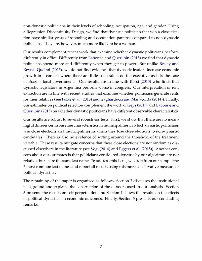
non-dynastic politicians in their levels of schooling, occupation, age, and gender. Usinga Regression Discontinuity Design, we find that dynastic politician that win a close elec-tion have similar years of schooling and occupation patterns compared to non-dynasticpoliticians. They are, however, much more likely to be a woman.

Our results complement recent work that examine whether dynastic politicians performdifferently in office. Differently from Labonne and Querubin (2015) we find that dynasticpoliticians spend more and differently when they get to power. But unlike Besley andReynal-Queirol (2015), we do not find evidence that dynastic leaders increase economicgrowth in a context where there are little constraints on the executive as it is the caseof Brazil’s local governments. Our results are in line with Rossi (2015) who finds thatdynastic legislators in Argentina perform worse in congress. Our interpretation of rentextraction are in line with recent studies that examine whether politicians generate rentsfor their relatives (see Folke et al. (2015) and Gagliarducci and Manacorda (2014)). Finally,our estimates on political selection complement the work of Geys (2015) and Labonne andQuerubin (2015) on whether dynastic politicians have different observable characteristics.

Our results are robust to several robustness tests. First, we show that there are no mean-ingful differences in baseline characteristics in municipalities in which dynastic politicianswin close elections and municipalities in which they lose close elections to non-dynasticcandidates. There is also no evidence of sorting around the threshold of the treatmentvariable. These results mitigate concerns that these close elections are not random as dis-cussed elsewhere in the literature (see Vogl (2014) and Eggers et al. (2015)). Another con-cern about our estimates is that politicians considered dynastic by our algorithm are notrelatives but share the same last name. To address this issue, we drop from our sample the7 most common last names and report all results using this more conservative measure ofpolitical dynasties.

The remaining of the paper is organized as follows. Section 2 discusses the institutionalbackground and explains the construction of the datasets used in our analysis. Section3 presents the results on self-perpetuation and Section 4 shows the results on the effectsof political dynasties on economic outcomes. Finally, Section 5 presents our concludingremarks.

3

2 Institutional Background and Data

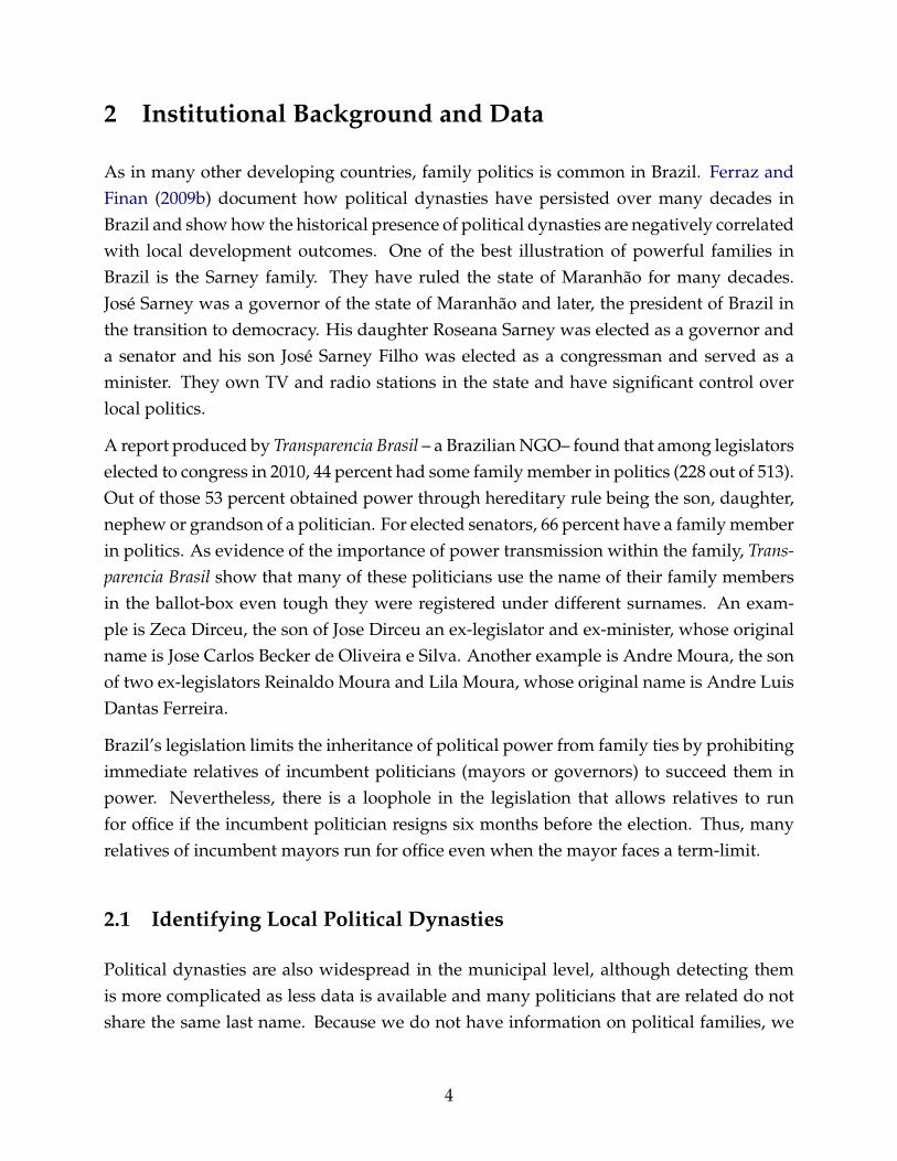
As in many other developing countries, family politics is common in Brazil. Ferraz andFinan (2009b) document how political dynasties have persisted over many decades inBrazil and show how the historical presence of political dynasties are negatively correlatedwith local development outcomes. One of the best illustration of powerful families inBrazil is the Sarney family. They have ruled the state of Maranhão for many decades.José Sarney was a governor of the state of Maranhão and later, the president of Brazil inthe transition to democracy. His daughter Roseana Sarney was elected as a governor anda senator and his son José Sarney Filho was elected as a congressman and served as aminister. They own TV and radio stations in the state and have significant control overlocal politics.

A report produced by Transparencia Brasil – a Brazilian NGO– found that among legislatorselected to congress in 2010, 44 percent had some family member in politics (228 out of 513).Out of those 53 percent obtained power through hereditary rule being the son, daughter,nephew or grandson of a politician. For elected senators, 66 percent have a family memberin politics. As evidence of the importance of power transmission within the family, Trans-parencia Brasil show that many of these politicians use the name of their family membersin the ballot-box even tough they were registered under different surnames. An exam-ple is Zeca Dirceu, the son of Jose Dirceu an ex-legislator and ex-minister, whose originalname is Jose Carlos Becker de Oliveira e Silva. Another example is Andre Moura, the sonof two ex-legislators Reinaldo Moura and Lila Moura, whose original name is Andre LuisDantas Ferreira.

Brazil’s legislation limits the inheritance of political power from family ties by prohibitingimmediate relatives of incumbent politicians (mayors or governors) to succeed them inpower. Nevertheless, there is a loophole in the legislation that allows relatives to runfor office if the incumbent politician resigns six months before the election. Thus, manyrelatives of incumbent mayors run for office even when the mayor faces a term-limit.

2.1 Identifying Local Political Dynasties

Political dynasties are also widespread in the municipal level, although detecting themis more complicated as less data is available and many politicians that are related do notshare the same last name. Because we do not have information on political families, we

4

exploit the structure of Brazilian surnames to build a proxy for political dynasties. Thename of a Brazilian citizen is composed of:

First Name Mother’s Last Name Father’s Last Name,

In most cases, Mother and Father’s Last Name are the last name inherited from theirrespective fathers. But married women can choose to maintain their name or add to theiroriginal name their husband’s last name, in which case their name will take the form of:

First Name Mother’s Last Name Father’s Last Name Husband’s Last Name.

We assume that politicians that have a common last name belong to the same family. Wethen match each candidate’s surname with the surnames of the mayors both in previousand in future elections. This matching procedure enables us to build two measures used inour analysis. The first is an indicator for dynastic persistence which equals one for politi-cians whose relatives are in office in the same municipality in the future (P). The secondis an indicator for a dynastic candidate which equals one if the candidate had a relativein office in the past (D). The former variable is used to assess the effect of incumbency ondynastic persistence, while the latter is used to investigate the consequences of politicaldynasties. Both analysis are based on the empirical strategies used previously by Dal Bóet al. (2009) and Querubin (2013).

The variables P and D are constructed matching surnames of all candidates for mayorin the 1996, 2000, 2004, 2008, and 2012 municipal elections with the surnames of electedmayors for the period 1988 to 2012. The variable P can be constructed for 1996 to 2008as its construction requires information of at least one subsequent election. On the otherhand D is constructed for 1996 to 2012 elections, as 1996 is the first year where we haveinformation on the last name of all candidates for office.4

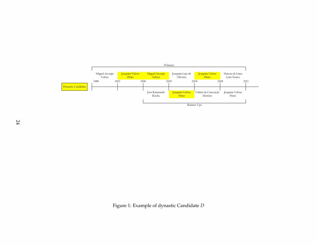
To illustrate our matching procedure we display an example in Figure 1 for the municipal-ity of Felício do Santos in the state of Minas Gerais. Our algorithm identifies Joaquim VelosoPinto, the elected mayor in 1992 and 2004 and the runner-up in 2000, as dynastic becausehe shares a surname name with Miguel Arcanjo Veloso who was in office between 1988 and1992. Miguel Arcanjo Veloso is elected for office again in 1996 and our algorithm identifieshim as dynastic because he shares a surname with Joaquim Veloso Pinto.

Figure 2 illustrates the construction of our persistence measure P. We consider MiguelArcanjo Veloso, elected candidate in the 1996 elections, a politician that is able to make

4The 1988 election was the first municipal election to take place after Brazil transitioned from dictator-ship to democracy. For the 1988 and 1992 elections, we only have the name of the elected mayor.

5

his dynasty persist since he shares his last name with Joaquim Veloso Pinto, who was themayor between 2004 and 2008. However, Jose Raimundo Rocha, the runner up in the sameelectoral race, is not considered to form part of a dynasty, as he does not share a surnamewith candidates elected in the subsequent electoral races.

The previous figures also display some of the challenges in constructing the measures ofpolitical dynasties. First, composite names are common in Brazil and it is important not tomistake them for surnames. In Joaquim Luiz Oliveira, Joaquim Luiz is the name and Oliveirathe surname, whereas, in Joaquim Veloso Pinto, Joaquim is the name and Veloso and Pintoare two different surnames. We adapted the algorithm to consider these cases and thenchecked its accuracy manually for more than 10,000 observations. Also, our algorithmdoes not code candidates as having a relative in office in the future or in the past if thecandidate shares the surname with himself. Thus, our measure of dynasties does notinclude the same candidate running for office in the future.

While we are able to detect a large number of dynastic candidates with our matching pro-cedure, it is important to note that measurement error still remains for two reasons. Thefirst is that individuals who share the same last name might not be relatives. The fact thatdynasties are restricted to the municipal-level reduces this concern since the median mu-nicipal population is around 10,000 inhabitants, and only a small share of the populationis involved in local politics. Nevertheless, it is still possible that some of the matches donot identify relatives. To address this issue, we drop matchings based on the seven mostcommon surnames in our data and show that our results are robust to this more strictmeasure. A second concern with the matching procedure is that politicians with differentlast names might actually be relatives. This could be the case of the wife of a politician,her cousin and nephews who might have different names even tough they are related. Ifthis is common, we might be underestimating the incidence of local political dynasties.

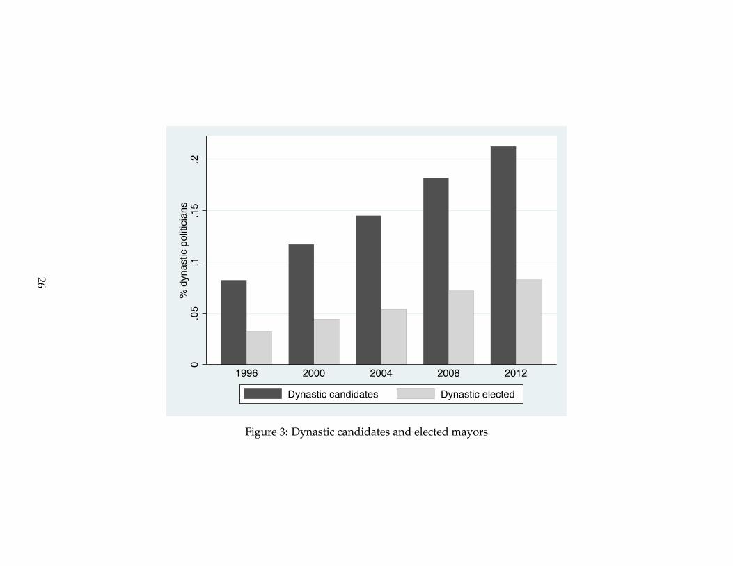
In Figure 3 we show the distribution of dynastic candidates and those elected for mayoroffice from 1996 to 2012. The share of dynastic candidates and those elected increase overtime because we have a short-panel to measure this type of persistence. In 2012 more than20 percent of candidates for mayor are dynastic and among the candidates, almost half ofthem get elected as mayors.

6

2.2 Municipal Governments in Brazil

Our study focuses on political dynasties at the municipal level. Municipalities are thesmallest administrative division in Brazil and they are responsible for the provision ofa broad set of public goods and services such as elementary schools, health clinics, andmost urban infrastructure projects such as road building and sanitation. Municipal gov-ernments finance the provision of public services through taxes collected at the local leveland transfers from the state and federal governments. Transfers represent the largestshare of government revenues, especially in small municipalities with limited bureau-cratic structure and tax capabilities. Some of these transfers are defined in constitutionalrules, whereas others are discretionary and result from a bargaining process between localofficials and state and federal officials.5

Brazilian municipalities are governed by a mayor (Prefeito) and local legislature (Camarade Vereadores) elected for a four-year term. While local legislators can get reelected indef-initely, mayors face a two-term limit.6 Mayors are responsible for proposing a budget,negotiating partnerships with state and federal governments and managing the provisionof public services. They are monitored by local legislators (Vereadores) who vote on themunicipal budget and legislate on local affairs concerning taxation, public policies andurban organization. Therefore, their support is essential to enable mayors to implementpublic policies.7

Corruption and the mismanagement of public resources are one of the main challengesfaced by Brazil’s local governments. There is widespread embezzlement of resources thatshould go to education, health, and urban infrastructure. Electoral incentives and thepotential for punishment of corrupt mayors in the polls play an important role to gener-ate accountability. However, political power induced by political dynasties might gener-ate incumbency effects that allow family politicians to mismanage resources and stay inpower.8

5See Arretche (1999) and Afonso and Araújo (2000) for an overview of municipalities’ responsibilitiesand financial structure.

6Mayors were allowed to run for reelection starting in the 2000 election.7See Ferraz and Finan (2009a) for more details on the performance of local legislators in Brazil.8See Ferraz and Finan (2011); Ferraz and Finan (2008); and Brollo et al. (2013) for evidence on how

electoral incentives interact with corrupt practices in Brazil.

7

2.3 Data Sources

We use electoral data for 5 municipal elections, from 1996 to 2012, obtained from the Fed-eral Electoral Commission (Tribunal Superior Eleitoral). The data includes information onall candidates running for office in municipal elections, the votes they obtained and theircharacteristics such as gender, schooling, age, and previous occupation. Starting in 2004,we also have information on campaign spending for each candidate. Our data includesmore than 15,000 candidates for mayor in each municipal election in more than 5,300 mu-nicipalities. The specific number of observations varies across elections since the numberof candidates and the number of municipalities change over time. Prior to 1996, detailedelectoral data is not available from the Federal Electoral Commission. Thus we gatheredinformation from the State Electoral Commissions (Tribunais Regionais Eleitorais) on thename of mayors elected in 3,800 municipalities in 1988 and more than 4,800 municipali-ties in 1992. Our data covers 21 out of the 25 states in 1988 and 25 out of the 26 in 1992.

Our measures of government quality includes information on a variety of policies and out-comes. We start by gathering administrative data on government expenditures and rev-enues reported by municipalities to the Ministry of Finance (Secretaria do Tesouro Nacional).This dataset named FINBRA includes information on all revenues and spending for morethan 5,000 municipalities. We distinguish between capital expenditures (i.e. investment inbuildings and infrastructure) versus current expenditures (i.e. salaries of public servants).We also gather information on revenues classified as either arising from local taxes (i.e.taxes on property and services) or from transfers from the federal and state government(i.e. block grants). Information on different categories of expenditures, such as education,health, urban infrastructure, is obtained from the same source.

Because it is difficult to assess the quality of government from spending patterns due tothe possibility of corruption and mismanagement, we also put together information onoutcomes affected by government policies in the spirit of Caselli and Michaels (2013) andFerraz and Finan (2009a). First, we use municipal GDP estimates from Brazil’s statisticaloffice Instituto Brasileiro de Geografia e Estatastica to examine how dynastic politicians affectlocal economic growth. Second, we gather information on the number of firms, num-ber of employees, and salaries in the formal labor market both in the private and in thepublic sector from the RAIS, a matched employer-employee dataset administered by theBrazilian Ministry of Labour.

In order to map public spending into public goods provision, we gather data on educationand health outcomes as well as on local infrastructure. Information on education on class

8

size, age-grade-distortion, and Prova Brasil– the national standardized test score– comefrom Brazil’s Education Statistics Institute (INEP). From the Prova Brasil data, we computethe average test scores in language and mathematics and standardize based on an yearlybasis. From the educational census (Censo Escolar) administered by INEP, we compute theaverage class size and the age-grade distortion. All educational outcomes are calculatedfor fifth grade students enrolled in municipal schools. We use data from Prova Brasil forthe periods of 2007 and 2011 and data from the educational census for the periods 2007-2008 and 2011-2012. Thus measures of schooling outcomes are taken in the end of mayor’selectoral terms. The health outcomes are obtained from the Brazil’s public health system,the Datasus. We build measures of the share of pregnant women that had frequent pre-natal visits during pregnancy, the share of low weight births, and infant mortality. Foreach measure we compute the average for each electoral term (i.e. 2005 to 2008 and 2009to 2012).

Data on local infrastructure comes from the Brazilian census. We construct measures ofinfrastructure such as the percentage of households with paved roads, open sewage, andgarbage collection. This data is just available for the 2010 census. We also use data fromthe Brazilian census to gather information on basic demographics at the baseline suchas population, urbanization, income per capita, and schooling. We compute the baselineinformation using data from the 2000 census.

In most of our estimations we use per capita measures based on estimates of the local pop-ulation provided by Brazil’s statistical office (Instituto Brasileiro de Geografia e Estatastica).We average all the variables throughout the electoral term whenever there is informationfor more than one period of each term. The appendix provides additional information onthe sources and the construction of all variables used throughout the paper.

3 Political Power Persistence

We begin our analysis by testing whether political power increases the likelihood of hav-ing a relative in office in the future. Because politicians that win and lose elections aredifferent in many dimensions such as their talent, wealth, and political capital, a sim-ple OLS regression will yield a biased coefficient on the probability of posterior politicalpower. Also, to the extent that personal characteristics persist within families, these differ-ences can create a positive association between winning an election and having a relativein office even in the absence of dynastic persistence (Dal Bó et al., 2009).

9

Hence, we follow Dal Bó et al. (2009) and Querubin (2013) and use a Regression Disconti-nuity Design to estimate the persistence in political power. We examine whether winnersin close elections have a higher probability of having a relative in office in the future com-pared to runner-ups using the following linear model:

Pimt = a + bWim + f (vim) + #imt, (1)

where Pimt is a indicator variable for whether candidate i in municipality m has a relativein office in year t, Wim is an indicator for whether candidate i won the election in munic-ipality m in 1996, and f (vim) is a function of the running variable vim that represents themargin of victory of candidate i in municipality m for the 1996 election.

Following Imbens and Lemieux (2008) and Lee and Lemieux (2010), our preferred spec-ification is based on a local linear regression using Imbens and Kalyanaraman (2012) toselect the optimal bandwidth. We estimate the model for observations within the band-width using a linear spline. As an alternative specification, we approximate the controlfunction using a fourth order polynomial with splines and restrict the analysis to obser-vations with winning margins between -0.5 and 0.5.

Because there is a legislation in Brazil that prohibits mayors’ direct relatives from suc-ceeding him in office, winners should have a mechanical lower probability of having arelative in office compared to their runner-ups in the following election. Moreover, may-ors can run for reelection hence the effect of power persistence might only appear in thefollowing election. Thus it is important to estimate persistence over several subsequentelections.

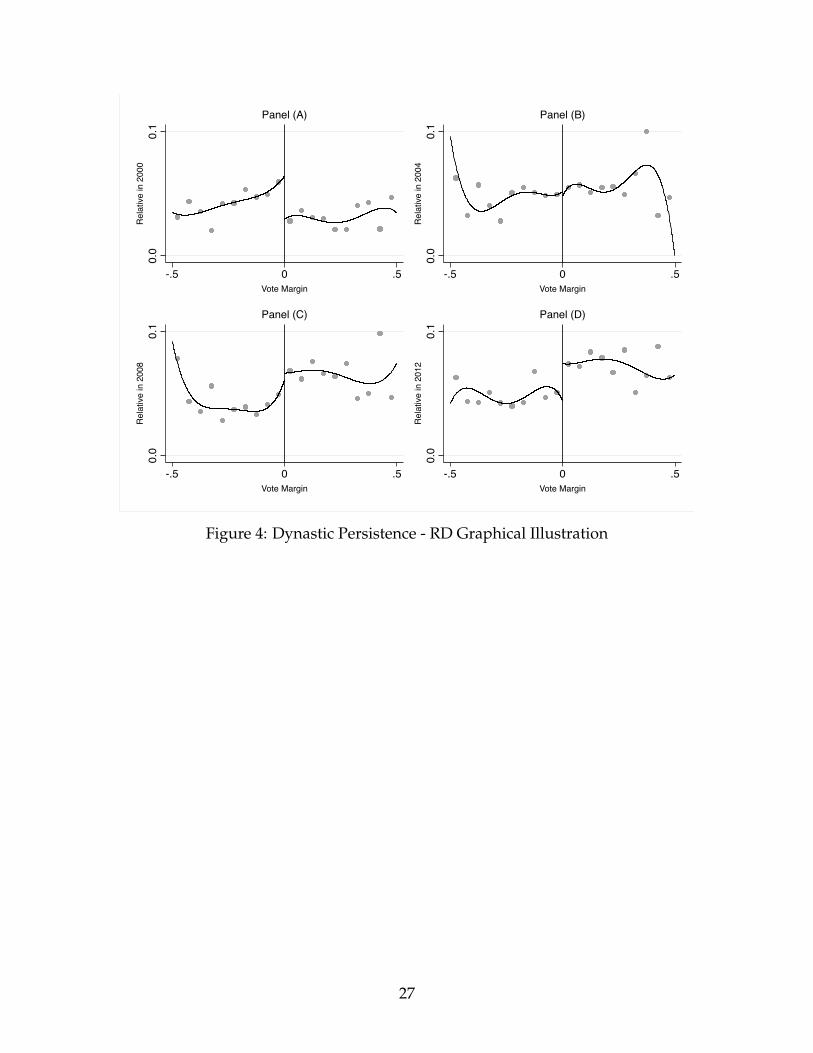
Figure 4 presents a graphical description of the results on dynastic persistence for foursubsequent election: 2000, 2004, 2008 and 2012. Each figure depicts the proportion ofrelatives in office in the future against the vote margin of the candidate in the 1996 mu-nicipal election using bins of 5 percent vote shares using a quartic polynomial fit of therelationship between dynastic persistence and vote margin.

Panel (A) reveals a negative relationship between the candidate winning the 1996 electionand a relative succeeding him in the 2000 election. This result is due to the fact that win-ners themselves can run for reelection in 2000 and even if mayors decide not to run forreelection, relatives cannot run. Panels (B) and (C) depict the same relationship for the2004 and 2008 elections. While there is no effect for the 2004 election (Panel B), the ef-fect seems positive but small for the 2008 election (Panel C). But these discontinuities aresmall and there is no evident dynastic persistence either after two or three electoral races.

10

In Panel (D), on the other hand, we observe a positive and significant dynastic persistenceafter four electoral races. Candidates who won a close election in 1996 are more likely tohave a relative elected for office in 2012 compared to candidates who lost a close electionin 1996. These results indicate that political power of families persist over time, confirm-ing that the results from other settings such as the United States and the Philippines arealso present in the context of Brazil (see Dal Bó et al. (2009) and Querubin (2013)).

Table 1 reports the RD estimates of political persistence. Columns 1 and 2 present themean of the persistence variable in each subsequent election among the candidates whowon and lost the 1996 municipal election, respectively. The probability of a relative ofthe winner to be in office increases over time from 3% in 2000 to 7.2% in 2012, while theprobability of a relative of the runner-up to be in office remains constant around 4.5%across all periods.

Column 3 depicts the difference in the means reported in the previous columns. The coef-ficient is negative in 1.8 percentage points for 2000, consistent with the fact that relativesof the winners in 1996 are not allowed to run in 2000. The estimate becomes positive in2000 and remains positive in 2004 and 2008. The magnitudes increase from 0.8 percentagepoints in 2004 to 2.5 percentage points in 2004 and 2.4 percentage points in 2008. Thesestatistics alone suggest that there are substantial differences in persistence over time be-tween winning and losing candidates. However, as we discussed before, these differencescan either reflect incumbency advantage or innate differences in political capital acrossfamilies.

Columns 4 and 5 present RD estimates comparing candidates who won or lost close elec-tions. To the extent that close elections are random, these candidates are similar in bothobservable an non-observable aspects and the comparison between these groups reflectsdynastic persistence. Column 4 reports local linear regression estimates using the Imbensand Kalyanaraman (2012) optimal bandwidth and column 5 reports polynomial splineestimates using a fourth order polynomial and a 0.50 bandwidth.

The estimates for persistence in 2000 confirm the intuition of the mean comparisons. Rel-atives of the winning candidates in 1996 are less prone to be in office in 2000 than relativesof losing candidates in 1996. However, the estimates for persistence in 2004 and 2008are quite different from the ones from column 3. These findings confirm the graphicalintuition of no persistence in these periods and indicate that the mean differences reflectdifferences in talent, drive and political capital across families and not dynastic persis-tence. The RD estimates for the last period confirm the intuition of persistence after some

11

periods. The likelihood of a relative of the winning candidate in 1996 to be elected in 2012is 2.8 percentage points. The magnitude of the coefficient is substantial and suggests thatbeing in office increases the likelihood of having a relative in office in the future in almost60 percent.

The results presented above suggest that dynastic persistence is relevant in our data, asit creates electoral advantages to members of certain families. This raises concerns aboutelectoral competition and political incentives which justifies investigating the effects ofthese families on government policies.

4 The Effects of Dynastic Politicians on Policies

In the previous section we showed that politicians that are elected by a small margin aremore likely to have a family member in office in the future. While this type of politicalpersistence might reduce political competition and compromise the functioning of democ-racies, it is unclear whether it has negative consequences for the way local governmentsare run. In this section we assess whether dynastic politicians behave differently in powerwhen compared to non-dynastic politicians and whether this affects economic outcomessuch as GDP and employment.

We start by showing in Table 2 the characteristics of localities where political dynastiesare present compared to those without political dynasties. All characteristics are drawnfrom the 2000 population census. Municipalities that have dynastic mayor are smaller,more urban, have a less educated population, and are poorer in terms of GDP per capita.They are less likely to have local institutions that can foster accountability such as localmedia (i.e. radio) and judiciary courts. All these differences are statistically significant andsome of the differences are sizable. Thus a simple comparison of policies and economicoutcomes between municipalities with and without dynastic politicians will yield biasedestimates of the effects of dynasties. Weak local institutions might drive both the existenceof political dynasties and the incentives to adopt bad policies.

We circumvent this potential bias using a Regression Discontinuity Design where we com-pare outcomes in municipalities where a dynastic candidate won by a small to those wherea dynastic lost by a small margin. Our empirical strategy is based on the assumption thatclose elections provide variation that is as good as random allowing us to control for ob-servable and unobservable municipal characteristics that might differ between localities

12

with and without a dynastic politician.9 Specifically, we estimate the following linear re-gression:

ymt = a + gDmt + f (vmt) + dXm + lt + #mt (2)

where ymt is the policy or economic outcome of municipality m during the electoral termt, Dmt is an indicator for whether the municipality is governed by a dynastic mayor (i.e.someone who belongs to the same family of a politician that has been in power previ-ously), Xm is a set of pre-determined municipal characteristics such as population andincome per capita, lt is a time dummy and #mt is an error term. The variable vmt is the dif-ference in vote share between the dynastic and the non-dynastic candidate and it is usedas the running variable in all specifications. The function f (.) is a smooth function of themargin of victory and includes an interaction between the dynastic indicator Dmt and themargin of victory vmt. The parameter of interest g captures the difference in policy y inmunicipalities with and without a dynastic mayor.

We estimate our model with two different econometric specifications: our main results arebased on a local linear regression using observations for an optimal bandwidth based onImbens and Kalyanaraman (2012). In this specification, we allow f (vmt) to vary in eachside of the discontinuity. We also report results from estimating a fourth order polyno-mial with a spline in each side of the discontinuity. We include election fixed effects anda set of pre-determined municipal characteristics as controls to gain precision, but all re-sults are robust to models where we do not control for municipal characteristics. In allspecifications standard-errors are clustered at the level of the municipality.

The model described above is estimated using data for the 2004 and 2008 municipal elec-tions and for each election we identify dynastic candidates as the ones with relatives inoffice in previous mandates. We restrict our sample to outcomes for the 2005-2008 and2009-2012 mandates because these are the periods for which we can measure dynastiesusing four previous elections and we have data on economic outcomes for the whole elec-toral term. We exclude from our sample municipalities in which dynastic candidates wereneither the winner nor the runner-up and municipalities in which both the winner and therunner-up are dynastic.

Under this application of the Regression Discontinuity Design, it is important to noticetwo things. First, the estimated effects represent local estimates of dynastic politicians oneconomic outcomes for municipalities that are highly competitive. These effects might bequite different in localities where dynasties win by a large vote margin. From a theoretical

9See Lee (2008) for the original application of Regression Discontinuity to elections.

13

perspective, it is unclear whether the RD estimates are larger or smaller than average ef-fects. On the one hand, political dynasties facing less electoral competition can be less ac-countable and therefore perform worse than dynasties facing a lot of competition. On theother hand, if voters select the best families into power, political dynasties facing less elec-toral competition could be the ones with better performance.10 In the appendix we presentestimates on the effects of political dynasties using an alternative econometric specifica-tion that does not rely on close-elections. We estimate difference-in-difference modelsexploiting changes in policies in municipalities that elect a dynastic politician comparedto those municipalities that do not elect a dynastic politician.

A second concern is that, while the RD design controls for unobserved characteristics atthe municipal level, it cannot control for unobserved characteristics of politicians, parties,or efforts of mobilization. Because dynastic politicians have a natural incumbency ad-vantage (see Dal Bó et al. (2009) and Querubin (2013)), a dynastic candidate that barelywins an election might be, on average, worse than an average candidate. Thus, we mightbe comparing candidates with different quality.11 In order to shed light on this selectionmechanism, we analyze in section 4.3 whether elected dynastic candidates are different inobservable characteristics.

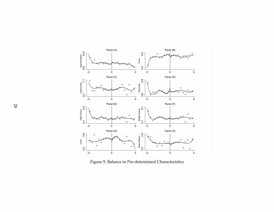
Before showing the results, we present evidence that indeed our RD design can be con-sidered as good as random in terms of municipal characteristics. We use pre-determinedmunicipal characteristics such as population, proportion of rural households, and incomeper capita for either 1999 or 2000– at least 4 years before the dynastic election occurs–and test whether they exhibit a discontinuity. Figure 5 provides evidence that municipalcharacteristics are smooth in the discontinuity that determine whether the municipalityis governed by a dynastic politician. Each panel plots an outcome averaged in 5 percentbins against the vote margin of the dynastic candidate. The panels also report a quar-tic polynomial fit of the relationship between the outcome and vote margin. In TableA1 in the Appendix we report estimates of these discontinuities using both a local lin-ear regression using the Imbens and Kalyanaraman (2012) bandwidth (Panel A) and aquartic polynomial spline for a 0.50 bandwidth. The results confirm the graphical intu-ition that pre-determined variables are balanced around the winning margin threshold.We complement the analysis on pre-determined characteristics with a test of sorting inthe discontinuity. In localities where institutions are weak, dynastic politicians might bemore likely to commit some type of electoral fraud and affect electoral outcomes in very

10See Besley and Reynal-Queirol (2015).11See Vogl (2014) for a related point made for black mayors in the US.

14

close elections. This would invalidate the comparison of close-elections between dynasticand non-dynastic candidates as a quasi-randomized empirical strategy. We test for thepotential manipulation of elections around the discontinuities using the test proposed byMcCrary (2008). In Figure 6, we plot the densities of the vote margin and find no evidenceof manipulation of the winning margin by dynastic candidates.

4.1 Political Dynasties and Government Expenditures

We start our analysis by examining whether there are differences in public spending be-tween dynastic and non-dynastic mayors. Figure 7 presents graphical evidence on theeffect of political dynasties on the overall pattern of government expenditures and aggre-gated categories such as capital versus current expenditures. As we can observe in thefigures, dynastic politicians do not seem to chose different levels of government spendingcompared to non-dynastic politicians in similar municipalities. But these politicians doseem to spend more on capital rather than current expenditures.

The regression results for these variables using different Regression Discontinuity specifi-cations are presented in Table 3. Panel (A) reports local linear regression estimates usingthe Imbens and Kalyanaraman (2012) optimal bandwidth and Panel (B) presents fourthorder polynomial spline estimates using a 0.50 bandwidth. All estimates include timefixed-effects and municipal controls to improve precision. Standard-errors are clusteredat the municipality level. The coefficient in column (1) suggests that dynastic mayorsspend, on average, 8 percent more than non-dynastic mayors. This corresponds to an in-crease of R$124 to R$149 in expenditures per capita with respect to an average of R$1700.12

Columns (2) and (3) provide evidence that the increase in expenditures is higher in capitalthan in current expenditures. Dynastic mayors spend, on average, 16 percent more oncapital expenditures compared to non-dynastic mayors. These mayors also spend moreon current spending, but the difference is much smaller (4.7 percent) and the effect is non-significant in the polynomial specification.

Given that dynastic mayors spend more resources, we examine the source for these ad-ditional expenditures. Brazilian municipalities have two main sources of financing: localtaxes and transfers from the central government.13 Columns (4) and (5) test whether dy-nastic mayors collect more taxes and receive more transfers from the central government.We find that dynastic mayors receive, on average, 6 to 7 percent more transfers from the

12All values are deflated to December 2012. The average R$ to US$ exchange rate was 2.08.13The possibility of running a deficit is limited under Brazil’s fiscal responsibility law.

15

central government compared to non-dynastic mayors. The effects on taxes are similarin magnitude but not significant. Because approximately 65 to 70 percent of municipalrevenues come from transfers, we conclude that capital expenditures are mainly financedthrough more transfers from the central government.

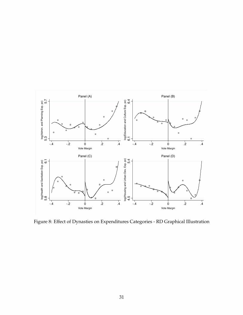
Next, we examine in which areas local governments increase expenditures. Figure 8 pro-vides a graphical illustration of the effect of political dynasties on the four most importantcategories of spending: administration and planning, education and culture, healthcareand sanitation and housing and urban development. Dynastic politicians seem to spendmore on health and sanitation and housing and urban development, expenditures that areintensive in public works. Table 3 provides regression results for the four categories pre-sented in the figure as well as for social assistance and transportation. Together these sixcategories comprise more than 90 percent of total expenditures. Dynastic mayors spendmore resources in education, health, urban development, and public transportation. Theeffects range from a 6 percent increase in education to a 57 percent increase in transporta-tion. While the effect for education loses significance in the polynomial splines, all theother coefficients are robust to the alternative specifications. In terms of magnitudes, thelargest differences are in urban development and health. Combined these categories cor-respond to a large share of government spending. These categories also include significantspending in public works such as building housing for poor families, urban infrastructure,health clinics, and sanitation.14

4.2 Political Dynasties, Economic Performance, and Public Goods

Our previous findings suggest that dynastic politicians increase the size of local govern-ments, mostly through increases in infrastructure spending. We next examine whethermunicipalities that elect a dynastic politician perform better in terms of economic per-formance and whether the increase in government spending affects the quality of publicservices. We first use measures of municipal GDP growth and measures of growth in em-ployment and the number of firms to examine economic performance. We then assessthe quality of public services using data on education, health and urban infrastructure.We chose these three sectors because they correspond to most of the spending decidedby local mayors and because these are the sectors in which we have shown that dynasticmayors spend more resources.

14In the appendix we test for the robustness of our findings for alternative bandwidths and functionalforms.

16

The effects of a dynastic politician on economic performance using the regression Discon-tinuity Design from equation (2) are shown in Table 5. We present results from estimatinga local linear regression with an optimal bandwidth (Panel A) and a quartic polynomial(Panel B). In columns (1) to (4) we show the effects on municipal GDP growth over theelectoral term (four years). Municipalities grow on average 24 percent over a four yearperiod. But we do not find significant differences in growth rate in localities where a dy-nastic politician won by a small margin compared to places where he/she lost by a smallmargin. These localities, despite higher spending in infrastructure, do not grow more. Wethen split growth into different sectors and estimate separate regressions for growth inagriculture, manufacturing, and services. We do not find any differences in performanceacross these localities. Finally, in columns (5) and (6) we show that localities with a dy-nastic politician do not seem to have a different performance in the labor market either. Incolumn (5) we find that municipalities with dynastic mayors do not grow more in terms ofemployment (column (5)) or in terms of number of firms (column (6)). The lack of effectsin economic performance are robust to different specifications, as those shown in Panel (B)where we estimate the RD model with a quartic polynomial. Alternative specifications inthe appendix support this conclusion. Overall we find not evidence of a differential eco-nomic performance of dynastic mayors.

We next examine whether dynastic mayors affect the quality of public services. The re-sults shown in Table 6 focus on outcomes for education, health and urban infrastructure.The first three columns show the results for education. We start by examining whetherdynastic mayors use resources in education to reduce class size. Spending more on ed-ucation could reduce class size through the construction of new classrooms and schoolsand through the hiring of additional teachers. We find that, despite a negative point esti-mate, municipalities with a dynastic mayor do not have significant smaller average classsizes for primary school children compared to municipalities without a dynastic mayor.The point estimate is very small suggesting no difference between municipalities with andwithout dynastic mayors. We next examine two different measures of educational quality.In column (2) we look at the age-grade distortion measured by the percentage of studentsthat are lagging behind when comparing their grade to their age. In column (3) we lookat test scores in a standardized national exam for 5th grade in Math and Portuguese.15 Wefind that despite spending more resources in education, dynastic mayors do not improveeducational outcomes in terms of both age-grade distortion and test scores.

Columns (4) to (6) investigate outcomes related to health. We follow Fujiwara (2015) and

15We use as outcomes the average of both grades standardized.

17

use information on the share of pregnant women with more than 7 prenatal visits (column4) and the share of babies born with low birth weights (column 5). Fujiwara (2015) pro-vides evidence that these health outcomes are responsive to short-term changes in poli-cies and thus we would expect the changes in expenditures to improve these outcomes.Finally in column (6) we test whether infant mortality differs in municipalities that electa dynastic mayor. Overall we find small point estimate and no significant differences inhealth outcomes between municipalities with and without a dynastic mayor despite thatlarger expenditures in health care.

The three last columns in Table 6 look at urban infrastructure. Because we only have in-dicators for the 2010 census, we test for different levels of urban infrastructure for mayorselected in the 2008 election. We look at the percentage of households that live in a local-ity with paved roads, open sewage, and garbage in the streets. These variables can bedirectly affected by mayors as they are responsible for these types of public goods. Wedo not find any difference between these three measures of urban infrastructure in mu-nicipalities that elected a dynastic mayor in close elections and those that did not despitethe larger sums of capital expenditures targeted at urban infrastructure in these localities.Overall, we conclude that despite spending more resources on capital expenditures, andin particular health and urban infrastructure, dynastic mayors do not change the qualityof these public services.

In sum, dynastic mayors spend significantly more resources in infrastructure comparedto non-dynastic mayors with no effects on economic growth, employment growth, or im-provements in the quality of a large number of public services. There are two direct in-terpretations of these findings. One potential interpretation is that dynastic mayors havesignificant political capital that allows them to divert resources and still remain politicallycompetitive. This explanation would be consistent with the results of Brollo et al. (2013)who find that Brazilian mayors that receive an exogenous increase in their budget can getreelected and extract rents from corruption. The pattern of increasing spending with nulleffects on public services is consistent with previous work by Caselli and Michaels (2013)and Monteiro and Ferraz (2010) who show that increasing revenues based on oil revenuesincreased municipal government spending but did not translate into improvements in thequality of public services.

An alternative explanation for the increase in spending with no improvements in eco-nomic performance and public services is that dynastic mayors are drawn from a worsepool of candidates. Under this explanation, dynastic mayors spend more with no effectsbecause of negative political selection. In the next section we examine this hypothesis

18

looking at whether elected dynastic mayors differ from non-dynastic mayors in observ-able characteristics such as years of schooling and occupation.

4.3 Political Dynasties and Selection

In this section we test whether dynastic mayors elected by a small margin differ from non-dynastic mayors in four characteristics that have been shown to affect policy outcomes:education, occupation, age, and gender. We focus on close elections where a dynasticmayor competes against a non-dynastic mayor and estimate a series of regressions usingboth a local linear regression and a polynomial spline specification similar to the onesused in the previous section. The results are presented in Table 7.

We start our analysis looking at whether dynastic politicians are less qualified than non-dynastic politicians. We use schooling and an indicator for whether the politician had ahigh skill occupation before the election as a proxy for political quality.16 We find that dy-nastic mayors elected in close-elections do not have different levels of schooling or highskill occupation compared to non-dynastic mayors. The point estimate for schooling incolumn (1) is 0.63 (standard-error=0.59) in the local linear regression specification and0.47 (standard-error=0.59) in the polynomial specification. Both coefficients are not statis-tically significant and represent less than a 5 percent difference in years of schooling withrespect to the mean education level of 12.4 years. The point estimates for high skill occu-pation displayed in column (2) are also small and not statistically significant for both thelocal linear specification displayed in Panel (A) and the quartic polynomial displayed inPanel (B). Hence, at least in terms of observable skills, dynastic politicians are not differentthan non-dynastic politicians elected in very competitive elections. This result is relatedto Geys (2015) who find no evidence of lower education levels among directly electeddynastic mayors in Italian localities.

We next turn to two other characteristics that might differ between dynastic and non-dynastic politicians: age and gender. Because politicians in Brazil face a term-limit aftertwo terms in office, we might expect incumbents to try to maintain political power byencouraging their wives and children to run for office. In Table 7, column (3), we showthe results for age. We find no statistically significant difference in age between dynasticand non-dynastic politicians. The point estimates vary from -0.76 to -1.39 and both arequite small when compared to 47, the average age of mayors. Finally, in column (4) wetest whether dynastic politicians are more likely to be a female. We find a large and robust

16See Ferraz and Finan (2009a), Brollo et al. (2013), and Besley et al. (2011) on use of education of leaders.

19

increase in probability of the mayor being female when a dynastic politician is elected in aclose-election. The point estimates range from 14 to 16 percentage points (standard errorsare 0.04 and 0.047 respectively) which represent a 100 percent increase in probability ofelecting a female mayors. This result is similar to the findings of Labonne and Querubin(2015) who show that in the Philippines a relatively high numbers of women elected asmayors are the result of dynastic women replacing mayors who face a term-limit.

5 Concluding Remarks

This paper uses data from Brazil’s local governments to examine whether dynastic mayorsimplement different policies compared to non-dynastic mayors. We circumvent empiricalconcerns that municipalities where dynastic mayors get elected are different from thoselocalities that do not elect dynastic mayors using a regression Discontinuity Design. Wecompare policies and performance of dynastic and non-dynastic mayors in similar mu-nicipalities and find that mayors that come from a family that had politicians in powerin previous periods spend more resources, specially in infrastructure projects. We find,however, that this additional spending does not induce more economic and employmentgrowth and does not improve the quality of urban infrastructure nor the quality of publicservices in education and health. We interpret our results as suggestive evidence that dy-nastic mayors, despite not implementing worse policies as many observers would argue,are likely to reduce the welfare of citizens by spending more resources without positiveconsequences.

20

References

Acemoglu, D. and Robinson, J. A. (2008). Persistence of power, elites, and institutions.American Economic Review, 98(1):267–293.

Afonso, J. R. R. and Araújo, É. A. (2000). A capacidade de gasto dos municípios brasileiros:arrecadação própria e receita disponível. Working Paper.

Arretche, M. T. (1999). Políticas sociais no brasil: descentralização em um estado federa-tivo. Revista brasileira de ciências sociais, 14(40):111–141.

Barro, R. (1973). The control of politicians: An economic model. Public Choice, 14(1):19–42.

Besley, T., Montalvo, J. G., and Reynal-Querol, M. (2011). Do Educated Leaders Matter?Economic Journal, 121(554):F205–.

Besley, T. and Reynal-Queirol, M. (2015). The logic of hereditary rule: Theory and evi-dence. Working Paper.

Brollo, F., Nannicini, T., Perotti, R., and Tabellini, G. (2013). The Political Resource Curse.The American Economic Review, 103(5):1759–1796.

Caselli, F. and Michaels, G. (2013). Do Oil Windfalls Improve Living Standards? Evidencefrom Brazil. American Economic Journal: Applied Economics, 5(1):208–38.

Dal Bó, E., Dal Bó, P., and Snyder, J. (2009). Political dynasties. The Review of EconomicStudies, 76(1):115–142.

Dal Bó, E. and Rossi, M. A. (2011). Term length and the effort of politicians. The Review ofEconomic Studies, 78(4):1237–1263.

Economist, T. (2015). Dynasties: The power of families.

Eggers, A. C., Fowler, A., Hainmueller, J., Hall, A. B., and Snyder, J. M. (2015). On thevalidity of the regression discontinuity design for estimating electoral effects: New evi-dence from over 40,000 close races. American Journal of Political Science, 59(1):259–274.

Ferraz, C. and Finan, F. (2008). Exposing corrupt politicians: The effects of Brazil’s publiclyreleased audits on electoral outcomes. The Quarterly Journal of Economics, 123(2):703–745.

Ferraz, C. and Finan, F. (2009a). Motivating politicians: The impacts of monetary in-centives on quality and performance. Technical report, National Bureau of EconomicResearch.

21

Ferraz, C. and Finan, F. (2009b). Political power persistence and economic development:Evidence from Brazil’s regime transition. Unpublished Manuscript.

Ferraz, C. and Finan, F. (2011). Electoral accountability and corruption: Evidence from theaudits of local governments. American Economic Review, 101:1274–1311.

Folke, O., Persson, T., and Rickne, J. (2015). Dynastic political rents. Columbia University.Mimeo.

Fujiwara, T. (2015). Voting technology, political responsiveness, and infant health: Evi-dence from brazil. Econometrica, 83(2):423–464.

Gagliarducci, S. and Manacorda, M. (2014). Politics in the family: Nepotism and the hiringdecision of Italian firms. Tor Vergata University. Mimeo.

Geys, B. (2015). Political dynasties, electoral institutions, and politicians’ human capital.Norwegian Business School BI. Mimeo.

Imbens, G. and Kalyanaraman, K. (2012). Optimal bandwidth choice for the regressiondiscontinuity estimator. The Review of Economic Studies, 79(3):933–959.

Imbens, G. W. and Lemieux, T. (2008). Regression discontinuity designs: A guide to prac-tice. Journal of Econometrics, 142(2):615–635.

Labonne, J., S. P. and Querubin, P. (2015). Political Dynasties, Term Limits and FemalePolitical Empowerment: Evidence from the Philippines. New York University. Mimeo.

Lee, D. S. (2008). Randomized experiments from non-random selection in U.S. Houseelections. Journal of Econometrics, 142(2):675–697.

Lee, D. S. and Lemieux, T. (2010). Regression discontinuity designs in economics. Journalof Economic Literature, 48:281–355.

McCrary, J. (2008). Manipulation of the running variable in the regression discontinuitydesign: A density test. Journal of Econometrics, 142(2):698–714.

Michels, R. (1915). Political parties: A sociological study of the oligarchical tendencies of moderndemocracy. Hearst’s International Library Company.

Monteiro, J. and Ferraz, C. (2010). Does oil make leaders unaccountable? evidence frombrazil’s offshore oil boom. Mimeo PUC-Rio.

Olson, M. (2002). The logic of collective action. Public goods and the theory of groups, 2.

Pareto, V. (1968). The Rise and Fall of the Elites: an Application of Theoretical Sociology.

22

Querubin, P. (2013). Family and politics: Dynastic incumbency advantage in the Philip-pines. Working Paper.

Rossi, M. A. (2015). Self-perpetuation of political power: Evidence from a natural experi-ment in Argentina. Universidad de San Andres. Mimeo.

Vogl, T. S. (2014). Race and the politics of close elections. Journal of Public Economics,109:101–113.

23

Winners

Joaquim Veloso Pinto

1988 1992

José Raimundo Rocha


Miguel Arcanjo Veloso

Runner-Ups

Dynastic Candidate

Valmir da Conceição Moreira


Mateus de Lima Leite Soares

2004 2008

Joaquim Luiz de Oliveira


20121996 2000


Figure 1: Example of dynastic Candidate D

24


Eloísa Helena Rocha Oliveira

2012 2016

Runner-Ups

José Raimundo Rocha


Valmir da Conceição Moreira


Persistent Dynasty


2000 2004 20081996

Winners


Joaquim Luiz de Oliveira


Figure 2: Example of dynastic persistence P

25

0.0

5.1

.15

.2%

dyn

astic

pol

itici

ans

1996 2000 2004 2008 2012

Dynastic candidates Dynastic elected

Figure 3: Dynastic candidates and elected mayors

26

0.0

0.1

Rel

ativ

e in

200

0

-.5 0 .5Vote Margin

Panel (A)

0.0

0.1

Rel

ativ

e in

200

4

-.5 0 .5Vote Margin

Panel (B)

0.0

0.1

Rel

ativ

e in

200

8

-.5 0 .5Vote Margin

Panel (C)

0.0

0.1

Rel

ativ

e in

201

2

-.5 0 .5Vote Margin

Panel (D)

Figure 4: Dynastic Persistence - RD Graphical Illustration

27

8.9

10.3

log(

Popu

latio

n)

-.5 0 .5

Panel (A)

0.2

0.5

Rur

al

-.5 0 .5

Panel (B)

6.7

7.1

log(

Inco

me)

-.5 0 .5

Panel (C)

0.8

0.9

Elec

trici

ty

-.5 0 .5

Panel (D)

0.1

0.2

Hig

h Sc

hool

-.5 0 .5

Panel (E)

0.1

0.1

Mid

dle

Scho

ol

-.5 0 .5

Panel (F)

0.2

0.6

Cou

rt

-.5 0 .5

Panel (G)

0.2

0.5

Rad

io S

tatio

n

-.5 0 .5

Panel (H)

Figure 5: Balance in Pre-determined Characteristics

28

01

23

-1 -.5 0 .5 1

Figure 6: Testing for Sorting in the Discontinuity

29

7.3

7.6

log(

Expe

nditu

res

pc)

-.4 -.2 0 .2 .4Vote Margin

Panel (A): Total Expenditures5.

05.

4lo

g(C

apita

l Exp

endi

ture

s pc

)

-.4 -.2 0 .2 .4Vote Margin

Panel (B): Capital Expenditures

7.2

7.4

log(

Cur

rent

Exp

endi

ture

s pc

)

-.4 -.2 0 .2 .4Vote Margin

Panel (C): Current Expenditures

Figure 7: Effect of Dynasties on Expenditures - RD Graphical Illustration

30

5.3

5.7

log(

Adm

in. a

nd P

lann

ing

Exp.

pc)

-.4 -.2 0 .2 .4Vote Margin

Panel (A)

6.1

6.4

log(

Educ

atio

n an

d C

ultu

re E

xp. p

c)

-.4 -.2 0 .2 .4Vote Margin

Panel (B)

5.8

6.1

log(

Hea

lth a

nd S

anita

tion

Exp.

pc)

-.4 -.2 0 .2 .4Vote Margin

Panel (C)

4.5

5.4

log(

Hou

sing

and

Urb

an D

ev. E

xp. p

c)

-.4 -.2 0 .2 .4Vote Margin

Panel (D)

Figure 8: Effect of Dynasties on Expenditures Categories - RD Graphical Illustration

31

Table 1: The Effect of Winning on the Presence of a Relative in Office in the Future

Mean

Winner Runner-Up

Difference Effect of winning

(1) (2) (3) (4) (5)

Relative Elected in 2000 0.030 0.047 -0.018*** -0.033*** -0.033**[0.002] [0.003] (0.004) (0.011) (0.014)

Bandwidth 0.101 0.50Observations 5,207 5,207 10,414 4,974 10,154

Relative Elected in 2004 0.054 0.046 0.008* 0.002 -0.003[0.003] [0.003] (0.004) (0.013) (0.015)


Relative Elected in 2008 0.065 0.040 0.025*** 0.010 0.005[0.003] [0.003] (0.004) (0.012) (0.015)


Relative Elected in 2012 0.072 0.047 0.024*** 0.028** 0.028*[0.004] [0.003] (0.005) (0.012) (0.016)


Specification - - - IK Band-width,Linear

50% band-width,QuarticPolyno-

mial

Notes: The unit of observation is a candidate in the 1996 municipal election. Sample is restrictedto the winners and runner-ups of the election. The dependent variable indicates whether a relativeof the candidate was elected for mayor in each subsequent period. Each cell in columns (1) and(2) reports the sample mean of the specified variable. Each cell in column (3) reports the differ-ence of columns (1) and (2). Each cell in column (4) reports the coefficient from a local linear re-gression using the Imbens and Kalyanaraman (2012) optimal bandwidth. Each cell in columns (5) re-ports the coefficient from a regression using a quartic spline. Details on the construction of all vari-ables are presented in the appendix. Standard errors are displayed in parentheses and standard de-viations in brackets. Significantly different than zero at 99 (***), 95 (**), 90 (*) percent confidence.

32

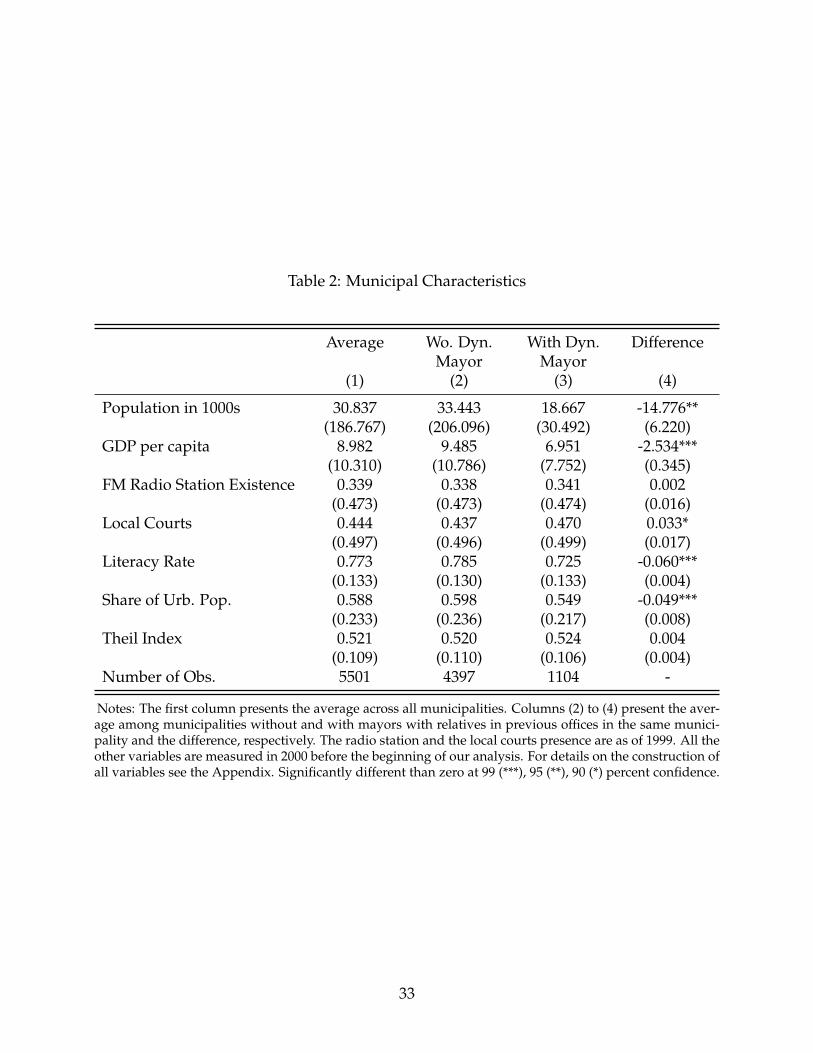
Table 2: Municipal Characteristics

Average Wo. Dyn.Mayor

With Dyn.Mayor

Difference

(1) (2) (3) (4)

Population in 1000s 30.837 33.443 18.667 -14.776**(186.767) (206.096) (30.492) (6.220)

GDP per capita 8.982 9.485 6.951 -2.534***(10.310) (10.786) (7.752) (0.345)

FM Radio Station Existence 0.339 0.338 0.341 0.002(0.473) (0.473) (0.474) (0.016)

Local Courts 0.444 0.437 0.470 0.033*(0.497) (0.496) (0.499) (0.017)

Literacy Rate 0.773 0.785 0.725 -0.060***(0.133) (0.130) (0.133) (0.004)

Share of Urb. Pop. 0.588 0.598 0.549 -0.049***(0.233) (0.236) (0.217) (0.008)

Theil Index 0.521 0.520 0.524 0.004(0.109) (0.110) (0.106) (0.004)

Number of Obs. 5501 4397 1104 -

Notes: The first column presents the average across all municipalities. Columns (2) to (4) present the aver-age among municipalities without and with mayors with relatives in previous offices in the same munici-pality and the difference, respectively. The radio station and the local courts presence are as of 1999. All theother variables are measured in 2000 before the beginning of our analysis. For details on the construction ofall variables see the Appendix. Significantly different than zero at 99 (***), 95 (**), 90 (*) percent confidence.

33

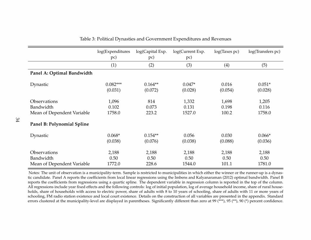
Table 3: Political Dynasties and Government Expenditures and Revenues

log(Expenditurespc)

log(Capital Exp.pc)

log(Current Exp.pc)

log(Taxes pc) log(Transfers pc)

(1) (2) (3) (4) (5)

Panel A: Optimal Bandwidth

Dynastic 0.082*** 0.164** 0.047* 0.016 0.051*(0.031) (0.072) (0.028) (0.054) (0.028)

Observations 1,096 814 1,332 1,698 1,205Bandwidth 0.102 0.073 0.131 0.198 0.116Mean of Dependent Variable 1758.0 223.2 1527.0 100.2 1758.0

Panel B: Polynomial Spline

Dynastic 0.068* 0.154** 0.056 0.030 0.066*(0.038) (0.076) (0.038) (0.088) (0.036)

Observations 2,188 2,188 2,188 2,188 2,188Bandwidth 0.50 0.50 0.50 0.50 0.50Mean of Dependent Variable 1772.0 228.6 1544.0 101.1 1781.0

Notes: The unit of observation is a municipality-term. Sample is restricted to municipalities in which either the winner or the runner-up is a dynas-tic candidate. Panel A reports the coefficients from local linear regressions using the Imbens and Kalyanaraman (2012) optimal bandwidth. Panel Breports the coefficients from regressions using a quartic spline. The dependent variable in regression column is reported in the top of the column.All regressions include year fixed effects and the following controls: log of initial population, log of average household income, share of rural house-holds, share of households with access to electric power, share of adults with 8 to 10 years of schooling, share of adults with 11 or more years ofschooling, FM radio station existence and local court existence. Details on the construction of all variables are presented in the appendix. Standarderrors clustered at the municipality-level are displayed in parentheses. Significantly different than zero at 99 (***), 95 (**), 90 (*) percent confidence.

34

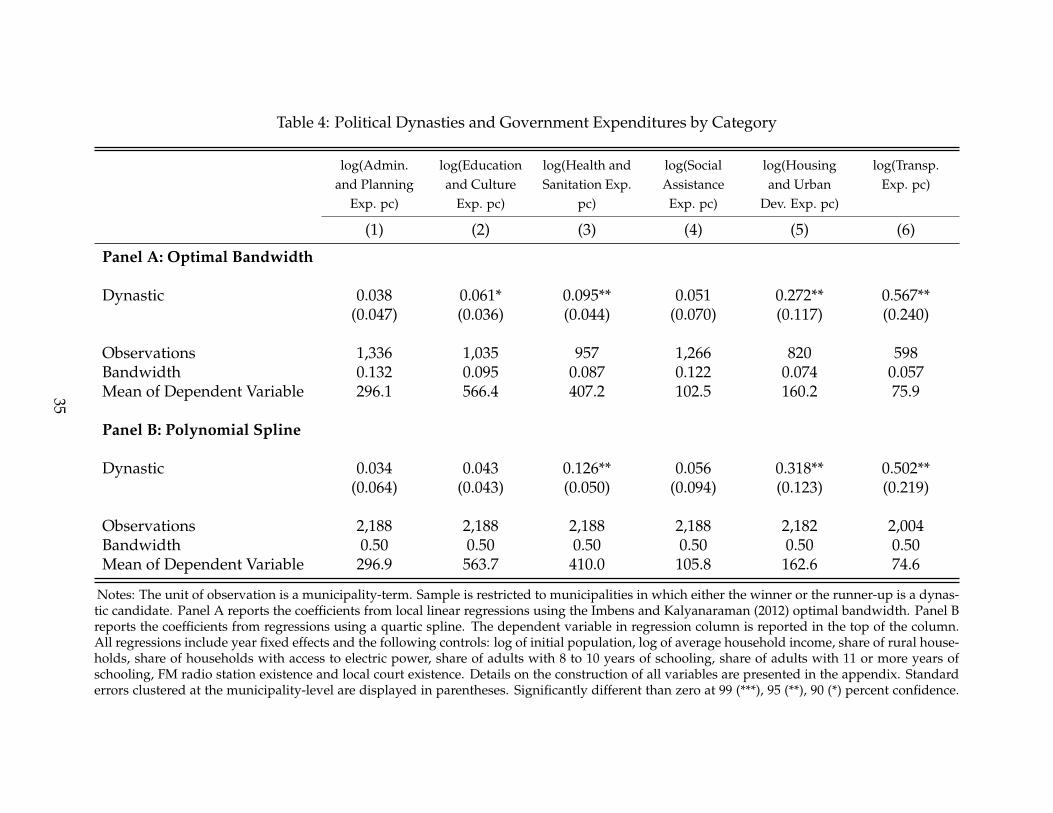
Table 4: Political Dynasties and Government Expenditures by Category

log(Admin.and Planning

Exp. pc)

log(Educationand Culture

Exp. pc)

log(Health andSanitation Exp.

pc)

log(SocialAssistance

Exp. pc)

log(Housingand Urban

Dev. Exp. pc)

log(Transp.Exp. pc)

(1) (2) (3) (4) (5) (6)


Dynastic 0.038 0.061* 0.095** 0.051 0.272** 0.567**(0.047) (0.036) (0.044) (0.070) (0.117) (0.240)

Observations 1,336 1,035 957 1,266 820 598Bandwidth 0.132 0.095 0.087 0.122 0.074 0.057Mean of Dependent Variable 296.1 566.4 407.2 102.5 160.2 75.9


Dynastic 0.034 0.043 0.126** 0.056 0.318** 0.502**(0.064) (0.043) (0.050) (0.094) (0.123) (0.219)

Observations 2,188 2,188 2,188 2,188 2,182 2,004Bandwidth 0.50 0.50 0.50 0.50 0.50 0.50Mean of Dependent Variable 296.9 563.7 410.0 105.8 162.6 74.6


35

Table 5: Political Dynasties and Economic Performance

GDP Growth AgriculturalGDP Growth

ManufacturingGDP Growth

Services GDPGrowth

No. ofEmployees

Growth

No. ofEstablishments

Growth

(1) (2) (3) (4) (5) (6)


Dynastic 0.014 0.059 -0.020 -0.001 -0.133 -0.053(0.036) (0.062) (0.080) (0.018) (0.222) (0.044)

Observations 1,003 967 670 1,556 1,643 1,144Bandwidth 0.091 0.088 0.059 0.171 0.193 0.109Mean of Dependent Variable 0.24 0.05 0.41 0.29 0.76 0.37


Dynastic 0.018 0.098 0.154 -0.013 -0.266 -0.046(0.037) (0.071) (0.182) (0.025) (0.295) (0.053)

Observations 2,188 2,186 2,188 2,188 2,142 2,186Bandwidth 0.50 0.50 0.50 0.50 0.50 0.50Mean of Dependent Variable 0.24 0.05 0.47 0.29 0.74 0.35


36

Table 6: Political Dynasties and the Quality of Public Goods

Education Health Infrastructure

ClassSize

InadequateAge

TestScore

7+Prenatal

Visits

LowBirth

Weight

InfantMortal-

ity

PavedRoads

OpenSewage

Garbagein theStreet

(1) (2) (3) (4) (5) (6) (7) (8) (9)


Dynastic -0.169 -0.013 0.032 0.012 0.002 -1.599 0.012 0.021 0.011(0.489) (0.014) (0.105) (0.017) (0.002) (1.238) (0.034) (0.033) (0.010)

Observations 1,051 872 844 1,110 899 948 526 788 709Bandwidth 0.113 0.089 0.086 0.108 0.084 0.088 0.093 0.169 0.138Mean of Dependent Variable 21.72 0.24 -0.07 0.52 0.07 21.69 0.71 0.19 0.04


Dynastic -0.605 -0.009 0.144 0.014 0.002 -2.116 -0.005 -0.002 0.019(0.609) (0.016) (0.121) (0.022) (0.003) (1.364) (0.041) (0.049) (0.014)

Observations 1,965 1,965 1,965 2,126 2,126 2,126 1,138 1,138 1,138Bandwidth 0.50 0.50 0.50 0.50 0.50 0.50 0.50 0.50 0.50Mean of Dependent Variable 21.99 0.23 -0.01 0.53 0.07 21.66 0.72 0.18 0.04


37

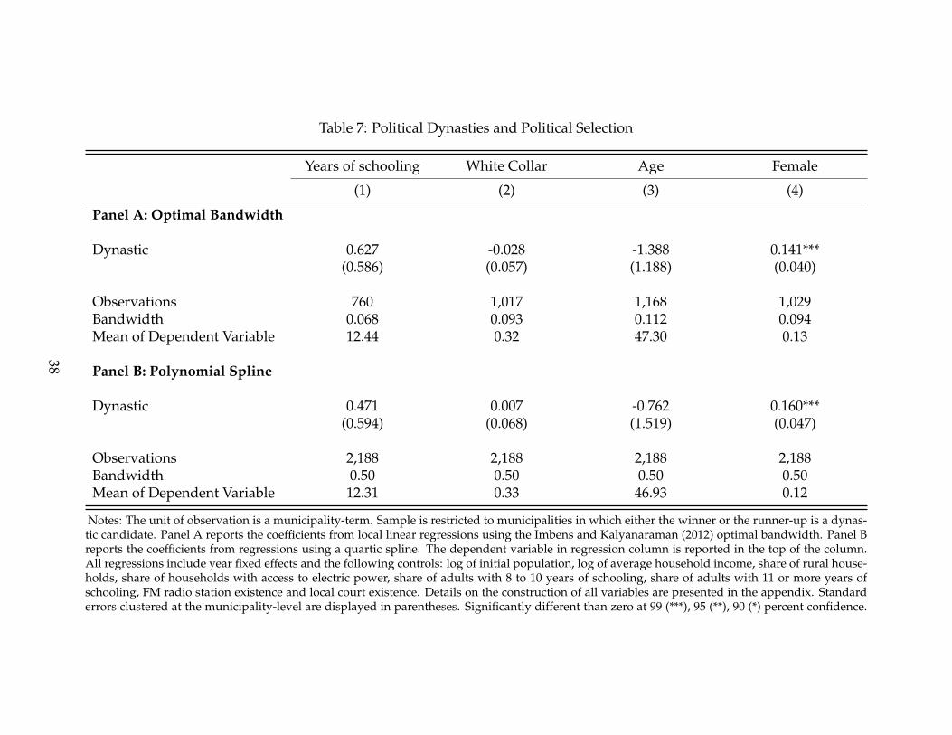
Table 7: Political Dynasties and Political Selection

Years of schooling White Collar Age Female

(1) (2) (3) (4)


Dynastic 0.627 -0.028 -1.388 0.141***(0.586) (0.057) (1.188) (0.040)

Observations 760 1,017 1,168 1,029Bandwidth 0.068 0.093 0.112 0.094Mean of Dependent Variable 12.44 0.32 47.30 0.13


Dynastic 0.471 0.007 -0.762 0.160***(0.594) (0.068) (1.519) (0.047)

Observations 2,188 2,188 2,188 2,188Bandwidth 0.50 0.50 0.50 0.50Mean of Dependent Variable 12.31 0.33 46.93 0.12


38

A Appendices

A.1 Data Sources

The data used in the paper comes from a variety of sources. The data is at the level ofthe municipality-municipal mandate, the lowest government unit below a state in Brazil.This means that growth rates are computed as the ratio between the increase from thebeginning to the end of the following term and the value at the beginning of the term.Next, we describe the source of each variable used in the analysis.

Politician’s Characteristics: the Tribunal Superior Eleitoral (TSE) provides basic demo-graphic information on each candidate that ran in municipal elections since the 1996 elec-tions at www.tse.gov.br. We use this information to create the following municipal-termindicators: Relative in Office in the future - Indicator of whether a candidate in 1996 hasa relative (details in the main text) in office in the future in the same municipality wonthe election, Dynastic - Indicator of whether a candidate in the 2004 or 2008 elections hasa relative in office in the past in the same municipality won the election, Age - Mayor’sAge, Female - Indicator of a female mayor, High Occupation - Indicator of mayor with awhite collar job , Schooling - Mayor’s years of schooling, Council Support - Councilors inthe government coalition/Number of Councilors, Campaign Contributions - Mayor’s cam-paign contribution.

Municipal demographic characteristics: Demographic characteristics of the municipalitycome from the 1992, 2000 and 2010 population census and the Contas Nacionais database,available at IBGE (www.ibge. gov.br). The estimate for the population in year of thesample was obtained from the IBGE inter-census population estimates. The variables usedin the analysis are: Literacy Rate - Proportion of the municipal population that is literate,Log of average household income - log(Average Household Income), Share of rural households -Proportion of the Municipal Population living in rural areas, Share of households with accessto eletric power - Proportion of the Municipal Population with Access to Eletric Power,Share of adults with 8 to 10 years of scholing - Proportion of the Municipal Population thatcompleted Middle School, Share of adults with 11 years or more of scholing - Proportion of theMunicipal Population that completed High School, Paved Roads (%) - Share of householdslocated in streets with paved roads, Open Sewage (%) - Share of households located insreeets with open sewage, Garbage in the Street (%) - Share of households located in sreeetswith garbage disposed.

Municipal institutional and public management characteristics: the 1999, 2002, 2005,

39

2006, 2008, 2009, 2011 and 2012 surveys of the Perfil dos Municípios Brasileiros: Gestão Pub-líca provide information on various aspects of the public administration and structuralmunicipal features. We constract the following variables from this source: AM Radio Sta-tion Existence - Existence of an AM Radio Station in the municipality, FM Radio StationExistence - Existence of an FM Radio Station in the municipality, Local Courts - Existenceof a Local Court in the Municiality, Public Emp. per 1000 inhabitants - 1000 * Employmentin Municipal Government / Population, Public Emp. per 1000 inhabitants (Permanent Staff)- 1000 * Employment in Municipal Government (Permanent Staff) / Population, PublicEmp. per 1000 inhabitants (Temporary Staff) - 1000 * Employment in Municipal Government(Temporary Staff) / Population.

Municipal public finance information: the National Treasury (Secretaria do Tesouro)provides information of spending and revenues through the FINBRA dataset. It con-tains municipal spending by categories. See www.tesouro.com.br. From this source, weconstruct all the outcomes in logs per capita so that log(Category Name pc) refers to log(Municipal Government Expenditures in this Category / Municipal Population). We con-sider the following categories cateegories Expenditures - total expenditures, Administrationand Planning, Education and Culture, Health and Sanitation, Social Assistance, Housing andUrban Development, Transportation - these 7 categories correspond to the break down of ex-penditure by function, Capital, Investment, Current - these last 3 categories correspond tothe break down of expenditure by the nature of the spending.

Private sector wages: the RAIS provides information of public and private sector workersand establishments for all (formal) firms in Brazil. We use this data to construct:Number ofworkers and Number of Establishments.

School data: information on the schools characteristics and enrollment came from yearlyschool census undertaken by INEP, while students’ performance came from Prova Brasil.We used here: Class Size - Average Class Size for 5th Graders Municipal Schools, InadequateAge - (Enrollment in Inadequate Grade for the Age) / (Total Enrollment) (5th Grade -Municipal Schools), Test Score - Average Test Score for 5th Graders in Municipal Schools(Math and Portuguese).

Health data: information on health outcomes was obtained from the Informações deSaúde (TABNET) available at www.datasus.gov.br. These include: 7+ Prenatal Visits -Share of women who had at least 7 prenatal visits, Share LBW - Share of low weight births,Infant Mortality - Number of Infant Deaths / Number of Births.

40

A.2 Additional Results

41

Table A1: Balance Tests

log(Population) % RuralHouse-holds

log(Avg.Income)

% ElectricPower

% HighSchool

% MiddleSchool

FM RadioStation

LocalCourt

(1) (2) (3) (4) (5) (6) (7) (8)


Dynastic 0.143 -0.033 -0.033 -0.013 -0.001 0.001 -0.035 -0.001(0.103) (0.029) (0.061) (0.017) (0.008) (0.005) (0.057) (0.067)

Observations 1,242 890 983 1,433 885 810 1,084 916Bandwidth 0.119 0.081 0.090 0.148 0.080 0.073 0.101 0.083Mean of Dependent Variable 9.31 0.43 6.81 0.83 0.13 0.10 0.33 0.48


Dynastic 0.068 -0.026 -0.036 -0.027 -0.006 -0.003 -0.046 -0.051(0.136) (0.032) (0.073) (0.024) (0.009) (0.006) (0.071) (0.075)

Observations 2,188 2,188 2,188 2,188 2,188 2,188 2,188 2,188Bandwidth 0.50 0.50 0.50 0.50 0.50 0.50 0.50 0.50Mean of Dependent Variable 9.31 0.43 6.84 0.83 0.13 0.10 0.34 0.47

Notes: The unit of observation is a municipality-term. Sample is restricted to municipalities in which either the winner or therunner-up is a dynastic candidate. Panel A reports the coefficients from local linear regressions using the Imbens and Kalya-naraman (2012) optimal bandwidth. Panel B reports the coefficients from regressions using a quartic spline. All regressions in-clude year fixed effects. Details on the construction of all variables are presented in the appendix. Standard errors clustered atthe municipality-level are displayed in parentheses. Significantly different than zero at 99 (***), 95 (**), 90 (*) percent confidence.

42

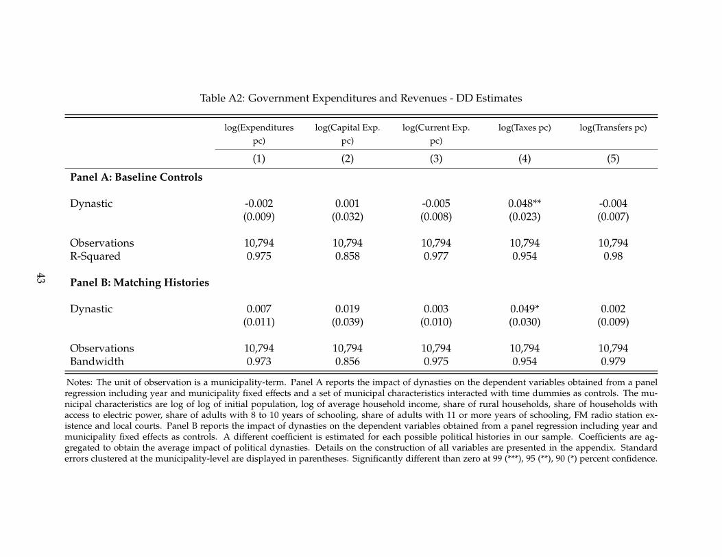
Table A2: Government Expenditures and Revenues - DD Estimates

log(Expenditurespc)

log(Capital Exp.pc)

log(Current Exp.pc)


(1) (2) (3) (4) (5)

Panel A: Baseline Controls

Dynastic -0.002 0.001 -0.005 0.048** -0.004(0.009) (0.032) (0.008) (0.023) (0.007)

Observations 10,794 10,794 10,794 10,794 10,794R-Squared 0.975 0.858 0.977 0.954 0.98

Panel B: Matching Histories

Dynastic 0.007 0.019 0.003 0.049* 0.002(0.011) (0.039) (0.010) (0.030) (0.009)

Observations 10,794 10,794 10,794 10,794 10,794Bandwidth 0.973 0.856 0.975 0.954 0.979

Notes: The unit of observation is a municipality-term. Panel A reports the impact of dynasties on the dependent variables obtained from a panelregression including year and municipality fixed effects and a set of municipal characteristics interacted with time dummies as controls. The mu-nicipal characteristics are log of log of initial population, log of average household income, share of rural households, share of households withaccess to electric power, share of adults with 8 to 10 years of schooling, share of adults with 11 or more years of schooling, FM radio station ex-istence and local courts. Panel B reports the impact of dynasties on the dependent variables obtained from a panel regression including year andmunicipality fixed effects as controls. A different coefficient is estimated for each possible political histories in our sample. Coefficients are ag-gregated to obtain the average impact of political dynasties. Details on the construction of all variables are presented in the appendix. Standarderrors clustered at the municipality-level are displayed in parentheses. Significantly different than zero at 99 (***), 95 (**), 90 (*) percent confidence.

43

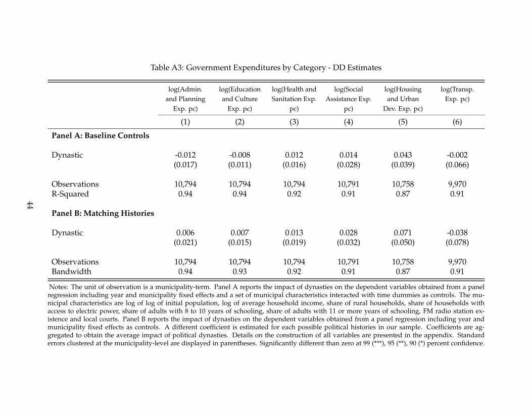
Table A3: Government Expenditures by Category - DD Estimates

log(Admin.and Planning

Exp. pc)

log(Educationand Culture

Exp. pc)


pc)

log(SocialAssistance Exp.

pc)

log(Housingand Urban

Dev. Exp. pc)

log(Transp.Exp. pc)

(1) (2) (3) (4) (5) (6)


Dynastic -0.012 -0.008 0.012 0.014 0.043 -0.002(0.017) (0.011) (0.016) (0.028) (0.039) (0.066)

Observations 10,794 10,794 10,794 10,791 10,758 9,970R-Squared 0.94 0.94 0.92 0.91 0.87 0.91


Dynastic 0.006 0.007 0.013 0.028 0.071 -0.038(0.021) (0.015) (0.019) (0.032) (0.050) (0.078)

Observations 10,794 10,794 10,794 10,791 10,758 9,970Bandwidth 0.94 0.93 0.92 0.91 0.87 0.91


44

Table A4: Economic Performance - DD Estimates

GDP Growth AgriculturalGDP Growth

ManufacturingGDP Growth

Services GDPGrowth

No. ofEmployees

Growth

No. ofEstablishments

Growth

(1) (2) (3) (4) (5) (6)


Dynastic 0.029 0.022 0.060 0.014 0.102 -0.012(0.020) (0.040) (0.076) (0.015) (0.179) (0.028)



Dynastic 0.041 -0.036 0.176 0.024 0.272 0.019(0.028) (0.058) (0.126) (0.024) (0.272) (0.019)



45

Table A5: Quality of Public Goods - DD Estimates

Education Health

Class Size InadequateAge

Test Score 7+ PrenatalVisits

Low BirthWeight

InfantMortality

(1) (2) (3) (4) (5) (6)


Dynastic 0.165 0.001 -0.033 0.003 0.001 0.163(0.270) (0.006) (0.047) (0.007) (0.001) (0.595)



Dynastic 0.388 -0.014 -0.046 0.009 0.002 0.108(0.369) (0.009) (0.054) (0.009) (0.002) (0.777)



46

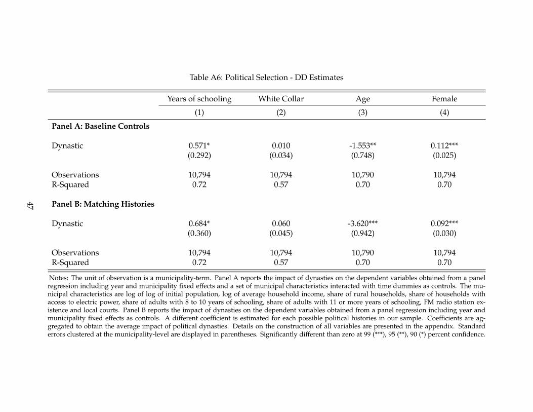
Table A6: Political Selection - DD Estimates

Years of schooling White Collar Age Female

(1) (2) (3) (4)


Dynastic 0.571* 0.010 -1.553** 0.112***(0.292) (0.034) (0.748) (0.025)

Observations 10,794 10,794 10,790 10,794R-Squared 0.72 0.57 0.70 0.70


Dynastic 0.684* 0.060 -3.620*** 0.092***(0.360) (0.045) (0.942) (0.030)

Observations 10,794 10,794 10,790 10,794R-Squared 0.72 0.57 0.70 0.70


47

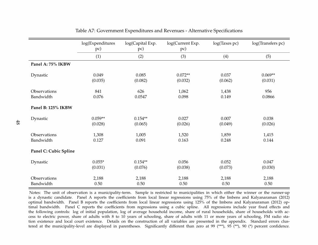
Table A7: Government Expenditures and Revenues - Alternative Specifications

log(Expenditurespc)

log(Capital Exp.pc)

log(Current Exp.pc)


(1) (2) (3) (4) (5)

Panel A: 75% IKBW

Dynastic 0.049 0.085 0.072** 0.037 0.069**(0.035) (0.082) (0.032) (0.062) (0.031)

Observations 841 626 1,062 1,438 956Bandwidth 0.076 0.0547 0.098 0.149 0.0866

Panel B: 125% IKBW

Dynastic 0.059** 0.154** 0.027 0.007 0.038(0.028) (0.065) (0.026) (0.049) (0.026)


Panel C: Cubic Spline

Dynastic 0.055* 0.154** 0.056 0.052 0.047(0.031) (0.076) (0.038) (0.073) (0.030)


Notes: The unit of observation is a municipality-term. Sample is restricted to municipalities in which either the winner or the runner-upis a dynastic candidate. Panel A reports the coefficients from local linear regressions using 75% of the Imbens and Kalyanaraman (2012)optimal bandwidth. Panel B reports the coefficients from local linear regressions using 125% of the Imbens and Kalyanaraman (2012) op-timal bandwidth. Panel C reports the coefficients from regressions using a cubic spline. All regressions include year fixed effects andthe following controls: log of initial population, log of average household income, share of rural households, share of households with ac-cess to electric power, share of adults with 8 to 10 years of schooling, share of adults with 11 or more years of schooling, FM radio sta-tion existence and local court existence. Details on the construction of all variables are presented in the appendix. Standard errors clus-tered at the municipality-level are displayed in parentheses. Significantly different than zero at 99 (***), 95 (**), 90 (*) percent confidence.

48

Table A8: Expenditures by Category - Alternative Specifications

log(Admin. andPlanning Exp.

pc)

log(Educationand Culture Exp.

pc)


pc)

log(SocialAssistance Exp.

pc)

log(Housing andUrban Dev. Exp.

pc)

log(Transp. Exp.pc)

(1) (2) (3) (4) (5) (6)

Panel A: 75% IKBW

Dynastic 0.043 0.005 0.079 0.108 0.293** 0.527*(0.053) (0.041) (0.050) (0.080) (0.133) (0.286)

Observations 1,068 794 727 1,009 628 440Bandwidth 0.099 0.071 0.065 0.092 0.055 0.043

Panel B: 125% IKBW

Dynastic 0.014 0.032 0.115*** 0.008 0.364*** 0.637***(0.043) (0.033) (0.040) (0.063) (0.106) (0.213)

Observations 1,531 1,240 1,141 1,465 1,012 735Bandwidth 0.165 0.119 0.108 0.153 0.092 0.071


Dynastic 0.062 0.033 0.081** 0.052 0.196* 0.347*(0.053) (0.036) (0.041) (0.076) (0.100) (0.178)



49

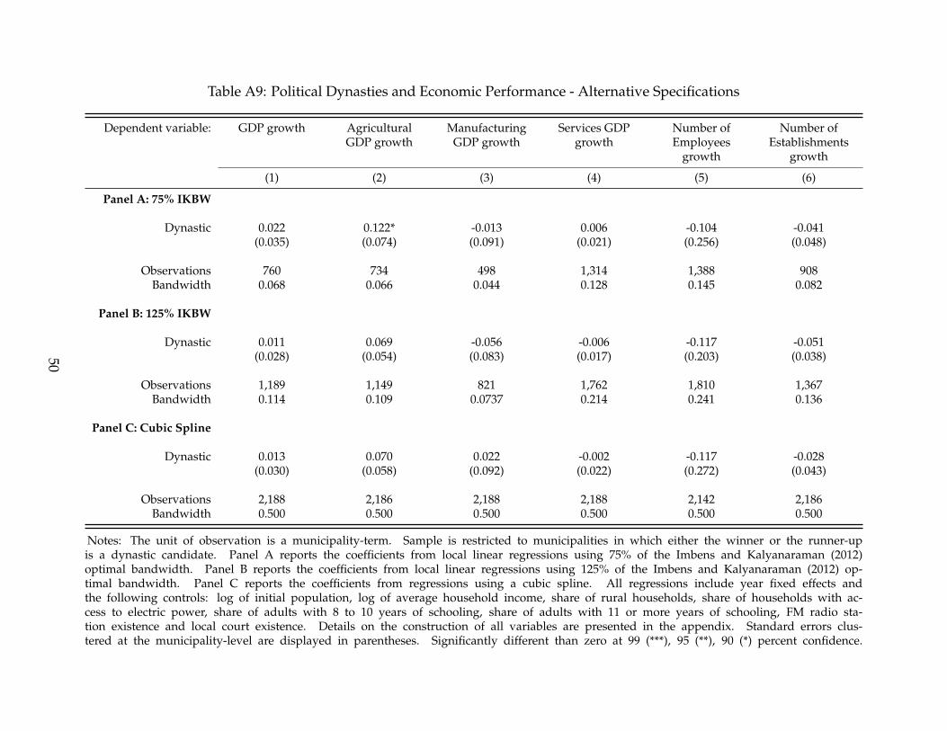
Table A9: Political Dynasties and Economic Performance - Alternative Specifications

Dependent variable: GDP growth AgriculturalGDP growth

ManufacturingGDP growth

Services GDPgrowth

Number ofEmployees

growth

Number ofEstablishments

growth

(1) (2) (3) (4) (5) (6)

Panel A: 75% IKBW

Dynastic 0.022 0.122* -0.013 0.006 -0.104 -0.041(0.035) (0.074) (0.091) (0.021) (0.256) (0.048)

Observations 760 734 498 1,314 1,388 908Bandwidth 0.068 0.066 0.044 0.128 0.145 0.082

Panel B: 125% IKBW

Dynastic 0.011 0.069 -0.056 -0.006 -0.117 -0.051(0.028) (0.054) (0.083) (0.017) (0.203) (0.038)

Observations 1,189 1,149 821 1,762 1,810 1,367Bandwidth 0.114 0.109 0.0737 0.214 0.241 0.136


Dynastic 0.013 0.070 0.022 -0.002 -0.117 -0.028(0.030) (0.058) (0.092) (0.022) (0.272) (0.043)



50

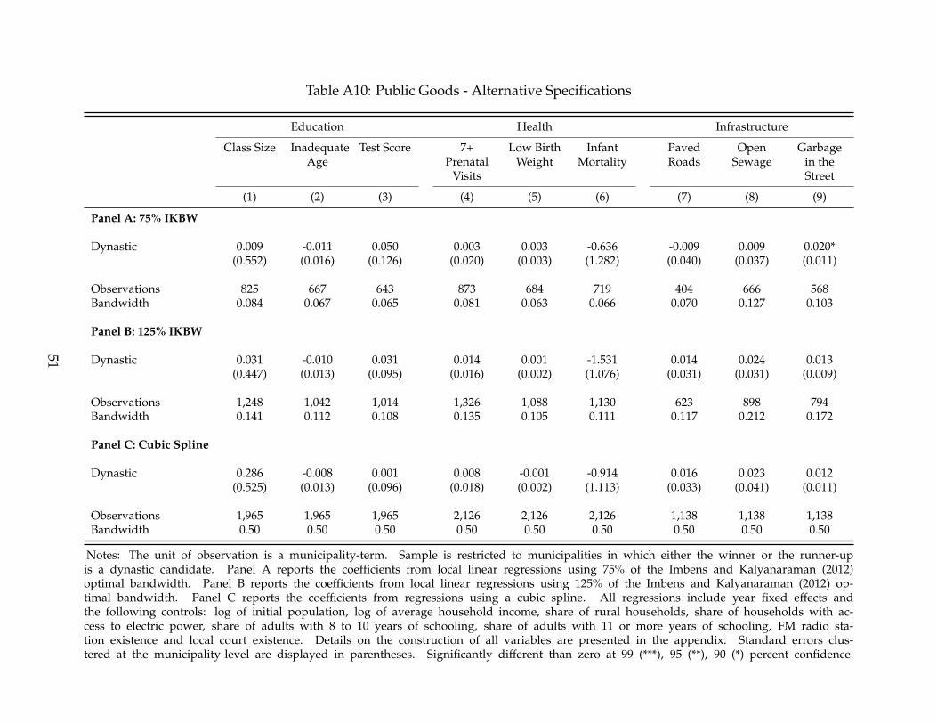
Table A10: Public Goods - Alternative Specifications

Education Health Infrastructure

Class Size InadequateAge

Test Score 7+Prenatal

Visits

Low BirthWeight

InfantMortality

PavedRoads

OpenSewage

Garbagein theStreet

(1) (2) (3) (4) (5) (6) (7) (8) (9)

Panel A: 75% IKBW

Dynastic 0.009 -0.011 0.050 0.003 0.003 -0.636 -0.009 0.009 0.020*(0.552) (0.016) (0.126) (0.020) (0.003) (1.282) (0.040) (0.037) (0.011)

Observations 825 667 643 873 684 719 404 666 568Bandwidth 0.084 0.067 0.065 0.081 0.063 0.066 0.070 0.127 0.103

Panel B: 125% IKBW

Dynastic 0.031 -0.010 0.031 0.014 0.001 -1.531 0.014 0.024 0.013(0.447) (0.013) (0.095) (0.016) (0.002) (1.076) (0.031) (0.031) (0.009)

Observations 1,248 1,042 1,014 1,326 1,088 1,130 623 898 794Bandwidth 0.141 0.112 0.108 0.135 0.105 0.111 0.117 0.212 0.172


Dynastic 0.286 -0.008 0.001 0.008 -0.001 -0.914 0.016 0.023 0.012(0.525) (0.013) (0.096) (0.018) (0.002) (1.113) (0.033) (0.041) (0.011)

Observations 1,965 1,965 1,965 2,126 2,126 2,126 1,138 1,138 1,138Bandwidth 0.50 0.50 0.50 0.50 0.50 0.50 0.50 0.50 0.50


51

Table A11: Political Dynasties and Political Selection - Alternative Specifications

Dependent Variable: Years of schooling White Collar Age Female

(1) (2) (3) (4)

Panel A: 75% IKBW

Dynastic 0.001 0.525 -1.565 0.120**(0.067) (0.679) (1.365) (0.046)

Observations 773 575 924 791Bandwidth 0.069 0.051 0.084 0.071

Panel B: 125% IKBW

Dynastic -0.005 0.465 -2.408** 0.128***(0.052) (0.530) (1.063) (0.037)

Observations 1,208 935 1,386 1,229Bandwidth 0.116 0.085 0.140 0.118


Dynastic 0.020 0.697 -2.196* 0.148***(0.056) (0.477) (1.227) (0.039)

Observations 2,188 2,188 2,188 2,188Bandwidth 0.50 0.50 0.50 0.50


52

Political Dynasties and the Quality of Government

Documents

Transcript of Political Dynasties and the Quality of Government