Political Corruption and Voter Turnout: Mobilization or ...
35
Political Corruption and Voter Turnout: Mobilization or Disaffection? Elena Costas-Pérez Universitat de Barcelona & Institut d’Economia de Barcelona (IEB) Work in progress. March 2014. ABSTRACT: Corruption scandals may modify voter turnout, either by mobilizing citizens to go to the polls to punish or support the malfeasant politician or by demotivating individuals to vote as a consequence of disaffection with the democratic process. We study whether these effects depend on individual’s partisan leanings and/or the timing of corruption scandals. Our database includes information on Spanish local scandals from 1999 to 2007, and survey data on individuals’ turnout at the 2007 local elections. We use a matched database to identify the corruption-free pairs for our corruption affected municipalities’ sample. Our results show that while neither past nor recent corruption scandals have impact on turnout, repeated corruption cases boost abstentionism. We also find that independent voters - those with no attachment to any political party - are the only ones that withdraw from elections as a consequence of corruption. Core supporters do not modify their electoral participation after a scandal has broken out. Those who support the incumbent do not even recognise that their party is corrupt, while both independent voters and opposition core supporters report higher levels of corruption perceptions once a scandal is revealed. Keywords: electoral turnout, accountability, corruption JEL Classification: P16, D72, D73 Contact address: Faculty of Economics and Business University of Barcelona Av. Diagonal 690, torre4, planta 2ona 08034 Barcelona Telf.: 00 34 93 403 90 12 e-mail: [email protected]
Transcript of Political Corruption and Voter Turnout: Mobilization or ...

Political Corruption and Voter Turnout:
Mobilization or Disaffection?
Elena Costas-Pérez
Universitat de Barcelona &
Institut d’Economia de Barcelona (IEB)
Work in progress. March 2014.
ABSTRACT: Corruption scandals may modify voter turnout, either by
mobilizing citizens to go to the polls to punish or support the malfeasant
politician or by demotivating individuals to vote as a consequence of
disaffection with the democratic process. We study whether these
effects depend on individual’s partisan leanings and/or the timing of
corruption scandals. Our database includes information on Spanish local
scandals from 1999 to 2007, and survey data on individuals’ turnout at
the 2007 local elections. We use a matched database to identify the
corruption-free pairs for our corruption affected municipalities’ sample.
Our results show that while neither past nor recent corruption scandals
have impact on turnout, repeated corruption cases boost abstentionism.
We also find that independent voters - those with no attachment to any
political party - are the only ones that withdraw from elections as a
consequence of corruption. Core supporters do not modify their
electoral participation after a scandal has broken out. Those who
support the incumbent do not even recognise that their party is corrupt,
while both independent voters and opposition core supporters report
higher levels of corruption perceptions once a scandal is revealed.
Keywords: electoral turnout, accountability, corruption
JEL Classification: P16, D72, D73
Contact address:
Faculty of Economics and Business
University of Barcelona
Av. Diagonal 690, torre4, planta 2ona
08034 Barcelona
Telf.: 00 34 93 403 90 12
e-mail: [email protected]

1
1. Introduction
In democratic systems elections are an instrument through which citizens can punish
dishonest politicians by not voting for them, bringing down corrupt governments.
Studies on the effect of scandals on electoral outcomes do not find vast electoral
punishments of corruption, implying that in most cases malfeasant politicians are re-
elected1. These results have sometimes been interpreted as cultural acceptance of
corruption, a hypothesis that considers some societies more tolerant of scandals, as
voters do not react to them.
Nevertheless, it is important to remember that electoral outcomes are the result of who
votes and for whom. Once an election is called, individuals face the choice of a
participation decision. Some citizens may react to corruption by changing their decision
of whether to vote or abstain, rather than by withholding their electoral support for the
accused incumbent. In such cases, scandals would affect electoral outcomes in a broader
way than the incumbent’s vote share. To properly identify the overall impact of the
effect of corruption, voter turnout must be also considered.
Corruption scandals may modify individuals’ participation decision, either by
mobilizing people to go to the polls to punish or support the malfeasant politician or by
demotivating them to vote as a consequence of disaffection with the democratic process.
We refer to the former as a “mobilization effect” and to the latter as a “disaffection
effect” of corruption. Most of the studies focus on the aggregated impact of scandals on
voter turnout without distinguishing between the mobilization and disaffection effects
that corruption may have on individual electoral participation (Dominguez and McCann
and, 1998). Existing literature presents ad hoc explanations of turnout variations, which
do not respond to a planned strategy to identify those different effects. Hence, once the
analysis is done the impact of either the mobilization or the disaffection effects cannot
be differentiated. Moreover, aggregate level data used in some studies (i.e., Stockemer,
2013, or Stockemer et al., 2013) represents an additional obstacle to determining the
relative power of corruption’s mobilization and disaffection effects.
The aim of this paper is to analyse whether individuals modify their participation in
local elections after a corruption scandal affecting the incumbent is revealed. Using data
at the individual level, we are able to identify the mobilization and disaffection effects
that corruption may generate considering both the individual’s partisan leanings and the
timing of the scandals.
1Peters and Welch (1980); Welch and Hibbing (1997); Jiménez and Caínzos (2003); Ferraz and Finan
(2008); Rivero and Fernandez-Vazquez (2010); Chong, et al. (2012); Costas-Pérez, et al. (2012);
Fernández-Vázquez et al. (2013); and Winters and Weitz-Shapiro (2013).

2
On one hand, depending on partisan leanings, some citizens could be more or less likely
to be mobilized to vote as a result of corruption scandals. Individuals with strong
political leanings tend to go to the ballot to support their politicians. Also, higher
degrees of partisanship are a factor that may influence some individuals’ evaluation of
corruption scandals (Rundquist et al., 1977; Anduiza et al., 2012). In contrast,
individuals who occasionally vote do not exhibit high partisan attachments and are
likely to be more sensitive to scandals (Chong et al., 2012). Thus, the degree of
partisanship will play a crucial role in determining how citizens perceive accusations of
corruption of the incumbent, and how they translate their perceptions into voter
behaviour.
On the other hand, scandals occurring at different times may affect participation
decisions differently. Recent corruption cases may mobilize voters to the polls, while
past scandals may be forgotten (Fair 1978; Kramer 1971). Moreover, the timing of
corruption cases may also be a key issue shaping faith in the democratic system.
Repeated corruption cases might generate disaffection with the electoral system among
politically alienated citizens who eventually withdraw from participation in elections
(Kostadinova, 2009).
We consider local corruption scandals in Spain, which constitutes a good scenario for
use in testing the effects that corruption may have on electoral outcomes. The Spanish
case combines a recent wave of local scandals concentrates on the 2003 to 2007 term of
office, with a significant number of municipalities that have experienced repeated
corruption cases in two consecutive terms of office (1999 to 2003 and 2003 to 2007).
Our database on local corruption scandals allow us to verify if past, recent or repeated
corruption cases lead to different effects on voter turnout. Additionally to this database
we benefit from a survey run in several Spanish municipalities affected and non affected
by corruption scandals, recollecting individual information on, among others, voting
behaviour in the 2007 local elections, degree of partisanship, ideology, and corruption
perceptions2. The use of that specific survey data at the individual level permits us to
analyse the mobilization and disaffection effect of corruption on turnout depending on
the voter’s partisan leanings.
The matching strategy allows the identification of a valid control group for the
municipalities affected by corruption. A part from selecting the twin municipalities that
did not experience scandals in the period analysed, matching methods provides with
further advantages. First, the use of a matched sample improves the identification of the
2 We make use of both a matching sample and a survey designed by Solé-Ollé, A. and Sorribas-Navarro,
P. for the study “Does Exposure to Corruption Erode Trust in Government? Evidence from a Matched
Sample of Local Scandals in Spain” presented at the 7th Workshop on Political Economy (November
2013, Dresden).
3
effect of corruption scandals on voter turnout, balancing the distribution of the
covariates of the two subsamples. Matching also increases the transparency of our
research design, as described in more detail in the section 3.2. We also report a series of
placebo tests that confirm the validity of our identification strategy.
Our results show that, on average, local corruption scandals make citizens 2.1% less
likely to vote. However, not all individuals modify in the same way their electoral
participation as a consequence of corruption. This study shows that partisan leanings
play a key role on shaping individuals’ response to corruption. We find that independent
voters are 3.6% less likely to vote if a corruption scandal occurs in their municipalities.
Core supporters, defined as those citizens who always vote for the same party, do not
seem to react to corruption scandals, irrespective of whether they support the incumbent
party or the opposition.
Regarding the timing of corruption scandals, we find that it is just when corruption is
repeated in different periods that citizens decide to abstain, disappearing that effect for
cases occurring either far away in time or in the years previous to the election analysed.
Analysing both individual’s partisan leanings and the timing of corruption, our results
show that corruption just has an effect on independent voters. We find that these
individuals are less likely to vote also in municipalities that have experienced past or
repeated corruption cases, accounting the later a 5.4% decrease in their likelihood of
voting. That implies that the disaffection effect of scandals predominates over the
mobilization factor.
Measuring the effect of scandals on voters’ corruption perceptions we can observe that
independent voters report higher levels of corruption perceptions after a scandal is
revealed. Core supporters of the incumbent involved in a corruption scandal do not
seem to realise that corruption occurs. On the contrary, core supporters of the opposition
parties increase their corruption perceptions if a scandal is revealed. We also find that in
the short term local scandals do affect corruption perceptions, but that does not modify
immediately individuals’ participation decision.
We make three main contributions to the existing literature. First, we benefit from a
research strategy specifically designed to distinguish between the mobilization and
disaffection effects of corruption on voter turnout. Second, this is the first paper to our
knowledge that empirically analyses how these two effects depend on partisan leanings.
We are able to identify the individuals who are potentially mobilized to vote, and those
who withdraw from elections as a consequence of corruption scandals. Third, we
contribute to the literature by testing the impact of corruption occurring at different
times on voter turnout, allowing us to untangle conclusions from earlier investigations
that did not differentiate voter’ responses based on the timing of scandals.

4
Additionally, our study provides empirical evidence on the effect of actual corruption
cases. Most of the empirical papers on corruption’s determinants and consequences rely
on perceptions, which are easier to obtain but raise concerns on both their bias and their
accuracy with corruption itself. Moreover, we do not consider corruption at the
aggregate level, if not local corruption cases. Measuring corruption at the municipal
level provide us with a more extensive sample of cases. It also has an additional
advantage, since local cases makes easier for citizens to link each scandal with the
corresponding local politician, potentially increasing the accountability of municipal
elections.
The rest of the paper is organized as follows. The next section provides the reasons that
the timing of corruption and partisan leanings could affect turnout once a scandal is
revealed, and outlines the main hypothesis to test. Section 3 defines the empirical
analysis followed and the construction of the database. Section 4 discusses the
estimation strategy. Section 5 presents the results and, lastly, section 6 concludes.
2. Corruption’s mobilization and disaffection effects
2.1. Previous literature
Neither theoretical nor empirical studies have arrived at unified conclusions on the
relationship between corruption and voter turnout3. An important shortcoming of
existing literature is the lack of an empirical strategy designed to identify the effects
once a scandal breaks out, i.e., an increase in electoral participation through a
mobilization of voters to the polls or a decrease of electoral participation as a result of
their disaffection with the democratic process. Kostadinova’s (2009) study on post-
communist transitional countries tries to identify both a direct –mobilization- and an
indirect –disaffection- effect of corruption on turnout. However, she considers
corruption perceptions, which may be correlated to voting decisions, casting doubt on
the model’s overall exogeneity.
It has been proven that good governance is related to citizens’ capacity to hold their
politicians accountable (Adsera, et al., 2003). Hence, if we understand elections as an
effective accountability tool, individuals who feel betrayed by a corrupt politician may
cast a ballot to bring him or her out of power. In such a case, corruption would act as a
mobilization factor. That mobilization effect would make some citizens, who would
otherwise abstain, go to the polls to punish the accused politician. After a scandal, party
3 In most cases empirical evidence confirms a negative relationship between corruption and turnout
(Domínguez and McCann, 1998; Kostadinova, 2009; Birch, 2010; Chong et al., 2012). In contrast, a
scholarly minority (Karahan et al., 2006; Escaleras et al., 2012) attributes to corruption a positive effect
on turnout. Finally, some studies do not find any relationship between corruption scandals and voter
turnout (Stockemer, 2013).

5
members and sympathisers could also be called upon to mobilize to give their vote to
the accused politician, either by thinking the allegations are false or by giving
unconditional support. An alternative case, in the context of highly corrupt situations
with clientelistic networks, is that scandals could stimulate turnout if corrupt politicians
were to buy voters to retain their power (Karahan et al., 2006).
Conversely, corruption can also be a drain on voter turnout (Putnam, 1993; Warren,
2004; Chang and Chu, 2006). Corruption harms citizens’ trust in local and national
politicians, generating cynicism and voter apathy (Solé-Ollé and Sorribas-Navarro,
2013). That disaffection effect would make individuals less likely to vote for existing
corrupt political parties (Warren, 2004; Wagner et al., 2009). If corruption is repeated,
in the long run disaffected individuals may decide to disengage from the electoral
system (Chong et al., 2012). If voters consider that corruption is widespread, replacing
the corrupt incumbent for a new one will not fix the situation. In the most extreme
cases, widespread corruption might also cast doubt on the sustainability of the
democratic system (Kostadinova, 2009). Empirical evidence has confirmed this
negative relationship between corruption and turnout (Domínguez and McCann, 1998;
Andersen and Tverdova, 2003; Kostadinova, 2009; Stockemer, 2013; and Stockemer et
al., 2013).
2.2. Who and why will be affected by corruption?
As stated above, most existing studies are unable to differentiate among the relative
strengths of the mobilization and disaffection effects that actual corruption cases may
cause. We argue that the literature on corruption and voter turnout does not point
conclusively to voters’ reactions because two crucial factors are excluded from these
analyses: the role of individual partisan leanings and the timing of corruption.
First, we consider that corruption’s mobilization and disaffection effects will differ
depending on voters’ degree of partisan affinity with the incumbent involved. Similar to
our strategy, Chong et al. (2012) take a step forward over previous studies, proving with
experimental evidence for Mexico that exposing citizens to information on corruption
not only decreases voter turnout, but also negatively affects voters’ identification with
the corrupt incumbent's party. They find that providing information about high levels of
corruption has a bigger impact on challengers' votes than on incumbents'; however, their
data does not allow them to analyse if voters with a different degree of partisanship
respond differently to corruption.
Independent voters, those who occasionally vote or do not always vote for the same
party, tend to be more independent from partisan attachments, and they can be more
affected by shocks like occasional corruption (Rundquist et al., 1977; Feddersen and
Pesendorfer, 1996; Sobbrio and Navarra, 2010; Stockemer, 2013). Thus, the

6
disaffection effect will be higher for those, so we would expect to observe independent
voters withdrawing from the elections if corruption scandals occur. Hence, the first
hypothesis regarding partisan leaning is:
H1.a: Independent voters, defined as those who do not always vote for the same party,
will be more likely to abstain if a corruption scandal is revealed.
On the contrary, core supporters have stronger partisan leanings and are less likely to
defect (Chong et al., 2012). If partisan leanings are strong, citizens may disregard
corruption as a determining factor in their decision and continue to vote for the party to
which they are ideologically aligned (Peters and Welch, 1980; and Anderson and
Tverdova, 2003). Ideology or party identification can also modify how voters evaluate
corruption, depending on the party to which the corrupt incumbent belongs. Supporting
this hypothesis, recent research of Anduiza et al. (2012) finds that individuals have a
partisan bias and are more tolerant to corruption if the politician involved belongs to
their own party. If that is true, we should find core supporters of corrupt incumbents
unaffected by corruption scandals when deciding to vote. Thus, the hypothesis to test is:
H1.b: Incumbent core supporters will not modify their electoral participation decision
after an incumbent’s corruption scandal is revealed.
Considering core supporters of opposition parties, we would expect that, even realising
that corruption exists, they will keep voting for their party options. It may be even
possible that, in the presence of corruption, some opposition core supporters who would
otherwise abstain would go to the polls to defeat the corrupt incumbent. Nevertheless,
people who identify themselves with a political party are more likely to vote (Norris,
2004), so it is improbable that we will find that mobilization effect. Regarding partisan
leanings, the last hypothesis is:
H1.c: Opposition core supporters will not modify their electoral participation decision
after an incumbent’s corruption scandal is revealed.
Second, we consider that scandals occurring at different points in time may modify the
influence of corruption’s mobilization or disaffection effect on individual participation
decision. There is evidence that voters tend to overweigh the information received
closer to elections, as recent events have greater influence on evaluations of
incumbents’ performance (Fair 1978; Kramer 1971). Another explanation for the fact
that later scandals could have greater effects on turnout is that voters are more attentive
to indicators of incumbents’ outcomes as an election approaches (Valentino and Sears
1998), being unable to easily recollect information on earlier performance (i.e., past

7
corruption cases) (Huber et al. 2012). Also, old corruption cases might be difficult for
voters to remember.
Thus, while in the short term corruption can mobilize voters to bring down corrupt
governments, that relationship can be reversed if corruption continues over time. This
hypothesis is based on the fact that the persistence of corruption can differently affect
citizens’ trust in the political system. Corruption cases repeated over several years can
make citizens cast doubt on the democratic system’s capacity to keep politicians
accountable (Kostadinova, 2009). That distrust in the political system leads to
disaffection and alienation from politics, which may result in the decision to withdraw
from the electoral process, i.e., abstention. In that scenario, repeated corruption cases
will then generate the disaffection mechanism through which corruption scandals lessen
voter turnout.
Hence, the hypothesis regarding the effects of the timing of corruption cases on voters’
turnout is:
H2: Past corruption cases will not affect turnout, while recent scandals would either
have no effect or would mobilize people to vote. Repeated corruption in time will lessen
voter turnout as a result of the disaffection effect.
In conducting our study, we analyse these hypotheses, both independently and
considered together. We predict that independent voters - those more susceptible to
defection - will be more sensitive to repeated corruption scandals, which will further
harm their trust in the system. Regarding core supporters, it is difficult to speculate how
they will react to corruption occurring at different times, since we predict that they will
be less likely to modify their electoral participation as a consequence of corruption.
3. Data and Empirical Analysis
3.1. Data and typology of corruption scandals
In order to carry out our analysis, we use a novel database that includes information on
local corruption scandals in Spain and data on a survey of voting behaviour in Spanish
municipalities. We define a local corruption scandal as the “public allegation of
corruption brought to light by a newspaper”. Our data about corruption cases is based
on a report compiled by the Fundación Alternativas (2007). After a wave of local
corruption scandals starting in the first years of the 2000s, that Spanish think-tank hired
several journalists to gather all corruption-related stories published in national, regional
and local media between January 2000 and January 2007. However, the time period we
are interested in goes from the local elections in July 1999 to the ones in May 2007. For
that reason, we completed the Fundación Alternativas’s information with an internet-

8
guided search4 on news on corruption scandals. We ended up with a total of 565
municipalities affected by corruption scandals during that period5. We also checked for
the non-partisan bias of our news, comparing our data with other corruption maps
compiled by media outlets from different political ideologies. The percentage of
corruption cases by political party was not statistically different in all databases,
verifying that our compilation of cases was not ideologically biased.
It is important to bear in mind that during the first Spanish democratic governments
(1979-1999) there were no exceedingly significant local corruption cases reflected in
Spanish media (Jiménez and Caínzos, 2006). The corruption cases we are studying are
related to land use regulations, one of the most important local corruption’s typologies
in Spain during the peak of the housing boom. Scandals involved local politicians
receiving bribes in return to changes over the land use plans already approved (i.e.,
reclassifying public land). Municipal governments in Spain are responsible for the land
use regulation, making easier to identify the effect of those scandals on electoral
outcomes. In that specific case, voters can clearly identify the incumbent as guilty for
the land-use related corruption.
The wave of corruption cases rose significantly in the late nineties, when Spanish media
started highlighting numerous corruption scandals and the judiciary also began the
investigation of some of them. The number of corruption cases shot up after 1999
(Costas-Pérez et al., 2012), peaking before the 2007 local elections. That distribution of
scandals makes the Spanish situation the optimal context to test our hypothesis that
corruption occurring at different points in time will have a different effect on citizens’
voting behaviour.
Our database accounts for 122 municipalities affected by corruption in the period from
June 1999 to May 2007. We have classified them among three different sub-categories
regarding corruption persistence that we will use throughout our analysis. First, 32
municipalities of our database experienced at least one corruption scandal in the term
1999-2003, but not corruption cases broke out afterwards. We have considered them as
‘past corruption cases’, since in the 2007 elections voters may have a faint memory
about these scandals. Second, 58 municipalities had at least one corruption scandal in
the term 2003-2007, but not corruption cases had broke out in the previous term. These
are classified as ‘recent corruption cases’ from the perspective of an individual facing
the 2007 local election. Finally, we have also considered those places that have
4 We used a paid digital information management service covering all national and many of the regional
newspapers, MyNews, until November 2009. Thus, we have an additional sample of corruption cases
occurring between the local elections of 2007 and November 2009 that we save to perform a placebo test
explained in section 4.6. 5 See Costas-Pérez et al. (2012) for more information on the construction of the corruption database.

9
experience repeated corruption cases, both in the 1999-2003 and the 2003-2007 terms.
32 municipalities are classified in the category of ’repeated corruption cases’.
Hence, our corruption database indicates whether there has been at least one corruption
scandal between June 1999 and May 2007 (the two terms of office analysed). Since our
objective is to measure the impact of corruption, we need a sample of individuals from
corruption-free municipalities to be compared with those from localities affected by
scandals. The fact of using a matched set of municipalities allows us to balance the
distribution of covariates between corruption-ridden and corruption-free municipalities,
to avoid biased estimations.
3.2. The matching strategy
In order to construct our analysis’ sample we use a matched database that identifies for
the selected municipalities affected by corruption a valid control group. Budget
limitations implied a restriction for the number of municipalities analysed in the survey.
Hence, a matching procedure was followed to select those corruption-free
municipalities to be compared with the corruption-ridden ones (our control and
treatment groups, respectively). Over the 565 municipalities that experienced at least
one corruption scandal between 1999 and 2007, a sample of 122 municipalities was
randomly select – stratified according to population size and term of corruption -. Thus,
old and new corruption cases are equally represented in the final database.
The municipalities that potentially belong to the control group are those with similar
characteristics to the corruption-ridden ones but where no scandals broke out. In order
to identify our control group a Propensity Score Matching approach was used6.
In order to construct the ‘propensity score’ a Logit model7 was estimated, using as a
dependent variable a dummy equal to one if a corruption scandal broke out in the
municipality, and zero otherwise. The Logit equation was estimated with data from all
the corruption-ridden and corruption-free municipalities. The municipal-level variables
used to implement the matching strategy were8: historical average levels of aggregate
turnout, population size, unemployment, ethnic diversity, income, school attendance,
divorce rate, and historical average of right voters9.
6 The full procedure and estimations results of Solé-Ollé and Sorribas-Navarro’s (2013) matching
strategy, as well as additional data checks, are available upon request. 7 Because of data limitations to carry out the matching we were limited to municipalities larger than 1.000
habitants. 8 Descriptive statistics of these data can be found in Table A.1. in the Appendix.
9 Two alternative estimations were also considered, including some additional covariates with low
explanatory power (i.e., percentage of elderly population, historical average of electoral margin of
victory, coalition governments, percentage of residents born in that municipality, newspapers per capita
or associations per capita), and also higher order terms of the main covariates and interactions amongst
them. Nevertheless, the balance did not improve in either case, so the first option was maintained.

10
With the Logit estimation the ‘propensity score’ was computed and control
municipalities were matched to the treatment ones based on having a similar value of
the ‘propensity score’. As the matching algorithm the ‘Nearest Neighbour with
replacement’10
was use. This method allows for more than one given control unit
matching more than one treatment unit, which increases the average quality of matching
and reduces the bias11
.
The matching strategy’s implementation allows to balance the covariates in the two
subsamples. We ended up with a control group of 97 municipalities that did not
experience any corruption scandal between 1999 and 2007. These, plus the 122 treated
municipalities where at least one corruption scandal broke out during the same period,
constitute the 219 municipalities included in our database12
.
To confirm that the sample of treatment and control municipalities used in this paper
was a good matching we conducted different tests. We first analysed the percentage
reduction in the standardised bias as the result of the matching procedure, finding a
considerable decrease that showed a statistically significant bias before the matching
(i.e., school attendance (66% drop) or divorce rate (99% drop)). Second, we performed
a comparison of means between treated and control units in the unmatched and matched
samples (see Rosenbaum and Rubin, 1985). Table A.2. in the Appendix shows the
means of each groups for all variables considered to perform our matching. The last
column of the table reports the test and p-values of the differences in means between the
treated and the control group. Once our sample is matched those difference are not
statistically significant anymore. Third, we re-calculated the propensity score on the
matched sample and compare the pseudo-R2 before and after matching
13.
We also performed a difference in means test for the individual level variables used in
our analysis, using the survey observations as the treatment and control groups. The
results of this test verify that interviewees from our treatment and control groups not
only live in very similar municipalities, but also share the same individual traits. Table
A.3. shows that, using our sample individual data, we arrive to the same conclusions
about our matching quality. For that reason we consider that matching at the individual
10
Other matching options were considered (e.g., ‘without replacement’). None of them worked that well
for some of the biggest municipalities, so they were not used. 11
The Nearest Neighbour matching may generate bad matches (i.e., the distance to the nearest neighbour
is too large). However, 95% of the matches had an absolute distance in the ‘propensity score’ lower than
0.01, so it can be considered that a considerably good matching was achieved. 12
Solé-Ollé and Sorribas-Navarro’s (2013) originally selected a sample of 160 treatment municipalities
and 130 controls, including scandals between 1999 and 2009. For the specific propose of this paper we
restricted the corruption cases to those occurring before the 2007 local elections, and that is the matched
sub-sample data that we use. All tests to verify that we have achieved a good matching have been done to
both samples. 13
They were 0.237 and 0.002, respectively. LR tests of joint significance of the regressors before and
after the matching have values of 1871.77 and 2.32, with p-values of 0.000 and 0.941.

11
level is not necessarily in our case since the citizens interviewed in the treatment and
control municipalities are already very similar.
After performing all these tests we can confirm the matching strategy successfully
created balance in baseline characteristics across our treatment and control groups, both
for the municipalities and the individuals analysed. An additional advantage of the
matching procedure is that it assures a complete transparency and predetermination of
our research design. Since the matching algorithm must be applied before the estimation
of the treatment, the decisions taken at this stage are no influenced by any information
on the estimation results (Ho et al., 2007).
3.3. Data on individual turnout and corruption perceptions
This paper makes use of a special survey designed to be conducted in the selected
matched municipalities14
. The survey was undertaken in November of 2009 and to
obtain an indicator of individual electoral turnout interviewees were asked if they voted
in the 2007 local elections or not15
.
As Table A.1 shows, our sample average turnout is a bit higher than the actual one16
.
Previous papers have also suffered from this "overreporting" bias, explained both by the
vote misreporting of actual non-voters among survey respondents and the
overrepresentation of actual voters (Traugott, 1989). However, several studies have
proved that the overreporting problem has no real effect on the actual implications of
the models’ estimations that try to understand the factors that may influence voting and
abstention (Hillygus, 2003). Also, recent research demonstrates that participation in
surveys does not increase vote likelihood (Mann, 2005). Thus, we are confident about
the implications drawn from our estimations’ results.
The survey also included a question on individuals’ corruption perceptions: ‘Which do
you consider is the degree of corruption in your local government?’. The interviewees
could answer one of the following five categories: 5 “very high corruption”, 4 “high”, 3
“medium”, 2 “low”, and 1 “none”17
.
Among other socioeconomic characteristics, the survey included questions regarding
political preferences (e.g., partisan attachment and ideology), and information on a
series of socio-economic controls (e.g., unemployed, type of job, marital status, etc.).
14
The questionnaire used by Solé-Ollé and Sorribas-Navarro’s (2013) is available upon request. 15
Individuals who did not vote in the 2007 local elections because they were too young or they were not
registered in that municipality are excluded from our analysis. 16
The actual voter turnout in the 2007 Spanish local elections for the municipalities analysed was 68.9%.
More information on Spanish electoral outcomes can be found in: http://www.infoelectoral.mir.es/min/ 17
There were also two additional categories: 98 “do not know” and 99 “do not answer” that we do not use
these responses in our analysis.
12
3.4. Data on Individual’s Partisan Leanings
In order to test our hypothesis on the effects of partisan leaning on individual’s voter
turnout we classified interviewees depending on their degree of partisan attachment and
their self-assed ideology. To build our partisan leanings variables we first use the
following question asked in the survey: ‘In general, do you usually vote for the same
party in all municipal elections?’ Interviewees who always vote for the same party in
municipal elections were classified as ‘core supporters’, otherwise they were
considered as ‘independent voters’18
. As Table A.1 shows, ‘independent voters’
accounts for slightly more than half of our sample of individuals19
. Independent voters
include individuals who change their vote or also those who do not always vote.
In the survey, interviewees were asked to situate themselves on the left-right spectrum.
Specifically, they were positioned on a seven-point scale, where 1 represents ‘extreme
left’ and 7 represents ‘extreme right’20
. We have also elaborated a classification of the
Spanish political parties based on a combination of the ideological statements of each
party (where available), online rankings, as well as ad hoc decision rules to specify
party location. Our specification is necessarily arbitrary, but we consider it to account
for the complex reality of the particular national context21
.
In order to avoid mistakes in our classifications we have normalised both databases –
interviewees self reported ideology and party ideology – into a three-point scale, where
1 represents ‘left’, 2 ‘centre’ and 3 represents ‘right’. Then, we have combined the
information included in our two databases in order to match each individual with the
political party they share the same ideology in the left-right spectrum. With that
information we are able to define the ‘incumbent core supporters’ as those core
supporters who share the ideology –left, centre or right- of the government in office for
the previous term to the 2007 local elections (2003-2007). We classify the remaining
core supporters as ‘opposition core supporters’.
18
Hence, individuals who answered 98 “do not know” and 99 “do not answer” where considered as
‘independent voters’. Interviewees who answer in that question that they were too young to vote in the
2007 local elections were excluded from our analysis. 19
That value is in line with other countries, such as the 2013 Gallup Poll’s result that estimated that for
2013, on average, forty-two percent of Americans identified themselves as political independents. 20
Interviewees who did not select any ideology position as an answer were classified as neither from the
left nor from the right, but centre voters. 21
The classification in the left-right spectrum of the more than 200 Spanish political parties in office for
the period 2003-2007 is available by the authors upon request.

13
4. Estimation Strategy
Following Ho’ et al. (2007) suggestion, we use the same parametric analysis on the
matched sample as would have been used to analyse the original raw data. Derived for
the dichotomic behaviour of our dependent variable – turnout – we use a Logit model.
We must consider that, when the matching is not exact, the matching estimator will be
biased in finite samples (Abadie and Imbens, 2002). Hence, to reduce the biased term
that remains after matching, we perform an additional bias correction, adjusting for
covariates (Rubin, 1979, and Dehejia and Wahba, 1999). Specifically, we run a Logit
model with the matched sample and the covariates used in the estimation of the
propensity score (Ho et al., 2007).
Since a matching with replacement procedure was used to select the survey’s sample,
we must perform adjustments while implementing our analysis. We use weights in all
estimations to ensure that the parametric analysis reflects the actual observations (Ho et
al., 2007; Dehejia and Wahba, 1999). Thus, we weight control municipalities by the
number of times they are matched to a municipality affected by corruption.
In order to measure the effect of corruption scandals on individual’s voter turnout, we
estimate the following general specification:
Pr(Voteij=1) = α + β1Corruptionj + δX’ + εij (1)
where Voteij is a dummy variable equals to one if the individual i has voted in the
municipality j in the 2007 local elections; Corruptionj is a dummy variable equals to one
if at least a corruption scandal broke out in municipality j between June 1999 and May
2007 (two terms of office); X’ is a vector that includes the covariates used in the
propensity score estimation and additional individual-level information from the
survey22
; and εij is the error term.
The sign of β1 in Equation (1) will indicate which effect, either mobilization (positive
sign) or disaffection (negative sign), predominates if a corruption scandal is revealed.
In order to capture the effects of partisan leanings on individual’s turnout, and test our
hypothesise that some particular individuals are more or less likely to vote as a result of
corruption, we estimate alternative specifications of our model. We include in Equation
(1) interactions between corruption scandals and the variables indicating if the
individual is an ‘independent voter’ or an ‘incumbent’ or ‘opposition core supporter’.
22
We consider the following individual-level survey variables: income, education, gender, age, divorced,
unemployed, student, retired, and immigrant.

14
Pr(Voteij=1) = α + β1Corruptionj + β2Incumbent Corei + β3Opposition Corei +
β4Corruptionj x Incumbent Corei + β5Corruptionj x Opposition Corei + δX’ + εij (2)
In Equation (2) we include interaction terms between the dummy variable that indicates
if a corruption scandal has broke out in municipality j for the period analysed, and two
dummy variables that indicate whether the individual is an incumbent or an opposition’s
core supporter23
. Hence, for independent voters the effect of corruption scandals on their
participation decision will be identified by the estimation of the coefficient β1 (being
‘independent voter’ the base category of ‘incumbent core supporter’ and ‘opposition
core supporter’).
In the interaction model of Equation (2) the coefficients estimated for ‘incumbent core
supporter’ and ‘opposition core supporter’ (β2 and β3, respectively) are no longer
interpretable as the unqualified turnout difference between incumbent and opposition’s
core supporters with and without corruption scandals in their municipalities. Once
interactions are included in the model, these coefficients do not represent anymore a
meaningful partial effect.
The impact of corruption scandals for core supporter individuals will be represented by
the linear combination of the estimated coefficients of ‘corruption’ (β1) and the
‘incumbent core supporter’ or ‘opposition core supporter’ (β4 or β5, respectively). These
effects do not appear directly in the model, and the significance of their linear
combination must be tested after the estimation.
All corruption coefficients in Equations (1) and (2) estimate the overall effect of
scandals on turnout, regardless of the timing of the corruption cases. To capture the
different effects of corruption occurring in diverse points in time, we first estimate
Equation (1) defining few three different subsamples of corruption scandals: ‘past
corruption cases’ (municipalities that experienced scandals in the 1999-2003 term, but
not afterwards); ‘recent corruption cases’ (municipalities that experienced scandals in
the 2003-2007 term, but not before); and ’repeated corruption cases’ (municipalities
that experienced scandals in both 1999-2003 and 2003-2007 terms).
In order to estimate Equation (1) for each of the three different corruption subsamples
we have adjusted the matching data to just those municipalities affected by the specific
corruption type analysed, as well as their pertinent control pairs.
When matching techniques were applied to select the control municipalities in which to
run the survey, the three subsamples - past, recent, and repeated corruption cases –
were not separately considered. Taking the specific subsamples of the corruption-
affected municipalities analysed and then applying a new matching procedure to each of
23
A detailed description on how the partisan leanings variables are build can be found in section 3.4.

15
them would have required a two-stage matching procedure. Unfortunately, at that point
that procedure was not followed. However, in all estimations considering different
corruption timings the sample has been adjusted to the specific group of treated
municipalities, as well as their control twins assigned during the full matching
procedure. Thus, while we must be cautious in interpreting our subsample matched data
results, we achieve a good balance between the corresponding treatment and control
groups24
.
Regarding the effects of corruption scandals on voter turnout, we also consider the
combined case of different corruption timings and individual partisan leanings. That
interaction model follows Equation (2) specification, for each of the three subsamples of
corruption scandals: past, recent, and repeated corruption cases. The coefficient
interpretation will be the same as in Equation (2).
Finally, to account for the possibility that our results are driven by the fact that citizens
do not realise that corruption occurs, we analyse the effect of scandals on individuals’
corruption perceptions. In particular, we estimate the following specification:
Perceptionsij = α + β1Corruptionj + β2Incumbent Corei + β3Opposition Corei +
β4Corruptionj x Incumbent Corei + β5Corruptionj x Opposition Corei + δX’ + εij (3)
where Perceptionsij are the local corruption perceptions reported by the interviewees.
The same covariates used in the previous estimations are included. The interpretation of
the interaction effects will be the same as in Equation (2) and Table 3. However, to
account for the fact that our dependent variable is now categorical we estimate an
Ordered Logit model.
To deal with the multilevel structure of the dataset, with individuals belonging to
different municipalities, in all the estimations we cluster standard errors at the
municipality level. There are 219 municipalities in our general estimation.
5. Results
Our empirical study is structured in five different phases. First, we analyse how
individuals modify their participation in local elections if an incumbent’s scandal has
broke out in the two previous terms of office. Next, we compare the individual turnout
of citizens with different degree of partisan leanings facing corruption. Third, we
evaluate how the timing of corruption affects to that participation decision. Forth, we
combine different timings of corruption and individual’s partisan leanings. Finally, we
24
Full results are available by the authors upon request.
16
observe how scandals modify corruption perceptions to better understand the electoral
behaviour of the individuals analysed.
4.1. General Results
The results of the Logit estimation of Equation (1) using our matched sample are
presented in Table 125
.
[Table 1 about here]
We find that a corruption scandal’s reveal reduces the likelihood that an individual
would vote in the local elections. That negative and statistically significant effect on
voter turnout holds whenever we adjust for both the contextual-level variables and the
individual characteristics (columns 2 to 4). As explained above, the adjustment for
covariates in our model aims to reduce the potential bias that remains after matching.
However, the fact that our results are robust to the inclusion and exclusion of these
covariates indicates that such bias is not a relevant issue in our estimation.
Our negative estimation of the corruption coefficient indicates that, overall, the
disaffection effect of corruption prevails over the mobilization factor. However, the
interpretation of the logistic coefficients is not straightforward. To measure the
substantive effects of the significant factors and to better understand the consequences
of these findings we have computed a simulation of the impact of a corruption scandal
revealing. For that reason we have used our estimates to perform a series of first
difference calculations for an average voter26
. We focus on the estimated changes in the
probability of voting that results from the fact of having a corruption scandal in that
municipality or not -holding all the other variables constant-. Thus, predicted turnout
probabilities were simulated using the significant coefficients from the Logit estimation
of Equation (1). Predicted probabilities in Table 5 indicate that, on average, the
revelation of a corruption scandal decreases individuals’ probability of voting by 2.1%.
Given that turnout in the local elections of 2007 for the municipalities analysed is
68.9%, with a standard deviation of 0.10, our results reveal that corruption scandals
account for a non-vast – but significant - decrease in aggregate turnout levels.
Nevertheless, estimations in Table 1 consider how all citizens react to corruption
scandals. As previously argued, depending on partisan leanings, some particular
individuals could be mobilized to vote, while others could decide to withdraw from the
elections as a consequence of the scandals.
25
Complete results of all covariates have been omitted for reasons of space but are available upon
request. 26
These and all subsequent predicted coefficients reported were simulated using the CLARIFY program
in Stata (Tomz, et al. 2000).

17
4.2. Partisan Leanings
Table 2 shows the Logit estimation of Equation (2), as well as the linear combinations’
test of the different coefficients.
[Table 2 about here]
Estimations in Table 2 are controlled by the fact that the individual can be either an
independent voter or an incumbent or opposition core supporter, and also include
interaction terms between corruption and the individual’s partisan leanings. Following
the same strategy as Table 1, column (1) estimates the model without adjusting for
covariates, column (2) includes contextual-level variables, column (3) includes
individual-level variables, and column (4) accounts for both groups of controls. The
corruption coefficient is not statistically significant when we do not include covariates
in the specification. Once we have included them in the model, all estimations indicate a
negative and statistically significant effect of corruption. Adjusting for covariates
reduces the bias that remains after matching, and the estimation of the coefficient is
stable in all specifications.
Table 2 also reports the linear combination tests for the statistically significant
interactions between corruption and individuals’ degree of partisanship. With that
information we can verify the hypotheses stated in Section 2.1 regarding partisan
leanings. Our first hypothesis (H1.a) states that independent voters will be more likely
to abstain if a corruption scandal is revealed. Our results show that this is true once we
adjust for covariates, indicating a predicted decrease in the independent voters’
probability of voting by 3.6% (Table 5).
To consider the reaction of the core supporters we must observe in Table 2 the linear
combination test between the coefficients associated to ‘corruption’ and its interaction
with ‘incumbent’ or ‘opposition core supporter’ in Equation 2. In hypothesis H1.b we
considered those regular voters who share the same ideology than their local
government in office. We predicted that partisan leanings would make individuals more
tolerant to their own party corruption, do not modifying their participation decision as a
result of a scandal. Our results confirm that incumbent core supporters do not modify
their electoral participation decision if a corruption scandal is revealed. That would
support the idea that voters accept incumbent’s corruption if they belong to the same
party (Anduiza et al., 2012).
Finally, in order to verify our hypothesis H1.c, which takes into consideration the core
supporters of opposition parties, we analysed the linear combination of coefficients
associated to ‘corruption’ and its interaction with ‘opposition core supporter’ in

18
Equation (2). Our tests’ results verify that opposition core supporters do not change
their electoral participation.
It is important to bear in mind that the estimations in Tables 1 and 2 measure the overall
impact of any scandal that broke out between June 1999 and May 2007. For that reason
in the following sub-section the persistence of corruption scandals is taken into account.
4.3. Timing of corruption
To test our hypothesis that corruption occurring in different points in time may modify
individual’s participation decision we have considered three different subsamples
depending on the subcategories of all corruption cases: ‘past corruption cases’, ‘recent
corruption cases’ and ‘repeated corruption cases’. The Logit results of those
estimations are presented in Table 3.
[Table 3 about here]
In Table 3 estimations the matching sample has been adjusted to the municipalities
affected by the specific corruption cases analysed, as well as their pertinent control
pairs.
Panel A and B in Table 3 show the results of the estimation of Equation (1) considering
‘past corruption cases’ and ‘recent corruption cases’, respectively. None of them are
statistically significant, indicating that neither corruption occurring far away in time, nor
cases revealed in the years previous to the elections, modifies individuals’ electoral
participation decision. Citizens seem to forget about past scandals, and our results do
not support the idea that individuals give more importance to later scandals (Fair 1978;
Kramer 1971). A potential explanation is that citizens perceive information received
closer to elections as electoral noise and are unable to distinguish between actual
corruption cases and electoral strategies of opposition parties.
By contrast, Panel C shows that repeated corruption cases have an impact on voter
turnout, making individuals from those municipalities more likely to abstain in the local
elections.
After experienced corruption scandals in consecutive terms of office, citizens may call
into question the efficiency of the elections as an accountability tool to keep politicians
accountable. That will boost a disaffection effect with the democratic system, making
some individuals withdraw from the electoral process. Thus, repeated corruption in time
will lead the disaffection effect to predominate over the mobilization factor, decreasing
voter turnout.
Table 5 indicates that the predicted individual turnout decreases by 4.5% for those
individuals from municipalities that have experienced at least one corruption scandal in

19
both terms of office analysed (1999-2003 and 2003-2007). That drop is much higher
than the 2.1% decrease when we considered all corruption cases.
These results confirm our hypothesis regarding the timing of corruption (H2):
occasional corruption (either past or recent cases) has no effect on voter turnout, while
scandals repeated in time decrease the likelihood of an individual to vote.
Following our analysis of individual reactions to corruption and how scandals occurring
at different times modify voter turnout, we proceed to estimate the combined effect of
both factors.
4.4. Timing of corruption and Individual’s Partisan Leanings
Table 4 shows the Logit estimation of Equation (2) considering all corruption cases and
the three sub-categories of scandals: ‘past corruption cases’, ‘recent corruption cases’
and ‘repeated corruption cases’. It also reports the linear combinations’ test of the
different coefficients27
.
[Table 4 about here]
Column (1) in Table 4 measures the impact of all corruption cases (‘corruption’)
occurring between 1999 and 2007 on voter turnout, controlling by the fact that the
individual can be an independent voter or an incumbent or opposition core supporter.
Column (2) considers the same equation and category of corruption cases, also
including the interactions terms between corruption types and individuals’ partisan
leanings. Columns (3) and (4) follow the same specification for the subsamples ‘past
corruption cases’, (5) and (6) for ‘recent corruption cases’ and finally, (7) and (8) for
’repeated corruption cases’. Even with the introduction of partisan leanings, scandals
are significant for all corruption cases and repeated corruption (columns (1) and (7),
respectively).
Our results show that hypothesis H1.a - that independent voters will be more likely to
abstain if a scandal is revealed - holds when repeated corruption cases are taken into
account (column (8)). As Table 2 shows, HI.a is also true when we analyse all
corruption cases (column (2)). Past and recent corruption cases do not affect the
participation decision of independent voters. Just considering independent voters, Table
5 shows that the overall effect of corruption decreases the probability of voting by
3.6%. Repeated corruption cases will account for a 5.4% decrease in the independent
voters’ probability of voting.
27
Tables 4 and 5 show the estimation adjusted for both the contextual-level variables and the individual
characteristics. Alternative estimations not adjusting for those covariates lead to the same results, but they
have been omitted for reasons of space. Complete results are available upon request.

20
Hence, we can affirm that, except for past and recent scandals, corruption scandals do
have an effect on independent voters, who will withdraw from the elections as a
consequence of a disaffection effect.
Hypothesis H1.b expected that higher partisanship’ degrees would make individuals
more tolerant to their own party corruption. Hence, we expected incumbent core
supporters to do not modify their participation in the elections as a consequence of
corruption. As seen in Table 2, incumbent core supporters do not change their electoral
participation decision if a scandal is revealed; this holds true even when the different
subcategories of corruption are considered.
If we analyse the behaviour of the opposition core supporters we can see, from the
linear combination tests showed in Table 4, that they neither modify their electoral
participation for none of the corruption categories analysed. Our results verify that
opposition core supporters will not increase their turnout if a scandal is revealed but it
will remain the same.
From Table 4’ results we find that neither incumbent’s core supporters, nor opposition’s
ones, do modify their voting predisposition as a consequence of corruption scandals.
We cannot identify then any effect of corruption on the core supporters’ level of
electoral participation. That could be indicating that the mobilization and the
disaffection effects are cancelling each other out for individuals with a strong
attachment to a political party. To verify that, and also to detect if core supporters do not
see their party malfeasance as corruption, or if they do so but still decided to keep
voting for them, we estimate the effect of corruption scandals on individuals’ corruption
perceptions.
4.5. Corruption Perceptions
In Table 6 we can see the Ordered Logit estimation of Equation (3), as well as the linear
combinations’ test of the different interaction coefficients28
.
[Table 6 about here]
Our results show that, except for past corruption cases, scandals always increase
independent voters’ perceptions of corruption, even controlling for individuals’ partisan
leanings. However, after including in our model interaction effects between scandals
and ideology, results are not homogeneous among all groups of individuals.
28
The number of observations in Table 6 drop from previous results. That is explained for the fact that
several interviewees did not answer the question about corruption perceptions. Since the effect of
scandals on individuals’ perceptions is not the principle objective of our paper we decided not to scarify
all those observations in our main results. We have also performed the thresholds tests of all the
specification of our Ordered Logit, indicating that it is no possible to reduce the number of cuts delimiting
a category.

21
Incumbent’s core supporters do not report in any of the corruption types analysed higher
levels of corruption perceptions. Those citizens do not seem to realise that their party is
involved in a scandal. They could be depreciating the importance of scandals attributed
to the incumbent they support, do not giving credit to the corruption accusations. Or,
even considering the potential existence of corruption, incumbent core supporters could
be more tolerant in judging their own party scandals (Anduiza et al., 2012).
Considering all corruption cases (‘corruption’), both independent voters and
opposition's core supporters increase their corruption perceptions if a scandal breaks
out. We have already proved that opposition's core supporters do not modify they
participation decision as a consequence of these scandals, but they report higher levels
of corruption perception indeed. That supports our suspicion that if corruption is
present, core supporters of opposition parties will keep voting for their party options in
order to bring down the corrupt incumbent. We have not observed a mobilization effect
for these individuals, something unlikely since core supporters by definition tend to
vote. However, we can affirm that the disaffection effect do not play a relevant role for
opposition core supporters.
For ‘past corruption cases’ none of the individuals’ typologies modify their corruption
perceptions. That could be explained for the fact that some voters could have forgotten
about old cases. Independent individuals are less likely to vote in municipalities with
past corruption cases, however they do not report higher levels of corruption
perceptions. Our suspicion about that result is that voters in municipalities which have
already had corruption scandals in the past modified their perceptions by then, not
reporting afterwards higher corruption awareness.
For ‘recent corruption cases’, both independent voters and opposition's core supporters
increase their corruption perceptions after a scandal is revealed. We did not find any
effect on turnout for none of these groups. Hence, in the short term local scandals do
affect corruption perceptions of independent voters and opposition's core supporters, but
that does not modify immediately individuals’ electoral participation decision.
Finally, ‘repeated corruption cases’ do also increase corruption perceptions for both
independent voters and opposition's core supporters. However, independent individuals
will be the only ones that will modify their voter turnout as a consequence of repeated
corruption scandals.
As in the previous estimations, considering that that we have a non-linear model with
multiple interaction terms, the simulation-based approach is the most practical
alternative to estimating the actual impact of corruption scandals on individuals’
perceptions (Tomz et al., 2000). Table 7 reports the simulated parameters of our
significant coefficients from the ordered Logit estimation of Equation (3).

22
[Table 7 about here]
We have realised the simulations for the model including all contextual and individual
covariates, as well as the whole set of interactions (columns (2), (4), (6) and (8) in Table
6). We see that when a corruption scandal breaks out independent voters are 3.2% more
likely to perceive their municipality as having “very high corruption”. That value
increases to 4% for recent corruption cases. However, as we saw in Table 4 that does
not imply that independent voters withdraw from the elections if a recent corruption
case has been revealed in their municipality. A similar effect occurs for opposition core
supporters, which are 3% more likely to report “very high corruption” perceptions if a
corruption scandal breaks out. For repeated corruption cases, they are 3.9% less likely to
consider their municipality as “none” corrupt, while that value for independent voters is
3.5%. However, as we saw in Table 6, it is important to remark that modifications of
perceptions if a scandal breaks out depend to a large extent on the individual’s baseline
corruption perceptions. Hence, if independent voters already have a very bad opinion on
their local politicians’ integrity, they will be less likely to report a higher increase of
their corruption perceptions once a scandal is revealed. In any case, information from
Tables 4-7 indicates that corruption perceptions are not immediately translated into
electoral actions for all individuals’ types.
4.6. Placebo tests
The ‘conditional independence’ or ‘unconfoundedness’ assumption lies on the
presumption that the treatment satisfies some sort of exogeneity (Rosenbaum and
Rubin, 1983; Imbens and Wooldridge, 2008). As explained above, that will require
turnout to be independent from corruption scandals. If that is the case, systematic
differences in individual turnout between treated and control municipalities, with the
same individual and contextual traits, will be attributable to the treatment -corruption
scandals. We will check for the exogeneity of our treatment by testing that our results
are not driven by either spurious correlation or some omitted trend that affects both
corruption cases and electoral turnout. Hence, we will conduct two placebo tests to
verify that levels of voter turnout are not explained by future corruption
Our first placebo test considers our general sample of observations -aggregated at the
municipal level-, and verifies that corruption occurring after 1999 does not explain
levels of turnout in that year:
Turnout99= -0.005 Corruption>99 + 0.932Turnout87-95 (4)
(0.007) (0.038)***
where Turnout99 is the local electoral turnout in 1999 for the municipalities in our

23
sample, Corruption>99 is a dummy variable equal to one if at least one corruption
scandal broke out after 1999, and Turnout87-95 is the average level of electoral turnout
between 1987 and 1995. Standard errors are in brackets and ***
indicates a 1% level of
significance. Thus, corruption scandals had no significant effect on previous levels of
turnout, confirming the assumption that there is not an omitted variables bias.
Since the original sample accounted for 160 treatment municipalities, including those
that experienced corruption after the local elections of 2007, we have 38 additional
treatment municipalities that have been not used in our analysis. Those municipalities
had at least a corruption scandal between May 2007 and November 2009, when the
survey was carried out, but not anytime before. Thus, we can also perform a placebo test
with the corruption cases revealed after the 2007 local elections. That placebo test
follows the specification:
Turnout07= 0.008 Corruption07-09 + 0.828Turnout87-95 (5)
(0.012) (0.044)***
where Turnout07 is the local electoral turnout in 2007 for the municipalities in our
sample, Corruption07-09 is a dummy variable equal to one if at least one corruption
scandal broke out after 2007, and Turnout87-95 is the average level of electoral turnout
between 1987 and 1995, which was used to conduct our matching. Standard errors are
in brackets and ***
indicates a 1% level of significance. Hence, our second placebo test
confirms previous results, verifying the ‘conditional independence assumption’ holds.
5. Conclusions
This paper studies the effects of local corruption scandals on voter turnout. We find that
corruption generates disaffection with the electoral system among politically alienated
citizens. As a result, some individuals will abstain, withdrawing themselves from the
electoral process, and helping corrupt incumbents to keep in office.
With the use of data on Spanish local corruption cases from 1999 to 2007, and survey
information on individual’s turnout, we are able to use a balanced matched sample of
corruption-ridden and corruption-free municipalities. Our general results support the
hypothesis that the disaffection effect of scandals predominates over the mobilization
factor. On average, the fact that a corruption scandal has been revealed, decreases in
2.1% individuals’ probability of voting. That result is similar to Chong’s et al. (2012)
study, which finds that exposing Mexican citizens to information on corruption
decreases voter turnout by 3%.

24
However, the main paper’s contribution is that we are able to identify both individual’s
partisan leanings and the timing of the scandals as key factors on determining how
potential voters react to corruption.
First, our results show that scandals just have an effect on turnout for those citizens
without strong political attachments. Independent voters are 3.6% less likely to vote if a
corruption scandal is revealed. On the contrary, core supporters do not react to
corruption scandals, irrespective of whether they support the incumbent party or the
opposition.
Second, we find that, while neither past nor recent corruption scandals have an impact
on individuals’ voting participation decision, corruption cases repeated in time lead to
higher abstention. For those municipalities that have experienced at least one case in
both terms of office analysed (1999-2003 and 2003-2007), the individuals’ probability
of voting decreases in 4.2%, twice as much as when we consider all corruption scandals.
Hence, the persistence of the scandals leads the disaffection effect to predominate over
the mobilization factor, decreasing voter turnout.
Taking into account both individual’s partisan leanings and the timing of corruption
together, we find that independent voters are less likely to vote also when repeated
corruption cases are considered. For that case, independents’ likelihood of voting is
reduced by a 5.4%. Past and recent corruption cases do not seem to affect any group of
individuals. Neither incumbent nor opposition core supporters change their electoral
participation decision if a scandal is revealed, irrespective of the timing of corruption
analysed. Thus, our results show that, with the exception of recent scandals, corruption
just have an effect on independent voters, who will withdraw from the elections as a
consequence of a disaffection effect.
Analysing individuals’ corruption perceptions, we observe that core supporters of the
incumbent do not seem to realise that corruption occurs. They do not report higher
levels of corruption perception when a corruption scandal breaks out, supporting
Anduiza’s et al. (2012) findings that citizens are more tolerant to an incumbent’s
malfeasance if they share the same ideology. Core supporters of opposition parties and
independents increase their perception of corruption if a scandal is revealed; however,
the former do not modify their electoral participation. We surmise they continue to vote
for the candidate of the party with which they have a closer ideological affinity to defeat
the party involved in a corruption scandal
Voter turnout is one of the most important indicators of a political system’s democratic
health. We find that local corruption scandals affect voter turnout by demotivating
citizens to vote. These results allow us to reinterpret some conclusions reached by
previous studies, which attribute to cultural explanations the absence of notable

25
electoral punishment of corruption. Considering the non-trivial effect we find on voter
turnout attributable to scandals, we confirm that some individuals react to corruption by
withdrawing from elections. It is difficult to speculate what would happen if
independent voters did not withdraw from the elections as a consequence of corruption.
In any case, since drops in turnout tend to have a greater effect on minority parties29
, it
is highly probable that the actual votes of demotivated citizens would make it much
more difficult for corrupt politicians to stay in power. Considering both the incumbent’s
vote loss and the drop in voter turnout, the actual impact of corruption on electoral
outcomes may still be much higher than pointed out in existing literature.
29
Hansford and Gomez, (2010).
26
References
Abadie, A., and Imbens, G. (2002): “Simple and bias-corrected matching estimators for average
treatment effects.” NBER Technical Working Paper No. 283.
Adsera, A., Boix, C., and Payne, M., (2003): “Are you being served? Political accountability
and quality of government”. Journal of Law, Economics, and organization, 19(2), 445-490.
Anderson, C., and Tverdova, Y., (2003): “Corruption, Political Allegiances, and Attitudes
Toward Government in Contemporary Democracies.” American Journal of Political Science,
47(1), 91-109.
Anduiza, E., Gallego, A., and Muñoz, J. (2013): “Turning a Blind Eye: Experimental Evidence
of Partisan Bias in Attitudes Towards Corruption.” Comparative Political Studies, 46(12),
1664-1692.
Birch, S., (2010): “Perceptions of Electoral Fairness and Voter Turnout.” Comparative Political
Studies 43(12): 1601-1622.
Chang, E. and Chu, Y., (2006): “Corruption and Trust: Exceptionalism in Asian Democracies?”
Journal of Politics 68(2): 259-271.
Chong, A., De La O, A., Karlan, D. and Wantchékon, L., (2012): “Looking Beyond the
Incumbent: The Effects of Exposing Corruption on Electoral Outcomes,” Working Papers 1005,
Economic Growth Center, Yale University.
Costas-Pérez, E., Solé-Ollé, A., Sorribas-Navarro, P. (2012): “Corruption scandals, voter
information, and accountability”, European Journal of Political Economy, 28, 469-484.
Dehejia, R. H. and Wahba, S. (1999): “Causal effects in non-experimental studies: reevaluating
the evaluation of a training program.” Journal of the American Statistical Association, 94(448),
1053-1062.
Dominguez, J., and McCann, J. (1998): “Mexicans React to Electoral Fraud and Political
Corruption: An Assessment of Public Opinion and Voting Behavior.” Electoral Studies 17(4),
483-503.
Escaleras, M., Calcagno, P. T., and Shugart, W. F., (2012): “Corruption and Voter Participation:
Evidence from the US States.” Public Finance Review, 40(6), 789-815.
Fair, R. C. (1978): "The Effect of Economic Events on Votes for President." The Review of
Economics and Statistics 60(2): 159-73.
Feddersen, T.J., Pesendorfer, W., (1996): “The swing voter's curse.” American Economic
Review 86, 408–424.
Fernández-Vázquez, P., Barberá, P., and Rivero, G. (2013). Rooting Out Corruption or Rooting
For Corruption? The Heterogeneous Electoral Consequences of Scandals.
Ferraz, C., and Finan, F. (2008): “Exposing Corrupt Politicians: The Effects of Brazil’s Publicly
Released Audits on Electoral Outcomes,” The Quarterly Journal of Economics, 123(2), 703-745
Fundación Alternativas (2007): Urbanismo y democracia. Alternativas para evitar la
corrupción, Madrid. www.falternativas.org.
Hansford, T., and Gomez, B., (2010): ‘‘Estimating the Electoral Effects of Voter Turnout.’’
American Political Science Review 104 (2): 266–88.

27
Hillygus, D. S., and Jackman, S. (2003): "Voter Decision Making in Election 2000: Campaign
Effects, Partisan Activation and the Clinton Legacy." American Journal of Political Science
47(4), 583-596.
Ho, D., Imai, K., King, G., and Stuart, E., (2007): “Matching as Nonparametric Preprocessing
for Reducing Model Dependence in Parametric Causal Inference.” Political Analysis 15(3),
199-236.
Imbens, G. M., and Wooldridge, J. M. (2008): “Recent developments in the econometrics of
program evaluation” National Bureau of Economic Research. (No. w14251).
Jiménez, F., Caínzos, M., (2003): “Political corruption in Spain. Perceptions and problems”. In:
Bull, M., Newell, J. (Eds.), Corruption in contemporary politics. Palgrave Press, London.
Karahan, G. R., Coats, R. M., and Shughart II, W. F., (2006): “Corrupt Political Jurisdictions
and Voter Participation.” Public Choice 126:87–106.
Kostadinova, T., (2009): “Abstain or Rebel: Corruption Perceptions and Voting in East
European Elections.” Politics and Policy 37(4): 691-714.
Kramer, G. H. (1971): "Short-Term Fluctuations in U.S. Voting Behavior, 1896-1964."
American Political Science Review 65(1): 131-43.
Valentino, N. A., and Sears, D. O. (1998): "Event-Driven Political Communication and the
Preadult Socialization of Partisanship." Political Behavior 20(2): 127-54.
Huber, G. A., Hill, S. J., and Lenz, G. S. (2012): “Sources of bias in retrospective decision
making: Experimental evidence on voters’ limitations in controlling incumbents.” American
Political Science Review, 106(04), 720-741.
Mann, C. B., (2005): “Unintentional voter mobilization: Does participation in pre-election
surveys increase voter turnout?” Annals of the American Academy of Political and Social
Science, 601, 155-168.
Norris, P. (2004): “Electoral Engineering: Voting Rules and Political Behavior.” Cambridge:
Cambridge University Press.
Peters, J., and Welch, S. (1980): “The Effects of Charges of Corruption on Voting Behavior in
Congressional Elections,” The American Political Science Review, 74(3), 697–708.
Putnam, R. (1993): “Making Democracy Work: Civic Traditions in Modern Italy”. Princeton:
Princeton University Press.
Rivero, G., and P. Fernández-Vázquez (2010): “Electoral Consequences of Local Corruption,
2003-2007.” Estudios de Progreso, 59.
Rosenbaum, P.R. and Rubin, D.B. (1983): “The central role of the propensity score in
observational studies for causal effects,” Biometrika 70, 41-55.
Rosenbaum, P.R. and Rubin, D.B., (1985): “Constructing and control group using multivariate
matched sampling that incorporate the propensity score,” The American Statistician 39, 33-38.
Rubin, D. B. (1979): “Using multivariate matched sampling and regression adjustment to
control bias in observational studies.” Journal of the American Statistical Association, 74(366a),
318-328.
Rundquist, B., Strom, G. and John G. (1977): “Corrupt Politicians and Their Electoral Support:
Some Experimental Observations.” The American Political Science Review, Vol. 71, 954-963.

28
Sobbrio, F. and Navarra, P., (2010): “Electoral participation and communicative voting in
Europe.” European Journal of Political Economy, 26(2), 185-207.
Solé-Ollé, A. and Sorribas-Navarro, P. (2013): “Does Exposure to Corruption Erode Trust in
Government? Evidence from a Matched Sample of Local Scandals in Spain”, presented at the
7th Workshop on Political Economy (Dresden).
Stockemer, D. (2013): “Corruption and Turnout in Presidential Elections: A Macro-Level
Quantitative Analysis”, Politics & Policy, Volume 41, No. 2: 189-212
Stockemer, D., LaMontagne, B., and Scruggs, L., (2013): “Bribes and Ballots: The Impact of
Corruption on Voter Turnout in Democracies.” International Political Science Review 34(1),
74-90.
Tomz, M., Wittenberg, J., and King, G. (2000): “Making the Most of Statistical Analyses:
Improving Interpretation and Presentation.” American Journal of Political Science 44, no. 2
(April 2000): 347-61.
Traugott, S., (1989): "Validating Self-Reported Vote: 1964-1988." Technical Report 34,
National Election Studies, Institute for Social Research, University of Michigan.
Wagner, A., Schneider, F., and Halla, M., (2009): “The Quality of Institutions and Satisfaction
with Democracy in Western Europe. A Panel Analysis.” European Journal of Political
Economy, 25(1), 30-41.
Warren, M. E., (2004): “What does corruption mean in a democracy?” American Journal of
Political Science, 48(2), 328-343
Welch, S., and Hibbing, J., (1997): “The Effets of Charges of Corruption on Voting Behavior in
Congressional Elections, 1982–1990,” The Journal of Politics, 59(01), 226–239.
Winters, M. S., and Weitz-Shapiro, R., (2013): “Lacking Information or Condoning Corruption:
When Do Voters Support Corrupt Politicians?” Comparative Politics, 45(4), 418-436.
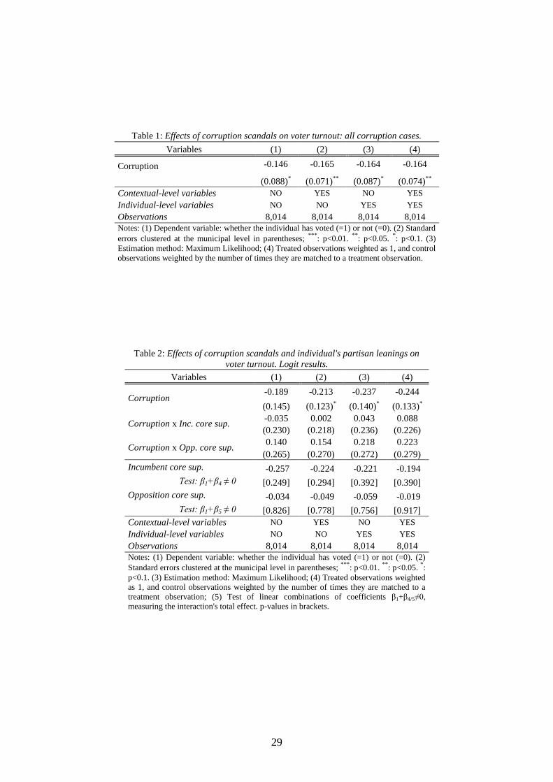
29
Table 1: Effects of corruption scandals on voter turnout: all corruption cases.
Variables (1) (2) (3) (4)
Corruption -0.146 -0.165 -0.164 -0.164
(0.088)* (0.071)
** (0.087)
* (0.074)
**
Contextual-level variables NO YES NO YES
Individual-level variables NO NO YES YES
Observations 8,014 8,014 8,014 8,014
Notes: (1) Dependent variable: whether the individual has voted (=1) or not (=0). (2) Standard
errors clustered at the municipal level in parentheses; ***
: p<0.01. **
: p<0.05. *: p<0.1. (3)
Estimation method: Maximum Likelihood; (4) Treated observations weighted as 1, and control
observations weighted by the number of times they are matched to a treatment observation.
Table 2: Effects of corruption scandals and individual's partisan leanings on
voter turnout. Logit results.
Variables (1) (2) (3) (4)
Corruption -0.189 -0.213 -0.237 -0.244
(0.145) (0.123)* (0.140)
* (0.133)
*
Corruption x Inc. core sup. -0.035 0.002 0.043 0.088
(0.230) (0.218) (0.236) (0.226)
Corruption x Opp. core sup. 0.140 0.154 0.218 0.223
(0.265) (0.270) (0.272) (0.279)
Incumbent core sup. -0.257 -0.224 -0.221 -0.194
Test: β1+β4 ≠ 0 [0.249] [0.294] [0.392] [0.390]
Opposition core sup. -0.034 -0.049 -0.059 -0.019
Test: β1+β5 ≠ 0 [0.826] [0.778] [0.756] [0.917]
Contextual-level variables NO YES NO YES
Individual-level variables NO NO YES YES
Observations 8,014 8,014 8,014 8,014
Notes: (1) Dependent variable: whether the individual has voted (=1) or not (=0). (2)
Standard errors clustered at the municipal level in parentheses; ***
: p<0.01. **
: p<0.05. *:
p<0.1. (3) Estimation method: Maximum Likelihood; (4) Treated observations weighted
as 1, and control observations weighted by the number of times they are matched to a
treatment observation; (5) Test of linear combinations of coefficients β1+β4/5≠0,
measuring the interaction's total effect. p-values in brackets.

30
Table 3: Effects of corruption scandals on voter turnout: timing of corruption. Logit
results.
Panel A (1) (2) (3) (4)
Past corruption cases -0.143 -0.139 -0.151 -0.124
(0.162) (0.135) (0.151) (0.130)
Contextual-level variables NO YES NO YES
Individual-level variables NO NO YES YES
Observations 1,796 1,796 1,796 1,796
Panel B (1) (2) (3) (4)
Recent corruption cases 0.046 -0.000 0.065 0.033
(0.112) (0.112) (0.112) (0.112)
Contextual-level variables NO YES NO YES
Individual-level variables NO NO YES YES
Observations 3,129 3,129 3,129 3,129
Panel C (1) (2) (3) (4)
Repeated corruption cases -0.329 -0.276 -0.384 -0.324
(0.125) ***
(0.116) **
(0.140) ***
(0.118) ***
Contextual-level variables NO YES NO YES
Individual-level variables NO NO YES YES
Observations 3,089 3,089 3,089 3,089
Notes: (1) Dependent variable: whether the individual has voted (=1) or not (=0). (2) Standard errors
clustered at the municipal level in parentheses; ***
: p<0.01. **
: p<0.05. *: p<0.1. (3) Estimation
method: Maximum Likelihood; (4) Treated observations weighted as 1, and control observations
weighted by the number of times they are matched to a treatment observation.
Table 4: Effects of timing of corruption scandals and individual's partisan leanings on voter turnout.
Logit results.
Variables All corruption cases
Past corruption
cases
Recent corruption
cases
Repeated corruption
cases
(1) (2) (3) (4) (5) (6) (7) (8)
Corruption -0.180 -0.244 -0.166 -0.268 0.004 -0.036 -0.309 -0.368
(0.078)**
(0.133)* (0.137) (0.174) (0.119) (0.155) (0.127)
** (0.190)
*
Corruption x Inc.
core sup.
--.-- 0.088 --.-- 0.007 --.-- 0.203 --.-- -0.053
(0.226) (0.382) (0.306) (0.389)
Corruption x Opp.
core sup.
--.-- 0.223 --.-- 0.529 --.-- 0.043 --.-- 0.259
(0.279) (0.305)* (0.287) (0.382)
Incumbent core
sup. --.-- -0.156 --.-- -0.261 --.-- 0.167 --.-- -0.421
Test: β1+β4 ≠ 0 [0.440] [0.439] [0.552] [0.194]
Opposition core
sup. --.-- -0.021 --.-- 0.261 --.-- 0.007 --.-- -0.109
Test: β1+β5 ≠ 0 [0.912] [0.338] [0.976] [0.708]
Contextual-level
variables YES YES YES YES YES YES YES YES
Individual-level
variables YES YES YES YES YES YES YES YES
Observations 8,014 8,014 1,796 1,796 3,129 3,129 3,089 3,089
Notes: (1) Dependent variable: whether the individual has voted (=1) or not (=0). (2) Standard errors clustered at the
municipal level in parentheses; ***: p<0.01. **: p<0.05. *: p<0.1. (3) Estimation method: Maximum Likelihood; (4)
Treated observations weighted as 1, and control observations weighted by the number of times they are matched to a
treatment observation; (5) Test of linear combinations of coefficients β1+β4/5≠0, measuring the interaction's total
effect. p-values in brackets.

31
Table 5: Effects of corruption scandals on voter turnout. Percentage changes in the probability of voting.
Variables
All corruption
cases
Past corruption
cases
Recent corruption
cases
Repeated corruption
cases
(1) (2) (3) (4)
All citizens -0.021 -- -- -0.042
Independent
Voters -0.036 -- -- -0.054
Incumbent core
supporter -- -- -- --
Opposition core
supporter -- -- -- --
Notes: (1) Estimates were generated by running post-estimation simulations of the significant coefficients from Table 4
using the Clarify routine in Stata as described by Tomz et al. (2000), setting each explanatory variable at its mean value;
(2) Dependent variable: whether the individual has voted (=1) or not (=0); (3) Treated observations weighted as 1, and
control observations weighted by the number of times they are matched to a treatment observation; (4) All estimations
include contextual and individual level variables.
Table 6: Effects of corruption scandals on individual's corruption perceptions. Ordered Logit results.
All corruption cases
Past corruption
cases
Recent corruption
cases
Repeated corruption
cases
Variables (1) (2) (3) (4) (5) (6) (7) (8)
Corruption 0.327 0.358 0.194 0.261 0.356 0.417 0.391 0.360
(0.108)***
(0.117)***
(0.163) (0.197) (0.131)***
(0.161)***
(0.1710)**
(0.193)*
Corruption x Inc. core
sup.
--.-- -0.325 --.-- -0.262 --.-- -0.397 --.-- -0.183
(0.146)**
(0.277) (0.216)* (0.227)
Corruption x Opp.
core sup.
--.-- 0.146 --.-- -0.045 --.-- 0.105 --.-- 0.237
(0.130) (0.231) (0.176) (0.182)
Incumbent core sup. --.-- 0.032 --.-- -0.001 --.-- 0.020 --.-- 0.177
Test: β1+β4 ≠ 0 [0.796] [0.997] [0.914] [0.384]
Opposition core sup. --.-- 0.505 --.-- 0.216 --.-- 0.521 --.-- 0.597
Test: β1+β5 ≠ 0 [0.002] [0.339] [0.004] [0.014]
Contextual-level
variables YES YES YES YES YES YES YES YES
Individual -level
variables YES YES YES YES YES YES YES YES
Observations 6,259 6,259 1,387 1,387 2,394 2,394 2,478 2,478
Notes: (1) Dependent variable: Perceptions of local political corruption: 5=Very High Corruption. 4=High. 3=Medium.
2=Low. 1=None. (2) Standard errors clustered at the municipal level in parentheses; ***: p<0.01. **: p<0.05. *: p<0.1. (3)
Estimation method: Maximum Likelihood; (4) Treated observations weighted as 1, and control observations weighted by the
number of times they are matched to a treatment observation; (5) Test of linear combinations of coefficients β1+β4/5≠0,
measuring the interaction's total effect. p-values in brackets.

32
Table 7: Effects of corruption scandals on individual's corruption perceptions.
Simulations.
Variables Perceptions of local political corruption category
None Low Medium High Very High
All Corruption Cases
Independent Voters -0,053 -0,035 0,007 0,049 0,032
Incumbent core supporter -- -- -- -- --
Opposition core supporter -0,056 -0,031 0,009 0,049 0,030
Past corruption cases
Independent Voters -- -- -- -- --
Incumbent core supporter -- -- -- -- --
Opposition core supporter -- -- -- -- --
Recent corruption cases
Independent Voters -0,070 -0,044 0,008 0,066 0,040
Incumbent core supporter -- -- -- -- --
Opposition core supporter -0,075 -0,038 0,010 0,066 0,037
Repeated corruption cases
Independent Voters -0,035 -0,047 0,003 0,048 0,031
Incumbent core supporter -- -- -- -- --
Opposition core supporter -0,039 -0,042 0,006 0,049 0,027
Notes: (1) Estimates were generated by running post-estimation simulations of the
significant coefficients from Table 6 using the Clarify routine in Stata as described by
Tomz et al. (2000), setting each explanatory variable at its mean value; (2) Dependent
variable: Perceptions of local political corruption: 5=Very High Corruption. 4=High.
3=Medium. 2=Low. 1=None; (3) Treated observations weighted as 1, and control
observations weighted by the number of times they are matched to a treatment
observation; (4) All estimations include contextual and individual level variables.

33
Appendix.
Table A.1: Definition of the variables and Summary Statistics
Variable Definition Mean St.Dev. Min Max
Individual-level variables
Turnout Dummy variable coded 1 if the individual voted in the
2007 local elections 0,775 0,418 0 1
Income Self-reported socio-economic classification (1-5): 1: Low;
2: Medium-low; 3: Medium; 4: Medium-High; 5: High 3,357 1,308 1 5
Schooling Highest level of education completed (1-5): 1: any studies;
2: primary; 3: secondary; 4: graduate 46,323 16,697 1 5
Age Age in years 0,499 0,500 18 99
Female Dummy variable coded 1 for females 0 1
Divorced Dummy variable coded 1 for people who are divorced or
separated 0,046 0,209 0 1
Unemployed Dummy variable coded 1 for people who are unemployed 0,142 0,349 0 1
Student Dummy variable coded 1 for students (do not work) 0,058 0,233 0 1
Retired Dummy variable coded 1 for people who are retired 0,208 0,406 0 1
Immigrant Dummy variable coded 1 for people who are not born in
Spain 0,035 0,183 0 1
Corruption
Perceptions
Self-reported perceptions of local political corruption (1-
5): 1: None; 2: Low; 3: Medium; 4: High; 5: Very High
Corruption
2,719 1,313 1 5
Ideology Self-reported ideology (1-3): 1: Left; 2: Centre; 3: Right 1,831 0,711 1 3
Independent Dummy variable coded 1 for people who do not always
vote for the same party 0,512 0,500 0 1
Incumbent core
Supporter
Dummy variable coded 1 for people who always vote for
the same party, and their ideology is the same as the
incumbent's
0,215 0,411 0 1
Opposition
core Supporter
Dummy variable coded 1 for people who always vote for
the same party, and their ideology is the same as the
opposition' party
0,272 0,445 0 1
Contextual-level variables
Corruption Dummy variable coded 1 for municipalities with at least
one corruption scandal in the period 1999-2007 0,482 0,500 0 1
Past
corruption
cases
Dummy variable coded 1 for municipalities with at least
one corruption scandal in the period 1999-2003, but were
not corruption has broke out afterwards
0,110 0,313 0 1
Recent
corruption
cases
Dummy variable coded 1 for municipalities with at least
one corruption scandal in the period 2003-2007, but were
not corruption has broke out before
0,188 0,390 0 1
Repeated
corruption
cases
Dummy variable coded 1 for municipalities with at
corruption scandal in both periods: 1999-2003 and 2007-
2009.
0,185 0,388 0 1
Voter turnout Average voter turnout at the 1987, 1991 and 1995 local
elections 0,687 0,084 0,508 0,922
Income p.c.
Average socio-economic condition. Arithmetic average of
the socio-economic condition according to their
employment status
0,951 0,118 0,610 1,200
Divorced Percentage of divorced and separated among all
population 0,029 0,012 0,002 0,074
Graduate
Percentage of population with third level studies (diploma,
degree and doctorate) among population 16 years and
older
0,128 0,069 0,016 0,434
Unemployment Percentage of unemployed among individuals aged 20-59 0,157 0,079 0,048 0,675
Ethnic diversity
1- Σk(Popk/Population)2 where Pop_contk is population
whose nationality is from continent k, and k refers to
Europe, Africa, America and others
0,058 0,058 0 0,279
Right voters Average historical vote share that the right wing parties
obtained in 1979, 1982, 1986 and 1989 local elections 0,226 0,093 0,037 0,483
log(Population) Log of the registered population 10,545 1,778 6,973 14,957 Notes: (1) Source of the individual-level variables: own-designed survey (see Box A.1). (2) the contextual-level variables: (i)
2001 Census of Population (National Institute of www.ine.es), for Income p.c., % Divorced, % Graduate, % Unemployed,
population by continent used to construct the Ethnic diversity index, and Population. (ii) Database on corruption scandals,
construct (see section 3 for more
details). (iii) Voting data from the Ministry of the Interior, used for the construction of the % Right voters and % Vote turnout variables.

34
Table A.2: Differences in means between Treated and Control groups.
Mean t-test
Treated Control [p-value]
Unmatched sample
% Vote turnout 0.541 0.654 4.25 [0.000]
Income p.c. 0.947 0.939 1.09 [0.282]
% Divorced 0.026 0.018 14.09 [0.000]
% Graduate 0.106 0.077 12.57 [0.000]
% Unemployment 0.147 0.143 0.88 [0.381]
Ethnic diversity 0.060 0.035 10.83 [0.002]
% Right voters 0.507 0.505 0.36 [0.724]
log(Population) 9.610 8.182 27.31 [0.003]
Matched sample
% Vote turnout 0.708 0.692 -1.28 [0.202]
Income p.c. 0.947 0.934 -0.79 [0.428]
% Divorced 0.026 0.026 0.03 [0.976]
% Graduate 0.114 0.104 -1.09 [0.278]
% Unemployment 0.151 0.166 1.23 [0.220]
Ethnic diversity 0.053 0.054 0.08 [0.932]
% Right voters 0.219 0.218 -0.12 [0.908]
log(Population) 9.788 9.678 -0.51 [0.610]
Observations 122 97
Note: (1) Treated group = municipalities where at least one corruption scandal
broke out during the period 1999-2007; Control group=municipalities where
no corruption scandal broke out during the same period.
Table A.3.: Differences in means (survey observations).
Mean t-test
Treated Control [p-value]
Turnout 0.833 0.846 -1.01 [0.220]
Income 2.702 2.721 0.02 [0.479]
Schooling 3.184 3.159 0.03 [0.700]
Age 47.968 47.243 0.72 [0.260]
Female 0.522 0.504 0.02 [0.225]
Divorced 0.044 0.039 0.00 [0.424]
Unemployed 0.130 0.140 -0.01 [0.327]
Students 0.045 0.052 -0.01 [0.222]
Retired 0.241 0.226 0.01 [0.283]
Immigrants 0.039 0.031 0.01 [0.168]
Ideology 1.841 1.817 0.02 [0.324]
Independent 0.510 0.520 -0.01 [0.463]
Incumbent core Supporter 0.224 0.203 1.28 [0.200]
Opposition core Supporter 0.265 0.275 -0.01 [0.507]
Interviewees per municipality 34.779 38.016 -1.18 [0.241]
Number of municipalities 122 97
Note: (1) Treated group = municipalities where at least one corruption scandal
broke out during the period 1999-2007; Control group=municipalities where
no corruption scandal broke out during the same period.