Political Business Cycles through Lobbying∗

Marco BonomoEPGE/FGV and CIREQ

Cristina TerraTHEMA/Université de Cergy-Pontoise and EPGE/FGV

April 9, 2008

Abstract

In this paper we build a framework where the interplay between thelobby power of special interest groups and the voting power of the majorityof the population leads to political business cycles. We apply our set upto explain electoral cycles in government expenditure composition as wellas to cycles in aggregate expenditures and in real exchange rates.

1 Introduction

Over the last decade, there has been a great progress on the understanding

of the mechanisms by which lobbying affects economic outcomes (Grossman

and Helpman 1994, 1996, 2001). In this literature, special interest politics and

elections are linked through campaign contributions. Those are provided by

lobbies in exchange for a tilted economic policy in favor of the interests they

represent.

Another older strand of the political economy literature, the political busi-

ness cycle literature, relates electoral cycles on macroeconomic variable to either

∗We thank Octavio Amorim Neto, Ricardo Cavalcanti, Marcela Eslava, Giovanni Maggi,Jorge Streb, Thierry Verdier and seminar participants at Political Economic Group Seminarat LACEA, IBMEC, CEDEPLAR, EPGE/FGV, PUC-Rio, UnB, EBE-SBE, EEA Meeting,Univeridade Nova de Lisboa, PSE, Paris I and Thema/Cergy-Pontoise for comments and sug-gestions. We also acknowledge financial support from PRONEX. The second author gratefullyacknowledges financial support from CNPq. We thank the hospitality from Bendheim Centerfor Finance, Princeton University, where this research started.

1

partisan (classical references are Hibbs 1977, and Alesina 1987) or opportunis-

tic motives (e.g. Nordhaus 1975, Lindbeck 1976, Cukierman and Meltzer 1986,

Rogoff and Silbert 1988, Persson and Tabellini 1990, and Rogoff 1990), both

unrelated to lobby activity of groups.

While the lobby activity of special interest groups is often associated with

microeconomic policy, and its macroeconomic impact is thought to be negligible,

the political business cycle models explain cycles on aggregate macroeconomic

variables. In this paper we propose a framework in which the influence of

lobbies impact macroeconomic variables that have a distributive effect in society,

generating electoral cycles in those variables.

In the simple framework we propose, opposite interests divide the society

in two groups: one with lobby power1, and the other with the majority of

votes. Government policy may affect the distribution of resources in the society

between those two groups. The lobby group offers the policymaker personal

benefits for a tilted policy in its favor, which is interpreted as corruption, as

further discussed below.

This approach can explain cyclical variation of several macroeconomic vari-

ables around election (e.g. budget variables, inflation, nominal and real ex-

change rate). It is further motivated by the empirical evidence provided by Shi

and Svensson (2006). They find that corruption and rent seeking indicators are

positively related to the size of the electoral fiscal cycle. They also find that

the fiscal balance election year deterioration is only statistically significant for

the group of developing countries. However, when controlling for corruption

and rent seeking indicators, the electoral fiscal cycles are no longer related to

development. The evidence that corruption and rent seeking activities are the

relevant variables to explain electoral cycles is consistent with our model, but

1By lobby power we denote the capacity to influence policy decisions for reasons unrelatedto the number of votes of the group.

2

not with the traditional political business cycle ones.

In our proposed framework, electoral cycles are generated by the interplay

between political influence of a special interest group and the voting power of

the majority of the population. The mechanism behind the cycle is engendered

by the incumbent trying to signal that she has not been captured by the special

interest group, biasing her policy in favor of the majority of the population

before election.

We consider deals that are informal agreements, where the policymaker bi-

ases policy to benefit the lobby group and, in return, is compensated later on.2

For example, former policymakers are often chosen to integrate the supervisory

board of large corporations. Such deals are not self enforcing, hence they de-

pend on a repeated relationship between the policymaker and the lobbyist, in an

environment where some agents interact in several instances over time, possibly

while performing different roles.3

It is, then, reasonable to assume that it may fail to be implemented. That

is, with some probability the deal is implemented and the policymaker receives

the agreed upon amount, but there is some probability the deal falls apart,

resulting on an adverse outcome for the policymaker.4 We think of the success

probability of a deal as depending on factors such as how well the lobby and the

policymaker know each other, how much they trust each other, and what other

relations and connections they have between them.

2 In the special interest literature, such as Grossman and Helpman (1994 and 1996), thepolicymaker first receives the campaign contributions from the lobbies and then implementsthe agreeded upon policy. Here, the policymakers receive illegal or unethical personal benefits,which should be hidden from the public. As the policymaker is subject to more intense mediascrutiny while in office, her compensation is more likely to be given later on.

3This dependence of repeated interactions to enforce a deal is a wider phenomenon, perme-ating the economic relations in economies where the formal institutions are not well developed(see Dixit 2004).

4This adverse outcome may be explained by the deal may becoming public, resulting in anelection defeat, as in the variant of the model developed in Appendix A. Another possibilityis that the unsuccessful deal is not revealed to the public but the policymaker dislikes beingbetrayed.

3

The voters do not observe the success probability of a deal between the

lobby and the incumbent because they are not aware of all connections between

them. Neither they observe whether a deal between them was set. They can

not perfectly infer that information either, for we assume economic policy is

observed with noise.5

The median voter would like to pick the politician with less connections with

the lobby, since it will be more likely that she will not set a deal with the lobby

after election. To increase her reelection probability, in the period before election

the policymaker close to the lobby has an incentive to disguise her proximity.

She does so by choosing a policy less favorable to the special interests group than

the one she would choose if there were no reelection concerns. Analogously, the

policymaker far from the lobby, on her turn, will tilt her policy in favor of the

majority group to signal her distance. This behavior generates policy variables

cycles around election.

The model generates an additional cycle, which is a “contracting” cycle

around elections. Since reelection concerns induce the policymaker to favor

less the special interest group, the mutual net gains from a deal between the

incumbent and the lobby are reduced before elections. Therefore, it is less likely

that the policymaker will make a deal with the lobby before elections than after

elections.6

This setup has several applications. With regard to the overall government

budget, the distribution in the population of the benefit of government expenses

net of the costs of taxation is unequal. For several countries, it is plausible to

assume that the fiscal situation is such that the large majority of the population

would benefit from an increase in government expenses. A smaller group, for

5This assumption is consistent with Downs (1957) analysis, according to which an indi-vidual voter does not have the incentive to spend resources to get informed, since she cannotaffect the election results.

6This is in contrast with specific interests lobbying activity where politicians are rewardedwith campaign contributions reward in exchange of microeconomic policy biases.

4

which the cost would exceed the benefit, would have an incentive to organize

themselves to lobby for lower taxation. According to our approach, the result

would be a budget cycle around election, which, depending on institutional

details, could yield either a simultaneous increase in expenses and taxation or

an increase of the fiscal deficit before elections. This is consistent with the above

mentioned evidence in Shi and Svensson (2006).

When the public expenditures are specific to groups in society our model is

able to generate electoral cycles in the composition of government expenditures.

This is in line with the recent empirical evidence of electoral cycles on the

composition of the fiscal budget (on Canada, see Kneebone and McKenzie 2001;

on Mexico, see Gonzalez 2004; on Colombia, see Drazen and Eslava 2005a).

Our model can also be applied to explain real exchange rate cycles around

elections. Movements in the exchange rate have a distributive impact, favoring

citizens whose income is positively related to prices of tradable goods in detri-

ment to citizens with income linked to nontradable prices. In countries where

the nontradable group entails the majority of the population while the tradable

group has lobby power, one could expect to see more appreciated exchange rates

before than after elections. There is strong empirical evidence of this type of

cycle in Latin American countries (see Frieden, Ghezzi and Stein, 2001, and

Ghezzi, Stein and Streb, 2004, for cross-country evidence, Bonomo and Terra,

2001, Grier and Hernández-Trillo, 2004, and Pascó-Fonte and Ghezzi, 2001, for

Brazil, Mexico and Peru, respectively).

Our model has some distinctive features. The association with lobbies is

politically costly to the incumbent. In this respect, it differs from the special

interests politics literature. Here, setting a deal with the lobby jeopardizes her

reelection chances instead of improving it, as in that literature. This difference

stems from the type of policy variable the lobby aims at in the two contexts.

The special interest politics literature explains the impacts of lobbying on mi-

5

croeconomic variables. The level of such variables has less widespread effect

over the populations. Hence it should not impact significantly election results.

There are three dimensions in which our model departs from previous po-

litical business cycle models. First, the key tension is on the distribution of

resources between two groups in society: one with the lobby power, and the

other with the voting power. This allows us to generate cycles not only in the

level of macroeconomic variables that have distributive impact, but also directly

in distributive variables.

Second, the incumbent’s motivation for being reelected is the possibility

of receiving personal benefits for favoring the lobby after elections, which will

depend on her policy choice. Hence, we have built in an endogenous rent from

being in office, instead of resorting to the usual exogenous ‘ego rents’.

Third, it mixes adverse selection and moral hazard features. The first gen-

eration of PBC rational models, initiated by Rogoff and Silbert (1988) and

Rogoff (1990), is characterized by hidden information about the policymaker’s

competence, who chooses an action to signal her type. In equilibrium her type

will be revealed. An unappealing feature of these models is that only the most

competent incumbent distorts policy.

A more recent generation of PBC models proposes a moral hazard frame-

work to handle this problem (e.g. Lohmann 1998, Persson and Tabellini 2000,

and Shi and Svensson 2002). They propose a simple twist in the adverse models:

the incumbent chooses her action before knowing her own type. This assump-

tion impels both types of incumbents to choose the same policy. Although the

incumbent’s action is not observed by the electorate, the observed economic out-

come ends up revealing her type as it is determined by the interaction between

her competence and the chosen policy. Those models generate the desired result

- in equilibrium both types distort policy-, at the expense of an unappealing one

- both types choose the same policy.

6

In our framework, different types of incumbents choose different policies,

as in the adverse selection models, and distort policies before elections, as in

the moral hazard models. The main departure from adverse selection models

driving our results is that policy is observed with noise. This assumption yields

the incentive for both types to distort policy, as the incumbent’s type can never

be perfectly inferred by the voters.

This feature has some important implications. One advantage of a noisy

signal is that a large range of results is consistent with the equilibrium strate-

gies, each one leading to a different belief on the incumbent’s type. Then, the

equilibrium does not depend on the arbitrary specification of out of equilibrium

beliefs, which is common in signaling models. Moreover, we do not need to

assume an exogenous popularity or ‘looks’ shock to make the election result

uncertain, as in the adverse selection models.

Other models relate to this paper in generating cycles in distribution of

resources. In Bonomo and Terra (2005), an exchange rate cycle distributes

income between tradable and nontradable sectors. Voters are unsure about the

weight given to their group in the policymaker’s preference, and observe policy

with a noise. Exchange rate cycles around elections are thereby generated. In

Drazen and Eslava (2005b), voters suffer from the same information asymmetry

with respect to the incumbent’s preferences but are also uncertain about how

sensitive is their group’s voting behavior to government expenditures. The

result is a cycle in expenditure composition. Another alternative model of cycle

in the expenditure composition is provided by Drazen and Eslava (2005a), where

policymakers preferences are formulated in terms of types of expenditures.

We start by developing the basics of a simple but general framework in

the next section. In section three we solve the optimal policy problem under

lobby influence in a one period setting. The dynamic problem is studied in

section four. In section five we provide three applications to the model. In

7

the first one, presented in more detail, government chooses the composition of

expenditure between the two groups. In the second application, we generate

political budget cycles by assuming that increase in government expenditures

benefit the majority of the population, while the lobby group is hurt when

taxes are increased. Finally, we have an exchange rate model, engendering real

exchange rate cycles around election, when we associate the tradable sector to

the lobby while the nontradable sector is assumed to have the voting power. In

this context, the policy variable is the real exchange rate level. The last section

concludes.

2 Model Set up

Society is divided into two groups. One group, which we call people, is the

majority (proportion n of the population, n > 0.5), and defines the elections

outcome. The other group is organized and effective in lobbying for policies

that favor their interests.

Government chooses an economic policy, which, for convenience, we model

as a strictly positive variable g. This policy affects utility of the two groups

in opposite directions. Let vi (g) be the indirect utility function of a citizen of

group i, i = p (people), l (lobby), when the policymaker implements policy level

g. Without loss of generality, we assume that the people benefit from higher

values of g, whereas, for the lobby, the lower the g the better. That is, v0p (.) > 0

and v0l (.) < 0. We also assume vi (.) to be concave.

We assume that the welfare function of a benevolent policymaker is utilitar-

ian:

U (g) = nvp (g) + (1− n) vl (g) , (1)

hence she would optimally choose:

g∗ ≡ U 0−1 (0) . (2)

8

We add the possibility that policymaker receives some personal benefit from

the lobby in exchange of a policy choice favoring this group. We extend the

lobby and policymaker preferences to contemplate this more complex interaction

between them. Now, the policymaker’s utility depends not only on the direct

impact of his policy choice g on the groups’ utilities but also on the personal

benefits and losses that may result from his interaction with the lobby group.

The personal benefits she may receive from the lobby, c (g), depends on the

distortion of policy in favor of this group. More specifically, we assume that she

is able to take hold of a portion B from the net gain she creates to the lobby

group by distorting policy in its favor, that is:

c (g) = B (1− n) [vl (g)− vl (g∗)] . (3)

This can be interpreted as being a result of a Nash bargain, where B depends

on the bargaining power of the policymaker vis-a-vis the lobby group.7

As discussed in the introduction, we think of those deals as informal agree-

ments where the policy is chosen first and the personal benefits will be received

in the future. Therefore, it is possible that the policymaker does not receive

the contribution, since such deals are not self enforcing. The probability that

the policymaker will receive the agreed upon benefit later on depends on factors

such as extent of their repeated interaction, on the ability of the policymaker

to punish the lobbyist in other dimensions. We take these connections between

the lobbyist and the policymaker as exogenous, and determining the probability

π that the deal is successful. This probability will be the source of the informa-

tion asymmetry between the policymaker and the median voter in the dynamic

setting.8

7One may argue that, once the policy is chosen, the lobbyist has all the bargaining power.However, we think of this bargaining as being determined by the repeated interaction betweenthe policymaker and the lobbyist along their lives.

8The variable that determines the type of the policymaker could be bidimensional, depend-ing not only on the probability of a successful deal, but also on the bargaining power of thepolicymaker. For simplicity we ignore this extra dimensionality.

9

When the policymaker does not receive the agreed upon benefit she incurs

in a reduction of X in her utility, instead of an increase of c (g). We interpret

this as an emotional cost from being deceived. An alternative interpretation

is that, when the deal falls apart, it is revealed to the public. This revelation

changes the policymaker’s reelection probability, which, in this case, leads to a

loss incurred in case of a broken deal. We explore this venue in Appendix A.

The policymaker chooses ex-ante whether to set a deal with the lobby group

to distort policy in its favor or not so as to maximizing her utility function,

which in this particular situation can be represented by:

W (g, I, π) = nvp (g) + (1− n) {vl (g)− IπB [vl (g)− vl (g∗)]}+

+I {θπB (1− n) [vl (g)− vl (g∗)]− (1− π)X} ,

where I is a indicator function that equals 1 when the policymaker set a deal

with the lobby group and zero otherwise. The equation can be written as:

W (g, I, π) = U (g) + I {πb [vl (g)− vl (g∗)]− (1− π)X} , (4)

where b ≡ (1− n) (θ − 1)B.

3 One period problem

Let G be the optimal policy level chosen by the government if there were only

one period, with no election concerns. We derive the optimal policy choice under

a deal (I = 1) and when no deal is set (I = 0). The optimal contracting decision

is the one that yields the policymaker the highest utility.

In this one period setting, the optimal policy choice when there is no deal

with the lobby is that of the benevolent policymaker, that is, G = g∗.

The optimal policy level when there is a deal between the policymaker and

the lobby is defined by:

g# = argmaxW (g, 1, π) ,

10

which is implicitly defined by the first order condition:

Wg

¡g#, 1, π

¢= U 0

¡g#¢+ πbv0l

¡g#¢= 0. (5)

Proposition 1 The policy choice under a deal with the lobby favors the lobby

group to the detriment of the people when compared to the utilitarian policy,

that is, g# < g∗. Furthermore, the policymaker will favor more the lobby group

under a deal the higher its probability of success, that is, dg#

dπ < 0.

Proof. Using equation (2), we have that Wg (g∗, 1, π) = πbv0l (g

∗) < 0. Since

W (.) is concave in g, g# < g∗. Using the implicit function theorem in the first

order condition (5), we have that dg#

dπ = − bv0l(g#)

U 00(g#)+πbv00l (g#)

< 0.

The incumbent will choose to set a deal with the lobby, distorting the policy,

if her welfare under the deal is higher than the one when there is no deal. That

is, she will accept to set a deal with the lobby and distort the policy whenever:

W¡g#, 1, π

¢≥W (g∗, 0, π) .

Hence, the equation:

W¡g#, 1, π

¢=W (g∗, 0, π) (6)

defines the probability π for which the incumbent is indifferent between setting

or not a deal with the lobby.

It is easy to see that the left hand side of equation (6) is increasing in π,

while the right hand side is independent of π. Thus, π is a cutoff level such that

the government sets the deal with the lobby whenever π ≥ π.

We can summarize the results above in the following proposition.

Proposition 2 For given values of n, X and b, there is a cutoff probability π,

0 < π < 1, defined implicitly in equation (6), such that the incumbent will set a

deal with the lobby if, and only if, π ≥ π.

11

If π < π, then g = g∗.

If π ≤ π, then g = g# < g∗, where g# is defined implicitly in equation (5).

4 The dynamic problem

In this section we solve the dynamic problem, where there is an election at every

other period. The main features of our story can be told in a simpler and clearer

two-period setup, with an election between them. In Appendix B we sketch a

more general multiperiod framework to show the results obtained in the two

period set up described in this section would still hold.

The success probability of a deal π is the source of information asymmetry

between the policymaker and the median voter. We assume that there are two

types of policymakers, f and c, with πf < πc, reflecting the connection strength

between the policymaker and the lobbyist.9

Those connections are likely to be persistent, since they are forged in a

long-run relationship between the incumbent and the lobbyist. However, the

deal is established by individuals in government and lobby key positions. The

assignment for those positions may change, even over the same mandate. In

order to capture those features in the simplest way we assume the types to be

randomly assigned to the politician in the period before election from a Bernoulli

distribution, with Pr (π = πf ) = p and Pr (π = πc) = 1− p.10

4.1 After election problem

Since the after election period is the last one, there is no signaling component

in the government’s policy decision then.11 In this case, the proposition 2 for

9 In our notation, f stands for "farther from the lobby" and c for "closer to the lobby".10A popular alternative used in the literature is to assume that the policymaker’s specific

characteristic is determined by a MA (2) process, as, for example, in Rogoff (1990). Thiswould generate equilibria with four different policy choices for the government at each period,unecessarily complicating the analysis.11Note that it is also true that there is no signaling component in the government’s policy

decision after election in the multiperiod setting, since there is a new draw for the policy-

12

the static problem still applies.

Thus, the after election optimal policy is given by:³Gj+1, I

j+1

´=

½ ¡g#, 1

¢if πj ≥ π

(g∗, 0) otherwise(7)

where Gj+1 and I

j+1 are, respectively, the after election optimal expenditure and

decision of having a deal with the lobby or not for policymaker of type j, π is

defined implicitly in equation (6), and g# in equation (5). Since πc > πf , from

Proposition 1 we have that Gc+1 ≤ Gf

+1 ≤ g∗. Thus, we established that after

elections the policy maker closer to the lobby will distort more the policy than

the farther type.

4.2 Pre-election problem

4.2.1 The voter’s problem

We assume that the government policy is observed with a noise. Specifically,

we assume that the people observe the variable bg, which is given by:bg = geυ,

where υ is a Gaussian shock with mean zero and variance σ2. This can be

rationalized as resulting from voters’ rational inattention.12

We also assume that the people do not observe the policymaker’s type π.

Hence, voters will try to infer π, given the observed policy. There will be a

signaling game between the incumbent and the voters.

The median voter, not belonging to the lobby group, would like to vote for

the policymaker who will choose a policy more favorable to the people after

election. It is clear from Proposition 1 that this will be the policymaker farthest

from the lobby, πf . Since there is no information about the opposition, it is

maker’s type in between elections.12Citizens have limited information capacity and they have several other decision problems

to solve that depend on information. Thus, it is reasonable to assume that, as a result, theywill be imperfectly informed about most of the relevant variables. See Sims (2003) for someapplications of rational inattention to economic problems.

13

assumed that the probability of it being far from the lobbyist is equal to the

unconditional probability.

The median voter chooses her candidate by comparing the (updated) prob-

ability of the incumbent being of type πf to that of the opponent. As the

opponent is not in power, it is assumed that the probability that she is of type

πf is equal to the unconditional probability p. Thus, if the updated probability

about the incumbent’s type is larger than p, people will vote for the incumbent,

and she will be reelected. Otherwise the opponent will win the election. If

the updated probability is equal to the unconditional probability, we assume

that the incumbent is reelected with probability 12 . Let ρ be the median voter’s

conjecture that the incumbent is far from the lobby, and vo his vote. Then:

vo =

⎧⎨⎩ inc, if ρ > popp, if ρ < p

inc with probability 12 if ρ = p

.

How do voters form their belief ρ? Given the lognormality assumption for the

noise, any level of observed policy could result from any given policy. Therefore,

every positive level for the observed policy is in the equilibrium path. The

median voter’s belief ρ is generated by the updating of his prior belief p over

the incumbent’s type using Bayes’ rule:

ρ = Pr (πt = πf |bgt = bg ) = (8)

=p× f(bgt = bg |πt = πf )

p× f(bgt = bg |πt = πf ) + (1− p)× f(bgt = bg |πt = πc ),

where bg is the observed policy level, and f(. |. ) is the conditional density functionof bg given the policymaker’s type. The voter will vote for the incumbent, thatis ρ > p, if and only if:

f(bgt = bg |πt = πf ) > f(bgt = bg |πt = πc ). (9)

This rule is intuitive. The voter revises upwards his prior that the govern-

ment is of the distant type if, and only if, the observed policy level is more likely

14

under the distant type’s policy than under the policy chosen by the type closer

to the lobby.

4.2.2 Reelection probability

Now we can calculate the incumbent’s reelection probability as a function of the

chosen policy level. To do so, it is necessary to specify the incumbent’s actions

prescribed by the equilibrium strategy in the period before election©Gf , Gc

ª,

which will be used by the voter to update his beliefs.

A chosen expenditure level g and a noise υ will determine the observed

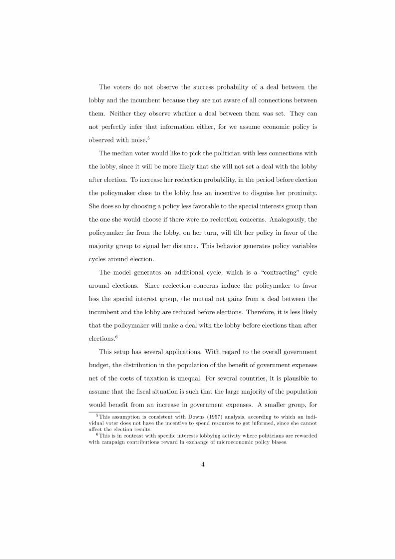
policy level, bg = geυ. Therefore, the conditional density function of bg given thepolicymaker’s type, f(. |. ), is equal to the density function of the noise υ that

would yield bg when the policy level is the one chosen by this type in equilibrium.That is,

f(bgt = bg |πt = πi ) = φ

µln bg − lnGi

σ

¶(10)

where φ is the density of the standard normal distribution. Figure 1 illustrates

the density function of the observed policy, for a given policy chosen.

Figure 1: Observed policy density function

15

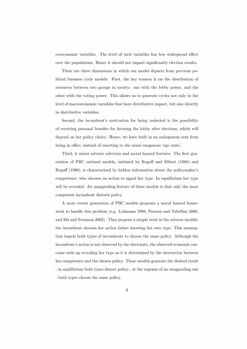
Figure 2: Policy Cutoff Level

Then, we can write the conditions for reelection in equation (9) as:

φ

µln bg − lnGf

σ

¶> φ

µln bg − lnGc

σ

¶. (11)

In the case of a separating equilibrium, with Gf > Gc, the policy has a cutoff

level g, such that, whenever the observed policy level is larger than g (bg > g),

the median voter reelects the incumbent. This policy cutoff level is implicitly

defined by:

φ

µln g − lnGf

σ

¶= φ

µln g − lnGc

σ

¶which, due to the symmetry of the normal distribution, is:

g = exp

∙lnGf + lnGc

2

¸.

Figure 2 depicts the density functions of the observed policy when the policy

level is the one chosen by each type of incumbent in equilibrium, πf and πc. The

figure also shows the cutoff level of the observed policy g. Note that condition

(11) is satisfied for bg > g.

16

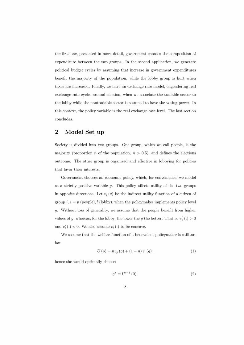
Figure 3: Probability of reelection

For a chosen policy g, the reelection probability, q (.), is the probability that

the observed policy, bg, exceeds the cutoff point, g,13 that is:q¡g,Gf , Gc

¢≡ Pr [bg > g] = Pr [geυ > g] =

= Pr [υ > ln g − ln g] ,

which can be written as:

q¡g,Gf , Gc

¢= 1− Φ

µln g − ln g

σ

¶,

where Φ (.) is the normal cumulative distribution function. The reelection prob-

ability is increasing in g, and it is greater than 12 if, and only if, g > g. Figure

3 illustrates the probability of reelection for a chosen policy level g and for the

two types of incumbent equilibrium strategies, Gf and Gc, which determine g.

Suppose, alternatively, that there is a separating equilibrium with Gc > Gf

(we will see in section 4.3 that this equilibrium is not possible). Then, since13More precisely, the probability of reelection is equal to the probability of the observed

expenditure being strictly greater than the cutoff level plus half the probability of the ob-served expenditure coinciding exactly with the cutoff level. However, under our continuousdistribution assumption, the latter probability is zero.

17

voting is prospective, the median voter will still prefer the policymaker further

away from the lobby, although she will choose a lower policy level before election.

As a consequence, the inference problem is reversed, and the probability of

reelection as a function of policy level and equilibrium strategy will become:

q¡g,Gf , Gc

¢= Φ

µln g − ln g

σ

¶,

Now q is decreasing in g, since a lower g increases the probability that the

incumbent is of the distant type.

Finally, in the case of a pooling equilibrium, we have always ρ = p. Thus,

the probability of reelection is 12 and will not be affected by any deviation from

equilibrium strategy.

Then, we can summarize the dependence of the probability of reelection

function on the various types of candidate equilibria as follows:

q¡g,Gf , Gc

¢=

⎧⎪⎪⎨⎪⎪⎩1− Φ

³ln g−ln g

σ

´, if Gf > Gc

Φ³ln g−ln g

σ

´, if Gf < Gc

12 if Gf = Gc

, (12)

where g = exphlnGf+lnGc

2

i.

4.2.3 The Incumbent’s Strategy

Let FW (πi) be the after election utility of the type πi government, when re-

elected:

FW (πi) ≡W¡Gi+1, I

i+1, πi

¢where Gi

+1 is the expenditure and Ii+1 is the decision of setting or not a deal

with the lobby, optimally chosen after elections by the reelected incumbent of

type πi (refer to section 4.1). Note that:

FW (πi) ≥ U (g∗) , (13)

since it is always possible to the policymaker not to make a deal with the lobby

and to choose policy level g∗. Moreover, the policymaker will be strictly better

18

off being reelected if her proximity to the lobby enables her to get rents from

being in power.

When the incumbent is not reelected her utility will be the benevolent one,

since we assume that there is no additional source of personal income or loss of

reputation when the policymaker is not in office. Alternatively, we can motivate

this specification by assuming that the policymaker will become a member of

the majority group with probability p and a member of the lobby group with

probability 1−p. Let FU be the expected after election utility of the incumbent,

when she is not reelected:

FU = pU³Gf+1

´+ (1− p)U

¡Gc+1

¢.

Since the policymaker will have no rents when she is not reelected, the best

outcome for her is to have the new incumbent setting the socially optimal policy

level g∗. When at least one of the opposition possible types chooses to set a deal

with the lobby, an assumption we make,14 her policy choice yields the defeated

policymaker a lower utility compared to that resulting from g∗, thus:

FU < U (g∗) . (14)

Combining equations (13) and (14), we have that:

FU < FW (πi) . (15)

This last inequality implies that the policymaker always strictly prefers to

be reelected. Note that the benefit from being in power is generated by the

potential deal between the policymaker in power and the lobby. Since this

benefit will depend on the policy implemented, it is endogenous. The difference

14As we argue in section 4.3, after elections the incentives are more favorable to a deal. Ifwe assume functional forms and parameter values such that no deals are set after elections,the model will generate only an uninteresting pooling equilibrium with the utilitarian policyg∗ chosen before and after elections.

19

FW (πi) − FU has the same role as the exogenous “ego rents” from being in

power extensively used in the political economy literature.

In equilibrium, the two decisions - the policy level and whether to set a deal

or not with the lobby - will be chosen so as to solve:

maxg,I

©V¡g, πi, I,G

f , Gc¢ª

(16)

s.t. g > 0,

where:

V¡g, πi, I,G

f , Gc¢=W (g, πi, I)+ (17)

+β£q¡g,Gf , Gc

¢FW (πi) +

¡1− q

¡g,Gf , Gc

¢¢FU

¤,

and where β is the incumbent’s discount rate and the function q is given by

equation (12).

Equation (17) can be rewritten as:

V¡g, πi, I,G

f , Gc¢= (18)

W (g, πi, I) + βq¡g,Gf , Gc

¢[FW (πi)− FU ] + βFU,

which makes clear that a higher reelection probability increases the utility of

the incumbent whenever it is advantageous for at least one of the types to set a

deal with the lobby after election.

Whenever reelection increases utility, the incumbent policymaker will choose

a policy which will depart from the static optimal level, which maximizes only

W (g, πi, I). As we will show below, the only type of equilibrium consistent with

this possibility has Gf > Gc. This makes q increasing in g (equation (12)),

and the optimal level of g higher than the static one for both types. As the

after election policy choices coincide with the static optimal choices, there will

be policy cycles around elections, with policy favoring more the people before

20

elections than after elections.15

4.3 Equilibrium

An equilibrium requires a fixed point in the solution of the incumbent problem

(16). That is:

Gc = argmaxg,I

©V¡g, πc, I,G

f , Gc¢ª

(19)

s.t. g > 0,

and:

Gf = argmaxg,I

©V¡g, πf , I,G

f , Gc¢ª

(20)

s.t. g > 0.

A perfect Bayesian equilibrium in pure strategies, when it exists, should

satisfy the following conditions:

1. After election, an incumbent of type j will choose to set a deal with the

lobby whenever her type satisfies: πj > π, where π is defined implicitly

by equation (6). She sets policy level g# (which is implicitly defined by

equation (5)) if she has a deal with the lobby and g∗ (defined by equation

(2)) otherwise;

2. Before election, an incumbent chooses whether to set a deal with the lobby

and the policy level so as to maximize her expected intertemporal utility

function, that is, to solve problem (16), where the probability of reelection

function, q(g,Gc,Gf ), is given by expression (12);

15Formally, we have that∂W (Gj+1,πi,I)

∂g= 0. Hence,

∂V³Gj+1, πi, I,G

f , Gc´

∂g=

∂W (Gj+1, πi, I)

∂g+ β

∂q³Gj+1, G

f , Gc´

∂g[FW (πi)− FU ]

= β∂q³Gj+1, G

f , Gc´

∂g[FW (πi)− FU ] > 0.

21

3. Before election, the policy level chosen by each type of policymaker is a

fixed point, that solves problems (19) and (20), respectively.

We assume that the parameter values are such that the type closer to the

lobby benefits from a deal with the lobby after election. This will produce an

equilibrium with the following features. First, it must be the case that Gf > Gc,

since an equilibrium with Gf < Gc is not possible.16

Second, there will be policy cycles around elections, that is, the policy favors

more the people before elections than after. More precisely, whenever it is

advantageous to at least one of the policymaker types to make a deal with the

lobby after elections, there will be electoral incentives that stimulate a policy

more favorable to the poor before election than after for each policymaker type.

The third feature is that a deal between the policymaker and the lobby is

more likely to happen after election than before. More specifically, whenever

an incumbent of a certain type makes a deal with the lobby before election,

she will also do it after election, but the converse is not true. A deal with

the lobby is profitable for the incumbent only if the policy favors substantially

that group. However, election concerns induce the policymaker to set a policy

more favorable to the people, reducing the gain of an agreement with the lobby.

Therefore an agreement with the lobby is less likely before elections.

There is no guarantee that a pure strategy equilibrium exists. The model

may not have an equilibrium if the type closer to the lobby benefits only mar-

ginally from a deal with the lobby after election. The argument is outlined in

Appendix C. However, a parameter configuration which leads to no equilibrium

is not plausible in the context of the present model. The model relies on the pos-

sibility of deals between the policymaker and the lobby, and on non-observable

16As the type πc has higher rents from being reelected, his chosen policy before election willbe more distorted to increase his reelection probability. As the reelection probability functionwould be decreasing in g in this case, before election the type πc would choose a policy levelactually lower than that of type πf , leading to a contradiction.

22

comparative advantages of certain types to benefit from those deals. Thus, it

is reasonable to assume that those deals benefit substantially, rather than mar-

ginally, the policymaker that have access to them (the closer type, πc) under

the most favorable conditions to them, that is, after elections.

5 Applications

5.1 Government expenditure cycles

5.1.1 Expenditure composition cycles

There is evidence of electoral cycles on the composition of the fiscal budget in

several countries (on US, see Peltzman 1992; on Canada, see Kneebone and

McKenzie 2001; on Mexico, see Gonzalez 2004; on Colombia, see Drazen and

Eslava 2005). We now show how the framework developed above can be applied

to generate such electoral expenditures composition cycles.

In the simple formulation we choose the budget is always balanced, taxes

are fixed and there are two types of public goods, specific to each of the two

groups. The government budget constraint is represented by:

τ = (1− n) gl + ngp,

where τ are taxes per capita that are uniform over the population, gl and gp

are expenditures for the lobby and for the people, respectively (all per capita).

It can be rearranged as:17

gl =τ − ngp1− n

.

The utility function of a citizen of group i, ui, is represented by:

ui (ci, gi) = ci + log gi, for i = p, l, and α > 1,

17Note that, in this case, it is economically reasonable to impose an upper bound for gp(0 < gp ≤ τ

n) to prevent a negative value for gl. However, this new restriction is never binding

in equilibrium.

23

where ci is her private consumption, and gi is the amount of the public expen-

diture available to her group. Given that ci = yi − τ , indirect utility functions

may be written as:

vl (g) = yl − τ + log

µτ − ng

1− n

¶, and (21)

vp (g) = yp − τ + log g, (22)

where we use g ≡ gp for simplicity.

Substituting equations (21) and (22) into the utilitarian welfare function of

a benevolent policymaker, represented by equation (1), we get:

U (g) = y − τ + n log g + (1− n) log

µτ − ng

1− n

¶, (23)

where y = nyp + (1− n) yl is the average per capita income. The benevolent

policymaker would optimally choose:

g∗ = τ = gl, (24)

that is, all citizens would receive the same spending level.

The optimal spending level under a deal in a one-period setting, that is, the

spending level that satisfies equation (5), is given by:

g# =τ

1 + πb. (25)

Note that in this application we have an explicit solution for the spending level.

It is easy to check Proposition 1: g# < g∗ and g# is decreasing in π.

The cutoff probability π defined by equation (6) now becomes implicitly

defined by:

(1− n+ πb) log1− n+ πb

(1− n)− (1 + πb) log (1 + πb) = X (1− π) . (26)

Following the setup above, we are able to show that there will be an electoral

cycle in the expenditures composition, with more spending for the people before

than after election. We provide a numerical example to illustrate the model’s

ability to generate electoral cycles.

24

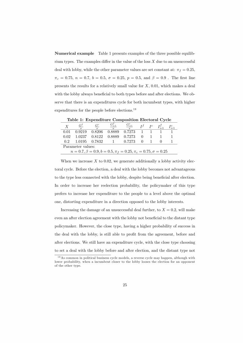
Numerical example Table 1 presents examples of the three possible equilib-

rium types. The examples differ in the value of the loss X due to an unsuccessful

deal with lobby, while the other parameter values are set constant at: πf = 0.25,

πc = 0.75, n = 0.7, b = 0.5, σ = 0.25, p = 0.5, and β = 0.9 . The first line

presents the results for a relatively small value for X, 0.01, which makes a deal

with the lobby always beneficial to both types before and after elections. We ob-

serve that there is an expenditures cycle for both incumbent types, with higher

expenditures for the people before elections.18

Table 1: Expenditure Composition Electoral Cycle

X Gf

τGc

τ

Gf+1

τ

Gc+1

τ If Ic If+1 Ic+10.01 0.9219 0.8206 0.8889 0.7273 1 1 1 10.02 1.0237 0.8122 0.8889 0.7273 0 1 1 10.2 1.0195 0.7832 1 0.7273 0 1 0 1Parameter values:

n = 0.7, β = 0.9, b = 0.5, πf = 0.25, πc = 0.75, σ = 0.25

When we increase X to 0.02, we generate additionally a lobby activity elec-

toral cycle. Before the election, a deal with the lobby becomes not advantageous

to the type less connected with the lobby, despite being beneficial after election.

In order to increase her reelection probability, the policymaker of this type

prefers to increase her expenditure to the people to a level above the optimal

one, distorting expenditure in a direction opposed to the lobby interests.

Increasing the damage of an unsuccessful deal further, to X = 0.2, will make

even an after election agreement with the lobby not beneficial to the distant type

policymaker. However, the close type, having a higher probability of success in

the deal with the lobby, is still able to profit from the agreement, before and

after elections. We still have an expenditure cycle, with the close type choosing

to set a deal with the lobby before and after election, and the distant type not

18As common in political business cycle models, a reverse cycle may happen, although withlower probability, when a incumbent closer to the lobby looses the election for an opponentof the other type.

25

setting the deal at any time.

Finally, an increase of X to the point that prevents any deal with the lobby

(not presented in the table) will result in an not very interesting type of equilib-

rium. Both types choose to spend τ for both types of citizens, before and after

elections.

5.1.2 Aggregate expenditure cycles

Electoral cycles in aggregate expenditures can be generated by a simple change

in the model described above. Suppose that the people are not taxed and receive

the only public good. Indirect utility functions become:

vl (g) = yl − τ , and (27)

vp (g) = yp + log g. (28)

We still assume a balance budget: g = τ .

An utilitarian policymaker without lobby influence and electoral incentives

will choose:

g∗ =n

1− n.

If she has a deal with the lobby, she will choose:

g# =n

1− n+ πb=

g∗

1 + g∗πbn

. (29)

With information asymmetry about the two different policymaker types, πc

and πf , as before, the model generates electoral cycles in aggregate expenditures.

This result is in line with the empirical evidence, as in Brender and Drazen

(2004), Shi and Svensson (2002a,b), and Persson and Tabellini (2002).19

19Note that the balanced budget assumption also generates a counterfactual electoral taxcycle. In a more complex version of the model, we could assume, instead, that taxes are hardto change and that any eventual budget imbalances could be financed by government debt.This setting would generate an intertemporally balanced budget equilibrium with electoralbycle in expenditures and budget deficits.

26

5.2 Exchange rate cycles

There is empirical evidence of exchange rate electoral cycles for Latin American

countries (cross-country evidence for Latin America is provided by Frieden,

Ghezzi and Stein, 2001, and Ghezzi, Stein and Streb, 2004, for Brazil, see

Bonomo and Terra, 2001, Grier and Hernández-Trillo, 2004, for Mexico, and

Pascó-Fonte and Ghezzi, 2001, for Peru). Bonomo and Terra (2005) presents

a model that generates real exchange rate electoral cycles, in a setting with

informational asymmetry over the policymaker’s preferences. Here we derive

the same result in a simpler model based on lobby politics proposed in this

paper.

Consider a endowment economy with two sectors: a tradable a nontradable

sector. The nontradable sector has the majority of the population, while the

tradable sector has the lobby power. All consumers are assumed to have the

same CES utility function:

u (Ni, Ti) =³N

r1+r

i + Tr

1+r

i

´ 1+rr

, (30)

where Ni and Ti are the amount consumed of nontradable and tradable goods,

respectively, and r > 1. Now let e be the tradable good relative price, which is

the real exchange rate. Define g ≡ 1e . As expected, the indirect utility function

is decreasing in the real exchange rate for a citizen in the nontradable sector,

and increasing for the tradable sector:

vN (g) =¡1 + g−r

¢− 1r EN , and (31)

vT (g) = (1 + gr)−1r ET , (32)

where EN and ET are the per capita endowment for the nontradable and trad-

able sectors, respectively.

A benevolent (utilitarian) policymaker would choose to set the exchange rate

27

at a level:20

g∗ =

µnEN

(1− n)ET

¶ 1r−1

. (33)

The policymaker may choose to set a more depreciated exchange rate, g < g∗

(which means e > e∗ ≡ 1g∗ ) in order to favor the tradable sector and get a share

of its gain. Proceeding as before, we find that whenever there is an agreement

with the tradable sector the chosen exchange rate is given by:

g# =

µnEN

(1− n)ET + πbET

¶ 1r−1

(34)

= g∗µ

1− n

1− n+ πb

¶ 1r−1

(35)

By assuming that there are two types of policymakers, πc and πf , informa-

tion asymmetry engenders a mechanism by which exchange rate electoral cycles

are generated. The policymaker will choose a more appreciated exchange rate

before than after election.

6 Empirical Implications: Lobbying vs. Com-petence

In this session, we compare the implications of our model to those of Rogoff’s

(1990) framework, and relate them to the empirical literature. The two mecha-

nisms are not mutually exclusive, and have some similar implications. Therefore,

part of the empirical facts found in the literature could be explained by either

approach. However, some new empirical findings can only be accounted for by

our model.

The electoral cycles generated by competence signaling in Rogoff’s model

are also generated by our lobbying model. The government expenditure cycles20We implicitly assume that the government manipulates its expenditure level in nontrad-

able goods to make the chosen exchange rate consistent with equilibrium in both nontradableand tradable goods markets. The government budget can be balanced intertemporally by afixed lump sum tax on each citizen. Cyclical government budget imbalances are financed byforeign investors. For an example of a model where the relation between fiscal policy andexchange rate is explicitly taken into account, see Bonomo and Terra (2005).

28

around elections, traditionally modeled as a result of competence signaling can

also be engendered by our mechanism when the fiscal policy has a distributive

character (see section 5.1.2 above). Exchange rate electoral cycles have also been

modeled through the competence mechanism (Ghezzi, Stein, and Streb, 2006),

but are naturally modeled in our framework, as changes in the exchange rate

redistribute resources between tradable and nontradable sectors (see Bonomo

and Terra, 2005, and section 5.2 above).

Additionally, our model is able to generate distributive cycles, such as the

electoral cycle in government expenditure composition (see section 5.1.1). The

cycle should entail a pre-election increase in expenditures that benefit the ma-

jority of the population at the expense of a reduction in expenditures that favor

lobby groups. Competence based models may also generate government ex-

penditure composition cycles, but of a different type. Visible expenses should

increase before election in detriment of those less easily observable.

Recent empirical studies have uncovered electoral composition cycles in gov-

ernment spending that is consistent with both models. In a cross-country analy-

sis involving 35 developing countries, Schuknecht (1994) unveils larger capital

expenditures before elections. Drazen and Eslava (2005) and Khemani (2004)

show similar cycles in country studies for Colombia and India, respectively.

Capital expenditure can be interpreted as spending that benefits a large part

of the population, what makes this electoral cycle consistent with our model.

If the capital expenditures are made in visible items, it may also be consistent

with the competence model.

Our business cycle mechanism has some distinctive features, since it is based

on lobby and/or corruption activities. A necessary condition for our mechanism

to be relevant is that the country’s institutional environment does not prevent

those activities. There is evidence that lobby/corruption activities do happen

in numerous countries, benefiting firms involved in them. Faccio (2006), exam-

29

ining a sample of 47 countries, finds that firm’s political connections are more

common in countries with less stringent regulation of conflict of interests, being

particularly common in countries that are perceived as being highly corrupt.

Furthermore, political connections are found to increase the firms’ value, cor-

roborating country specific evidence provided by Fisman (2001) and Claessens

et al. (2005) for Indonesia and Brazil, respectively.

Shi and Svensson (2006) offer a more directly supportive evidence of our

mechanism. They investigate the existence of political budget cycles in a sample

of 85 countries, from 1975 to 1995. First, they use the entire sample and found

that the fiscal balance deteriorates in election years. When they split the sample

in developed and developing countries, the cycle appears only in the developing

countries sample. Finally, using one country level indicator of corruption and

another one for rent seeking activities they find that those two indicators are

significantly related to the budget electoral cycle. Furthermore, controlling for

those indicators, the development dummy does not significantly alter the cycle.

The results indicate that corruption and rent seeking are positively related to

the size of political budget cycles. The earlier evidence that those cycles were

related to the development of the country were due to the correlation between

corruption and rent seeking, on one side, and the level of development, on the

other.

7 Conclusion

In this paper we propose a mechanism by which lobbying may generate political

business cycles. We build a framework where the lobby power of an economic

group interacts with the voting power of the majority of the population, leading

to political business cycles. The model generates an additional cycle, which

is a “contracting” cycle around elections. Since reelection concerns induce the

30

policymaker to favor less the lobby group, the mutual net gains from a deal

between the incumbent and the lobby are reduced before elections. Therefore,

it is less likely that the policymaker will make a deal with the lobby group before

elections than after elections.

We showed that those same ideas could be applied to generate cycles around

election in other economic variables, such as government expenditures level, and

the real exchange rate.

The mechanism we propose in this paper does not exclude the operation of

traditional political business cycle channels, as proposed by the opportunistic

and partisan literature. However, the evidence provided by Shi and Svensson

(2006) that political business cycles are stronger in countries with higher cor-

ruption and rent seeking indicators does suggest that our proposed mechanism

may be indeed important. The relative importance of our proposed channel

in explaining the electoral cycle in different variables should be investigated in

future research.

References

[1] Alesina, A. (1987), “Macroeconomic Policy in a Two-Party System as a

Repeated Game,” Quarterly Journal of Economics 102: 651-78.

[2] Bonomo, M. and C. Terra (2005). “Elections and Exchange Rate Policy

Cycles,” Economics and Politics 17(2): 151-176.

[3] Bonomo, M. and C. Terra (2001), “The Dilemma of Inflation vs. Balance of

Payments: Crawling Pegs in Brazil, 1964-98,” in: J. Frieden and E. Stein,

eds., The Currency Game: Exchange Rate Politics in Latin America (IDB,

Washington).

31

[4] Brender, Adi and Allan Drazen (2005), “Political Budget Cycles in New

Versus Established Democracies,” Journal of Monetary Economics 52(7):

1271-1295.

[5] Cukierman, A. and A.Meltzer (1986), “A Positive Theory of Discretionary

Policy, the Costs of Democratic Government, and the Benefits of a Consti-

tution,” Economic Inquiry 24: 367-88.

[6] Dixit, A. (2004), Lawlessness and Economics, Princeton University Press.

[7] Downs, Anthony (1957), An Economic Theory of Democracy, AddisonWes-

ley.

[8] Drazen, A. and M. Eslava (2005a), “Electoral Manipulation via Expendi-

ture Composition: Theory and Evidence,” NBER Working Paper 11085.

[9] Drazen, A. and M. Eslava (2005b), “Political Budget Cycles When Politi-

cians Have Favorites,” mimeo, University of Maryland.

[10] Frieden, J. and E. Stein (2001), The Currency Game: Exchange Rate Pol-

itics in Latin America, IDB, Washington.

[11] Frieden, J., P. Ghezzi and E. Stein (2001), “Politics and Exchange Rates:

A Cross Country Study,” in: J. Frieden and E. Stein, eds., The Currency

Game: Exchange Rate Politics in Latin America (IDB, Washington).

[12] Ghezzi, P., E. Stein and J. Streb (2004), “Real Exchange Rate Cycles

around Elections,” Economics and Politics, forthcoming.

[13] Gonzalez, Maria de los A. (2002), “Do Changes in Democracy Affect the

Political Budget Cycle?,” Review of Development Economics 6(2): 204-224.

[14] Grier, Kevin B. and Fausto Hernández-Trillo (2004), “The Real Exchange

Rate Process and Its Real Effects,” Journal of Applied Economics VII(1):

1-25

32

[15] Grossman, Gene and Elhanan Helpman (1994), “Protection for Sale,”

American Economic Review 84: 833-50.

[16] Grossman, Gene and Elhanan Helpman (1996), “Electoral Competition and

Special Interest Politics,” Review of Economic Studies 63: 265-286.

[17] Grossman, Gene and Elhanan Helpman (2001), Special Interest Politics,

MIT Press.

[18] Hibbs, D. (1977), “Political Parties and Macroeconomic Policy,” American

Political Science Review 71: 146-87.

[19] Holmstrom, Bengt (1999), “Managerial Incentive Problems: A Dynamic

Perspective,” Review of Economic Studies 66: 169-182.

[20] Khemani, S. (2004), “Political Cycles in a Developing Economy: Effect

of Elections in the Indian States. Journal of Development Economics 73,

125-154.

[21] Kneebone, R. and K. McKenzie (2001), “Electoral and Partisan Cycles in

Fiscal Policy: an Examination of Canadian Provinces,” International Tax

and Public Finance 8: 753-774.

[22] Lindbeck, A. (1976), “Stabilization Policies in Open Economies with En-

dogenous Politicians,” American Economic Review Papers and Proceedings,

1-19.

[23] Nordhaus, W. (1975), “The Political Business Cycle,” Review of Economic

Studies 42: 169-90.

[24] Pascó-Fonte, A. and P. Ghezzi (2001), “Exchange Rates and Interest

Groups in Peru, 1950-1996,” in: J. Frieden and E. Stein, eds., The Currency

Game: Exchange Rate Politics in Latin America (IDB, Washington).

33

[25] Peltzman, S. (1992), “Voters as Fiscal Conservatives,” Quarterly Journal

of Economics 107: 327-361.

[26] Persson, T. and G.Tabellini (2000), Political Economics: Explaining Eco-

nomic Policy (The MIT Press).

[27] Rogoff, K. (1990), “Equilibrium Political Budget Cycles,” American Eco-

nomic Review 80: 21-36.

[28] Rogoff, K. and A. Silbert (1988), “Elections and Macroeconomic Policy

Cycles,” Review of Economic Studies 55: 1-16.

[29] Shi, E. and J. Svensson (2006), “Political budget cycles: Do they differ

across countries and why?,” Journal of Public Economics 90: 1367— 1389.

[30] Sims, C. (2003), “Implications of Rational Inattention,” Journal of Mone-

tary Economics 50(3).

[31] Veiga, F. and L.Veiga (2007), “Political Business Cycles at the Municipal

Level,” Public Choice 131(1-2), 45-64.

Appendix A: When an unsuccessful deal is revealed to the public

In this appendix we drop the assumption that the incumbent incurs in an

exogenous utility loss when her deal with the lobby is not successful. We assume,

instead, that an unsuccessful deal is revealed to the public. In this case, the

policymaker’s loss from an unsuccessful deal will be due to the effect of this

revelation on her reelection probability.

The policymaker preferences are now represented by:

W 0 (g, I, π) = U (g) + Iπb [vl (g)− vl (g∗)] , (36)

where b ≡ (1− n) (θ − 1)B.

34

In this model, both types of incumbent will choose to make a deal with

the lobby after election, as there is no penalty from an unsuccessful deal. The

optimal after election policy chosen is also implicitly defined by equation (5).

Before election, the incumbent will take into account the effect of the chosen

policy on her reelection probability. Here we will restrict our analysis to the

case in which there exists an equilibrium where, before election, the incumbent

closer to the lobby chooses to make a deal, while the other type does not.

Now the voter observes, not only the policy (with noise), but also whether

there was an unsuccessful deal. Let ρj be the voter’s updated belief that the

incumbent is of type πf , after observing bg and whether an unsuccessful deal oc-curred or not (Ix = j with j = 1 when the deal is unsuccessful and 0 otherwise).

Formally:

ρj = Pr (πt = πf |bgt = bg, Ix = j )

If an unsuccessful deal occurs, the voter will infer that the policymaker type

is πf . Therefore ρ1 = 0, and the incumbent will not be reelected.

The updated belief when the voter receives no signal of an unsuccessful deal

is:

ρ0 =p× h(bgt = bg, Ix = 0 |πt = πf )

p× h(bgt = bg, Ix = 0 |πt = πf ) + (1− p)× h(bgt = bg, Ix = 0 |πt = πc ),

(37)

where h(bgt = bg, Ix = 0 |πt = πi ) is the joint density of observing a policy signalbg and receiving no information about an unsuccessful deal, given the incumbenttype is πi.

It is clear that:

h (bgt = bg, Ix = 0 |πt = πc ) = πc × f (bgt = bg |πt = πc ) , and (38)

h (bgt = bg, Ix = 0 |πt = πf ) = f (bgt = bg |πt = πf ) ,

since the success of the deal is assumed to be independent of the policy chosen

35

by the incumbent when the incumbent makes a deal with the lobby.

When the voters receive no information about an unsuccessful deal, the

incumbent will be reelected if ρ0 > p, which, after substituting equation (38)

into (37), can be seen to be equivalent to:

f (bgt = bg |πt = πf ) > πc × f (bgt = bg |πt = πc ) .

Given the assumed lognormal distribution for the noise, the cutoff for the

observed policy signal eg will be given by:ln eg = lnGf + lnGc

2+

lnπclnGf − lnGc

The reelection probability for an incumbent which chooses a policy g and

whether to set a deal I can easily be shown to be given by:

q0¡g, I,Gf , Gc

¢= [1− I (1− πi)]

∙1− Φ

µln eg − ln g

σ

¶¸. (39)

Note that the reelection probability decreases when the incumbent chooses

to make a deal with the lobby.

The intertemporal utility function of the incumbent becomes:

V 0 ¡g, I, πi, Gf ,Gc¢= (40)

W 0(g, I, πi) + βq0¡g, I,Gf , Gc

¢[FW (πi)− FU ] + βFU.

Observe that, when I = 0, V 0 (.) becomes the same function as in the original

problem. However, this does not mean that Gf will be the same as before, since

it depends on Gc. The closer type faces a different objective function, as the

reelection probability is a different function of g.

Appendix B: A multiperiod framework

Here we sketch the problem in a multiperiod framework. The main modi-

fication is in defining a value function for the incumbent problem and solving

36

it by dynamic programming. Instead of breaking the value function into one

period pieces, as usual, here it is appropriate to break it into two-period pieces.

Let Y (πi) be the value function for the type i. Then we have a pair of

Bellman equations:

Y (πi) = maxg,I

W (g, πi, I) + β

∙q¡g,Gf ,Gc

¢FW (πi)+¡

1− q¡g,Gf , Gc

¢¢FU1−β

¸+

+ β2q¡g,Gf , Gc

¢[pY (πf ) + (1− p)Y (πc)] for i = f, c

where we assumed that once the incumbent looses the election, she will be a

regular citizen forever.

As before, in equilibrium Gf , Gc solves the problem for i = c, f . Then, we

have:

Y (πi) =W (Gi, πi, Ii) + β

FU

1− β+ βq

¡Gi, Gf , Gc

¢×

×∙FW (πi) + β (pY (πf ) + (1− p)Y (πc))−

FU

1− β

¸for i = f, c

The term between square brackets represents the gain from being reelected,

and we will show that it is strictly positive and greater than the rents from

being reelected once, FW (πi)− FU > 0. It can be rewritten as:

FW (πi)− FU + β

∙(pY (πf ) + (1− p)Y (πc))−

FU

1− β

¸. (41)

In order to evaluate the term between square brackets, note that:

Y (πi) ≥ U (g∗) + βFU

1− βfor i = f, c,

since in the first period the incumbent is in charge and g∗ is in her policy

choice set. As for the continuing utility, if she is not reelected, she will get

FU thereafter. If she is reelected, her continuing utility is greater than FU , as

shown in equation (15).

Furthermore, using equation (14), we also have that:

U (g∗) + βFU

1− β>

FU

1− β.

37

Combining the two inequalities above, we have that:

Y (πi) >FU

1− βfor i = f, c.

which implies:

pY (πf ) + (1− p)Y (πc)−FU

1− β> 0 .

Hence, this result renders the incumbent a gain greater than FW (πi)−FU

from being reelected. Thus, the incentives for getting reelected are even higher,

leading to more pronounced cycles, in this multiperiod setting.

Appendix C: Conditions under which there is no pure strategy

equilibrium

The model may not have an equilibrium if the type closer to the lobby

benefits only marginally from a deal with the lobby after election. The argument

is outlined below.

Let the parameters be such that the policymaker of type πc opt for a contract

after election but for no contract before. As we will argue, this happens when

0 < πc − π < ε, for a sufficiently small positive ε, where π is the probability

cutoff level defined by equation (26). In this case the incumbent of type πc

chooses to make a deal with the lobby after election and distorts policy. Thus,

FW (πj) > FU for both incumbent types, that is, they strictly prefer to be

reelected. For this reason, both incumbent types have an incentive to distort

policy to increase their reelection probability. Assume that, in equilibrium,

Gf > Gc, so that the reelection probability is increasing in g (by equation

(12)). The policymaker of type πc will face a conflict of incentives between a

policy which leads to a higher probability of reelection - a higher g - and a policy

which will lead to higher personal benefits - a lower g. However, for a sufficiently

low ε the deal with the lobby after elections is only marginally advantageous

38

to her, so that the additional electoral incentive makes a deal with the lobby

before election not advantageous. It is clear that the incumbent of type πf will

have even less incentives to set a deal with the lobby before elections, since

she faces a higher probability of a bad outcome. Hence, neither incumbent

types set a deal with the lobby before election. Their different incentives in

the pre-election policy choice comes from their different electoral incentives.

Since FW (πc)− FU > FW (πf )− FU , the policymaker of type πc will have a

higher reelection gain, therefore she will make a higher effort to be reelected by

choosing a higher g. That is, Gf < Gc, which contradicts our initial assumption

that Gf > Gc.

An equilibrium with Gf < Gc is not possible either, since in this case the

probability function will be decreasing in g and the type πc will choose a lower

policy level than πf . Then, the only remaining possibility is a pooling equi-

librium, with both types choosing policy level g∗. However, this cannot be an

optimal choice for type πc, since in this case the incentives the policymaker faces

before election are the same she does after election, when she chooses to have a

deal with the lobby.

39