Schemi di valutazione delle prestazioni ambientali per gli edifici Riccardo Arlunno
Politecnico di Milano
Facolta di Ingegneria dell’Informazione
Corso di Laurea Specialistica in Ingegneria Informatica
Dipartimento di Elettronica e Informazione
Learning Driving Tasks in a Racing Game
Using Reinforcement Learning
Relatore: Prof. Pier Luca LANZI
Correlatori: Ing. Daniele LOIACONO
Ing. Alessandro LAZARIC
Tesi di Laurea di: Alessandro PRETE matr. 668107
Anno Accademico 2006-2007


Alla mia famiglia

Ringraziamenti
Il mio primo ringraziamento e rivolto al Prof. Pier Luca Lanzi, per avermi
offerto la possibilita di realizzare questo interessante e stimolante lavoro.
Un grande ringraziamento anche all’Ing. Daniele Loiacono e all’Ing. Alessan-
dro Lazaric, per avermi saputo guidare con professionalita e competenza du-
rante tutto lo sviluppo di questa tesi.
Il ringraziamento piu importante va alla mia famiglia, a mio padre, a mia madre
e alle mie sorelle Agata e Giovanna, che ancora una volta hanno dimostrato
tutto il loro affetto nei miei confronti e per avermi sempre supportato.
Un grazie di cuore a Vale, per aver saputo darmi il necessario supporto morale,
specialmente nei momenti di maggiore difficolta.
Grazie a tutti i miei amici e compagni di universita, in particolare a Roberto,
Luciano, Emanuele, Antonello, Paolo, Antonio, Mauro e Luca per aver reso
questi anni trascorsi assieme al Politecnico un’esperienza di vita indimentica-
bile.
Alessandro Prete


Sommario
Motivazioni
Negli ultimi anni nel mondo dei videogiochi commerciali si e assistito a nu-
merosi cambiamenti. La potenza computazionale dell’hardware dei calcolatori
continua ad aumentare e di conseguenza i videogiochi diventano sempre
piu sofisticati, realistici ed orientati al gioco di squadra. Nonostance cio, i
giocatori comandati dall’intelligenza artificiale continuano ad usare, per la
maggior parte, dei comportamenti prestabiliti, codificati dal programmatore,
che vengono eseguiti in conseguenza di specifiche azioni del giocatore umano.
Questo puo portare a delle situazioni in cui, se un giocatore scopre una
debolezza nel comportamento dell’avversario, puo sfruttarla a suo vantaggio
per un tempo indefinito, senza che questa debolezza venga mai corretta.
Percio i moderni videogiochi pongono numerose ed interessanti sfide al mondo
della ricerca sull’intelligenza artificiale, perche forniscono ambienti virtuali
dinamici e sofisticati che, sebbene non riproducano fedelmente i problemi del
mondo reale, hanno comunque una certa rilevanza pratica.
Una delle categorie di tecnologie piu interessanti, ma allo stesso tempo
meno esplorate, e quella del Machine Learning (ML). Grazie a queste
tecnologie esiste la possibilita, fino ad ora poco sfruttata, di rendere i
videogiochi piu interessanti e ancor piu realistici, e finanche di dar vita
a generi di giochi del tutto nuovi. I miglioramenti che possono emergere
dall’utilizzo di queste tecnologie possono trovare applicazione non solo nel
campo dell’intrattenimento videoludico, ma anche in quello dell’educazione e
dell’apprendimento, cambiando il modo in cui le persone interagiscono con i
computer [?].
Nel mondo accademico sono presenti diversi lavori che riguardano
l’applicazione del ML a diversi generi di giochi. Ad esempio una delle

prime applicazioni del ML ai giochi e stata realizzata da Samuel [?], che ha
“addestrato” un computer a giocare a scacchi. Da allora i giochi da tavolo
come tic-tac-toe [?] [?], backgammon [?], Go [?] [?] ed Othello [?] sono rimasti
sempre tra le piu popolari applicazioni di ML.
Recentemente Fogel ed altri [?] hanno addestrato dei gruppi di carri armati
e robot a combattere l’uno contro l’altro usando un sistema di coevoluzione
competitiva, creato appositamente per addestrare agenti per videogiochi.
Altri hanno addestrato degli agenti a combattere in giochi “sparatutto“ in
prima e terza persona [?] [?] [?]. Le tecniche di Machine Learning sono state
applicate anche ad altri generi di giochi, da Pac-Man [?] ai giochi di strategia
[?] [?] [?].
Uno dei generi di videogiochi piu interessante per l’applicazione di tecniche
di ML e costituito dai simulatori di corse automobilistiche. Nel mondo reale
la guida di un’auto durante una corsa e considerata un’attivita difficile per
una persona, ed inoltre i piloti esperti utilizzano sequenze di azioni complesse.
Guidare bene richiede molte delle capacita chiave dell’intelligenza umana,
che sono proprio i componenti principali studiati dalla ricerca nel campo
dell’intelligenza artificiale e della robotica. Tutto cio rende il problema di
guidare un’auto un ambito interessante per lo sviluppo ed il testing delle
tecniche di Machine Learning.
Nel mondo accademico ci sono alcuni lavori riguardo l’applicazione del
ML a quest’ultimo genere di giochi: Zhijin Wang e Chen Yang [?] hanno
applicato con successo alcuni algoritmi di Reinforcement Learning (RL) ad una
simulazione di corse automobilistiche molto semplice. In [?] e [?] Pyeatt, Howe
ed Anderson hanno realizzato alcuni esperimenti applicando delle tecniche di
RL al simulatore di corse RARS (Robot Auto Racing Simulation). Julian
Togelius e Simon M. Lucas in [?] [?] [?] hanno provato ad evolvere diverse
reti neurali artificiali, tramite algoritmi genetici, da utilizzare come controllori
per un’auto in una simulazione di modelli radiocomandati. Nell’ambito
dei videogiochi commerciali, Colin McRae Rally 2.0 [?] di Codemasters e
Forza Motorsport [?] di Microsoft utilizzano tecniche di ML per modellare il
comportamento degli avversari.
Questo lavoro e focalizzato sull’applicazione del Reinforcement Learning
ad un videogioco di corse automobilistiche. Le tecniche di RL si adattano
particolarmente bene all’apprendimento di task di guida in un gioco di corse.
viii

Infatti per applicare il RL non e necessario conoscere a priori qual’e l’azione
ottima da compiere in ogni stato: e necessario solo definire la funzione di rin-
forzo e, quindi, e necessario sapere in anticipo solo quali sono le situazioni che
si vogliono evitare e quale e l’obiettivo da raggiungere per completare corret-
tamente il task. Inoltre il RL puo essere utilizzato per realizzare politiche che
possono adattarsi alle preferenze dell’utente o a dei cambiamenti nell’ambiente
di gioco.
Come banco di prova per gli esperimenti di questa tesi e stato scelto il gioco
TORCS (The Open Racing Car Simulator) [?], un simulatore di corse open
source dotato di un motore fisico molto sofisticato. Per poter applicare gli
algoritmi di RL ad alcuni task di guida in TORCS e stato utilizzato PRLT
(Polimi Reinforcement Learning Toolkit) [?], un toolkit che offre diversi algo-
ritmi di RL ed un framework completo per poterli utilizzare.
Poiche il problema considerato, la guida di un’auto, e molto complesso, sono
stati applicati i principi del metodo della Task Decomposition [?] ed e stata
presentata una decomposizione adatta a TORCS. Tale decomposizione ha
permesso di utilizzare un algoritmo di RL semplice, il Q-Learning [?], per
l’apprendimento di alcuni task di guida.
Infine e stata studiata la capacita dell’approccio usato in questa tesi di adat-
tarsi ad alcuni cambiamenti delle condizioni ambientali. Inoltre e stata ana-
lizzata la capacita dell’algoritmo di Q-Learning di sviluppare un cambiamento
nella politica in conseguenza di alcuni cambiamenti ambientali che avvengono
durante il processo di apprendimento.
Organizzazione della Tesi
Questa tesi e organizzata nel modo seguente.
Nel Capitolo 2 viene dato un breve sguardo al campo del Reinforcement
Learning. Inizialmente viene introdotto il problema considerato dal Reinforce-
ment Learning e le conoscenze necessarie per il resto del capitolo. Succes-
sivamente viene brevemente presentato il Temporal Difference Learning, una
classe di metodi per risolvere problemi di Reinforcement Learning. Infine viene
discusso il problema noto come curse of dimensionality ed il metodo della task
decomposition.
ix

Nel Capitolo 3 viene data una panoramica dei lavori piu rilevanti presenti
in letteratura assieme alle principali motivazioni che incentivano l’applicazione
delle tecniche di Machine Learning ai videogiochi. Inizialmente viene in-
trodotto il problema dell’applicazione del ML ai videogiochi, focalizzando
l’attenzione sui piu comuni approcci di ML a tali giochi e sui vantaggi che
tali approcci possono portare all’esperienza di gioco. Successivamente viene
considerata la categoria di videogiochi dei simulatori di corse automobilistiche
e vengono presentati i lavori relativi a tale argomento presenti in letteratura.
Infine vengono introdotti i piu comuni ambienti di simulazione di corse open
source disponibili.
Il Capitolo 4 descrive in dettaglio TORCS, il simulatore di corse che e
stato usato per l’analisi sperimentale in questa tesi. Inizialmente viene pre-
sentata la struttura di TORCS, con particolare riferimento al motore di simu-
lazione e allo sviluppo di bot in TORCS. Infine viene discusso il problema
dell’interfacciamento del software di simulazione con il toolkit di Reinforce-
ment Learning, PRLT.
Nel Capitolo 5 viene proposta una task decomposition per il problema della
guida di un’auto e l’organizzazione sperimentale usata in questa tesi. Prima di
tutto viene discusso in che modo questo lavoro e relazionato con quelli presenti
in letteratura ed il tipo di problemi che si vogliono risolvere utilizzando il
ML. Successivamente viene proposta una possibile task decomposition per il
problema della guida di un’auto nell’ambiente di simulazione scelto, TORCS.
Infine viene introdotto un primo semplice task di apprendimento, il cambio
delle marce, e la relativa analisi sperimentale.
Nel Capitolo 6 viene presentato un task di piu alto livello, la strategia
di sorpasso, assieme agli esperimenti che mirano ad apprendere una politica
per tale problema. Inizialmente viene mostrato come questo task possa essere
ulteriormente suddiviso in due differenti subtask: la Scelta della Traiettoria
ed il Ritardo di Frenata, ognuno dei quali rappresenta un differente compor-
tamento di sorpasso. Successivamente viene descritto nel dettaglio il subtask
della Scelta della Traiettoria e viene mostrato come tale problema possa es-
sere risolto con un algoritmo di Q-Learning. Inoltre si mostra che l’approccio
utilizzato puo essere esteso a condizioni ambientali diverse, cioe a differenti
versioni del modello aerodinamico e a differenti comportamenti dell’avversario.
In seguito viene descritto il secondo subtask, il Ritardo di Frenata. Dopo aver
x

applicato l’algoritmo di Q-Learning per apprendere una buona politica per
questo subtask, viene mostrato come in questo caso la politica appresa puo
essere adattata ad alcuni cambiamenti ambientali che avvengono durante il
processo di apprendimento stesso.
Contributi Originali
Questa tesi contiene i seguenti contributi originali:
• Nel Capitolo 5 e stata ideata una task decomposition adatta a modellare
un controllore dell’auto in TORCS. I risultati sperimentali suggeriscono
che tale decomposizione permette di utilizzare un algoritmo semplice di
RL come il Q-Learning per apprendere dei task di guida.
• Per poter usare un approccio di RL, e stata sviluppata un’interfaccia tra
l’ambiente di gioco di TORCS ed il toolkit di Reinforcement Learning,
PRLT. Nel Capitolo 4 sono discusse le componenti principali di tale
interfaccia ed e spiegato in che modo essa permette di controllare un’auto
nel gioco usando l’algoritmo di Q-Learning.
• Nel Capitolo 6 e stata studiata la capacita di adattamento dell’approccio
utilizzato in questa tesi in due diversi modi: inizialmente e stata analiz-
zata l’attendibilita del processo di apprendimento in differenti condizioni
ambientali, cioe con differenti modelli aerodinamici e differenti compor-
tamenti dell’avversario. Successivamente e stata analizzata l’adattivita
al cambiamento del valore di attrito degli pneumatici durante il processo
di apprendimento.
xi

Table of Contents
List of Figures xv
List of Tables xvii
1 Introduction 1
1.1 Motivations . . . . . . . . . . . . . . . . . . . . . . . . . . . . . 1
1.2 Outline . . . . . . . . . . . . . . . . . . . . . . . . . . . . . . . . 3
1.3 Original Contributions . . . . . . . . . . . . . . . . . . . . . . . 4
2 Reinforcement Learning 5
2.1 The Problem . . . . . . . . . . . . . . . . . . . . . . . . . . . . 5
2.2 Temporal Difference Learning . . . . . . . . . . . . . . . . . . . 7
2.2.1 TD(0) . . . . . . . . . . . . . . . . . . . . . . . . . . . . 8
2.2.2 SARSA(0) . . . . . . . . . . . . . . . . . . . . . . . . . . 9
2.2.3 Q-learning . . . . . . . . . . . . . . . . . . . . . . . . . . 10
2.2.4 Eligibility Traces . . . . . . . . . . . . . . . . . . . . . . 11
2.3 Curse of Dimensionality and Task decomposition . . . . . . . . 16
2.4 Summary . . . . . . . . . . . . . . . . . . . . . . . . . . . . . . 17
3 Machine Learning in Computer Games 19
3.1 Machine Learning in Computer Games . . . . . . . . . . . . . . 19
3.1.1 Out-Game versus In-Game Learning . . . . . . . . . . . 21
3.1.2 The Adaptivity of AI in Computer Games . . . . . . . . 21
3.2 Related Work . . . . . . . . . . . . . . . . . . . . . . . . . . . . 23
3.2.1 Racing Cars . . . . . . . . . . . . . . . . . . . . . . . . . 24
3.2.2 Other genres . . . . . . . . . . . . . . . . . . . . . . . . 25
3.3 Car Racing Simulators . . . . . . . . . . . . . . . . . . . . . . . 26
3.3.1 Evolutionary Car Racing (ECR) . . . . . . . . . . . . . . 26

TABLE OF CONTENTS
3.3.2 RARS and TORCS . . . . . . . . . . . . . . . . . . . . . 27
3.4 Summary . . . . . . . . . . . . . . . . . . . . . . . . . . . . . . 28
4 The Open Racing Car Simulator 29
4.1 TORCS . . . . . . . . . . . . . . . . . . . . . . . . . . . . . . . 29
4.1.1 Simulation Engine . . . . . . . . . . . . . . . . . . . . . 29
4.1.2 Robot Development . . . . . . . . . . . . . . . . . . . . . 30
4.2 TORCS - PRLT Interface . . . . . . . . . . . . . . . . . . . . . 31
4.2.1 PRLT: An Overview . . . . . . . . . . . . . . . . . . . . 31
4.2.2 The Interface . . . . . . . . . . . . . . . . . . . . . . . . 34
4.2.3 The Used Algorithm . . . . . . . . . . . . . . . . . . . . 35
4.3 Summary . . . . . . . . . . . . . . . . . . . . . . . . . . . . . . 35
5 Learning to drive 37
5.1 The problem of driving a car . . . . . . . . . . . . . . . . . . . . 37
5.2 Task decomposition for the driving problem . . . . . . . . . . . 38
5.3 Experimental Design . . . . . . . . . . . . . . . . . . . . . . . . 41
5.4 A simple Task: gears shifting . . . . . . . . . . . . . . . . . . . 42
5.4.1 Problem definition . . . . . . . . . . . . . . . . . . . . . 43
5.4.2 Experimental results . . . . . . . . . . . . . . . . . . . . 46
5.5 Summary . . . . . . . . . . . . . . . . . . . . . . . . . . . . . . 49
6 Learning to overtake 51
6.1 The Overtake Strategy . . . . . . . . . . . . . . . . . . . . . . . 51
6.2 Trajectory Selection . . . . . . . . . . . . . . . . . . . . . . . . . 52
6.2.1 Problem definition . . . . . . . . . . . . . . . . . . . . . 52
6.2.2 Experimental results . . . . . . . . . . . . . . . . . . . . 54
6.2.3 Adapting the Trajectory Selection to different conditions 57
6.3 Braking Delay . . . . . . . . . . . . . . . . . . . . . . . . . . . . 59
6.3.1 Problem definition . . . . . . . . . . . . . . . . . . . . . 61
6.3.2 Experimental results . . . . . . . . . . . . . . . . . . . . 63
6.4 Adapting the Braking Delay to a changing wheel’s friction . . . 65
6.4.1 Problem definition . . . . . . . . . . . . . . . . . . . . . 65
6.4.2 Experimental results . . . . . . . . . . . . . . . . . . . . 66
6.5 Summary . . . . . . . . . . . . . . . . . . . . . . . . . . . . . . 66
xiv

TABLE OF CONTENTS
7 Conclusions and Future Works 69
7.1 Conclusions . . . . . . . . . . . . . . . . . . . . . . . . . . . . . 69
7.2 Future Works . . . . . . . . . . . . . . . . . . . . . . . . . . . . 71
xv


List of Figures
3.1 An example of two tracks of the ECR software. . . . . . . . . . 26
3.2 A screenshot of the game RARS. . . . . . . . . . . . . . . . . . 27
3.3 A screenshot of the game TORCS. . . . . . . . . . . . . . . . . 28
4.1 The RL Agent-Environment interaction loop. . . . . . . . . . . . 32
4.2 The PRLT interaction loop. . . . . . . . . . . . . . . . . . . . . 32
4.3 PRLT-TORCS Interface interactions. . . . . . . . . . . . . . . . 34
5.1 Task decomposition for the problem of driving a car in TORCS. 40
5.2 A possible connection for the levels of the task decomposition. . 41
5.3 Subtasks involved in the gear shifting problem. . . . . . . . . . . 43
5.4 Handcoded vs Learning Policy during acceleration. . . . . . . . 46
5.5 Handcoded vs Learning Policy during deceleration. . . . . . . . 48
6.1 Subtasks involved in the overtaking problem. . . . . . . . . . . . 52
6.2 Outline of the Trajectory Selection problem. . . . . . . . . . . . 53
6.3 Handcoded vs Learning Policy for Trajectory Selection subtask. 55
6.4 Aerodynamic Cone (20 degrees). . . . . . . . . . . . . . . . . . . 56
6.5 Narrow Aerodynamic Cone (4.8 degrees). . . . . . . . . . . . . . 57
6.6 Handcoded vs Learning Policy for Trajectory Selection subtask
with narrow Aerodynamic Cone. . . . . . . . . . . . . . . . . . . 58
6.7 Handcoded vs Learning Policy for Trajectory Selection subtask
with new opponent’s behavior. . . . . . . . . . . . . . . . . . . . 60
6.8 Outline of the Braking Delay problem. . . . . . . . . . . . . . . 61
6.9 Handcoded vs Learning Policy for the Braking Delay subtask. . 64
6.10 Learning Disabled vs Learning Enabled Policy for Brake Delay
with decreasing wheel’s friction. . . . . . . . . . . . . . . . . . . 67

List of Tables
5.1 Handcoded vs Learned Policy Performances - Gear shifting dur-
ing acceleration . . . . . . . . . . . . . . . . . . . . . . . . . . . 47
5.2 Handcoded vs Learned Policy Performance - Gear shifting dur-
ing deceleration . . . . . . . . . . . . . . . . . . . . . . . . . . . 48
5.3 Handcoded vs Learned Policy Performance - Gear shifting dur-
ing a race . . . . . . . . . . . . . . . . . . . . . . . . . . . . . . 49
6.1 Handcoded vs Learned Policy Performances - Trajectory Selection 56
6.2 Handcoded vs Learned Policy Performances - Trajectory Selec-
tion with narrow Aerodynamic Cone . . . . . . . . . . . . . . . 59
6.3 Handcoded vs Learned Policy Performances - Trajectory Selec-
tion with the new opponent’s behavior . . . . . . . . . . . . . . 60
6.4 Handcoded vs Learned Policy Performances - Braking Delay . . 64


List of Algorithms
1 The typical reinforcement learning algorithm. . . . . . . . . . . 7
2 The on-line TD(0) learning algorithm . . . . . . . . . . . . . . . 9
3 The SARSA(0) learning algorithm . . . . . . . . . . . . . . . . . 10
4 The Q-learning algorithm . . . . . . . . . . . . . . . . . . . . . 11
5 The typical RL algorithm with elegibility trace . . . . . . . . . . 13
6 The TD(λ) algorithm . . . . . . . . . . . . . . . . . . . . . . . . 14
7 The SARSA(λ) algorithm . . . . . . . . . . . . . . . . . . . . . 15
8 The Watkin’s Q(λ) algorithm . . . . . . . . . . . . . . . . . . . 16

Chapter 1
Introduction
1.1 Motivations
The area of commercial computer games has seen many advancements in re-
cent years. The hardware’s computational power continues to improve and
consequently the games have become more sophisticated, realistic and team-
oriented. However the artificial players still use mostly hard-coded and scripted
behaviors, which are executed when some special action by the player occurs:
no matter how many times the player exploits a weakness, that weakness is
never repaired.
Therefore, modern computer games offer interesting and challenging problems
for artificial intelligence research because they feature dynamic and sophisti-
cated virtual environments that, even if they don’t bear the problems of real
world applications, still have an high practical importance.
One of the most interesting but least exploited technologies is Machine Learn-
ing (ML). Thus, there is an unexplored opportunity to make computer games
more interesting and realistic, and to build entirely new genres. The enhance-
ments that could emerges from the use of these technologies may have applica-
tions in education and training as well, changing the way people interact with
computers [?].
In the academic world there are many works related in applying ML to many
genres of games. For example, one of the first application of Machine Learning
to games, was made by Samuel [?], that trained a computer to play checkers.
Since then, board games such as tic-tac-toe [?] [?], backgammon [?], Go [?] [?]

Introduction
and Othello [?] have remained popular applications of ML.
Recently Fogel et al. [?] trained teams of tanks and robots to fight each other
using a competitive coevolution system designed for training computer game
agents. Others have trained agents to fight in first and third-person shooter
games [?] [?] [?]. ML techniques have also been applied to other computer
game genres from Pac-Man [?] to strategy games [?] [?] [?].
One of the most interesting computer games genre for applying ML tech-
niques is the racing car simulations. Real-life race driving is known to be
difficult for humans, and expert human drivers use complex sequences of ac-
tions. Racing well requires many of the core components of intelligence be-
ing researched within computational intelligence and robotics. This makes
“driving“ a promising domain for testing and developing Machine Learning
techniques.
In the academic world there are some works related in applying ML to this
genres of games: Zhijin Wang and Chen Yang [?] applied with success some
Reinforcement Learning (RL) algorithms to a very simple car racing simu-
lation. In [?] and [?] Pyeatt, Howe and Anderson realized some experiment
applying RL techniques to the car racing simulator RARS. Julian Togelius
and Simon M. Lucas in [?] [?] [?] have tried to evolve different artificial neural
networks with genetic algorithm as a controllers for racing a simulated radio-
controlled car around a track. In the commercial car racing computer games
Codemasters’ Colin McRae Rally 2.0 [?] and Microsoft’s Forza Motorsport [?]
uses ML techniques to model the opponents.
In this work we focus on the application of RL to a racing game. The RL
techniques fits particularly well the problem of learning driving tasks in a racing
game. In fact to apply RL there isn’t the need to know a priori which are the
optimal actions in every state: we just need to define the reward function and,
therefore, we need to know in advance just which are the negative situations
and the goal we want to reach. Moreover RL is suitable to realize policies that
adapts to the user’s preferences or to changes in the game’s environment.
As testbed for our experiments we used The Open Racing Car Simulator
(TORCS) [?], an open source racing game with a sophisticated physics en-
gine. To apply RL algorithms to driving tasks in TORCS we use the Polimi
Reinforcement Learning Toolkit (PRLT) [?], a toolkit that offers several RL
algorithms and a complete framework in order to use them.
2
1.2 Outline
Because the considered problem of driving a car is very complex we apply
the principles of the Task Decomposition [?] method and present a suitable
decomposition framework for TORCS. Such decomposition allows us to use a
simple RL algorithm, the Q-Learning [?], to learn some driving tasks.
Finally we study the capabilities of the our approach to adapt to certain
changes of the environmental conditions. Moreover we analyze the ability
of the Q-Learning algorithm to develop a change in the policy in consequence
of environmental changes that happen during the learning process.
1.2 Outline
The thesis is organized as follows.
In the Chapter 2 we give only a short glance to the field of Reinforcement
Learning. Firstly we introduce the problem addressed by Reinforcement Learn-
ing and the basic understanding necessary for the remainder of the chapter.
Then we present a short review of Temporal Difference Learning, a class of
methods to solve Reinforcement Learning problems. Finally we discuss the
problem of the curse of dimensionality and the method of the task decomposi-
tion.
In Chapter 3 we give an overview of the most relevant works in the literature
along with the motivations for applying Machine Learning techniques to com-
puter games. Firstly we introduce the problem of applying ML to computer
games focusing on the most common ML approaches to computer games and
on the advantages that it can bring to the game’s experience. Then we focus
on racing games and review the related works in the literature. Finally we
introduce the most known open source racing simulator environments.
In the Chapter 4 we describe in detail TORCS, the racing simulator we used
for the experimental analysis in our thesis. Firstly we present the structure
of TORCS, focusing on the simulation engine and the robot development in
TORCS. Finally we discuss the problem of interfacing the simulation software
with the Reinforcement Learning toolkit, PRLT.
In Chapter 5 we propose a task decomposition for the driving problem
and the experimental setting used in the thesis. Firstly we discuss how our
work is related with the existing works in literature and the type of problems
we want to solve with ML, and we propose a possible task decomposition for
3
Introduction
the problem of driving a car in the chosen simulated environment. Finally
we introduce the first simple task considered, gear shifting, and the related
experimental analysis.
In Chapter 6 we present an higher level task, the overtaking strategy and
the experiments that aim to learn a policy for this problem. Firstly we show
that this task can be further decomposed into two subtasks: the Trajectory
Selection and the Braking Delay, everyone of which corresponds to a different
behavior for overtaking. Then we describe in detail the Trajectory Selection
subtask and we show that it can be solved with Q-Learning. In addition we
show that our approach can be extended to different environmental conditions,
i.e. different versions of the aerodynamic model and different opponent’s be-
haviors. Then we describe the second subtask, the Braking Delay. Firstly we
apply the Q-Learning algorithm for learning a good policy for this subtasks
and then we show that the learned policy can be adapted to a change in the
environment during the learning process.
1.3 Original Contributions
This thesis presents the following original contributions:
• In Chapter 5 we design a suitable task decomposition framework for the
car controller in TORCS. Our experimental results suggest that such
decomposition allows using a simple RL algorithm like Q-Learning to
learn the driving tasks.
• To use the RL approach we developed an interface between the TORCS’s
game environment and the Reinforcement Learning toolkit PRLT. In
Chapter 4 we discuss the principal components of such interface and
how it allows us to control the car in the game using the Q-Learning
algorithm.
• In Chapter 6 we’ve studied the adaptive cabalities of our approach in two
different way: firstly we analyzed the reliability of the learning process
in different environmental conditions, i.e. different aerodynamic models
and different opponent’s behaviors; then we analyzed the adaptivity to
changes of the wheel’s friction during the learning process.
4

Chapter 2
Reinforcement Learning
In this Chapter we give only a short glance to the field of Reinforcement
Learning. In the first section we introduce the problem addressed by Rein-
forcement Learning and the basic understanding necessary for the remainder
of the chapter. Then we present a short review of Temporal Difference Learn-
ing, a class of methods to solve Reinforcement Learning problems. Finally we
discuss the problem of the curse of dimensionality and the method of the task
decomposition.
2.1 The Problem
Reinforcement Learning (RL) is defined as the problem of an agent that must
learn a task, through its interaction with an environment. The agent and the
environment interact continually. The agent senses the environment through
its sensors, and based on its sensation selects an action to perform in the
environment through its effectors. Depending on the effect of the agent action,
the environment rewards the agent. The agent general goal is to maximize the
amount of reward it receives from the environment in the long run.
Markov Decision Processes. Most of the problems faced in the research
on RL, can be modeled as a finite Markov Decision Process (MDP). This is
formally defined by: a finite set S of states; a finite setA of actions; a transition
function T (T : S ×A → Π(S)) which assigns to each state-action pair a prob-
ability distribution over the set S, and a reward function R (R : S ×A → IR),
which assigns to each state-action pair a numerical reward. In this formalism,

Reinforcement Learning
a step in the life of an agent proceeds as follows: at time t the agent senses
the environment to be in some state, st ∈ S, and take some action at ∈ A,
according to state st; depending on the state st, on the action at performed, the
agent receives scalar reward rt+1, determined by function R and the environ-
ment enters in a new state st+1, in conformity with the probability distribution
stated by transition function T .
The agent’s goal is to learn how to maximize the amount of reward received.
More precisely, the agent usually learns to maximize the discounted expected
payoff (or return [?]) which at time t is defined as:
E
[ ∞∑
k=0
γkrt+1+k
]
The term γ is the discount factor (0 ≤ γ ≤ 1) which effects how much future
rewards are valued at present.
Defining the discounted expected payoff, we’ve assumed an infinite horizon,
i.e. we have assumed an infinite number of interaction steps, in the agent life.
Nevertheless, some RL problems may contain terminal states, i.e. entering
such a state means that no more reward can be collected and no more action
can be taken. To be consistent with the introduced infinite horizon formalism,
these states are usually modelled as states where all the actions lead to itself
and generate no reward.
Exploration-Exploitation Dilemma. In RL the agent is not told what
actions to take but at each step it must decide which action to perform. Since
the agent’s goal is to obtain as much reward as possible from the environment,
the agent may decide to select the action that in the past has produced the
highest payoff. However, to discover which actions are more promising the
agent should also try other actions it has not performed yet; the agent could
also decide to retry actions that in the past produced a little payoff but that
at the moment may produce higher payoff. Briefly, at each time step, the
agent must decide whether it should exploit what it already knows, or it should
explore trying to discover better solution. The agent cannot exclusively explore
or exploit, since it would not be able to find the best solution, but must find
a trade-off between the amount of exploration and the amount of exploitation
it performs. This problem is called exploration-exploitation dilemma and it is
6

2.2 Temporal Difference Learning
Algorithm 1 The typical reinforcement learning algorithm.
1: Initialize the value function arbitrarily
2: for all episodes do
3: Initialize st
4: for all step of episode do
5: at ← π(st)
6: perform action at; observe rt+1 and st+1
7: update the value function based on st, at, rt+1, and st+1
8: t← t + 1
9: end for
10: end for
one of the main challenges that arises in Reinforcement Learning. To solve this
problem a number of exploration/exploitation strategies have been proposed.
The general idea is that initially the agent must try many different actions,
then progressively it should focus of the exploitation of more promising actions.
An overview of exploration-exploitation strategies can be found in [?, ?].
2.2 Temporal Difference Learning
In the previous section, RL is defined just as problem formulation, consequently
any algorithm suited to solve this problem is a RL algorithm. Temporal Dif-
ference Learning (TD) is one of the most studied family of RL algorithms in
literature [?]. In TD, to maximize the expected payoff, the agent develops
either a value function that maps states into the payoff that the agent expects
starting from that state, or an action-value function that maps state-action
pairs into the expected payoff. The sketch of the typical TD learning algo-
rithm is reported as Algorithm 1: episodes represent a problem instances, the
agent starts an episode in a certain state and continues until a terminal state
is entered so that the episode ends; t is the time step; st is the state at time
t; at is the action taken at time t; rt+1 is the immediate reward received as a
result of performing action at in state st; function π (π : S → A) is the agent’s
policy that specifies how the agent selects an action in a certain state. Note
that, π depends on different factors, such as the value of actions in the state,
the problem to be solved, and the learning algorithm involved [?].
7

Reinforcement Learning
In the following, we briefly review some of the most famous TD learning
algorithms. The algorithms presented here have a strong theoretical frame-
work, but assume a tabular representation of value functions, i.e. they sup-
pose to store a single estimate value for every state s ∈ S or for every pair
(s, a) ∈ S ×A.
2.2.1 TD(0)
TD(0) is the simplest TD method. We want to remark that, despite of it’s
name, TD(0) (as TD(λ) presented later) is only one of the all methods of
the TD family. In TD(0), given a fixed policy, the agent tries to learn the
corresponding value function V π, where V π(s) represents the payoff expected
by an agent that starts from s and follows the given policy π. To learn V π(·),TD(0) develops an estimate V (·) that and, at each step, updates it using the
experience collected by the agent and the following rule:
V (st)← V (st) + αt[rt+1 + γV (st+1)− V (st)]. (2.1)
where αt is the learning rate parameter. In the update rule 2.1 we can observe
that the estimate value V (st) is built on another estimate value V (st+1). All
the methods that build their current estimate on existing estimate are called
bootstrapping methods. All the TD methods, as we’ll see, are bootstrapping
methods. Algorithm 2 shows TD(0) in details. This algorithm can be shown
to converge [?, ?, ?] upon V π as t → ∞, provided that the learning rate
is declined under appropriate conditions, that all value estimates continue to
be updated, the problem can be modeled as a MDP, all rewards have finite
variance, 0 ≤ γ < 1, and that the evaluation policy is followed.
We’ve seen that TD(0) evaluates a given policy π. For this reason the
problem solved with this approach, in literature, is referred to as policy eval-
uation problem or prediction problem [?]. Unfortunately the problem we want
to solve is slightly different. In fact the agent goal in RL is that of learning the
optimal policy π∗, i.e., the policy the agent has to follow in order to maximize
the expected payoff. This problem is usually solved by changing iteratively
policies to learn the optimal one and, in literature, is referred to as the policy
improvement problem. In the remainder we present some methods to solve this
last problem.
8

2.2 Temporal Difference Learning
Algorithm 2 The on-line TD(0) learning algorithm
1: Initialize V (s) arbitrarily and π to the policy to be evaluated
2: for all episode do
3: Initialize st
4: while st is terminal do
5: at ← π(st)
6: Take action at; observe rt+1 and st+1
7: V (st)← V (st) + αt(rt+1 + γV (st+1)− V (st))
8: t← t + 1
9: end while
10: end for
2.2.2 SARSA(0)
SARSA(0) tries to solve the policy improvement problem, using a TD pre-
diction methods [?]. To achieve this results, it’s necessary to develop an
action-value function estimate, Q(s, a) rather than a value function estimate,
V (s). As it happens for TD(0), at each step, estimate is updated upon the
target action-value function Qπ(s, a); but in this case, π is not a given fixed
policy, but it’s the current behavior policy. The update rule is then:
Q(st, at)← Q(st, at) + αt[rt+1 + γQ(st+1, at+1)−Q(st, at)], (2.2)
Algorithm 3 shows in detail the iteration of SARSA(0): the past selected action
at is performed, reward rt+1 and the new state st+1 are observed; a new action
at+1 is chosen from state st+1 using a policy derived from current estimate of
action-value function Q; then estimate of action value function is updated with
the gathered experience.
Assuming that the policy derived from Q converges in the limit to a greedy
policy with respect to Q, (i.e., a policy that given a state s, selects always
the action a that maximizes Q(s, a)), SARSA(0) converges with probability
1 to an optimal policy and to the exact action-value function as long as all
state-action pairs are visited an infinite number of times.
SARSA(0) is called on-policy, because it must follow the evaluation policy,
during gathering the experience necessary to learn it.
9
Reinforcement Learning
Algorithm 3 The SARSA(0) learning algorithm
1: Initialize Q(s, a) arbitrarily
2: for all episode do
3: Initialize st
4: at ← π(st)
5: while st is terminal do
6: Take action at; observe rt+1 and st+1
7: at+1 ← π(st+1)
8: Q(st, at)← Q(st, at) + αt[rt+1 + γQ(st+1, at+1)−Q(st, at)]
9: t← t + 1
10: end while
11: end for
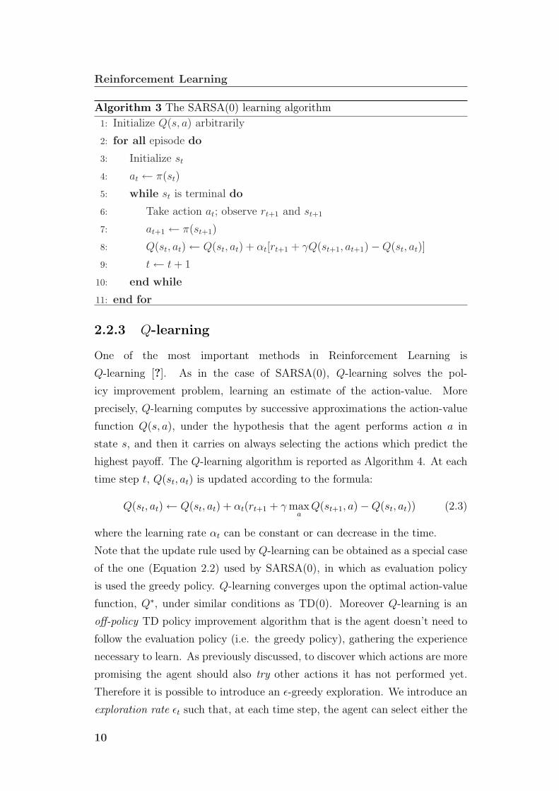
2.2.3 Q-learning
One of the most important methods in Reinforcement Learning is
Q-learning [?]. As in the case of SARSA(0), Q-learning solves the pol-
icy improvement problem, learning an estimate of the action-value. More
precisely, Q-learning computes by successive approximations the action-value
function Q(s, a), under the hypothesis that the agent performs action a in
state s, and then it carries on always selecting the actions which predict the
highest payoff. The Q-learning algorithm is reported as Algorithm 4. At each
time step t, Q(st, at) is updated according to the formula:
Q(st, at)← Q(st, at) + αt(rt+1 + γ maxa
Q(st+1, a)−Q(st, at)) (2.3)
where the learning rate αt can be constant or can decrease in the time.
Note that the update rule used by Q-learning can be obtained as a special case
of the one (Equation 2.2) used by SARSA(0), in which as evaluation policy
is used the greedy policy. Q-learning converges upon the optimal action-value
function, Q∗, under similar conditions as TD(0). Moreover Q-learning is an
off-policy TD policy improvement algorithm that is the agent doesn’t need to
follow the evaluation policy (i.e. the greedy policy), gathering the experience
necessary to learn. As previously discussed, to discover which actions are more
promising the agent should also try other actions it has not performed yet.
Therefore it is possible to introduce an ε-greedy exploration. We introduce an
exploration rate εt such that, at each time step, the agent can select either the
10

2.2 Temporal Difference Learning
Algorithm 4 The Q-learning algorithm
1: Initialize Q(s, a) arbitrarily
2: for all episode do
3: Initialize st
4: while st is terminal do
5: at ← π(st)
6: Take action at; observe rt+1 and st+1
7: Q(st, at)← Q(st, at) + αt[rt+1 + γ maxa′ Q(st+1, a′)−Q(st, at)]
8: t← t + 1
9: end while
10: end for
action which predict the highest payoff with probability 1−εt or can randomly
select another action with probability εt. Note that the exploration rate εt can
be constant or can decrease in the time.
2.2.4 Eligibility Traces
The algorithms seen so far, are 1-step temporal difference learning methods,
i.e. their updates use only information gained with immediate reward and the
estimate of successor state value. When one step learning methods are applied
to a problem, new return information is propagated back only to the previous
state. Thus, this can result in extremely slow learning in cases where credit
for visiting a particular state or taking a particular action is delayed by many
time steps. A speedup of the learning process is possible, by modifying the
return target estimate to look further ahead than the next state. How can we
use the experience collected at every single step to update estimates of many
previously visited states? First, let us define the n-step return at time t:
R(n)t = rt+1 + γrt+2 + γ2rt+3 + ... + γn−1rt+n + γnVt(st+n). (2.4)
where γ is the discount factor defined before. Instead of using the 1-step
return as target estimate, to speed up the learning process, we use a weighted
average of n-step return (with n that goes from 1 to ∞). This new target,
called λ-return is defined as:
Rλt = (1− λ)
∞∑n=1
λn−1R(n)t . (2.5)
11
Reinforcement Learning
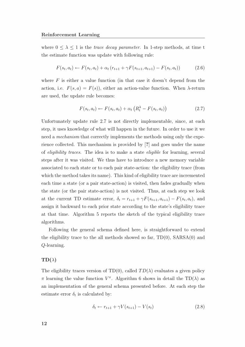
where 0 ≤ λ ≤ 1 is the trace decay parameter. In 1-step methods, at time t
the estimate function was update with following rule:
F (st, at)← F (st, at) + αt (rt+1 + γF (st+1, at+1)− F (st, at)) (2.6)
where F is either a value function (in that case it doesn’t depend from the
action, i.e. F (s, a) = F (s)), either an action-value function. When λ-return
are used, the update rule becomes:
F (st, at)← F (st, at) + αt
(Rλ
t − F (st, at))
(2.7)
Unfortunately update rule 2.7 is not directly implementable, since, at each
step, it uses knowledge of what will happen in the future. In order to use it we
need a mechanism that correctly implements the methods using only the expe-
rience collected. This mechanism is provided by [?] and goes under the name
of eligibility traces. The idea is to make a state eligible for learning, several
steps after it was visited. We thus have to introduce a new memory variable
associated to each state or to each pair state-action: the eligibility trace (from
which the method takes its name). This kind of eligibility trace are incremented
each time a state (or a pair state-action) is visited, then fades gradually when
the state (or the pair state-action) is not visited. Thus, at each step we look
at the current TD estimate error, δt = rt+1 + γF (st+1, at+1)− F (st, at), and
assign it backward to each prior state according to the state’s eligibility trace
at that time. Algorithm 5 reports the sketch of the typical eligibility trace
algorithms.
Following the general schema defined here, is straightforward to extend
the eligibility trace to the all methods showed so far, TD(0), SARSA(0) and
Q-learning.
TD(λ)
The eligibility traces version of TD(0), called TD(λ) evaluates a given policy
π learning the value function V π. Algorithm 6 shows in detail the TD(λ) as
an implementation of the general schema presented before. At each step the
estimate error δt is calculated by:
δt ← rt+1 + γV (st+1)− V (st) (2.8)
12

2.2 Temporal Difference Learning
Algorithm 5 The typical RL algorithm with elegibility trace
1: Initialize the value function arbitrarily and e(s) = 0, for all s ∈ S2: for all episode do
3: Initialize st
4: for all step of episode do
5: at ← π(st)
6: Take action at; observe rt+1 and st+1
7: δt ← difference between the target and current estimate
8: update e(st)
9: for all s ∈ S do
10: update the value function based on δt and e(s)
11: update e(s)
12: end for
13: t← t + 1
14: end for
15: end for
As result of the iteration of the TD(λ) algorithm, for each state, the eligibility
trace is updated as follows:
e(s) =
{γλe(s) + 1 if s = st,
γλe(s) otherwise(2.9)
where γ is the discount factor, and λ is the trace decay parameter defined
above.
The estimate error is, at each step, backpropagated to each state s ∈ S,
according to the eligibility trace of that state:
V (s)← V (s) + αtδte(s) (2.10)
SARSA(λ)
When using eligibility traces, SARSA(0), becomes SARSA(λ). It tries to learn
the optimal policy, evaluating a policy π and improving it gradually. Algo-
rithm 7 shows in detail the implementation of the general schema. At each
step t, estimate error is calculated by:
δt ← rt+1 + γQ(st+1, at+1)−Q(st, at) (2.11)
13

Reinforcement Learning
Algorithm 6 The TD(λ) algorithm
1: Initialize V (s) arbitrarily and e(s) = 0, for all s ∈ S2: for all episode do
3: Initialize st
4: for all step of episode do
5: at ← π(st)
6: Take action at; observe rt+1 and st+1
7: δt ← rt+1 + γV (st+1)− V (st)
8: e(st)← e(st) + 1
9: for all s ∈ S do
10: V (s)← V (s) + αtδte(s)
11: e(s)← γλe(s)
12: end for
13: t← t + 1
14: end for
15: end for
In SARSA(λ) eligibility trace are not associated to states, but to state-action
pairs. As results of one algorithm iteration, at time t eligibility trace are
updated as follows, for each state in S and for each action in A:
e(s, a) =
{γλe(s, a) + 1 if s = stand a = at,
γλe(s, a) otherwise(2.12)
Finally, at each step, the estimate error is propagated backward to each state
and action, according to their traces:
Q(s, a)← Q(s, a) + αtδte(s, a) (2.13)
Q(λ)
We’ve seen Q-learning is an off-policy method, since it learns the greedy policy
while (typically) follows a policy involving exploratory actions. For this reason
there are some problems in introducing eligibility traces. Watkins proposes
to truncate the λ-return estimate such that the rewards following off-policy
actions are removed from it [?]. Aside from this difference, Watkins Q-learning
follows the same principles of SARSA(λ), except that the eligibility traces are
14

2.2 Temporal Difference Learning
Algorithm 7 The SARSA(λ) algorithm
1: Initialize Q(s, a) arbitrarily and e(s, a) = 0, for all s ∈ S, a ∈ A2: for all episode do
3: Initialize st, at
4: while s is not terminal do
5: for all step of episode do
6: Take action at; observe rt+1 and st+1
7: at+1 ← π(st+1) . a policy derived from Q
8: δt ← rt+1 + γQ(st+1, at+1)−Q(st, at)
9: e(st, at)← e(st, at) + 1
10: for all s ∈ S, a ∈ A do
11: Q(s, a)← Q(s, a) + αtδte(s, a)
12: e(s, a)← γλe(s, a)
13: end for
14: t← t + 1
15: end for
16: end while
17: end for
set to zero whenever an exploratory action is taken. The trace update occurs
in two phases: first the traces for all state-action pairs are either decayed,
or set to 0, second the trace corresponding to the current state and action is
incremented by 1. Algorithm 8 shows the complete algorithm.
If exploratory actions are frequent, then we will lose much of the advantage
of using eligibility traces. Peng and Williams define an alternate version of
Q(λ), in which eligibility traces are not truncated, and which assumes that
all rewards are those observed under a greedy policy. The resulting method
is neither on-policy nor off-policy, and so Qt converges to a solution that is
between Qπ and Q∗. For more details on Peng and William’s Q(λ) see [?, ?].
15

Reinforcement Learning
Algorithm 8 The Watkin’s Q(λ) algorithm
1: Initialize Q(s, a) arbitrarily and e(s, a) = 0, for all s ∈ S, a ∈ A
2: for all episode do
3: Initialize st, at
4: while s is not terminal do
5: for all step of episode do
6: Take action at; observe rt+1 and st+1
7: at+1 ← π(st+1) . a policy derived from Q
8: a∗ ← argmaxbQ(st+1, b)
9: δt ← rt+1 + γQ(st+1, a∗)−Q(st, at)
10: e(st, at)← e(st, at) + 1
11: for all s ∈ S, a ∈ A do
12: Q(s, a)← Q(s, a) + αtδte(s, a)
13: if a′ = a∗ then
14: e(s, a)← γλe(s, a)
15: else
16: e(s, a)← 0
17: end if
18: end for
19: t← t + 1
20: end for
21: end while
22: end for
2.3 Curse of Dimensionality and Task decom-
position
All the RL methods presented are guardanted to converge only if they have the
states and actions represented by a table and if the number of visits for every
action-state pair stretches to infinite. In practice this means that they require
an high number of visits for every action-state pair. This is a problem because
the tabular representation have a dimension that is exponential in the number
of the variables and also in the discretization intervals of them, if the used
variables are continuous. Consequently, in general, complex problem have a
big tabular representation. In this cases there is a trade-off to consider: on
16
2.4 Summary
one hand a fine discretization permits an higher quality approximation of the
variables; from the other hand a coarse discretization can sensibly reduce the
table’s dimension. If the table’s dimension is too high there is the risk to have
action-state pairs that the agent will never visit. Instead if the discretization
is excessive there is the risk that the algorithm don’t converges to the optimal
action-value function.
A possible solution to this dilemma is to adopt a function’s approximation, but
in this case there are some problems about the convergence of the algorithm
and the optimality of the learning. Another solution is to apply the method
of the task decomposition, that is a powerful, general principle in artificial
intelligence that has been used successfully with machine learning in tasks
like, for example, the full robot soccer task [?]. Complex control tasks can
often be solved by decomposing them into hierarchies of manageable subtasks.
If learning a monolithic behavior proves infeasible, it may be possible to make
the problem tractable by decomposing it into some number of components. In
particular, if the task can be broken into independent subtasks, each subtask
can be learned separately, and combined into a complete solution [?]. More-
over with all the RL methods previously presented is not easy to insert the
a priori knowledge that we could have about the problem to solve. With the
task decomposition we could use this knowledge implicitly inserting it in the
decomposition of the task.
The decomposition procedure places another trade-off, that is the problem to
choose how many subtasks to determine: on one hand we would to individ-
uate the simplest subtasks to learn, that mean very specialized tasks; on the
other hand we don’t want to have an high number of subtasks, because this
make more complex to realize the high level controller that coordinate all this
subtasks. Therefore we must keep in mind this trade-off when we realize the
decomposition of a complex task.
2.4 Summary
We’ve seen that in Reinforcement Learning, the agent is not told what action to
take, but instead it must try the possible actions to discover which one may lead
to receive as much rewards as possible in the future. Moreover, agent actions
usually affect not only the immediate reward but also the next environment
17

Reinforcement Learning
state and, thus, also the subsequent rewards. These two characteristics, trial-
and-error search and delayed reward, are the two distinguishing features of
Reinforcement Learning. We show as temporal difference learning methods
solve RL problems starting from the simple one step algorithms. In order to
speed up the learning process through a better backpropagation of experience
collected, eligibility traces mechanism is introduced and used to extend the
TD algorithms. Finally we’ve seen how the problem of curse of dimensionality
can be solved using the technique of task decomposition.
18

Chapter 3
Machine Learning in Computer
Games
In this Chapter we give an overview of the most relevant works in the litera-
ture along with the motivations for applying Machine Learning techniques to
computer games. In the first section we introduce the problem of applying ML
to computer games focusing on the most common ML approaches to computer
games and on the advantages that it can bring to the game’s experience. Then
we focus on racing games and review the related works in the literature. Finally
we introduce the most known open source racing simulator environments.
3.1 Machine Learning in Computer Games
The area of commercial computer games has seen many advancements in re-
cent years. Hardware used in game consoles and personal computers continues
to improve, getting faster and cheaper at a dizzying pace. Computer game
developers start each new project with increased computational resources,
and a long list of interesting new features they would like to incorporate
[?]. Consequently the games have become more sophisticated, realistic and
team-oriented. At the same time they have become modifiable and are even
republished open source. However the artificial players still mostly use hard-
coded and scripted behaviors, which are executed when some special action by
the player occurs; no matter how many times the player exploits a weakness,
that weakness is never repaired. Instead of investing into more intelligent
Machine Learning in Computer Games
opponents or teammates the game industry has concentrated on multi player
games in which several humans play with or against each other. By doing this
the gameplay of such games has become even more complex by introducing
cooperation and coordination of multiple players. Thus, making it even more
challenging to develop artificial characters for such games, because they have
to play on the same level and be human-competitive without outnumbering
the human players [?].
Therefore, modern computer games offer interesting and challenging prob-
lems for artificial intelligence (AI) research. They feature dynamic, virtual
environments and very graphic representations which do not bear the prob-
lems of real world applications but still have a high practical importance.
What makes computer games even more interesting is the fact that humans
and artificial players interact in the same environment. Furthermore, data on
the behavior of human players can be collected and analyzed [?]. One of the
most compelling yet least exploited technologies is machine learning. Thus,
there is an unexplored opportunity to make computer games more interesting
and realistic, and to build entirely new genres. Such enhancements may have
applications in education and training as well, changing the way people interact
with their computers [?].
The behavior of the agents in current games is often repetitive and pre-
dictable. In most computer games, simple scripts cannot learn or adapt to
control the agents: opponents will always make the same moves and the game
quickly becomes boring. Machine learning could potentially keep computer
games interesting by allowing agents to change and adapt [?]. However, a
major problem with learning in computer games is that if behavior is allowed
to change, the game content becomes unpredictable. Agents might learn id-
iosyncratic behaviors or even not learn at all, making the gaming experience
unsatisfying. One way to avoid this problem is to train agents to perform
complex behaviors offline, and then freeze the results into the final, released
version of the game. However, although the game would be more interest-
ing, the agents still could not adapt and change in response to the tactics of
particular players [?].
20
3.1 Machine Learning in Computer Games
3.1.1 Out-Game versus In-Game Learning
In literature are defined two types of learning in computer games. In out-game
learning (OGL), game developers use ML techniques to pretrain agents that
no longer learn after the game is shipped. In contrast, in in-game learning
(IGL), agents adapt as the player interacts with them in the game; the player
can either purposefully direct the learning process or the agents can adapt
autonomously to the player’s behavior. IGL is related to the broader field of
interactive evolution, in which a user influences the direction of evolution of
e.g. art, music, etc. [?]. Most applications of ML to games have used OGL,
though the distinction may be blurred from the researcher’s perspective when
online learning methods are used for OGL. However, the difference between
OGL and IGL is important to players and marketers, and ML researchers will
frequently need to make a choice between the two [?].
In a Machine Learning Game (MLG), the player explicitly attempts to
train agents as part of IGL. MLGs are a new genre of computer games that
require powerful learning methods that can adapt during gameplay. Although
some conventional game designs include a “training” phase during which the
player accumulates resources or technologies in order to advance in levels, such
games are not MLGs because the agents are not actually adapting or learning.
Prior examples in the MLG genre include the Tamagotchi virtual pet and the
computer “God game” Black & White. In both games, the player shapes the
behavior of game agents with positive or negative feedback. It is also possible
to train agents by human example during the game, as van Lent and Laird [?]
described in their experiments with Quake II [?].
3.1.2 The Adaptivity of AI in Computer Games
Genuinely adaptive AIs will change the way in which games are played by
forcing the player to continually search for new strategies to defeat the AI,
rather than perfecting a single technique. In addition, the careful and consid-
ered use of learning makes it possible to produce smarter and more robust AIs
without the need to preempt and counter every strategy that a player might
adopt. Moreover, in-game learning can be used to adapt to conditions that
cannot be anticipated prior to the game’s release, such as the particular styles,
tastes, and preferences of individual players. For example, although a level
21

Machine Learning in Computer Games
designer can provide hints to the AI about some player’s preferences, different
players will probably have a different one. Clearly, an AI that can learn such
preferences will not only have an advantage over one that cannot, but will
appear far smarter to the player.
This section describes the two ways in which real learning and adaptation
can occur in games: the indirect and the direct one.
Indirect Adaptation The indirect adaptation extracts statistics from the
game’s world that are used by a conventional AI layer to modify an agent’s
behavior. The decision as to what statistics are extracted and their interpreta-
tion in terms of necessary changes in behavior are all made by the AI designer.
For example, a bot in an FPS can learn where it has the greatest success of
killing the player. AI can then be used to change the agent’s pathfinding to
visit those locations more often in the future, in the hope of achieving further
success. The role of the learning mechanism is thus restricted to extracting
information from the game’s world, and plays no direct part in changing the
agent’s behavior. The main disadvantage of the technique is that it requires
both the information to be learned and the changes in behavior that occur in
response to it to be defined a priori by the AI designer.
Direct Adaptation In direct adaptation, learning algorithms can be used
to adapt an agent’s behavior directly, usually by testing modifications to it
in the game world to see if it can be improved. In practice, this is done by
parameterizing the agent’s behavior in some way and using an optimization
algorithm or by modeling the problem as a MDP and using RL techniques to
search for the behaviors that offer the best performance. For example, in an
FPS, a bot might contain a rule controlling the range below which it will not
use a weapon and must switch to another one. Direct adaptation is generally
less well controlled than in the indirect case, making it difficult to test and
debug a directly adaptive agent. This increases the risk that it will discover
behaviors that exploit some limitation of the game engine (such as instability
in the physics simulation), or an unexpected maximum of the performance
measure. This effects can be minimized by carefully restricting the scope of
adaptation to a small number of aspects of the agent’s behavior, and limiting
the range of adaptation within each. The example given earlier, of adapting
22

3.2 Related Work
the behavior that controls when an AI agent in an FPS switches away from
a rocket launcher at close range, is a good example of this. The behavior
being adapted is so specific and limited that adaptation is unlikely to have
any unexpected effects elsewhere in the game. One of the major advantages
of direct adaptation, and indeed, one that often overrides the disadvantages
discussed earlier, is that direct adaptation is capable of developing completely
new behaviors. For example, it is, in principle, possible to produce a game
with no AI whatsoever, but which uses adaptivity to directly evolve rules for
controlling AI agents as the game is played. Such a system would perhaps be
the ultimate AI in the sense that:
• All the behaviors developed by the AI agents would be learned from their
experience in the game world, and would therefore be unconstrained by
the preconceptions of the AI designer.
• The evolution of the AI would be open ended in the sense that there
would be no limit to the complexity and sophistication of the rule sets,
and hence the behaviors that could evolve.
In summary, direct adaptation of behaviors offers an alternative to indirect
adaptation, which can be used when it is believed that adapting particular
aspects of an agent’s behavior is likely to be beneficial, but when too little is
known about the exact form the adaptation should take for it to be prescribed
a priori by the AI designer.
3.2 Related Work
One of the most interesting computer game’s genre for applying ML techniques
is the racing car simulations. Real-life race driving is known to be difficult for
humans, and expert human drivers use complex sequences of actions. There
are a large number of variables, some of which change stochastically and all of
which may affect the outcome. Racing well requires fast and accurate reactions,
knowledge of the car’s behavior in different environments, and various forms
of real-time planning, such as path planning and deciding when to overtake
a competitor. In other words, it requires many of the core components of
intelligence being researched within computational intelligence and robotics.
23

Machine Learning in Computer Games
The success of the recent DARPA Grand Challenge [?], where completely
autonomous real cars raced in a demanding desert environment, may be taken
as a measure of the interest in car racing within these research communities [?].
This makes “driving“ a promising domain for testing and developing Machine
Learning techniques. For all this reasons we chosen this genre of games as
testbed for ours work.
3.2.1 Racing Cars
In the academic world there are some works related to the problem of learning
to drive a car in a computer simulation using ML approaches. Zhijin Wang and
Chen Yang [?] applied with success some RL algorithms, including Actor-Critic
method, SARSA(0) and SARSA(λ), to a very simple car racing simulation.
They modeled the car as a particle on the track plane and they represented
the state of the car with only two variables: the distance of the car to the left
wall of the track and the car’s velocity. In their works they demonstrate that
the car can learn how to avoid bumping into the walls and going backwards
using only local information instead of knowing the whole track in advance.
Such robot driver is similar to a human driver and it can work on an unknown
track.
In [?] and [?] Pyeatt, Howe and Anderson realized some experiment apply-
ing RL techniques to the car racing simulator RARS. They hypothesize that
complex behaviors should be decomposed into separate behaviors resident in
separate networks, coordinated through an higher level controller. So they have
implemented a modular neural network architecture as the reactive component
of a two layer control system for the simulated car racing. The results of this
work show that with this method it is possible to obtain a control system that
is competitive with the heuristic control strategies which are supplied with
RARS.
Julian Togelius and Simon M. Lucas [?] [?] have tried to evolve different
artificial neural networks with genetic algorithm as a controllers for racing
a simulated radio-controlled car around a track. The controllers use either
egocentric (first person), Newtonian (third person) or no information (open-
loop controller) about the state of the car. For the experiments they realized
a simple simulation environment in with the car can accelerate, brake and
24
3.2 Related Work
steer along a two-dimensional track, delimited by impenetrable lines. The
results of their work is that the only controllers that is able to evolve good
racing behaviors is based on a neural network acting on egocentric inputs. In
[?] they also were able to evolve a series of controllers, based on egocentric
inputs, capable to perform good racing skills on different tracks, in some cases
also in tracks don’t seen during the learning process. Moreover they evolved
specialized controllers that race very well on a particular track, outperforming,
in some cases, a human driver.
In the commercial car racing computer games Codemasters’ Colin McRae
Rally 2.0 use a neural network to drive a rally car, thus avoiding the need to
handcraft a large and complex set of rules [?]. The AI use a standard feedfor-
ward multilayer perceptron trained with the simple aim of keeping the car to
the racing line, keeping all the others higher level functions like overtaking or
recovering from crashes separated from this core activity and hand-coded. In
the Microsoft’s Forza Motorsport all the opponent car controllers have been
trained by supervised learning of human player data [?]. The player can even
train his own ”drivatars“ to race tracks in his place, after they have acquired
his or her individual driving style.
3.2.2 Other genres
Early successes in applying ML to board games have motivated more recent
work in live-action computer games. For example, Samuel [?] trained a com-
puter to play checkers using a method similar to temporal difference learning
in the first application of machine learning to games. Since then, board games
such as tic-tac-toe [?] [?], backgammon [?], Go [?] [?] and Othello [?] have
remained popular applications of ML (see [?] for a survey). A notable exam-
ple is Blondie24, which learned checkers by playing against itself without any
built-in prior knowledge [?] [?].
Recently, interest has been growing in applying ML to other computer
game’s genres. For example, Fogel et al. [?] trained teams of tanks and robots
to fight each other using a competitive coevolution system designed for training
computer game agents. Others have trained agents to fight in first and third-
person shooter games [?] [?] [?]. An example is the work of Steffen Priesterjahn
[?] in which he successfully evolved some bot in the game Quake II that are
25
Machine Learning in Computer Games
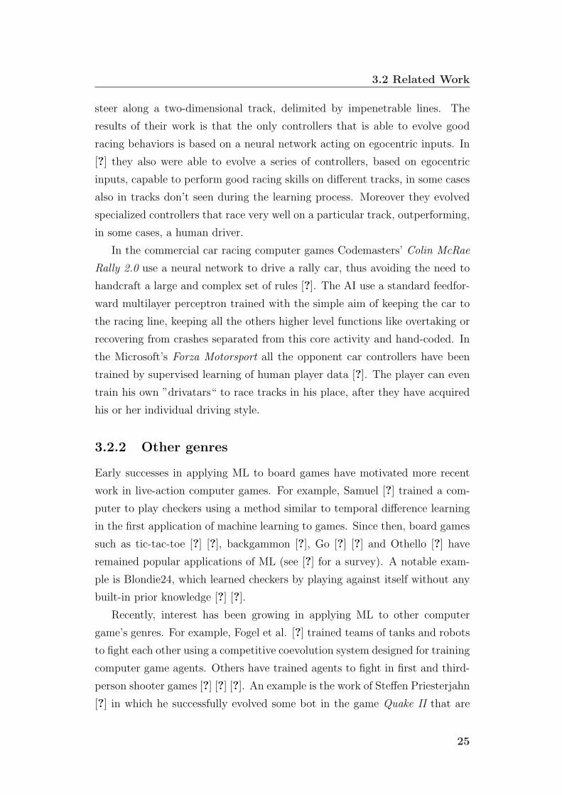
Figure 3.1: An example of two tracks of the ECR software.
able to defeat the original agents supplied by the game. ML techniques have
also been applied to other computer game genres from Pac-Man [?] to strategy
games [?] [?] [?].
3.3 Car Racing Simulators
The car racing simulation softwares available for free are the Evolutionary
Car Racing (ECR), the Robot Auto Racing Simulator (RARS) and The Open
Racing Car Simulator (TORCS). All these softwares are distributed under the
General Public License version 2 (GPL2), so the source code is available for
reuse.
3.3.1 Evolutionary Car Racing (ECR)
Evolutionary Car Racing is a simple software originally developed in Java by
Julian Togelius to apply evolutionary neural networks techniques in an envi-
ronment that simulates the behavior of small radio controlled cars [?]. The
software simulates a two-dimensional virtual environment and the tracks are
represented by a series of simple black lines (see Figure 3.1) that are impene-
trable, like a wall. Moreover the physic of the simulation is very simplified: it
models a basic wheel friction and a full elastic collision mechanism that only
partially take into account the relative angle between the car and the wall in
a collision [?] [?]. Finally, the racing environment is built to allow a single car
race, without the possibility of racing with different opponents simultaneously.
26
3.3 Car Racing Simulators
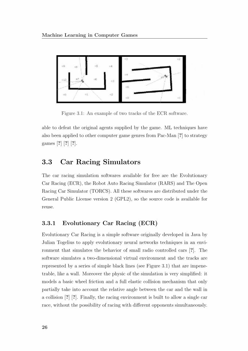
Figure 3.2: A screenshot of the game RARS.
3.3.2 RARS and TORCS
RARS is a more evolved simulation, written in C++ and explicitly realized to
allow developers to apply artificial intelligence and real-time adaptive optimal
control techniques. It simulates a complete three-dimensional environment
with a sophisticated physical model [?] (Figure 3.2 shows a screenshot of the
game). Unfortunately this project has been inactive since 2006. The place of
the RARS simulator has been taken by another one, TORCS, very similar to
RARS, but offering an higher level of quality because it’s he’s natural evolution.
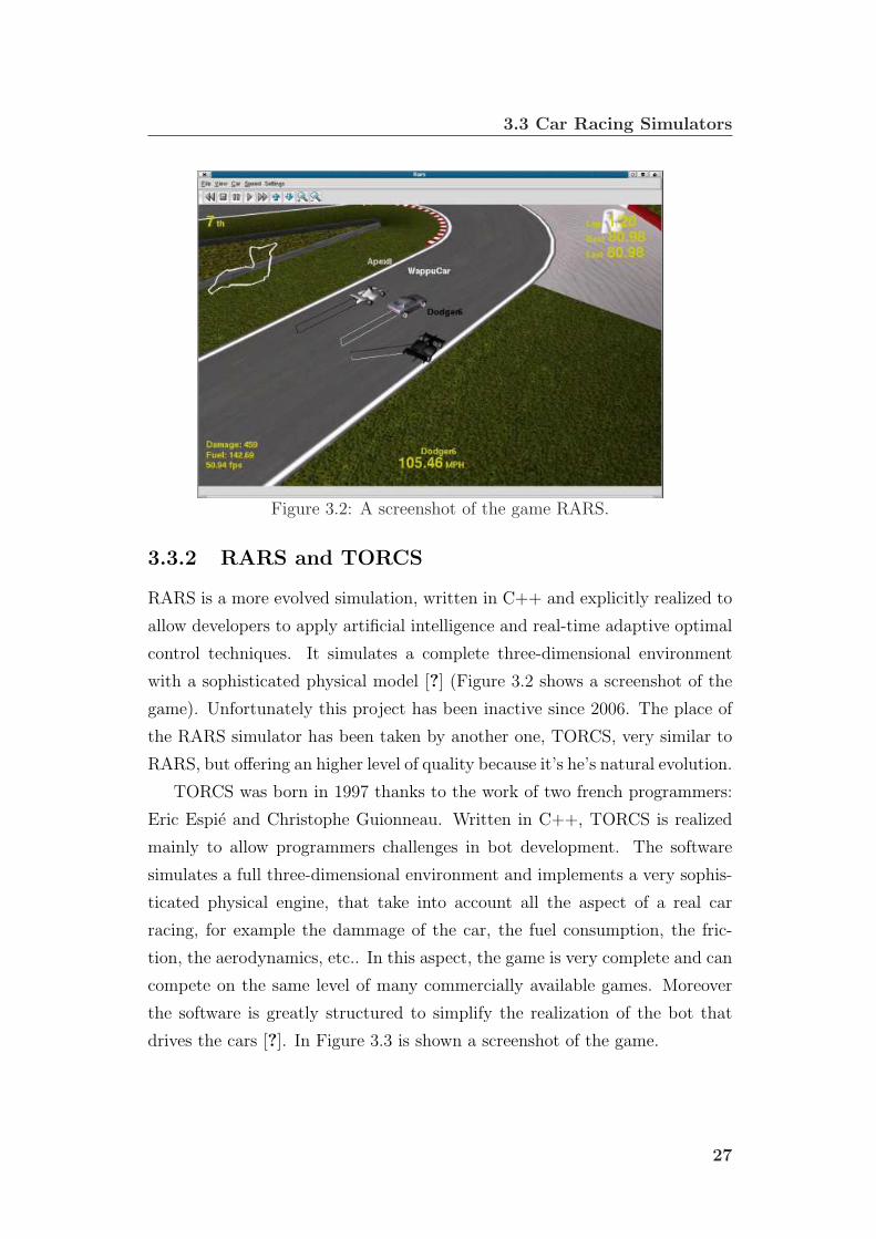
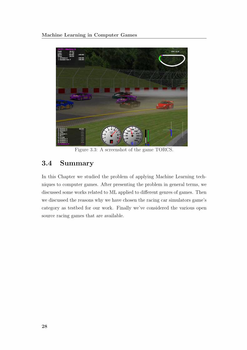
TORCS was born in 1997 thanks to the work of two french programmers:
Eric Espie and Christophe Guionneau. Written in C++, TORCS is realized
mainly to allow programmers challenges in bot development. The software
simulates a full three-dimensional environment and implements a very sophis-
ticated physical engine, that take into account all the aspect of a real car
racing, for example the dammage of the car, the fuel consumption, the fric-
tion, the aerodynamics, etc.. In this aspect, the game is very complete and can
compete on the same level of many commercially available games. Moreover
the software is greatly structured to simplify the realization of the bot that
drives the cars [?]. In Figure 3.3 is shown a screenshot of the game.
27
Machine Learning in Computer Games
Figure 3.3: A screenshot of the game TORCS.
3.4 Summary
In this Chapter we studied the problem of applying Machine Learning tech-
niques to computer games. After presenting the problem in general terms, we
discussed some works related to ML applied to different genres of games. Then
we discussed the reasons why we have chosen the racing car simulators game’s
category as testbed for our work. Finally we’ve considered the various open
source racing games that are available.
28
Chapter 4
The Open Racing Car Simulator
In this Chapter we describe in detail TORCS, the racing simulator we used
for the experimental analysis in our thesis. In the first section we present
the structure of TORCS, focusing on the simulation engine and the robot
development in TORCS. Finally we discuss the problem of interfacing the
simulation software with the Reinforcement Learning toolkit, PRLT.
4.1 TORCS
TORCS is the software chosen as the simulation environment for the experi-
ments of this work. In fact, even if it has the highest computational cost, it
presents the most interesting environment for Reinforcement Learning experi-
ments, because of the sophisticated physics of the game.
4.1.1 Simulation Engine
When TORCS is executed and the race starts, the simulation is carried out
through a sequence of calls to the simulation engine which computes the new
state of the race. Therefore, the simulation is divided into time steps of the
duration of 0.02 seconds, and at each one of these steps, each robot driving
on the circuit performs the actions suggested by its policy. The operations are
not time bounded because the simulation isn’t in real time.
The simulation engine represents each element of the car through an object
with a given set of properties. These properties are used to compute how the
car behaves to a given set of inputs from the driver (e.g. brake/accelerate) or

The Open Racing Car Simulator
from the environment (e.g. car on the grass outside the track). One of the main
limitations of the current engine is that it was conceived to compute forces in
a 2D environment and consequently it does not behave properly when the car
is moving in an uneven track or it is not perfectly parallel to the ground. All
the forces are computed as if the car was always on a leveled track with no
inclination. Furthermore, the engine doesn’t take into account tyre’s wear or
temperature, and also it does not handle properly the suspensions system and
its influence on the car’s traction.
4.1.2 Robot Development
TORCS offers the possibility to easy develop your own car controller. Infor-
mally, that piece of software is called robot, because it fits the definition usually
given for such a word: an agent that performs certain actions given a set of
inputs. In this section, the word robot will be used to refer to the software
written by the developer to control the car. The inputs come from either the
car itself or from information that can be computed given a certain set of
parameters of the car (e.g. angular velocity of the wheels). After computing
the best response to the given inputs, the robot can act on the steering wheel,
the brake or the accelerator to perform the action it thinks is best for it.
This is the complete list of the commands that the robot can use to control
the car during a race:
• Driving Commands: The commands to directly drive the car are the
steer (defined in the continuous domain [-1.0, 1.0]), the accelerator (con-
tinuous domain [0.0, 1.0]), the brake (continuous domain [0.0, 1.0]), the
clutch (continuous domain [0.0, 1.0]) and the gear selection (discrete
domain [-1, 6]).
• Pit-Stop Commands: The commands to manage the pit-stop are the
request for pit-stop, the type of the pit-stop requested (0 for refuel/repair
and 1 for “stop and go“), the amount of gasoline to refuel at the pit-stop
and the amount of damages to repair.
• Accessory Command: There is also an accessory command to switch
on/off the head lights.
30

4.2 TORCS - PRLT Interface
Developing a new robot in TORCS is the activity the game has been devel-
oped for, therefore there is an ample documentation on how to get started and
how to develop a complete controller for the game. In [?], the author explains
in great detail how to obtain a simple working robot starting from scratch, and
how to incrementally build a more complex one that is able to exploit more
complex information to perform better.
The main structure of the robots contain some fixed standard functions that
manages the initialization of the module, the race, the track representation and
the unload of the module. Moreover there is another function that is the core
of the robot and is called at every simulation timestep by the game engine,
to get the actions that the robot would to perform. This is the function that
contain all the code that evaluate the current situtation and decide what is
the best action to perform. To compute the best action at a specific time step
the robot can use a wide range of input, accessible by the car and situation
structures, that contain all the information about the own car, the track, the
opponent’s cars and the information about the race.
4.2 TORCS - PRLT Interface
To apply RL algorithms to driving tasks in TORCS we used the Polimi Rein-
forcement Learning Toolkit (PRLT) [?], a toolkit developed at Politecnico di
Milano (Dipartimento di Elettronica e Informazione), that offers several RL
algorithms and a complete framework in order to use them.
4.2.1 PRLT: An Overview
PRLT aims at providing tools to implement algorithms and run experiments
on many different environments and problems both in single and multiagent
settings. PRLT can be seen both as a stand-alone learning system and as a
learning library that can be interfaced to external systems and simulators.
The RL Agent-Environment interaction loop in PRLT As shown in
Figure 4.1, the typical Reinforcement Learning interaction loop contains sev-
eral elements: an agent, an environment, the action executed by the agent, the
31

The Open Racing Car Simulator
Figure 4.1: The RL Agent-Environment interaction loop.
Figure 4.2: The PRLT interaction loop.
state of the environment and the reward provided by the reward function of
the environment
From a high-level point of view the structure of PRLT resembles to the
RL interaction loop and it maps each element involved in the RL system to
a structure in the implementation. Roughly this mapping can be summarized
as follows (see Figure 4.2): the agent is represented by the Learning Interface,
the action and the state by the VariablesInfo, and the Reward Function by the
RewardManger.
Although all these elements are implemented in PRLT, only the Learning-
Interface is actually the element that contains all the structures needed to run
learning algorithms and that can be seen as a learning library that can be
32

4.2 TORCS - PRLT Interface
loaded also into different systems.
PRLT as a stand-alone system: the Experiment In order to put ev-
erything together PRLT uses two more elements: Experiment and toolkit. The
first one is a class that builds all the previous elements and manage them to
simulate the interaction between the Environment and the LearningInterface
and a RL experiment on several trials (i.e., episodes) with many steps each.
toolkit actually contains only the main method used to generate an object of
Experiment and to run it until it is finished.
In short, it is a double loop on trials and steps, in which at each step
the current state is obtained from the Environment and it is passed to the
LearningInterface that gives back the actions the agent wants to executed and,
unless the trial finished, they are passed to the Environment that simulates
their execution.
As it can be noticed, the Experiment has no information about the Reward-
Manager used to provide the agent the reward signal. Since the LearningIn-
terface is supposed to contain everything related to the learning process, while
the Environment could be anything and in general it is independent from a
Reinforcement Learning system, the RewardManager has been moved into the
LearningInterface that, as it will be analyzed in the next section, manages the
distribution of the reinforcement signal to the learning agent.
PRLT as a library: the LearningInterface The LearningInterface is the
core of the learning process and it is organized so that it could be used as a
library in systems different from PRLT and possibly non-learning systems (i.e.,
simulators, benchmarking frameworks, etc.). From an external point of view,
the LearningInterface provides only three methods: the first one initializes
all the learning system according to the XML configuration file passed in the
constructor and to the state space of the environment passed as parameter.
After the initialization, the LearningInterface is ready to start the learning
process according to the states visited and the actions taken by the agent and
the dynamics of the environment. The second methods determines the start
of each trial: Finally the last method is used to advance to the next learning
step. The parameters required are simply the current state of the environment
and the structure that will contain the actions the agent wants to execute.
33

The Open Racing Car Simulator
Figure 4.3: PRLT-TORCS Interface interactions.
As it can be noticed, this structure allows the LearningInterface to manage
the whole learning process without any direct interaction with the environ-
ment, whose state is provided using the VariablesInfo structure.
4.2.2 The Interface
To use the functions of the software PRLT in a TORCS robot, it’s necessary
to create an interface that must provide all the functions needed to correctly
execute the learning process. In fact, in this case we are using the PRLT
as a library, and we need a connection between the TORCS’s robot and the
LearningInterface.
Figure 4.3 shows the interactions between the various components involved
in the learning process in TORCS.
34

4.3 Summary
The state informations and the reward are passed to the LearningInterface
by the bot trough the PRLT-TORCS Interface. On the contrary the best
action to perform is passed to the bot by the LearningInterface trough the
PRLT-TORCS Interface.
4.2.3 The Used Algorithm
As we’ve seen the PRLT toolkit offers several RL algorithms. The one used
for our experiment is the Q-Learning with decreasing of parameters, that is
implemented in PRLT following the description of the algorithm discussed in
Chapter 2. In particular we use a version of Q-Learning with this decreasing
function of the learning rate parameter is:
αt(s, a) =α0
1 + δαnt(s, a)(4.1)
where αt(s, a) is the value of the learning rate for the action-state pair (s, a)
at time t, α0 is the initial learning rate, δα is the costant decreasing rate of α
and nt(s, a) is the number of visits of the algorithm to the action-state pair
(s, a) at time t.
Moreover we use an ε-greedy exploration policy with this decreasing function
for the exploration rate:
εN =ε0
1 + δεN(4.2)
where εN is the value of exploration when the algorithm is at the nth
learning episode, ε0 is the initial exploration rate, δε is the costant decreasing
rate for ε and N is the number of learning episodes elapsed.
4.3 Summary
In this Chapter we’ve discussed the reasons why TORCS was our preferred
choice. In the first section we presented a detailed description of TORCS: first
of all we analyzed the simulation engine of the game, explaining how it works
and what are its main limitation. Then we discussed the problem of interfacing
TORCS with the PRLT learning system, that is used in this work to apply
35

The Open Racing Car Simulator
the RL methods in the simulation. Finally we introduced the details of the
RL algorithm used for the experiments in our work.
36

Chapter 5
Learning to drive
In this Chapter we propose a task decomposition for the driving problem and
the experimental setting used in the thesis. In the first section we discuss how
our work is related with the existing works in literature and the type of prob-
lems we want to solve with ML, and we propose a possible task decomposition
for the problem of driving a car in the chosen simulated environment. Finally
we introduce the first simple task considered, gear shifting, and the related
experimental analysis.
5.1 The problem of driving a car
As we seen in Section 3.2.1 we choose the category of the simulated car racing
as testbed for the realization of this work. The problem of driving a car in
a sophisticated computer simulation like TORCS is a very difficult task, also
for an expert human driver or player: the amount of informations that must
be taken into account is remarkable and there is the need of adapting to dif-
ferent circumstances. Moreover depending on the current situation there are
some informations that are more relevant than others, or informations that are
unimportant. For these reasons is difficult to directly learn a complete driving
policy using ML techniques. Therefore, we decided to use the task decomposi-
tion to obtain a number of simpler subtasks that compose the complete drive
behavior.
As discussed in 3.1 there are two different type of learning that can be
applied to computer games, the out-game and the in-game. One of the aim
of this work is to learn some tasks using an OGL technique to obtain a static
Learning to drive
policy that can be used later in the game. Learning by OGL allow us to find
a policy for a certain task without the need to write an hand coded one, that
require to evaluate in advance all the possible situations in which a player could
be found during the game and also which are the best actions to perform in
every state.
The other aim of the work is to verify if it’s possible to dynamically adapt a
policy, learned with OGL, during the game, using an IGL. In fact the static
policy learned by OGL have the inconvenience that it may perform badly if
some variables that influence the task changes in the environment. Moreover
this policy could not be optimal in all the situations. With IGL is possible to
adapt the policy to some environment’s changes or to the player’s preferences,
making it more flexible and challenging.
In this work we want to solve some problems of driving using RL, because
most of this subtasks, e.g. steering or gear shifting, can be modelled as an MDP
problem. In fact, the value of the variables of the environment can be used to
determine the states, the bot represents the agent, that can performs a certain
action and it is possible to generate a reward depending on the state of the en-
vironment and the action performed by the bot. If we apply a discretization to
the variables involved in the decision process that are continuous in the game,
we can also model this problems as finite MDP. Moreover the RL techniques
have the advantage that there isn’t the need to know a priori which are the
best actions in every state: we just need to define the reward function and,
therefore, we need to know in advance just which are the negative situations
and the goal we want to reach. Finally RL adapts to an on-line paradigm,
making it easy to pass from OGL to IGL.
5.2 Task decomposition for the driving prob-
lem
In this section we propose a task decomposition for the complex task of driving
a car in the TORCS racing car simulation environment. Applying the princi-
ples of task decomposition discussed in Section 2.3 is possible to determine a
number of simpler subtasks like steering, accelerating and braking that can be
combined together to obtain a complete car driver.
38

5.2 Task decomposition for the driving problem
The Figure 5.1 shows the task decomposition proposed, represented by the
gray boxes. We divide the subtasks into four level of decisions, based on the
type of decision itself. The white boxes, instead, represents the input used in
each level.
The four levels of decisions are divided in the following way:
• strategy level (3): this level include the more complex type of decisions,
that is the decisions that require an high level analysis of the current
situation and an high number of varibales. For example the task of de-
ciding the overtake strategy must consider if there is the real opportunity
of surpass and, if it is the case, how to accomplish this task.
• planning level (2): this level include the tasks that plans the current
desired speed and trajectory on the track. These decisions are clearly
dependent on the higher level decisions taken at the strategy level: for
example the current trajectory must be modified if we decide to overtake
an opponent.
• control level (1): this level include some low level control tasks, in par-
ticular the Antilock Braking System (ABS) and the Acceleration Slip
Regulation (ASR) system and the collision avoidance.
• execution level (0): the last level include the tasks that execute all the
commands that directly control the car, e.g the value of the brake’s pres-
sure to apply. The value of these commands are assigned in consequence
of the decisions taken by the higher levels.
For simplicity we group all the possible input in three principal group,
because the real number of all the possible data are very high. The groups
are:
• Car Informations: this group contain all the data relative to the own
car, like engine’s RPM, current speed, wheel’s angular velocity, amount
of fuel, current gear, brake pressure, etc.
• Track Informations: at this group pertains all the data relative to the
track, like friction’s coefficient, length, height, width, turn radius, etc..
39
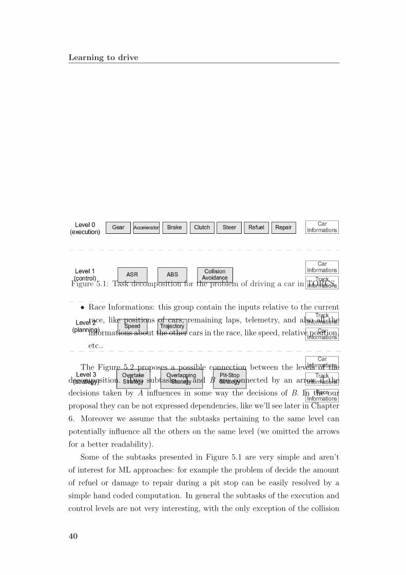
Learning to drive
Figure 5.1: Task decomposition for the problem of driving a car in TORCS.
• Race Informations: this group contain the inputs relative to the current
race, like positions of cars, remaining laps, telemetry, and also all the
informations about the other cars in the race, like speed, relative position,
etc..
The Figure 5.2 proposes a possible connection between the levels of the
decomposition. Two subtasks, A and B are connected by an arrow if the
decisions taken by A influences in some way the decisions of B. In the our
proposal they can be not expressed dependencies, like we’ll see later in Chapter
6. Moreover we assume that the subtasks pertaining to the same level can
potentially influence all the others on the same level (we omitted the arrows
for a better readability).
Some of the subtasks presented in Figure 5.1 are very simple and aren’t
of interest for ML approaches: for example the problem of decide the amount
of refuel or damage to repair during a pit stop can be easily resolved by a
simple hand coded computation. In general the subtasks of the execution and
control levels are not very interesting, with the only exception of the collision
40
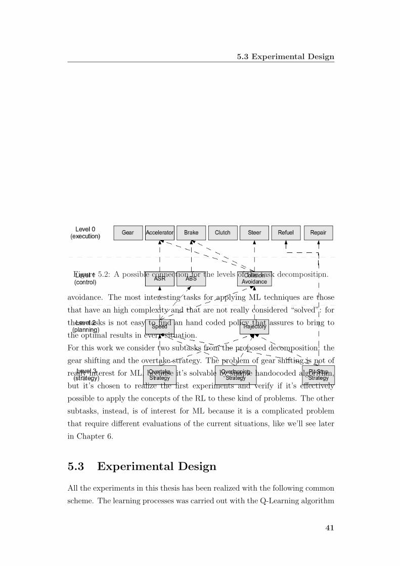
5.3 Experimental Design
Figure 5.2: A possible connection for the levels of the task decomposition.
avoidance. The most interesting tasks for applying ML techniques are those
that have an high complexity and that are not really considered “solved”: for
these tasks is not easy to find an hand coded policy that assures to bring to
the optimal results in every situation.
For this work we consider two subtasks from the proposed decomposition: the
gear shifting and the overtake strategy. The problem of gear shifting is not of
really interest for ML, because it’s solvable by simple handocoded algorithm,
but it’s chosen to realize the first experiments and verify if it’s effectively
possible to apply the concepts of the RL to these kind of problems. The other
subtasks, instead, is of interest for ML because it is a complicated problem
that require different evaluations of the current situations, like we’ll see later
in Chapter 6.
5.3 Experimental Design
All the experiments in this thesis has been realized with the following common
scheme. The learning processes was carried out with the Q-Learning algorithm
41

Learning to drive
using the PRLT toolkit: for every experiment we found a suitable parameter
setting for α0, γ, δα, ε0 and δε, and also a convenient number of episodes to
stop the learning process.
As result of the learning process is reported the learning curve, that is a moving
average of the reward collected by the agent during the learning episodes. We
also compared such learning curve with the average reward collected by an
agent that follows the handocoded policy supplied with a TORCS’s bot.
In addition, we also evaluated the learned policy by measuring one or more
physics variables relevant for the task considered, e.g. the maximum speed.
Such evaluation was carried out applying the learned policy on a certain num-
ber of episodes, without exploration and with the random starts disabled,
where used during the learning. Also in this case we compared such evaluation
with the one relative to the reference handcoded policy.
Finally we applied to these measured variables the Wilcoxon’s rank-sum test,
in order to see if the differences between the two compared policies are statis-
tically significant.
5.4 A simple Task: gears shifting
To start our work we select a simple subtasks from the previously discussed
decomposition, the gear shifting. In Figure 5.3 we show the subtasks and the
inputs involved in this problem.
As you can see the learning process is divided in two parts, the first related to
the gear changing during an acceleration and the second during a deceleration.
This division is made because the goal is different in the two cases: during
acceleration we want to decide how and when to shift the gears to obtain the
maximum acceleration; instead during breaking we want to change gears in
a way that help in the best way the braking system to obtain the maximum
deceleration. Then these two policy are then merged by an higher level control,
named Preprocessing in Figure 5.3, that decide when to switch from a policy
to the other, obtaining a complete gear shifting policy.
42

5.4 A simple Task: gears shifting
Figure 5.3: Subtasks involved in the gear shifting problem.
5.4.1 Problem definition
To successfully learn a policy for the task of shifting gears driving a car, we
must define which are the relevant data involved in this decision process. In
general we decide to shift the gear up or down considering the rotations per
minute of the engine, the actual gear and the fact that we want to accelerate,
decelerate or maintain his current speed. We consider these three elements as
inputs for the learning process. Moreover we define the output of the learning
system, that must be interpreted by the driver as the next action to perform.
Finally we also defined the reward function and the quantification of the control
time.
Gear shifting during an acceleration
The learning episode starts with the car completely stopped on a long straight.
Then the car accelerates along this straight, and the learning episode ends when
the car have reached a determined distance of 1500 meters.
A reasonable control time step is defined as 25 TORCS’s simulation time step,
corresponding to 0.5 real seconds in the simulated environment (each simula-
tion time step correspond to 0.02 real seconds).
When you are accelerating the input that identify if you are in an acceleration
state or in a deceleration one, can be eliminated. In fact this information is
43

Learning to drive
implicitly known by the driver and never change during the decision process.
So the input that defines the states of the learning process for this case are the
engine’s RPM, defined in the discrete domain [0, 10500], and the actual gear,
defined in the discrete domain [-1, 6]. To limit the space of states the engine’s
RPM values are divided into six groups, everyone of which is considered a state
of this variable: { [0 4000), [4000 6000), [6000 7000), [7000 8000), [8000 9000),
[9000 10500] }. Note also that the gear -1 correspond to the reverse gear and
the gear 0 correspond to the neutral.
The output of the learning system is defined as the gear shifting action to
perform, defined in the discrete domani [-1, 1], and it’s interpreted in this way:
shift down if the value is -1, shift up if the value is 1 and don’t shift if it’s 0.
The reward passed to the learning system at time t, rt, is defined as the vari-
ation between the speed at the current control time step, vt, and the speed at
the previous one, vt−1:
rt = vt − vt−1 (5.1)
Note that the reward is positive if the speed increases and negative if it
decreases.
Gear shifting during a deceleration
The learning episode starts with the car driving at the maximum speed on a
long straight. Then the car starts braking and the learning episode ends when
the car is completely stopped on the track.
For this case the selected control time step is smaller and is defined as 5
TORCS’s simulation time step, corresponding to 0.1 real seconds in the sim-
ulated environment. This choice is done because the process of stopping a car
is faster then accelerating and so there is a smaller time to decide what action
to perform.
Also in this case the input that identify if you are in an acceleration state or
in a deceleration one can be eliminated: it never change during the learning
episode. So the inputs that defines the states of the learning process for this
case are the same of the previous task, the engine’s RPM and the actual gear,
both defined in the same domain of the previous acceleration case.
Also the output of the learning system is defined and interpreted as in the
44

5.4 A simple Task: gears shifting
previous case.
The reward passed to the learning system at time t, rt, is defined as the varia-
tion between the speed at the previous control time step, vt−1, and the speed
at the current one, vt:In this case it’s positive if the speed decreases:
rt = vt−1 − vt (5.2)
In this case the reward is positive if the speed decreases and negative if it’s
decreases.
Merging acceleration and deceleration cases together
Now we take into account both the situation of acceleration and deceleration
to obtain a unified policy of gear shifting, valid in any possible situation of a
race along a track. To realize such policy we need to distinguish among three
possible situations: car is accelerating, car is decelerating or car is maintaining
a constant speed. So, in this case, we introduce the third input variable, that
we call acceleration/deceleration state, that change it’s value every time the
car change it’s acceleration behavior (for example when it change from an
acceleration phase to a braking one). In detail the system constantly check
the activity of the accelerator and brake pedals: is the accelerator is pushed
for at least 5 TORCS’s time step the acceleration/deceleration variable is set
to 1, if for at least the same time is pushed the brake pedal then the variable
is set to -1, and in the other cases it is set to 0.
The preprocessing unit evaluate the state of the acceleration/deceleration vari-
able and decide if it must apply the policy learned for the acceleration case or
the one learned for the deceleration. In the case that the car is maintaining
a fixed speed the preprocessing unit decide autonomously to don’t shift the
gear.
The other inputs that defines the states of the decision process for this task are
the the same as in the two previous cases: the engine’s RPM and the current
gear.
The control time is differentiated for acceleration and deceleration states: dur-
ing acceleration it’s set to 25 simulation time steps (0.5 real seconds) and
during deceleration it’s set to 5 time steps (0.1 real seconds).
45

Learning to drive
4.5
5
5.5
6
6.5
0 1000 2000 3000 4000 5000
Ave
rage
Rew
ard
Episodes
Q-LearningHandcoded
Figure 5.4: Handcoded vs Learning Policy during acceleration.
5.4.2 Experimental results
Gear shifting during an acceleration
The Q-Learning algorithm in this experiment was setup with these parameters:
α0 = 0.5, γ = 0.4, δα = 0.05, ε0 = 0.5, δε = 0.005. The algorithm has been
stopped after 5000 episodes.
The gear shifting policy learned is reasonable: the learned policy never inserts
the reverse gear and never shifts down. We can assert that the algorithm has
produced a good policy. Figure 5.4 show the graph of the average reward
(mobile averaged over a windows of 100 episodes) during the learning process
compared with the reference handcoded policy, used by the bot supplied with
TORCS.
Moreover in Table 5.1 we compare the performances of the learned and
handcoded policy. Two measures are used for the comparison: the first one is
the time (in seconds) in which the car reach the goal, that is the time elapsed
to cover the 1500 meters of each episodes; the second one is the speed (in
kilometers per hour) that the car have at the end of an episode. Both the
measures are averaged over 1000 episodes executed in exploitation mode. The
46

5.4 A simple Task: gears shifting
Policy Average Time to Goal Average Max Speed
Learned 25.587 ±0.53879 284.644 ±1.53
Handcoded 25.1648 ±0.54453 284.711 ±1.52104
Table 5.1: Handcoded vs Learned Policy Performances - Gear shifting during
acceleration
Wilcoxon’s rank-sum test have reported a statistical significance of the data
at the 99% level. As you can see from these results, the learned policy have
similar performances with respect to the handocoded one.
Gear shifting during a deceleration
The Q-Learning algorithm in this experiment was setup with these parameters:
α0 = 0.5, γ = 0.4, δα = 0.05, ε0 = 0.5, δε = 0.005. The algorithm has been
stopped after 5000 episodes.
Also in this case the learned gear shifting policy is reasonable: the car starts
driving on the track at the maximum speed with the last gear inserted, then
starts to brake and the policy maintains the same gear until a certain RPM
engine’s regime was reached. The learned policy takes advantage of the motor
brake to reach the goal of completely stopping the car as soon as possible.
Also in this case we can assert that the algorithm has produced a reasonable
policy. Figure 5.5 show the graph of the average reward (mobile averaged over
a windows of 100 episodes) during the learning process compared with the
reference handcoded policy, used by the bot supplied with TORCS.
In Table 5.2 we compare the performances of the learned and handcoded
policy. In this case we use only the measure of the average time (expressed
in seconds) in which the car reach the goal, that is the time elapsed from
the moment in which the car starts to brake and the moment in which it’s
completely stopped. The measures are averaged over 1000 episodes, executed
in exploitation mode. The Wilcoxon’s rank-sum test have reported a statistical
significance of the data at the 99% level. Also in this case the performances of
the two policies are very similar.
47
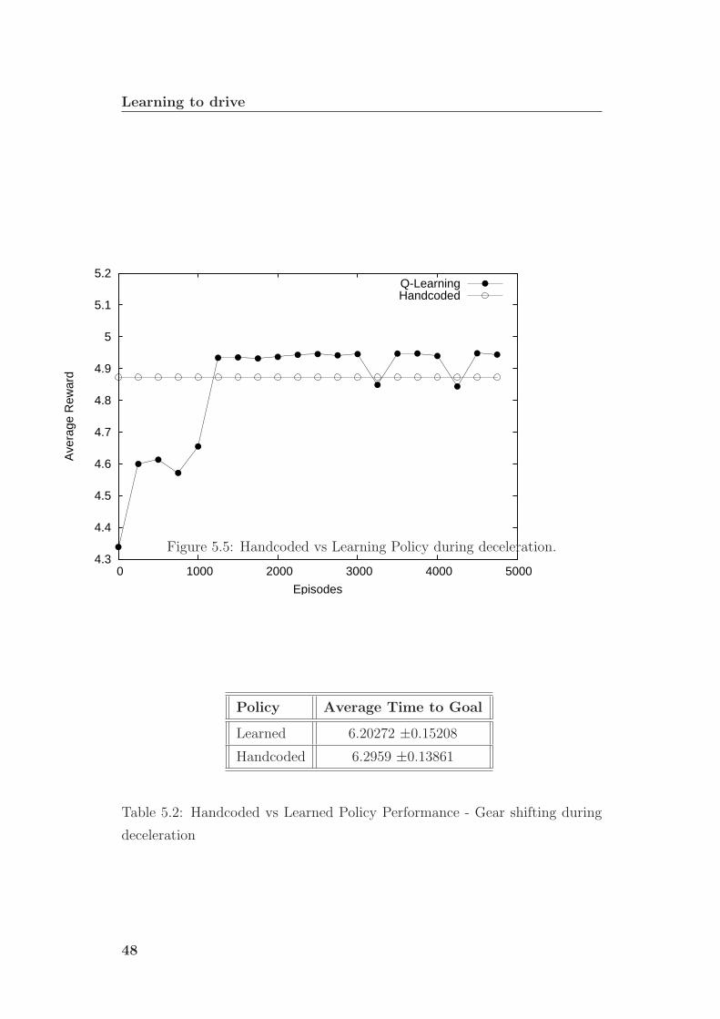
Learning to drive
4.3
4.4
4.5
4.6
4.7
4.8
4.9
5
5.1
5.2
0 1000 2000 3000 4000 5000
Ave
rage
Rew
ard
Episodes
Q-LearningHandcoded
Figure 5.5: Handcoded vs Learning Policy during deceleration.
Policy Average Time to Goal
Learned 6.20272 ±0.15208
Handcoded 6.2959 ±0.13861
Table 5.2: Handcoded vs Learned Policy Performance - Gear shifting during
deceleration
48

5.5 Summary
Policy Average Lap Time
Learned 89.0842 ±0.71239
Handcoded 89.1978 ±0.68262
Table 5.3: Handcoded vs Learned Policy Performance - Gear shifting during
a race
Merging acceleration and deceleration cases together
In this case we haven’t made a new learning procedure. Instead, we merged
the two policy obtained in the previous experiments with a module that de-
cide at an higher level which policy to use, accordingly with the accelera-
tion/deceleration input variable. The experiment is executed on different sit-
uations with respect to the the ones used to learn the two merged policies.
In fact in the previous experiments we learned the gear shifting policy during
acceleration and deceleration on a straight and with a stationary episode’s
start condition. In this experiment, instead, the car run over a different track,
when the episodes can starts from different conditions and can have variable
duration. Table 5.3 shows the performances of the learned and handcoded
policies. In this case we use the average lap time as measure of performance
(the measures are averaged over 100 laps). The Wilcoxon’s rank-sum test have
reported a statistical significance of the data at the 99% level. As you can see,
even if the learned policy is applied to a new type of situation, the obtained
performance is a little higher with respect to the one of the handcoded policy.
5.5 Summary
In this Chapter we presented the context in which is placed our work, and we
applied the principles of the task decomposition to the complex task of driving
a car, presenting a possible decomposition. Then we analyzed the first simple
subtask considered, the gear shifting: we’ve seen that is possible to learn this
task with Q-Learning and that this algorithm was capable of exploit a good
gear shifting policy.
49


Chapter 6
Learning to overtake
In this Chapter we present an higher level task, the overtaking strategy and the
experiments that aim to learn a policy for this problem. In the first section
we show that this task can be further decomposed into two subtasks: the
Trajectory Selection and the Braking Delay, everyone of which corresponds to
a different behavior for overtaking. Then we describe in detail the Trajectory
Selection subtask and we show that it can be solved with Q-Learning. In ad-
dition we show that our approach can be extended to different environmental
conditions, i.e. different versions of the aerodynamic model and different op-
ponent’s behaviors. Then we describe the second subtask, the Braking Delay.
Firstly we apply the Q-Learning algorithm for learning a good policy for this
subtasks and then we show that the learned policy can be adapted to a change
in the environment during the learning process.
6.1 The Overtake Strategy
In this chapter we focused on a more complex task: the problem of overtaking
an opponent in a race. This task belowes to the strategy level according to
the decomposition proposed in Section 5.2. Because of the complexity of this
task, we further decomposed it in this two subtasks (as shown in Figure 6.1):
the trajectory selection and the braking delay. This division is made because
we individuate two different behavior for overtaking: the first one modifies the
current desired trajectory to accomplish the surpass avoiding to go off road or
to collide with the opponent, the second one influences the braking policy in
the particular situation in which we approach a turn during the overtake of
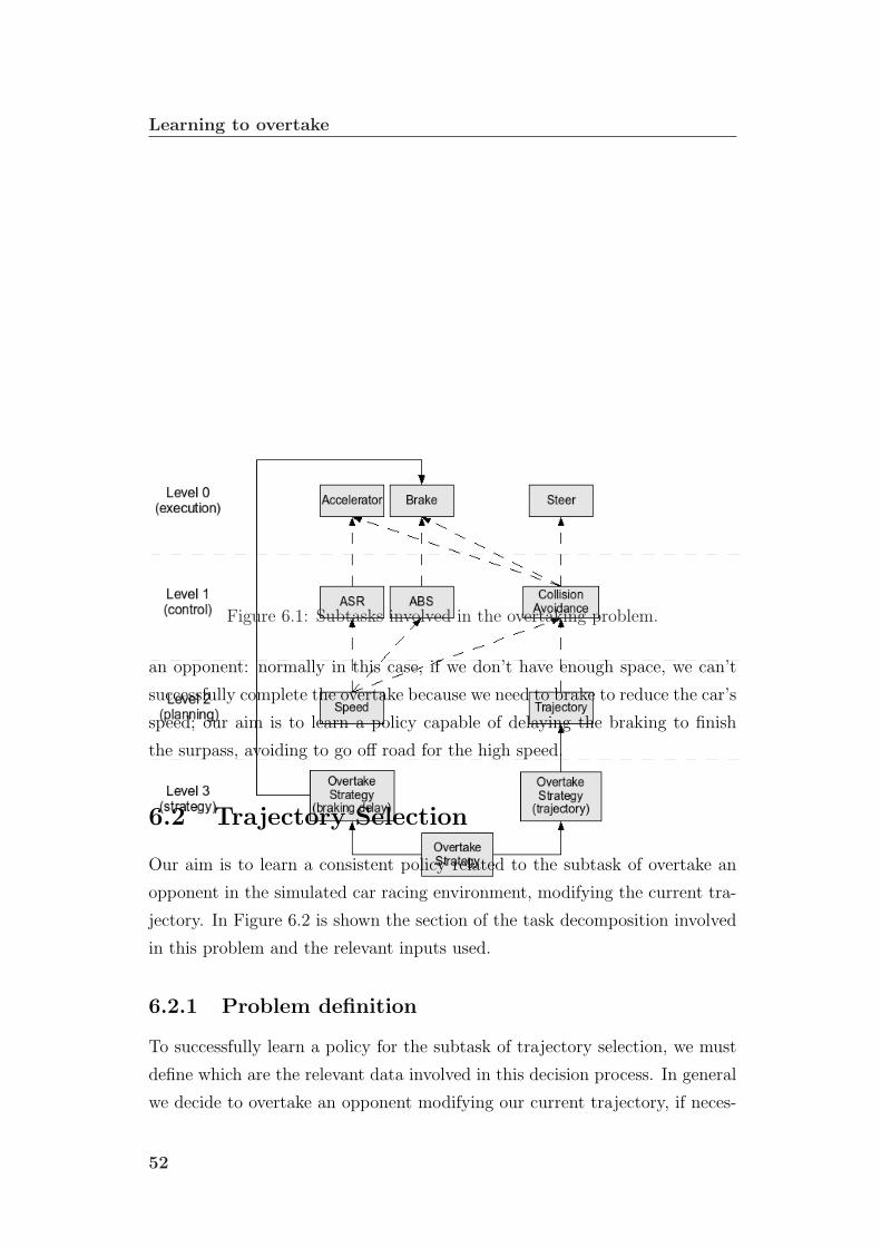
Learning to overtake
Figure 6.1: Subtasks involved in the overtaking problem.
an opponent: normally in this case, if we don’t have enough space, we can’t
successfully complete the overtake because we need to brake to reduce the car’s
speed; our aim is to learn a policy capable of delaying the braking to finish
the surpass, avoiding to go off road for the high speed.
6.2 Trajectory Selection
Our aim is to learn a consistent policy related to the subtask of overtake an
opponent in the simulated car racing environment, modifying the current tra-
jectory. In Figure 6.2 is shown the section of the task decomposition involved
in this problem and the relevant inputs used.
6.2.1 Problem definition
To successfully learn a policy for the subtask of trajectory selection, we must
define which are the relevant data involved in this decision process. In general
we decide to overtake an opponent modifying our current trajectory, if neces-
52

6.2 Trajectory Selection
Figure 6.2: Outline of the Trajectory Selection problem.
sary, taking into account some distances like the frontal and lateral distance
from the opponent and how much fast we are approaching the car to overtake.
These values are important to calculate a trajectory that allows the driver to
overtake the opponent avoiding a collision. Moreover the driver must consider
his distance from the edges of the track, in order to avoid to go off road.
Therefore the input used as state variables for the learning process are: the
opponent’s frontal distance, defined in the continuous domain [0, 200], the
opponent’s lateral distance, defined in the continuous domain [-25, 25], the
track’s edge distance, defined in the continuous domain [-10, 10] and the delta
speed, defined in the continuous domain [-300, 300].
We also define the output of the learning system defined in the discrete domain
[-1, 1], that must be interpreted by the driver as the next action to perform:
if the value of the output is -1, the agent adds an offset of one meter on the
left to the current target trajectory, if the value is 1 he adds an offset of one
meter on the right to the current target trajectory, and if the value is 0 the
agent don’t modify the current trajectory.
In this experiment each learning episode begin with a random condition. The
random start generates two conditions: a frontal distance value and a lateral
distance one. The learning episode starts with the car positioned in these
random generated points relative to the opponent’s car. The episode ends
when the car go off road, collides with the other car or when it reaches the
53

Learning to overtake
goal. The goal is to have a distance of 0 meters with respect of the opponent,
that means that the overtake is successfully accomplished. The opponent’s car
is set up to drive at the center of the track, maintaining a fixed speed of 150
Km/h.
Moreover this is the defined reward function for this subtask:
rt =
1 if the goal was reached
−1 if the car go off road or collides with the opponent
0 otherwise
(6.1)
To limit the space of states the domains of all the input variables are
discretized and divided into groups, everyone of which is considered a discrete
state for the corresponding variable. In particular the opponent’s frontal dis-
tance is discretized as { [0 10) [10 20) [20 30) [30 50) [50 100) [100 200] }, the
opponent’s lateral distance as { [-25 -15) [-15 -5) [-5 -3) [-3 -1) [-1 0) [0 1) [1
3) [3 5) [5 15) [15 25] }, the track’s edge distance as { [-10 -5) [-5 -2) [-2 -1) [-1
0) [0 1) [1 2) [2 5) [5 10] } and finally the delta speed is discretized as { [-300
0) [0 30) [30 60) [60 90) [90 120) [120 150) [150 200) [200 250) [250 300] }.The first three inputs are measured in meters: the opponent’s lateral distance
and the track’s edge distance have a negative value when the driver is located
at the right side with respect of the opponent’s car and in the right side of the
track with respect to the middle line, respectively. This allow the driver to
distinguish between the two symmetric respective situations. The information
of how much fast the driver is approaching the opponent, represented by the
delta speed variable, is expressed as the difference between the speed of the car
that is overtaking and the car that is in order to be surpassed (this value is
measured in kilometers per hour). The value of this state variable is negative
when the driver have a lower speed than the opponent.
Finally, the control time chosen for this subtask is of 10 TORCS’s simulation
time steps, corresponding to 0.2 real seconds in the simulated environment.
6.2.2 Experimental results
The parameter setting of the Q-Learning algorithm in this experiment is: α0 =
0.5, γ = 0.95, δα = 0.05, ε0 = 0.5, δε = 0.0005. The algorithm has been stopped
after 11000 episodes.
54

6.2 Trajectory Selection
-0.01
-0.005
0
0.005
0.01
0.015
0.02
0 2000 4000 6000 8000 10000
Ave
rage
Rew
ard
Episodes
Q-LearningHandcoded
Figure 6.3: Handcoded vs Learning Policy for Trajectory Selection subtask.
The car has learned a good overtake strategy: the car decides to surpass
the opponent from the right or left side according to the random start position.
The car correctly learn to avoid the collisions with the opponent and also to
stay on the track and only in rare cases it commits an error.
Figure 6.3 shows the value of the average reward for the learning policy com-
pared with the reference handcoded policy, obtained with a mobile average.
You notice that the learned policy exploits a slightly higher value of average
reward with respect to the handcoded one. This improvement can be explained
analyzing the aerodynamic model of the game: the simulation engine imple-
ment an approximated drag effect behind the cars, producing a decrement of
the aerodynamic drag with the geometry of a cone, as shown in Figure 6.4.
This allows the Q-Learning algorithm to exploit a better policy with respect
to the reference one, that don’t take into account of the aerodynamic model
in the overtaking.
In addition the learned policy generalizes well in turns: the car learns to
nearly always correctly manage the trajectory also if it meets a turn during an
overtake episode.
In Table 6.1 we compare the performances of the learned and handcoded
55

Learning to overtake
-8-4
0 4
8 0 30 60 90 120 150 180
0
1000
2000
3000
4000
5000
Aerodynamic Friction
Lateral Distance
Frontal Distance
Aerodynamic Friction
Figure 6.4: Aerodynamic Cone (20 degrees).
Policy Average Time to Goal Average Max Speed
Learned 15.1187 ±1.08348 205.572 ±1.66118
Handcoded 15.442 ±1.1101 197.444 ±1.91045
Table 6.1: Handcoded vs Learned Policy Performances - Trajectory Selection
policy. Two measures are used for the comparison: the first one is the time
(in seconds) necessary for reaching the goal, that is the time elapsed from the
start of an episode to the accomplishment of the overtake; the second one is the
maximum speed (expressed in kilometers per hour) that the car have reached
during the overtake. Both the measures are averaged over 200 episodes. The
Wilcoxon’s rank-sum test have reported a statistical significance of the data
at the 99% level. As you can see from these results, the learned policy have
an higher performances with respect to the handocoded one.
56

6.2 Trajectory Selection
-8-4
0 4
8 0 30 60 90 120 150 180
0
1000
2000
3000
4000
5000
Aerodynamic Friction
Lateral Distance
Frontal Distance
Aerodynamic Friction
Figure 6.5: Narrow Aerodynamic Cone (4.8 degrees).
6.2.3 Adapting the Trajectory Selection to different
conditions
Now we want to check if we can obtain good results making more difficult to
take advantage of the aerodynamic cone. Therefore we modified the aerody-
namic model of the game to create a different version of the cone behind the
cars. In Figure 6.5 is shown the new used cone: it’s more narrow than the
previous one (4.8 degrees of amplitude against the 20 degrees of the original
one) and have a different decreasing rate of the aerodynamic drag, that is
distributed for a longer distance behind the opponent car.
The parameter setting of the Q-Learning algorithm used in this experiment is
the same used in the previous one. Also in this case the algorithm has been
stopped after 11000 episodes.
In Figure 6.6 you can see the results of the new experiment, comparing
the average reward obtained by the new learning policy and the handcoded
one. As you can notice in this case the learned policy have exploited advantage
with respect to the reference policy, demostrating that the learning system has
taken advantage of the new aerodynamic effects.
57

Learning to overtake
-0.015
-0.01
-0.005
0
0.005
0.01
0.015
0.02
0.025
0 2000 4000 6000 8000 10000
Ave
rage
Rew
ard
Episodes
Q-LearningHandcoded
Figure 6.6: Handcoded vs Learning Policy for Trajectory Selection subtask
with narrow Aerodynamic Cone.
In Table 6.2 we compare the performances of the learned and handcoded
policy. The two measures are the same used for the previous experiment: the
time (in seconds) necessary for reaching the goal and the maximum speed (in
kilometers per hour) that the car have reached during the overtake. Both
the measures are averaged over 200 episodes. The Wilcoxon’s rank-sum test
have reported a statistical significance of the data at the 99% level. As you
can see from these results, also in this case the learned policy have an higher
performances with respect to the handocoded one.
Changing the opponent’s behavior
Now we try to learn the subtask of trajectory selection in a more complex
situation: we repeat the previous experiment with a modified opponent’s be-
havior (using the narrow aerodynamic cone). In the previous experiments the
opponent’s car was setup to drive at the center of the track, maintaining a
fixed speed of 150 Km/h; now, instead, the opponent randomly change its
position over the track and its velocity, between 150 and 180 Km/h, every
58

6.3 Braking Delay
Policy Average Time to Goal Average Max Speed
Learned 14.7873 ±1.08037 198.98 ±4.83283
Handcoded 16.051 ±1.21126 190.042 ±1.90178
Table 6.2: Handcoded vs Learned Policy Performances - Trajectory Selection
with narrow Aerodynamic Cone
three seconds.
The parameter setting of the Q-Learning algorithm used in this experiment is
the same used in the previous one. Also in this case the algorithm has been
stopped after 10500 episodes.
In Figure 6.7 you can see the results of the new experiment, comparing the
average reward obtained by the new learning policy and the handcoded one,
with the new opponent’s behavior. As you can notice, the average reward of
the new learned policy reaches an higher value with respect to the handcoded
policy, demostrating that the learning system has taken advantage of the new
aerodynamic effects also in this case.
In Table 6.3 we compare the performances of the learned and handcoded
policy. Three measures are used for the comparison: the first one is the time
(in seconds) in which the car reach the goal, the second one is the maximum
speed (in kilometers per hour) that the car have reached during the overtake
and the last one is the percentage of successfully overtakes. Both the measures
are averaged over 1000 episodes. The Wilcoxon’s rank-sum test have reported
a statistical significance of the data at the 99% level. As you can see from
these results, the learned policy have an higher performances with respect to
the handocoded one.
6.3 Braking Delay
In this section our aim is to learn a consistent policy related to the subtask of
successfully finish to overtake an opponent in the case that we are approaching
a tight curve, modifying the braking policy. Figure 6.8 shows the section of
the task decomposition involved in this problem and the relevant inputs used.
59
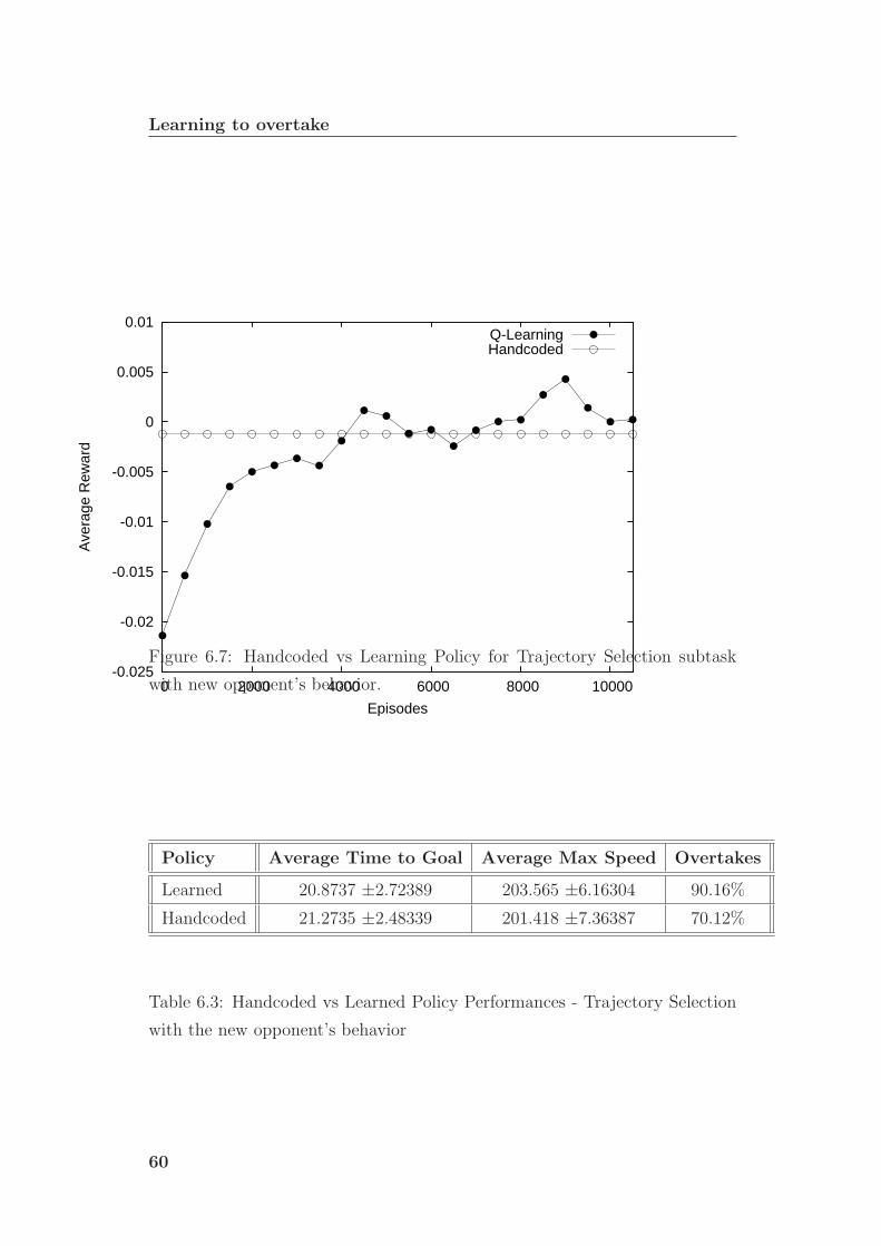
Learning to overtake
-0.025
-0.02
-0.015
-0.01
-0.005
0
0.005
0.01
0 2000 4000 6000 8000 10000
Ave
rage
Rew
ard
Episodes
Q-LearningHandcoded
Figure 6.7: Handcoded vs Learning Policy for Trajectory Selection subtask
with new opponent’s behavior.
Policy Average Time to Goal Average Max Speed Overtakes
Learned 20.8737 ±2.72389 203.565 ±6.16304 90.16%
Handcoded 21.2735 ±2.48339 201.418 ±7.36387 70.12%
Table 6.3: Handcoded vs Learned Policy Performances - Trajectory Selection
with the new opponent’s behavior
60

6.3 Braking Delay
Figure 6.8: Outline of the Braking Delay problem.
6.3.1 Problem definition
Using the normal driving policy we could be found in the situation in which
we are overtaking an opponent but we can’t terminate the surpass because
we need to brake for the incoming turn. In general a good driver in this case
decides to delay the braking action for some time, to complete the overtake.
So we need to learn a new braking policy for this particular situation. What
make this task complicated is the fact that the braking delay must be enough
to terminate the overtake but at the same time not too much, to avoid to
go out of track because of the high speed reached in the turn. Moreover a
driver have also the problem to evaluate the situation to realize if there is the
effective possibility of complete the overtake without go off the track. This
make this task very difficult even for an expert human driver. To successfully
learn a policy for the subtask described above, we must define which are the
relevant data involved in this decision process. We assume that a first necessary
information is the distance of the opponent’s car relative to the one that is
overtaking. Another useful data is the difference of speed from the two cars
and also the distance from the start of the incoming curve. These values are
foundamental to evaluate the dynamics of the overtake and to calculate the
necessary delay to accomplish the surpass avoiding to go off road. Therefore
61

Learning to overtake
the input used as state variables for the learning process are: the opponent’s
frontal distance, defined in the continuous domain [-300, 350], the delta speed,
defined in the continuous domain [-250, 250] and the curve distance, defined
in the continuous domain [0, 1000].
We also define the output of the learning system, defined in the discrete domain
[0, 1]. Such output must be interpreted by the driver as the next action to
perform: if it have a value of 0 the agent don’t modifies the current braking
policy, instead, if the value is 0 the agent modifies the current braking policy,
don’t applying any brake pressure.
In this experiment each learning episode starts when the two cars have reached
a predetermined distance from the next turn and are in an overtake situation.
Note that the episodes don’t always starts exactly in the same conditions of
distances and velocity, because of some casualties in the simulation that can’t
be controlled. The episode ends when the car go off road or when it reaches a
determined point after the curve: in this case the reward is assigned considering
if the car has reached the goal or not. The goal is to have a distance less or
equal to -1 meters with respect of the opponent, that means that the overtake
is successfully accomplished.
Moreover, this is the defined reward function:
rt =
1 if the goal was reached
−1 if the car go off road
0 otherwise
(6.2)
To limit the space of states the domains of all the input variables are
discretized and divided into groups, everyone of which is considered a discrete
state for the corresponding variable. In particular the opponent’s frontal dis-
tance is discretized as { [-300 -15) [-15 -5) [-5 0) [0 1) [1 2) [2 5) [5 10) [10 15)
[15 30) [30 100) [100 350] }, the delta speed as { [-250 0) [0 5) [5 10) [10 20)
[20 50) [50 250] } and the curve distance is discretized as { [0 1) [1 2) [2 5) [5
10) [10 20) [20 50) [50 100) [100 1000] }.The first and last inputs are measured in meters: the opponent’s frontal dis-
tance have a negative value when the driver is located in front of the opponent’s
car and have a positive value if the driver is located behind the opponent. The
information of how much fast the driver is approaching the opponent, repre-
sented by the delta speed variable, is expressed as the difference between the
62
6.3 Braking Delay
speed of the agent’s car and the speed of the opponent’s car (this value is
measured in kilometers per hour). The value of this state variable is negative
when the driver have a lower speed with respect to the opponent.
Finally, the control time chosen for this subtask is of 10 TORCS’s simulation
time steps, corresponding to 0.2 real seconds in the simulated environment.
6.3.2 Experimental results
The parameter setting of the Q-Learning algorithm in this experiment is: α0 =
0.5, γ = 0.95, δα = 0.05, ε0 = 0.5, δε = 0.0005. The algorithm has been stopped
after 12000 episodes.
The car has learned the new subtask with success: the car accomplish the
overtake in nearly all the cases, only rarely remain behind the opponent after
the turn and nearly never go off road.
In Figure 6.9 is reported the value of the average reward for the learning policy
compared with the reference policy, obtained with a mobile average. You can
see that the learned policy exploits an higher value of average reward with
respect of the handcoded one: this is explained by the fact that the learning
system has taken advantage of the new policy, while the handcoded bot, using
the standard braking policy, succeeds to overtake only some times.
In Table 6.4 we compare the performances of the learned, handcoded and
random policy. The measures used for the comparison are the percentage
values of the episodes ended with successfully overtake, with unsuccessfully
overtake and with the car gone off road. The measures are taken from 1000
episodes. As you can see from these results, the learned policy have very dif-
ferent performances with respect to the handocoded one, although the learned
policy adopt a behavior that sometimes may be risky. Moreover from these
results you can notice that a random braking delay policy obtains very bad
performances: this means that it is necessary to learn a reasonable and suitable
policy to accomplish the goal of this subtasks.
63

Learning to overtake
-0.04
-0.02
0
0.02
0.04
0 2000 4000 6000 8000 10000 12000
Ave
rage
Rew
ard
Episodes
Q-LearningHandcoded
Figure 6.9: Handcoded vs Learning Policy for the Braking Delay subtask.
Policy Successes Unsuccesses Off Road
Learned 88.1% 6.7% 5.2%
Handcoded 18.8% 81.2% 0%
Random 0.96% 15.2% 75.2%
Table 6.4: Handcoded vs Learned Policy Performances - Braking Delay
64

6.4 Adapting the Braking Delay to a changing wheel’s friction
6.4 Adapting the Braking Delay to a changing
wheel’s friction
As discussed in Section 3.1.2 the adaptation of the AI in computer games can
offer an improved experience to a game. This dynamic adaptation during the
game can be achieved applying IGL techniques, that mean allowing a pre-
learned policy to continue to learn during a game session to adapt to new
conditions in the environment or to the particular player preferences.
To realize such dynamic policy in our work, we use the Braking Delay subtasks.
We want to use the braking delay policy learned in the previous experiment
in a game session in which we have a change in the environment. We choose
to use the wheel’s friction as the variable environmental condition, simulating
the wheel consumption during a race. What we want to obtain is a policy that
can adapt itself to this change, maintaining a good performance during all the
race.
6.4.1 Problem definition
Using the policy learned in the previous experiment we can successfully com-
plete an overtake approaching a turn. But what happen if the wheel’s friction
decrease during the race? The learned policy could perform badly, because
with less friction we must reach the turn with less speed to avoid to go off
road. So we need to adapt the learned policy during the race, applying the
IGL.
In this experiment the wheel’s friction is progressively decreased from the 100%
to the 85% of the standard value. The friction’s value is setup to decrease by
steps of 3.75%. In particular the value start normally, then is decreased of
one step after 1000 episodes, and then is ulteriorly decreased of one step every
2000 episodes.
The input used as state variables for the learning process are the same of the
previous case: the opponent’s frontal distance, the delta speed and the curve
distance.
We also define the output of the learning system, the reward function and the
control time step as in the previous experiment.
We remember that each learning episode starts when the two cars have reached
65

Learning to overtake
a predetermined distance from the next turn and are in an overtake situation.
The episode ends when the car go off road or when it reaches a determined
point after the curve: in this case the reward is assigned considering if the
car has reached the goal or not. The goal is to have a distance less or equal
to -1 meters with respect of the opponent, that means that the overtake is
successfully accomplished.
6.4.2 Experimental results
The Q-Learning algorithm in this experiment start with the learned policy and
continues to learn with these parameter setting: α0 = 0.4, γ = 0.95, δα = 0.0,
ε0 = 0.01, δε = 0.0. The algorithm has been stopped after 12000 episodes.
In Figure 6.10 is reported the value of the average reward for the learning
policy compared with the reference policy, obtained with a mobile average.
Note that in this case the reference policy isn’t the handcoded one, but the
policy learned in the previous experiment. You can see that the learning
involves only a slight decrease of performance with respect to the reference
policy. In the first three decreasing of the friction the policy maintain an aver-
age reward similar to the one of the reference policy. After the last decreasing
the friction’s change become sufficient to allow the emerging of a new policy,
that the learning process can exploit. Note that the average reward exploited
by the policy in this final situation exceed also the value that it have in the
previous condition. This is explained by the fact that the change of the fric-
tion’s value also affect the opponent’s car. Therefore in the last condition the
learning process can exploit a braking strategy that allows an higher reward.
6.5 Summary
In this Chapter we presented an higher level task, the overtaking strategy and
the experiments that aim to learn a policy for this problem. In the first section
we showed that this task can be further decomposed into two subtasks: the
Trajectory Selection and the Braking Delay, everyone of which corresponds to
a different behavior for overtaking. Then we described in detail the Trajectory
Selection subtask and we showed that it can be solved with Q-Learning. In
addition we showed that our approach can be extended to different environmen-
66

6.5 Summary
0.01
0.015
0.02
0.025
0.03
0.035
0.04
0.045
0.05
0 2000 4000 6000 8000 10000 12000
Ave
rage
Rew
ard
Episodes
Learning DisabledLearning Enabled
Figure 6.10: Learning Disabled vs Learning Enabled Policy for Brake Delay
with decreasing wheel’s friction.
tal conditions, i.e. different versions of the aerodynamic model and different
opponent’s behaviors. Finally we described the second subtask, the Braking
Delay. Firstly we applied the Q-Learning algorithm for learning a good policy
for this subtasks and then we showed that the learned policy can be adapted
to a change in the environment during the learning process.
67

Chapter 7
Conclusions and Future Works
7.1 Conclusions
In this thesis we studied the problem of applying machine learning techniques
to computer games. After presenting the problem in general terms, we dis-
cussed some works related to ML applied to different genres of games. Then
we discussed the reasons why we have chosen the racing car simulators game’s
category as testbed for our work. Among the available open source racing
simulators we’ve chosen The Open Racing Car Simulator (TORCS) for our
thesis.
We’ve discussed the reasons why TORCS was our preferred choice. We pre-
sented a detailed description of TORCS: first of all we analyzed the simulation
engine of the game, explaining how it works and what are its main limitation.
Then we discussed the problem of interfacing TORCS with the PRLT learning
system, that is used in this work to apply the RL methods in the simulation.
We used the RL techniques because they have the advantage that there isn’t
the need to know a priori which are the optimal actions in every state: we
just need to define the reward function and, therefore, we need to know in
advance just which are the negative situations and the goal we want to reach.
Moreover RL is suitable to learn policies that adapts to the user’s preferences
or to changes in the game’s environment.
We presented the context in which is placed this work, and we applied
the principles of the task decomposition to the complex task of driving a car,
presenting a possible decomposition. Then we analyzed the first simple subtask

Conclusions and Future Works
considered, the gear shifting: we’ve seen that is possible to learn this task with
Q-Learning and that this algorithm was capable of exploit a good gear shifting
policy.
We presented an higher level task, the overtaking strategy and the experi-
ments that aim to learn a policy for this problem. Firstly we showed that this
task can be further decomposed into two subtasks: the Trajectory Selection
and the Braking Delay, everyone of which corresponds to a different behavior
for overtaking. Then we described in detail the Trajectory Selection subtask
and we showed that it can be solved with Q-Learning. In addition we showed
that our approach can be extended to different environmental conditions, i.e.
different versions of the aerodynamic model and different opponent’s behav-
iors. Then we described the second subtask, the Braking Delay. Firstly we
applied the Q-Learning algorithm for learning a good policy for this subtasks
and then we showed that the learned policy can be adapted to a change in the
environment during the learning process.
In conclusion with this thesis we’ve shown that it is possible to apply
the method of task decomposition to the complex task of driving a car in a
racing game and consequently to successfully learn some subtasks using the Q-
Learning RL algorithm. We also analyzed the policy learned for the overtaking
strategy at the variation of some game’s conditions, i.e. the aerodynamic cone,
the driving policy of the opponent’s bot and the wheel’s friction. The study
of the learning process at the variation of the aerodynamic model studied
in Chapter 6 shows that the RL approach have the potentiality to allow an
improvement to the development phase of a computer game, supporting the
task division between the developers. In fact is not necessary to exactly know
how the physics engine works to model a bot that have good behaviors: it
is only needed to know which are the goals we want to reach. This is very
important if we consider the modern computer games, that implements more
and more complex physics engine, making difficult to realize good handcoded
policy for the opponents. Finally we’ve analyzed the possibility of using a
learned policy to continue the learning during a game session, to try to adapt
such policy to some environmental changes.
70

7.2 Future Works
7.2 Future Works
This work represents a starting point for the application of ML, and in partic-
ular RL, to computer racing games. From our thesis are emerged interesting
possibilities and therefore it offers several ideas on the possible future devel-
opments, that can be concentrated on different aspects.
Fitted Reinforcement Learning The tasks presented in our decomposi-
tion can be learned using various RL techniques. On the basis of our experience
and as suggested by the experimental results, an interesting possibility is to
pass from an algorithm that uses a tabular representation to another one that
use a function approximation technique. This can be done, for example, by
using the Fitted Reinforcemen Learning [?], a technique in which the algorithm
uses a set of tuples gathered from observation of the system together with the
function computed at the previous step to determine a new training set which
is used by a supervised learning method to compute the next function of the
sequence.
Other Tasks and Integration Another possible future work is to learn
other interesting subtasks from the proposed task decomposition, e.g. the
collision avoidance or the strategy to avoid to be overtaked. Moreover it is
possible to apply ML to integrate different subtasks to obtain an higher level
and more complex behavior.
Adapting Computer Games to the User Finally an interesting future
work can be the using of supervised ML techniques to model the user’s behavior
or preferences: this can make the games more interesting for each single user.
Moreover there is the opportunity to make a deep analysis about the possibility
of applying the IGL method to this kind of problem. In fact there are some
open issue regarding this topic, e.g. the problem of maintaining a certain level
of performace during the IGL and the problem of adapt to the game’s changes
in a reasonable time.
71

Bibliography
[1] The open racing car simultaor website. http://torcs.sourceforge.net/.
[2] Microsoft’s forza motorsport drivatar website, 2005.
http://research.microsoft.com/mlp/forza.
[3] Prlt website, 2007. http://prlt.elet.polimi.it/mediawiki/index.php/Main Page.
[4] D. P. Bertsekas and J. N. Tsitsiklis. Neurodynamic Programming. Athena
Scientific, Belmont, MA, 1996.
[5] B. D. Bryant and R. Miikkulainen. Neuroevolution for adaptive teams.
In In Proceeedings of the 2003 Congress on Evolutionary Computation,
volume 3, pages 2194–2201, 2003.
[6] Louis S. Cole, N. and C. Miles. Using a genetic algorithm to tune first-
person shooter bots. In In Evolutionary Computation, 2004. CEC2004.
Congress on Evolutionary Computation, volume 1, pages 139–145, 2004.
[7] Louis Wehenkel Damien Ernst, Pierre Geurts. Tree-based batch mode
reinforcement learning. 2005.
[8] DARPA. Grand challenge web site, 2005.
http://www.grandchallenge.org/.
[9] D. B. Fogel, editor. Blondie24: Playing at the Edge of AI. 2001.
[10] Hays T. J. Fogel, D. B. and D. R. Johnson. A platform for evolving
characters in competitive games. In In Proceedings of 2004 Congress on
Evolutionary Computation, pages 1420–1426, 2004.

BIBLIOGRAPHY
[11] Hays T. J. Hahn S. L. Fogel, D. B. and J. Quon. A self-learning evo-
lutionary chess program. In Proceeedings of the IEEE, pages 1947–1954,
2004.
[12] J. Furnkranz and M. Kubat, editors. Machine learning in games: A
survey. Nova Science Publishers, 2001.
[13] M. Gallagher and A. Ryan. Learning to play pac-man: an evolutionary,
rule-based approach. In In Evolutionary Computation, 2003. CEC ’03.
The 2003 Congress on Evolutionary Computation, volume 4, pages 2462–
2469, 2003.
[14] M. Gardner. How to build a game-learning machine and then teach it to
play and to win. Scientific American, (206):138–144, 1962.
[15] B. Geisler. An Empirical Study of Machine Learning Algorithms Ap-
plied to Modeling Player Behavior in a First Person Shooter Video Game.
PhD thesis, Department of Computer Sciences, University of Wisconsin-
Madison, Madison, WI, 2002.
[16] Jeff Hannan. Interview to jeff hannan, 2001.
http://www.generation5.org/content/2001/hannan.asp.
[17] J.-H. Hong and S.-B. Cho. Evolution of emergent behaviors for shooting
game characters in robocode. In In Evolutionary Computation, 2004.
CEC2004. Congress on Evolutionary Computation, volume 1, pages 634–
638, 2004.
[18] T. Jaakkola, M. Jordan, and S. Singh. On the convergence of stochas-
tic iterative dynamic programming algorithms. Neural Computation,
6(6):1185–1201, 1994.
[19] Leslie Pack Kaelbling, Michael L. Littman, and Andrew W. Moore. Re-
inforcement Learning: A Survey. Journal of Artificial Intelligence Re-
search, 4, 1996. HTML version: http://www.cs.brown.edu/people/lpk/rl-
survey/rl-survey.html.
[20] Bobby D. Bryant Kenneth O. Stanley and Risto Miikku-
lainen. Real-time neuroevolution in the nero video game. 2005.
http://nn.cs.utexas.edu/downloads/papers/stanley.ieeetec05.pdf.
74

BIBLIOGRAPHY
[21] Adele E. Howe Larry D. Pyeatt and Charles W. Anderson. Learning
coordinated behaviors for control of a simulated race car. 1995.
[22] D. Michie. Trail and error. Penguin Science Survey, (2):129–145, 1961.
[23] I. Parmee and C. Bonham. Towards the support of innovative concep-
tual design through interactive designer/evolutionary computing strate-
gies. Artificial Intelligence for Engineering Design, Analysis and Manu-
facturing Journal, (14):3–16, 1999.
[24] J. Peng and R. J. Williams. Efficient learning and planning within the
Dyna framework. Adaptive Behaviour, 2:437–454, 1993.
[25] J. Peng and R. J. Williams. Incremental multi-step Q-learning. Machine
Learning, 22:283–290, 1996.
[26] Larry D. Pyeatt and Adele E. Howe. Learning to race: Experiment with
a simulated race car.
[27] T. Revello and R. McCartney. Generating war game strategies using
a genetic algorithm. In In Evolutionary Computation, 2002. CEC ’02.
Proceedings of the 2002 Congress on Evolutionary Computation, volume 2,
pages 1086–1091, 2002.
[28] Craig Reynolds. Game research and technology website.
http://www.red3d.com/cwr/games/.
[29] Moriarty D. McQuesten P. Richards, N. and R. Miikkulainen. Evolving
neural networks to play go. In In Proceedings of the Seventh International
Conference on Genetic Algorithms, 1997.
[30] G. A. Rummery and M. Niranjan. On-line Q-learning using connection-
ist systems. Technical Report CUED/F-INFENG/TR 166, Cambridge
University Engineering Department, September 1994.
[31] A. L. Samuel. Some studies in machine learning using the game of check-
ers. IBM Journal, (3):210–229, 1959.
[32] Risto Miikkulainen Shimon Whiteson, Nate Kohl and Peter Stone. Evolv-
ing soccer keepaway players through task decomposition. 2005.
75
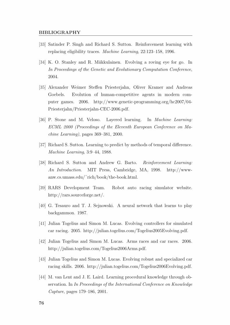
BIBLIOGRAPHY
[33] Satinder P. Singh and Richard S. Sutton. Reinforcement learning with
replacing eligibility traces. Machine Learning, 22:123–158, 1996.
[34] K. O. Stanley and R. Miikkulainen. Evolving a roving eye for go. In
In Proceedings of the Genetic and Evolutionary Computation Conference,
2004.
[35] Alexander Weimer Steffen Priesterjahn, Oliver Kramer and Andreas
Goebels. Evolution of human-competitive agents in modern com-
puter games. 2006. http://www.genetic-programming.org/hc2007/04-
Priesterjahn/Priesterjahn-CEC-2006.pdf.
[36] P. Stone and M. Veloso. Layered learning. In Machine Learning:
ECML 2000 (Proceedings of the Eleventh European Conference on Ma-
chine Learning), pages 369–381, 2000.
[37] Richard S. Sutton. Learning to predict by methods of temporal difference.
Machine Learning, 3:9–44, 1988.
[38] Richard S. Sutton and Andrew G. Barto. Reinforcement Learning:
An Introduction. MIT Press, Cambridge, MA, 1998. http://www-
anw.cs.umass.edu/˜rich/book/the-book.html.
[39] RARS Development Team. Robot auto racing simulator website.
http://rars.sourceforge.net/.
[40] G. Tesauro and T. J. Sejnowski. A neural network that learns to play
backgammon. 1987.
[41] Julian Togelius and Simon M. Lucas. Evolving controllers for simulated
car racing. 2005. http://julian.togelius.com/Togelius2005Evolving.pdf.
[42] Julian Togelius and Simon M. Lucas. Arms races and car races. 2006.
http://julian.togelius.com/Togelius2006Arms.pdf.
[43] Julian Togelius and Simon M. Lucas. Evolving robust and specialized car
racing skills. 2006. http://julian.togelius.com/Togelius2006Evolving.pdf.
[44] M. van Lent and J. E. Laird. Learning procedural knowledge through ob-
servation. In In Proceedings of the International Conference on Knowledge
Capture, pages 179–186, 2001.
76

BIBLIOGRAPHY
[45] Zhijin Wang and Chen Yang. Car simulation using reinforcement learning.
[46] C.J.C.H. Watkins. Learning from Delayed Rewards. PhD thesis, King’s
College, Cambridge, UK, May 1989.
[47] C.J.C.H. Watkins and P. Dayan. Technical note: Q-Learning. Machine
Learning, 8:279–292, 1992.
[48] Stewart W. Wilson. Explore/exploit strategies in autonomy. pages 325–
332.
[49] Bernhard Wymann. TORCS Robot Tutorial, 2005.
http://www.berniw.org/.
[50] Levine J. Yannakakis, G. and J. Hallam. An evolutionary approach
for interactive computer games. In In Evolutionary Computation, 2004.
CEC2004. Congress on Evolutionary Computation, volume 1, pages 986–
993, 2004.
[51] Ishii S. Yoshioka, T. and M. Ito. Strategy acquisition for the game othello
based on reinforcement learning. In S. Usui and T. Omori, editors, In
Proceedings of the Fifth International Conference on Neural Information
Processing, pages 841–844. Morgan Kaufmann, 1998.
77


![Version Control with Git - Politecnico di Milanohome.deib.polimi.it/...media=teaching:aos:2017:aos_l2_version_control_with_git.pdf · [--git-dir=] [--work-tree=]](https://static.fdocuments.in/doc/165x107/5dd098dcd6be591ccb61c348/version-control-with-git-politecnico-di-teachingaos2017aosl2versioncontrolwithgitpdf.jpg)