15 February 2019

POLITECNICO DI TORINORepository ISTITUZIONALE

Case study: A GPR survey on a morainic lake in northern Italy for bathymetry, water volume and sedimentcharacterization / Sambuelli L.; Bava S.. - In: JOURNAL OF APPLIED GEOPHYSICS. - ISSN 0926-9851. -ELETTRONICO. - 81(2012), pp. 48-56.

Original

Case study: A GPR survey on a morainic lake in northern Italy for bathymetry, water volume andsediment characterization

Publisher:

PublishedDOI:10.1016/j.jappgeo.2011.09.016

Terms of use:openAccess

Publisher copyright

(Article begins on next page)

This article is made available under terms and conditions as specified in the corresponding bibliographic description inthe repository

Availability:This version is available at: 11583/2495492 since:

Elsevier

This document is the post-print (i.e. final draft post-refereeing) version of an article published in the journal Journal of Applied Geophysics. Beyond the journal formatting, please note that there could be minor changes and edits from this document to the final published version. The final published version of this article is accessible from here: http://dx.doi.org/10.1016/j.jappgeo.2011.09.016. This document is made accessible through PORTO, the Open Access Repository of Politecnico di Torino (http://porto.polito.it), in compliance with the Publisher’s copyright policy as reported in the SHERPA-ROMEO website: http://www.sherpa.ac.uk/romeo/search.php?issn=0926-9851 Preferred citation: this document may be cited directly referring to the above mentioned final published version: Bava S., Sambuelli L. Journal of Applied Geophysics. Case study: A GPR survey on a morainic lake in northern Italy for bathymetry, water volume and sediment characterization (2012), 81, pp 48-56.  

Pagina 1 di 21

Title: APPGEO1855 Case study: A GPR survey on a morainic lake in northern Italy for bathymetry, water volume and sediment characterization. Authors: Luigi Sambuelli, Silvia Bava. Affiliation: Politecnico di Torino Dipartimento di Ingegneria del Territorio, dell’Ambiente e delle Geotecnologie Address: C.so Duca degli Abruzzi, 24 - 10129 – Torino – Italy Reference Author: Luigi Sambuelli e-mail: luigi.sambuelli@polito.it Keywords: GPR; Sediment porosity, Lacustrine Abstract We carried out an extensive waterborne GPR survey consisting of 50 profiles with a total length of

nearly 37 km on the morainic lake of Candia northerly Turin (Italy). Our aim was to test the

capability of GPR to estimate the bathymetry, the water volume and the sediment type. We

enhanced and controlled the GPR data processing and interpretation with bathymetry acquired with

an acoustic echo sounder and measured conductivity and temperature profile of the water column

with a multiparametric probe. We also analysed the diffraction hyperbola that originated within the

sediments in order to estimate the velocity and relative permittivity. With the permittivity and

dielectric mixing rules, we estimated the porosity of the sediments above the diffracting objects and

drew a map of the bottom lake porosity.

Pagina 2 di 21

1. Introduction

Here we discuss an extensive waterborne GPR survey of a morainic lake in northern Italy that we

performed along with an echo-sounder and spotted measurements along the water column with a

multiparametric sonde. The survey aimed to evaluate the capability of a non-seismic tool as the

GPR to estimate the water volume and the bottom sediment type.

The use of non-seismic methods to investigate sediments beneath shallow freshwater has

increased in the last twenty years (Sambuelli and Butler, 2009; Butler, 2009). Monitoring river

erosion, lake filling and understanding the connection between surface water and underground

water are critical environmental issues. Many publications related to the application of GPR to

shallow-water environments can be found in literature. Annan and Davis (1977) and Kovacs (1978)

conducted some early applications of GPR in low-conductivity melting water in arctic areas. In

such low-conductivity environments a noticeable subbottom penetration in water depths exceeding

25 m can be achieved (Delaney et al., 1992). Bathymetric maps and sediments morphology of ice-

covered lakes (Moorman and Michel, 1997; Schwamborn et al., 2002) rivers and reservoirs (Arcone

et al., 1992; Best et al., 2005; Hunter et al., 2003) have been reported as well. In temperate areas

GPR has been tested for monitoring stream discharge (Haeni et al., 2000; Melcher et al., 2002;

Cheng et al., 2004; Costa et al., 2006), studying bottom deposits (Arcone et al., 2006; Buynevich

and Fitzgerald, 2003; Fuchs et al., 2004; Shields et al., 2004; Moorman et al., 2001, Sambuelli et

al., 2009), mapping bathymetry (Powers et al., 1999) and subbottom strata (Arcone et al., 2010).

GPR could provide complementary information to seismic methods, especially in very shallow

water where reverberation can prevent the interpretation of subbottom reflectors or when gas

pockets in sediments rich in organic matter block seismic signal penetration (Delaney et al., 1992;

Schwamborn et al., 2002; Arcone et al., 2006; Mellet, 1995). Waterborne GPR can be used in many

different setups: case histories report the use of antennas directly coupled to water from the surface

(Mellet, 1995; Sellmann et al., 1992), noncontact systems such as helicopter mounts (Melcher et al.,

2002) or hanging slings (Haeni et al., 2000; Cheng et al., 2004; Costa et al., 2000), and antennas

mounted on the bottom of non-metallic boats (Sambuelli et al., 2009; Sellmann et al., 1992,

Bradford et al., 2005; Jol and Albrecht, 2004; Porsani et al., 2004; Park et al., 2004). The potential

of GPR to allow estimates bottom sediment types has been mentioned by Ulriksen (1982), who

suggested that fine sediments can be identified from smooth reflectors, rough surfaces such as

moraine can be identified from speckled and weak signals, while boulders may produce hyperbolic

diffractions. As a rule of thumb the coarser is the sediment then the higher are the amplitudes of the

reflected GPR signals. The same qualitative approach to the analysis of basin-bottom characteristics

has been tested positively by other authors (Mellet, 1995, Beres and Haeni, 1991). In particular,

Pagina 3 di 21

Dudley and Giffen (1999) found optimal agreement between GPR results and direct sampling of

sediments. Recently some more quantitative approaches to the discrimination of sediment type

using the amplitude of the GPR signal reflected from the water bottom have been proposed

(Sambuelli et al., 2009; Lin et al., 2010).

Estimating the bathymetry and discriminating sediment types by analysing the time delay and

amplitude of reflections mainly assumes that the water is homogeneous. This assumption is valid in

shallow rivers or lakes where there is little or no thermocline and therefore no reflectors before the

bottom, but must be questioned for deeper lakes (Bradford et al., 2007).

2. Site description

The lake of Candia (Turin, Italy) is an example of inter-moraine lake belonging to the morainic

amphitheatre of Ivrea, northerly the town of Turin (Figure 1). The lake (226 m a.s.l.) has a surface

of about 1.52 km2, a perimeter of about 5.5 km and an estimated volume of about 7.2 Mm3. The

amphitheatre was built up by the Balteo Glacier which flowed through the Aosta Valley during the

Quaternary period. The Balteo Glacier had an average width of 3 km, a thickness of around 600 m

and was spread over 300 km through the Alps. At its maximum expansion it went down to 25 km

into the Po plain with a width of about 20 km, reaching today’s northern border of the town of

Turin. According to recent studies the lake of Candia was left after the recession of the Riss

Glaciation (about 150000 years ago). The lake of Candia then settled in a plain that was eroded by

the advancing glacier and then refilled to a far lower extent by the glacial deposits of the glacier

retreat. According to Gianotti et al. (2008), the Candia lake lies on the Piverone alloformation (Late

Pleistocene) above the Serra alloformation (end of the Middle Pleistocene) each one referable to a

different glacial episode.

A borehole (Alice Superiore borehole) drilled about 20 km NNW in the same geological

environment gave the stratigraphic log reported in Figure 2. It is evident the dominance of more or

less dense gravels with boulders that may be included in the mud. A palustrine gyttja layer made by

peaty brown clay represents the interstadial episode between the two glacial events. Until about 50

years ago, before an eutrophication process took place, it was possible to see the white gravels of

the lake bottom and the fresh water columns rising up to the surface of the lake from underwater

springs. Today, the silts and the vegetation prevent the view of the lake bottom. The lake has

neither affluent nor effluent but a small ditch used sometimes for irrigation; the water recharge is

from rains and underwater springs.

3. Methods

Pagina 4 di 21

3.1 Data acquisition

We acquired the GPR data with a K2 Ids radar and a Subecho-70 monostatic antenna with peak

frequency in air at 89 MHz. We placed the antenna at the bottom of a fiber-reinforced plastic boat

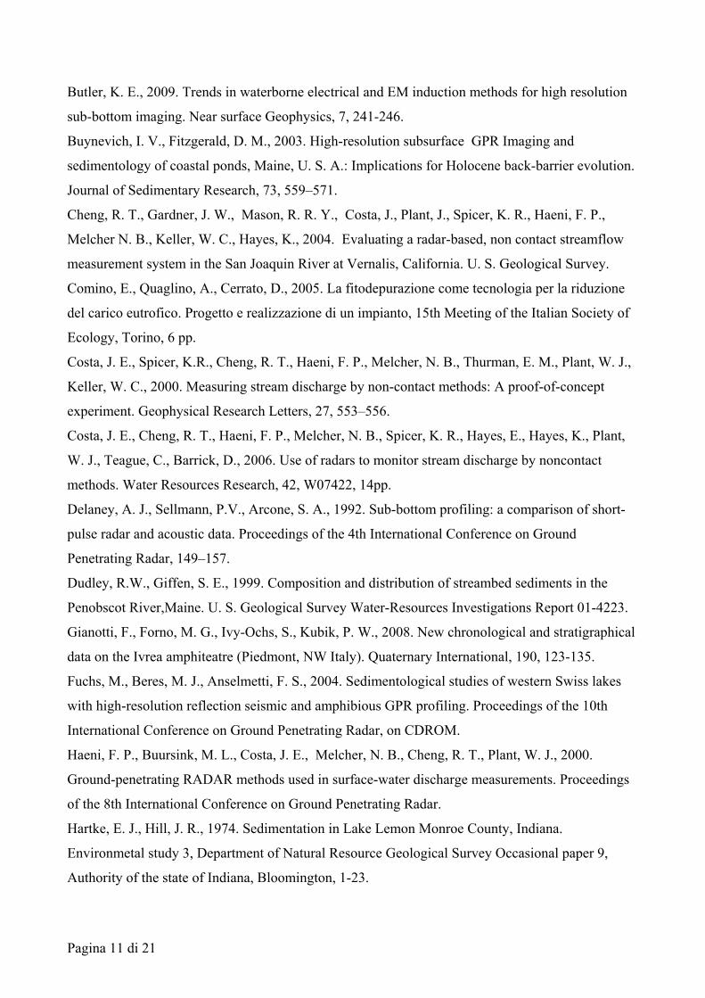
and the routes of the profiles were planned and tracked with a Garmin GPS60. We acquired 50 GPR

profiles for a total length of about 37 km (Figure 3) at a sampling frequency of 1.7 GHz, trace

length of 600 ns and a traces interval of 4 cm. Neither filters nor gains were used during the

acquisition.

We also acquired bathymetry with a 170kHz Airmar DT800 echo sounder. The dominant

wavelength in water roughly equalled 1 cm, and our average sampling interval was 1 m. The echo

sounder probe was fixed at the side of the boat and approximately aligned with the centre of the

GPR antenna. We also used a Hydrolab Datasonde 4 Multi-Parametric Probe (MPP) to measure

temperature, T, and conductivity, σ , along the water column at three points on the lake (Figure 3).

3.2 Data processing

We needed to estimate the water conductivity to evaluate the GPR signal attenuation and the water

permittivity to evaluate the GPR pulse velocity. We also estimated the dominant frequency of the

GPR pulse by doing a spectral analysis of windowed reflected pulses from different water depths.

The results shown a dominant frequency range from 66 to 80 MHz with a mode around 70 MHz

which was the value selected for further calculations. As a solution to Maxwell’s equations the

amplitude at a distance z and time t of the electric field E(z, t,ω) associated with a monochromatic

plane wave of angular frequency ω is

( ) ( ) ( )0 0, , , , i t kzE z t E z t e ωω ω += , 1

where E(z0,t0,ω) is the amplitude at reference time and distance t0 and z0. The quantity

w ww

k ivωα= + 2

is the complex wave number (subscript w refers to water) where

2

00

0

1 12

w ww w

w

ε ε σα ω μ μ

ε ε ω

⎛ ⎞⎛ ⎞⎜ ⎟= + −⎜ ⎟⎜ ⎟⎝ ⎠⎝ ⎠

3

and

2

00

0

1

1 12

w

w ww

w

vε ε σ

μ με ε ω

=⎛ ⎞⎛ ⎞⎜ ⎟+ +⎜ ⎟⎜ ⎟⎝ ⎠⎝ ⎠

4

Pagina 5 di 21

are respectively, the attenuation factor due to dissipative phenomena and the phase velocity . Given

μ0=4π×10-7 [H/m], µw=μ0, ε0=(36π)-1×10-9 [F/m] and ω=2π×70×106 [rad/s], we need εw and σw to

evaluate αw and vw.

The MPP gives the T and σw so that we calculated the permittivity using the formula given by

Nyshadam et al. (1992):

009.01000141.01009398.0100008.474.87 33221 ±×−×−×−= −−− TTTwε 5

The average salinity of the lake water was about 0.06 ppt (part per thousand) and so the correction

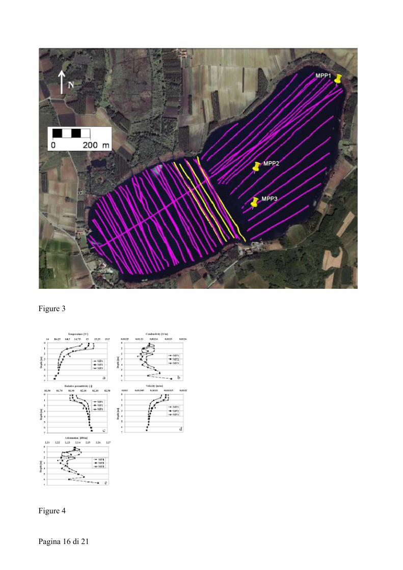
to apply to eq. 5 for such values of salinity is negligible. We plotted the T and the σw along the

water columns according to the MPP data (Figure 4 a,b). The small temperature gradient below the

first meter was so small and showed such small variations (Figure 4 c,d,e) that we rejected the

hypothesis of a thermo cline. We then used the following values of velocity and attenuation in the

GPR processing: vw=0.033 [m/ns] and αw=2.24 [dB/m].

We processed the GPR profiles with the Reflexw® software. We corrected for the direct arrival

delay and eliminated the very low frequency trend. We band-pass filtered from 20 to 190 MHz with

a Butterworth filter to attenuate both low and high frequency noise and then resampled the traces to

obtain a trace interval of 0.2 m. We removed the steady background horizontal continuous signals

with a spatial high-pass filter. We applied firstly a divergence compensation, using vw, to recover

the amplitude attenuation due to the geometrical spreading, and then secondly an exponential gain,

using αw, to recover the amplitude decrease due to the dissipation related to the water conductivity.

As far as the wavelength is concerned, the dominant wavelength of the GPR signal bottom

reflection ranged from about 0.4 m in the more shallow waters to about 0.5 m in the deepest. To

enhance the continuity of the reflectors we then applied a horizontal running average over 11 traces

that, giving the new spatial sampling interval, roughly corresponds to a low pass filter that

attenuates the wavelengths shorter than 2 m. We then picked the first break of the first bottom

reflection to estimate the bathymetry of the lake and to calculate the volume of water. Finally we

applied a muting above the picked times to cancel out residual noise in water. In the following some

processed radragrams will be presented.

To assess the bathymetry given by the GPR we compared the water depths to those obtained

with the acoustic sounder. On average the difference between the two bathymetric data was about

0.17 m with a standard deviation of 0.14 m. This discrepancy could be caused by different

reflecting boundaries because the acoustic signal should have no penetration whereas the GPR

signal is sensitive to subtle near surface layering. This difference could also be enhanced by the

Pagina 6 di 21

largely different wavelengths so that the leading edges of the pulses could be differently estimated.

It could be also due to the fact that the echo sounder sensor was roughly connected to the boat side

and we could not account for the exact depth of the sensor below the water surface nor its rolling

and pitching with respect to the boat.

To estimate the bottom sediment porosity we used the diffraction events that later than the

bottom lake reflection. The diffractions are caused by point-like objects within the sediments. The t

and x coordinates of these events obey the following equations

( ) ( )1 2

1 2

2 2cos cos

h htv i v r

= + 6

and

( ) ( )1 2tan tanx h i h r= + , 7

where h1 is the water depth above the vertex of the diffraction pattern, h2 is the thickness of

sediment above the vertex, i is the incident angle, r is the refracted angle and v1 and v2 are,

respectively, the velocity of GPR wave in water and in sediment (Figure 5). The incident and the

refracted angles i and r, v1 and v2 are related by Snell’ s law

( )( )

1

2

sinsin

i vr v

= 8

For each one of the diffraction events within the radargrams we can read n experimental data

pairs (te, xe), 2h1/v1 and 2h2/v2. These latter are respectively, the two-way-traveltime (twt) of the

reflection from water-sediment interface above the event vertex (i.e., t1) and the twt relative to the

path within the sediments from the above mentioned point to the vertex of the event (i.e., t2).

However, the two equations [6, 7] cannot be solved for a unique solution in the form t=t(x).

Therefore we set up a procedure to determine the unknowns h2 and v2 which consists of fitting the

(te, xe) with (t, x) obtained from equations [6, 7] by spanning all possible incident angles with values

of v2 ranging from the velocity in water to the velocity in air. We then found the sediment velocity

v2 by searching for the minimum of a misfit function between calculated and experimental

traveltimes related to each diffraction event. To have a more robust estimate, less sensitive to

outliers, the selected function was the mean absolute difference (mad) that is:

Pagina 7 di 21

et tmad

N−

= ∑ , 9

where te are the experimental picked twt in xe, t are the calculated twt in xe and N is the number of

twt’s considered for each diffraction event. A simplified script referring to the routine implemented

for the procedure is reported in Appendix A.

We assessed the effectiveness of this procedure by performing a synthetic test with the finite

difference modeller contained in the Reflexw® software. We built a model consisting of a point-

like scattering target within sediments under a water layer . The synthetic GPR pulse had a

dominant frequency of 100 MHz; the scatter source had a diameter D = 0.16 m and the dominant

wavelength of the GPR signal was λ=0.32 m. In Figure 5 a sketch of the geometry implied in

equations 6, 7, 8 with the main physical and geometrical parameters used for the synthetic model is

shown. In Figure 6a, b the model and the synthetic radargram are respectively shown. The fitting

procedure results were ε2=25.06 and h2=1.72 m, with a relative percent error with respect to the

expected values respectively of 0.24% and 1.16%.

We then selected the clearest diffraction events along the profiles and, according to the proposed

procedure, estimated the local porosities. In Figures 7 and 8a, 8b an example of the aforementioned

procedure is shown. Figure 7 shows one of the selected diffraction events observed beneath the

bottom sediment. Figure 8a shows the trend of the misfit function between calculated and observed

data. Figure 8b shows the fitting between experimental and calculated (twt, x) pairs. Over the 51

diffraction events we analysed we had the following statistical figures: mean(min(mad)) = 0.95 ns,

st.dev.(min(mad)) = 1.16 ns. We considered these statistical results positively. In fact the sampling

interval during acquisition was 0.588 ns so that the mean of the selected mad’s (mean(min(mad)))

was less than twice the sampling interval of the radar traces.

We then inserted the v2 values, converted in the dielectric permittivity of sediments εs, in a

mixing rule that, given the dielectric permittivity of water and solid particles, allowed the local

sediment porosity (Sambuelli, 2009) to be estimated. Among the many mixing formulas available

we selected the Maxwell (Equation 10) (Maxwell, 1892) and the so called CRIM (Birchak et al.,

1974) which are

( )( )3

2s ss

ww w s

ε εφ ε

ε ε ε ε−

=+ −

, 10

and

s ss

w ss

ε εφ

ε ε−

=−

11

Pagina 8 di 21

respectively, where φ is the porosity, εs the relative permittivity of the sediments calculated from v2,

εw=82 (the relative permittivity of the water taken from the MPP data), and εss=6 is an average

relative permittivity of the solid grains taken from the literature (Reynolds, 1997; Parkhomenko,

1967). We then averaged the porosities.

4. Results and discussion

The GPR survey shows that the bottom of Candia lake consists of two main types of sediment. One

is gravel and pebbles, which shows a high reflectivity and therefore is not penetrated by GPR signal.

The other is organic-rich silt, with a lower reflectivity, more transparent, and allows the underlying

bedding to be detected. In Figure 9 we show the radargrams recorded along the red lines in Figure 3.

From the top to the bottom of the figure the profiles are from East to West. The gravels are clearly

visible as is their progressive cover by the silts going westward. The top radargram, in particular,

shows the high reflectivity of the gravels underlain by a multiple reflection. On the other hand the

transparency of the silt is clearly depicted by the evident reflection of the gravels beneath the silt.

The gravels are likely moraine while the silt (younger) is likely later sedimentation always

superimposed on the gravels. We confirmed the outcropping of the gravels and pebbles of the

moraine by sampling with a Van Veen grab bucket (Figure 10a). We actually found respectively

organic rich slime (Figure 10b) and pebbles (Figure 10c) where the radargrams showed weak and

strong reflections.

By converting the twt’s of the bottom reflections in water depth and using the velocity of the GPR

pulse in water obtained with the MPP, we plotted the bathymetry of the lake (Figure 11). The water

volume we calculated agreed with the value (about 7 Mm3) referred to in literature (Comino et al.,

2005).

In Figure 12 we show a porosity map of the lake bottom (Figure 12). We mapped porosity 0.15

up 0.65. The lowest values are compatible with poorly sorted gravel with sand and silt filling the

spaces between the largest grains. The highest value are compatible with silt or fine sand rich in

organic material. These unusually high porosity values have also been found in the sea bottom

(Ullman and Aller, 1982), and in pond (Avnimelech et al., 2001) and lake bottoms (Hartke and Hill,

1974). Even if the sampled points were few and oddly distributed it seems evident that significant

areas of the bottom sediments have porosity larger than 0.55. These areas have a great role in the

biological and hydro-geochemical processes developing within the lake.

5. Conclusion

Pagina 9 di 21

Our three main results are: the identification of an area of the lake bottom made by the coarse

materials of the moraine, the bathymetry and water volume and the estimated porosity of the bottom

sediments.

The waterborne GPR can be effective to estimate bathymetry of shallow freshwater basins,

together with the bedding and porosity of the bottom sediments, provided that the water resistivity,

using a GPR central frequency ranging from 50 to 100 MHz, is higher than 40 Ωm to reach 3 to 10

m depths. The depth can be even greater if very low conductivity water derives from ice melting.

Profiling of the subbottom bedding largely depends on the bottom sediment type. The finer are the

bottom sediments the lower is their reflectivity the higher is the probability to image strata beneath

the bottom surface. An estimation of the bottom sediment porosity can also be achieved if point-

like scattering targets within the sediments are found. Then our diffraction matching procedure

allows an estimation of the GPR pulse velocity in the sediment and hence, with suitable mixing

rules, a porosity range for the sediment above the scatterers can be derived.

Appendix A

We present a scheme of the script we wrote to implement the procedure for the determination of the

velocity of sediments v2. The knowns quantities are : t1, v1, h1, t2(=h2/2v2), {te}, {xe}. In the script:

vw = velocity in water; vair= velocity in air; te = experimental times picked on the diffraction

hyperbola; xe = coordinate related to te; r = refraction angle; v2 = velocity in sediments. The line

“spline (t, x)→t(x | v2)” means that a cubic spline is used to interpolate the calculated (t ,x) and

calculate the value of t corresponding to each xe coordinate.

for v2 = vw to vair [200 steps] calculate h2 for r = 0° to 75° [25 steps] calculate i (Eq.8) calculate t (Eq.6)

calculate x (Eq.7) next r

spline (t, x)→t(x | v2) calculate t(xe | v2) % calculate the t’s after spline interpolation

read (te) at xe % read the experimental data calculate mad (Eq.9) % using t(xe | v2) and te

next v2 plot (v2, mad) (Figure 8a) % plot mad versus velocity find v*

2 = v2(min(mad)) % find the velocity corresponding to the minimum mad plot t(x | v*

2) and {xe, te}(Figure 8b) % plot the calculated hyperbola and the experimental data

Acknowledgments

Pagina 10 di 21

The Authors would like to thank the “Ente Parco naturale di interesse provinciale del Lago di

Candia” for the permission of working on the lake and publishing the results. Thanks are also due to

Alessandro Arato, Mariantonia Zappone, Corrado Calzoni, Stefano Stocco and Diego Franco for

their help in collecting and processing data. This study has been founded by MIUR GRANT

2007ET8X4C_002: “GeoElectromagnetic Methods for MApping River Sediments (GEMMARS)”

within the project “Groundwater control , protection and management. The contribution of

innovative geophysical methods”. Finally the Authors wish to thank the reviewers whose

suggestions improved the paper.

References

Annan, A. P., Davis, J. L., 1977. Impulse radar applied to ice thickness measurements and

freshwater bathymetry: Report of Activities Part B, Geological Survey of Canada.

Arcone, S. A., Chacho, E. F. J., Delaney, A. J., 1992. Short-pulse radar detection of groundwater in

the Sagavanirktok River floodplain in early spring. Water Resources Research, 28, 2925–2936.

Arcone, S. A., Finnegan, D., Laatsch, J. E., 2006. Bathymetric and subbottom surveying in shallow

and conductive water. Proceedings of the 11th International Conference on Ground Penetrating

Radar, on CDROM.

Arcone, S. A., Finnegan, D., Boitnott, G., 2010. GPR characterization of a lacustrine UXO site.

Geophysics, 75, WA221-WA239.

Avnimelech, Y., Ritvo, G., Meijer, L. E., Kochba, M., 2001. Water content, organic carbon and dry

bulk density in flooded sediments. Aquacultural Engineering, 25, 25-33.

Beres, M., Haeni, F. P., 1991. Application of ground-penetrating-radar methods in hydrogeologic

studies. GroundWater, 29, 375–386.

Best, H., McNamara, J. P., Liberty, L., 2005. Association of ice and river channel morphology

determined using ground-penetrating radar in the Kuparuk River, Alaska. Arctic, Antarctic, and

Alpine Research, 37, 157–162.

Birchak, J. R., Gardner, C. G., Hipp, J. E, Victor, J. M., 1974. High dielectric microwave probes for

sensing soil moisture. Proceedings of the IEEE, 62, 93-98.

Bradford, J. H., McNamara, J. P., Bowden, W., Gooseff, M.N., 2005. Measuring thaw depth

beneath peat-lined arctic streams using ground-penetrating radar. Hydrological Processes, 19,

2689–2699.

Bradford, J. H., Johnson, C. R., Brosten, T., McNamara, J. P., Gooseff, M. N., 2007. Imaging

thermal stratigraphy in freshwater lakes using georadar. Geophysical Research Letters, 34, 1-5.

Pagina 11 di 21

Butler, K. E., 2009. Trends in waterborne electrical and EM induction methods for high resolution

sub-bottom imaging. Near surface Geophysics, 7, 241-246.

Buynevich, I. V., Fitzgerald, D. M., 2003. High-resolution subsurface GPR Imaging and

sedimentology of coastal ponds, Maine, U. S. A.: Implications for Holocene back-barrier evolution.

Journal of Sedimentary Research, 73, 559–571.

Cheng, R. T., Gardner, J. W., Mason, R. R. Y., Costa, J., Plant, J., Spicer, K. R., Haeni, F. P.,

Melcher N. B., Keller, W. C., Hayes, K., 2004. Evaluating a radar-based, non contact streamflow

measurement system in the San Joaquin River at Vernalis, California. U. S. Geological Survey.

Comino, E., Quaglino, A., Cerrato, D., 2005. La fitodepurazione come tecnologia per la riduzione

del carico eutrofico. Progetto e realizzazione di un impianto, 15th Meeting of the Italian Society of

Ecology, Torino, 6 pp.

Costa, J. E., Spicer, K.R., Cheng, R. T., Haeni, F. P., Melcher, N. B., Thurman, E. M., Plant, W. J.,

Keller, W. C., 2000. Measuring stream discharge by non-contact methods: A proof-of-concept

experiment. Geophysical Research Letters, 27, 553–556.

Costa, J. E., Cheng, R. T., Haeni, F. P., Melcher, N. B., Spicer, K. R., Hayes, E., Hayes, K., Plant,

W. J., Teague, C., Barrick, D., 2006. Use of radars to monitor stream discharge by noncontact

methods. Water Resources Research, 42, W07422, 14pp.

Delaney, A. J., Sellmann, P.V., Arcone, S. A., 1992. Sub-bottom profiling: a comparison of short-

pulse radar and acoustic data. Proceedings of the 4th International Conference on Ground

Penetrating Radar, 149–157.

Dudley, R.W., Giffen, S. E., 1999. Composition and distribution of streambed sediments in the

Penobscot River,Maine. U. S. Geological Survey Water-Resources Investigations Report 01-4223.

Gianotti, F., Forno, M. G., Ivy-Ochs, S., Kubik, P. W., 2008. New chronological and stratigraphical

data on the Ivrea amphiteatre (Piedmont, NW Italy). Quaternary International, 190, 123-135.

Fuchs, M., Beres, M. J., Anselmetti, F. S., 2004. Sedimentological studies of western Swiss lakes

with high-resolution reflection seismic and amphibious GPR profiling. Proceedings of the 10th

International Conference on Ground Penetrating Radar, on CDROM.

Haeni, F. P., Buursink, M. L., Costa, J. E., Melcher, N. B., Cheng, R. T., Plant, W. J., 2000.

Ground-penetrating RADAR methods used in surface-water discharge measurements. Proceedings

of the 8th International Conference on Ground Penetrating Radar.

Hartke, E. J., Hill, J. R., 1974. Sedimentation in Lake Lemon Monroe County, Indiana.

Environmetal study 3, Department of Natural Resource Geological Survey Occasional paper 9,

Authority of the state of Indiana, Bloomington, 1-23.

Pagina 12 di 21

Hunter, L. E., Ferrick, M. G., Collins, C. M., 2003. Monitoring sediment infilling at the Ship Creek

Reservoir, Fort Richardson, Alaska, using GPR, in: Bristow, C. S., Jol, H. M., (Eds.), Ground

penetrating radar in sediments: Geological Society of London Special Publication 211, 199–206.

Jol, H. M., Albrecht, A., 2004. Searching for submerged lumber with ground penetrating radar: Rib

Lake. Proceedings of the 10th International Conference on Ground Penetrating Radar, on CDROM.

Kovacs, A., 1978. Remote detection of water under ice-covered lakes on the North Slope of Alaska.

Arctic, 31, 448–458.

Lin, Y. T., Wu, C. H., Fratta, D., Kung, K. J. S., 2010. An integrated acoustic and electromagnetic

wave-based technique to estimate subbottom sediments properties in a freshwater environment.

Near surface geophysics, 8, 213-221.

Maxwell, J.C., 1892. A treatise on electricity and magnetism, Clarendon Press, Oxford, vol.1.

Melcher, N. B., Costa, J. E., Haeni, F. P., Cheng, R. T., Thurman, E. M., Buursink, M. K., Spicer,

R., Hayes, E., Plant, W. J., Keller, W. C., Hayes, K., 2002. River discharge measurements by

using helicopter-mounted radar. Geophysical Research Letters, 29, 41-1–41-4.

Mellett, J. S., 1995. Profiling of ponds and bogs using ground-penetrating radar. Journal of

Paleolimnology, 14, 233–240.

Moorman,B. J., Michel, F. A., 1997. Bathymetric mapping and sub-bottom profiling through lake

ice with ground-penetrating radar. Journal of Paleolimnology, 18, 61–73.

Moorman, B. J., Last, W. M., Smol, J. P., 2001. Ground-penetrating radar applications in

paleolimnology, in: Last, W. M., Smol, J. P. (Eds.), Tracking environmental change using lake

sediments: Physical and chemical techniques, Kluwer Academic Publishers, Boston, 23–47.

Nyshadham A., Sibbald, C. L., Stuchly, S. S., 1992. Permittivity measurements using Open Ended

sensors and reference liquid calibration – an uncertainty analysis. IEEE transaction on microwave

theory and techniques, 40, 305-314.

Park, I., Lee, J., Cho, W., 2004. Assessment of bridge scour and riverbed variation by a ground

penetrating radar. Proceedings of the 10th International Conference on Ground Penetrating Radar,

on CDROM.

Parkhomenko, E. I., 1967. Electrical Properties of Rocks, Plenum, NewYork, pp.314.

Porsani, J. L., Moutinho, L., Assine, M. L., 2004. GPR survey in the Taquari River, Pantanal

wetland, west-central Brazil. Proceedings of the 10th International Conference on Ground

Penetrating Radar, on CDROM.

Powers, C. J., Haeni, F. P., Spence, S., 1999. Integrated use of continuous seismic-reflection

profiling and ground-penetrating radar methods at John’s Pond, Cape Cod, Massachusetts.

Pagina 13 di 21

Proceedings of the Symposium on the Application of Geophysics to Engineering and

Environmental Problems SAGEEP.

Reynolds, J., 1997. An Introduction to Applied and Environmental Geophysics, New York, Wiley,

pp.796

Sambuelli, L., Butler, K.E., 2009. Foreword, in: Sambuelli, L., Butler, K. E., (Eds), High

Resolution Geophysics for Shallow Water, Near surface Geophysics, 7, 3-4. (Special Issue).

Sambuelli L., 2009. Uncertainty propagation using some common mixing rules for the modelling

and interpretation of electromagnetic data. Near surface geophysics, 7, 285-296

Sambuelli, L., Calzoni, C., Pesenti, M., 2009. Waterborne gpr survey for estimating bottom-

sediment variability: a survey on the Po river, Turin, Italy. Geophysics, 74, B95-B102.

Schwamborn, G. J., Dix, J. K., Bull, J. M., Rachold, V., 2002. High-resolution seismic and ground

penetrating radar-geophysical profiling of a thermokarst lake in the western Lena delta, northern

Siberia. Permafrost and Periglacial Processes, 13, 259–269.

Sellmann, P. V., Delaney, A. J., Arcone, S. A., 1992. Sub-bottom surveying in lakes with ground

penetrating radar. U. S. Army Cold Regions Research and Engineering Laboratory report 92-8.

Shields, G., Grossman, S., Lockheed, M., Humphrey, A., 2004. Waterborne geophysical surveys on

shallow river impoundments. Proceedings of the Symposium on the Application of Geophysics to

Engineering and Environmental Problems SAGEEP.

Ullman, W. J., Aller, R. C., 1982. Diffusion coefficients in nearshore marine sediments. Limnology

and Oceanography, 27, 552-556.

Ulriksen, C. P. F., 1982. Application of impulse radar to civil engineering: Ph.D. dissertation, Lund

University of Technology.

Pagina 14 di 21

Caption of Figures

Figure 1: The location of the Candia Lake in northern Italy.

Figure 2: Stratigraphic log of the Alice Superiore borehole (redrawn from Gianotti et al. [34]).

Figure 3: The violet lines show the GPR profiles. The four yellow lines refer to the profiles (1, 4, 6,

7 from East to West) that are more deeply illustrated in the paper. Yellow pins refer to the locations

of the Multi-Parametric Probe measurements.

Figure 4: The vertical profiles of: measured temperatures (a); measured conductivities (b);

calculated relative permittivity (c); calculated GPR pulse velocity (d); calculated GPR pulse

attenuation (e).

Figure 5: Sketch of the geometrical model used to calculate the GPR pulse velocity in sediments

using the diffraction events from objects within the sediments (Equations 6, 7, 8). The

electromagnetic and geometrical parameters used in the finite difference synthetic model are also

shown.

Figure 6: The synthetic model (a); the synthetic radragram (b).

Figure 7: An experimental diffraction event within the sediments.

Figure 8: Analysis of the event in figure 7. The search for the velocity giving the minimum mad (a);

the fitting of the calculated (continuous line) and experimental (circles) twt,x pairs (b).

Figure 9: The processed radargrams corresponding to the four profiles shown as yellow lines in

Figure 3. All the radargrams runs from South to North. On the left (near the South shore) the

gravels, and the related multiples, are visible as brighten reflections in all the radargrams. In profiles

6 and 7 the gravels are covered by the silt that fills the great part of the lake bottom.

Figure 10: The direct sampling of the lake bottom. The Van Veen Grab Bucket (a); the silt (b); the

pebbles (c).

Figure 11: The bathymetry map of the lake.

Figure 12: The porosity map of the lake sediments. The black crosses refer to the points were we

found the analyzed diffraction events within the sediments.

Pagina 15 di 21

Figure 1

Figure 2

Pagina 16 di 21

Figure 3

Figure 4

Pagina 17 di 21

Figure 5

Figure 6

Pagina 18 di 21

Figure 7

Figure 8

Pagina 19 di 21

Figure 9

Pagina 20 di 21

Figure 10

Figure 11

Pagina 21 di 21

Figure 12