POLITECNICO DI TORINO

Department of Electronics and Telecommunications

Master’s degree programme inICT For Smart Societies

Master Thesis

Development of a framework forsensor- and communication- assisted

vehicle dynamic

Supervisor Candidateprof. Carla Fabiana Chiasserini Dinesh Cyril Selvaraj

APRIL 2020

Faith, Hope, Love

Acknowledgements

First and foremost, the biggest Thanks to my supervisor, mentor and guide prof.Carla Fabiana Chiasserini. Throughout the whole period of working on this thesis shewas always available and very quick in responding to any of my queries while providingvaluable insights at each step of the way. She let me be independent, yet gently guidedme at the same time. I will always be grateful for the amount of effort she put in for myThesis and the trust she showed in me.

I am grateful for all the professors of Inter-department Research Centre “CARS@Polito”,prof. Nicola Amati, prof. Francesco Paolo Deflorio for their guidance throughout all thelong meetings.

A special Thank you to Shailesh Hedge, Ph.D. student from CARS@Polito team,whose technical and moral support was highly valuable and essential in the completionof this Thesis.

I would also like to thank all my colleagues and friends from ICT for smart Societieswho made my experience throughout the course of the Master’s not only intellectuallyrewarding but also thoroughly enjoyable.

And last, but by no means least, I would like to thank my family, my cousins fortheir everlasting encouragement and support which gave me the strength needed to com-plete not just this Thesis, but also my Master’s degree.

II

Contents

List of Tables V

List of Figures VI

1 Introduction 1

2 State of the Art 52.1 Vehicular Communication Standards . . . . . . . . . . . . . . . . . . . 6

2.1.1 Long Term Evolution (LTE) . . . . . . . . . . . . . . . . . . . 72.1.2 Dedicated Short Range Communication (DSRC) . . . . . . . . 122.1.3 V2X Messages . . . . . . . . . . . . . . . . . . . . . . . . . . 16

2.2 Vehicle Dynamics . . . . . . . . . . . . . . . . . . . . . . . . . . . . . 192.3 Control Strategies . . . . . . . . . . . . . . . . . . . . . . . . . . . . . 21

2.3.1 Adaptive Cruise Control . . . . . . . . . . . . . . . . . . . . . 222.3.2 Automatic Emergency Braking . . . . . . . . . . . . . . . . . . 232.3.3 Collision Avoidance . . . . . . . . . . . . . . . . . . . . . . . 242.3.4 Co-operative Adaptive Cruise Control . . . . . . . . . . . . . . 24

2.4 Literature Review . . . . . . . . . . . . . . . . . . . . . . . . . . . . . 252.5 Simulation Tools . . . . . . . . . . . . . . . . . . . . . . . . . . . . . 30

2.5.1 Network Simulator . . . . . . . . . . . . . . . . . . . . . . . . 312.5.2 CarMaker . . . . . . . . . . . . . . . . . . . . . . . . . . . . . 33

3 Co-Simulation Framework Architecture 383.1 Architecture Feasibility Study . . . . . . . . . . . . . . . . . . . . . . 38

3.1.1 Feasibility Study 1 . . . . . . . . . . . . . . . . . . . . . . . . 393.1.2 Feasibility Study 2 . . . . . . . . . . . . . . . . . . . . . . . . 40

3.2 System Architecture . . . . . . . . . . . . . . . . . . . . . . . . . . . . 413.3 System Definition . . . . . . . . . . . . . . . . . . . . . . . . . . . . . 43

3.3.1 CarMaker: Vehicle and Mobility Model . . . . . . . . . . . . . 433.3.2 Simulink: Simulation Control and Interface . . . . . . . . . . . 453.3.3 ns3: Communication Model . . . . . . . . . . . . . . . . . . . 48

3.4 Co-Simulation Interface . . . . . . . . . . . . . . . . . . . . . . . . . . 49

III

3.4.1 Interaction between CarMaker and Simulink . . . . . . . . . . 493.4.2 Interaction between Simulink and MATLAB . . . . . . . . . . 523.4.3 Interaction between MATLAB and Python Engine . . . . . . . 52

3.5 Information Flow . . . . . . . . . . . . . . . . . . . . . . . . . . . . . 533.6 Control Strategy . . . . . . . . . . . . . . . . . . . . . . . . . . . . . . 55

4 Simulation Scenarios and Results 614.1 Simulation Scenarios . . . . . . . . . . . . . . . . . . . . . . . . . . . 61

4.1.1 Scenario-1: Vehicles crossing in a T-Junction . . . . . . . . . . 624.1.2 Scenario-2: Preceding vehicle Cut-out from the lane . . . . . . 634.1.3 Scenario-3: Slower/Stationary Vehicle in the Corner . . . . . . 64

4.2 Results . . . . . . . . . . . . . . . . . . . . . . . . . . . . . . . . . . . 664.2.1 Scenario 1 . . . . . . . . . . . . . . . . . . . . . . . . . . . . . 664.2.2 Scenario 2 . . . . . . . . . . . . . . . . . . . . . . . . . . . . . 694.2.3 Scenario 3 . . . . . . . . . . . . . . . . . . . . . . . . . . . . . 714.2.4 General Discussion . . . . . . . . . . . . . . . . . . . . . . . . 74

5 Conclusion 76

Bibliography 78

IV

List of Tables

2.1 GSM,UMTS,LTE Comparison . . . . . . . . . . . . . . . . . . . . . . 72.2 Comparison between IEEE 802.11a and IEEE 802.11p [13] . . . . . . . 143.1 Data extracted from each vehicle and their Importance . . . . . . . . . 423.2 CarMaker Variable Dictionary [30] . . . . . . . . . . . . . . . . . . . . 503.3 Ego Car Action based on Acceleration sign . . . . . . . . . . . . . . . 553.4 ACC Gain and Acceleration Limits [27] . . . . . . . . . . . . . . . . . 574.1 Comparison of basic quantities between with and without OBU modes . 74

V

List of Figures

2.1 V2V, V2I, and V2X communications [7] . . . . . . . . . . . . . . . . . 62.2 LTE Architecture . . . . . . . . . . . . . . . . . . . . . . . . . . . . . 72.3 ProSe Communication Scenarios . . . . . . . . . . . . . . . . . . . . . 92.4 LTE ProSe Architecture [9] . . . . . . . . . . . . . . . . . . . . . . . . 92.5 Scenario 1 V2I Operation . . . . . . . . . . . . . . . . . . . . . . . . . 112.6 Scenario 2 V2I Operation . . . . . . . . . . . . . . . . . . . . . . . . . 112.7 Scenario 3 . . . . . . . . . . . . . . . . . . . . . . . . . . . . . . . . . 112.8 DSRC Communication [11] . . . . . . . . . . . . . . . . . . . . . . . 122.9 WAVE Protocol Stack [12] . . . . . . . . . . . . . . . . . . . . . . . . 132.10 CAM Message Structure . . . . . . . . . . . . . . . . . . . . . . . . . 172.11 DENM Message Structure . . . . . . . . . . . . . . . . . . . . . . . . 182.12 Basic representation of Vehicle Dynamics . . . . . . . . . . . . . . . . 192.13 Longitudinal Vehicle Model . . . . . . . . . . . . . . . . . . . . . . . 202.14 RADAR Types: LDR- Long Range RADAR; MDR-Mid Range RADAR;

SDR-Short Range RADAR [16] . . . . . . . . . . . . . . . . . . . . . 222.15 ACC Working Model . . . . . . . . . . . . . . . . . . . . . . . . . . . 232.16 CACC Functional Elements [19] . . . . . . . . . . . . . . . . . . . . . 252.17 Interaction between ns3 and MATLAB [20] . . . . . . . . . . . . . . . 262.18 Simulation Experimental Structure [22] . . . . . . . . . . . . . . . . . 272.19 ns3 and SUMO Interaction through MATLAB [23] . . . . . . . . . . . 282.20 ns3 and VISSIM Interaction through MATLAB [24] . . . . . . . . . . . 292.21 CarMaker GUI . . . . . . . . . . . . . . . . . . . . . . . . . . . . . . 332.22 CarMaker Traffic Window . . . . . . . . . . . . . . . . . . . . . . . . 342.23 CarMaker Scenario Editor Window . . . . . . . . . . . . . . . . . . . . 352.24 CarMaker IPGInstruments Window [27] . . . . . . . . . . . . . . . . . 352.25 CarMaker IPGMovie Window [27] . . . . . . . . . . . . . . . . . . . . 362.26 CarMaker for Simulink [29] . . . . . . . . . . . . . . . . . . . . . . . 373.1 Basic Framework Architecture . . . . . . . . . . . . . . . . . . . . . . 383.2 Framework Architecture with SUMO . . . . . . . . . . . . . . . . . . 393.3 Framework Architecture with EAI . . . . . . . . . . . . . . . . . . . . 403.4 Co-Simulation Framework Architecture . . . . . . . . . . . . . . . . . 413.5 RADAR Observation Area [30] . . . . . . . . . . . . . . . . . . . . . . 43

VI

3.6 CarMaker RADAR selection window . . . . . . . . . . . . . . . . . . 443.7 CarMaker Driver Window . . . . . . . . . . . . . . . . . . . . . . . . 443.8 Simulink Simulation Control Subsystem . . . . . . . . . . . . . . . . . 463.9 Simulink Matrix Concatenate . . . . . . . . . . . . . . . . . . . . . . . 473.10 Simulink TCP/IP Subsystem . . . . . . . . . . . . . . . . . . . . . . . 473.11 CarMaker Read block in Simulink . . . . . . . . . . . . . . . . . . . . 503.12 CarMaker Write block in Simulink . . . . . . . . . . . . . . . . . . . . 513.13 CarMaker ACC Control Model . . . . . . . . . . . . . . . . . . . . . . 513.14 System User Interface . . . . . . . . . . . . . . . . . . . . . . . . . . . 543.15 Information Flow . . . . . . . . . . . . . . . . . . . . . . . . . . . . . 553.16 ACC Control Scheme [27] . . . . . . . . . . . . . . . . . . . . . . . . 573.17 Distances Representation in Control Algorithm . . . . . . . . . . . . . 583.18 ACI Safety Distance [27] . . . . . . . . . . . . . . . . . . . . . . . . . 583.19 Trend of Variable Proportional Gains . . . . . . . . . . . . . . . . . . . 593.20 Control Algorithm Flow Chart . . . . . . . . . . . . . . . . . . . . . . 604.1 CarMaker Scenario Editor . . . . . . . . . . . . . . . . . . . . . . . . 624.2 Lead Car Manoeuvres . . . . . . . . . . . . . . . . . . . . . . . . . . . 634.3 Pictorial Representation of Cut-Out Scenario . . . . . . . . . . . . . . 644.4 Lead Car Cut-Out Manoeuvre in CarMaker . . . . . . . . . . . . . . . 644.5 Road Topology of Scenario3 . . . . . . . . . . . . . . . . . . . . . . . 654.6 Lead Car Manoeuvre in CarMaker . . . . . . . . . . . . . . . . . . . . 654.7 Scenario1: Ego Car Acceleration and Velocity variation based on RADAR

and CAM Messages . . . . . . . . . . . . . . . . . . . . . . . . . . . . 664.8 Scenario1: ACC vs CACC Comparision . . . . . . . . . . . . . . . . . 684.9 Scenario1: Acceleration Variation for different Prediction Time Instances 684.10 Scenario2: Ego Car Acceleration and Velocity variation based on RADAR

and CAM Messages . . . . . . . . . . . . . . . . . . . . . . . . . . . . 704.11 Scenario2: ACC vs CACC Comparision . . . . . . . . . . . . . . . . . 704.12 Scenario2: Acceleration Variation for different Prediction Time Instances 714.13 Scenario3: Ego Car Acceleration and Velocity variation based on RADAR

and CAM Messages . . . . . . . . . . . . . . . . . . . . . . . . . . . . 724.14 Scenario3: ACC vs CACC Comparision . . . . . . . . . . . . . . . . . 724.15 Scenario3: Acceleration Variation for different Prediction Time Instances 73

VII

Chapter 1

Introduction

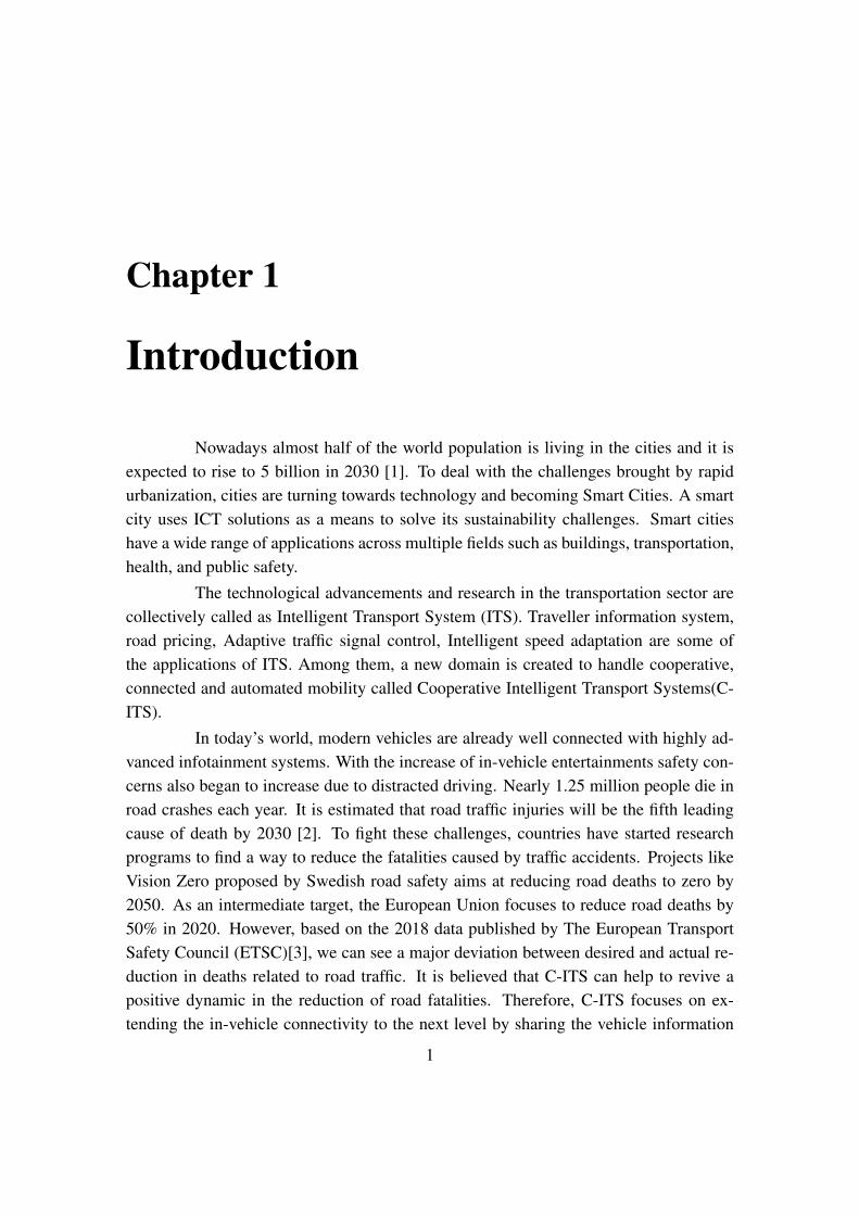
Nowadays almost half of the world population is living in the cities and it isexpected to rise to 5 billion in 2030 [1]. To deal with the challenges brought by rapidurbanization, cities are turning towards technology and becoming Smart Cities. A smartcity uses ICT solutions as a means to solve its sustainability challenges. Smart citieshave a wide range of applications across multiple fields such as buildings, transportation,health, and public safety.

The technological advancements and research in the transportation sector arecollectively called as Intelligent Transport System (ITS). Traveller information system,road pricing, Adaptive traffic signal control, Intelligent speed adaptation are some ofthe applications of ITS. Among them, a new domain is created to handle cooperative,connected and automated mobility called Cooperative Intelligent Transport Systems(C-ITS).

In today’s world, modern vehicles are already well connected with highly ad-vanced infotainment systems. With the increase of in-vehicle entertainments safety con-cerns also began to increase due to distracted driving. Nearly 1.25 million people die inroad crashes each year. It is estimated that road traffic injuries will be the fifth leadingcause of death by 2030 [2]. To fight these challenges, countries have started researchprograms to find a way to reduce the fatalities caused by traffic accidents. Projects likeVision Zero proposed by Swedish road safety aims at reducing road deaths to zero by2050. As an intermediate target, the European Union focuses to reduce road deaths by50% in 2020. However, based on the 2018 data published by The European TransportSafety Council (ETSC)[3], we can see a major deviation between desired and actual re-duction in deaths related to road traffic. It is believed that C-ITS can help to revive apositive dynamic in the reduction of road fatalities. Therefore, C-ITS focuses on ex-tending the in-vehicle connectivity to the next level by sharing the vehicle information

1

Introduction

with other vehicles and infrastructure to coordinate their movements. These co-ordinatedmovements can improve road safety, traffic efficiency by helping the driver to make theright decisions and adapt to traffic situations before-hand. In terms of economy, C-ITSimplementation helps government/organisations/individuals to save a lot of money byreducing road accidents and increasing traffic efficiency. As per annual global road crashstatistics [2], road crashes cost USD 518 billion globally, costing individual countriesfrom 1-2% of their annual GDP. Traffic congestions also take a major toll on the globaleconomy in terms of wasted time and fuel. Based on recent traffic index posted byTom-Tom [4] covering 416 cities across 57 countries on 6 continents, 239 cities showa considerable increase in traffic in 2019 compared to 2018 whereas only 63 countriesshow a reduction in road traffic. As per Inrix Annual Global Traffic Scorecard [5], UKdrivers lost an average of 178 hours a year due to congestion, costing them £7.9 billionin 2018.

To support C-ITS, the automotive industry also started integrating new tech-nologies in their vehicles to support autonomous features like Adaptive Cruise Con-trol, Lane Assist System, collision avoidance, only to mention some. Vehicles are nowequipped with precision positioning systems which help drivers to navigate through thecities by considering real-time traffic information. To support the autonomous features,vehicles are now loaded with various object sensors like Radar, LIDAR, Camera andUltrasonic sensors. With the help of these sensor inputs and their corresponding al-gorithms, Advanced Driver Assistance Systems (ADAS) help the drivers to react totheir surroundings. However, these sensors won’t be able to detect objects which arepresent beyond their horizon range especially in a blind bend corner or in the presenceof buildings or large vehicles blocking the field of view. C-ITS comes to the rescueby implementing communication between vehicles, infrastructure, and other road users.Vehicle-to-Everything (V2X) communication complements these sensors and helps thevehicle/driver to see beyond their line-of-sight.

V2X communications help to exchange useful information such as speed, head-ing, position with other vehicles (Vehicle-to-Vehicle) and/or infrastructures (Vehicle-to-Infrastructure). These data points are used by algorithms to detect possible collisions inthe future and send appropriate corrective actions to the vehicles to avoid them. Some ofthe applications of V2X communications are Lane change assist, Stationary/Slow vehicledetection, Intersection Movement Assist, Cooperative Adaptive Cruise Control. Thereare two main types of technologies used in Vehicular Communications. The first one isthe Dedicated Short Range Communication (DSRC) standard which is based on IEEE802.11p wireless communication technology. IEEE 802.11p does not require a cellular

2

Introduction

coverage, it uses onboard units (OBUs) and road-side units (RSUs) to exchange informa-tion between vehicles and infrastructure. The second one is cellular network-based usingLong Term Evolution(LTE) as a communication standard. The main aspect of vehicularcommunications is latency. For safety applications like forward collision avoidance, thelatency should be less than 100ms whereas for latency tolerant safety messages whichconcerns long-range traffic conditions like Cooperative Adaptive Cruise Control latencycan be as long as 1 second [6]. Multiple studies have been performed to analyse theperformance of both standards for safety-related applications.

As we can see C-ITS involves entities from various disciplines such as trafficsystem, communication framework, vehicle dynamics and their sensors and infrastruc-ture to process the data points. Due to the involvement of multidisciplinary entities andtheir design parameters, implementation of a comprehensive C-ITS systems becomesvery complex. Since C-ITS plays a major role in safety related applications, any issuesin the deployment may lead to loss of life. To ensure the working of different function-alities, it is suggested to test the full system in a virtual environment i.e. Simulator. Ad-ditionally, simulator helps us to identify design related issues in the early stages whichcould probably save millions if issues are identified at the deployment stage. Simula-tors are used in many fields including Vehicle Dynamics (CarMaker, Carla), Networkcommunication (ns3, OMNeT++), Traffic simulator (SUMO, Aimsun). Clearly, when itcomes to testing the functionality of full C-ITS system, multiple simulators have to talkwith each other which calls for a common framework to combine them.

The purpose of this thesis work is to create a co-simulation framework thatrepresents all components of C-ITS: vehicle connectivity, vehicle dynamics, vehicle on-board sensors, vehicle traffic, and road scenarios. The framework uses Vehicle to In-frastructure(V2I) communication model to implement the Cooperative Adaptive CruiseControl(CACC) system by taking vehicle traffic and vehicle on-board sensors into con-sideration. The network infrastructure node periodically receives Cooperative AwarenessMessages (CAM) from connected vehicles that contain information about each vehicleposition, heading, acceleration, velocity. With the received information, the infrastruc-ture node will run a trajectory-based collision avoidance algorithm which forecasts pos-sible collision between vehicles. When a collision is detected, the node will send the up-dated acceleration to the Ego car. In this way, we can analyse the performance of ADASand Communication models in safety-related applications with various traffic scenarios.

The outline that this thesis will follow is the following: The Chapter 2 cov-ers the existing solutions for the V2X communication and ADAS related applications.Furthermore, a general review of related research in the co-simulation framework is pro-vided. The Chapter 3 focuses on the co-simulation framework architecture, adopted

3

Introduction

simulation tools and the description behind the coupling of adopted simulators In theChapter 4, the simulation scenarios are presented, and an assessment of the results thathave been obtained. Finally, the Chapter 5 closes drawing conclusions on the work andpresenting some future developments.

4

Chapter 2

State of the Art

In recent years, technological innovations are playing a major role in enhanc-ing day-to-day life events in multiple areas. In particular, the automotive industry is atthe forefront among others if we consider the usage of new technologies in their prod-ucts. Nowadays, vehicles are not only a mode of transport used for transiting from pointA to point B. They are now equipped with a wide array of sensors providing multipleservices for users ranging from safety-related to multimedia services. There have beenmultiple kinds of research carried out to improve the user experience in the automo-tive domain. With the constant increase in traffic congestion, researchers figured outthat sensors in the vehicles are not sufficient to provide safety services. With the con-stant evolution of technology in the communication domain, multiple research works arecarried to provide reliable communication between vehicles. Vehicular communicationbecame the vital cog of the wheel to extend the sensing ability of vehicles beyond theirhorizon. To combine the data from vehicle sensors and communication. To provide safetravel, multiple control strategies have been developed to use the data collected throughthe communication framework and Vehicle sensors. In order to verify and improve thefunctionalities of this multidisciplinary system, researchers have also developed a fewintegrated simulators to represent the behaviour of Communication, Vehicle Dynamics,and Traffic scenarios in one combined simulation. In this section, we are going to reviewcommunication standards, vehicle dynamics and their control strategies, and researchworks related to the Co-Simulation Framework.

5

State of the Art

2.1 Vehicular Communication Standards

Vehicular communication systems are used to exchange information betweenvehicles and roadside units such as safety warnings and traffic information. Vehicu-lar communication aims at reducing road accidents and increasing traffic efficiency.Among various types of vehicular communication methods, Vehicle-to-Vehicle (V2V)and Vehicle-to-Infrastructure (V2I) used more. V2V involves exchanging informationbetween vehicles whereas V2I allows vehicles to interact with infrastructures to ex-change information between them. Vehicle-to-Everything (V2X) is a generalized rep-resentation of vehicular communications. Apart from V2V and V2I, V2X includes othermethods of communication such as Vehicle-to-Pedestrian (V2P), Vehicle-to-Roadside(V2R), Vehicle-to-Device (V2D), and Vehicle-to-Grid (V2G). A broad representation ofV2V, V2I, and V2X is shown in Figure 2.1. Dedicated Short-Range Communication(DSRC) and 4G-LTE are the widely adopted standards for the above-mentioned types ofVehicular communications. ETSI ITS-G5 is a standard adopted by the European Unionfor Vehicular Communications. It is an extension of existing communication standards,that has been modified and optimized for the dynamic automotive environment.

Figure 2.1. V2V, V2I, and V2X communications [7]

6

State of the Art

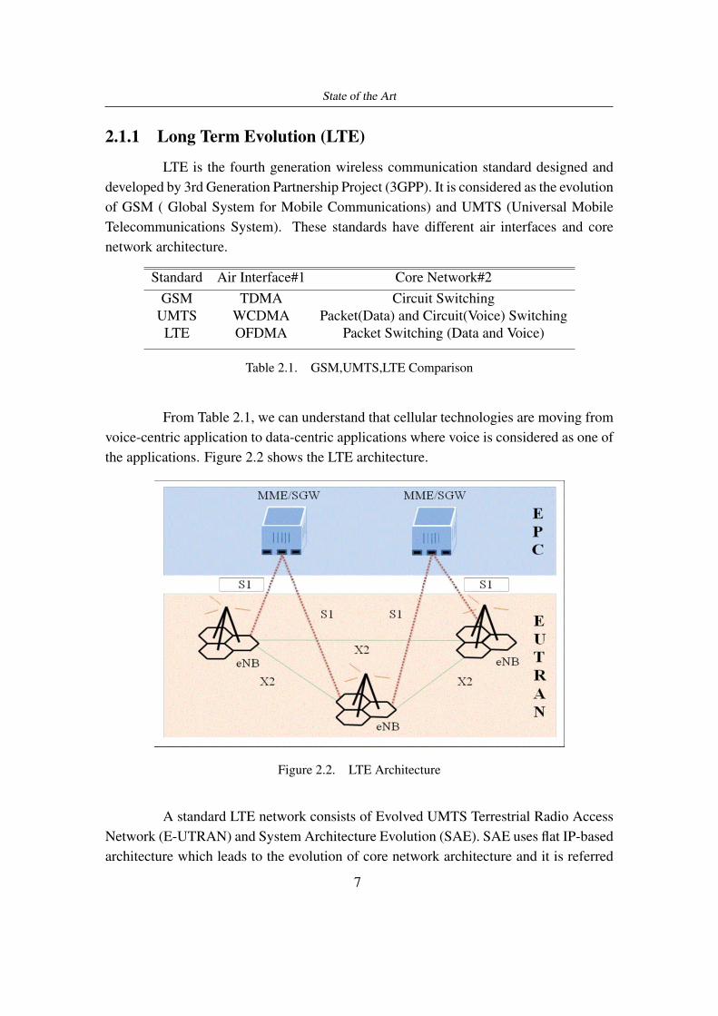
2.1.1 Long Term Evolution (LTE)

LTE is the fourth generation wireless communication standard designed anddeveloped by 3rd Generation Partnership Project (3GPP). It is considered as the evolutionof GSM ( Global System for Mobile Communications) and UMTS (Universal MobileTelecommunications System). These standards have different air interfaces and corenetwork architecture.

Standard Air Interface#1 Core Network#2GSM TDMA Circuit Switching

UMTS WCDMA Packet(Data) and Circuit(Voice) SwitchingLTE OFDMA Packet Switching (Data and Voice)

Table 2.1. GSM,UMTS,LTE Comparison

From Table 2.1, we can understand that cellular technologies are moving fromvoice-centric application to data-centric applications where voice is considered as one ofthe applications. Figure 2.2 shows the LTE architecture.

Figure 2.2. LTE Architecture

A standard LTE network consists of Evolved UMTS Terrestrial Radio AccessNetwork (E-UTRAN) and System Architecture Evolution (SAE). SAE uses flat IP-basedarchitecture which leads to the evolution of core network architecture and it is referred

7

State of the Art

to as Evolved Packet Core (EPC). EPC uses Internet Protocol (IP) as the key protocolto transport all services. This allows the network to handle data efficiently and cost-effectively.

The main units of EPC are MME, S-GW, P-GW, and HSS.Home Subscriber Server (HSS) is a central database that contains user-

related and subscriber-related information for user authentication and access authoriza-tion. It also handles functions related to mobility management, call and IP session setup.

Mobility Management Entity (MME) is responsible for handling controlsignals related to mobility and security for E-UTRAN. It is also responsible for trackingand paging idle UEs.

Serving Gateway (S-GW) handles user data traffic. It acts as an intercon-nection point between radio-side and EPC. S-GW serves UE by routing incoming andoutgoing IP packets. It acts as an anchor for the UE when it moves from one eNodeB toanother.

Packet Data Network Gateway (P-GW) helps to route packets betweenEPC and external IP networks (Packet Data Networks). It also allocates IP addresses toall UEs and enforces different policies based on their IP data traffic.

The E-UTRAN is comprised of UE’s (user equipment) and eNodeB’s (evolved-NodeB’s). Its radio interface is called as E-UTRA, the Evolved Universal TerrestrialRadio Access. The eNodeB acts as a base station which helps UE to connect with theLTE network. eNodeB uses Uu, X2 and S1 interfaces to communicate with UE, othereNodeBs and EPC respectively. In the previous generation, NodeB’s are controlled bya Central Radio Network Controller (RNC). The RNC is responsible for the allocationof radio resources to NodeB’s and their mobility. In LTE, eNodeB has to handle allair interface communications, radio resource allocation, header compression, security,modulation, interleaving, handover and retransmission control. The absence of centralcontroller and distributed radio control functions help LTE to provide a Round Trip Timetheoretically lower than 10 ms, and transfer latency in the radio access up to 100 ms [8].This is beneficial for safety-related applications especially vehicular communications.

Device to Device Communication in LTE

To support safety-critical communication systems, 3GPPP updated the LTEarchitecture to include the Proximity-Based-Services (ProSe) that enable direct com-munication between two UEs, also known as Device-to-Device (D2D) communication.Reserved LTE resources are used for D2D communication. It allows interaction betweenUEs nearby using a direct link instead of communicating with other UE using a base

8

State of the Art

station or the core network. Due to the reduced signal traverse path, it can achieve lowlatency requirements demanded by safety-related applications. ProSe introduced to workin places where coverage is not guaranteed. The figure 2.3 shows the ProSe communica-tion scenarios [9].

Figure 2.3. ProSe Communication Scenarios

In Coverage scenario, ProSe communication resources are allocated by theLTE network. To reduce the cellular traffic interference and optimize the ProSe com-munication, the network either assigns a pool of resources selected by the UE or assignsspecific resources to the transmitting UE. In out of coverage scenarios, control from thenetwork is not possible. However out-of-coverage doesn’t mean there is no eNodeB inthe range. There is a possibility of eNodeB presence from a different cellular networkprovider. In partial coverage scenario, with pre-configured values, out-of-coverage UEcan communicate with UE in coverage where it uses the resources from the eNodeB.

Figure 2.4. LTE ProSe Architecture [9]

9

State of the Art

Figure 2.4 shows interfaces used to communicate between LTE modules. Whena UE wants to use the ProSe functionality, it should first contact ProSe function throughthe PC3 logical interface for authorisation and security paraments. After receiving se-curity parameters through the PC3 interface, UE initiates discovery procedures to lookfor another ProSe enabled UE nearby using the PC5 interface. When two or more UEshave discovered each other, they can initiate a direct link between them. Like conven-tional cellular networks, usage of Uplink and Downlink to exchange data between UEand eNodeB is extended and adopted in ProSe communication to exchange informationbetween UEs. The physical interface between ProSe enabled UE’s is called SideLink(SL). Since it’s a safety-related communication, SL transmissions are based on multicas-ting so, transmitters do not receive any feedback from receivers. ProSe communicationwas further enhanced in release 13 by introducing a multi-hop D2D network where UEsact as a relay between eNodeB and other UEs.

LTE based V2X

With D2D technology as a steppingstone, 3GPPP has introduced LTE-basedVehicle to Everything (V2X) service in its 14th release. User equipment involved inthe V2X service could be pedestrian hand-held devices, Roadside Units (RSU), Infras-tructure nodes or vehicles. V2X messages can be sent either using the Uu interfacewhich represents the radio interface between eNodeB and UE or as direct communica-tion between UE’s using the PC5 interface. Using LTE-Uu interface, UE can either trans-mit/receive unicast V2X messages or transmit a unicast message to eNodeB and receivea broadcast message via Multimedia Broadcast Multicast Service (MBMS) delivery. Us-ing PC5 UE can send/receive V2X messages using SideLink. Three main scenarios ofLTE based vehicular services are discussed in the “Feasibility Study on LTE-based V2XServices” [10]

In the first scenario as shown in 2.5, V2X operations are handled only by thePC5 interface. That means D2D is the only way of exchanging messages. For V2I,either vehicle can transmit to RSU or RSU can transmit data to the group of vehiclesusing SideLink.

In the second scenario as shown in 2.6, the V2X operation can be handled onlyby the Uu interface. In this case, all the V2X messages are sent through eNodeB. ForV2I, the vehicle sends a V2X message to eNodeB using Uplink where eNodeB takescare of sending the message to the destination UEs in the local area by downlink.

In the third scenario as shown in 2.7, it’s a combination of the above two sce-narios where it supports V2V operation using both Uu and PC5 interface. A vehicle

10

State of the Art

Figure 2.5. Scenario 1 V2I Operation

Figure 2.6. Scenario 2 V2I Operation

Figure 2.7. Scenario 3

11

State of the Art

UE sends a message to other RSU type UE using the PC5 interface. RSU UE sends theV2X message to E-UTRAN in an uplink. E-UTRAN receives the V2X message fromthe RSU UE and then transmits it to a group of UEs in close vicinity using downlink.In this scenario, E-UTRAN performs both uplink and downlink for V2X messages anddownlink, E-UTRAN used a broadcasting mechanism.

The evolutions in LTE released by 3GPPP lead to considering LTE as a possi-ble solution for safety-critical communications in the ITS field.

2.1.2 Dedicated Short Range Communication (DSRC)

Dedicated short-range communication (DSRC) is a wireless communicationtechnology developed by the US Department of Transportation (USDOT) which playsa major role in the Intelligent transportation system (ITS). It is designed to support avehicle to communicate with other vehicles and/or infrastructures. The characteristicsof DSRC like low latency, secure, fast network acquisition, and handover, network re-liability against interference in adverse weather conditions make its ideal for vehicu-lar communications. DSRC can support both vehicle-to-vehicle (V2V) and vehicle-to-infrastructure (V2I) type of communications. On-Board Units (OBU) acts as transpon-ders in vehicles where Road-side Units (RSU) acts as fixed access points and usuallypermanently mounted along the roadside. Both units are equipped with a satellite posi-tioning system which is mainly used for time synchronisation between devices. In V2V,DSRC allows vehicles to communicate with each other especially the exchange of safety-related messages. In V2I, a vehicle OBU communicates with surrounding infrastructureequipped with an RSU. This can be used to collect tolls, transferring multimedia, andalso safety-related messages like road conditions. The basic functionalities handled byDSRC is shown in 2.8

Figure 2.8. DSRC Communication [11]

12

State of the Art

The PHY and MAC layers of DSRC are defined by IEEE802.11p while DSRCupper layers are handled by the IEEE 1609 family of standards, which is commonlyreferred to as Wireless Access in Vehicular Environment (WAVE). The IEEE 802.11pstandard is a part of the 802.11(Wi-Fi) family which is developed to support vehicularcommunications.

Figure 2.9. WAVE Protocol Stack [12]

WAVE Physical Layer

As shown in Figure 2.9, the IEEE802.11p standard is used to represent theWAVE PHY layer. The IEEE802.11p PHY layer is similar to the IEEE 802.11a PHYlayer as shown in Table 2.2, where both the version operates at the same frequency rangeof 5 GHz, specifically 802.11p operates between 5.850 and 5.925 GHz. This is reason-able because changes in the MAC layer are mostly software related but major changes inthe Physical layer could demand entirely new wireless air-link technology. The modula-tion technique adopted by 802.11p as well as 802.11a is Orthogonal Frequency-DivisionMultiplexing (OFDM). An OFDM signal consists of several closely spaced modulatedcarriers. Usually, when signals are transmitted close to one another they should be spacedout so that the receiver would be able to separate the signals and there should be a guardband between them to prevent the interference. However, subcarriers in OFDM are or-thogonal to each other which prevents the cross-talk between subchannels and the needfor inter-carrier guard bands. This reduces complexities in the design of the transmitterand receiver.

13

State of the Art

IEEE 802.11a IEEE 802.11p

Data Rate (Mbps)6, 9, 12, 18,24,36, 48, 54

3, 4.5, 6, 9,12, 18, 24, 27

ModulationBPSK, QPSK,

16-QAM, 64-QAMBPSK, QPSK,

16-QAM, 64-QAMODFM Symbol Duration 4.0 µs 8.0 µs

Guard Period 0.8 µs 1.6 µsOccupied Bandwidth 20 MHz 10 MHz

Frequency 5 GHz ISM band 5.850-5.925 GHz (dedicated)

Table 2.2. Comparison between IEEE 802.11a and IEEE 802.11p [13]

IEEE 802.11p uses 10 MHz wide channel while IEEE 802.11a uses a 20MHzwide channel. The main reason for this change is to address increased RMS delay spreadin the vehicular environment. This change also prevents the inter-symbol interferencesby having longer guard intervals compared to IEEE802.11a. The 75MHz band in IEEE802.11p is divided into 7 channels with 10 MHz width, One Control Channel (CCH)and 6 Service changes (SCH). CCH is located at the centre whereas SCH are at thesides. CCH used solely for security communications. SCH can be used to transmit allinformation with lower priority. It is possible to combine two SCHs into one 20 MHz-wide SCH thus doubling the data rate.

WAVE Lower MAC

Similar to WAVE PHY layer, the IEEE 802.11p MAC layer represents WAVElower MAC which is again a modified version of previous standards to support vehicularnetworks. WAVE Lower MAC includes some of the features from IEEE 802.11e suchas channel coordination and Enhanced Distributed Channel Access (EDCA). EDCA is amodified version of Distributed coordination function (DCF) which operates on the con-tention period. EDCA adopts contention-based channel access and uses Carrier SenseMultiple Access with Collision Avoidance (CSMA/CA). CSMA/CA tries to reduce thefrequency of packet collisions occurred due to simultaneous transmissions. It followsthe idea of the “Listen Before Talk” (LBT) principle. After receiving the packet fromupper layers, a node transmits only if the medium is free for an amount of time equal toan AIFS (Arbitration Inter-Frame Space). If the medium is not free, the node waits fora random back-off time before transmitting. The main feature of EDCA is traffic differ-entiation using multiple access categories. Each access category has a different accesspriority, back-off time interval. IEEE 802.11p MAC categorizes the messages based on

14

State of the Art

its priority and allocates proper access parameters for safety-related messages to ensuretheir quick and successful transmission. Vehicular safety-related applications demand in-stantaneous data exchange capabilities and do not have enough time to perform standardauthentication and association to join a BSS. The WAVE standard introduces a new BSStype: WBSS (WAVE BSS). A station forms a WBSS by first transmitting an on-demandbeacon. The demand beacon contains the information like services offered by WBSSand necessary configuration information to become a member of WBSS. Based on theinformation provided by the beacon, a station can decide to join a WBSS with no furtherinteractions. This reduces the necessity of association and authentication processes byoffering extremely low overhead for the WBSS setup.

WAVE Upper MAC

The WAVE upper MAC layer defined by the IEEE 1609.4 standard which isresponsible for the multi-channel coordination. WAVE has two different channel types:Control Channel (CCH) and Service Channel (SCH). IEEE 1609.4 specifies how to usethem using Channel Coordination. Channel Coordination is designed to support data ex-changes involving one or more switching devices with alternating operation on CCH andSCH channels. A single radio device can use different channels by alternating betweenSCH and CCH with 50ms dedicated to each of them. Time is divided into sync intervals.In 1 sec, there are 10 sync intervals with each sync interval lasting for 100ms. Each syncinterval composed of A CCH interval and A SCH interval. A guard interval is present atthe beginning of each channel interval (CCH interval or SCH interval) which is used toaccount for radio switching and timing inaccuracies among different devices. The syn-chronization function uses UTC (Coordinated Universal Time) as the common time basefor CCH and SCH intervals which can be obtained by Global Positioning System (GPS)receivers. GPS receivers typically provide a precise one pulse per second (PPS) UTCsignal with an error of less than 100 ns, and these precise one PPS signals can be usedfor timing and synchronization. Timing Advertisement frame can be used by the nodeswithout local timing source. Those devices use the timestamp field in the Timing Ad-vertisement frame as an input to estimate the UTC. Nodes that are not synchronized canonly monitor the CCH channel for safety messages. The Control Channel (CCH) is usedto transmit management packets and WAVE Short Messages (WSM) carried by WAVEShort Message Protocol (WSMP) whereas Service Channel (SCH) is used to transmitall packet types, including IPv6 packets. The type of access given to CCH and SCHchannels are categorized into three types: continuous channel access (CCH or SCH), al-ternating access between two channels (CCH/SCH or two SSHs),and immediate channel

15

State of the Art

access.

WAVE Short Message Protocol (WSMP)

DSRC protocol stack is created to support both standard and vehicular com-munications. For non-safety IP based messages, default protocols such as the IP (InternetProtocol) and the TCP (Transport Control Protocol) or UDP (User Datagram Protocol)can be exploited by the network and transport layer respectively. Due to their over-head, these protocols are not suitable for V2X communication scenarios. WAVE ShortMessage Protocol (WSMP) is a networking protocol specifically designed for V2X com-munications. WSMP also allows the applications to choose the desired physical char-acteristics that should be used in transmitting the messages. The PHY and MAC layerread the contents of each packet and adjust the radio power, data rate accordingly beforetheir transmission. The WAVE Management Entity (WME) is responsible for the man-agement of networking services function, provided by the IEEE 1609.3 standard. Thisentity takes care of frame queuing, priority channels and handling of safety messages.Server applications registers with WME using a Provider Service Identifier (PSID) anduser applications register their interests using WME. Based on the PSID, WSMs are de-livered to the respective application(s). If the application-service is not interested in thePSID value of a received WSM, the receiver ignores the message. WAVE Security En-tity (WSE) is responsible for the management of data encryption mechanisms and keymanagement. WSM follows IEEE 1609.2 standard, that defines the format for securemessages. Since WSMs play a major role in Vehicular safety-related applications, pro-tecting them from cyber-attacks is very crucial.

2.1.3 V2X Messages

C-ITS aims at creating a co-operative vehicular environment where vehicles takeactions based on the information gathered from surrounding traffic actors and infrastruc-tures. C-ITS applications are categorized into three categories: safety, traffic efficiency,infotainment. The communication strategy of most common C-ITS applications can begrouped into two types: Periodic status exchange and Asynchronous notification [14].Periodic status exchange handles messages that are sent periodically to announce a vehi-cle’s location, speed, the status of RSU’s. It can be used by traffic efficiency-related ap-plications for monitoring vehicle movements. It can also be a part of safety applicationswhere vehicle information can be used to predict potential vehicle collisions in the fu-ture. Asynchronous notification is generated to inform the occurrence of specific events.It’s mostly used by safety applications to broadcast information about road accidents,

16

State of the Art

slippery roads and so on. To standardise the application support messages, ETSI hasdefined two basic messaging services: Cooperative Awareness Basic Service for Coop-erative Awareness Messages (CAM), and the Decentralized Environmental NotificationBasic Service for Decentralized Environmental Notification Message (DENM).

Cooperative Awareness Messages (CAM)

The Cooperative Awareness Message (CAM), defined in the ETSI EN 302637-2, can be considered as the heartbeat messages of the ITS scenarios where nodesperiodically send their information to the neighbouring nodes. Some of the informationincluded in CAM’s are heading, acceleration, intended route, timestamp. By gatheringinformation from CAM’s, the vehicle can track the movements of surrounding vehiclesand look for any potential collision occurrence in the future. If vehicles are in a collisioncourse, cooperative manoeuvres are enabled to avoid the collision.

Figure 2.10. CAM Message Structure

The figure 2.10 represents the CAM message structure. The header containsdetails of the message such as version, message identifier and generation time. Thecontainers in the mandatory section handle the information like sender ID, type of ITSstation, position, heading. Some other optional parameters can be included by the ITSstation based on the recommendations made by the standard. The frequency of the CAMmessage can be varied from 10Hz to 1Hz. The dynamic generation of CAM is alsopossible by considering the change of position and speed of the vehicle.

17

State of the Art

CAMs are generated by the CAM Management and messages are passed to lowerlayers when any of the following conditions satisfied:

• the maximum time interval between CAM generations: 1 second;

• the absolute difference between current heading (towards North) and last CAMheading > 4°;

• distance between the current position and last CAM position > 5 m;

• the absolute difference between current speed and last CAM speed > 1 m/s; Thesegeneration rules are checked every 100 ms.

Distributed Environmental Notification Message (DENM)

DENM service generates a DENM based on the occurrence of certain eventsdefined by the application. It aims to alert other vehicles about the event which has animpact on road safety. According to standard, an event contains the following details:event type, position, detection time, the destination area, transmission frequency. Theapplication sends the event details to the DENM service which starts transmitting DENMmessages periodically over the specified destination area. It also notifies the DENMservice about any changes in the events. Once the time is expired or the applicationcancels the event, the DENM service stops transmitting the DENM messages. The figure2.11 represents the DENM message structure.

Figure 2.11. DENM Message Structure

18

State of the Art

2.2 Vehicle Dynamics

In this section, we are going to talk about the basics of Vehicle Dynamics. In asimple way, a vehicle is broadly classified into three modules: power, chassis, and body.The power module is to take care of the engine, gearbox, axles, etc. The chassis mod-ule includes multiple subsystems such as suspension, steering, tires, and so on. Vehicledynamics focuses on representing all these modules, subsystems, interactions with theexternal forces as a mathematical model. The main aim of vehicle dynamics is to studythe safety, and comfort of the vehicle occupants by understanding the behaviour of thevehicle under different scenarios through the mathematical models. The vehicle dynam-ics play an important role in the development of a vehicle.

Figure 2.12. Basic representation of Vehicle Dynamics

In a simple mathematical model as shown in Figure 2.12, the definition of thevehicle is not anymore in the form of subsystems instead of vehicles that are definedin terms of mass, moment of inertia, stiffness, damping, compliance, etc. Vehicle-roadcoupling is an important aspect of vehicle dynamics. The input can be a wide varietyof actions performed by a driver such as steering input, braking, accelerating throughrespective subsystems whereas outputs represent the quantities related to safety, comfortsuch as braking distance, which is the main aspect in safety, acceleration/decelerationthat deals with the comfort of the passenger. A mathematical model should be complexenough to consider driving dynamics such as manoeuvres, self-steer behaviour, oscilla-tory motion behaviour, load shifts, and so on. The complexity of a mathematical modelincreases with the Degree of Freedom (DOF). Vehicle Dynamics is broadly classifiedinto three categories:

• Longitudinal Dynamics: forces in the longitudinal direction. e.g. acceleration;

• Lateral Dynamics: forces in the lateral direction. e.g. cornering, handling, stability;

• Vertical Dynamics: forces in the vertical direction. e.g. vibration, road/tire contact.

For this thesis, we are only going to see about longitudinal dynamics and control.

19

State of the Art

Longitudinal Dynamics

Longitudinal Dynamics study about the forces and motions in longitudinal di-rection. It can be used to predict top speed, acceleration and braking performances,gradeability, fuel consumption. Figure 2.13 shows types of forces that act on a vehicle inan inclined road.

The front and rear longitudinal tire forces are generated from the vehicle powertrain. Based on Newton’s second law, tire forces should overcome the resistance forcessuch as aerodynamic force (Faero), gravitational force (mgsinα) and rolling resistances(Rx f ,Rxr). The imbalance between them decides the resultant longitudinal accelerationof the vehicle.

Figure 2.13. Longitudinal Vehicle Model

A longitudinal model can be represented by:

mx = Fx f +Fxr −Faero −Rx f −Rxr −mgsinα (2.1)

where:

• mx is the vehicle acceleration,

• Fx f ,Fxr are front and rear forces respectively,

• Faero represents the aerodynamic forces,

• Rx f ,Rxr are front and rear rolling resistance,

• mgsinα represent the gravitational force on inclined surface.

20

State of the Art

We can simplify the model by combining tire forces, rolling resistance forces, roadinclination angle approximation to achieve a basic dynamic model for the longitudinalmotion.

mx = Fx −FL (2.2)

FL = Faero −Rx −mgα (2.3)

where:Fx represent traction force, FL represents the total resistance forces acting on the

vehicleWe can develop different mathematical models to represent each of the forces

mentioned in the equation 2.2 based on our requirements.

2.3 Control Strategies

The automotive industry is transitioning from hardware- to software-definedvehicles, the relevance of software for core technology trends is increasing rapidly [15].To provide safe and comfortable driving, cars are now equipped with multiple devicessuch as RADAR, camera, ultrasonic sensor, lidar, positioning systems to understand thesurroundings of a vehicle. Sensors play a major role to fulfil the future requirements ofpartially and fully autonomous vehicles. For example, RADAR has introduced multiplesafety applications in the automotive industry. RADARs have the capability to detectobjects in a wide area based on their operation range. Apart from these sensors, we canalso acquire vehicle data from the Inertial measurement unit (IMU), and internal buses(Controller Area Network (CAN)). With the abundant availability of data giving infor-mation about the vehicle surroundings as well as the current vehicle behaviour, multiplesafety applications have been created to process and analyse the data efficiently. Thoseapplications are collectively called as Advanced Driver Assistance Systems (ADAS).ADAS plays a preventive role in mitigating crashes and accidents by providing a warn-ing or additional assistance in steering/controlling the vehicle. ADAS is considered as anevolution of Driver Assistance Systems (DAS). DAS uses data from sensors measuringvehicle internal values such as velocity, acceleration or wheel rotational velocity. A fewnotable DAS based applications are Anti-lock Braking System (ABS), the ElectronicStability Control (ESC) and the Traction Control System (TCS). Some of the ADASbased applications are Adaptive Cruise Control (ACC), Autonomous Emergency Brak-ing (AEB), Electronic Stability Control (ESC), Lane Keeping Assist (LKA). However,

21

State of the Art

ADAS related applications can only react to the objects that are in the range of the sen-sors.

Figure 2.14. RADAR Types: LDR- Long Range RADAR; MDR-Mid Range RADAR;SDR-Short Range RADAR [16]

For example, RADAR cannot detect the slow-moving vehicle that presents be-fore the target vehicle and its range depends on the type of RADAR used as shown inFigure 2.14. This kind of scenario can potentially create a collision between vehicles.With the advancement in V2X technologies, we can overcome these situations. CollisionAvoidance, Cooperative Adaptive Cruise Control (CACC) are some of the applicationsthat consider data from on-board sensors as well as data received through communi-cation frameworks. According to, human errors are the critical reason for 94% of carcrashes[17]. Among them, 41% due to recognition error which includes driver’s inatten-tion, internal and external distractions, and 33% are caused by decision errors such asdriving too fast for conditions, illegal manoeuvre, misjudgement of the gap [17]. Severalstudies showed that ACC and CACC help to improve traffic efficiency by reducing thenumber of accidents, increasing vehicle average velocity. According to the study, CACCalso increases the string stability in platooning, thus improving the traffic flow.

2.3.1 Adaptive Cruise Control

Adaptive Cruise Control (ACC) is an enhancement of conventional CruiseControl. The conventional Cruise Control can only maintain the user set speed by ac-celerating/decelerating the vehicle. The Driver has to intervene if the preceding vehiclevelocity is lower than the user set speed. ACC is developed to overcome this drawbackby adapting the vehicle’s speed to the traffic environment. The detection of the preceding

22

State of the Art

vehicle is usually handled by RADAR based system. The RADAR gives two data pointsas input to ACC: ds represents the relative distance between the own vehicle and targetvehicle; dv represents relative velocity between own vehicle and the target vehicle. Ifa slower moving vehicle is detected, the ACC system decelerates the vehicle to main-tain the time gap between the target vehicle and the host vehicle. If there is no vehiclepresent in the range of the RADAR, the vehicle accelerates to its set cruise speed. In thisway, ACC can control the vehicle without the intervention from the driver. However, thedriver can de-activate ACC at any time by giving any kind of input to the system. Figure2.15 shows simplified ACC working model.

Figure 2.15. ACC Working Model

2.3.2 Automatic Emergency Braking

The purpose of Autonomous Emergency Braking (AEB) is to avoid or reducethe impact of a collision which generally caused by decision errors made by the driver.AEB requires two inputs: the surrounding vehicle’s information and its vehicle state.The surrounding vehicle’s information is gathered by RADAR and/or Camera.The AEBworking principle can be grouped into four steps [18]:

1. Identify critical situations: AEB finds a potential collision situation by combiningthe information from exteroceptive sensors and own vehicle states.

2. Prepare the braking system and warn the driver: After the identification of apotential collision situation, AEB starts filling the brake circuit with fluid. Thishelps the system to reduce the preparation time to apply the brake, in turn, reducingthe braking distance. It also warns the driver about the possible collision throughvisual and auditory warning-signals.

23

State of the Art

3. Soft braking: if the driver didn’t respond to the warnings and potential collisionevent is still valid, then AEB starts applying the brake with a deceleration requestup to -4 m/s2.

4. Hard autonomous braking: if the collision is imminent and the driver is not re-sponding to any warning provided earlier, AEB gets activated and it takes control ofthe brake system and apply the emergency brake with deceleration forces up to -9.8m/s2 . AEB tries to avoid the collision or at least reduce the impact of a collisionby applying the emergency brake.

2.3.3 Collision Avoidance

Collision detection is the first and foremost step to avoid a collision. In thisversion of the Collision Avoidance algorithm, an Infrastructure gathers information ofall the vehicles around it through V2I communication systems. A generic trajectory-based algorithm is used to detect any vehicle that is on the collision course with another.The algorithm requires velocity, heading angle, position of the vehicles to detect a poten-tial collision occurrence. Since it’s a trajectory-based algorithm, it calculates the futureposition of each vehicle using these inputs. It just assumes the future possible positionwith the current velocity and heading angle. As of now, the algorithm has calculated theposition of all vehicles for the next 5 seconds. At this point, it calculates the distancebetween each vehicle position with other vehicles. If the distance between any vehicleis less than the predefined threshold, those vehicles are considered to be in a collisioncourse with each other. To avoid this collision, a corrective action like change in accel-eration is communicated to one of the vehicles that are identified to be in the collisioncourse with another vehicle. The choice of vehicle could be based on multiple parameterslike vehicle priority, distance, comfort

2.3.4 Co-operative Adaptive Cruise Control

With the technological advancements in V2X communications like DSRC, ahost vehicle has the opportunity to communicate with other vehicles and/or infrastruc-tures to get information about the surrounding environment. ACC can be co-operative byusing information received through communication systems and react to the objects thatare beyond the horizon of driver and sensors perception. Co-operative Adaptive CruiseControl (CACC) exploits sensor data, host vehicle data, over the air data from surround-ing vehicles and/or infrastructures to control the vehicle acceleration, as shown in Figure2.16.

24

State of the Art

Figure 2.16. CACC Functional Elements [19]

Through V2X communications, CACC can get frequent updates about the sur-rounding vehicle behaviour which help to maintain the desired time gap between vehi-cles without oscillations and respond quickly to any changes in the preceding vehiclebehaviour. Due to the fast response, we can also reduce the desired time gap and followthe vehicle closely without compromising driver safety. One of the main applications ofCACC is Platooning. A platoon is a group of vehicles that travel together. The lead vehi-cle changes its speed and direction where other vehicles follow their preceding vehicle.

2.4 Literature Review

The goal of co-simulation frameworks is to combine the strength of multi-ple simulation tools and to develop a solution for real-world problems. There are fewintegrated simulators developed to achieve the interaction between traffic and networksimulation environment; traffic flow and vehicle dynamics; Control, Communication,and Traffic flow. In this section, we are going to discuss the existing Co-Simulationframeworks and their functionalities.

The work made by Dmitry Kachan [20] integrates ns3 with MATLAB/Simulinkto handle dynamic vehicle motion and wireless communication. MATLAB is used tocreate dynamic traffic movements where ns3 is used to simulate wireless communication

25

State of the Art

networks. Socket programming is leveraged to combine MATLAB/Simulink and ns3. Atthe end of each simulation step, Simulink does the calculations of future possible eventsand MATLAB sends those instructions to ns3 through a socket connection. And ns3executes those instructions until the expiration of the simulation step. At the end of thens3 simulation step, it sends the report to MATLAB. On each simulation step both sim-ulators exchange messages which include status information for each node. The figure2.17 shows the Interaction between ns3 and MATLAB. This work mainly focusses oncreating an interface between two simulators but didn’t define any control strategies anddidn’t test the framework by using different vehicle movements or communication sce-narios. But we have created a framework that combines multiple simulators that includesmobility modelling and also tested our framework with different traffic scenarios.

Figure 2.17. Interaction between ns3 and MATLAB [20]

The framework made by Jakob Kaths[21] et.all involves IPG CarMaker andSimulation of Urban MObility (SUMO) for integrating microscopic traffic simulationand vehicle dynamics simulation. The integrated framework is developed with MATLAB-Simulink as a mediator. CarMaker for Simulink helps CarMaker to communicate withSimulink whereas, for traffic flow simulation, the programming interface TraCI4Matlab

26

State of the Art

allows the interaction with SUMO through MATLAB/Simulink. In the simulation, SUMOis used to simulate all vehicles including Ego car from CarMaker. The position of Egocar is updated in SUMO through the TraCI command “moveToVTD”. During the simu-lation, the IDs, positions, and speeds of the surrounding vehicles are retrieved and sentto CarMaker to update them within the CarMaker environment. They have tested theirframework by using high and low traffic volumes from SUMO and ACC implemented toadapt the speed of Ego Car in CarMaker using ADAS functionalities. Their main focusis to analyse the vehicle dynamics based on the traffic flow. While we have created aframework that focuses on vehicular safety applications by identifying and avoiding col-lisions through CACC as well as ACC. We have also used CarMaker for both traffic andADAS functionalities.

The work done by Chenxi Lei[22] integrates SUMO, Simulink and OMNeT++2.18 for analysing String Stability. The term “string stability” means that any non-zeroposition, speed, and acceleration errors of an individual vehicle in a string do not amplifywhen they propagate upstream.

Figure 2.18. Simulation Experimental Structure [22]

Each simulator is devoted to one specific functionality. Simulink handles Vehi-cle behaviour including the ACC and CACC, SUMO takes care of Mobility, OMNeT++with MiXiM simulates communication networking behaviour. To creating a couplingbetween SUMO and Simulink, Real-Time Workshop tool in Simulink is used to convertthe Simulink model into a C++ shared library and called in the source code of SUMO.The bidirectional coupling between OMNeT++/MiXiM and SUMO is achieved through

27

State of the Art

TRAffic Control Interface (TraCI) by transmitting TCP messages. In their work, MiXiMcollects information of all nodes(vehicles) at every simulation step and send it to SUMOthrough TraCI where acceleration data is given as input to the Simulink model for calcu-lating the next acceleration and velocity. Based on that, vehicles are moved to SUMO.The new trace is sent back to MiXiM where it moves the communication nodes accord-ing to the vehicles’ position information from SUMO. They have used the frameworkto analyse String Stability by varying time headway, beacon rate, packet loss ratio andACC versus CACC. As we said earlier, his main focus is to study the string stabilitywhich impacts the platooning related applications. They also struggled to switch be-tween ACC and CACC based controller while we have successfully implemented thesame. We can switch between ACC and CACC controllers by considering the desiredacceleration calculated by them.

Amr Ibrahim et. all [23] made a co-simulation framework consisting of MAT-LAB for control algorithms, ns3 for network simulation and SUMO for traffic behaviour.This framework runs in two different systems where MATLAB, SUMO runs on the Win-dows operating system and ns3 runs on a Linux virtual machine. MATLAB acts as aninterface between ns3 and SUMO. The TCP connection is established between SUMOand MATLAB using TraCI (Traffic Control Interface). Socket programming is used forthe TCP connection between MATLAB and ns3. The co-simulation framework is shownin figure 2.19.

Figure 2.19. ns3 and SUMO Interaction through MATLAB [23]

During the simulation, MATLAB retrieves the vehicle’s information such asthe current position, speed from SUMO. The vehicle information is forwarded to ns3through TCP socket connection where ns3 simulates the packet broadcast of each ve-hicle through a constant velocity mobility model. The packet reception information ofeach node is stored in the lookup table. MATLAB accesses the lookup table and runsthe control algorithm to define the new position, velocity. This new vehicle informationis updated in the SUMO through TraCI. This framework is used to validate different

28

State of the Art

platooning setups. Apart from the choice of simulators, their main focus is to study theimpact of Packet Reception Ratio and delay on the overall platoon performance. Theyhave executed their framework for different traffic densities in a realistic highway sce-nario. We have tested the framework for different scenarios in an ideal communicationenvironment without considering channel load. We have also used LTE based com-munication model while they have employed WAVE standard to communicate betweenvehicles. To communicate between ns3 and MATLAB, we have exploited the MATLABcommands and Sockets while they have used only TCP/IP sockets to transfer informa-tion. Using MATLAB commands gave us flexibility to transfer vehicle information inmultiple formats which is not possible with TCP Socket.

Figure 2.20. ns3 and VISSIM Interaction through MATLAB [24]

Apratim Choudhury et.all [24] developed a framework with VISSIM (for traf-fic simulations), MATLAB and ns3. VISSIM and MATLAB communicate through VIS-SIM’s COM interface in a Windows host machine. ns3 is installed in a virtual Linuxmachine connected via virtual network. The sockets API is used for the communicationbetween MATLAB and ns3. Figure 2.20 shows the framework developed by Apratimet. all. This simulation platform is used to model platoon control algorithms, the controlobjective of this algorithm is to compute the necessary acceleration that the car needs tofollow the leader. The waypoint mobility model is used in ns3 for moving nodes. There-fore, to move from point to another point, a node requires an origin and a destinationwaypoint. To get these waypoints, VISSIM has to run the simulation beforehand andsend the origin and destination waypoint to ns3. Thus, control action is implemented inVISSIM with an approximate delay of 0.1 seconds. They have used 802.11p standardto establish V2V communication model in order to exchange CAM messages betweenvehicles. We have used LTE standard to establish V2I communication to implement theCACC algorithm. Their focus is on the platooning related applications while we focusedon the enhanced CACC system that predicts the possible collision in the future.

29

State of the Art

Based on the research made on Co-Simulation frameworks, we can see thatmost of them used Sumo as their traffic simulator and used TRACI to connect with othersimulators, ns3 or OMNeT++ as network simulator, Simulink or CarMaker as vehicledynamics simulator. Among them, Dmitry Kachan framework depends on the creationof new C++ methods to make ns3 communicate with an external simulator. i.e. MAT-LAB. We have to change some core functionalities of ns3 to achieve the connectivitybetween ns3 and MATLAB. Whereas framework introduced by Lei converts Simulinkmodel into C++ code to create a communication between SUMO and OMNeT++. Theintroduction of new methods and the conversion of a base model has two disadvantages.One, we lose the flexibility of the framework. If we want to add new functionality to theframework like adding vehicle dynamics which doesn’t exist in both of the frameworks,we have to either use simulators which are compatible to the framework or convert theexisting simulation model into a model that is suitable for the framework. Second, whileconverting models, we lose some core functionality of the base simulator like while con-verting Simulink code Lei loses some of the functionalities that are only available inSimulink. While the framework proposed by Jakob studied only the behaviour of thevehicle in various traffic scenarios using vehicle ADAS functionality. The frameworkdidn’t consider the usage of connected vehicles in the traffic scenarios. With the auto-motive world moving toward connected vehicles, this seems to be a big drawback of thisframework. While Apratim and Amr Ibrahim, focuses on creating a communication be-tween vehicles but they didn’t consider the dynamics of the vehicle. While introducingthe communication between the vehicles, we have to consider also the response of thevehicle which helps the framework to create a virtual simulation close to real-world envi-ronment. In the proposed framework, we have addressed all the disadvantages expressedby the above frameworks. We have used CarMaker to study the dynamics of the vehicle,to emulate traffic scenarios and vehicle sensors, and ns3 for creating communication be-tween the vehicles. Moreover, we have combined these simulators using a Python-basedinterface which doesn’t require conversion any core simulators. In this way, the proposedframework, able to use full functionalities of all the simulators and also able to replicatea real-world environment in a virtual simulation. As a control strategy, we have usedenhanced CACC which makes the vehicle follow the preceding car as well as to avoid acollision that’s going to happen in the future using a trajectory-based algorithm.

2.5 Simulation Tools

The objective of this paper is to develop a simulation framework that repre-sents all the following system components realistically: vehicle connectivity, vehicle

30

State of the Art

dynamics, vehicle on-board sensors, vehicle traffic, and road scenarios. To achieve theproject objective, the framework has to integrate multiple simulators, each devoted to therepresentation of one specific component.

2.5.1 Network Simulator

Network simulators are used to implement and analyse the behaviour of net-works before deploying in the real world. Network simulators can evaluate the perfor-mance of network frameworks under dynamic changes e.g., the traffic conditions, thecommunication channel conditions. In this framework, Long Term Evolution is usedfor receiving information about the surrounding vehicles. The operation of the LTE ismodelled using a network simulator.

Among multiple such network simulators, ns3 and OMNeT++ were consideredimplementing our framework. Both OMNeT++ and ns3 can emulate the behaviour ofthe LTE framework. However, OMNeT++ uses SimuLTE to model the data plane of theLTE/LTE-A Radio Access Network and Evolved Packet Core whereas ns3 uses LENAimplementation of LTE to do the same. We have developed our framework with ns3 asour network simulator. The main reason for selecting ns3 over OMNeT++ is due to theavailability of ns3 python bindings.

ns3

ns3 [25] is an open-source discrete-event realistic network simulator, which isdeveloped to provide an open, extensible network simulation platform, for networkingresearch and education. ns3 provides models of how packet data networks work andperform and provide a simulation engine for users to conduct simulation experiments.ns3 helps us to perform studies that are more difficult or not possible to perform in realsystems.In ns3, simulation scripts are written in C++, with support for extensions thatallow simulation scripts to be written in Python. ns3 is a user-space program that runs onUnix- and Linux-based systems. ns3 has a modular implementation where functionalitiesof ns3 are grouped into few libraries such as core library supporting generic aspects of thesimulator, simulator library defining simulation time objects, schedulers, and events andnode library defines abstract base classes for fundamental base objects in the simulator,such as nodes, channels, and network devices. The modular implementation allows forsmaller compilation units.

The primary simulation objects used in the framework are Node, NetDevice &Channel, Packet, and sockets.

31

State of the Art

Node: Node helps us to form the network. For example, in LTE net-works nodes can be represented as eNodeB as well as user equipment(UE). Nodes areconnected through channels.

NetDevice & Channel: A key node object is NetDevice, which repre-sents a physical interface on a node, for example, an Ethernet interface. Channels areclosely coupled with the attached NetDevices. NetDevice subclasses are matched to aparticular corresponding channel type. That is, for example, a PointToPointNetDevice isattached to a PointToPointChannel. In this way, we can avoid incompatibility betweenChannel and NetDevice.

Packet: ns3 Packet objects contain a buffer of bytes: protocol headersand trailers. ns3 Packets are designed to match with the real packet on a real networkprotocol. Briefly, packets are the data sent across networks in the same way as realnetwork protocol would do.

Sockets: The sockets API exported to ns3 attempts to mimic the standardBSD sockets API. ns3 handles data received through sockets by using receive callback.For example, when a node receives a packet through a socket, it invokes the receivecallback to handle the received data. In the same way, other common socket APIs likesend(), connect(), and bind() are used to invoke their respective callback functions.

ns3 uses WAF as its build system. It is the new generation of Python-basedbuild systems which helps to process the source code.

ns3 Python Bindings

As we discussed earlier, ns3 python bindings [26] are the main reason tochoose ns3 over OMNeT++. Python bindings allow the programmer to write completesimulation scripts in Python. Python bindings for ns3 are developed using a tool calledPyBindGen. PyBindGen is a tool that is used to generate Python bindings for C or C++APIs and their headers. This tool is based on gccxml and pygccxml that scans ns3 API’sand generates their python bindings. In this way, we can use ns3 libraries and writecomplete simulation scripts in Python. However, ns3 libraries are only accessible insiderWAF build system, therefore simulation scripts are forced to execute only through WAFsystem using ./waf –pyrun filename as a command.

The major drawback of python bindings is the restriction of user-defined packetdata. In C++, we can send user-defined data through packets. However, in python, we canonly define the size of the packet where ns3 fills those packets with empty data. Since wehave to send information of the vehicles across the network, without a user-defined datapacket we can’t move forward with ns3. Thanks to ns3 modular bindings, we can modify

32

State of the Art

specific ns3 modules based on our needs. We have made changes to network moduleswhere functionalities of packets are residing. In the packet source and header file, Wehave added new functions so that network packets in python bindings can handle user-defined data instead of just empty data packets provided by ns3. After making necessarychanges in a module, we can use WAF –apiscan=network to incorporate the changesinto the ns3 network library. However, these changes are not global, so we have to repeatthese steps to handle user-defined data’s in a different workstation.

2.5.2 CarMaker

The simulation tools with a detailed vehicular model and vehicle dynamics areused in automotive research and development. The detailed vehicular model includes theaxle kinematics, suspension, steering and a tire model representing the driving dynam-ics of the vehicle. IPG CarMaker is one of the tools which gives us a complete vehiclemodel to analyse the dynamics of the vehicle with different test scenarios. The CarMakeris a simulation tool that can be used for testing light-duty vehicles in a virtually realisticenvironment. However, Carmaker also can simulate multiple sensor models to emulateAdvanced driver-assistance systems and able to implement real-world traffic scenariosthrough traffic and scenario manager. Therefore, on the whole, CarMaker is a test plat-form that allows recreating real-world test scenarios in a virtual environment, simulatingevery type of road and traffic, and performing realistic execution through the event andmanoeuvre-based testing method.

Figure 2.21. CarMaker GUI

33

State of the Art

To perform a simulation in CarMaker, type of vehicle, tires, driver, test trackand a manoeuvre has to be defined. CarMaker provides several predefined models foreach of these requirements. Once a data set is selected, it is possible to launch a TestRun.TestRun represents a test scenario in which all parameters of the virtual environment(vehicle, driver, road, manoeuvre, etc.) are sufficiently defined. The CarMaker can makethe decision based on vehicle surroundings with the help of multiple sensors like ObjectSensor, Radar, Lidar, Camera. The main GUI of CarMaker is shown in Figure 2.21

Figure 2.22. CarMaker Traffic Window

The next important section of CarMaker is the traffic section as shown in Fig-ure 2.22. We can define static or moving traffic objects with a predefined model of car,truck, motorcycle or pedestrian (including bicycle and animals). We can also define theirmotion model parameters (starting position, velocity, route) and the manoeuvre.

The CarMaker offers the possibility to create a Road Network Using the Sce-nario Editor as shown in figure 2.23. Based on our requirement, we can exploit optionsavailable in the editor, which include the type of road (straight, turn, junction, slope,bump), the accessories (traffic light, sign or barrier) and the scenery (bridge, tunnel, en-vironment objects).

34

State of the Art

Figure 2.23. CarMaker Scenario Editor Window

Figure 2.24. CarMaker IPGInstruments Window [27]

The CarMaker also comes with some other tools to better analyse the resultswhen the simulation is running or concluded. IPGMovie enables the user to watch ananimation of the current simulation. Through IPGMovie , we can visualise the results ofthe current test scenario which helps us to understand/improve the scenario better. IPG-Control in which it is possible to analyse variables behaviour through various plots. IP-GInstruments, which shows the actual dashboard of the car, with tachometer, rev counter,powertrain energy flow, fuel consumption, current gear number, driver’s steering wheelmovements, and pedal actions, as well as the presence of active ADAS systems. Figure2.24 and 2.25 shows IPG Instruments and Movie window respectively.

35

State of the Art

Figure 2.25. CarMaker IPGMovie Window [27]

CarMaker for Simulink

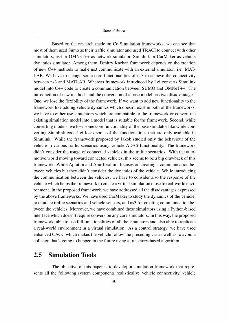
CarMaker for Simulink integrates CarMaker into the MathWorks’ modellingand simulation environment MATLAB/Simulink. The features of CarMaker are addedto the Simulink environment using an S-Function implementation and the API functionsthat are provided by MATLAB/Simulink. CarMaker for Simulink is a tightly coupledco-simulation framework resulting in a simulation environment that has both good per-formance and stability. This integration allows the use of the power and functionalityof CarMaker in the intuitive and full-featured environment of Simulink. The CarMakerGUI can be used for simulation control and parameter adjustments, as well as defin-ing manoeuvre and road configurations, IPGMovie can still be used to bring the vehiclemodel to life with realistic animation.

A new model can be built by extending the “generic” model that is availablein CarMaker for the Simulink folder. However, we can also create a model from scratchbased on our requirement with the help of CarMaker for Simulink blockset availablein Simulink library. The blockset contains useful blocks that can directly connect aSimulink model with CarMaker. These blocks can extract information from CarMakerin real-time and use them in the Simulink environment to create user-defined models.Thegeneric Simulink model of CarMaker and their blockset libraries are shown in figure 2.26

36

State of the Art

Figure 2.26. CarMaker for Simulink [29]

37

Chapter 3

Co-Simulation FrameworkArchitecture

3.1 Architecture Feasibility Study

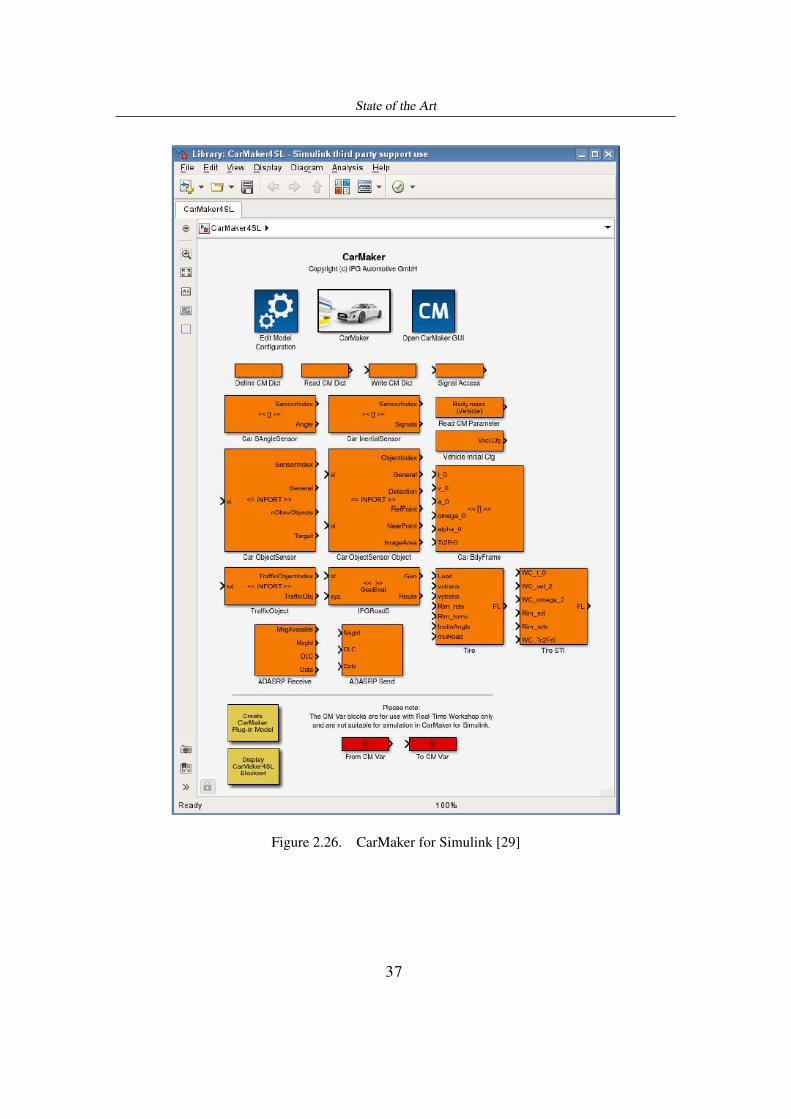
As we discussed in the previous section, the objective of this thesis is to cre-ate a co-simulation framework that represents vehicle dynamics and sensors, traffic, andcommunication. Through analytical and experimental methods, we have explored mul-tiple architectures with various simulators to fulfil the purpose of this thesis work. Wehave explained the drawbacks of the architectures that were not able to communicatewith other simulators to create a co-simulation environment.

Figure 3.1. Basic Framework Architecture

Figure 3.1 shows the base architecture of the framework. Aimsun was used tosimulate traffic vehicles (Lead Cars) and their mobility behaviours. We have used Car-Maker to study the dynamics of vehicles and emulate the vehicle sensors whereas theLTE simulator focussed on providing communication functionality to each car involved

38

Co-Simulation Framework Architecture

in the simulation. We have considered using SimuLTE (OMNeT++) and ns3 as LTEsimulators. Simulink was used to implement the control strategies which take vehicledata as inputs and define the ego car actions while considering the surrounding trafficactors. The idea of this architecture is to get traffic vehicles (lead cars) from the Aim-sun simulator and introduce them in the CarMaker environment or vice versa. By thismethod, traffic vehicles can see the ego car whereas ego car simulated in CarMaker ableto see the presence of other cars through sensors. LTE simulator can help the cars in-volved in the simulator to communicate with each other and/or infrastructure through theLTE framework. With the help of this information, Simulink would decide the ego car’smode of action i.e. accelerating/decelerating the vehicle. The simplicity of the architec-ture also becomes the major drawback of this framework. Since each of these simulatorsare written in different programming language there is no common platform to combinethem. Moreover, we have tried to establish communication between them through socketprogramming techniques. It didn’t work as expected because each simulator uses differ-ent simulation step size some are event-driven simulators while others are time-drivensimulators. Each of them runs their simulation in a different period without any syn-chronisation. To synchronise their communication between them, we needed a commonplatform that can act as a mediator between the simulators.

3.1.1 Feasibility Study 1

Figure 3.2. Framework Architecture with SUMO

We have included SUMO into the architecture as shown in figure 3.2, toact as a mediator between LTE and CarMaker through TraCI and APO library respec-tively. The idea of this architecture is to simulate the traffic vehicles in SUMO andAIMSUN through traces. With the help of TraCI, vehicles simulated in SUMO can use

39

Co-Simulation Framework Architecture

the functionalities of the LTE simulator to establish vehicular communications. Throughthe CarMaker APO library, vehicles in SUMO can be re-created in the CarMaker envi-ronment. The main drawback of this framework is Aimsun was not able to communicatewith SUMO in real-time, only traffic traces can be used in Aimsun. This behaviourended up creating a one-way communication between simulators while we were unableto create feedback loop from Aimsun to update the vehicle status back n forth. This isone of the requirements to create a complete co-simulation framework where we shouldbe able to simulate scenarios close to the real-world.

3.1.2 Feasibility Study 2

Figure 3.3. Framework Architecture with EAI

In Aimsun Next 8.4, they have introduced External Agent Interface (EAI)which can be used to exchange information with other simulators in real-time.The Frame-work Architecture with EAI is shown in figure 3.3. We tried to use this interface to over-come the drawback posed by previous architectural design. Even though, this EAI wasworking well on the Windows platform, we were unable to reproduce the same behaviourin the Ubuntu platform due to software issues. Apart from that, we were unable to createa link between the CarMaker and LTE simulator without SUMO. The main functionalityof both Aimsun and SUMO is to simulate the mobility models. Using SUMO only toestablish an interface between two simulators doesn’t do justice for the simulator. So, wehave started to explore other possibilities of creating a co-simulation framework. Withthe help of an extensive feasibility study, we were able to create a loosely coupled co-simulation framework that satisfies the thesis requirements. The system architecture and

40

Co-Simulation Framework Architecture

their functionalities are explained in the following sections of this chapter.

3.2 System Architecture

The system architecture aims at creating a loosely coupled Co-Simulationframework that combines the strength of multiple simulators to study the impact of con-nected vehicles in safety applications. It is designed as a Python-based interface thatacts as a middle-ware to enable the interoperability of multiple simulators.The finalisedsystem architecture is shown in figure 3.4

Figure 3.4. Co-Simulation Framework Architecture

The co-simulation framework composed of:

1. The ns3 module, which simulates the wireless communication net-work, including the network infrastructure and vehicles equipped withOn-Board Units (OBU);

2. The Python engine, which takes as input the information provided bythe other modules and implements the algorithms/logics for the deci-sions to be made at system/vehicle level;

3. The CarMaker module, which simulates the vehicle dynamics, the ve-hicle on-board sensors, and the vehicle traffic;

4. The MATLAB/Simulink module, which acts as an interface betweenthe Python engine and CarMaker.

41

Co-Simulation Framework Architecture

The Python engine has two main functions: (i) to connect Simulink (hence,CarMaker) with the ns3 simulator, and (ii) to host the control strategies. In more detail,CarMaker is used to model the Ego and Lead Car based on the predefined models. Withthe help of CarMaker built-in scenario builder and manoeuvre, we set our simulation ina predefined environment and monitor the movements of the Ego Car and Lead Cars.With the control strategy implemented in Python Engine, we must create an interfacebetween CarMaker and Python Engine. However, there is no direct way to integrateCarMaker with Python, so we have used CarMaker for Simulink as an interface to extractthe Vehicle Data from CarMaker environment. The data extracted from each vehicle islisted in table 3.1

Information Usage in Control Algorithm

Vehicle Position For predicting vehicle positionin next n seconds systemVelocity

HeadingLink ID For positioning the vehicle

in simulation road networkLane IDRoad ID

Steering Angle To identify cut-in/cut-out scenariosRADAR Object Detection Available only for Ego car.

To implementAdaptive Cruise Control

RADAR relative distanceRADAR relative speed

Table 3.1. Data extracted from each vehicle and their Importance

To make Simulink interact with the Python engine, we have exploited MAT-LAB commands along with MATLAB Engine API for Python. Once the vehicle data isaccessible from Python Engine, we have used the ns3 network simulator to implementV2I communications to send the Vehicle data as CAM Messages to the InfrastructureNode. After receiving the data of all vehicles involved in the simulation, infrastructurenode executes the control strategies and find the desired Ego Car acceleration. The de-sired acceleration is communicated to the ns3 Ego Car node. The Ego Car node sendsthe acceleration to the Simulink through TCP/IP connection while Simulink has beenused to update it in the CarMaker environment. The two important points to be notedas a functionality of this simulation framework are: First, the exchange of vehicle infor-mation with infrastructure node and Ego Car acceleration is designed to happen every100ms. We have set 100 ms as our simulation step, to support the fact that only 10CAM messages are allowed in 1 second; Second, as per CarMaker functionality, we can

42

Co-Simulation Framework Architecture

only update the acceleration of Ego car while parameters and manoeuvres of Lead Carsare fixed before starting of the simulation. Therefore, in this framework, we are onlycontrolling the Ego car acceleration.

As a result, with the help of Python Engine as a middle-ware, we have lever-aged all functionalities of CarMaker and ns3 to create a simulation framework that couldanalyse the impact of the connected vehicle in safety applications.

3.3 System Definition

3.3.1 CarMaker: Vehicle and Mobility Model

We have to define the vehicle model, traffic parameters and vehicle manoeu-vres before running the simulation in CarMaker. The car used by the simulation frame-work as Ego Car and Lead Car is the “DemoCar”, that is a Volkswagen Beetle. The cardynamic was maintained, except for the gearbox, which was changed from manual toautomatic. Among multiple sensors in CarMaker, we have used RADAR to detect thesurrounding objects which helps Ego Car to implement the ADAS functionalities. InCarMaker, we have added “RadarL” as an object sensor in front of the car with a cover-age distance of 150m as shown in figure 3.6. The observation area of this RADAR modelis showing in the figure 3.5.

Figure 3.5. RADAR Observation Area [30]

43

Co-Simulation Framework Architecture

Figure 3.6. CarMaker RADAR selection window

Figure 3.7. CarMaker Driver Window

44

Co-Simulation Framework Architecture

Given that the Python Engine implements the control strategies based on theinformation received through the ns3 simulator, we have to avoid the control actionsimplemented by CarMaker. Normally in CarMaker, the IPGDriver module enables thecontrol actions of a human driver such as steering, braking, gas pedal position, gearshifting, and clutch operation. In order to avoid the IPGDriver reacting to the Trafficobjects, we have unchecked the “Consider Traffic” option given by CarMaker underthe Driver section as shown in figure 3.7. By doing so,the IPGDrive just follows themanoeuvre mentioned in the test run without considering the traffic objects defined inthe TestRun.

To make the CarMaker model ready for a TestRun, we have to define Ego carmanoeuvre, Traffic Objects, and their manoeuvres along with the road topology used bythe simulation. However, these definitions are not fixed, each of them will vary basedon the simulation test scenarios. In this thesis, we have tested the framework with threedifferent test scenarios which will be explained in the next chapter.

3.3.2 Simulink: Simulation Control and Interface

As we discussed in section 2.5.2, the Simulink model can be built as an exten-sion of “generic” model provided by CarMaker. We have made changes in the genericmodel to make it interoperable with other simulators and to extract the specific dataquantiles from the CarMaker environment.

Simulink being a discrete time based simulator , it computes block methodsand states at the end of each simulation step. The simulation time step is decided bysolver: fixed or variable step depends on the simulation environment. CarMaker forSimulink works with the standard Simulink solvers. The step size of simulation in Car-Maker is 1ms. So, for every 1ms Simulink evaluates each block in the model and definetheir states. On the other hand, ns3 network simulator is a discrete event simulator whichexecutes all scheduled events independent of the time. To make them communicatewith each other, we have to pause the Simulink model execution after every predefinedtime step. We chose to pause the Simulink simulation after every 100 ms . Again, thechoice of 100 ms is justified by the fact that only ten CAM messages are allowed forevery second, that is 1 CAM for every 100 ms. We have created our own subsystem topause the simulation after every 100ms. Using simulation clock block, we constantlymonitor the simulation time and “pause” the simulation every 100 ms using assertioncommand.Figure 3.8 shows the Simulation control subsystem.

45

Co-Simulation Framework Architecture

Figure 3.8. Simulink Simulation Control Subsystem

We have used CarMaker for Simulink blocks to get the CarMaker variableslisted in table 3.1 in the Simulink environment. But Ego Car is the only fixed vehicle thatcan be available in all framework simulation scenarios while other traffic actors (LeadCars) are highly variable based on the simulation scenario. To avoid manually changingthe simulation model for each scenario, we have created a Matlab function to create thoseblocks and connect them automatically for every scenario.

To interact with other applications, Simulink suggests using TCP-IP Send/Receiveblocks. Currently, this block only supports a few datatypes like Double, integer, ASCII.Since we have to exchange vehicle information of each vehicle with different data typesto the python engine, we are forced to create multiple TCP connections between themwhich are not advisable. As a workaround, we have concatenated all the vehicle infor-mation into a matrix form using a matrix concatenate block as shown in figure 3.9. ButSimulink TCP IP doesn’t support to send data in a matrix format, so we have exploited

46

Co-Simulation Framework Architecture

MATLAB RunTimeObject functionality to exchange the information with python en-gine.

Figure 3.9. Simulink Matrix Concatenate

Figure 3.10. Simulink TCP/IP Subsystem

On the other hand, the decision made by the python engine to control the ac-celeration of the Ego car is a double value which can be received through SimulinkTCP/IP block. So, we have used TCP/IP receive block as shown in figure 3.10 to getthe desired Ego Car acceleration from the python engine. In the framework, Simulink

47

Co-Simulation Framework Architecture

TCP/IP blocks acts a client whereas Python Engine acts as a server.By this way, Pythonengine can directly communicate with Simulink in real-time without using MATLAB asa middle-ware which comparatively consumes more time to transfer the data.

3.3.3 ns3: Communication Model

ns3 being a discrete event simulator, the notion of time doesn’t work in thesame way as other simulators used in the Framework. By default, ns3 simulator advancesthe simulation time to the next scheduled event and keep on executing the scheduledevents in future without waiting. In order to integrate with other applications, ns3 has anoption to run simulations in a real-time with the help of real-time scheduler. In real-timescheduler, instead of advancing the simulation time ns3 moves it synchronously withthe machine clock. By this way, after executing an event, ns3 scheduler compares thecurrent time and next scheduled event time. If the event is scheduled in the future, ns3goes in to sleep state till the scheduled time and then executes the event. Since this isa co-simulation framework and it involves multiple simulators, we have used real-timescheduler in ns3 to schedule the events.

In this co-simulation framework, we have adopted cellular vehicle-to- Infras-tructure as our communication technology. In ns3, LTE module is implemented by theLENA simulator.LENA is an open source LTE/EPC Network Simulator that helps us todesign and evaluate the performance of LTE framework.The LENA code is merged withthe official version of ns-3.

As we know, the primary nodes of LTE module are UserEquipment(UE) andeNodeB(eNB). In this framework, we have placed eNodeB at the centre of the topologyin all scenarios. The traffic scenarios were built with the consideration of placing eNodeBat (0,0,0) position. In ns3 “ConstantPositionMobilityModel” was used to keep eNodeBat the centre of the topology for whole simulation period.

With the help of Evolved Packet Core(EPC) helper class, ns3 automaticallycreate a PGW node to handle the traffic from/to LTE radio access network. In simplewords. with the help EPC helper class , ns3 able to create end-to-end IP connectivitybetween multiple UE’s and remote hosts. We have created a remote host to act as aninfrastructure node to implement the longitudinal control algorithm. The connectionbetween PGW node and the infrastructure node was established via a point-to-point link.

In this case vehicles were considered as UserEquipment’s. The number ofUE’s varies according to the simulation scenario. In every simulation step, the positionof UE’s nodes is updated based on the vehicle position in CarMaker. The connectionbetween UE’s and remote host was established with the help of UDP sockets.

48

Co-Simulation Framework Architecture

To recreate a real-world urban environment, we have created buildings aroundeNodeB by using the ns3 Buildings module. The buildings module also implements thepropagation loss model to be used with the LTE module along with the consideration ofwall penetration losses. Based on the node’s position , buildings module decides whetherthe node is indoor or outdoor. In our case, all the nodes are considered as outdoor nodesand corresponding propagation loss model is used.

Since Python Engine plays a role of integrator between multiple simulators,all the above mentioned ns3 functionalities are scripted in Python with the help of ns3Python bindings and simulation script is integrated into the Python Engine.

3.4 Co-Simulation Interface

3.4.1 Interaction between CarMaker and Simulink

As we discussed earlier in section 2.5.2, CarMaker for Simulink helps to cre-ate a tightly coupled simulation framework between CarMaker and Simulink. In thissection, we have discussed the interaction between CarMaker and Simulink and how wewere able to exchange the values with each other.The variable exchange between Car-Maker and Simulink became possible with the help of Direct Variable Access Method.CarMaker for Simulink blockset has two blocks that is used to manipulate the variable inCarMaker environment. Those two blocks are “Read CM Dict” and “Write CM Dict”.However, these blocks can be used to get the variables that were already defined in Car-Maker data dictionary. If we want to read other values from CarMaker environment, wehave to use “Define CM Dict” to create those variables in its data dictionary.

“Read CM Dict” reads a variable in CarMaker dictionary and deliver it in theOutput port of the block in real-time. For example, if we want to know the velocity of theEgo car, we can use “Car.v” as a variable name in the block and get the current velocityas shown in figure 3.11. The name of the variable is based on the property of the vehiclewe would like to read from CarMaker, and this can be known easily from DVA sectionof CarMaker GUI. In this simulation framework, we are using RADAR object sensor todetect the traffic actors around Ego Car.Table 3.2 has the details of the variable nameused to get value from CarMaker Ego Car and lead cars where [TName] varies with thename of the traffic object.

49

Co-Simulation Framework Architecture

Figure 3.11. CarMaker Read block in Simulink

Information Ego Car Lead Car<EPre>:Sensor.Object.RadarL.relvTgt; <LPre>:Traffic.[TName]

Vehicle PositionCar.tx <LPre>.txCar.ty <LPre>.tyCar.tz <LPre>.tz

velocity Car.v <LPre>.LongVelHeading Car.Fr1.rz <LPre>.rzLink ID Car.Road.LinkObjId <LPre>.LinkObjIdLane ID Car.Road.Lane.Act.isRight <LPre>.Lane.Act.isRight

Steering Angle Driver.Steer.Ang <LPre>.SteerAngRoad ID Car.Road.sRoad <LPre>.sRoad

Radar Object Detection <EPre>.dtctNot ApplicableRadar relative distance <EPre>.NearPnt.ds_p

Radar relative speed <EPre>.NearPnt.dv_p

Table 3.2. CarMaker Variable Dictionary [30]

On the other hand,“Write CM Dict” is used to write updated value in Car-Maker data dictionary. In this framework, we are updating the Acceleration of theEgo Car in CarMaker environment based on the output of control algorithm using “Ac-celCtrl.DesiredAx” as a variable name. Since this variable is not available in CarMakerdata dictionary, we have created it using “Define CM Dict” and then update its valueusing “Write CM Dict” on every simulation step as shown in figure 3.12.

50

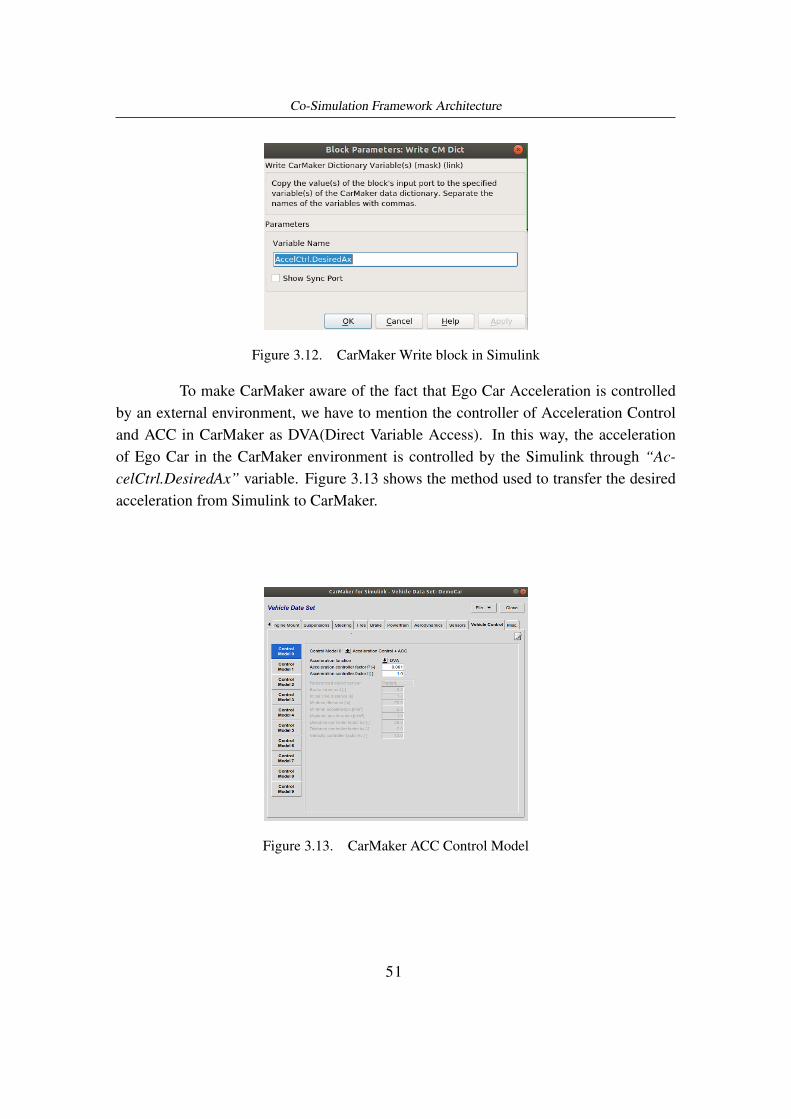
Co-Simulation Framework Architecture

Figure 3.12. CarMaker Write block in Simulink

To make CarMaker aware of the fact that Ego Car Acceleration is controlledby an external environment, we have to mention the controller of Acceleration Controland ACC in CarMaker as DVA(Direct Variable Access). In this way, the accelerationof Ego Car in the CarMaker environment is controlled by the Simulink through “Ac-celCtrl.DesiredAx” variable. Figure 3.13 shows the method used to transfer the desiredacceleration from Simulink to CarMaker.

Figure 3.13. CarMaker ACC Control Model

51

Co-Simulation Framework Architecture

3.4.2 Interaction between Simulink and MATLAB

Simulink provides an API called block run-time interface, to access the blocksdata programmatically during the simulation. By using this interface, it’s possible toaccess the run-time data from the MATLAB command line.

For accessing a Simulink block data in run-time from MATLAB, we have tocreate run-time object of that particular block. We can create a run-time object of a blockin MATLAB by using “get_param” in command line. “get_param(Object, Parameter)”return the value of the specified block. In our case , object is the Simulink block nameand parameter is “RuntimeObject”. In our case, we needed to access the blocks thatcontains the vehicle information. As discussed earlier in the Simulink Model, we haveconcatenated all the vehicle information into a Matrix form using Matrix Concatenateblock. So, we created run-time objects for every matrix concatenate block that is basedon the number of vehicles involved in the simulation. In this way, we have accessed thevehicle information from MATLAB command line in run-time.

We can also control the Simulink simulation execution from MATLAB com-mand line by using “set_param” command. “set_param(Object,ParameterName,Value)”is used to set specified value to the blocks parameter. To control the simulation, we haveto use simulation Model Name as Object, “SimulationCommand” as parameternameand we can choose one of [“start”,”pause”,”continue”,”stop”] as value. For example,set_param(“generic.mdl”,”SimulationCommand”,”pause”) is used to pause the runningsimulation.

With the help of these commands, we have manipulated the Simulink simula-tion process to synchronize with other simulators.

3.4.3 Interaction between MATLAB and Python Engine

MATLAB provides a Python package that enables Python to use MATLABas a computational engine. The MATLAB package contains MATLAB Engine API forPython and a set of MATLAB arrays that can be used as Python Variables. The engineprovides functions to call, and the array classes provide functions to create MATLAB ar-rays that can be used to send as arguments for functions. MATLAB Engine API providestwo different ways to access the MATLAB.

start_matlab - starts a new MATLAB process, and returns engine objectfor communicating with the MATLAB. We can start the MATLAB process with/withoutdesktop from Python by using start-up options. However, without-desktop(headless)option restrict us from using certain functionalities.

52

Co-Simulation Framework Architecture

connect_matlab - connects to the shared MATLAB session which is al-ready running on the local machine and returns an engine object as eng. Before us-ing connect_matlab, we have to share the running MATLAB process by executing mat-lab.engine.ShareEngine command in its command window. We can identify the sharedMATLAB process in python with the help of find_matlab. It finds all shared sessions onthe local machine and returns their names in a tuple. Therefore, we can connect to theshared MATLAB process from Python using connect_matlab (find_matlab()[desiredIndex])function.

After connecting to a MATLAB process, we can access its workspace vari-ables from Python using eng.workspace[variableName]. We can also take advantage ofall the functionalities of its command window from python with the help of eng.eval(command,nargout=) where eng represents connected MATLAB process, nargout usedto specify the number of output arguments MATLAB returned to python environment.

We have combined eng.eval function with MATLAB commands explained inthe previous section 3.4.2 to control the Simulink simulation from Python Engine.Wehave paused the Simulink simulation using following command:

eng.eval(00set_param(00generic.mdl00,00 SimulationCommand00,00 pause00)00)

With the help of following commands, we have accessed the vehicle informa-tion in Simulink from Python engine.

eng.eval(00rto = get_param(00generic/carIn f o00,00RuntimeOb ject 00),nargout = 0)

eng.eval(00rto.Out putPort(1).data00),nargout = 1)

3.5 Information Flow

In the previous section 3.4, we have discussed the interaction between the sim-ulators while in this section we have explained the simulation control and its processalong with the details about the data handled by each simulator. The simulation is pri-marily controlled by a ns3 event that is scheduled to run every 100ms. Before startingthe simulation, the Python engine initialises the simulation framework with four steps.First, it finds a shared MATLAB environment and connects to it. Second, it executesthe MATLAB function to create a list of Simulink blocks that extract vehicle informa-tion from the CarMaker environment. Third, it establishes a TCP/IP connection withSimulink, where Python Engine and Simulink acts as a server and client respectively.

53

Co-Simulation Framework Architecture

And finally, a list of ns3 nodes are created to represent the vehicles involved in the sim-ulation. Once the initialisation phase is completed and successfully create a connectionbetween all the simulators, the Python engine starts the simulation by scheduling a ns3event. We have developed a system UI as shown in figure 3.14 to simplify the above-saidsimulation execution process. All the above four steps can be performed with the clickof the initiate and run button. The initiate button identifies the number of cars that aregoing to be simulated from the CarMaker TestRun file while the Run button executes theabove steps one by one in the above-mentioned order.

Figure 3.14. System User Interface

At every simulation step, ns3 scheduled event checks the status of the Car-Maker simulation using MATLAB command through the Python engine. If the simula-tion is running, it extracts each vehicle data from Simulink through MATLAB command.In order to include real-world errors in simulations, the Python engine adds a randomnormal error to the vehicle position data extracted from CarMaker. After processing thevehicle information, ns3 schedules an event where a respective vehicle node is used tosend that information to the infrastructure node using the LTE module.

54

Co-Simulation Framework Architecture

Figure 3.15. Information Flow

Once the infrastructure node receives information from all vehicles involvedin the simulation, it executes the control strategies algorithm. The algorithm implementsenhanced CACC control which uses both Ego car RADAR signal and surrounding vehi-cle information received by infrastructure node to calculate the desired acceleration forEgo Car. The details of the control strategies are explained in section 3.6. After findingthe desired acceleration, the infrastructure node sends it to the ns3 Ego Car Node, againusing the LTE module. While Ego car Node transfer that data to Simulink using TCP/IPconnection and Simulink update it to the CarMaker environment. This flow of infor-mation concludes a simulation step that gets repeated until the completion of CarMakerTestRun. The information flow blocks along with their respective simulator are shown infigure 3.15.

3.6 Control Strategy

The main idea of the control strategy algorithm is to implement the Co-operativeAdaptive Cruise Control system to avoid any collision by adjusting the speed of Ego carbased on Radar sensor input as well as CAM messages received from the infrastructurenode. In any case, control algorithm is executed for both of inputs and minimum accel-eration between them is used as desired acceleration. The acceleration/deceleration ofEgo Car depends on the sign of the chosen acceleration as shown in table 3.3.

Acceleration ActionPositive Accelerate

0 Maintian Current VelocityNegative Brake

Table 3.3. Ego Car Action based on Acceleration sign

55

Co-Simulation Framework Architecture

As per Adaptive Cruise Control system, if no object is detected the Ego carmaintains the desired cruise speed; if any object is detected it maintains the desired dis-tance gap with the detected vehicle. In this framework, we have chosen desired time gapbetween vehicles as 0.6 seconds. The desired distance gap is calculated by multiplyingdesired time gap and current Ego car velocity.

The control algorithm works based on proportional control system with pre-defined proportional gains for RADAR detected objects and variable gains for Lead Carsdetected via CAM messages. The proportional control is a feedback control systemwhich is proportional to the difference between desired and actual value. The controlalgorithm is divided into two sections: Adaptive Cruise Control (ACC) and AutomaticEmergency Braking (AEB).

As explained in section 2.3.2, AEB activated when the collision is imminent.It depends on the Time-To-Collision (TTC) value. TTC is the measure of the amountof time until the collision occurs. It is calculated by considering relative distance andvelocity of the target vehicle with Ego Car. AEB with maximum deceleration is activatedif TTC goes below 1 second.

Acceleration =−2.6m/s2,∀1 ≤ T TC ≤ 2.4

Acceleration =−9.6m/s2,∀T TC < 1

ACC uses relative distance and velocity of the target vehicle, desired distance,and speed set by Ego car as input to calculate desired acceleration. The proportionalgains used in ACC are kv1, kv2, kd , kdd . The Lead Car relative velocity with Ego Car uses00k00v1 and the difference between the relative distance and the user defined desired distanceuses 00k00d as their proportional gain. In any case, Ego car velocity is not supposed to behigher than the desired velocity set by the user, so ACC calculates the difference betweenthe desired velocity and current Ego car velocity with 00k00v2 as their proportional gain. Thesign of their difference decides whether Ego car has to accelerate or decelerate. If targetvehicle velocity is higher than the Ego car but the distance between them is less than thedesired distance, Ego can decelerate with lower gain compared to 00k00d . Therefore, wehave used 00k00dd as a proportional gain which is considerably less than 00k00d . Figure 3.16shows the ACC control scheme along with the importance of proportional gains [27].

However, the acceleration/deceleration rate is restricted to certain limit to en-sure the comfort, safety of the passengers. The gains and acceleration/deceleration limitsof ACC are mentioned in the table 3.4.

56

Co-Simulation Framework Architecture

Figure 3.16. ACC Control Scheme [27]

Specifications Value LimitsMax deceleration (ACC) [m/s2] -2.45Max deceleration (AEB) [m/s2] -9.6

Max acceleration [m/s2] 1kd 0.07kdd 0.01kv1 0.45kv2 0.3

Table 3.4. ACC Gain and Acceleration Limits [27]

The control algorithm is executed with the above-mentioned gains for radardetected objects. However, for Lead Cars that do not fall under the range of radar, we usea trajectory-based control system to predict the collisions. For every vehicle involved inthe simulation, we predict the vehicle positions for the next 10 seconds with 0.1 secondsas a difference between two predicted time instances. To predict the positions, we areusing current position, heading direction and velocity from CAM messages. With thehelp of LaneID, RoadID, LinkID information from CAM message, we are finding theLead Cars that are in the collision course with Ego car in the next 10 seconds. Sincea trajectory-based system can only detect the collisions that occurs in the straight pathbased on the current heading direction, we tend to miss the presence of vehicles in thecorners. By combining road network information’s like LaneID, RoadID and LinkIDwith the positions, we are able to detect the presence of Lead Cars in the corners.

57

Co-Simulation Framework Architecture

Figure 3.17. Distances Representation in Control Algorithm

After defining the position of the cars for next 10 seconds, we are calculatingthe distance between Lead Car and Ego car as shown in figure 3.18. If the calculateddistance (Dp) is below the safe distance (Ds) at any point in next 10 seconds , we executethe control algorithm to find the desired acceleration. The safe distance is calculatedbased on the specifications mentioned by ACI (Italian Automotive Club)[28]. The trendof safety distance is shown in figure 3.18.

Figure 3.18. ACI Safety Distance [27]

However, we can’t execute the control algorithm with normal gains mentionedin the above table because with the current distance(Dc) between Ego car and the vehiclein question normal gains doesn’t have impact in defining the acceleration. To makethe control algorithm react to the collision that might occur in the future, we have usedthe variable gains. Among four proportional gains, 00k00v1 and 00k00d plays major role in

58

Co-Simulation Framework Architecture

calculating the desired acceleration. Since, we are predicting for 10 seconds with 0.1 asa time difference, We have created 100 data points between 0 and 0.45 in case of 00k00v1and between 0 and 0.07 for 00k00d that follows the pattern shown in the figure 3.19.

Figure 3.19. Trend of Variable Proportional Gains

Among the 100 data points, the control algorithm chooses the proportional gainbased on the index of the minimum predicted distance between Ego Car and Lead Car.With those gain values, control strategy executes the algorithm with Lead vehicle currentvelocity, distance and Ego car velocity as input to identify the desired acceleration.

Currently, we have two accelerations; one from RADAR based data and an-other one from Lead Cars that doesn’t fall under the RADAR range. The Control algo-rithm choose the one with minimum acceleration as the Ego Car desired acceleration forthe next simulation step. The flow-chart of the entire control algorithm is illustrated infigure 3.20.

59

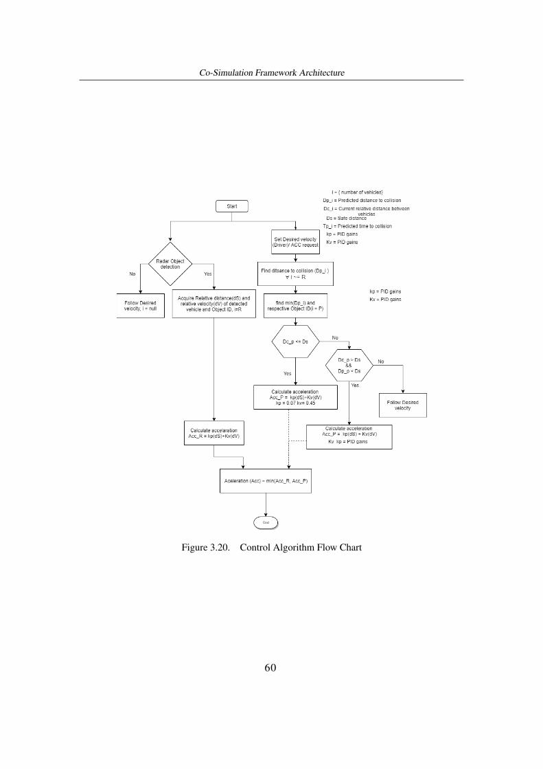
Co-Simulation Framework Architecture

Figure 3.20. Control Algorithm Flow Chart

60

Chapter 4

Simulation Scenarios andResults

4.1 Simulation Scenarios

The main goal of this framework is to study the impact of the connected vehi-cles in comfort and safety-related applications. In order to attain this goal, we have testedthe framework with a set of scenarios that can occur in the real-world. These tests areperformed to evaluate the performance of the control strategies using collision avoidanceas one of the key performance indicators. The parameters used by the control algorithmare described in table 3.1, which are extracted from CarMaker and communicated to theinfrastructure through the ns3 simulator. The default time headway between Ego Car andLead Car is fixed at 0.6 seconds and the desired cruise speed is varied between 22m/s and16 m/s based on the simulation scenario. Furthermore, the vehicle acceleration is limitedto 1m/s2 while the maximum deceleration (in case of AEB) is capped at -9.6m/s2 . Thelimits are listed are in table 3.4. The topology of the road varies based on the simulationscenario.

We have tested the framework for three different scenarios. They are:

1. Vehicles crossing in a T-Junction

2. Preceding vehicle Cut-out from the lane

3. Slower/Stationery vehicle in the Corner

61

Simulation Scenarios and Results

In order to point out the situations where vehicle sensors are not enough to mitigatethe collisions, we have simulated these three scenarios for two different modes.

• Vehicles with sensors only

• Vehicles with Sensors and OBU (Connected Vehicles)

Furthermore, in the case of connected vehicles, we have executed the controlalgorithm for different forecasting time instances(5, 7, 10 seconds) using a trajectory-based prediction model.

4.1.1 Scenario-1: Vehicles crossing in a T-Junction

In this scenario, we are using two vehicles(Ego car and a Lead Car) whichare going to meet at a T-junction. The vehicles and their manoeuvres are pre-defined inCarMaker TestRun. The road topology also created in CarMaker using Scenario Editor.The Ego car is travelling in a constant velocity of 80kmph in a straight route, mentionedas Route 1 in figure 4.1.The lead car is travelling at a lower speed while approachingthe T-junction and after crossing the T-junction Lead Car accelerate for 10 seconds withacceleration rate as 1 m/s2 as shown in figure 4.2. The route of Lead Car is marked asRoute 2 in figure 4.1. The scenario is created in a way that the lead car falls under theblind spot of the Ego car RADAR while crossing the T-junction. The Ego Car RADARrange is shown in figure 3.6. With the Lead Car being blind-sided, Ego Car tends tomaintain the desired cruise speed. We have analysed the reaction of Ego Car when itdetects the presence of Lead Car in both the modes.

Figure 4.1. CarMaker Scenario Editor

62

Simulation Scenarios and Results

Figure 4.2. Lead Car Manoeuvres

4.1.2 Scenario-2: Preceding vehicle Cut-out from the lane

In the second scenario, we are simulating a cut-out scenario where a Lead Caris changing a lane at a last minute to avoid a collision with another Lead Car in the samelane.Figure 4.3 shows the pictorial representation of this Scenario. In this case, we areusing 3 vehicles (Ego car and two Lead cars) in a straight road with two lanes. The Egocar is following a Lead car which is travelling at 80kmph while a Lead Car in front of itis travelling at a speed of 80kmph. Since, Ego car desired speed is 80kmph, it maintainsa time-headway of 0.6 seconds with the preceding Lead car. Suddenly the latter changesthe lanes to avoid the slower vehicle in front of it,figure 4.4 shows the manoeuvre definedfor the LeadCar in CarMaker to avoid the collision. The Ego car radar has less time tochange its focus to new target and react accordingly to avoid the collision at higher speed.We have analysed the use of CAM messages in this scenario to identify the presence ofslow moving vehicle beforehand and react to it promptly.

63

Simulation Scenarios and Results

Figure 4.3. Pictorial Representation of Cut-Out Scenario

Figure 4.4. Lead Car Cut-Out Manoeuvre in CarMaker

4.1.3 Scenario-3: Slower/Stationary Vehicle in the Corner

In this scenario, we have tested the limitation of RADAR to detect the presenceof a vehicles in a corner. Figure 4.5 shows the road topology used for this simulationscenario. To make the scenario more realistic we have added buildings near the cornerwhich could possibly reduce the visibility of the driver. For this simulation, we haveused two cars (Ego car and Lead car), where both the vehicles are approaching a corner.The Ego car and Lead car are travelling at 60 kmph and 45 kmph respectively, with aconsiderably longer distance between them. The desired cruise speed of Ego Car is 60kmph, so it maintains the current velocity along with the desired time headway. Whileapproaching the corner, Lead car broke down due to some mechanical malfunction andcame to a stop. Figure 4.6 shows the Lead Car manoeuvre definition in CarMaker. Giventhat Ego car radar won’t be able to see the static vehicle at the corner, it continues to travel

64

Simulation Scenarios and Results

at higher relative speed. We have analysed the different courses of action performed bythe Ego Car to avoid the collision in the two modes.

Figure 4.5. Road Topology of Scenario3

Figure 4.6. Lead Car Manoeuvre in CarMaker

65

Simulation Scenarios and Results

4.2 Results

As discussed earlier, we have simulated all the scenarios for two modes i.e withand without OBU(connected vehicles). In a case of the connected vehicles mode, Ego carshould be able to mitigate the collision without activating Automatic Emergency Braking(AEB) mode because the system constantly monitors the movements of the vehicle. Thecontrol algorithm uses 10 seconds as its default prediction time frame.

4.2.1 Scenario 1

The goal of this scenario is to identify the potential collision occurrence in theupcoming T-Junction and change the Ego Car velocity to avoid the collision by acceler-ating/decelerating the vehicle.

Figure 4.7. Scenario1: Ego Car Acceleration and Velocity variation based onRADAR and CAM Messages

The figure 4.7 show the Acceleration chosen by the control strategy algorithmby considering RADAR and CAM messages as input. It has three sub-plots. The Ac-celeration sub-plot shows the acceleration output based on RADAR and CAM messagesas well as the acceleration used by Ego Car among them. The ACC selection sub-plotindicates whether the control algorithm used ACC or CACC controller to define the de-sired Ego Car Acceleration. The Velocity sub-plot shows the velocity of the vehicle

66

Simulation Scenarios and Results

involved in the simulation, where T0 indicates the Lead Car. We can see from the accel-eration sub-plot, RADAR didn’t have any vehicle on its range, so it keeps maintainingthe desired cruise speed of the Ego Car as shown in velocity sub-plot. With the helpof CAM messages, the control algorithm identifies the presence of other vehicles in thenetwork and it predicted that the slow-moving vehicle is in the collision course with theEgo Car. Once the distance between Ego Car and slow-moving vehicle comes below thesafe distance, the control algorithm calculates the desired acceleration value to avoid thecollision and communicated it to Ego Car. Since we are foreseeing the collision that canpotentially occur in the future, Ego Car reduces the velocity gradually as happened in ve-locity sub-plot of the figure 4.7. From Acceleration sub-plot of the figure 4.7, we can alsonotice that Radar-based acceleration is increased to compensate the velocity reduction.The reason behind this behaviour is because there is no vehicle in the RADAR rangeof the Ego car, so it tries to maintain the desired cruise speed. Once the vehicle fallsunder the RADAR range, the system also switches its primary focus from Predicted toRADAR based Acceleration as shown in selection sub-plot of the figure 4.7. This can beconfirmed from the second sub-plot that shows the switch between predicted to RADARbased acceleration mode. As mentioned in figure 4.2, after crossing T-junction, the LeadCar accelerates to 60 km/h. we can see that the Ego Car also accelerates gradually tomaintain the desired distance gap between Ego and Lead Car. The rate of change of EgoCar acceleration is smooth without any abrupt deceleration/acceleration which ensurespassenger comfort and safety.

The figure 4.8 shows the simulation with and without OBU. ACC indicatesRADAR is the sole source of data for Ego car to decide the acceleration while CACCindicates the usage of CAM messages to calculate the acceleration. In this scenario, LeadCar enter in the RADAR range at the last moment, so the Ego Car activates the pre-brake(-2.6 m/s2)in AEB mode for a brief time. Given that, the reduction in velocity is notenough to avoid imminent collision, it uses full brake force of -9.6 m/s2 to avoid thecollision. We can notice the steep reduction of velocity in the velocity sub-plot of figure4.8. On the other hand, with the help of CAM messages, Ego Car detects the collisionearlier and applies the brake gradually. This can be confirmed by the smooth reductionof velocity in velocity sub-plot of figure 4.8.

The figure 4.9 shows Ego Car Acceleration trend based on different forecastingperiods ( 10,7,5 seconds). For this scenario, the prediction period of 7 seconds performbetter than the others. With forecasting time as 10 seconds, the acceleration is smooth atthe initial phase, however it is not sufficient to keep the safe distance between the vehi-cles. So, at the later stage it chooses higher deceleration value compared to 7 seconds.

67

Simulation Scenarios and Results

Figure 4.8. Scenario1: ACC vs CACC Comparision

Figure 4.9. Scenario1: Acceleration Variation for different Prediction Time Instances

The plots presented in scenario 2 and scenario 3 follows the same pattern asof scenario 1. To reduce the repetition, we have explained only the differences in thefollowing two scenarios.

68

Simulation Scenarios and Results

4.2.2 Scenario 2

The goal of this scenario is to detect the presence of a slower vehicle in thesame lane as of Ego Car and use CACC to maintain the desired time head-way betweenEgo Car and Lead Car.

In this scenario, we have 3 cars moving in the same lane. In the velocity sub-plot of 4.10 T0 and T1 represents Lead Car(1) and Lead Car(2) respectively. As shownin the velocity sub-plot of figure 4.10 the Lead car(1) which is in front of Ego Car is trav-elling at the desired cruise speed of Ego Car. Therefore, Ego Car maintains the desireddistance gap with zero acceleration as shown in Acceleration plot of 4.10. However, oncethe control algorithm detects the presence of a slower vehicle in the same lane travellingin the same direction, Ego Car decelerates to maintain the desired time headway withthe Lead Car(2) which is in front of the Lead Car(1). As expected, RADAR based ac-celeration tends to increase to maintain the cruise speed which is based on Lead Car(1)velocity. Once the Lead Car(1) realises the presence of Lead Car(2), it moves to the ad-jacent lane to avoid the collision. This abrupt action of Lead Car(1) brought Lead Car(2)in the RADAR range of the Ego Car. After the cut-out, Ego Car chose RADAR basedacceleration to maintain the desired distance while Prediction based Acceleration choseto accelerate by considering the Lead Car(1). As per the design, the control algorithmchooses the minimum acceleration between Prediction and RADAR as the desired ac-celeration of Ego Car. The trend of ACC and CACC comparison figure 4.11 is similar toscenario 1. However, since the Lead Car(1) changes the lane at the very last moment, theEgo Car reaction time is lesser than scenario 1. We can notice that AEB pre-brake acti-vation period is considerably less than the Scenario 1 because the deceleration providedby pre-brake is not sufficient to stop the vehicle moving at 80km/h. When TTC wentbelow 1 second, Ego car activates emergency brake with deceleration value of -9.6m/s2

to reduce the impact of the collision. This can be also verified by the steep reductionof Ego Car velocity in the velocity sub-plot of the figure 4.11. The prediction time in-stances figure 4.12 shows that foreseeing the collision before 10 seconds perform betterthan the others. The acceleration trend of other time instances indicates steep reductionin the acceleration while the 10-second prediction instance shows a gradual reduction inthe acceleration.

69

Simulation Scenarios and Results

Figure 4.10. Scenario2: Ego Car Acceleration and Velocity variation based onRADAR and CAM Messages

Figure 4.11. Scenario2: ACC vs CACC Comparision

70

Simulation Scenarios and Results

Figure 4.12. Scenario2: Acceleration Variation for different Prediction Time Instances

4.2.3 Scenario 3

This scenario aims to identify the stationary vehicle in the corner of a road withthe help of CAM messages and apply the control algorithm to stop the Ego Car.

In this scenario, the Ego Car cruise speed is set at 60km/h while the lead caris travelling at 45km/h. As we can see from the acceleration sub-plot of the figure 4.13,Ego Car acceleration didn’t change with the reduction of the Lead Car Velocity(T0) asshown in velocity sub-plot of 4.13. This is because the relative speed between them isvery low and the relative distance between them is very high. With the variable propor-tional gains trend shown in the figure 3.19, the control algorithm chooses the best gainto gradually reduce the acceleration. From 4.14 figure, we can see a lot of variations inACC acceleration compared to other scenarios because Ego car is reducing its velocity totake a turn around the corner. Once the Ego Car turned in the corner, RADAR identifiesthe presence of a stationary vehicle and activate AEB with full force to avoid the colli-sion. While the velocity plot of CACC shows gradual reduction in velocity as expected.The prediction time instance figure 4.15 shows the acceleration of Ego Car varies alotbefore getting stable. We can see that the Ego Car performs better with 10 seconds asthe prediction time while other time instances activates AEB pre-brake to avoid the col-lision.This indicates prediction time frame of 7 or 5 seconds is not sufficient to maintainthe TTC above 2.4 seconds, which concerns the safety of the passenger.

71

Simulation Scenarios and Results

Figure 4.13. Scenario3: Ego Car Acceleration and Velocity variation based onRADAR and CAM Messages

Figure 4.14. Scenario3: ACC vs CACC Comparision

72

Simulation Scenarios and Results

Figure 4.15. Scenario3: Acceleration Variation for different Prediction Time Instances

73

Simulation Scenarios and Results

4.2.4 General Discussion

Scenarios Quantity No Prediction(without OBU)

Prediction (with OBU)10 seconds 7 seconds 5 seconds

Scenario 1

MinimumVelocity (km/h) 27.7593 39.5807 40.4 38.6741

MinimumAcceleration (m/s2) -9.5 -1.7953 -1.5969 -2.0411

AccelerationStandardDeviation

1.6733 0.7319 0.7078 0.7858

VehicleDetectionDistance (m)

30.2753 203.5856 184.929 130.322

Scenario 2

MinimumVelocity (km/h) 24.69 29.0229 28.9579 28.8009

MinimumAcceleration (m/s2) -9.5 -1.2755 -1.6956 -2.1896

AccelerationStandardDeviation

1.9694 0.4452 0.5465 0.55

VehicleDetectionDistance (m)

20.1614 142.341 122.9626 99.9416

Scenario 3

MinimumVelocity (km/h) 0 0 0 0

MinimumAcceleration (m/s2) -9.6 -2.2965 -2.6 -2.6

AccelerationStandardDeviation

1.636 0.7443 0.8399 1.0187

VehicleDetectionDistance (m)

15.275 88.555 81.9081 70.6466

Table 4.1. Comparison of basic quantities between with and without OBU modes

Ultimately, we expected the system to avoid all potential collisions that mightoccur in the future with the help of CAM messages. We have also hoped for gradualacceleration/deceleration of the vehicle to provide a safe and comfortable journey. Theseexpectations are fulfilled by the fact that in the case of OBU (connected vehicles) mode,

74

Simulation Scenarios and Results

we were able to predict the collision in the future and implemented necessary actionsto avoid the same. From the table 4.1, we can also notice that Ego Car didn’t activatethe AEB mode in all three scenarios to avoid the collision while in No Prediction mode,the Ego Car activates AEB with full force for all the three scenarios to avoid/reduce theimpact of the collision. The minimum acceleration chosen by Ego Car in the defaultmode is -2.2965 for scenario3, where braking in the corner also played a major role inthe deceleration. The main factor of the ACC/CACC algorithm is the detection distanceand velocity, which directly relates to the reaction time of the vehicle. We can see fromthe table 4.1 that the difference in vehicle detection distance between No Prediction anddefault Prediction mode is very high. The minimum detection distance for predictionmode is 88.55m whereas for no prediction mode 15.275m. This directly reflects in theacceleration behaviour of the Ego Car. The mean standard deviation of predicted modeis 0.6404 while for no prediction is 1.7595 which shows the major variation in the EgoCar acceleration for no prediction mode. This rapid deceleration behaviour of the vehi-cle questions the comfort and safety of the passengers. Based on the discussions in theprevious section 4.2, we can say that the CACC system can identify the suitable gainsto ensure the gradual acceleration/ deceleration of the vehicle. On the other hand, if wecompare the different prediction time instances, two out of three scenarios show predict-ing the collision before 10 seconds helps us to reach our expectations. But in the Scenario1, prediction time frame of 7 seconds gave us better results compared to others. This canbe verified from velocity, acceleration, acceleration standard deviation quantities men-tioned in the table 4.1. However, in Scenario 3 it forces the vehicle to activate AEB toavoid the collision. We are developing a vehicle safety-related application where the pre-diction of the future time instance means finding a potentially critical situation and reactto it beforehand. With less forecasting period,we are risking the safety of the passengersby providing less reaction time to the vehicle . From the table 4.1 and plots presented inprevious section 4.2, we can safely conclude that CACC with the prediction time frameof 10 seconds is the most suitable parameter selection for the presented scenarios.

75

Chapter 5

Conclusion

In this thesis, we have created a co-simulation framework that focuses on in-tegrating the functionalities of multiple simulators such as CarMaker, ns3, Simulink tostudy the impact of connected vehicles in safety-related applications. We have used Car-Maker to analyse the dynamics of vehicles, emulate the on-board sensors activities andto create mobility scenarios. ns3 simulator is used to simulate the behaviour of vehicularcommunications. We have adopted the LTE based V2I system as our communicationmodel where we have exploited ns3 LENA implementation to model the LTE frame-work. To combine the strengths of these two simulators, we have used Simulink andPython Engine as our interface. Simulink along with MATLAB is used to exchange in-formation between Python Engine and CarMaker whereas ns3 Python bindings are usedto perform the ns3 simulation in Python environment. The Python Engine controls theexecution of all the simulators. Once a framework is established to combine these simu-lators, we have developed a control strategy to evaluate the performance of our system.The control strategy uses CAM message that contains the information of all vehicles inthe network to predict any possible collision incident in the future. We have applied atrajectory-based collision detection system to calculate the position of the vehicles invarious prediction time frames (10,7, 5 seconds). With the foreseen vehicle positions,we were able to identify the vehicles that are in the collision course with the Ego Car. Toavoid the collision, the CACC algorithm is used to calculate the desired acceleration ofthe Ego Car. Through the Simulink interface, we have communicated this desired accel-eration data to the CarMaker environment. The control algorithm also considers the EgoCar RADAR information to calculate the desired acceleration. After the creation of thecontrol strategy, we have performed multiple experiments with various traffic scenarioswhere the mobility pattern of the Lead Cars are defined in a way to test the effect of ve-hicular communications in safety-related applications. The tested scenarios are Ego and

76

Conclusion

Lead Car crossing in a T-junction, Lead Car which cut-out at a high speed exposing EgoCar to a slow-moving vehicle, the stationary Lead car at the corner. The importance ofthe connected vehicles in traffic efficiency and safety is magnified by looking at the re-sults section. The Ego Car which is equipped with OBU was able to predict the collisionand avoid them with gradual acceleration/deceleration whereas Ego Car that dependsonly on-board sensors for avoiding collision ended up activating AEB to avoid/reducethe impact of the collision.

The main achievements of this thesis work are: developing a co-simulationframework that can combine multiple simulators without compromising their function-alities; developing a control strategy that can exploit both ACC and CACC controllersto ensure the passenger comfort and safety; analysing the importance of the connectedvehicles in vehicular safety applications.

In the future, we will do extensive experiments that include multiple scenarioswith complex traffic conditions where lateral movements are also performed to avoida collision. The flexibility of the framework allows us to replace the CarMaker mod-ule with Simulink and Simulation of Urban Mobility (SUMO). Simulink can be used tomodel the vehicle dynamics, onboard sensors while the SUMO can represent the vehicletraffic. By using Simulink and SUMO, we can control all the cars involved in the sim-ulation which is not possible in CarMaker. We will exploit the hybrid communicationmodels where V2V with WAVE standard can be used to support platooning related ap-plications while V2I with LTE standard can be used to forecast the collisions that mightoccur in the future.

77

Bibliography

[1] United Nations Population Fund, https://www.unfpa.org/sites/default/files/pub-pdf/695_filename_sowp2007_eng.pdf.

[2] Association for Safe International Road Travel, https://www.asirt.org/safe-travel/road-safety-facts

[3] The European Transport Safety Council, https://etsc.eu/euroadsafetydata/[4] TomTom Traffic Index, https://www.tomtom.com/en_gb/traffic-index/[5] INRIX Traffic Scorecard, https://inrix.com/press-releases/

2019-traffic-scorecard-uk[6] Y. L. Tseng. LTE-Advanced Enhancement for Vehicular Communication. IEEE

Wireless Communications, Dec 2015.[7] Fabio Arena and Giovanni Pa (2019).An Overview of Vehicular Communications,

Future Internet Journal[8] G. Araniti, C. Campolo, M. Condoluci, A. Iera, A. Molinaro, LTE for Vehicular

Networking: A Survey. IEEE Communications Magazine,May 2013[9] J. Schlienz and A. Roessler. Device to device communication in lte. Technical Re-

port, ROHDE and SCHWARZ, 2016[10] 3rd Generation Partnership Project. 3GPP technical specification group radio access

network study on lte-based v2x services (release 14). Technical Report TR 36.885V14.0.0, 3GPP, 2016.

[11] Alexandre K. Ligo, Jon M. Peha, João Barros,Throughput and Cost-Effectivenessof Vehicular Mesh Networks for Internet Access, September 2016

[12] Daniel Jiang, Luca Delgrossi,IEEE 802.11p: Towards an International Standard forWireless Access in Vehicular Environments, May 2008

[13] Mila Romana Cécile Tabacoff, Cellular and DSRC approaches for vehicular traf-fic safety, Politecnico Di Torino Thesis https://webthesis.biblio.polito.it/8233/, 2018

[14] José Santaa, Fernando Pereñígueza, Antonio Moragóna, Antonio F. Skarmeta, Ex-perimental Evaluation of CAM and DENM Messaging Services in Vehicular Com-munications. Transportation Research Part C Emerging Technologies, September2014

[15] Ondrej Burkacky, Johannes Deichmann, Georg Doll, and Christian Knochenhauer(2018)."Rethinking car software and electronics architecture". mckinsey.com article

78

Bibliography

[16] Alice Matthews(2017) "What is driving the automotive LiDAR and RADAR mar-ket?".electronicspecifier.com article

[17] National Highway Traffic Safety Administration, Critical Reasons for Crashes In-vestigated in the National Motor Vehicle Crash Causation Survey, March 2018

[18] Anders Cioran (2015). “System Integration Testing of Advanced Driver AssistanceSystems”. KTH royal institute of technology school of electrical engineering, Swe-den.

[19] Intelligent transport systems — Cooperative adaptive cruise control systems(CACC) — Performance requirements and test procedures,ISO 20035:2019. https://www.iso.org/obp/ui/#iso:std:iso:20035:ed-1:v1:en

[20] Dmitry Kachan (2010) Integration of ns3 with MATLAB\Simulink.Lulea Univer-sity of Technology,Sweden

[21] Jakob Kaths,Sabine Krause (2017) Integrated simulation of microscopic traffic flowand vehicle dynamics.Conference:IPG Apply and InnovateAt,Karlsruhe

[22] Chenxi Lei, Emiel Martijn van Eenennaam, Wouter Klein Wolterink, Jeroen Ploeg,Georgios Karagiannis and Geert Heijenk. Evaluation of CACC string stability usingSUMO, Simulink, and OMNeT++. EURASIP Journal on Wireless Communicationsand Networking 2012, 2012:116

[23] Amr Ibrahim, Chetan Belagal Math, Dip Goswami, Twan Basten, Hong Li. Co-simulation Framework for Control, Communication and Traffic for Vehicle Pla-toons.21st Euromicro Conference on Digital System Design (DSD),2018 .

[24] Apratim Choudhury, Tomasz Maszczyk, Muhammad Tayyab Asif, Nikola Mitro-vic,Chetan B. Math, Hong Li and Justin Dauwels (2016).An integrated V2X simu-lator with applications in vehicle platooning.IEEE 19th International Conference onIntelligent Transportation Systems.

[25] Network Simulator, ns3 https://www.nsnam.org[26] Network Simulator,ns3 Python bindings. https://www.nsnam.org/wiki/

Python_bindings[27] Alberto Arcidiacono, ADAS virtual validation: ACC and AEB case study with IPG

CarMaker, Politecnico Di Torino Thesis https://webthesis.biblio.polito.it/8276, 2018

[28] ACI (Italian Automobile Club) (1992). “Art. 149. of New road codex - safety dis-tance between vehicles. Decree of the President of the Republic 16 December 1992,n.495.

[29] IPG CarMaker (2019). “Programmer’s Guide Version 8.0”. Bannwaldallee60,76185 Karlsruhe, ipg-automotive.com

[30] IPG CarMaker (2019). “Reference Manual – Version 8.0”. Bannwaldallee 60,76185Karlsruhe, ipg-automotive.com.

79