POLITECNICO DI TORINO DEPARTMENT OF MANAGEMENT AND ...

POLITECNICO DI TORINO

DEPARTMENT OF MANAGEMENT AND PRODUCTION ENGINEERING

DIGEP

VINÍCIUS DE FREITAS PACHECO

Benchmarking in additive manufacturing systems with photopolymers through part

quality analysis

TURIN

2020

VINÍCIUS DE FREITAS PACHECO

Benchmarking in additive manufacturing systems with photopolymers through part

quality analysis

Graduation work presented to Politecnico di Torino in order to achieve the title of Master of Science (Laurea Magistrale) in Mechanical Engineering.

Supervisors: Prof. Paolo Minetola Prof. Flaviana Calignano

TURIN

2020

This work is dedicated to the Italian people,

who welcomed me into their home and taught me so

much over the years that I was in their country. It is

also dedicated to my parents, with admiration,

gratitude, and affection for the support they have

always given me on my journey.

ACKNOWLEDGEMENTS

A grateful acknowledgement to Professor Paolo Minetola for welcoming me in the

elaboration of the thesis, and providing all the support and equipment necessary for the research.

I am also greatly thankful to Giovanni Marchiandi from Politecnico di Torino’s RMLAB, for

supporting the experimental development of the thesis and helping me in the most diverse

obstacles.

To Politecnico di Torino and the Department of Management and Production

Engineering (DIGEP), I am grateful for the opportunity of taking the Mechanical Engineering

Master’s of Science course, in a Double Degree partnership with the University of São Paulo.

ABSTRACT

PACHECO, Vinícius de Freitas. Benchmarking in additive manufacturing systems with

photopolymers through part quality analysis. 2020. Thesis (Master of Science degree in

Mechanical Engineering) – Politecnico di Torino, Turin, 2020.

Additive manufacturing, or 3D printing, has attained a widespread popularity as machines and

equipment necessary for fabrication have become more accessible. These manufacturing

processes, however, have each their own limitations and capabilities. For instance, every

machine to its own process will be able to fabricate a similar product, with different errors and

accuracies. As a result, it is important that a machine’s capabilities are known prior to utilization,

so that the automated operations of the additive manufacturing (AM) system are capable of

producing a part with the desired dimensions and geometries. In this study, a benchmarking

analysis is conducted among three different AM systems for processes involving

photopolymers. Accuracy is evaluated in terms of ISO IT grades and standards of geometric

dimensioning and tolerancing, in order to compare machines that produced the same reference

artifact in stereolithography (SLA), digital light processing (DLP) and PolyJet.

Keywords: 3D printing; SLA; DLP; PolyJet; ISO IT grades; Additive manufacturing.

LIST OF FIGURES

Figure 1 – Timeline with a select amount of additive manufacturing processes, based on

patenting dates. ......................................................................................................................... 17

Figure 2 – User part CAD model.............................................................................................. 21

Figure 3 – Mahesh part CAD model. ....................................................................................... 21

Figure 4 – Moylan et. al CAD model (modified). .................................................................... 23

Figure 5 – Cruz Sanchez et al. CAD Model with identification ID’s. ..................................... 24

Figure 6 – Minetola et al. CAD Model with identifications. .................................................... 25

Figure 7 – Juster & Childs CAD Model. .................................................................................. 25

Figure 8 - Fahad & Hopkinson CAD Model. ........................................................................... 26

Figure 9 - Sharebot Antares SLA printer.................................................................................. 28

Figure 10 – Sharebot Rover DLP printer.................................................................................. 29

Figure 11 – Stratasys Objet30 Prime PolyJet printer. .............................................................. 30

Figure 12 – Generic Coordinate Measuring Machine Representation. .................................... 32

Figure 13 – Poli Light Man CMM Machine. ........................................................................... 33

Figure 14 – Stylus dimensions for terminology. ...................................................................... 34

Figure 15 – Effective working length of a measuring probe. ................................................... 35

Figure 16 – Renishaw 1mm probing tool at Politecnico di Torino. ......................................... 35

Figure 17 - Staircase effect in layer manufacturing using variable layer thickness. ................ 40

Figure 18 – Proposed artifact part. ........................................................................................... 41

Figure 19 – Comparison between 45° and 90° overhangs and supporting necessities. ........... 42

Figure 20 – Generic arrangement of the part with regards to the build tray. ........................... 42

Figure 21 – Probe Clearance Zone. .......................................................................................... 44

Figure 22 – Visual representation of the artifact highlighting the feature family A. ............... 46

Figure 23 – Visual representation of the artifact highlighting the feature family B. ............... 46

Figure 24 – Visual representation of the artifact highlighting the feature family C. ............... 47

Figure 25 – Visual representation of the artifact highlighting the feature family D. ............... 47

Figure 26 – Visual representation of the artifact highlighting the feature family E. ................ 48

Figure 27 – Visual representation of the artifact highlighting the feature family F. ................ 48

Figure 28 – Visual representation of the artifact highlighting the feature family G. ............... 49

Figure 29 – Visual representation of the artifact highlighting the feature family H. ............... 49

Figure 30 – Sectioned representations of the staircase feature, viewed from the top of the part.

.................................................................................................................................................. 50

Figure 31 – Visual representation of the artifact highlighting the feature family I. ................. 50

Figure 32 – Visual representation of the artifact highlighting the feature family J. ................ 51

Figure 33 – Sectioned view of the rectangular boss feature, seen from atop of the part.......... 51

Figure 34 – Visual representation of the artifact highlighting the feature family K. ............... 52

Figure 35 – Visual representation of the artifact highlighting the feature family L. ................ 52

Figure 36 – Visual representation of the artifact highlighting the feature family M. .............. 53

Figure 37 – Visual representation of the features that compose families N and O. ................ 54

Figure 38 – Visual representation of the artifact highlighting the planes selected for family P.

.................................................................................................................................................. 54

Figure 39 – Support structure preparation in Sharebot’s company-made software for the DLP

Sharebot Rover. ........................................................................................................................ 56

Figure 40 – Sharebot Antares build platform when sanitized (left) and isopropyl used (left). 56

Figure 41 – Printing initialization of the Sharebot Rover for the DLP replica. ....................... 57

Figure 42 – DLP test part after printing completion. ............................................................... 58

Figure 43 – Removal of the DLP part from the printing platform. .......................................... 58

Figure 44 – Sharebot Antares open for initialization. .............................................................. 59

Figure 45 – Close-up photo of the Sharebot Antares during fabrication................................. 59

Figure 46 – Pre-print information and parameters of the Objet30 Prime. ................................ 60

Figure 47 – Collection of frames from a recording of PolyJet fabrication............................... 60

Figure 48 – Sharebot Digital Ultrasonic Cleaner. .................................................................... 61

Figure 49 – Sharebot UV Curing Box used in this study. ........................................................ 62

Figure 50 – DLP (left) and SLA (right) fabricated parts while post-curing inside the UCB. .. 62

Figure 51 – Photo of the DLP reference part produced in the Sharebot Rover. ....................... 63

Figure 52 – Photo of the SLA reference part produced in the Sharebot Antares. ................... 64

Figure 53 – Photo of the PolyJet reference part produced in the Stratasys Objet30. ............... 65

Figure 54 – Side by side photo of all three manufactured reference parts: DLP (left), SLA

(middle) and PolyJet (right). ..................................................................................................... 65

Figure 55 – Positioning and fixation of a reference part on the Poli Light Man CMM. .......... 66

Figure 56 – Recommended distribution of data points on a sphere. ........................................ 68

Figure 57 – Recommended distribution of data points on a cylinder. ...................................... 69

Figure 58 – Recommended distribution of data points on a truncated cone. ........................... 70

Figure 59 - Qualification sphere used in the Poli Light Man. ................................................. 71

Figure 60 – Illustration of geometries necessary for part calibration. ...................................... 72

Figure 61 – Illustration of geometries necessary for calibration on a real reference part. ....... 72

Figure 62 – Mean dimensional accuracy of the additive manufacturing machines in terms of

IT Grades for different ranges of ISO basic sizes .................................................................... 75

Figure 63 – Box plot comparison of all three machines/processes according to ISO basic sizes

and tolerance factor. ................................................................................................................. 76

Figure 64 – Zoomed-in image of the DLP test-part’s Rectangular Boss (J) and Pins (C)

features where unintended curing had occurred. ...................................................................... 86

Figure 65 - Two sets of parallel planes where an entire referenced surface must lie

demonstrating the concept of flatness in GD&T. ..................................................................... 89

Figure 66 – Comparison of horizontal flatness for the reference parts produced. ................... 89

Figure 67 – Comparison of circularity for the reference parts produced. ................................ 90

Figure 68 – Comparison of cylindricity for the reference parts produced as a function of

feature orientation. .................................................................................................................... 91

Figure 69 – Comparison of parallelism in P1-P10 for the reference parts produced. .............. 92

Figure 70 – Parallelism values for planes P2 to P10 in comparison to P1, in mm per meter. . 93

Figure 71 – Outline of the adapted angularity tolerance zone calculated in this study. ........... 94

Figure 72 – Angularity values as a function of design slope.................................................... 95

Figure 73 – Intrinsic representation of a cone. ......................................................................... 96

Figure 74 – Uniform slicing; (a) original model, (b) resulting part. ...................................... 100

Figure 75 – Staircase effect and cusp height c. ...................................................................... 100

Figure 76 – Compensation for post-processing that requires material removal. .................... 101

Figure 77 – Part warpage drifting towards edges (a) and only one side (b). .......................... 102

Figure 78 – SLA part (left) and PolyJet (right) highlighting the warped edge of the SLA part.

................................................................................................................................................ 102

Figure 79 – General location of each geometry throughout the artifact. ................................ 112

Figure 80 – Geometric labelling for A, B, C and L. ............................................................... 113

Figure 81 – Geometric labelling for D, E, I, K, G. ................................................................. 113

Figure 82 – Geometric labelling for F, H, J, M. ..................................................................... 114

Figure 83 – Geometric labelling for horizontal planes (P). .................................................... 115

Figure 84 – Geometric labelling for concentricity (O). .......................................................... 115

Figure 85 – Combination of labels regarding concentricity. .................................................. 115

Figure 86 – Information sheet for the S-Clear Sharebot Resin (Rover). ................................ 116

Figure 87 – Information sheet for the PR-S Sharebot Resin (Antares). ................................. 116

Figure 88 – Information sheet for the VeroWhitePlus RGD835 Resin (Objet30). ................ 117

Figure 89 – Sharebot Rover machine at Politecnico di Torino. ............................................. 118

Figure 90 – Sharebot Rover details with respect to the build platform and resin vat. ........... 118

Figure 91 – Sharebot Rover upon initialization of the manufacturing process. ..................... 119

Figure 92 - Sharebot Rover after completion of the part; Highlights produced artifact and

supports. .................................................................................................................................. 119

Figure 93 – Part removal from the build platform. ................................................................ 120

Figure 94 – Sharebot resins: S-Clear (DLP, left) and PR-S (SLA, right); Highlights the

information on the label of the S-Clear resin. ........................................................................ 120

Figure 95 – Opened Sharebot Antares and preparison; Highlights platform and establishes a

reference of size (screw). ........................................................................................................ 121

Figure 96 – Sharebot Antares interior during fabrication; Highlights the current UV curing

point whilst referring to a reference of size (screw). .............................................................. 121

Figure 97 – SLA and DLP parts after fabrication. ................................................................. 122

Figure 98 – Images of the post-processing equipment: Digital ultrasonic cleaner and isopropyl

(left) and UV curing chamber (right). .................................................................................... 122

Figure 99 – Image of the interior of the UV chamber whilst post-curing is occurring for the

DLP and SLA parts. ............................................................................................................... 123

Figure 100 – Stratasys Objet30 (left), VeroWhitePlus resin used (right, superior), and

initialization data of the Objet30 with fabrication time estimate (right, inferior). ................. 124

Figure 101 – Collection of frames from a recording of the PolyJet fabrication. .................... 124

Figure 102 – PolyJet washing after fabrication in a cleaning tank with pressurized water. .. 125

Figure 103 – Close range image of the PolyJet part for visual detail (lateral I). .................... 126

Figure 104 – Close range image of the PolyJet part for visual detail (superior). ................... 126

Figure 105 – Close range image of the PolyJet part for visual detail (lateral II). .................. 127

Figure 106 – Close range image of the PolyJet part for visual detail (lateral III). ................. 127

Figure 107 – Close range image of the PolyJet part for visual detail (lateral IV). ................. 128

Figure 108 – Close range image of the DLP part for visual detail (lateral IV). ..................... 128

Figure 109 – Close range image of the SLA part for visual detail (lateral IV). ..................... 129

LIST OF TABLES

Table 1 – Sharebot Antares printer specifications. ................................................................... 28

Table 2 – Sharebot Rover printer specifications. ..................................................................... 29

Table 3 – Objet30 Prime PolyJet printer specifications. .......................................................... 31

Table 4 – Poli Light Man specifications. .................................................................................. 33

Table 5 – Geometries, features and part characteristics evaluated. .......................................... 36

Table 6 – Main dimension calculations according to Equations (1) to (4)............................... 43

Table 7 – Geometry listing of the proposed test part. .............................................................. 45

Table 8 – Derivative characteristic listing of the proposed test part ........................................ 53

Table 9 – Detailed description of the selection of planes for feature family P. ....................... 55

Table 10 – Number of contact points required for feature measurement. ................................ 67

Table 11 – Ranges of ISO basic sizes and corresponding tolerance factor i. ........................... 74

Table 13 – Classification of IT grades according to ISO 286-1:2010. ..................................... 74

Table 14 – Dimensional accuracy of the Stratasys Objet30 in terms of IT Grades for different

geometric features of the test part............................................................................................. 77

Table 15 – Principal distance dimensions of Cylinder Boss, Pins and Staircase geometries

evaluated in terms of IT Grades for the Objet30. ..................................................................... 78

Table 16 – Principal distance dimensions of Rectangular Boss geometries evaluated in terms

of IT Grades for the Objet30. ................................................................................................... 79

Table 17 – Principal distances of Square Boss geometries evaluated IT Grades for the

Objet30. .................................................................................................................................... 80

Table 18 – Test part outer dimensions evaluated in terms of IT Grades for the Objet30. ....... 80

Table 19 – Dimensional accuracy of the Sharebot Antares in terms of IT Grades for different



evaluated in terms of IT Grades for the Sharebot Antares. ...................................................... 82


of IT Grades for the Sharebot Antares...................................................................................... 83


Sharebot Antares. ..................................................................................................................... 83

Table 23 – Test part outer dimensions evaluated in terms of IT Grades for the Sharebot

Antares. ..................................................................................................................................... 84

Table 24 – Dimensional accuracy of the Sharebot Rover in terms of IT Grades for different



evaluated in terms of IT Grades for the Sharebot Rover. ......................................................... 85


of IT Grades for the Sharebot Rover. ....................................................................................... 87


Sharebot Rover. ........................................................................................................................ 87

Table 28 – Test part outer dimensions evaluated in terms of IT Grades for the Sharebot Rover.

.................................................................................................................................................. 87

Table 29 – Angularity (mm) analysis of Inclines. .................................................................... 95

Table 30 – Dimensional accuracy for cones in terms of angles and measure taper rates (mm).

.................................................................................................................................................. 96

Table 31 – Dimensional accuracy for cones in terms height (mm). ......................................... 97

Table 32 – Ball gauge and error margins calculated for Hemispheres. .................................... 98

Table 33 – Color coded appendix table with geometric family listing. ................................. 112

LIST OF ABBREVIATIONS

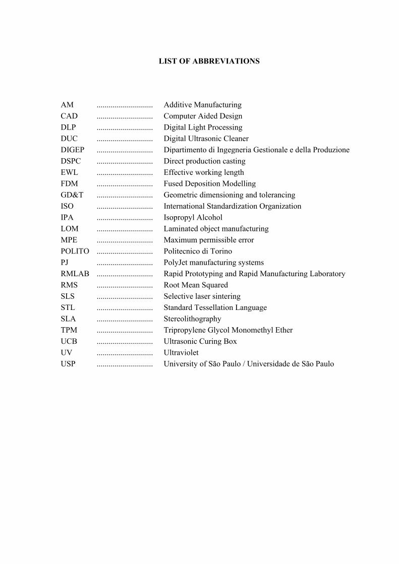
AM ............................ Additive Manufacturing CAD ............................ Computer Aided Design DLP ............................ Digital Light Processing DUC ............................ Digital Ultrasonic Cleaner DIGEP ............................ Dipartimento di Ingegneria Gestionale e della Produzione DSPC ............................ Direct production casting EWL ............................ Effective working length FDM ............................ Fused Deposition Modelling GD&T ............................ Geometric dimensioning and tolerancing ISO ............................ International Standardization Organization IPA ............................ Isopropyl Alcohol LOM ............................ Laminated object manufacturing MPE ............................ Maximum permissible error POLITO ............................ Politecnico di Torino PJ ............................ PolyJet manufacturing systems RMLAB ............................ Rapid Prototyping and Rapid Manufacturing Laboratory RMS ............................ Root Mean Squared SLS ............................ Selective laser sintering STL ............................ Standard Tessellation Language SLA ............................ Stereolithography TPM ............................ Tripropylene Glycol Monomethyl Ether UCB ............................ Ultrasonic Curing Box UV ............................ Ultraviolet USP ............................ University of São Paulo / Universidade de São Paulo

TABLE OF CONTENTS

1. INTRODUCTION 16

2. OBJECTIVE 19

3. ARTIFACT DEVELOPMENT 20

3.1 FORMERLY PROPOSED TEST ARTIFACTS 20

3.1.1 User Part Based Models 20

3.1.2 Moylan Based Models and Rules for Artifact Design 22

3.1.3 Other Test Artifacts 25

3.2 DESIGN POINTS OF INTEREST 26

3.2.1 Benchmarking Type Considerations 27

3.2.2 Stereolithography (SLA) machine used 27

3.2.3 Digital Light Processing (DLP) machine used 29

3.2.4 PolyJet technology machine used 30

3.2.5 Measurement equipment and design parameters 31

3.2.6 Geometries, features and part characteristics 35

3.2.6.1 Planes 36

3.2.6.2 Cylinders 37

3.2.6.3 Cones 38

3.2.6.4 Spheres 38

3.2.6.5 Prismatic Features 38

3.2.6.6 Derivative Characteristics 39

3.2.7 Error listing and analysis 39

3.3 THE PROPOSED PART 40

3.3.1 Dimensional Design 41

3.3.2 Selected Geometries 45

3.3.2.1 Concentric Cylinder Boss – Family A 45

3.3.2.2 Cylinder Boss – Family B 46

3.3.2.3 Pins – Family C 46

3.3.2.4 Hemisphere – Family D 47

3.3.2.5 Circular Holes – Family E 47

3.3.2.6 Square Boss – Family F 48

3.3.2.7 Horizontal Cylinders – Family G 48

3.3.2.8 Staircases – Family H 49

3.3.2.9 Inclines – Family I 50

3.3.2.10 Rectangular Boss – Family J 50

3.3.2.11 Cone – Family K 52

3.3.2.12 Outside Dimensions – Family L 52

3.3.2.13 Square Notches – Family M 53

3.3.3 Analyzed Derivative Characteristics 53

3.3.3.1 Concentricity and Vertical Cylinders – Family N and O 54

3.3.3.2 Horizontal Planar Surfaces of Interest – Family P 54

4. EXPERIMENTAL DEVELOPMENT 55

4.1 PREPARATION PROCEDURES 55

4.2 FABRICATION OF THE REPLICAS 57

4.2.1 Sharebot Rover and Antares – Fabrication description and detail 57

4.2.2 Stratasys Objet30 – Fabrication description and detail 59

4.2.3 Post-fabrication of the parts produced 61

4.2.4 Finished parts and expected results 63

4.3 MEASUREMENT PROCEDURE OF THE REPLICAS 65

4.3.1 Positioning and Fixation 66

4.3.2 Measurement strategy for standard geometries 66

4.3.3 CMM Calibration 71

5. ANALYSIS AND RESULTS 73

5.1 DIMENSIONAL ACCURACY IN IT GRADES 73

5.1.1 Stratasys Objet30 PolyJet – IT Grades for individual features 77

5.1.2 Sharebot Antares SLA – IT Grades for individual features 80

5.1.3 Sharebot Rover DLP– IT Grades for individual features 84

5.2 GEOMETRIC FEATURE ACCURACY ACCORDING TO GD&T STANDARDS 88

5.2.1 Form Specifications 88

5.2.2 Orientation and Location Specifications 92

5.2.3 Cones and spheres 96

5.3 ERROR ANALYSIS AND INSPECTION 98

5.3.1 Process Driven Issues 98

5.3.2 Inspection Driven Issues 103

6. CONCLUSION 104

REFERENCES 106

APPENDIX A – GEOMETRIC LABELING 112

APPENDIX B – SUMMARY OF RESINS 116

APPENDIX C – MANUFACTURING IMAGES 118

APPENDIX D – PHOTOS OF THE PRODUCED REFERENCE PARTS 126

16

1. INTRODUCTION

Throughout the years, society has repeatedly evolved in its ways of producing items

and goods. Recalling to Sir Isaac Newton’s much popularized metaphor: “If we’ve seen further,

it is by standing on the shoulders of giants [1]”. In its purest and earliest form, manufacturing,

or the production of objects for use or sale, saw commencement through artisanship, hand-

production methods, and a rural-based creation of items. By means of steadily improving

technology and a necessity of attending demands from flourishing populations, mechanization

and new manufacturing processes would emerge in Europe and the United States in the 18th

century with the Industrial Revolution [2]. Handwork and manual crafting would lose space

and product creation would transition into processes based in the usage of machinery and large

chemical operations. This can be categorized as the beginning of an “era of power”, where

human labor was incapable of being akin to the performance of steam or water powered

machinery. In the 19th century, with yet a second Industrial Revolution, work and energy

resources would once again migrate from its present state of affairs, into methods based in

combustible fuels and electricity. And finally, in the 20th century, robotics, automation and

electronics would make space for new, ground-breaking technologies [3].

Manufacturing methods would mature within this time, and eventually allow for

newly processed materials and the possibility of creating modernized products and goods. This

evolution can be comparatively observed through specific processes, such as injection molding,

for instance. The first machine of its type is a contemporary to the second Industrial Revolution:

an apparatus for pyroxiline manufacturing dating back to 1872 [4]. In contrast, by the second

half of the 20th century, plastic production had overtaken that of steel, and screw injection

machines would account for the vast majority of all injection molding machines – an unforeseen

technological scenario in earlier centuries. A synchronous, yet more accelerated comparison

can be made for another manufacturing method: in 1950, Raymond F. Jones conceptualized a

manufacturing procedure based on a “molecular spray” for a science fiction publisher [5]. Only

two decades later, the concept of polymerizing liquid monomers in a layer-by-layer fashion to

form solid objects was approached by David Jones, in a column from 1974 for a journal of

scientific content [6]. And this is the time frame and conjuncture in which additive

manufacturing processes would ultimately emerge.

Additive manufacturing is yet another technological advancement made possible

through society’s gathering of knowledge and expertise over time. It is a transformative method

in which computer-aided machines are capable of fabricating objects by means of material

17

deposition, usually in individual layers [7]. The first manifestations of additive manufacturing

emerged at around 1987, when the use of stereolithography (SLA) – a process of light-sensitive

liquid resin polymerization – became patented and commercially available. In the early ‘90s

alternative additive manufacturing processes would arise and also be commercialized, such as

laminated object manufacturing (LOM, 1991), fused deposition modelling (FDM, 1991),

selective laser sintering (SLS, 1992) and direct production casting (DSPC, 1993) [8]. Some of

these processes, such as SLA and SLS are still very prevalent in today’s market, and FDM itself

is responsible for the popularization of “3D printing” as a concept and as a readily available

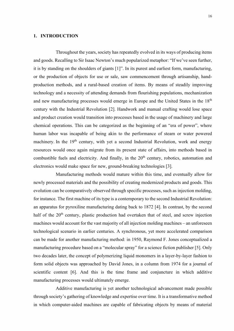
hobby-grade manufacturing process [9]. The ideation of new additive manufacturing processes

is constantly moving forward, and a timeline with the year in which these had emerged can be

seen in Figure 1 below.

Figure 1 – Timeline with a select amount of additive manufacturing processes, based on

patenting dates.

Source: [10]–[15]

Products made in 3D printing procedures such as FDM are known to be very

accessible, however, at the cost of some possibly problematic characteristics of the part, such

as mechanical resistance, material temperature traits or finishing quality. By opting to produce

a part through alternative additive manufacturing processes, it may be possible to achieve better

results within the selected attributes of the project. And that is where the field of fabrication

benchmarking becomes relevant. Ever so similar, each additive manufacturing procedure,

equipment or even configuration parameters will produce parts with individually distinctive

18

resulting characteristics. Therefore, it is important to carry out experimental observations of

objects fabricated and their attributes, in order to predict the results that can be obtained in a

specific manufacturing process.

In this dissertation, different machines and manufacturing processes available at

Politecnico di Torino (Turin, Italy) will be evaluated with regards to their capability of

producing parts with dimensional and geometric accuracy comparable to the CAD designs that

are presented for fabrication. Machines of three different manufacturing processes will be

evaluated within this study: stereolithography (SLA), digital light processing (DLP) and PolyJet

manufacturing processes. All of these processes are based on liquid resin photopolymers that

are cured in layers by the emission of ultraviolet light, in order to form a three-dimensional

object. A single test artifact model will be designed according to the boundary conditions of

the analysis, and manufactured in every machine. It is interesting to include in this test part a

range of different dimensions and basic geometric features.

According to Minetola et. al, when dealing with accuracy and tolerances, a

convenient method of analysis is that which is proposed by the standard International Tolerance

(IT) grades, proposed by the International Organization for Standardization (ISO) [16]. These

serve as a comparison reference for Geometric Dimensioning and Tolerancing (GD&T) of

different processes, and are capable of summarizing results of a benchmarking study for rapid

prototyping or additive manufacturing machines. After inspection of the replicas produced, it

will be possible to discriminate a measurable indicator for each machine, and therefore establish

which of the equipment at Politecnico di Torino is capable of producing a more accurately

correct three-dimensional object.

19

2. OBJECTIVE

The main objective of the dissertation at hand is to evaluate the dimensional and

geometric accuracy and manufacturing overall performance of three distinct additive

manufacturing machines available at Politecnico di Torino’s Rapid Prototyping and Rapid

Manufacturing Laboratory (RMLAB). The main constraint to the study is that each of the

manufacturing apparatuses analyzed must refer to a fabrication method based in the use of

photopolymers and resin-based curing of a 3D part. Within the direction of academic intent,

this thesis will commit to a detailed description of each manufacturing method approached by

the equipment available.

In order to create a GD&T benchmarking analysis of each machine, a reference

study of existing test artifacts must be conducted. This is done in order to ensure an efficient

part design that will allow for extraction of relevant fabrication parameters, and an overall

understanding of how engineering benchmarkings are structured for manufacturing processes.

As a concluding objective of the dissertation, the experimental data collected must be evaluated

with the intent of classifying each machine and process available at RMLAB with respect to

the relevant fabrication attributes selected.

20

3. ARTIFACT DEVELOPMENT

Accuracy performance of additive manufacturing and rapid prototyping machines

is evaluated through the dimensional and geometric accuracy of their manufactured parts.

Therefore, the process of selecting a part to be produced occupies an important role in

benchmarking studies of manufacturing equipment.

In this section, an in-depth analysis of existing reference parts and accuracy-related

topology will be conducted. Subsequently, the most feasible artifact solution is to be used in

the accuracy benchmarking study for the referred machines and processes.

3.1 Formerly proposed test artifacts

Various reference parts and artifact specimen have been proposed in previous

literature in an attempt to standardize and ensure completeness of benchmarking studies.

Throughout the years, researchers would add new geometric features and qualities to test parts

in order to compare the capabilities of various processes [17]. A group of diverse benchmarking

artifacts is analyzed below in order to determine which existing artifacts are interesting starting

points for working with SLA and other processes with photopolymers.

3.1.1 User Part Based Models

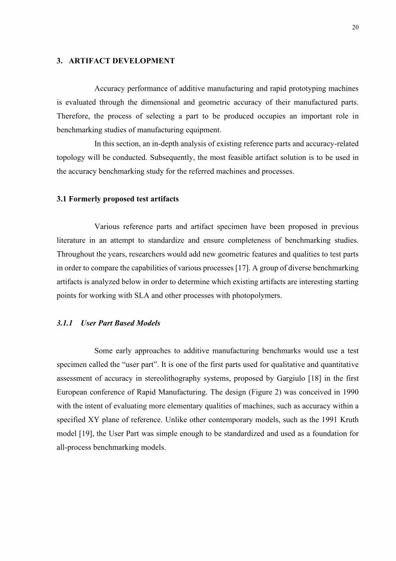
Some early approaches to additive manufacturing benchmarks would use a test

specimen called the “user part”. It is one of the first parts used for qualitative and quantitative

assessment of accuracy in stereolithography systems, proposed by Gargiulo [18] in the first

European conference of Rapid Manufacturing. The design (Figure 2) was conceived in 1990

with the intent of evaluating more elementary qualities of machines, such as accuracy within a

specified XY plane of reference. Unlike other contemporary models, such as the 1991 Kruth

model [19], the User Part was simple enough to be standardized and used as a foundation for

all-process benchmarking models.

21

Figure 2 – User part CAD model.

Source: [18]

This part has been used in benchmarks for stereolithography for as early as 1995

with Ippolito et. al [20], and the results of this analysis in the field have been used as a reference

for International Tolerance (IT) Grades for years.

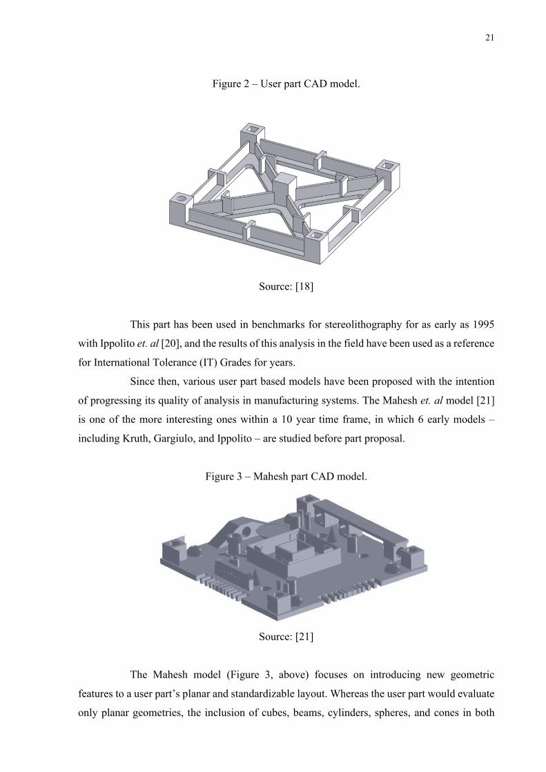
Since then, various user part based models have been proposed with the intention

of progressing its quality of analysis in manufacturing systems. The Mahesh et. al model [21]

is one of the more interesting ones within a 10 year time frame, in which 6 early models –

including Kruth, Gargiulo, and Ippolito – are studied before part proposal.

Figure 3 – Mahesh part CAD model.

Source: [21]

The Mahesh model (Figure 3, above) focuses on introducing new geometric

features to a user part’s planar and standardizable layout. Whereas the user part would evaluate

only planar geometries, the inclusion of cubes, beams, cylinders, spheres, and cones in both

22

solid and hollow configurations would corroborate completeness in geometric analysis. In order

to make the part standardizable, existing references of straightness (ISO 12780), roundness

(ISO 12181), flatness (ISO 12781), cylindricity (ISO 12180) and CMM standards were used in

the proposal.

The inclusion of multiple geometries became a tendency in artifact design, where

there was an approach of using standard 3D library features (such as spheres, cylinders, prisms,

cones, etc.). Part designers would be influenced by previous work and a common set of “rules”

seen in the field (see Section 3.1.2), and layouts would then preserve a rectangular or square

base with features that attempt to reproduce “real” geometries [17].

3.1.2 Moylan Based Models and Rules for Artifact Design

In 2012, Moylan et. al from the National Institute of Standards and Technology

(NIST - Gaithersburg, USA) reviewed existing test parts with the intention of proposing a new

artifact for standardization. The purpose of the study was to consolidate methodology that

would corroborate and facilitate the adoption of additive processes in functional and industrial

applications [17]. Therefore, working towards analyzing part accuracy, surface finish, process

speed and material proprieties can be kickstarted through standardizing a test part.

Throughout their work, Moylan et. al describe a set of “rules” for test artifact design.

Their analysis accounts for various considerations made in prior work, such as standards

proposed by Richter & Jacobs, Kruth and Byun. According to Moylan et. al, test artifact design

should [17]:

• Consider part sizing in order to test performance discrepancies near the edges

of the build platform as well as near its center;

• Have a substantial number of small, medium, and large features. If possible,

should attempt to determine a minimum feature size attainable;

• Not take too long to build;

• Not consume a large quantity of material;

• Be easy to measure;

• Emulate many features of a “real” part (e.g., thin walls, flat surfaces, holes, etc.);

• Include features along various different axes;

• Have simple geometrical shapes, allowing perfect definition and easy control of

the geometry;

23

• Require minimal post-treatment or manual intervention if possible (i.e.: no

support structures);

• Allow repeatability measurements;

These “rules” consist of recommendations and good practices in order to allow for

analysis completeness. In some cases, however, it is optimal to observe different scenarios to

which a part is subjected, allowing for design flexibility in this subject.

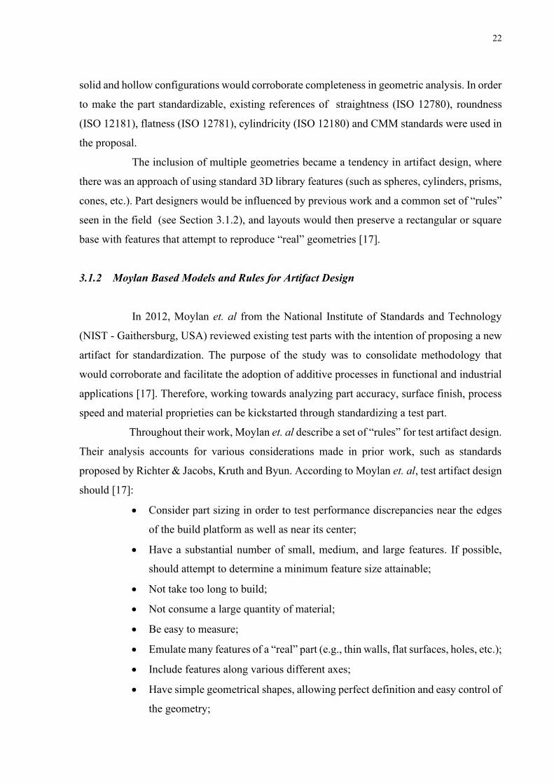
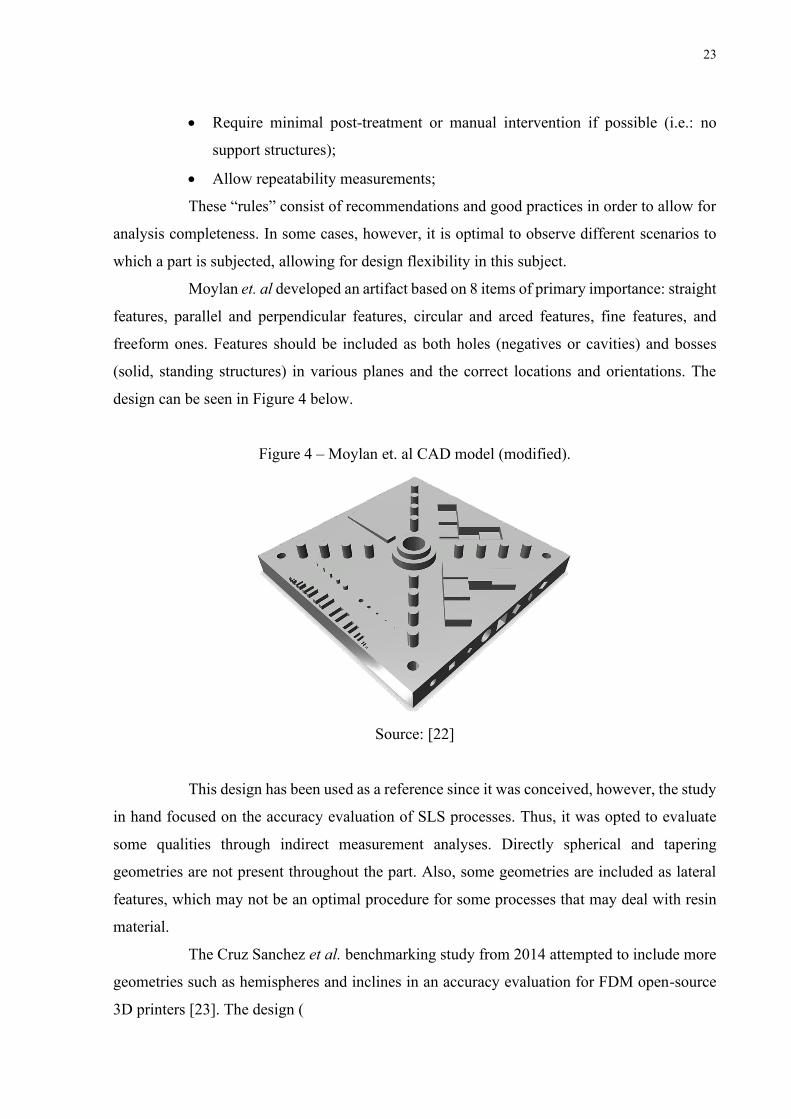
Moylan et. al developed an artifact based on 8 items of primary importance: straight

features, parallel and perpendicular features, circular and arced features, fine features, and

freeform ones. Features should be included as both holes (negatives or cavities) and bosses

(solid, standing structures) in various planes and the correct locations and orientations. The

design can be seen in Figure 4 below.

Figure 4 – Moylan et. al CAD model (modified).

Source: [22]

This design has been used as a reference since it was conceived, however, the study

in hand focused on the accuracy evaluation of SLS processes. Thus, it was opted to evaluate

some qualities through indirect measurement analyses. Directly spherical and tapering

geometries are not present throughout the part. Also, some geometries are included as lateral

features, which may not be an optimal procedure for some processes that may deal with resin

material.

The Cruz Sanchez et al. benchmarking study from 2014 attempted to include more

geometries such as hemispheres and inclines in an accuracy evaluation for FDM open-source

3D printers [23]. The design (

24

Figure 5) is a modified version of the Moylan et al. 2012 standardized part, that includes 15

different family groups labeled through a lettering system (A-O) and a number for each

individual geometry.

Figure 5 – Cruz Sanchez et al. CAD Model with identification ID’s.

Source: [23]

Within a different configuration setup, Minetola’s benchmarking study for additive

manufacturing systems uses a similar concept to that of Cruz Sanchez and Moylan. A planar

base is used in a square or rectangular setup with the inclusion of various geometries (Figure

6). It is very interesting to observe how efficiently Minetola et al. places each elements within

the available space. Cruz Sanchez and Minetola attempt to create a special configuration that

would satisfy the good practices of minimizing material waste – through an efficient

geometries-over-area ratio – while still contemplating CMM limitations [16].

Minetola’s approach to improving geometry allocation also uses a concept of

element division into a negative (hollow half), and positive half (bosses). This is noticeable in

geometries such as hemispheres (SPi) and horizontal cylinders (CLi), where the same space that

would be occupied by a full feature is optimized into containing two versions of a measurable

element. This is a functioning method due to the fact that CMM measurements are results of

interpolated measurement data, and therefore a full feature is not indispensable – only enough

points of interpolation are mandatory [24]. It is also interesting to notice how tilted planes can

be found in almost every derivative feature of the part (TPi).

25

Figure 6 – Minetola et al. CAD Model with identifications.

Source: [16]

3.1.3 Other Test Artifacts

A contemporary analysis to that of Moylan et al. is the Fahad & Hopkinson study

also performed in 2012 [25]. In this research, various existing parts are analyzed and compared

in terms of their principal functionalities and benchmarking results. Among others, the

mentioned models of Kruth, Mahesh and Ippolito are observed as adequate, however each with

correlated limitations. An interesting analyzed model is that of Juster & Childs [26], where the

concept of free-form geometries is included, as seen in Figure 7. However, due to difficult

standardization, symmetry and repeatability, this concept can be seen as a limitation to model

designs.

Figure 7 – Juster & Childs CAD Model.

Source: [25]

26

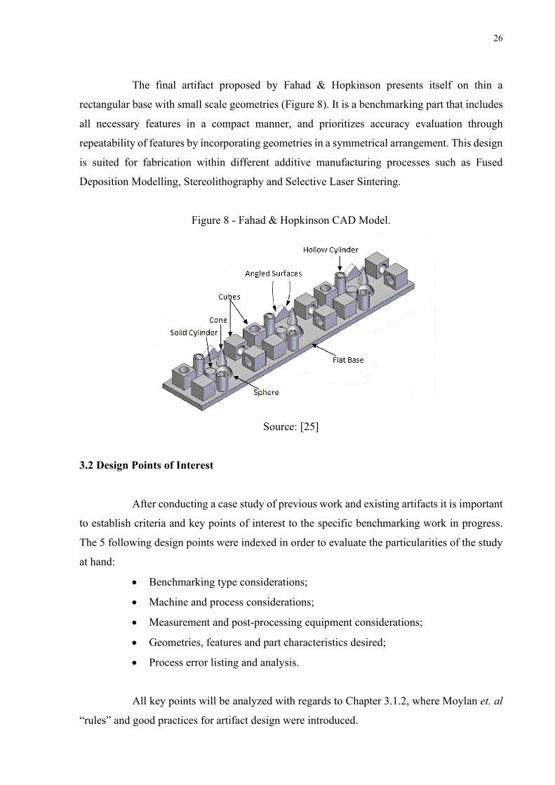
The final artifact proposed by Fahad & Hopkinson presents itself on thin a

rectangular base with small scale geometries (Figure 8). It is a benchmarking part that includes

all necessary features in a compact manner, and prioritizes accuracy evaluation through

repeatability of features by incorporating geometries in a symmetrical arrangement. This design

is suited for fabrication within different additive manufacturing processes such as Fused

Deposition Modelling, Stereolithography and Selective Laser Sintering.

Figure 8 - Fahad & Hopkinson CAD Model.

Source: [25]

3.2 Design Points of Interest

After conducting a case study of previous work and existing artifacts it is important

to establish criteria and key points of interest to the specific benchmarking work in progress.

The 5 following design points were indexed in order to evaluate the particularities of the study

at hand:

• Benchmarking type considerations;

• Machine and process considerations;

• Measurement and post-processing equipment considerations;

• Geometries, features and part characteristics desired;

• Process error listing and analysis.

All key points will be analyzed with regards to Chapter 3.1.2, where Moylan et. al

“rules” and good practices for artifact design were introduced.

27

3.2.1 Benchmarking Type Considerations

A benchmark is a comparison of performance in similar yet different organized

structures (such as companies machines, equipment, processes etc.). Such comparison requires

a reference standard with regards to which structural aspects are being observed. In mechanical

engineering, benchmarkings can be used to contrast material proprieties, manufacturing

accuracy, finishing, repeatability, geometrical resolution and even design or working conditions

of parts [25]. According to Mahesh et al., benchmarkings in additive manufacturing can be

classified within three categories:

• Process Benchmark: used to establish process related parameters (part

orientation, support structures, layer thickness, speed, etc.).

• Mechanical Benchmark: used to analyze the mechanical properties (tensile

strength, compressive strength, creep, etc.);

• Geometric Benchmark: used to measure the geometric features of a part (i.e.

tolerances, accuracy, repeatability and surface finish);

Within this dissertation, a geometric benchmarking will be realized in order to

evaluate the accuracy and tolerances of parts produced by additive manufacturing processes

and machines in stereolithography (SLA), digital light processing (DLP) and PolyJet

equipment. Therefore, the test part’s design should focus on optimizing observability of

characteristics such as finishing, tolerances and geometric accuracy.

3.2.2 Stereolithography (SLA) machine used

The first machine benchmarked in this study will be the Sharebot Antares. Sharebot

is an Italian based company that offers AM technology services in FDM, resin-based

manufacturing and powder sintering. The Antares is one of their older product models in

photosensitive resin-based manufacturing. The printer is categorized as a high-precision

professional SLA working tool for large model fabrication. Further details about the machine

can be found in Table 1 below.

28

Table 1 – Sharebot Antares printer specifications.

ANTARES TECHNICAL DETAILS Materials PR-S, PR-T Printing Volume 250 x 250 x 250 mm XY resolution Layer ±0.1 mm (100 micron) Layer thickness > 0,05 mm Laser Power 150 mW Wavelength 405 nm Dimensions 500 x 500 x 1.400 mm Weight 120 kg Slicing software Included

Source: [27]

At first, it is important to be aware of the machine’s size. Since the print volume is

of 250 𝑥 250 𝑥 250 𝑚𝑚 and the Sharebot Antares is a fairly large machine (Figure 9),

dimensional limitations are not very concerning in terms of artifact design. As observed by

Moylan et al. existing test artifacts have considerable size variations, however the largest

observed part was of 240 𝑥 240 𝑚𝑚 in a square-based XY area [17].

Figure 9 - Sharebot Antares SLA printer.

Source: [28]

29

3.2.3 Digital Light Processing (DLP) machine used

For this study, the equipment observed will be the Sharebot Rover DLP Printer

(Figure 10). The Sharebot Rover is a machine that proposes compact desktop manufacturing.

Therefore, this machine contains a small scale printing plate of only 62 𝑥 115 𝑥 100 𝑚𝑚 [29],

which is a relevant parameter in order to define the maximum admissible build volume for a

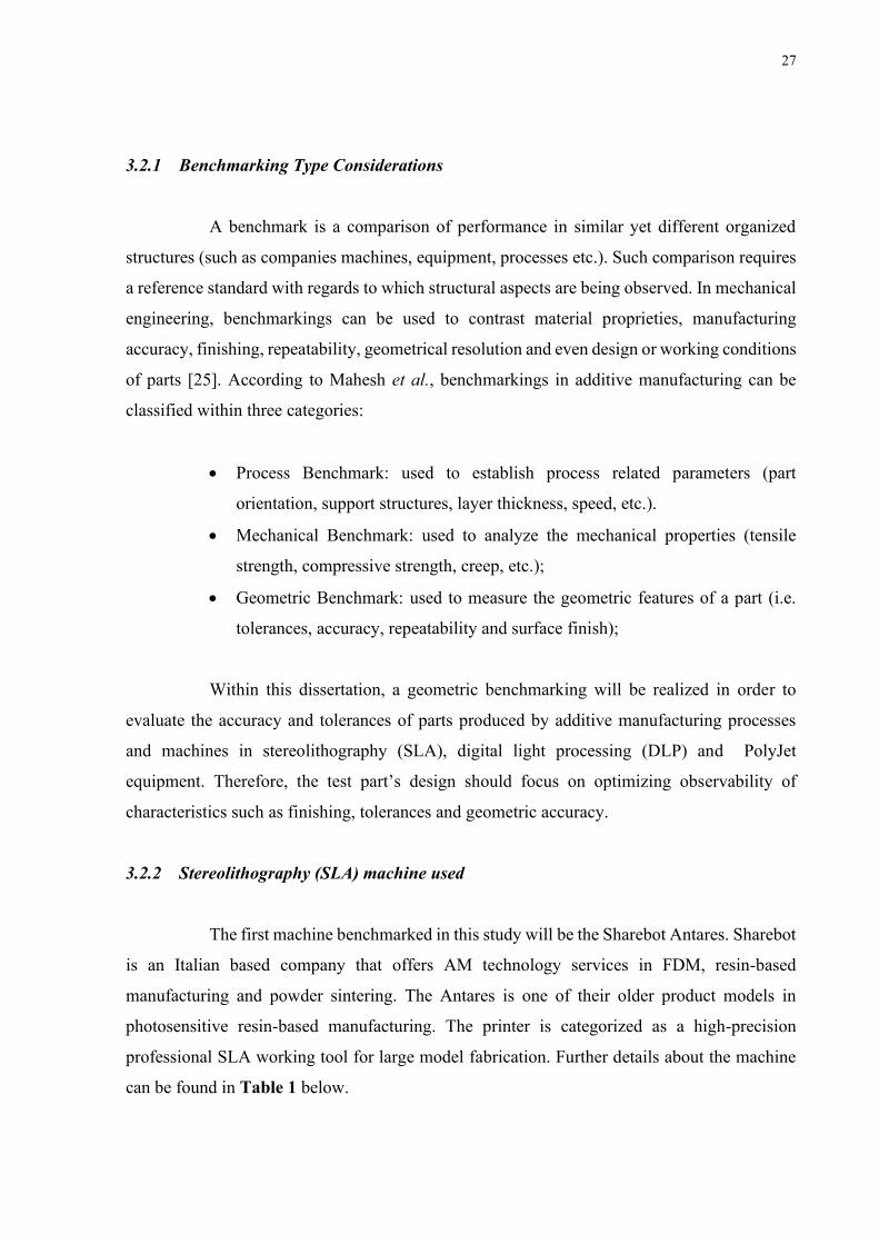
test artifact. Further details about the Sharebot Rover can be found in Table 2 below.

Table 2 – Sharebot Rover printer specifications.

ROVER TECHNICAL DETAILS Materials ASTM, S-Series Printing area XY 62 x 115 x 100 mm XY resolution Layer 47 micron Layer thickness 20 - 100 micron Matrix 2K 1440 x 2560 pixels Wavelength 405 nm Dimensions 460x353x200 mm Weight 15 kg Slicing software Included

Source: [29]

Figure 10 – Sharebot Rover DLP printer.

Source: [29]

30

3.2.4 PolyJet technology machine used

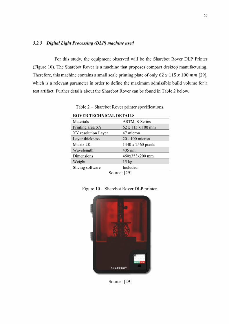
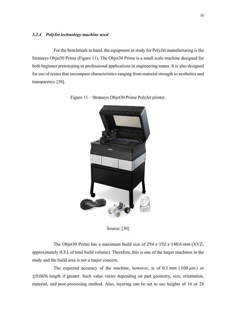
For the benchmark in hand, the equipment in study for PolyJet manufacturing is the

Stratasys Objet30 Prime (Figure 11). The Objet30 Prime is a small scale machine designed for

both beginner prototyping or professional applications in engineering teams. It is also designed

for use of resins that encompass characteristics ranging from material strength to aesthetics and

transparency [30].

Figure 11 – Stratasys Objet30 Prime PolyJet printer.

Source: [30]

The Objet30 Prime has a maximum build size of 294 𝑥 192 𝑥 148.6 𝑚𝑚 (XYZ;

approximately 8.3 𝐿 of total build volume). Therefore, this is one of the larger machines in the

study and the build area is not a major concern.

The expected accuracy of the machine, however, is of 0.1 𝑚𝑚 ( 100 𝜇𝑚 ) or

±0.06% length if greater. Such value varies depending on part geometry, size, orientation,

material, and post-processing method. Also, layering can be set to use heights of 16 or 28

31

microns, which will also influence the final part precision [31]. Further information about the

printer is summarized in Table 3 below.

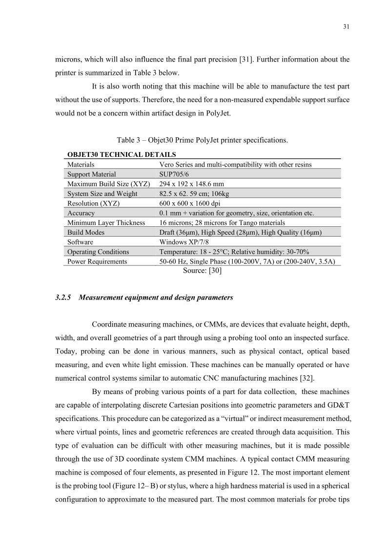
It is also worth noting that this machine will be able to manufacture the test part

without the use of supports. Therefore, the need for a non-measured expendable support surface

would not be a concern within artifact design in PolyJet.

Table 3 – Objet30 Prime PolyJet printer specifications.

OBJET30 TECHNICAL DETAILS Materials Vero Series and multi-compatibility with other resins Support Material SUP705/6 Maximum Build Size (XYZ) 294 x 192 x 148.6 mm System Size and Weight 82.5 x 62. 59 cm; 106kg Resolution (XYZ) 600 x 600 x 1600 dpi Accuracy 0.1 mm + variation for geometry, size, orientation etc. Minimum Layer Thickness 16 microns; 28 microns for Tango materials Build Modes Draft (36μm), High Speed (28μm), High Quality (16μm) Software Windows XP/7/8 Operating Conditions Temperature: 18 - 25°C; Relative humidity: 30-70% Power Requirements 50-60 Hz, Single Phase (100-200V, 7A) or (200-240V, 3.5A)

Source: [30]

3.2.5 Measurement equipment and design parameters

Coordinate measuring machines, or CMMs, are devices that evaluate height, depth,

width, and overall geometries of a part through using a probing tool onto an inspected surface.

Today, probing can be done in various manners, such as physical contact, optical based

measuring, and even white light emission. These machines can be manually operated or have

numerical control systems similar to automatic CNC manufacturing machines [32].

By means of probing various points of a part for data collection, these machines

are capable of interpolating discrete Cartesian positions into geometric parameters and GD&T

specifications. This procedure can be categorized as a “virtual” or indirect measurement method,

where virtual points, lines and geometric references are created through data acquisition. This

type of evaluation can be difficult with other measuring machines, but it is made possible

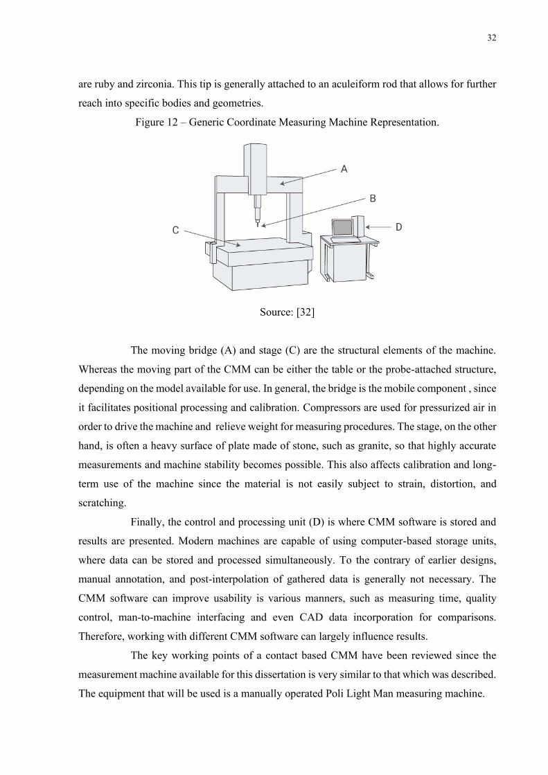
through the use of 3D coordinate system CMM machines. A typical contact CMM measuring

machine is composed of four elements, as presented in Figure 12. The most important element

is the probing tool (Figure 12– B) or stylus, where a high hardness material is used in a spherical

configuration to approximate to the measured part. The most common materials for probe tips

32

are ruby and zirconia. This tip is generally attached to an aculeiform rod that allows for further

reach into specific bodies and geometries.

Figure 12 – Generic Coordinate Measuring Machine Representation.

Source: [32]

The moving bridge (A) and stage (C) are the structural elements of the machine.

Whereas the moving part of the CMM can be either the table or the probe-attached structure,

depending on the model available for use. In general, the bridge is the mobile component , since

it facilitates positional processing and calibration. Compressors are used for pressurized air in

order to drive the machine and relieve weight for measuring procedures. The stage, on the other

hand, is often a heavy surface of plate made of stone, such as granite, so that highly accurate

measurements and machine stability becomes possible. This also affects calibration and long-

term use of the machine since the material is not easily subject to strain, distortion, and

scratching.

Finally, the control and processing unit (D) is where CMM software is stored and

results are presented. Modern machines are capable of using computer-based storage units,

where data can be stored and processed simultaneously. To the contrary of earlier designs,

manual annotation, and post-interpolation of gathered data is generally not necessary. The

CMM software can improve usability is various manners, such as measuring time, quality

control, man-to-machine interfacing and even CAD data incorporation for comparisons.

Therefore, working with different CMM software can largely influence results.

The key working points of a contact based CMM have been reviewed since the

measurement machine available for this dissertation is very similar to that which was described.

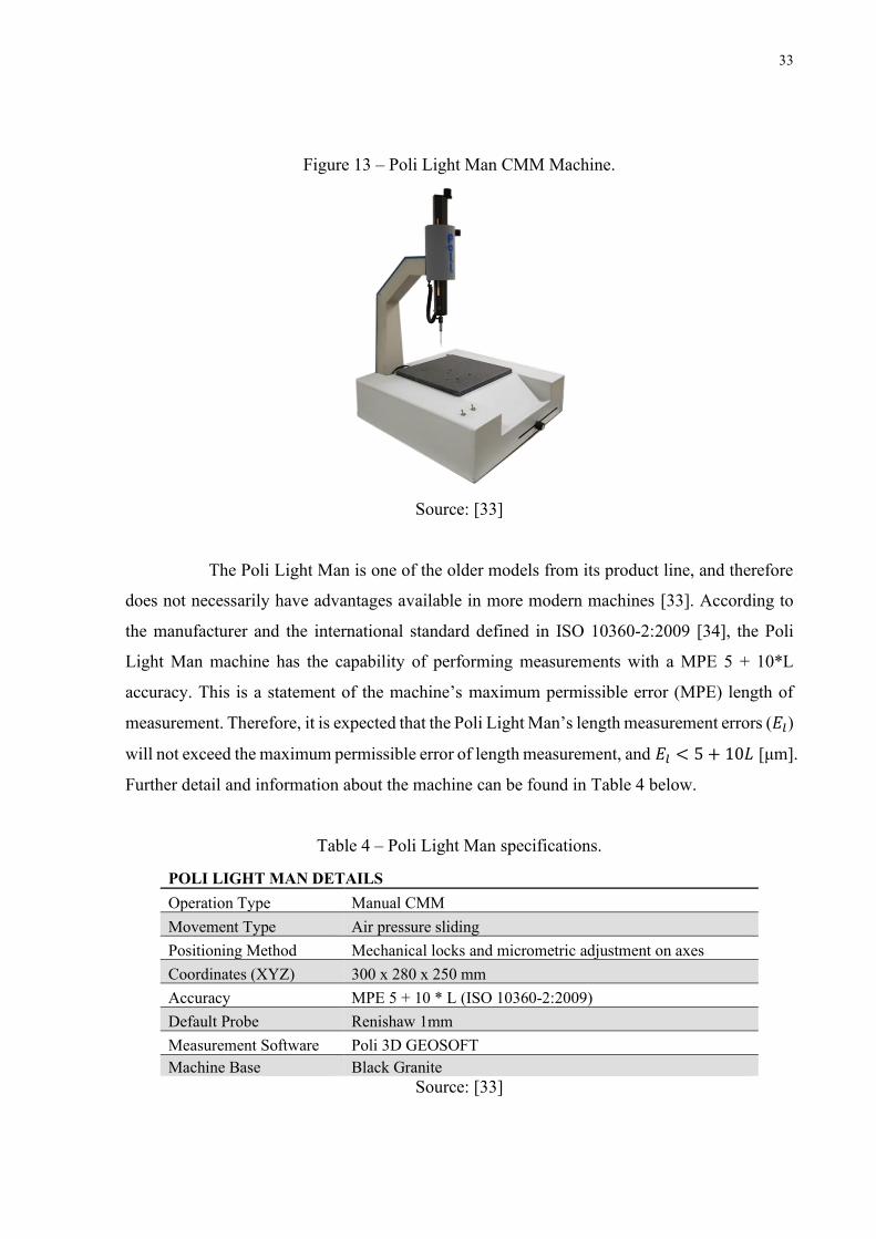
The equipment that will be used is a manually operated Poli Light Man measuring machine.

33

Figure 13 – Poli Light Man CMM Machine.

Source: [33]

The Poli Light Man is one of the older models from its product line, and therefore

does not necessarily have advantages available in more modern machines [33]. According to

the manufacturer and the international standard defined in ISO 10360-2:2009 [34], the Poli

Light Man machine has the capability of performing measurements with a MPE 5 + 10*L

accuracy. This is a statement of the machine’s maximum permissible error (MPE) length of

measurement. Therefore, it is expected that the Poli Light Man’s length measurement errors (𝐸𝑙)

will not exceed the maximum permissible error of length measurement, and 𝐸𝑙 < 5 + 10𝐿 [μm].

Further detail and information about the machine can be found in Table 4 below.

Table 4 – Poli Light Man specifications.

POLI LIGHT MAN DETAILS Operation Type Manual CMM Movement Type Air pressure sliding Positioning Method Mechanical locks and micrometric adjustment on axes Coordinates (XYZ) 300 x 280 x 250 mm Accuracy MPE 5 + 10 * L (ISO 10360-2:2009) Default Probe Renishaw 1mm Measurement Software Poli 3D GEOSOFT Machine Base Black Granite

Source: [33]

34

Another measurement parameter of the CMM that is relevant for part design is that

of the stylus to be used. Styli are the tips of probing tools in contact coordinate measuring

machines, where a measuring rod with a spherical head attached to its extremity makes physical

contact to the component under measurement [35].

Choosing a stylus is of paramount importance for artifact design in terms of

geometric and dimensional decision making. General stylus selection practices recommend

short non-jointed styli with spherical sizing specific to the type of analysis in hand. The length

of a stylus influences in errors due to material deflection. A longer stylus is prone to deflection

or bending, inducing errors that can be minimized through the usage of a shorter stylus overall

length. The same principle can be applied to jointed styli, where builds that contain joints or

extensions can induce deflection points and localized movement error. Finally, the diameter of

the probing sphere influences how contact affects readings. Larger spheres maximize clearance

from the part, reducing false triggering, while a smaller probe will maximize the impact of

surface finishing and imprecision. A general overview of relevant stylus parameters can be seen

in Figure 14 below, such as its threading (A), effective working length (B), overall length (L)

and diameter (D).

Figure 14 – Stylus dimensions for terminology.

Source: [35]

For a benchmarking study that assesses dimensional precision and geometric

accuracy, and especially one within additive manufacturing, it is important to use a small

enough spherical probing tip. This will allow for examination of the parts inaccuracies due to

surface roughness, building precision, layering, among other factors. Therefore, the preeminent

parameters of the stylus to be evaluated are its diameter and effective working length.

Each stylus has an Effective Working Length (EWL, represented as “B” in Figure

14), which is expected the working length of the stylus, regarding its possible penetration into

part geometries [24]. This length is measured as that to which the tip can achieve before the

35

stylus shaft can contact the component, as seen in Figure 15. However, this dimension includes

the tapered cone frustrum used in the shaft, and for very small parts, it may be more relevant to

consider only the stylus’ rod length.

Figure 15 – Effective working length of a measuring probe.

Source: [24]

The stylus available at Politecnico di Torino for this study is a ruby-point 1mm

Renishaw spherical probe, as referenced earlier in Table 4. It has an EWL of 12 𝑚𝑚, composed

by a 7 𝑚𝑚 rod and tapered cone. Therefore, artifact design should consider a maximum depth

of the rod length for geometries in the vertical Z axis.

Figure 16 – Renishaw 1mm probing tool at Politecnico di Torino.

3.2.6 Geometries, features and part characteristics

As seen in the references study, a manufacturing benchmark will use a reference

part with specific geometries that evaluate different types of machine characteristics.

Geometries will vary from simple, linear shapes, to those that are composed of tapered or free-

form elements. In this chapter, the geometries seen in past work will be analyzed as to their

36

purposes, limitations and what are the expected analytical results that each element will offer

to an additive manufacturing benchmark.

It is also important to note that some benchmarking attributes are not necessarily

geometries, but a derivative of the interaction between equal geometries or diverging ones. A

clear example can be that of parallelism. This is a part characteristic that is evaluated through a

specific hypothetically perfect reference. Concentricity is another characteristic that also

demands a referencing circumference, and is associated to geometrical elements such as circular

holes and embossed cylinders. This type of part characteristic is useful for manufacturing

benchmarking, however, is not generally be considered as a geometric element, but a featured

by-product.

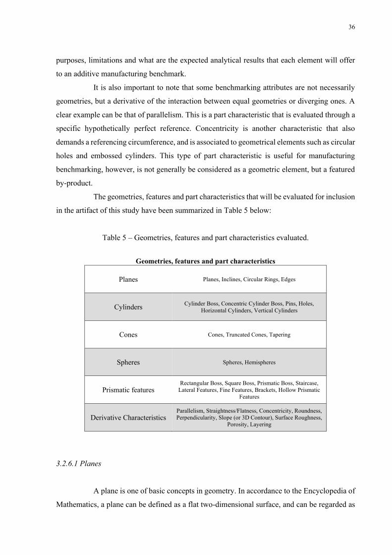
The geometries, features and part characteristics that will be evaluated for inclusion

in the artifact of this study have been summarized in Table 5 below:

Table 5 – Geometries, features and part characteristics evaluated.

Geometries, features and part characteristics

Planes Planes, Inclines, Circular Rings, Edges

Cylinders Cylinder Boss, Concentric Cylinder Boss, Pins, Holes, Horizontal Cylinders, Vertical Cylinders

Cones Cones, Truncated Cones, Tapering

Spheres Spheres, Hemispheres

Prismatic features Rectangular Boss, Square Boss, Prismatic Boss, Staircase,

Lateral Features, Fine Features, Brackets, Hollow Prismatic Features

Derivative Characteristics Parallelism, Straightness/Flatness, Concentricity, Roundness, Perpendicularity, Slope (or 3D Contour), Surface Roughness,

Porosity, Layering

3.2.6.1 Planes

A plane is one of basic concepts in geometry. In accordance to the Encyclopedia of

Mathematics, a plane can be defined as a flat two-dimensional surface, and can be regarded as

37

a set of points, a set of straight lines, a combination of a point to an axis, among other

mathematical axioms and definitions. In practice, however, a plane will be defined as a finite

surface that will likely contain imperfections and inaccuracies, such as a natural roughness and

meager curvature.

As seen in formerly examined bibliography, in terms of manufacturing benchmarks,

planes are an important feature that will be present in most formerly proposed artifact elements,

and naturally derive off of other geometries as well. Therefore, a plane will be seen as a

geometric configuration that is capable of evaluating secondary derivative attributes such as

flatness, parallelism, perpendicularity, sloping, and general features involving angularity. As

will be further detailed in Chapter 4, planar features are also an important element for CMM

calibration.

In artifact design, planes may be presented in various configurations, such as the

contrast between a standard vertically oriented feature to a horizontal one. In terms of form,

planes may be present in different geometries, due to the nature of prismatic elements, which

will be listed in the upcoming chapters. A plane will naturally derive off of geometric extrusions,

being available for evaluation atop of embossed features, walls, hollow features, and holes.

3.2.6.2 Cylinders

Cylindricity is an important feature to be evaluated in manufacturing

benchmarkings. Physicist Eric Weisstein defines the term “cylinder” as effective for either a

mathematical surface that is bound within two planes, and a solid that would be enclosed by

this very generalized cylinder [36]. This last definition can also be categorized as a prism in

itself. However, in practice, cylinders can be presented in various forms: different orientations,

embossed, hollow, holes, among, quarter cylinders, etc. As presented Table 5, there are many

possible configurations to a cylindric geometry, and for practical reason, a cylinder will be

categorized as a general geometry formed by means of a hypothetical integral displacement of

a circumference, filled or in contours.

The objective of a cylindric feature in a manufacturing benchmark is that of

evaluating the machines capability of producing cylinders and circular features. A feature’s

cylindricity (“circular straightness”) can be used to evaluate error and alignment within the

machines axes. Other factors such as roundness, axial positioning, capability of producing radii,

coaxiality and repeatability can all be evaluated through the use of cylinders and combined

circular features.

38

3.2.6.3 Cones

According to ISO 3040:2016 cones are a product of a right-angle rotated triangle,

where any intersection by a plane perpendicular to the axis of the nominal cone is a circle [37].

The truncated cone that is represented by the standard is characterized by a finite length that

connects a point (or cone tip) to its base circumference, with the largest possible radius in the

feature.

Cones are an interesting feature to be analyzed since they are largely subject to

different types of errors that may occur in additive manufacturing, such as the “staircase effect”

and “missing features” effect (further detail in Chapter 5.3.1). This feature, however, is not

largely evaluated in prior bibliography in terms of its performance in IT Grades.

3.2.6.4 Spheres

Some industries are interested in fabricating spherical parts or components with

spherical features in additive manufacturing, such as businesses related to roller bearings that

may be concerned about weight, tolerances, or material performance [38]. Spheres can be

defined as “a solid figure that is completely round, with every point on its surface at an equal

distance from the center”, according to the Oxford dictionary [39].

For the purpose of a benchmarking, there is little research on the evaluation of

accuracy for spherical features in additive manufacturing. This feature can be used for the

definition of precision in circular dimensions for IT Grades, and can evaluate how likely the

machine or process is to produce a three-dimensional spherical object. This geometry can be

included in artifact design as a probe-like supported sphere or truncated sphere, and in the latter

case the approach used by Minetola et. al of including hemispheres or quarter-spheres is

recommended for conciseness and optimization of base area.

3.2.6.5 Prismatic Features

Prismatic features can be understood as “a solid figure with ends that are parallel

and of the same size and shape, and with sides whose opposite edges are equal and parallel”.

Therefore, this feature encompasses extrusions such as: rectangular bosses, square bosses,

39

triangular bosses, solid cylinders (circular boss), and other features that would only require the

protrusion of a basic shape.

These features can be utilized in order to evaluate flatness, circularity, parallelism,

the capability of producing parts with correct heights, and the capacity of creating small or fine

features. Thus, this is an interesting feature to be included in artifact design, since various data

points can be extracted from a single feature in measurement and analysis.

3.2.6.6 Derivative Characteristics

As mentioned in Chapter 3.2.1 manufacturing benchmarkings can evaluate various

capabilities of a machine or process. Characteristics such as part strength, repeatability, time

until fabrication, etc. are evaluated in this type of study, and in a geometric benchmarking the

inclusion of specific geometries and features enables the inspection of derivative characteristics

that depend on one or more features.

Parallelism can be evaluated between opposing planes and can indicate how

consistent the process is in terms of fabricating a part with correctly oriented geometries.

Similarly, flatness and straightness can be evaluated in terms of how accurate the production of

planes and lines are, respectively. And in identical fashion, quality of layering and the surface

roughness obtained are important parameters for manufacturers. In terms of circular features,

concentricity and roundness can be evaluated in features that have radii as their primary

dimensional parameter. Finally, sloping and angularity are characteristics that are interestingly

observed in benchmarkings, due to recurrent errors in additive manufacturing such as the

“staircase effect”.

3.2.7 Error listing and analysis

In rapid prototyping there are various characteristics of fabrication that may affect

part accuracy. According to a classification by W. Cheng et al. there are six sources of errors

during the building of a part: Tessellation; Missing feature errors; Overcure; Distortion and

shrinkage; The “container effect”; and the “staircase effect” [40].

Tessellation – the initial source of errors listed – is an effect caused by the

conversion of a computerized model into a fabricated part. Most CAD packages generally

construct parts using mathematical representation, which allows for continuity, but slicing

software creates layers based on an approximated triangulation of mesh data in STL files. This

40

problem can be alleviated by using other file formats. “Missing feature” is an effect related to

constant slicing thickness and fabrication over a singular layer height. Since elements may not

be multiples of layer thickness, this effect amounts to potential negligence of geometrical

features of the part, and hence results in a loss of control over the accuracy of the manufactured

part [41]. Overcure, also known as cure-through or the “back-side effect”, refers to errors

caused by unaccounted-for light propagation, that may cause undesired curing in incorrect

zones [42]. Distortion and shrinkage are related to material proprieties, topology of the

fabricated part and the usage of support structures. The “container effect” is related to surface

tension generated around an enclosed region, which would not allow for draining of retained

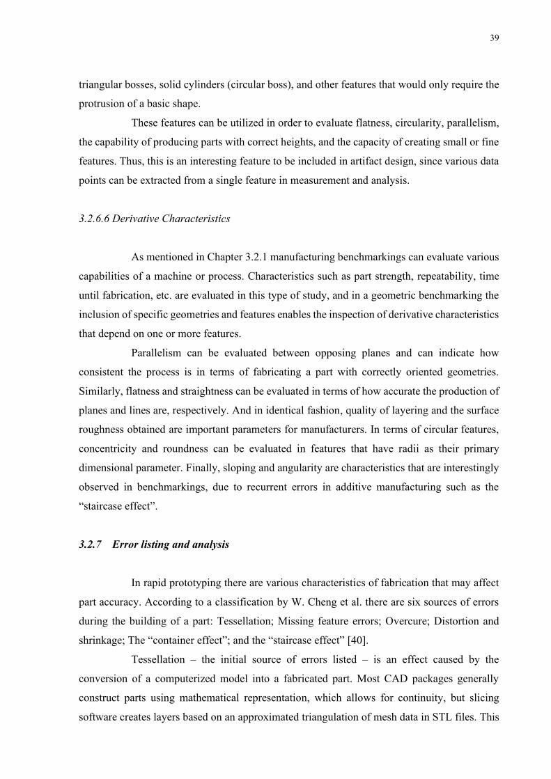
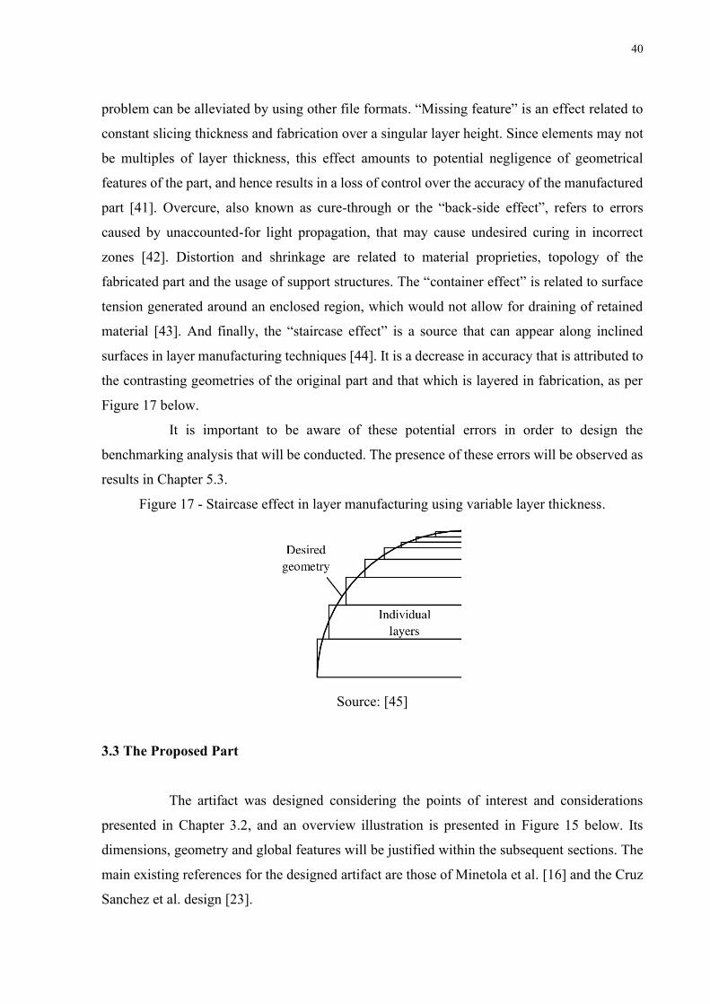
material [43]. And finally, the “staircase effect” is a source that can appear along inclined

surfaces in layer manufacturing techniques [44]. It is a decrease in accuracy that is attributed to

the contrasting geometries of the original part and that which is layered in fabrication, as per

Figure 17 below.

It is important to be aware of these potential errors in order to design the

benchmarking analysis that will be conducted. The presence of these errors will be observed as

results in Chapter 5.3.

Figure 17 - Staircase effect in layer manufacturing using variable layer thickness.

Source: [45]

3.3 The Proposed Part

The artifact was designed considering the points of interest and considerations

presented in Chapter 3.2, and an overview illustration is presented in Figure 15 below. Its

dimensions, geometry and global features will be justified within the subsequent sections. The

main existing references for the designed artifact are those of Minetola et al. [16] and the Cruz

Sanchez et al. design [23].

41

Figure 18 – Proposed artifact part.

3.3.1 Dimensional Design

As seen in sections Benchmarking Type Considerations, Stereolithography (SLA)

machine used and Digital Light Processing (DLP) machine used, each machine has dimensional

limitations that must be considered within the artifact design. A first approach to the conception

of a test part must be done regarding its principal outer dimensions. As seen in Chapter 3.2.3,

the Digital Light Processing machine (Sharebot Rover) has a printing area of 62 x 115 x 100

mm. Therefore, the Rover is composed by the smallest available build platform, and this will

be the main dimensional restriction of the test piece.

Since additive manufacturing processes are based in a successive deposition of

material layers, most times there is a necessity for the use of supporting structures, which can

be considered in artifact design. A model may contain bridges – structures that are not supported

and connect two sides of the same part – or overhangs – non-supported, drawn-out extremities

(Figure 19). However, it is a general rule of thumb that not all overhangs and bridges require

supports. Considering that there is an imperceptible offset in the stacking of consecutive layers,

it is possible to produce overhangs that are not overly tilted with respect to the vertical axis.

Any geometry that has an angle below 45 degrees to the Z axis can be supported by previously

produced layers [46]. Therefore, it is important to consider a potentially tilted artifact when

establishing artifact dimensions.

42

Figure 19 – Comparison between 45° and 90° overhangs and supporting necessities.

Source: [46]

Additionally, an angled artifact and even the prioritization of using support

structures may be an interesting consideration in some resin-based additive manufacturing

processes.

Having stated these boundary conditions for the sizing problem of the artifact, it is

finally possible to consider its outer dimensions and design. A rectangular shaped base was

arbitrarily selected for simplicity and clarity of dimensional calculation.

Figure 20 illustrates the dimensional analysis for the artifact part being positioned in a generic

arrangement, and (1) states the length 𝐿𝑖 = 𝐿(𝑖) as a function of a possible axis 𝑖 = {𝑥, 𝑦, 𝑧},

where it is assumed 𝑥 ≥ 𝑦 ≫ 𝑧:

𝐿𝑖 = 𝑖 ∗ 𝑐𝑜𝑠(𝜃) + 𝑧 ∗ 𝑐𝑜𝑠(𝜃 −

𝜋

2) (1)

Figure 20 – Generic arrangement of the part with regards to the build tray.

43

𝐿𝑥 = 𝑥 ∗ 𝑐𝑜𝑠(𝜃) + 𝑧 ∗ 𝑐𝑜𝑠 (𝜃 −

𝜋

2) < 115 𝑚𝑚 (2)

𝐿𝑦 = 𝑦 ∗ 𝑐𝑜𝑠(𝜃) + 𝑧 ∗ 𝑐𝑜𝑠 (𝜃 −

𝜋

2) < 62 𝑚𝑚 (3)

𝐿𝑧 = 𝑥 ∗ 𝑠𝑖𝑛(𝜃) + 𝑧 ∗ 𝑠𝑖𝑛 (𝜃 −

𝜋

2) < 100 𝑚𝑚 (4)

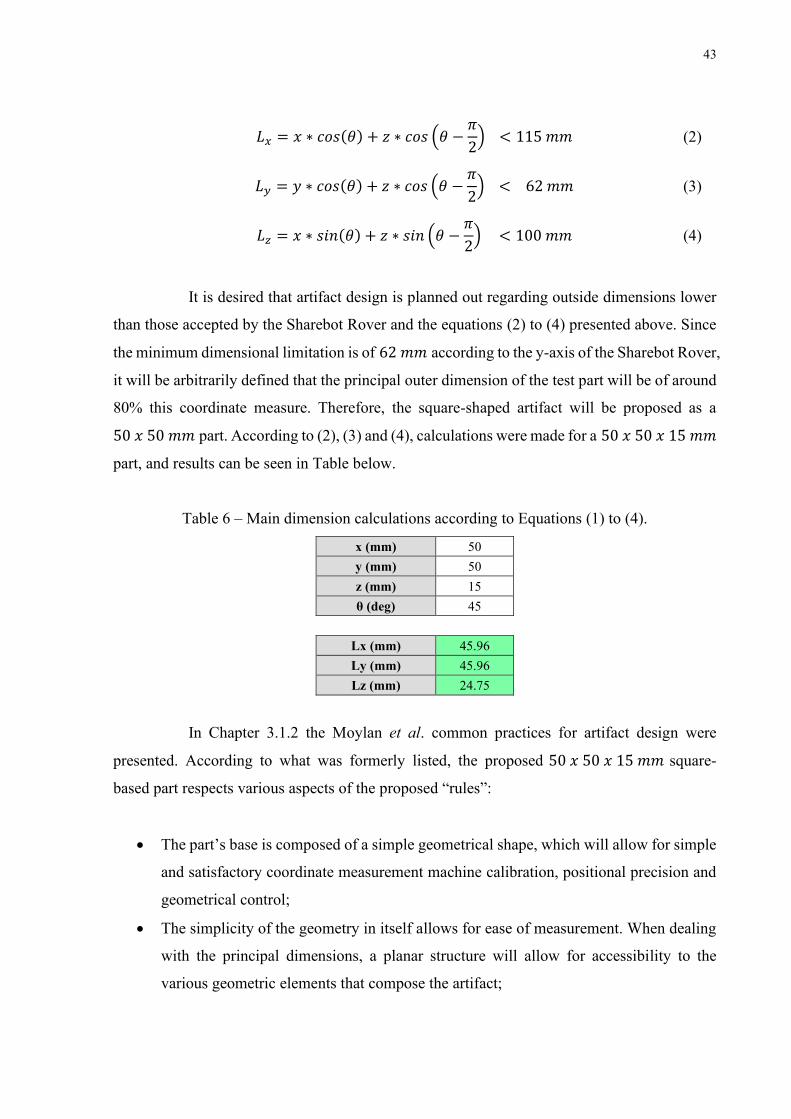
It is desired that artifact design is planned out regarding outside dimensions lower

than those accepted by the Sharebot Rover and the equations (2) to (4) presented above. Since

the minimum dimensional limitation is of 62 𝑚𝑚 according to the y-axis of the Sharebot Rover,

it will be arbitrarily defined that the principal outer dimension of the test part will be of around

80% this coordinate measure. Therefore, the square-shaped artifact will be proposed as a

50 𝑥 50 𝑚𝑚 part. According to (2), (3) and (4), calculations were made for a 50 𝑥 50 𝑥 15 𝑚𝑚

part, and results can be seen in Table below.

Table 6 – Main dimension calculations according to Equations (1) to (4).

x (mm) 50 y (mm) 50 z (mm) 15 θ (deg) 45

Lx (mm) 45.96 Ly (mm) 45.96 Lz (mm) 24.75

In Chapter 3.1.2 the Moylan et al. common practices for artifact design were

presented. According to what was formerly listed, the proposed 50 𝑥 50 𝑥 15 𝑚𝑚 square-

based part respects various aspects of the proposed “rules”:

• The part’s base is composed of a simple geometrical shape, which will allow for simple

and satisfactory coordinate measurement machine calibration, positional precision and

geometrical control;

• The simplicity of the geometry in itself allows for ease of measurement. When dealing

with the principal dimensions, a planar structure will allow for accessibility to the

various geometric elements that compose the artifact;

44

• Despite the fact that all machines allow larger artifacts in the z-axis (as seen in Eq. (4)),

the design proposes a height of only 15 𝑚𝑚, which will preserve the artifact’s small

sizing, allowing for faster build times and low consumption of material.

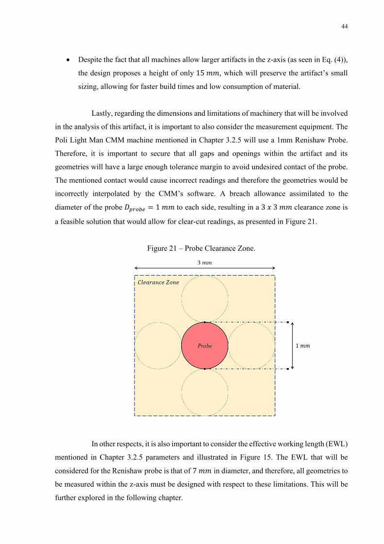
Lastly, regarding the dimensions and limitations of machinery that will be involved

in the analysis of this artifact, it is important to also consider the measurement equipment. The

Poli Light Man CMM machine mentioned in Chapter 3.2.5 will use a 1mm Renishaw Probe.

Therefore, it is important to secure that all gaps and openings within the artifact and its

geometries will have a large enough tolerance margin to avoid undesired contact of the probe.

The mentioned contact would cause incorrect readings and therefore the geometries would be

incorrectly interpolated by the CMM’s software. A breach allowance assimilated to the

diameter of the probe 𝐷𝑝𝑟𝑜𝑏𝑒 = 1 𝑚𝑚 to each side, resulting in a 3 𝑥 3 𝑚𝑚 clearance zone is

a feasible solution that would allow for clear-cut readings, as presented in Figure 21.

Figure 21 – Probe Clearance Zone.

In other respects, it is also important to consider the effective working length (EWL)

mentioned in Chapter 3.2.5 parameters and illustrated in Figure 15. The EWL that will be

considered for the Renishaw probe is that of 7 𝑚𝑚 in diameter, and therefore, all geometries to

be measured within the z-axis must be designed with respect to these limitations. This will be

further explored in the following chapter.

45

3.3.2 Selected Geometries

The type of study at hand is a geometric benchmark, and regarding this category of

analysis, it is essential that the test artifact contains various classic geometries from which form

error and geometric tolerances are derived. Amidst the geometries presented in Table 5, classic

configurations (planes, cylinders, cones, spheres, prismatic features) will be included as both

positive (embossed, or “boss” parts) or negatives (hollow and convex elements; holes) as a way

of optimizing the available area of the artifact. Table 7 specifies the chosen geometries that

have been chosen and will be observed throughout this section. A detailed approach to each

geometries subcategory and label can be found in APPENDIX A – at the end of this document.

Table 7 – Geometry listing of the proposed test part.

ID Family A Concentric Cylinder Boss B Cylinder Boss C Pins D Hemispheres E Circular Holes F Square Boss G Horizontal Cylinders H Staircases I Inclines J Rectangular Boss K Cone L Outer Dimensions M Square Notches

3.3.2.1 Concentric Cylinder Boss – Family A

Concentric cylinder boss is a hollow cylindric feature family that is composed of

two coaxial cylinders, labeled as A1 and A2, where their diameters are of 20 mm and 15 mm,

respectively. The height of feature A2 is of 10 mm from the base, and A1 is only 5 mm from

the same reference – therefore, from the annular plane formed on A1, A2 is only 5 mm higher.

Both contain a hollow region, or a “punched hole” that passes the base of the part, forming the

larger circular hole of the feature family E. This feature will be utilized in order to evaluate

cylindricity, concentricity, circularity, flatness and a general overview of IT grades in each

machine.

46

Figure 22 – Visual representation of the artifact highlighting the feature family A.

3.3.2.2 Cylinder Boss – Family B

Cylinder boss is a solid cylindric feature family that is composed of three separate

cylinders, labeled as B1, B2 and B3, where their diameters are of 2 mm, 3 mm, and 4 mm,

respectively. The height of all features is 3 mm, and they are located between the Rectangular

boss and Pins features. This feature will be utilized in order to evaluate cylindricity, flatness

and a general overview of IT grades for heights in each machine.

Figure 23 – Visual representation of the artifact highlighting the feature family B.

3.3.2.3 Pins – Family C

The Pins are a cylindric feature family that is composed of three separate holes or

“hollow” cylinders, labeled as C1, C2 and C3, where their diameters are of 2 mm, 3 mm, and 4

mm, respectively. The height of all features is 3 mm, and they are located between the

Rectangular boss and Cylinder boss features. This feature will be utilized in order to evaluate

cylindricity and a general overview of IT grades for heights in each machine.

47

Figure 24 – Visual representation of the artifact highlighting the feature family C.

3.3.2.4 Hemisphere – Family D

The Hemisphere feature family is the representation of a half-sphere in both a positive

(convex) and negative (concave) portrayal of the same size, making each feature effectively a

quarter-sphere. The negative rendering of the feature is labeled as D1, whilst the positive

version is D2. Both spherical features have a nominal diameter of 8 mm. This feature will be

utilized in order to evaluate precision in the fabrication of spherical elements and a general

overview of IT grades in each machine.

Figure 25 – Visual representation of the artifact highlighting the feature family D.

3.3.2.5 Circular Holes – Family E

The Circular Holes are a cylindric feature family that is composed of four separate

passing holes onto the artifact base, labeled from E1 to E4 in crescent order. The diameters of

each hole are of 3 mm, 5 mm, and 7 mm and 10mm from E1 through E4, in order. This feature

will be utilized in order to evaluate cylindricity, circularity, concentricity, and a general

overview of IT grades for heights in each machine.

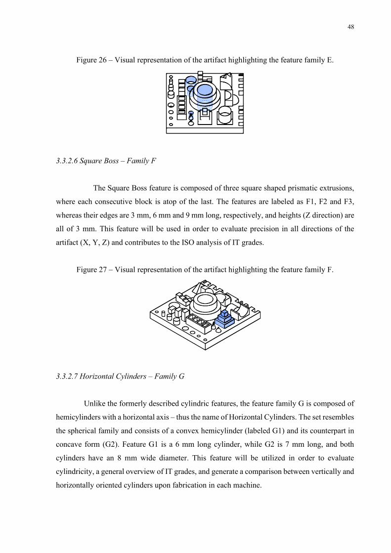
48

Figure 26 – Visual representation of the artifact highlighting the feature family E.

3.3.2.6 Square Boss – Family F

The Square Boss feature is composed of three square shaped prismatic extrusions,

where each consecutive block is atop of the last. The features are labeled as F1, F2 and F3,

whereas their edges are 3 mm, 6 mm and 9 mm long, respectively, and heights (Z direction) are

all of 3 mm. This feature will be used in order to evaluate precision in all directions of the

artifact (X, Y, Z) and contributes to the ISO analysis of IT grades.

Figure 27 – Visual representation of the artifact highlighting the feature family F.

3.3.2.7 Horizontal Cylinders – Family G

Unlike the formerly described cylindric features, the feature family G is composed of

hemicylinders with a horizontal axis – thus the name of Horizontal Cylinders. The set resembles

the spherical family and consists of a convex hemicylinder (labeled G1) and its counterpart in

concave form (G2). Feature G1 is a 6 mm long cylinder, while G2 is 7 mm long, and both

cylinders have an 8 mm wide diameter. This feature will be utilized in order to evaluate

cylindricity, a general overview of IT grades, and generate a comparison between vertically and

horizontally oriented cylinders upon fabrication in each machine.

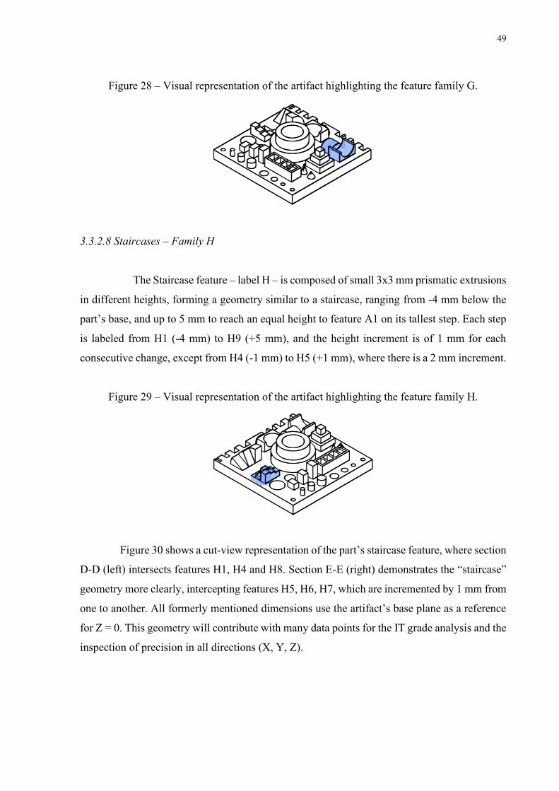
49

Figure 28 – Visual representation of the artifact highlighting the feature family G.

3.3.2.8 Staircases – Family H

The Staircase feature – label H – is composed of small 3x3 mm prismatic extrusions

in different heights, forming a geometry similar to a staircase, ranging from -4 mm below the

part’s base, and up to 5 mm to reach an equal height to feature A1 on its tallest step. Each step

is labeled from H1 (-4 mm) to H9 (+5 mm), and the height increment is of 1 mm for each

consecutive change, except from H4 (-1 mm) to H5 (+1 mm), where there is a 2 mm increment.

Figure 29 – Visual representation of the artifact highlighting the feature family H.

Figure 30 shows a cut-view representation of the part’s staircase feature, where section

D-D (left) intersects features H1, H4 and H8. Section E-E (right) demonstrates the “staircase”

geometry more clearly, intercepting features H5, H6, H7, which are incremented by 1 mm from

one to another. All formerly mentioned dimensions use the artifact’s base plane as a reference

for Z = 0. This geometry will contribute with many data points for the IT grade analysis and the

inspection of precision in all directions (X, Y, Z).

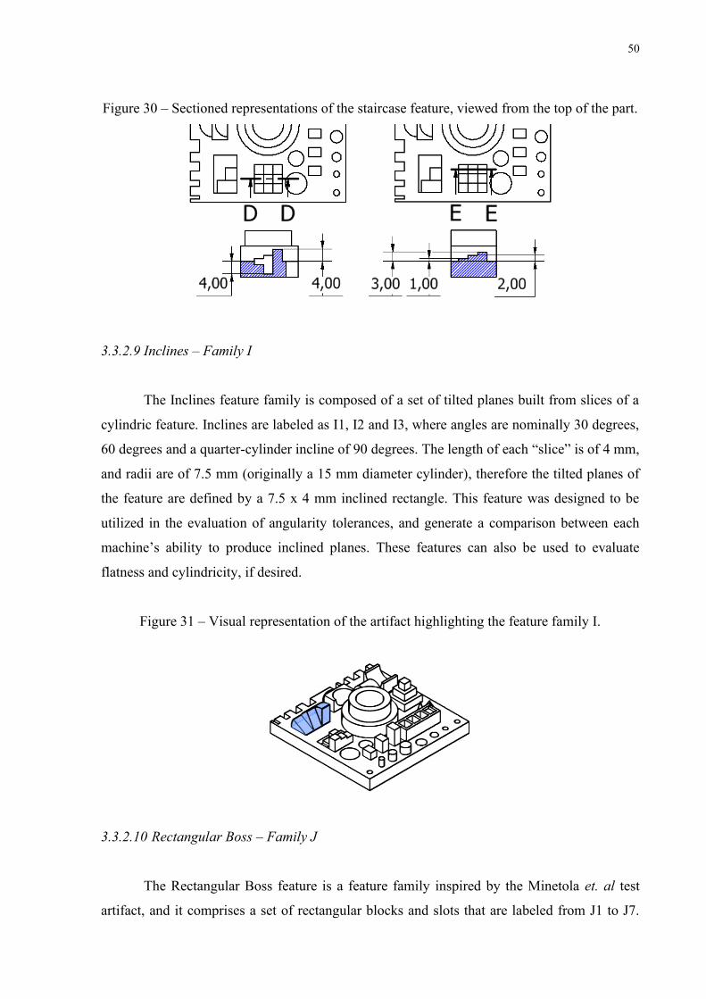
50

Figure 30 – Sectioned representations of the staircase feature, viewed from the top of the part.

3.3.2.9 Inclines – Family I

The Inclines feature family is composed of a set of tilted planes built from slices of a

cylindric feature. Inclines are labeled as I1, I2 and I3, where angles are nominally 30 degrees,

60 degrees and a quarter-cylinder incline of 90 degrees. The length of each “slice” is of 4 mm,

and radii are of 7.5 mm (originally a 15 mm diameter cylinder), therefore the tilted planes of

the feature are defined by a 7.5 x 4 mm inclined rectangle. This feature was designed to be

utilized in the evaluation of angularity tolerances, and generate a comparison between each

machine’s ability to produce inclined planes. These features can also be used to evaluate

flatness and cylindricity, if desired.

Figure 31 – Visual representation of the artifact highlighting the feature family I.

3.3.2.10 Rectangular Boss – Family J

The Rectangular Boss feature is a feature family inspired by the Minetola et. al test

artifact, and it comprises a set of rectangular blocks and slots that are labeled from J1 to J7.

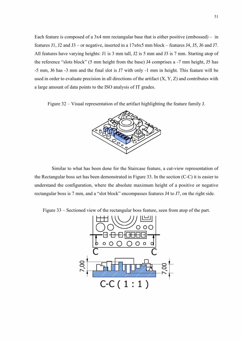
51

Each feature is composed of a 3x4 mm rectangular base that is either positive (embossed) – in

features J1, J2 and J3 – or negative, inserted in a 17x6x5 mm block – features J4, J5, J6 and J7.

All features have varying heights: J1 is 3 mm tall, J2 is 5 mm and J3 is 7 mm. Starting atop of

the reference “slots block” (5 mm height from the base) J4 comprises a -7 mm height, J5 has

-5 mm, J6 has -3 mm and the final slot is J7 with only -1 mm in height. This feature will be

used in order to evaluate precision in all directions of the artifact (X, Y, Z) and contributes with

a large amount of data points to the ISO analysis of IT grades.

Figure 32 – Visual representation of the artifact highlighting the feature family J.

Similar to what has been done for the Staircase feature, a cut-view representation of

the Rectangular boss set has been demonstrated in Figure 33. In the section (C-C) it is easier to

understand the configuration, where the absolute maximum height of a positive or negative

rectangular boss is 7 mm, and a “slot block” encompasses features J4 to J7, on the right side.

Figure 33 – Sectioned view of the rectangular boss feature, seen from atop of the part.

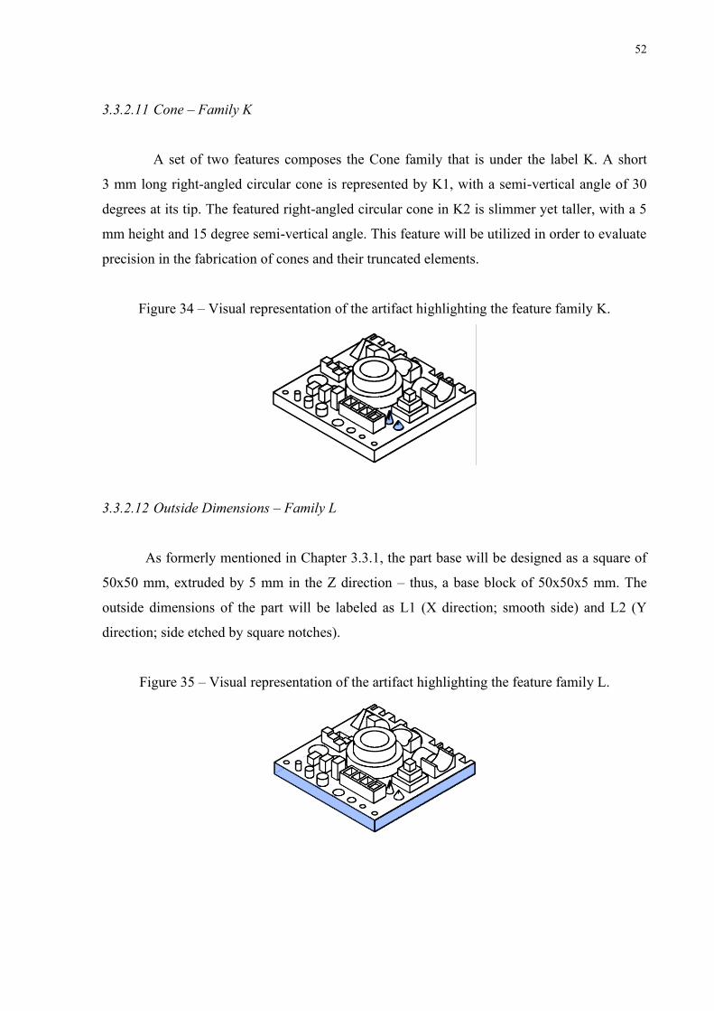
52

3.3.2.11 Cone – Family K

A set of two features composes the Cone family that is under the label K. A short

3 mm long right-angled circular cone is represented by K1, with a semi-vertical angle of 30

degrees at its tip. The featured right-angled circular cone in K2 is slimmer yet taller, with a 5

mm height and 15 degree semi-vertical angle. This feature will be utilized in order to evaluate

precision in the fabrication of cones and their truncated elements.

Figure 34 – Visual representation of the artifact highlighting the feature family K.

3.3.2.12 Outside Dimensions – Family L

As formerly mentioned in Chapter 3.3.1, the part base will be designed as a square of

50x50 mm, extruded by 5 mm in the Z direction – thus, a base block of 50x50x5 mm. The

outside dimensions of the part will be labeled as L1 (X direction; smooth side) and L2 (Y

direction; side etched by square notches).

Figure 35 – Visual representation of the artifact highlighting the feature family L.

53

3.3.2.13 Square Notches – Family M

The Square notch feature is composed of 3x3 mm square-shaped indentations made

onto one of the faces of the base. As per Figure 36, the right-sided notches are rendered square

by irregular etches on the part, whilst the left-sided notches are even square-shaped etches

engraved on the part. Features are labeled M1 to M7, from right to left. This feature will be

used in order to evaluate the accuracy of edge-imprinted features in each machine, as well as to

generate a large amount of data points for the ISO IT grade analysis.

Figure 36 – Visual representation of the artifact highlighting the feature family M.

3.3.3 Analyzed Derivative Characteristics

A process planning study by Lynn-Charney et al. [47] in the field of accuracy models

for manufacturing states tolerance, surface and orientation relationships between different types

of geometries and the derivative characteristics that each one will produce – such as

concentricity, positioning, circularity, etc. The affiliation of a geometry to a part’s physical

characteristics was initially detailed in Chapter 3.2.6.6 and the listing in Table 8 below states

the chosen features to evaluate secondary, derivative aspects of the test part.

Table 8 – Derivative characteristic listing of the proposed test part

ID Family N Vertical Cylinders O Concentricity P Planes

54

3.3.3.1 Concentricity and Vertical Cylinders – Family N and O

For measurement and analysis purposes a group of four features will be used to

evaluate concentricity. All features used are fundamentally vertical cylinders, and the features

selected are A1 and A2 from Concentric Cylinder Boss, B3 from Cylinder Boss, and E4 the

Circular Hole located in the middle of the part. All features will be measured once again and

labeled as “Vertical Cylinders” under the letter “N”, and concentricity data will be labeled “O”.

Only features A1, A2 and E4 will be used for concentricity, and the label of each combination

can be found in APPENDIX A – Geometric Labeling (Figure 85).

Figure 37 – Visual representation of the features that compose families N and O.

3.3.3.2 Horizontal Planar Surfaces of Interest – Family P

In order to evaluate flatness, parallelism, and surface irregularities it is necessary to

define which planes will compose the measurement data. A set of 10 horizontal planes was

selected for the evaluation of these characteristics, and Table 9 catalogues the selection by the

feature from which the plane is originated.

Figure 38 – Visual representation of the artifact highlighting the planes selected for family P.

55

Table 9 – Detailed description of the selection of planes for feature family P.

ID Related Feature Description

P1 - Plane of the base P2 A1 Concentric cylinder boss P3 A2 Concentric cylinder boss P4 H7 Square step on Staircases P5 H8 Square step on Staircases P6 H9 Square step on Staircases P7 F2 Superior plane of square boss feature P8 F3 Superior plane of square boss feature P9 B3 Cylinder boss feature

P10 J(-) Superior face of the negative slot block

4. EXPERIMENTAL DEVELOPMENT

The experimental analysis explored within this chapter will cover both an overview

of the experimental procedures, methodology and its conjectural background information. This

material will deal with machine setup, instructions and the series of procedures taken in order

to fabricate the replicas of the defined artifact part. On each of the compared machines, a single

replica of the artifact part was manufactured using the same STL file that was designed

throughout Chapter 3. Each machine had a specific slicing software that was used to prepare

the numerical control file for printing.

4.1 Preparation procedures

The preparation of the additive manufacturing processes can be divided into two

categories: 3D model preparing and machine setup. The first segment refers to the processing

and conversion of the 3D CAD model into an adequate file format. When dealing with 3D

systems, most models are likely to be produced in .STL or .OBJ formats. The artifact used in

this study was initially produced in Autodesk Inventor (.IPT CAD format) and converted

to .STL after the inclusion of supporting structures using CIMsystem’s Pyramis 3D printing

management software [48]. Furthermore, the STL file can be sliced with freeware slicing

software or the machine manufacturer’s own package, and the print path is converted into a

standard ISO G-code file. This denotes that the machine will promptly be able to attain the file

(via ethernet or USB) with instructions regarding position and orientation of the part, which

will allow the commencement of fabrication.

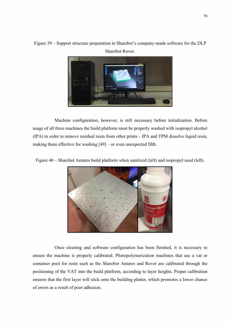
56

Figure 39 – Support structure preparation in Sharebot’s company-made software for the DLP

Sharebot Rover.

Machine configuration, however, is still necessary before initialization. Before

usage of all three machines the build platform must be properly washed with isopropyl alcohol

(IPA) in order to remove residual resin from other prints – IPA and TPM dissolve liquid resin,

making them effective for washing [49] – or even unexpected filth.

Figure 40 – Sharebot Antares build platform when sanitized (left) and isopropyl used (left).

Once cleaning and software configuration has been finished, it is necessary to

ensure the machine is properly calibrated. Photopolymerization machines that use a vat or

container pool for resin such as the Sharebot Antares and Rover are calibrated through the

positioning of the VAT into the build platform, according to layer heights. Proper calibration

ensures that the first layer will stick onto the building platter, which promotes a lower chance

of errors as a result of poor adhesion.

57

4.2 Fabrication of the replicas

As soon as preparation is finished, it is possible to initialize the machine and begin

fabrication. The beginning of the manufacturing processes is generally slower, since layers that

are produced first generally encompass a larger surface area, which results in a longer build-

time for initial layers of the base, brims, rafts, and supports.

In this chapter the fabrication procedures and post-processing steps for the parts

will be approached in each machine. Initially, both Sharebot machines will be analyzed since

the stages of fabrication in SLA and DLP are remarkably similar, as these are naturally

resemblant additive manufacturing processes. Afterwards, the more straightforward procedures

of the Objet30 will be described for assessment of all manufacturing processes.

4.2.1 Sharebot Rover and Antares – Fabrication description and detail

Sharebot machines comprise VAT Photopolymerization processes, in which resin

must be placed into the container in which the build platform will be submerged. The first part

that was manufactured was the DLP replica on the Sharebot Rover. It is recommended that the

entirety of the resin tank is filled for manufacturing, and around 18g of resin were consumed

for each part. The resin used in DLP was the Sharebot S-Clear and the part was fabricated in

approximately 16 hours with a layer thickness of 50 microns (initial estimates of the machine

indicated a total of 14 hours, as seen in Figure 41). The resin costs 199.00 €/kg, which would

indicate that the part had a cost of roughly 3.60 €, discounting occasional resin losses from

filling the container [50]. A summary containing details about the S-Clear resin and its

proprieties will be contained in “APPENDIX B – Summary of Resins”.

Figure 41 – Printing initialization of the Sharebot Rover for the DLP replica.

58

Figure 42 – DLP test part after printing completion.

Both DLP and SLA parts were printed in a 45 degree angle, and column supports were

utilized (Figure 42). Once manufacturing is complete, the part must be scraped from the build

platform and delicacy is not mandatory since the elements that are in contact with the platform

are disposable (supports and skirts; Figure 42). Since post-fabrication procedures are similar

for all parts produced, this content will be presented in Chapter 4.2.3.

Figure 43 – Removal of the DLP part from the printing platform.

The stereolithography (SLA) part produced in the Sharebot Antares used another resin,

the Sharebot PR-S high precision resin. Differently from the DLP resin, which was transparent,

this photopolymer used in SLA is grey, with layer thickness of 50 microns and took roughly 4

hours to fabricate the reference part (considerably faster than the Sharebot Rover). The resin

costs 149.00 €/kg, therefore, discounting eventual losses, the material price for manufacturing

one test part is of around 2.80 € [51]. The Sharebot Antares uses an individual 3D management

supporting and slicing software, and parts are transferred via an Ethernet connection. Further

details about the material will be described in APPENDIX B – Summary of Resins.

59

Figure 44 – Sharebot Antares open for initialization.

Figure 45 – Close-up photo of the Sharebot Antares during fabrication.

In Figure 45 a visual depiction of the main difference between SLA and DLP can be

seen. On the bottom left corner of the image it is possible to notice the position in which the

UV laser is curing the current layer of the part. The main difference between a DLP process

and SLA is the operation of the light source; SLA uses a single UV laser, while the DLP

machine uses light that is projected from a stationary source. In DLP, light source cures the

complete layer of resin once at a time, while in SLA, the laser moves around the build platform,

tracing the part’s geometry [52]. After completion, both parts were successfully removed and

prepared for their respective post-fabrication procedures.

4.2.2 Stratasys Objet30 – Fabrication description and detail

Fabrication of PolyJet on the Stratasys Objet30 was a much simpler procedure, where

the machine’s proper 3D management software is available and capable of qualitatively

delivering a support structure and sliced layers of the STL file. Importing was also performed

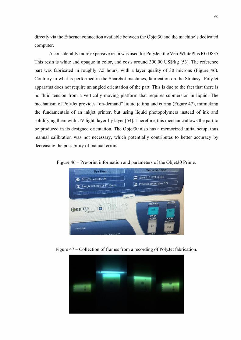
60

directly via the Ethernet connection available between the Objet30 and the machine’s dedicated

computer.

A considerably more expensive resin was used for PolyJet: the VeroWhitePlus RGD835.

This resin is white and opaque in color, and costs around 300.00 US$/kg [53]. The reference

part was fabricated in roughly 7.5 hours, with a layer quality of 30 microns (Figure 46).

Contrary to what is performed in the Sharebot machines, fabrication on the Stratasys PolyJet

apparatus does not require an angled orientation of the part. This is due to the fact that there is

no fluid tension from a vertically moving platform that requires submersion in liquid. The

mechanism of PolyJet provides “on-demand” liquid jetting and curing (Figure 47), mimicking

the fundamentals of an inkjet printer, but using liquid photopolymers instead of ink and

solidifying them with UV light, layer-by layer [54]. Therefore, this mechanic allows the part to

be produced in its designed orientation. The Objet30 also has a memorized initial setup, thus

manual calibration was not necessary, which potentially contributes to better accuracy by

decreasing the possibility of manual errors.

Figure 46 – Pre-print information and parameters of the Objet30 Prime.

Figure 47 – Collection of frames from a recording of PolyJet fabrication.

61

4.2.3 Post-fabrication of the parts produced

Post processing in all of the manufacturing procedures presented thus far are

composed of two possible steps: ultrasonic cleaning or washing; and UV curing. The first step

after the removal of the part from the machine it to wash the part properly, in order to remove

any residual liquid resin. Hence, the use of a solution such as the Isopropyl Alcohol (IPA) is

once again necessary. For the Sharebot machine’s reference parts, each artifact was placed in

an ultrasonic bath.

A Digital Ultrasonic Cleaner (DUC) is a machine that uses vibration, fluid

proprieties and heating to perform final conditioning of a resin-based AM part. In its interior,

IPA is used in order to dissolve any lingering resin on the part. The heating effect was not

available at RMLAB’s DUC, therefore the ultrasonic bath was based only on wave emission

and submerging the SLA and DLP parts, individually, in Isopropyl.

Figure 48 – Sharebot Digital Ultrasonic Cleaner.

Source: [55]

Furthermore, the second part of post-processing in the SLA and DLP procedures is

the usage of a UV chamber or oven. As described by Sharebot, post-curing is a process that

aims to stabilize a resin 3D model after printing, and to complete polymerization [55]. This

ensures that the hardened models retain their structural characteristics and a uniform yield. Post-

curing, however, can be done within a UV chamber or even through alternative methods such

as exposure to sunlight. The Sharebot UV Curing Box (UCB) was used for curing of the SLA

and DLP parts for 20 minutes each right after they were fabricated and thoroughly cleaned. A

consumption of about 70W is used to power LED’s of around 375 nm wavelength emissions.

62

Figure 49 – Sharebot UV Curing Box used in this study.

Source: [55]

Figure 50 – DLP (left) and SLA (right) fabricated parts while post-curing inside the UCB.

Finally, it is important to note that the replicas were not finished or polished, in

order to not to alter their surfaces or dimensions. The manufactured condition should be

considered for an accurate benchmarking of the AM machines. This is reinforced in the good-

practices for artifact design of Moylan et. al [17], where it is recommended that the design does

not require much post-processing, in order to preserve the fidelity of the manufacturing results

for the model.

The procedures required for PolyJet were much simpler and faster than those

realized in DLP and SLA. Parts produced by the Objet30 Prime also do not require any post-

processing other than water jetting for washing and a following pressurized air drying (see

Appendix C).

63

4.2.4 Finished parts and expected results

In this chapter a general overview and comparison of the manufacturing processes

will be described. Additionally, general commentary and first impressions of the fabricated

reference parts will be registered.

The first part was produced with the Sharebot Rover, and it was noticeable that the

process took a particularly long time to manufacture the test artifact (16 hours). The machine

requires manual intervention in calibration, and it is difficult to ensure layer adhesion in the

early stages of fabrication. Within the first hour of initialization it is also not possible to

discriminate whether or not the first print layers have attached themselves to the build platform.

At first glance, the part seems well produced and finished, with well-defined basic features

(squares, circles, cylinders etc.) to the naked eye. Conversely, it is also noticeable how the part

seems to have retained and cured resin within some small openings, which will certainly

contribute to inaccuracies regarding the CAD model. Overall, the part is visually satisfactory,

and all geometries seem to have been well produced in the DLP machine.

Figure 51 – Photo of the DLP reference part produced in the Sharebot Rover.

In the second manufacturing process, the Sharebot Antares was used for fabrication

of the SLA part. The interval of time that was necessary to fabricate the part was the shortest

of all machines (only around 4 hours), which makes it feasible to correct setup errors promptly.

Since calibration is also not automatic in the Antares, it may be challenging to obtain proper

layer adhesion. It is also worth noting that this is a potential source of human error which may

affect the geometric accuracy of the part. To the naked eye, the produced part seems to have

better finishing characteristic than the DLP. However, some localized errors are very clear, such

as a slight one-sided warping under the base, which opportunely is expected to not affect the

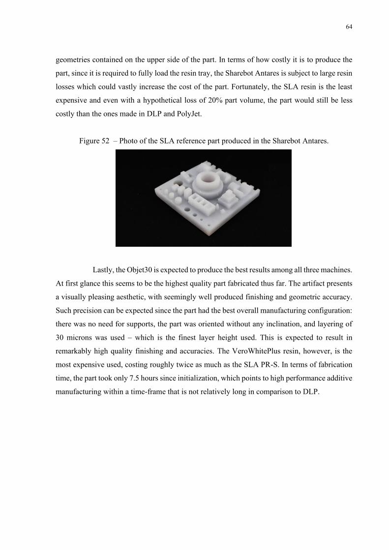
64

geometries contained on the upper side of the part. In terms of how costly it is to produce the

part, since it is required to fully load the resin tray, the Sharebot Antares is subject to large resin

losses which could vastly increase the cost of the part. Fortunately, the SLA resin is the least

expensive and even with a hypothetical loss of 20% part volume, the part would still be less

costly than the ones made in DLP and PolyJet.

Figure 52 – Photo of the SLA reference part produced in the Sharebot Antares.

Lastly, the Objet30 is expected to produce the best results among all three machines.

At first glance this seems to be the highest quality part fabricated thus far. The artifact presents

a visually pleasing aesthetic, with seemingly well produced finishing and geometric accuracy.

Such precision can be expected since the part had the best overall manufacturing configuration:

there was no need for supports, the part was oriented without any inclination, and layering of

30 microns was used – which is the finest layer height used. This is expected to result in

remarkably high quality finishing and accuracies. The VeroWhitePlus resin, however, is the

most expensive used, costing roughly twice as much as the SLA PR-S. In terms of fabrication

time, the part took only 7.5 hours since initialization, which points to high performance additive

manufacturing within a time-frame that is not relatively long in comparison to DLP.

65

Figure 53 – Photo of the PolyJet reference part produced in the Stratasys Objet30.

Figure 54 – Side by side photo of all three manufactured reference parts: DLP (left), SLA

(middle) and PolyJet (right).

4.3 Measurement procedure of the replicas

The measurement procedure was conducted in the Poli Light Man coordinate

measurement machine, as formerly mentioned in Chapter 3.2.5. In this chapter, the procedures

and proper measurement practices of a benchmarking part will be described. The literature used

for measurement instructions was the GEOSOFT Manual (“Manuale di utilizzo”) available at

Politecnico di Torino’s RMLAB [56]. Further guidelines were presented in David Flack’s Good

Practice Guide for CMM Measurements [24]. The measurement capabilities and methodology

presented in this document will follow the requirements of the Poli 3D GEOSOFT

Measurement Software of the Poli Light Man.

66

4.3.1 Positioning and Fixation

When setting up the machine, the part must be placed in the Poli Light Man’s

measurement area. In order to the stability of the part, attribute height – a for ease of

measurement – and position the part within a fixed reference position, a mechanical vise (or

fixtures) is used to hold the measured part. When using fixtures it is necessary to ensure that

they are clean, the workpiece is located correctly, clamping forces on the workpiece are not

excessive, and that all features requiring measurement are accessible. In this case, the reference

parts were placed atop of metal placeholders with its base parallel to the granite measurement

board of the Poli Light Man, as indicated in Figure 55. In this setup, the workpiece is not over-

constrained and all geometries are accessible.

Figure 55 – Positioning and fixation of a reference part on the Poli Light Man CMM.

4.3.2 Measurement strategy for standard geometries

The workpiece at hand is composed of various different basic geometries, such as

planes, holes, cylinders, squares, rectangles, cones, spheres etc. Mathematically, each geometry

has a minimum amount of points (or data values) required to execute fitting of a geometric

feature. The minimum number of contact points required for each type of feature to be measured

and fitted is presented in Table 10 below, from David Flack’s good practices guide.

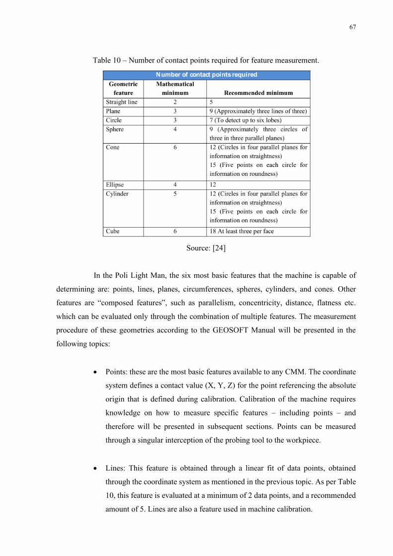
67

Table 10 – Number of contact points required for feature measurement.

Source: [24]

In the Poli Light Man, the six most basic features that the machine is capable of

determining are: points, lines, planes, circumferences, spheres, cylinders, and cones. Other

features are “composed features”, such as parallelism, concentricity, distance, flatness etc.

which can be evaluated only through the combination of multiple features. The measurement

procedure of these geometries according to the GEOSOFT Manual will be presented in the

following topics:

• Points: these are the most basic features available to any CMM. The coordinate

system defines a contact value (X, Y, Z) for the point referencing the absolute

origin that is defined during calibration. Calibration of the machine requires

knowledge on how to measure specific features – including points – and

therefore will be presented in subsequent sections. Points can be measured

through a singular interception of the probing tool to the workpiece.

• Lines: This feature is obtained through a linear fit of data points, obtained

through the coordinate system as mentioned in the previous topic. As per Table

10, this feature is evaluated at a minimum of 2 data points, and a recommended

amount of 5. Lines are also a feature used in machine calibration.

68

• Planes: a planar feature can be defined through a minimum of three points, and

in this work a minimum of 9 points will be used for small area finite planes. The

Planes feature (“P” label; P1-P10) will be evaluated under these conditions,

where small 3x3 mm planes such as P4-P6 will be sampled in 9 points, and

other planes such as P1 may contain up to 30 data points (maximum collection

of data points allowed in the Poli Light Man for a single measurement). Unlike

the previous two features, a plane will return a mean deviation of its

measurement (𝛿) and a maximum deviation observed (𝑆𝑚𝑎𝑥).

• Circumferences: circular features and diameters can be evaluated through this

feature in order to interpolate a circle that would fit through a minimum of 3

data points. It is recommended that this feature is measured with at least 7 points,

and deviations such as those mentioned for planes are an output of this feature,

such as all features that contain a minimum of at least 3 data points.

• Spheres: this feature will be used exclusively for the measurement of the

Hemisphere set of the reference part (feature “D”). The sphere is the non-planar

feature that can be evaluated in the CMM thus far, and it requires a minimum

of 4 points in order to define a fitting combination of circumferences. A

minimum of 6 points is recommended by the GEOSOFT manual, whereas

David Flack’s manual suggests a more conservative approach of 9 data points.

The GEOSOFT manual recommends that data points are measured in groups of

three, where each group is contained at an equal latitude (or sectional diameter)

of the sphere, as illustrated by Figure 56.

Figure 56 – Recommended distribution of data points on a sphere.

Source: [24]

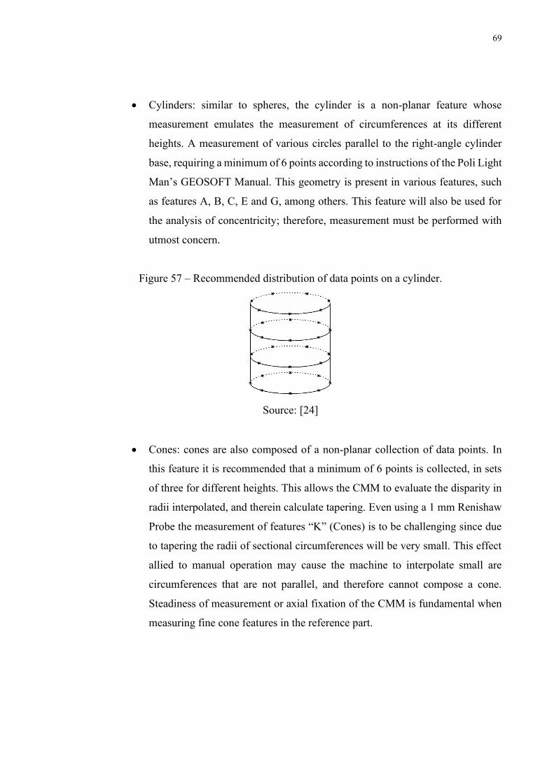
69

• Cylinders: similar to spheres, the cylinder is a non-planar feature whose

measurement emulates the measurement of circumferences at its different

heights. A measurement of various circles parallel to the right-angle cylinder

base, requiring a minimum of 6 points according to instructions of the Poli Light

Man’s GEOSOFT Manual. This geometry is present in various features, such

as features A, B, C, E and G, among others. This feature will also be used for

the analysis of concentricity; therefore, measurement must be performed with

utmost concern.

Figure 57 – Recommended distribution of data points on a cylinder.

Source: [24]

• Cones: cones are also composed of a non-planar collection of data points. In

this feature it is recommended that a minimum of 6 points is collected, in sets

of three for different heights. This allows the CMM to evaluate the disparity in

radii interpolated, and therein calculate tapering. Even using a 1 mm Renishaw

Probe the measurement of features “K” (Cones) is to be challenging since due

to tapering the radii of sectional circumferences will be very small. This effect

allied to manual operation may cause the machine to interpolate small are

circumferences that are not parallel, and therefore cannot compose a cone.

Steadiness of measurement or axial fixation of the CMM is fundamental when

measuring fine cone features in the reference part.

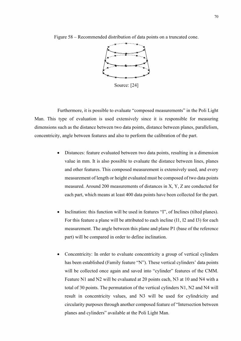
70

Figure 58 – Recommended distribution of data points on a truncated cone.

Source: [24]

Furthermore, it is possible to evaluate “composed measurements” in the Poli Light

Man. This type of evaluation is used extensively since it is responsible for measuring

dimensions such as the distance between two data points, distance between planes, parallelism,

concentricity, angle between features and also to perform the calibration of the part.

• Distances: feature evaluated between two data points, resulting in a dimension

value in mm. It is also possible to evaluate the distance between lines, planes

and other features. This composed measurement is extensively used, and every

measurement of length or height evaluated must be composed of two data points

measured. Around 200 measurements of distances in X, Y, Z are conducted for

each part, which means at least 400 data points have been collected for the part.

• Inclination: this function will be used in features “I”, of Inclines (tilted planes).

For this feature a plane will be attributed to each incline (I1, I2 and I3) for each

measurement. The angle between this plane and plane P1 (base of the reference

part) will be compared in order to define inclination.

• Concentricity: In order to evaluate concentricity a group of vertical cylinders

has been established (Family feature “N”). These vertical cylinders’ data points

will be collected once again and saved into “cylinder” features of the CMM.

Feature N1 and N2 will be evaluated at 20 points each, N3 at 10 and N4 with a

total of 30 points. The permutation of the vertical cylinders N1, N2 and N4 will

result in concentricity values, and N3 will be used for cylindricity and

circularity purposes through another composed feature of “Intersection between

planes and cylinders” available at the Poli Light Man.

71

• Parallelism: this can be obtained in two different methods in the Poli Light Man:

composed feature number 14 or number 31. Essentially, the measurement

encompasses the combination of two planes, and once again the feature “P” will

be utilized. Function 14 returns the parallelism as a value in “mm/mt” indicating

how much the interpolated planes distance themselves over a large distance.

Function 31, on the other hand, utilizes an approach similar to what is expected

in ISO standards, where parallelism is defined as a tolerance zone in mm to

which all points of the “non-parallel” plane are contained.

4.3.3 CMM Calibration

In order to calibrate a CMM machine, an understanding of how features are

measured is fundamental. The process of calibration in itself requires the measurement and

definition of a plane, two lines, one point and a sphere.

The first part of CMM setup is the probe’s stylus calibration. This is performed

through the use of a certified reference sphere of qualification. During this phase, the CMM

will prompt the user to indicate which qualification sphere is being used, and the probe stylus

should be driven perpendicularly to the sphere in several directions. This allows the CMM to

compensate measurements for effects of pre-travel variation of the touch trigger, which can

induce large errors to measurements [57]. In this analysis, a 16 mm reference sphere was used

for calibration of the 1 mm probe stylus.

Figure 59 - Qualification sphere used in the Poli Light Man.

Once the stylus qualification is performed, it is necessary to define the global

coordinate system (and origin) of the CMM through positioning calibration. In order to do this,

72

the reference part was fixed as formerly mentioned, and the parts superior base was adopted as

the coordinate reference of Z = 0. Subsequently, it is necessary to define the position of both X

and Y axes, and as seen in Figure 60, the dashed line (yellow) and full line (red) can encompass

there axes, respectively. The GEOSOFT program of the Poli Light Man requests a primary

feature, a secondary feature and an origin point. By definition, the primary feature used is the

reference plane (in this case, feature P1). The secondary feature can be either axis formerly

probed as a line-feature – for the sake of choice, assume a selection of the full line (red). Lastly,

the machine requires an origin point that intersects both Z = 0 and Y = 0 in order to define the

last remaining coordinate. The origin point (in green, Figure 60) is obtained as a “composed

feature” of “intersection between two lines”, resulting in the origin required for calibration.

Once this is performed, the machine should identify the green point as [X,Y,Z] = [0,0,0].

Similar to what is seen in Figure 60, the following Figure 61 shows the setup on the actual

reference part. Once calibration is completed, measurements can be succesfully conducted for

analysis.

Figure 60 – Illustration of geometries necessary for part calibration.

Figure 61 – Illustration of geometries necessary for calibration on a real reference part.

73

5. ANALYSIS AND RESULTS

A comparison of the three manufacturing systems described will be conducted

within the following chapters. Initially, the analysis will be carried out within a framework

established by the International Organization for Standardization (ISO) of basic dimensional

ranges. Furthermore, a quality analysis will be realized: the collected data will be processed in

order to evaluate the statistical distribution of measurements realized. Manufacturing results

can therein be presented in terms of the probability of each process’ machine and equipment of

fabricating a qualitatively complying part.

It is important to have references as to which results are expected from the analysis.

In a benchmarking analysis of fused deposition modeling systems (FDM) by Minetola et al.

[58], it is possible to establish a correlation of expected results for additive manufacturing

methods. In that case, however, it is possible to assume that the fused-polymer fabrication

machines would produce less accurate parts than photopolymer UV-curing based processes

such as SLA, DLP and PolyJet. According to Minetola et al., it is anticipated that the relative

accuracy of a machine – established by ISO ranges – would increase as basic sizes increase. In

other words, an additive manufacturing system will generally allow its user to manufacture

smaller features with coarser accuracy, albeit an acceptable deviation for an IT grade not being

constant and changing with the size of the feature by means of the standard tolerance factor,

which will be further elaborated.

5.1 Dimensional accuracy in IT Grades

Every manufacturing process has a quantitative parameter to which its precision is

correlated. According to ISO 286 [59], this value is referred to as an International Tolerance

(IT) Grade. This grade identifies what is the expected tolerance value that a given process can

create within a particular dimensional range. The values of standard tolerance grades for

nominal sizes up to 500 mm are evaluated through the standard tolerance factor 𝑖 that is

expressed in micrometres according to the following formula:

𝑖 = 0.45 ∙ √𝐷

3+ 0.001 ∙ 𝐷 (5)

In equation (5) above, 𝑖 is presented as a function of the parameter 𝐷, which is the

geometric mean of the ISO range of nominal sizes, being 𝐷1 and 𝐷2 its lower and upper limits,

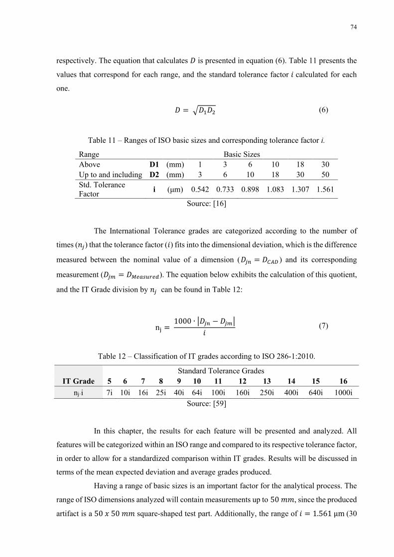
74

respectively. The equation that calculates 𝐷 is presented in equation (6). Table 11 presents the

values that correspond for each range, and the standard tolerance factor 𝑖 calculated for each

one.

𝐷 = √𝐷1𝐷2 (6)

Table 11 – Ranges of ISO basic sizes and corresponding tolerance factor i.

Range Basic Sizes Above D1 (mm) 1 3 6 10 18 30 Up to and including D2 (mm) 3 6 10 18 30 50 Std. Tolerance Factor i (μm) 0.542 0.733 0.898 1.083 1.307 1.561

Source: [16]

The International Tolerance grades are categorized according to the number of

times (𝑛𝑗) that the tolerance factor (𝑖) fits into the dimensional deviation, which is the difference

measured between the nominal value of a dimension (𝐷𝑗𝑛 = 𝐷𝐶𝐴𝐷 ) and its corresponding

measurement (𝐷𝑗𝑚 = 𝐷𝑀𝑒𝑎𝑠𝑢𝑟𝑒𝑑). The equation below exhibits the calculation of this quotient,

and the IT Grade division by 𝑛𝑗 can be found in Table 12:

nj =

1000 ∙ |𝐷𝑗𝑛 − 𝐷𝑗𝑚|

𝑖 (7)

Table 12 – Classification of IT grades according to ISO 286-1:2010.

Standard Tolerance Grades IT Grade 5 6 7 8 9 10 11 12 13 14 15 16

nj·i 7i 10i 16i 25i 40i 64i 100i 160i 250i 400i 640i 1000i Source: [59]

In this chapter, the results for each feature will be presented and analyzed. All

features will be categorized within an ISO range and compared to its respective tolerance factor,

in order to allow for a standardized comparison within IT grades. Results will be discussed in

terms of the mean expected deviation and average grades produced.

Having a range of basic sizes is an important factor for the analytical process. The

range of ISO dimensions analyzed will contain measurements up to 50 𝑚𝑚, since the produced

artifact is a 50 𝑥 50 𝑚𝑚 square-shaped test part. Additionally, the range of 𝑖 = 1.561 μm (30

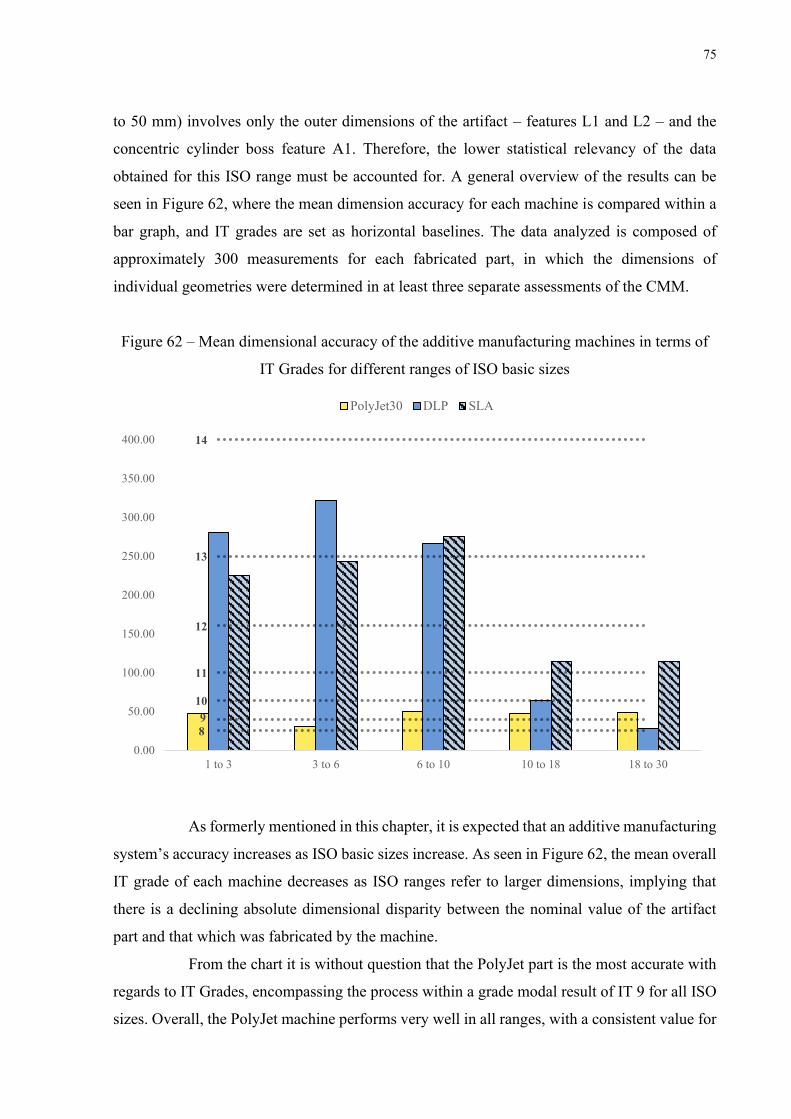
75

to 50 mm) involves only the outer dimensions of the artifact – features L1 and L2 – and the

concentric cylinder boss feature A1. Therefore, the lower statistical relevancy of the data

obtained for this ISO range must be accounted for. A general overview of the results can be

seen in Figure 62, where the mean dimension accuracy for each machine is compared within a

bar graph, and IT grades are set as horizontal baselines. The data analyzed is composed of

approximately 300 measurements for each fabricated part, in which the dimensions of

individual geometries were determined in at least three separate assessments of the CMM.

Figure 62 – Mean dimensional accuracy of the additive manufacturing machines in terms of

IT Grades for different ranges of ISO basic sizes

As formerly mentioned in this chapter, it is expected that an additive manufacturing

system’s accuracy increases as ISO basic sizes increase. As seen in Figure 62, the mean overall

IT grade of each machine decreases as ISO ranges refer to larger dimensions, implying that

there is a declining absolute dimensional disparity between the nominal value of the artifact

part and that which was fabricated by the machine.

From the chart it is without question that the PolyJet part is the most accurate with

regards to IT Grades, encompassing the process within a grade modal result of IT 9 for all ISO

sizes. Overall, the PolyJet machine performs very well in all ranges, with a consistent value for

910

11

12

13

14

80.00

50.00

100.00

150.00

200.00

250.00

300.00

350.00

400.00

1 to 3 3 to 6 6 to 10 10 to 18 18 to 30

PolyJet30 DLP SLA

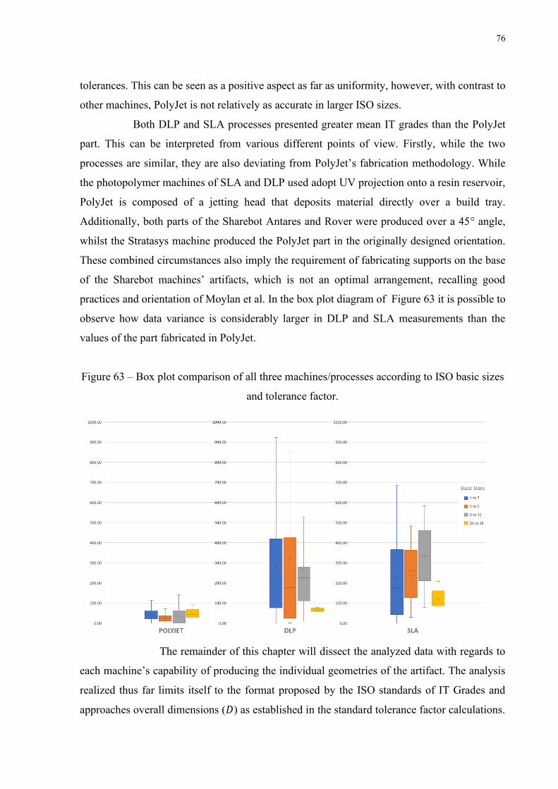
76

tolerances. This can be seen as a positive aspect as far as uniformity, however, with contrast to

other machines, PolyJet is not relatively as accurate in larger ISO sizes.

Both DLP and SLA processes presented greater mean IT grades than the PolyJet

part. This can be interpreted from various different points of view. Firstly, while the two

processes are similar, they are also deviating from PolyJet’s fabrication methodology. While

the photopolymer machines of SLA and DLP used adopt UV projection onto a resin reservoir,

PolyJet is composed of a jetting head that deposits material directly over a build tray.

Additionally, both parts of the Sharebot Antares and Rover were produced over a 45° angle,

whilst the Stratasys machine produced the PolyJet part in the originally designed orientation.

These combined circumstances also imply the requirement of fabricating supports on the base

of the Sharebot machines’ artifacts, which is not an optimal arrangement, recalling good

practices and orientation of Moylan et al. In the box plot diagram of Figure 63 it is possible to

observe how data variance is considerably larger in DLP and SLA measurements than the

values of the part fabricated in PolyJet.

Figure 63 – Box plot comparison of all three machines/processes according to ISO basic sizes

and tolerance factor.

The remainder of this chapter will dissect the analyzed data with regards to

each machine’s capability of producing the individual geometries of the artifact. The analysis

realized thus far limits itself to the format proposed by the ISO standards of IT Grades and

approaches overall dimensions (𝐷) as established in the standard tolerance factor calculations.

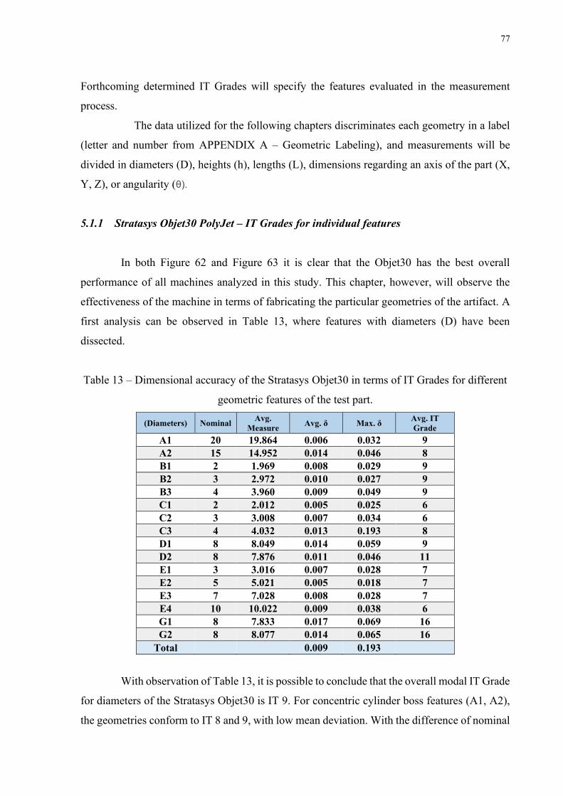
77

Forthcoming determined IT Grades will specify the features evaluated in the measurement

process.

The data utilized for the following chapters discriminates each geometry in a label

(letter and number from APPENDIX A – Geometric Labeling), and measurements will be

divided in diameters (D), heights (h), lengths (L), dimensions regarding an axis of the part (X,

Y, Z), or angularity (θ).

5.1.1 Stratasys Objet30 PolyJet – IT Grades for individual features

In both Figure 62 and Figure 63 it is clear that the Objet30 has the best overall

performance of all machines analyzed in this study. This chapter, however, will observe the

effectiveness of the machine in terms of fabricating the particular geometries of the artifact. A

first analysis can be observed in Table 13, where features with diameters (D) have been

dissected.

Table 13 – Dimensional accuracy of the Stratasys Objet30 in terms of IT Grades for different

geometric features of the test part.

(Diameters) Nominal Avg. Measure Avg. δ Max. δ Avg. IT

Grade A1 20 19.864 0.006 0.032 9 A2 15 14.952 0.014 0.046 8 B1 2 1.969 0.008 0.029 9 B2 3 2.972 0.010 0.027 9 B3 4 3.960 0.009 0.049 9 C1 2 2.012 0.005 0.025 6 C2 3 3.008 0.007 0.034 6 C3 4 4.032 0.013 0.193 8 D1 8 8.049 0.014 0.059 9 D2 8 7.876 0.011 0.046 11 E1 3 3.016 0.007 0.028 7 E2 5 5.021 0.005 0.018 7 E3 7 7.028 0.008 0.028 7 E4 10 10.022 0.009 0.038 6 G1 8 7.833 0.017 0.069 16 G2 8 8.077 0.014 0.065 16

Total 0.009 0.193

With observation of Table 13, it is possible to conclude that the overall modal IT Grade

for diameters of the Stratasys Objet30 is IT 9. For concentric cylinder boss features (A1, A2),

the geometries conform to IT 8 and 9, with low mean deviation. With the difference of nominal

78

and measured values being greater in A1, this feature’s nominal diameter of 20 mm places the

cylinders within different ISO size ranges, and yet A1 presents itself in a less accurate IT Grade

than A2. More delicate cylindric features labeled as cylinder bosses and pins (B1-3 and C1-3,

respectively) also present themselves within a modal IT 9, and low measurement deviation,

while also encompassing the largest outlier measurement point of all circular features, with

𝛿𝑚𝑎𝑥 = 0.193 being the maximum. It is interesting to note how negative fine cylinders (pins)

are more accurately fabricated than their embossed counterparts. Hemispheres (D1, D2) feature

a comparable result, where it is observed that feature D1 – the “negative” sphere quarter – was

measured above its nominal value in IT 9, while D2’s measurement placed itself below CAD

dimensions and at a much less accurate IT Grade (IT 11). Holes on the artifact (E1-4) have a

lower tolerance grade of IT 7, and the measured diameter of all holes was larger than nominal

value. Finally, the most inaccurate circular feature in PolyJet, Horizontal Cylinders place in IT

16, a range in which a much larger amount of tolerance factors (𝑖) are able to fit within the gap

value between CAD and measured dimensions. Additionally, similarly to what occurs in the

spherical features, positive and negative cylinders seem to diverge from the nominal value in

different manners.

Lengths (L) and heights (h) are “distance” type measurements in the Poli Light Man

CMM. In the following tables, distance measurements will be analyzed for principal lengths

and heights of each geometry. Since Table 13 previously evaluates the accuracy of circular

features and diameters, the forthcoming material will cover heights and lengths as mentioned.


evaluated in terms of IT Grades for the Objet30. Principal

Dimensions Nominal Avg. Measure

Avg. IT Grade

Cylinder Boss (height) B features 3.0 3.039 10 Pins (height) C features 3.0 2.953 10 Staircases (height)

H1 -4.0 3.992 5 H2 -3.0 2.985 7 H3 -2.0 2.007 6 H4 -1.0 1.013 7 H5 1.0 0.998 4 H6 2.0 2.006 5 H7 3.0 2.983 7 H8 4.0 3.987 6 H9 5.0 5.006 5

79

Above what has been previously observed in the Objet30’s performance graphs,

Cylinder Boss and Pins are similar features that achieve an equal IT Grade mean of IT 10 for

lengths (Table 14). Meanwhile, staircases have a much more varied result in terms of the heights

of each step, varying from IT 4 to IT 7. The Staircase feature consists of a very fine and small

3x3 mm square based step that may result in variation of the IT Grades obtained for the feature,

even though results indicate performance with accuracy above the machine’s average.

Rectangular bosses are a feature that is similar to staircases, but within larger

dimensions and fabricated individually (non-bonded geometries). In this feature it is worth

noting that dimensions in the x-axis have been fabricated with lower accuracy than in the other

directions. This feature consists of a 3x4 mm rectangle, and varying heights, on negative and

positive configurations. From Table 15 it is possible to observe low-value IT Grades in the ZY

axes, whilst, as mentioned, the x-axis performs within IT 10. Larger rectangular bosses

(absolute height of 7mm) performed with the best accuracy of the feature in PolyJet.


of IT Grades for the Objet30.

Rectangular Boss Nominal Avg.

Measure Avg. IT Grade

X 3.0 3.007 10 Y 4.0 4.015 7 Z

J1 3.0 3.014 8 J2 5.0 5.019 8 J3 7.0 7.010 6 J4 -7.0 7.019 7 J5 -5.0 5.018 8 J6 -3.0 3.021 8 J7 -1.0 1.055 11

Finally, Table 16 presents the analysis for Square Boss geometries. In this feature,

each height value resulted in a diverging mean IT Grade, however values range from IT 5 to

10, maintaining the geometric tolerances of fabrication within a maximum range of IT 10 and

a deviation of 10 to 25 tolerance factor multiples. The major “square” dimensions of the artifact,

evaluated as the base’s dimensions L1 and L2 (Table 17), achieve IT 9 for the PolyJet

manufacturing machine, which is interestingly large considering the artifact is a 50x50 mm part.

80


Objet30.

Square Boss Nominal Avg. Measure

Avg. IT Grade

F1 X 3.0 2.972 9 Y 3.0 2.995 5 Z 3.0 2.984 7 F2 X 6.0 5.929 10 Y 6.0 6.008 5 Z 3.0 3.019 8 F3 X 9.0 8.930 10 Y 9.0 8.959 9 Z 3.0 3.002 5

Table 17 – Test part outer dimensions evaluated in terms of IT Grades for the Objet30.

Outer dimensions Nominal Avg. Measure

Avg. IT Grade

L1 (X) 50.0 49.924 9 L2 (Y) 50.0 49.944 8

Grand Total 50.0 49.934 9

5.1.2 Sharebot Antares SLA – IT Grades for individual features

The overall performance of the Sharebot Antares (SLA) observed in Figure 62 ranges

from an IT 12 or 13 grade in smaller sizes, up to an achievement of IT 11 in larger dimensions.

This demonstrates that, contrary of what is seen in the performance of PolyJet,

stereolithography IT grades exhibit a noticeable variance when set side by side in different ISO

size ranges. In the same direction of the analysis that was performed for the Objet30, the

Sharebot Antares’ circular features have been evaluated as a primary result in Table 18 below.

81

Table 18 – Dimensional accuracy of the Sharebot Antares in terms of IT Grades for different




Total 0.028 0.303

In the Sharebot Antares, circular feature fabrication is limited to a mean tolerance

range of IT 13. Overall, the geometries are manufactured consistently with variation of only up

to one IT grade between features of the same kind. Concentric cylinders (A1, A2) and cylinder

boss (B1, B2) are produced consistently at IT Grades of 11 and 12, respectively – although it is

feature A1 that has been measured with a major outlier of 𝛿𝑚𝑎𝑥 = 0.303, which is significantly

larger than the maximum irregularity in PolyJet circular features. Pins (C1-3) also perform

regularly within the category, albeit having a lower modal accuracy of IT 14. All other features

performed within ranges of IT 13-14, which is an acceptable result considering the overall

evaluation from Figure 62 for small ISO sizes in SLA.

In a comparison of dimensional accuracies between SLA and Powder Binding, where

a simple test part of concentric cylinders is used, Islam et al. found IT Grades in

stereolithography up to a value of IT 10 [60]. The part, however, was much larger than the

artifact used in this study, ranging up to a maximum diameter of 126 mm. From Politecnico di

Torino, Ippolito et. al [20], in an accuracy benchmarking for rapid prototyping techniques

evaluates SLA processes with a maximum tolerance grade range of IT 14 to IT 16. Therefore,

82

the results evaluated thus far follow a similar trend to what has been formerly evaluated in other

stereolithography benchmarkings.

Since thus far results are coherent and akin to formerly developed work, it is justifiable

to proceed with an analysis of linear dimensions – lengths and heights. As seen in Table 19

below, Cylinder boss (B) and Pin (C) heights conform to IT 12 and 13, respectively. This is an

approximately equal result to the circular tolerance of these features. As for Staircases (H),

within a similar frame to what has been observed in PolyJet, IT Grades vary vastly from IT 6-

7 in smaller features, and generally increasing as absolute heights become larger – H1 and H9

obtained IT 13 and 12, respectively.


evaluated in terms of IT Grades for the Sharebot Antares.

Principal Dimensions Nominal Avg.


Cylinder Boss (height) B features 3.0 3.072 12 Pins (height) C features 3.0 2.826 13 Staircases (height)

H1 -4.0 4.205 13 H2 -3.0 3.081 11 H3 -2.0 2.015 8 H4 -1.0 1.000 6 H5 1.0 0.988 7 H6 2.0 2.048 10 H7 3.0 3.018 7 H8 4.0 4.089 11 H9 5.0 4.879 12

Since thus far results are coherent and akin to formerly developed work, it is justifiable

to proceed with an analysis of linear dimensions – lengths and heights. As seen in Table 19

below, Cylinder boss (B) and Pin (C) heights conform to IT 12 and 13, respectively. This is an

approximately equal result to the circular tolerance of these features. As for Staircases, within

a similar frame to what has been observed in PolyJet, IT Grades vary vastly from IT 6-7 in

smaller features, and generally increasing as absolute heights become larger – H1 and H9

obtained IT 13 and 12, respectively.

In SLA, Rectangular boss features (Table 20) perform lower accuracy than PolyJet.

The Sharebot Antares performs with IT 13 for both direction in the XY plane, however for

83

heights it fabricates the features with a grade of IT 8, which is similar to that which is seen in

PolyJet. With contrast to PolyJet, however, an observation about the SLA heights is that larger

absolute lengths are less accurately produced – in stereolithography, J3 and J4 were the least

accurately manufactured rectangular extrusions, whilst in PolyJet these were the most precise.


of IT Grades for the Sharebot Antares.



X 3.0 2.942 13 Y 4.0 3.914 13 Z

J1 3.0 2.981 8 J2 5.0 4.976 8 J3 7.0 7.055 9 J4 -7.0 6.926 10 J5 -5.0 4.972 8 J6 -3.0 2.989 7 J7 -1.0 0.982 8

The results for Square boss can be found in Table 21, and Table 22 for Outer

dimensions of the base. It is observed that similar to what is seen in “J” features of Rectangular

Boss, heights of Square Bosses are produced very accurately, under IT 8. Equivalently, the

accuracy within the XY plane is much lower, ranging to IT 12 and 13. As expected of larger

ISO basic size, outside dimensions fall within IT 10 and 11, which are considerably more

precise than the modal IT 13 grade observed throughout SLA (see Table 12).


Sharebot Antares.


Avg. IT Grade

F1 X 3.0 3.217 13 Y 3.0 3.132 12 Z 3.0 2.998 5 F2 X 6.0 6.181 13 Y 6.0 6.063 10 Z 3.0 3.022 8 F3 X 9.0 9.204 12 Y 9.0 9.150 12 Z 3.0 3.023 8

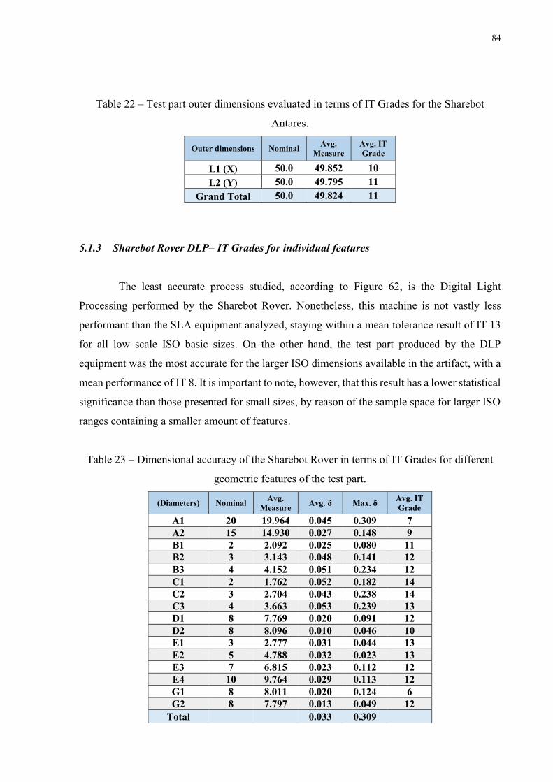
84

Table 22 – Test part outer dimensions evaluated in terms of IT Grades for the Sharebot

Antares.


Avg. IT Grade

L1 (X) 50.0 49.852 10 L2 (Y) 50.0 49.795 11

Grand Total 50.0 49.824 11

5.1.3 Sharebot Rover DLP– IT Grades for individual features

The least accurate process studied, according to Figure 62, is the Digital Light

Processing performed by the Sharebot Rover. Nonetheless, this machine is not vastly less

performant than the SLA equipment analyzed, staying within a mean tolerance result of IT 13

for all low scale ISO basic sizes. On the other hand, the test part produced by the DLP

equipment was the most accurate for the larger ISO dimensions available in the artifact, with a

mean performance of IT 8. It is important to note, however, that this result has a lower statistical

significance than those presented for small sizes, by reason of the sample space for larger ISO

ranges containing a smaller amount of features.

Table 23 – Dimensional accuracy of the Sharebot Rover in terms of IT Grades for different




Total 0.033 0.309

85

In the same analytical arrangement performed formerly performed, the results of the

Sharebot Rover for circular features is presented in

Table 23 above. Other than Concentric (A) and Horizontal Cylinders (G), all circular

features have been produced in the Sharebot Rover with tolerances above IT 11, yet averaging

IT 13. In terms of measurement precision and surface roughness, the SLA and DLP machines

have similar deviations (𝛿) in circular features, of 28 and 33 microns, respectively. This result,

when compared to a 9 micron deviation in PolyJet, shows a lesser performance in accuracy of

the Sharebot Rover and Antares machines when creating cylindrical components in AM.

Modifying the analysis to linear measurements, the lengths and heights of the Sharebot

Antares present much better results in some features. As seen in Table 24, features such as

Cylinder Boss (B) and Staircases (H1-9) have shown results better than those for SLA, where

B-features performed at an IT Grade of 11, and Staircases demonstrated prominence by

achieving grades as low as IT 5 and 6. The Staircase feature, however, did have a diverse

performance as a function of step heights, since accuracy varies from IT 5 (H4) up to IT 10

(H6). The mean performance of excavated (or negative) features in Staircases is more accurate

than protruding (or positive) features.


evaluated in terms of IT Grades for the Sharebot Rover.

Principal Dimensions Nominal Avg.


Cylinder Boss (height) B features 3.0 3.070 11 Pins (height) C features 3.0 2.245 > 16 Staircases (height)

H1 -4.0 3.977 6 H2 -3.0 3.008 6 H3 -2.0 1.972 9 H4 -1.0 1.001 5 H5 1.0 0.971 9 H6 2.0 1.953 10 H7 3.0 2.978 9 H8 4.0 3.984 7 H9 5.0 4.966 9

From Table 24 it is also noticeable that C-features, or Pins, have resulted in large

imprecisions when measured, with a mean error of 25% with respect to nominal values of the

artifact. The result of imprecision above IT 16 for Pins has been discarded from analysis, and

highlights a qualitative complication of DLP manufacturing systems. Digital Light Processing

86

systems and resin reservoir AM methods in general are subject to problems and imprecision

caused by unwanted resin curing. The Pins of the artifact consist of small 3 mm long openings,

in which the largest diameter is that of feature C3, with 4 mm. Therefore, the feature is subject

to unintended resin curing, that could be cause by inadequate washing of the part within post-

processing, incorrect setup of the ultrasonic cleaning equipment, or even nonattendance of the

part, being the last a likely hypothesis for the Sharebot Rover’s fabricated part. The part

produced turned out to have cured resin within small pockets, which was likely a byproduct of

the long fabrication time of the unit – production of the DLP part required roughly 14 hours.

The same effect can be observed in Rectangular Boss feature (J), displayed in Figure

64, since there are also entries and gaps that can amass liquid resin remains. Therefore, data in

Table 25 presents calculated tolerance grades particularly for outward rectangular features.

Builds in the XY plane, however, remain unaffected, and can still be computed for data analysis.

Finally, it is possible to observe that embossed rectangles produced by the Sharebot Rover are

expected to present a minimum tolerance grade of IT 10, scaling up to IT 12 in its least accurate

axis (X). Positive rectangular extrusions (J1-3; Z-axis), however, have been precisely produced

features both in SLA and PolyJet, with a modal grade of IT 8, whereas the modal grade observed

in DLP is considerably larger, at IT 10.

Figure 64 – Zoomed-in image of the DLP test-part’s Rectangular Boss (J) and Pins (C)

features where unintended curing had occurred.

87


of IT Grades for the Sharebot Rover.



X 3.0 2.945 12 Y 4.0 3.847 10 Z

J1 3.0 2.984 8 J2 5.0 4.935 10 J3 7.0 6.926 10 J4 -7.0 2.809 - J5 -5.0 3.651 - J6 -3.0 2.844 - J7 -1.0 0.824 -

Finally, Table 26 presents the analysis for Square Boss (F) geometries in the DLP test-

part. In this feature, it is noticeable how accuracy is affected as a function of manufacturing

direction. The Z-axis demonstrates the best accuracy grade, in IT 8, whilst in the XY plane

accuracy ranges from IT 14 to 15. Outer dimensions (L) for the Sharebot Rover achieved IT

grades of 12 in the x-axis and 14 in the y-axis, which is quite inaccurate for a large basic ISO

size.


Sharebot Rover.


Avg. IT Grade

F1 X 3.0 2.415 16 Y 3.0 2.487 15 Z 3.0 2.973 8 F2 X 6.0 5.492 15 Y 6.0 5.550 14 Z 3.0 2.922 8 F3 X 9.0 8.359 15 Y 9.0 8.501 14 Z 3.0 2.976 8

Table 27 – Test part outer dimensions evaluated in terms of IT Grades for the Sharebot Rover.


Avg. IT Grade

L1 (X) 50.0 49.696 12 L2 (Y) 50.0 49.228 14

Grand Total 50.0 49.462 13

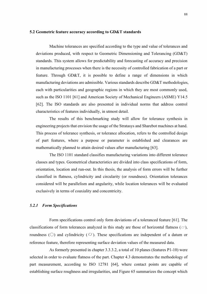
88

5.2 Geometric feature accuracy according to GD&T standards

Machine tolerances are specified according to the type and value of tolerances and

deviations produced, with respect to Geometric Dimensioning and Tolerancing (GD&T)

standards. This system allows for predictability and forecasting of accuracy and precision

in manufacturing processes when there is the necessity of controlled fabrication of a part or

feature. Through GD&T, it is possible to define a range of dimensions in which

manufacturing deviations are admissible. Various standards describe GD&T methodologies,

each with particularities and geographic regions in which they are most commonly used,

such as the ISO 1101 [61] and American Society of Mechanical Engineers (ASME) Y14.5

[62]. The ISO standards are also presented in individual norms that address control

characteristics of features individually, in utmost detail.

The results of this benchmarking study will allow for tolerance synthesis in

engineering projects that envision the usage of the Stratasys and Sharebot machines at hand.

This process of tolerance synthesis, or tolerance allocation, refers to the controlled design

of part features, where a purpose or parameter is established and clearances are

mathematically planned to attain desired values after manufacturing [63].

The ISO 1101 standard classifies manufacturing variations into different tolerance

classes and types. Geometrical characteristics are divided into class specifications of form,

orientation, location and run-out. In this thesis, the analysis of form errors will be further

classified in flatness, cylindricity and circularity (or roundness). Orientation tolerances

considered will be parallelism and angularity, while location tolerances will be evaluated

exclusively in terms of coaxiality and concentricity.

5.2.1 Form Specifications

Form specifications control only form deviations of a toleranced feature [61]. The

classifications of form tolerances analyzed in this study are those of horizontal flatness ( ),

roundness (○) and cylindricity ( ). These specifications are independent of a datum or

reference feature, therefore representing surface deviation values of the measured data.

As formerly presented in chapter 3.3.3.2, a total of 10 planes (features P1-10) were

selected in order to evaluate flatness of the part. Chapter 4.3 demonstrates the methodology of

part measurement, according to ISO 12781 [64], where contact points are capable of

establishing surface roughness and irregularities, and Figure 65 summarizes the concept which

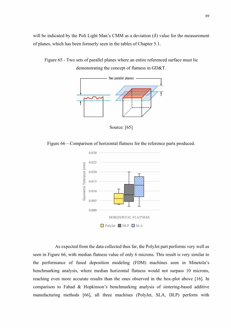
89

will be indicated by the Poli Light Man’s CMM as a deviation (𝛿) value for the measurement

of planes, which has been formerly seen in the tables of Chapter 5.1.

Figure 65 - Two sets of parallel planes where an entire referenced surface must lie

demonstrating the concept of flatness in GD&T.

Source: [65]

Figure 66 – Comparison of horizontal flatness for the reference parts produced.

As expected from the data collected thus far, the PolyJet part performs very well as

seen in Figure 66, with median flatness value of only 6 microns. This result is very similar to

the performance of fused deposition modeling (FDM) machines seen in Minetola’s

benchmarking analysis, where median horizontal flatness would not surpass 10 microns,

reaching even more accurate results than the ones observed in the box-plot above [16]. In

comparison to Fahad & Hopkinson’s benchmarking analysis of sintering-based additive

manufacturing methods [66], all three machines (PolyJet, SLA, DLP) perform with

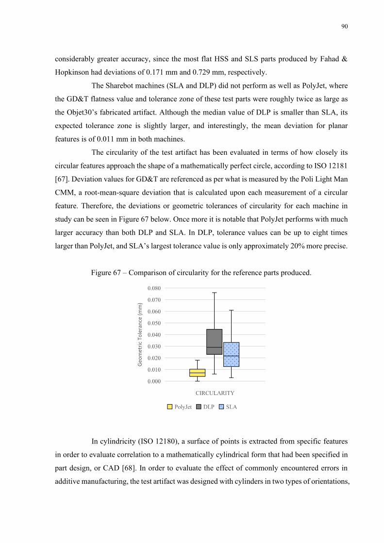
90

considerably greater accuracy, since the most flat HSS and SLS parts produced by Fahad &

Hopkinson had deviations of 0.171 mm and 0.729 mm, respectively.

The Sharebot machines (SLA and DLP) did not perform as well as PolyJet, where

the GD&T flatness value and tolerance zone of these test parts were roughly twice as large as

the Objet30’s fabricated artifact. Although the median value of DLP is smaller than SLA, its

expected tolerance zone is slightly larger, and interestingly, the mean deviation for planar

features is of 0.011 mm in both machines.

The circularity of the test artifact has been evaluated in terms of how closely its

circular features approach the shape of a mathematically perfect circle, according to ISO 12181

[67]. Deviation values for GD&T are referenced as per what is measured by the Poli Light Man

CMM, a root-mean-square deviation that is calculated upon each measurement of a circular

feature. Therefore, the deviations or geometric tolerances of circularity for each machine in

study can be seen in Figure 67 below. Once more it is notable that PolyJet performs with much

larger accuracy than both DLP and SLA. In DLP, tolerance values can be up to eight times

larger than PolyJet, and SLA’s largest tolerance value is only approximately 20% more precise.

Figure 67 – Comparison of circularity for the reference parts produced.

In cylindricity (ISO 12180), a surface of points is extracted from specific features

in order to evaluate correlation to a mathematically cylindrical form that had been specified in

part design, or CAD [68]. In order to evaluate the effect of commonly encountered errors in

additive manufacturing, the test artifact was designed with cylinders in two types of orientations,

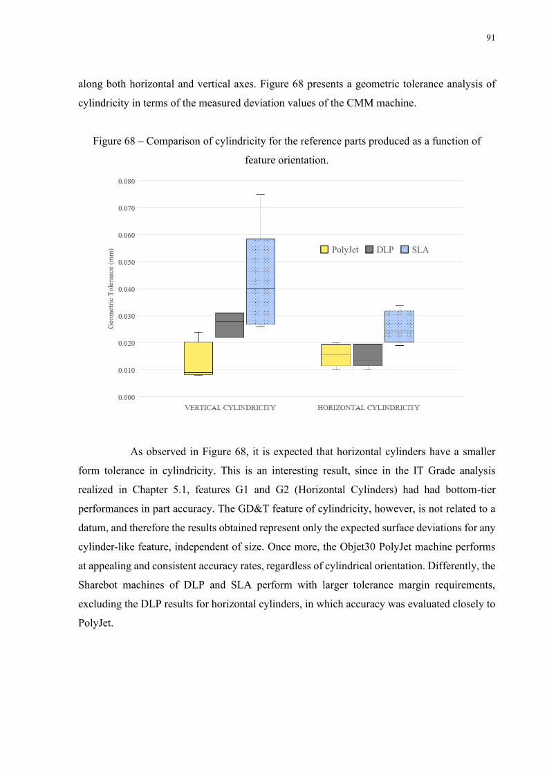
91

along both horizontal and vertical axes. Figure 68 presents a geometric tolerance analysis of

cylindricity in terms of the measured deviation values of the CMM machine.

Figure 68 – Comparison of cylindricity for the reference parts produced as a function of

feature orientation.

As observed in Figure 68, it is expected that horizontal cylinders have a smaller

form tolerance in cylindricity. This is an interesting result, since in the IT Grade analysis

realized in Chapter 5.1, features G1 and G2 (Horizontal Cylinders) had had bottom-tier

performances in part accuracy. The GD&T feature of cylindricity, however, is not related to a

datum, and therefore the results obtained represent only the expected surface deviations for any

cylinder-like feature, independent of size. Once more, the Objet30 PolyJet machine performs

at appealing and consistent accuracy rates, regardless of cylindrical orientation. Differently, the

Sharebot machines of DLP and SLA perform with larger tolerance margin requirements,

excluding the DLP results for horizontal cylinders, in which accuracy was evaluated closely to

PolyJet.

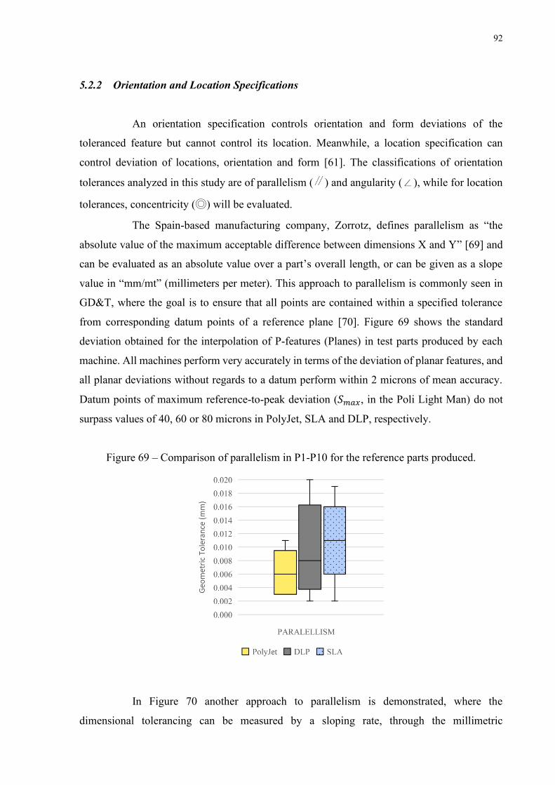
92

5.2.2 Orientation and Location Specifications

An orientation specification controls orientation and form deviations of the

toleranced feature but cannot control its location. Meanwhile, a location specification can

control deviation of locations, orientation and form [61]. The classifications of orientation

tolerances analyzed in this study are of parallelism ( ) and angularity (∠), while for location

tolerances, concentricity (◎) will be evaluated.

The Spain-based manufacturing company, Zorrotz, defines parallelism as “the

absolute value of the maximum acceptable difference between dimensions X and Y” [69] and

can be evaluated as an absolute value over a part’s overall length, or can be given as a slope

value in “mm/mt” (millimeters per meter). This approach to parallelism is commonly seen in

GD&T, where the goal is to ensure that all points are contained within a specified tolerance

from corresponding datum points of a reference plane [70]. Figure 69 shows the standard

deviation obtained for the interpolation of P-features (Planes) in test parts produced by each

machine. All machines perform very accurately in terms of the deviation of planar features, and

all planar deviations without regards to a datum perform within 2 microns of mean accuracy.

Datum points of maximum reference-to-peak deviation (𝑆𝑚𝑎𝑥, in the Poli Light Man) do not

surpass values of 40, 60 or 80 microns in PolyJet, SLA and DLP, respectively.

Figure 69 – Comparison of parallelism in P1-P10 for the reference parts produced.

In Figure 70 another approach to parallelism is demonstrated, where the

dimensional tolerancing can be measured by a sloping rate, through the millimetric

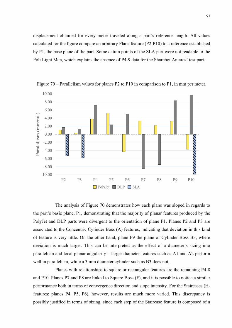
93

displacement obtained for every meter traveled along a part’s reference length. All values

calculated for the figure compare an arbitrary Plane feature (P2-P10) to a reference established

by P1, the base plane of the part. Some datum points of the SLA part were not readable to the

Poli Light Man, which explains the absence of P4-9 data for the Sharebot Antares’ test part.

Figure 70 – Parallelism values for planes P2 to P10 in comparison to P1, in mm per meter.

The analysis of Figure 70 demonstrates how each plane was sloped in regards to

the part’s basic plane, P1, demonstrating that the majority of planar features produced by the

PolyJet and DLP parts were divergent to the orientation of plane P1. Planes P2 and P3 are

associated to the Concentric Cylinder Boss (A) features, indicating that deviation in this kind

of feature is very little. On the other hand, plane P9 the plane of Cylinder Boss B3, where

deviation is much larger. This can be interpreted as the effect of a diameter’s sizing into

parallelism and local planar angularity – larger diameter features such as A1 and A2 perform

well in parallelism, while a 3 mm diameter cylinder such as B3 does not.

Planes with relationships to square or rectangular features are the remaining P4-8

and P10. Planes P7 and P8 are linked to Square Boss (F), and it is possible to notice a similar

performance both in terms of convergence direction and slope intensity. For the Staircases (H-

features; planes P4, P5, P6), however, results are much more varied. This discrepancy is

possibly justified in terms of sizing, since each step of the Staircase feature is composed of a

94

3x3 mm extrusion, which would lead to a similar conclusion of what has been seen in the

contrast of planes P2-3 and P9. The final plane, P10, is associated to negative Rectangular Boss

features (J4-J7). The results of parallelism in this plane are much less consistent, and greatly

more sloped since the surface area of the block that holds features J4-J7 is composed of fine

1 mm walls, which likely contribute to an imperceptible curvature of planes that are included

in the geometry. Accordingly, it is expected that the results of parallelism in plane P10 are

composed of large tolerance margins and likewise a lower statistical relevancy.

Finally, the last point of interest in terms of location and orientation specifications

lies within the latter and refers to the angularity of planes. In this study the benchmark of Incline

features (I) is based on instructions and standards defined in ISO 1101. In GD&T, “Angularity”

is defined as a parameter that does not control the angle of a referenced surface directly, but it

controls the envelope or tolerance zone in which the entire surface must lie [71]. From authorial

interest, the forthcoming analysis will contain a percentual error margin with regards to angular

deviation. The measurement procedure realized in Chapter 4.3 consists of an angular

comparison of the I-features’ slope to the base (reference plane), and therefore data points will

be sorted according to Equation (8), that can be visually understood from Figure 71.

(𝐴𝑛𝑔𝑢𝑙𝑎𝑟𝑖𝑡𝑦 𝑇𝑜𝑙𝑒𝑟𝑎𝑛𝑐𝑒) = 2𝑅𝐼 ∗ sin (𝛼𝑅 − 𝛼) (8)

Where:

• 𝑅𝐼 = 7.5 𝑚𝑚 is the general radius of all I-Features;

• 𝛼 is nominal angle of the incline;

• 𝛼𝑅 is real or measured angle of the incline.

Figure 71 – Outline of the adapted angularity tolerance zone calculated in this study.

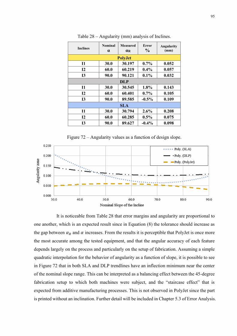
95

Table 28 – Angularity (mm) analysis of Inclines.

Inclines Nominal

α Measured

αR Error %

Angularity (mm)

PolyJet I1 30.0 30.197 0.7% 0.052 I2 60.0 60.219 0.4% 0.057 I3 90.0 90.121 0.1% 0.032

DLP I1 30.0 30.545 1.8% 0.143 I2 60.0 60.401 0.7% 0.105 I3 90.0 89.585 -0.5% 0.109

SLA I1 30.0 30.794 2.6% 0.208 I2 60.0 60.285 0.5% 0.075 I3 90.0 89.627 -0.4% 0.098

Figure 72 – Angularity values as a function of design slope.

It is noticeable from Table 28 that error margins and angularity are proportional to

one another, which is an expected result since in Equation (8) the tolerance should increase as

the gap between 𝛼𝑅 and 𝛼 increases. From the results it is perceptible that PolyJet is once more

the most accurate among the tested equipment, and that the angular accuracy of each feature

depends largely on the process and particularly on the setup of fabrication. Assuming a simple

quadratic interpolation for the behavior of angularity as a function of slope, it is possible to see

in Figure 72 that in both SLA and DLP trendlines have an inflection minimum near the center

of the nominal slope range. This can be interpreted as a balancing effect between the 45-degree

fabrication setup to which both machines were subject, and the “staircase effect” that is

expected from additive manufacturing processes. This is not observed in PolyJet since the part

is printed without an inclination. Further detail will be included in Chapter 5.3 of Error Analysis.

96

5.2.3 Cones and spheres

There are no definitions for cones or spheres in ISO 1101 standards for GD&T, and

therefore the deviation values evaluated for cones (K-features) and hemispheres (D-features)

must be observed under instruction of different norms. For cones, the ISO 3040 norm, and

spheres will be referenced through definitions contained in ISO 1132 of gauging and

tolerancing principles, and ISO 3290 of steel spheres for roller bearings.

According to the ISO 3040, tolerancing of a cone is intrinsically defined by its angle,

which can be defined through the cone’s angle (𝛼) or the rate of tapering (𝐶). Additionally, for

a fixed cone or finite geometry, a length (𝐿𝐴) or height can be used; The concept presented is

presented by the hypothetical cone of Figure 73.

Figure 73 – Intrinsic representation of a cone.

Source: [37]

Table 29 – Dimensional accuracy for cones in terms of angles and measure taper rates (mm).

CONE ANGLE Value of Angle Taper Rates

Nominal Avg. Measure Error CNOM. CMEAS.

PolyJet K1 30.0 29.4 -1.88% 0.536 0.525 K2 15.0 14.5 -3.39% 0.263 0.254

DLP K1 30.0 30.9 2.97% 0.536 0.553 K2 15.0 15.5 3.54% 0.263 0.273

SLA K1 30.0 29.7 -0.93% 0.536 0.531 K2 15.0 18.2 21.27% 0.263 0.320

Table 29 presents an error comparison between the angles that have been produced

and their CAD nominal values. The ration of 𝐶𝑀𝐸𝐴𝑆: 𝐶𝑁𝑂𝑀 portrays roughly the same error

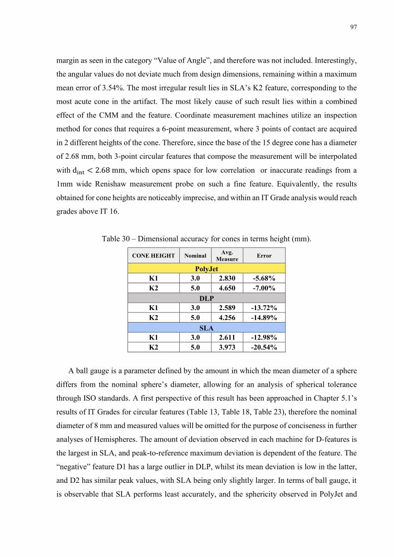
97

margin as seen in the category “Value of Angle”, and therefore was not included. Interestingly,

the angular values do not deviate much from design dimensions, remaining within a maximum

mean error of 3.54%. The most irregular result lies in SLA’s K2 feature, corresponding to the

most acute cone in the artifact. The most likely cause of such result lies within a combined

effect of the CMM and the feature. Coordinate measurement machines utilize an inspection

method for cones that requires a 6-point measurement, where 3 points of contact are acquired

in 2 different heights of the cone. Therefore, since the base of the 15 degree cone has a diameter

of 2.68 mm, both 3-point circular features that compose the measurement will be interpolated

with dint < 2.68 mm, which opens space for low correlation or inaccurate readings from a

1mm wide Renishaw measurement probe on such a fine feature. Equivalently, the results

obtained for cone heights are noticeably imprecise, and within an IT Grade analysis would reach

grades above IT 16.

Table 30 – Dimensional accuracy for cones in terms height (mm).

CONE HEIGHT Nominal Avg. Measure Error

PolyJet K1 3.0 2.830 -5.68% K2 5.0 4.650 -7.00%

DLP K1 3.0 2.589 -13.72% K2 5.0 4.256 -14.89%

SLA K1 3.0 2.611 -12.98% K2 5.0 3.973 -20.54%

A ball gauge is a parameter defined by the amount in which the mean diameter of a sphere

differs from the nominal sphere’s diameter, allowing for an analysis of spherical tolerance

through ISO standards. A first perspective of this result has been approached in Chapter 5.1’s

results of IT Grades for circular features (Table 13, Table 18, Table 23), therefore the nominal

diameter of 8 mm and measured values will be omitted for the purpose of conciseness in further

analyses of Hemispheres. The amount of deviation observed in each machine for D-features is

the largest in SLA, and peak-to-reference maximum deviation is dependent of the feature. The

“negative” feature D1 has a large outlier in DLP, whilst its mean deviation is low in the latter,

and D2 has similar peak values, with SLA being only slightly larger. In terms of ball gauge, it

is observable that SLA performs least accurately, and the sphericity observed in PolyJet and

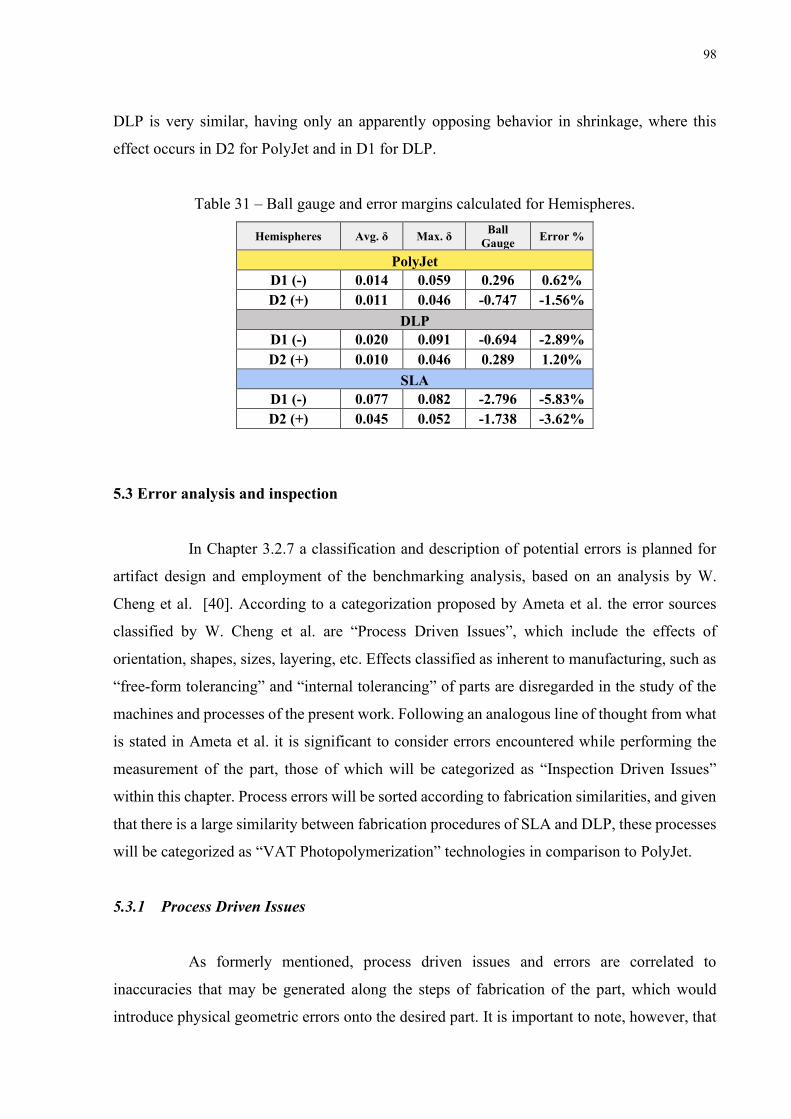
98

DLP is very similar, having only an apparently opposing behavior in shrinkage, where this

effect occurs in D2 for PolyJet and in D1 for DLP.

Table 31 – Ball gauge and error margins calculated for Hemispheres.

Hemispheres Avg. δ Max. δ Ball Gauge Error %

PolyJet D1 (-) 0.014 0.059 0.296 0.62% D2 (+) 0.011 0.046 -0.747 -1.56%

DLP D1 (-) 0.020 0.091 -0.694 -2.89% D2 (+) 0.010 0.046 0.289 1.20%

SLA D1 (-) 0.077 0.082 -2.796 -5.83% D2 (+) 0.045 0.052 -1.738 -3.62%

5.3 Error analysis and inspection

In Chapter 3.2.7 a classification and description of potential errors is planned for

artifact design and employment of the benchmarking analysis, based on an analysis by W.

Cheng et al. [40]. According to a categorization proposed by Ameta et al. the error sources

classified by W. Cheng et al. are “Process Driven Issues”, which include the effects of

orientation, shapes, sizes, layering, etc. Effects classified as inherent to manufacturing, such as

“free-form tolerancing” and “internal tolerancing” of parts are disregarded in the study of the

machines and processes of the present work. Following an analogous line of thought from what

is stated in Ameta et al. it is significant to consider errors encountered while performing the

measurement of the part, those of which will be categorized as “Inspection Driven Issues”

within this chapter. Process errors will be sorted according to fabrication similarities, and given

that there is a large similarity between fabrication procedures of SLA and DLP, these processes

will be categorized as “VAT Photopolymerization” technologies in comparison to PolyJet.

5.3.1 Process Driven Issues

As formerly mentioned, process driven issues and errors are correlated to

inaccuracies that may be generated along the steps of fabrication of the part, which would

introduce physical geometric errors onto the desired part. It is important to note, however, that

99

error sources will be observed individually within this chapter, and in actuality the results

observed are a combination of multiple effects onto the geometric features.

In terms of importing a CAD file, approximations are made so that the designed

part is understandable to the manufacturing machines, thus the model is converted to a Standard

Tessellation Language file (STL) [72]. This conversion from CAD to STL introduces an error

commonly known as “chordal error”, which is the maximum deviation between an original

CAD surface and a triangulation of a tessellated model [73]. This error is a potential cause of

inaccuracies within the parts fabricated in RMLAB’s Sharebot and Stratasys machines,

however it is expected that the influence of this effect would be of only a small margin of

micrometers. Nevertheless, Tessellation errors can be avoided through the usage of different

file formats from the common STL type. Recently, other file formats such as Jupiter

Tessellation (JT) and Additive Manufacturing File (AMF) have been proposed [74][75]. Such

formats, however, have not been extensively accepted by machine manufacturers due to the

larger complexity involved in CAD surface slicing, in addition to how widespread and simple

STL has become over time.

The effect entitled as “missing feature” by W. Cheng et al. is exhibited in Figure 74

and shows how geometries and features may be distorted in uniform slicing procedures [76].

The results of this effect are likely seen in features whose precision is evaluated in terms of

heights on the Z-axis. Since the VAT parts produced in Sharebot machines are tilted at an angle

of 45 degrees, it is expected that this effect would materialize larger inaccuracies than in PolyJet.

The effect can be seen clearly when contrasting the results presented by Table 14 to its

counterparts in VAT Sharebot machines. Not only is the layer thickness of PolyJet as fine as

the VAP parts, but orientation allows for topology-optimized prints, in which the influence of

the “missing feature” and staircase effects is not as expected. Furthermore, as seen in Table 30,

the error in heights of Cones (K) in VAT features is much larger than PolyJet, where error

percentages are roughly 2 or 3 times greater. It is also noticeable how the larger feature (K2)

presents a higher error margin, which is likely to be a contribution of the “missing feature”

effect, where a slimmer feature’s tip is more likely to be approximated to an absent piece in the

layer.

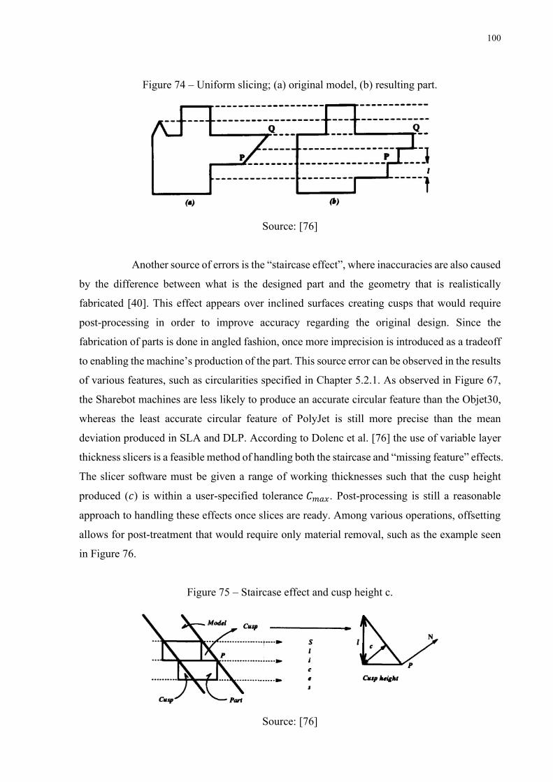
100

Figure 74 – Uniform slicing; (a) original model, (b) resulting part.

Source: [76]

Another source of errors is the “staircase effect”, where inaccuracies are also caused

by the difference between what is the designed part and the geometry that is realistically

fabricated [40]. This effect appears over inclined surfaces creating cusps that would require

post-processing in order to improve accuracy regarding the original design. Since the

fabrication of parts is done in angled fashion, once more imprecision is introduced as a tradeoff

to enabling the machine’s production of the part. This source error can be observed in the results

of various features, such as circularities specified in Chapter 5.2.1. As observed in Figure 67,

the Sharebot machines are less likely to produce an accurate circular feature than the Objet30,

whereas the least accurate circular feature of PolyJet is still more precise than the mean

deviation produced in SLA and DLP. According to Dolenc et al. [76] the use of variable layer

thickness slicers is a feasible method of handling both the staircase and “missing feature” effects.

The slicer software must be given a range of working thicknesses such that the cusp height

produced (𝑐) is within a user-specified tolerance 𝐶𝑚𝑎𝑥. Post-processing is still a reasonable

approach to handling these effects once slices are ready. Among various operations, offsetting

allows for post-treatment that would require only material removal, such as the example seen

in Figure 76.

Figure 75 – Staircase effect and cusp height c.

Source: [76]

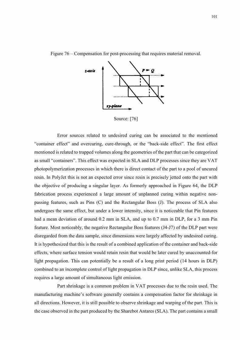
101

Figure 76 – Compensation for post-processing that requires material removal.

Source: [76]

Error sources related to undesired curing can be associated to the mentioned

“container effect” and overcuring, cure-through, or the “back-side effect”. The first effect

mentioned is related to trapped volumes along the geometries of the part that can be categorized

as small “containers”. This effect was expected in SLA and DLP processes since they are VAT

photopolymerization processes in which there is direct contact of the part to a pool of uncured

resin. In PolyJet this is not an expected error since resin is precisely jetted onto the part with

the objective of producing a singular layer. As formerly approached in Figure 64, the DLP

fabrication process experienced a large amount of unplanned curing within negative non-

passing features, such as Pins (C) and the Rectangular Boss (J). The process of SLA also

undergoes the same effect, but under a lower intensity, since it is noticeable that Pin features

had a mean deviation of around 0.2 mm in SLA, and up to 0.7 mm in DLP, for a 3 mm Pin

feature. Most noticeably, the negative Rectangular Boss features (J4-J7) of the DLP part were

disregarded from the data sample, since dimensions were largely affected by undesired curing.

It is hypothesized that this is the result of a combined application of the container and back-side

effects, where surface tension would retain resin that would be later cured by unaccounted-for

light propagation. This can potentially be a result of a long print period (14 hours in DLP)

combined to an incomplete control of light propagation in DLP since, unlike SLA, this process

requires a large amount of simultaneous light emission.

Part shrinkage is a common problem in VAT processes due to the resin used. The

manufacturing machine’s software generally contains a compensation factor for shrinkage in

all directions. However, it is still possible to observe shrinkage and warping of the part. This is

the case observed in the part produced by the Sharebot Antares (SLA). The part contains a small

102

amount of warpage noticeable only on the bottom face of the part, as seen in Figure 78. Similar

to the process observed in Mahesh et. al [21] the part displayed warpage on one side (Figure

77-b).

Figure 77 – Part warpage drifting towards edges (a) and only one side (b).

Source: [21]

Figure 78 – SLA part (left) and PolyJet (right) highlighting the warped edge of the SLA part.

Shrinkage of resin during photo-polymerization is the major cause of errors during

the SLA process. There are two types of shrinkage that occur due to the photopolymer’s reaction.

The first is caused by the formation of the polymer bond. Since the pre-polymer liquid resin

state is less dense than the solidified (or already cured) polymer, the volume of the cured solid

is smaller than the volume of liquid from which it was formed. The second cause of shrinkage

is a thermal effect that results from the exothermic nature of photo-polymerization. Sudden

heating causes the photopolymer to expand upon formation, and at the same time heat is lost to

the surroundings, developing the shrinking effect. The combination of these types of shrinkage

is known to result in internal stresses that lead to part warping [60] [77].

103

It is also possible that deformations in the edges and inferior base of the SLA test

part were a result of insufficient supporting structures, since inverted stereolithography – as

performed by the Sharebot Antares – requires larger support structures to keep the part attached

to the build platform, and uncoupling could have been a cause to the distortion [78]. Also, in

SLA sagging and unwanted bending are likely to occur since in this manufacturing method

requires post-process UV curing for the parts to achieve full strength and become stable [79].

Conclusively, in order to ensure the absence of problematic warping and shrinkage,

or even simply reduce distortion if it is significant enough, the user must factor the orientation

of the part, its position on the build platform, power of light emission, temperature of the build

platform, supporting sufficiency and the feasibility of brims and rafts. It is worth mentioning

that the SLA part evaluated in this study had a minor one-sided warping effect that had

negligible influence on the accuracy of geometries contained on the upper face of the part.

5.3.2 Inspection Driven Issues

Considering the aforementioned sources of error, it is also important to understand

that inspection may also be a source of errors and uncertainties. As mentioned in Chapter 3.2.5,

the Poli Light Man has a maximum permissible error (MPE), and this parameter of a CMM

must be accounted for when considering possible sources of inaccuracies. The machine has a

declared volumetric length measuring uncertainty of MPE 5 + 10*L, where L is the measured

length.

A typical stylus used for CMM measurements is composed of a spherical tip at the

end of the stylus shaft, as formerly seen in Chapter 3.2.5, in order to maintain a uniform shape

in all relevant directions. Measurements and the dimensions of a workpiece are calculated based

on the probing coordinates, therefore calibration of what is called the “form error” of a probe

tip is essential in 3D measurements by a coordinate measurement machine. The order of form

error in styli, however, is very minor, with a range of tens of nanometers when tests are

performed on gauge blocks with ultra-flat surfaces [80]. Therefore, the effect of stylus error is

negligible in this study, since the artifact features contain geometries in the range of millimeters,

and precision is evaluated in a scale of micrometers.

104

6. CONCLUSION

The benchmarking study that was conducted in this thesis depicts the qualities of

each machine analyzed, highlighting the performance in geometric accuracy of the Stratasys

Objet30 Prime PolyJet printer, over the Sharebot Antares and Sharebot Rover. The IT grade

analysis quantifies the discrepancy in performance, indicating that the Stratasys machine is

capable of performing within grades of IT 8 to 9, whilst the Sharebot equipment manufactures

at a range of IT 11 to 13.

Such difference in performance can be attributed to multiple factors, such as having

a more advanced and costly machine in the Objet30, with various automated features provided

by Stratasys. Moreover, the part is produced without the inclusion of supporting structures, in

its designed orientation and with a fine layering quality, which are factors capable of ensuring

higher accuracy and detail to an AM part. The absence of a resin vat – in contrast to the Sharebot

machines – also contributes to a minimization of error sources originated from fluid tension and

layer adhesion, preventing some possible distortions and warpage of the workpiece.

Regarding GD&T, the results indicate that the Sharebot machines are capable of

performing closely in accuracy to that which can be manufactured in an Objet30, especially

regarding the Sharebot Rover. Contrarily to what was initially expected, the Sharebot Rover

outperforms the Antares in most geometries, and in some demonstrates a median accuracy range

remarkably similar to what is fabricated in PolyJet. It is interesting that when ISO basic sizes

of fabrication dimensions are compared, the Sharebot machines progress into better accuracies

as the size of the part increases. On the other hand, the Objet30 performed consistently within

its expected IT grade range, even when dimensions are in much larger basic sizes.

It is scientifically relevant to recognize improvement points of the study performed,

and these can be categorized within the part design or experimental assessments. In terms of

artifact design, perfecting of the test part includes the rearrangement and restructuring of

features such as the square notch feature M1 and the enclosed spaces found in families C, H

and J. The slim wall in the square feature mentioned had obstructed measurements, therefore it

turns against initial design intentions. In the case of enclosed spaces, manufacturing with resins

caused minor undesired curing, which disables features for measurement, and therefore

removes their statistical relevancy in the analysis. This can be solved through the inclusion of

punctures in the features, which would allow resin to escape the confinement whilst also not

influencing the major geometry of the feature. It is also possible to include more inclines and

planar features along main geometries, for a better utilization of space and material.

105

With regards to fabrication, measurements and overall experimental assessments,

there is room for improvement of the study in different aspects. An alternative approach to that

which was performed is to fabricate more than one test part per machine, either in a batch that

is produced in the same session, or made in different moments, individually. This allows for a

larger framework of data, in which the same geometry can be observed multiple times with

regards to session or build platform area used. Another experimental enhancement that could

increase statistical relevancy is fabrication of all parts in the same orientation. Since the PolyJet

artifact was produced in design orientation, it is possible that the results observed for the

Objet30 had been favored over the Sharebot machines, in which parts were inclined when

fabricated.

Finally, it is important to note that data may have been influenced by the equipment

used when conducting the measurement procedures. In particular, it is important to be wary of

the CMM used, where manual measurement and calibration was conducted. The Poli Light Man

used not only is manual but contains aging equipment that dates to 1992, and other newer, more

precise, and advanced CMMs were not available for use at Politecnico di Torino. It is likely

that more modern technology would be capable of minimizing human errors or measurement

imprecisions that are propagated into the data.

The methodology presented in this dissertation has general applicability and can

also be extended to other additive manufacturing systems that utilize photopolymers. As

mentioned, over these first results it is possible to work towards an improvement of results, but

the analysis performed is complete and allows for predictability when using the Stratasys and

Sharebot equipment analyzed, which is the objective of the benchmarking analysis.

106

REFERENCES

[1] I. Newton and R. Hooke, “Isaac Newton letter to Robert Hooke,” 1675.

[2] J. Horn, L. N. Rosenband, and M. R. Smith, Reconceptualizing the Industrial

Revolution. 2010.

[3] K. Pouspourika, “The 4 Industrial Revolutionso Title,” 2019. [Online]. Available:

https://ied.eu/project-updates/the-4-industrial-revolutions/.

[4] J. S. Hyatt and J. W. Hyatt, “Improvement in Process and Apparatus for Manufacturing

Pyroxyline,” US133229A, 1872.

[5] R. F. Jones, “Tools of the Trade,” Astounding Science Fiction, 1950.

[6] D. E. H. Jones, “Ariadne,” New Sci., vol. 64, no. 917, p. 80, 1974.

[7] General Electric Additive, “ADDITIVE MANUFACTURING,” 2020. [Online].

Available: https://www.ge.com/additive/additive-manufacturing.

[8] T. Gornet and T. Wohlers, “History of Additive Manufacturing,” Wohlers Rep. 2014,

pp. 1–24, 2014.

[9] MANUFACTUR3D, “A Comprehensive List of All 3D Printing Technologies,” 2018.

[Online]. Available: https://manufactur3dmag.com/comprehensive-list-all-3d-printing-

technologies/.

[10] S. Crump, “FDM Stratasys Patent US 5,121,329,” 1992.

[11] C. R. Deckard, “SLS Patent US 4,863,538,” Google Patents, 1986.

[12] L. J. Hornbeck, “SPATIAL LIGHT MODULATOR AND METHOD Patent US

4,662,746,” 1987.

[13] C. W. Hull, “Apparatus for Production of Three-Dmensonal Objects By Stereo

Thography,” Google Patents, no. 19, p. 16, 1984.

[14] B. Kelly, I. Bhattacharya, M. Shusteff, R. M. Panas, H. K. Taylor, and C. M.

Spadaccini, “Computed Axial Lithography (CAL): Toward Single Step 3D Printing of

Arbitrary Geometries,” 2017.

[15] N. Sridharan and C. M. Petrie, “Ultrasonic Additive Manufacturing,” Additive

Manufacturing Processes. pp. 247–260, 2020.

[16] P. Minetola, L. Iuliano, and G. Marchiandi, “Benchmarking of FDM Machines through

Part Quality Using IT Grades,” Procedia CIRP, vol. 41, pp. 1027–1032, 2016.

[17] M. A. D. S.Moylan, J. Slotwinski, A. Cooke, K. Jurrens, “Proposal For a Standardized

Test Artifact For Additive Manufacturing Machines and Processes,” Solid Free. Fabr.

107

Symp., pp. 902–920, 2012.

[18] E. P. Gargiulo, “Stereolithography process accuracy: user experience, Proceedings of

the 1st European Conference on Rapid Prototyping,” 1992.

[19] J. P. Kruth, “Material Incress Manufacturing by Rapid Prototyping Techniques,” CIRP

Ann. - Manuf. Technol., vol. 40, no. 2, pp. 603–614, 1991.

[20] R. Ippolito, L. Iuliano, and A. Gatto, “Benchmarking of Rapid Protoyping Techniques

in Terms of Dimensional Accuracy and Surface Finish,” 1995.

[21] M. Mahesh, Y. S. Wong, J. Y. H. Fuh, and H. T. Loh, “Benchmarking for comparative

evaluation of RP systems and processes,” Rapid Prototyp. J., vol. 10, no. 2, pp. 123–

135, 2004.

[22] N. Decker and A. Yee, “A simplified benchmarking model for the assessment of

dimensional accuracy in FDM processes,” Int. J. Rapid Manuf., vol. 5, p. 145, Dec.

2016.

[23] F. A. Cruz Sanchez, H. Boudaoud, L. Muller, and M. Camargo, “Towards a standard

experimental protocol for open source additive manufacturing: This paper proposes a

benchmarking model for evaluating accuracy performance of 3D printers,” Virtual

Phys. Prototyp., vol. 9, no. 3, pp. 151–167, 2014.

[24] D. Flack, CMM Measurement Stategies - Good practice guide No. 41, no. 2. 2014.

[25] M. Fahad and N. Hopkinson, “A new benchmarking part for evaluating the accuracy

and repeatability of AM processes,” 2012.

[26] N. P. Juster and T. H. C. Childs, “A comparison of rapid prototyping processes,” in

Proceedings of Third European Conference on Rapid Prototyping and Manufacturing,

1994, pp. 35–52.

[27] Sharebot, “Sharebot Antares Technical Details Flyer,” Technical Datasheet, 2018.

[28] Sharebot, “Sharebot Antares: Professional SLA 3D printer with 15.000 cm3 of printing

volume.” [Online]. Available: https://www.sharebot.it/en/sharebot-antares-3d-printer/.

[29] Sharebot, “Sharebot Rover DLP Printer Technical Details Commercial Sheet,” 2019.

[30] Stratasys, “Objet30 Prime Technical Datasheet,” 2016.

[31] Stratasys, “Specification Sheet Objet350 - Connex3,” 2018.

[32] K. America, “Measurement System Types and Characteristics | Measurement

Fundamentals.” [Online]. Available: https://www.keyence.com/ss/products/measure-

sys/measurement-selection/type/.

[33] Donato Pimazzoni, “Macchine usato – Pimazzoni Cmm Service.” [Online]. Available:

https://www.pimazzonicmmservice.it/macchine-usato/.

108

[34] ISO 10360-2:2009, “Geometrical product specifications (GPS) — Acceptance and

reverification tests for coordinate measuring machines (CMM) — Part 2: CMMs used

for measuring linear dimensions,” 2009.

[35] Hexagon Manufacturing Intelligence, “All about CMM Styli,” 2014. [Online].

Available: https://www.hexagonmi.com/solutions/technical-resources/metrology-

101/what-is-a-cmm-stylus#:~:text=All about CMM Styli,the component to be

measured.

[36] E. W. Weisstein, “Cylinder,” MathWorld -- A Wolfram Web Resource. [Online].

Available: https://mathworld.wolfram.com/Cylinder.html.

[37] International Organization for Standardization, “Geometrical product specifications

(GPS) — Dimensioning and tolerancing — Cones,” vol. 20, 2016.

[38] Bearing News, “Additive manufacturing of rolling bearings in innovative lightweight

design by laser metal deposition,” 2019. [Online]. Available: https://www.bearing-

news.com/additive-manufacturing-of-rolling-bearings-in-innovative-lightweight-

design-by-laser-metal-deposition/.

[39] Oxford Learner’s Dictionary, “Sphere.” [Online]. Available:

https://www.oxfordlearnersdictionaries.com/us/definition/american_english/sphere.

[40] H. T. Loh, “Optimization of Part- Building Orientation in Stereolithography,” vol. 1,

no. 4, pp. 12–23, 2002.

[41] P. Kulkarni, A. Marsan, and D. Dutta, “Review of process planning techniques in

layered manufacturing,” Rapid Prototyp. J., vol. 6, no. 1, pp. 18–35, 2000.

[42] Z. D. Pritchard, M. P. de Beer, R. J. Whelan, T. F. Scott, and M. A. Burns, “Modeling

and Correcting Cure-Through in Continuous Stereolithographic 3D Printing,” Adv.

Mater. Technol., vol. 4, no. 12, pp. 1–7, 2019.

[43] P. . Jacobs, Rapid Prototyping and Manufacturing: Fundamentals of Stereo-

Lithography. Southfield, MI, USA: Society of Manufacturing Engineers, 1992.

[44] E. Yasa, O. Poyraz, E. U. Solakoglu, G. Akbulut, and S. Oren, “A Study on the Stair

Stepping Effect in Direct Metal Laser Sintering of a Nickel-based Superalloy,”

Procedia CIRP, vol. 45, pp. 175–178, 2016.

[45] H. Brooks, A. Rennie, T. Abram, J. McGovern, and F. Caron, “Variable Fused

Deposition Modelling - analysis of benefits, concept design and tool path generation,”

2011, pp. 511–517.

[46] D. Chakravorty, “3D Printing Support Structures,” 2020. [Online]. Available:

https://all3dp.com/1/3d-printing-support-structures/.

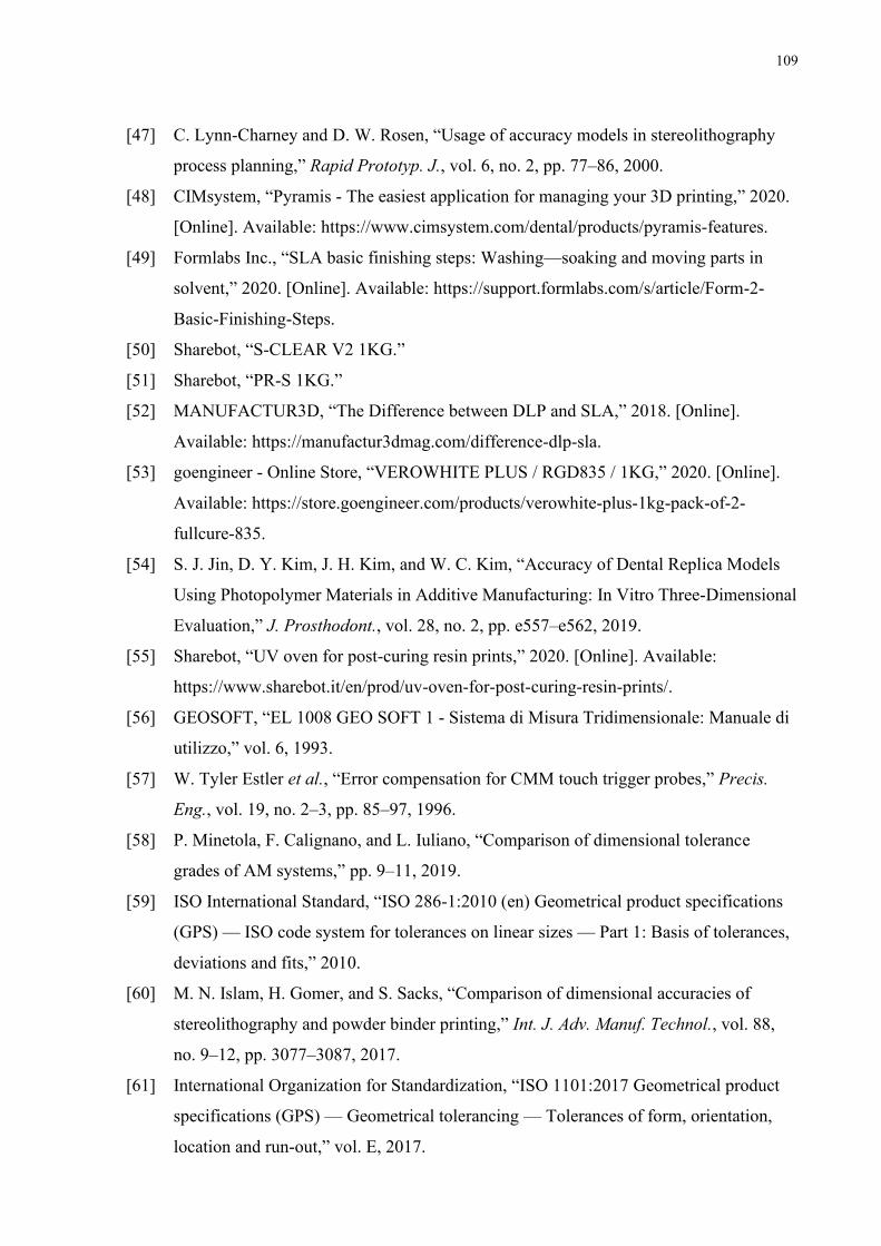
109

[47] C. Lynn-Charney and D. W. Rosen, “Usage of accuracy models in stereolithography

process planning,” Rapid Prototyp. J., vol. 6, no. 2, pp. 77–86, 2000.

[48] CIMsystem, “Pyramis - The easiest application for managing your 3D printing,” 2020.

[Online]. Available: https://www.cimsystem.com/dental/products/pyramis-features.

[49] Formlabs Inc., “SLA basic finishing steps: Washing—soaking and moving parts in

solvent,” 2020. [Online]. Available: https://support.formlabs.com/s/article/Form-2-

Basic-Finishing-Steps.

[50] Sharebot, “S-CLEAR V2 1KG.”

[51] Sharebot, “PR-S 1KG.”

[52] MANUFACTUR3D, “The Difference between DLP and SLA,” 2018. [Online].

Available: https://manufactur3dmag.com/difference-dlp-sla.

[53] goengineer - Online Store, “VEROWHITE PLUS / RGD835 / 1KG,” 2020. [Online].

Available: https://store.goengineer.com/products/verowhite-plus-1kg-pack-of-2-

fullcure-835.

[54] S. J. Jin, D. Y. Kim, J. H. Kim, and W. C. Kim, “Accuracy of Dental Replica Models

Using Photopolymer Materials in Additive Manufacturing: In Vitro Three-Dimensional

Evaluation,” J. Prosthodont., vol. 28, no. 2, pp. e557–e562, 2019.

[55] Sharebot, “UV oven for post-curing resin prints,” 2020. [Online]. Available:

https://www.sharebot.it/en/prod/uv-oven-for-post-curing-resin-prints/.

[56] GEOSOFT, “EL 1008 GEO SOFT 1 - Sistema di Misura Tridimensionale: Manuale di

utilizzo,” vol. 6, 1993.

[57] W. Tyler Estler et al., “Error compensation for CMM touch trigger probes,” Precis.

Eng., vol. 19, no. 2–3, pp. 85–97, 1996.

[58] P. Minetola, F. Calignano, and L. Iuliano, “Comparison of dimensional tolerance

grades of AM systems,” pp. 9–11, 2019.

[59] ISO International Standard, “ISO 286-1:2010 (en) Geometrical product specifications

(GPS) — ISO code system for tolerances on linear sizes — Part 1: Basis of tolerances,

deviations and fits,” 2010.

[60] M. N. Islam, H. Gomer, and S. Sacks, “Comparison of dimensional accuracies of

stereolithography and powder binder printing,” Int. J. Adv. Manuf. Technol., vol. 88,

no. 9–12, pp. 3077–3087, 2017.

[61] International Organization for Standardization, “ISO 1101:2017 Geometrical product

specifications (GPS) — Geometrical tolerancing — Tolerances of form, orientation,

location and run-out,” vol. E, 2017.

110

[62] ASME, “ASME Y14.5-2018 Dimensioning and Tolerancing.” New York, NY, 2018.

[63] B. C. Zhang, “Geometric modeling of dimensioning and tolerancing,” Arizona State

University, 1992.

[64] International Organization for Standardization, “ISO 12781-1:2011(en) Geometrical

product specifications (GPS) — Flatness — Part 1: Vocabulary and parameters of

flatness,” 2011.

[65] GD&T Basics, “FLATNESS,” 2014. [Online]. Available:

https://www.gdandtbasics.com/flatness/.

[66] M. Fahad and N. Hopkinson, “Evaluation and comparison of geometrical accuracy of

parts produced by sintering-based additive manufacturing processes,” Int. J. Adv.

Manuf. Technol., vol. 88, no. 9–12, pp. 3389–3394, 2017.


product specifications (GPS) — Roundness — Part 1: Vocabulary and parameters of

roundness.” 2011.


product specifications (GPS) — Cylindricity — Part 1: Vocabulary and parameters of

cylindrical form.” 2011.

[69] ZORROTZ, “Machine Tool Slide-ways.” p. 16, 2019.

[70] GD&T Basics, “PARALLELISM,” 2014. [Online]. Available:

https://www.gdandtbasics.com/parallelism/.

[71] GD&T Basics, “ANGULARITY.” [Online]. Available:

https://www.gdandtbasics.com/angularity/.

[72] N. Panhalkar, “Hierarchical Data Structures for Optimization of Additive

Manufacturing Processes,” 2015.

[73] J. Zhao, R. Xia, W. Liu, and H. Wang, “A computing method for accurate slice

contours based on an STL model,” Virtual Phys. Prototyp., vol. 4, no. 1, pp. 29–37,

2009.

[74] Siemens PLM Software, “JT File Format Reference Version 9.5 Rev-E.” 2010.

[75] ASTM, “Standard Specification for Additive Manufacturing File Format (AMF),”

2012.

[76] A. Dolenc and I. Mäkelä, “Slicing procedures for layered manufacturing techniques,”

Comput. Des., vol. 26, no. 2, pp. 119–126, 1994.

[77] W. Freed, Hull CW, L. CW, S. DR, S. ST, and V. WB, “Stereolithographic curl

reduction,” 1989.

111

[78] Formlabs Inc., “The Ultimate Guide to Stereolithography (SLA) 3D Printing,” no.

March, pp. 1–23, 2017.

[79] B. Redwood, “Dimensional accuracy of 3D printed parts,” 3D HUBS. [Online].

Available: https://www.3dhubs.com/knowledge-base/dimensional-accuracy-3d-printed-

parts/#sla.

[80] S. Ito, D. Tsutsumi, K. Kamiya, K. Matsumoto, and N. Kawasegi, “Measurement of

form error of a probe tip ball for coordinate measuring machine (CMM) using a

rotating reference sphere,” Precis. Eng., vol. 61, no. Cmm, pp. 41–47, 2020.

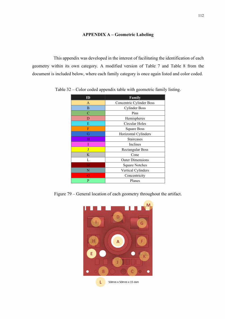
112

APPENDIX A – Geometric Labeling

This appendix was developed in the interest of facilitating the identification of each

geometry within its own category. A modified version of Table 7 and Table 8 from the

document is included below, where each family category is once again listed and color coded.

Table 32 – Color coded appendix table with geometric family listing.

ID Family A Concentric Cylinder Boss B Cylinder Boss C Pins D Hemispheres E Circular Holes F Square Boss G Horizontal Cylinders H Staircases I Inclines J Rectangular Boss K Cone L Outer Dimensions M Square Notches N Vertical Cylinders O Concentricity P Planes

Figure 79 – General location of each geometry throughout the artifact.

113

Figure 79 above associates the information presented in Table 32 to the physical

location of each geometry in the artifact part. The following figures will discriminate and label

each geometry within a specific category. Strictly speaking, each individual geometry will be

designated a letter and number with which it will become distinguishable.

Figure 80 – Geometric labelling for A, B, C and L.

Figure 81 – Geometric labelling for D, E, I, K, G.

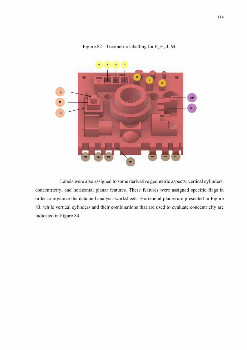
114

Figure 82 – Geometric labelling for F, H, J, M.

Labels were also assigned to some derivative geometric aspects: vertical cylinders,

concentricity, and horizontal planar features. These features were assigned specific flags in

order to organize the data and analysis worksheets. Horizontal planes are presented in Figure

83, while vertical cylinders and their combinations that are used to evaluate concentricity are

indicated in Figure 84.

115

Figure 83 – Geometric labelling for horizontal planes (P).

Figure 84 – Geometric labelling for concentricity (O).

Figure 85 – Combination of labels regarding concentricity.

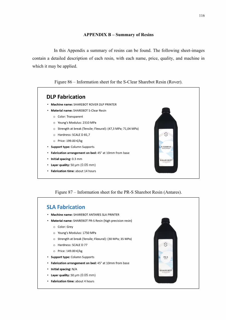
116

APPENDIX B – Summary of Resins

In this Appendix a summary of resins can be found. The following sheet-images

contain a detailed description of each resin, with each name, price, quality, and machine in

which it may be applied.

Figure 86 – Information sheet for the S-Clear Sharebot Resin (Rover).

Figure 87 – Information sheet for the PR-S Sharebot Resin (Antares).

117

Figure 88 – Information sheet for the VeroWhitePlus RGD835 Resin (Objet30).

118

APPENDIX C – Manufacturing Images

In this Appendix a group of images that refer to the fabrication of each replica have

been attached. All images are of self-authorship and have been prepared in the laboratorial

spaces of Politecnico di Torino.

I. SHAREBOT ROVER – DLP MANUFACTURING

Figure 89 – Sharebot Rover machine at Politecnico di Torino.

Figure 90 – Sharebot Rover details with respect to the build platform and resin vat.

119

Figure 91 – Sharebot Rover upon initialization of the manufacturing process.

Figure 92 - Sharebot Rover after completion of the part; Highlights produced artifact and

supports.

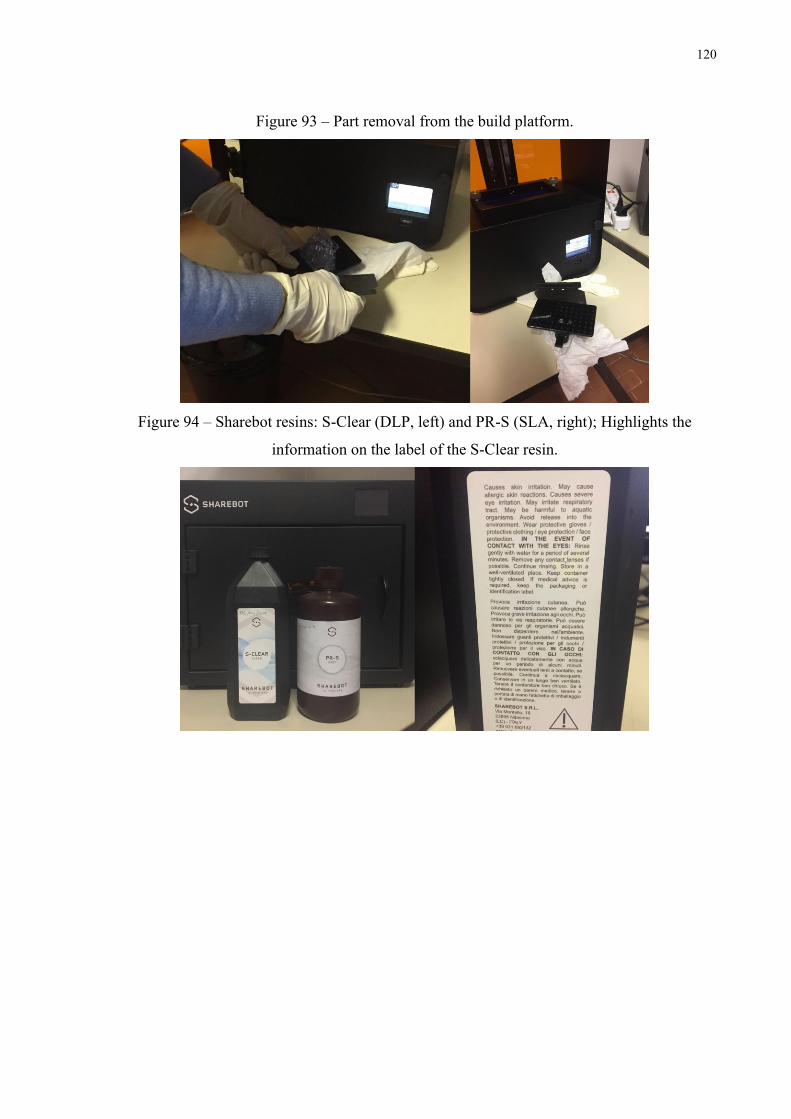
120

Figure 93 – Part removal from the build platform.

Figure 94 – Sharebot resins: S-Clear (DLP, left) and PR-S (SLA, right); Highlights the

information on the label of the S-Clear resin.

121

II. SHAREBOT ANTARES – SLA MANUFACTURING

Figure 95 – Opened Sharebot Antares and preparison; Highlights platform and establishes a

reference of size (screw).

Figure 96 – Sharebot Antares interior during fabrication; Highlights the current UV curing

point whilst referring to a reference of size (screw).

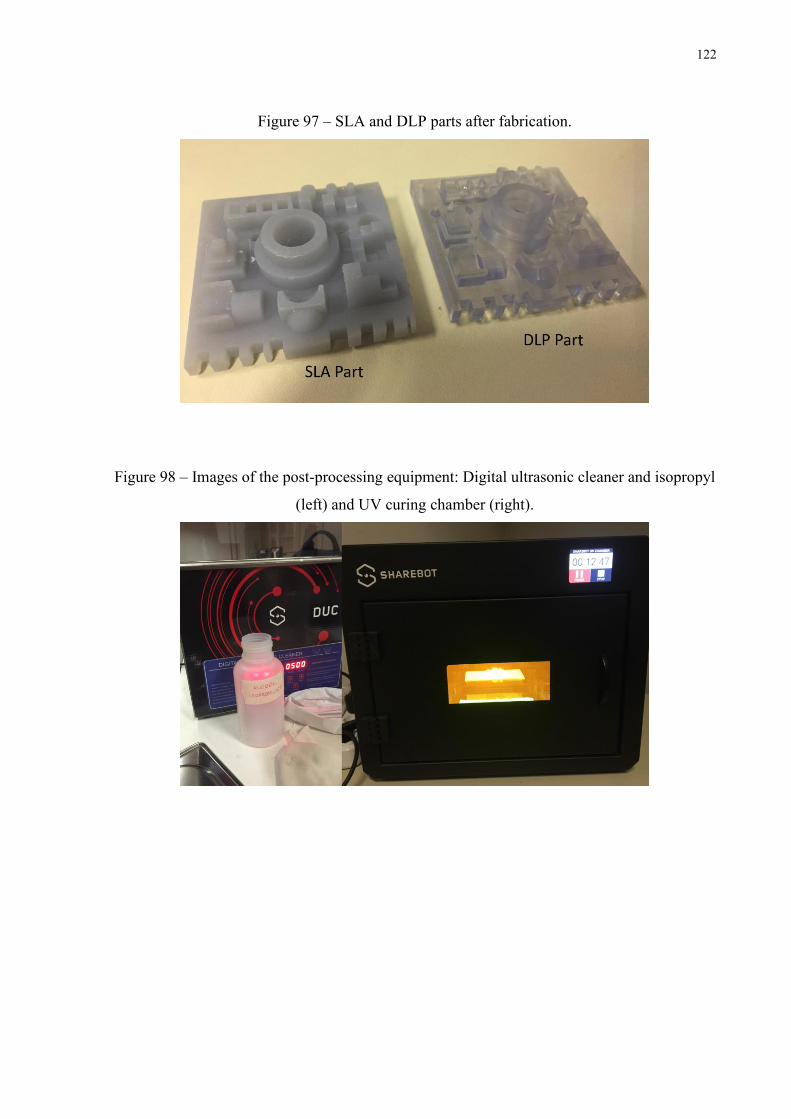
122

Figure 97 – SLA and DLP parts after fabrication.

Figure 98 – Images of the post-processing equipment: Digital ultrasonic cleaner and isopropyl

(left) and UV curing chamber (right).

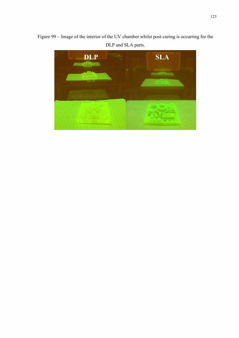
123

Figure 99 – Image of the interior of the UV chamber whilst post-curing is occurring for the

DLP and SLA parts.

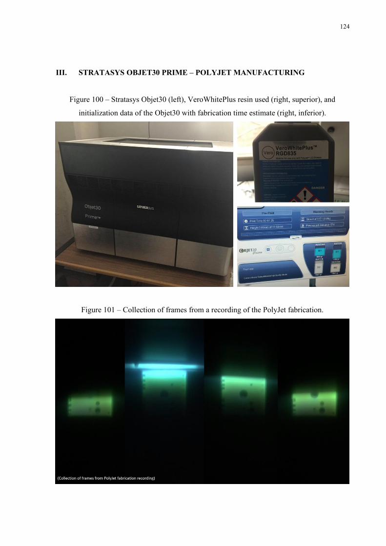
124

III. STRATASYS OBJET30 PRIME – POLYJET MANUFACTURING

Figure 100 – Stratasys Objet30 (left), VeroWhitePlus resin used (right, superior), and

initialization data of the Objet30 with fabrication time estimate (right, inferior).

Figure 101 – Collection of frames from a recording of the PolyJet fabrication.

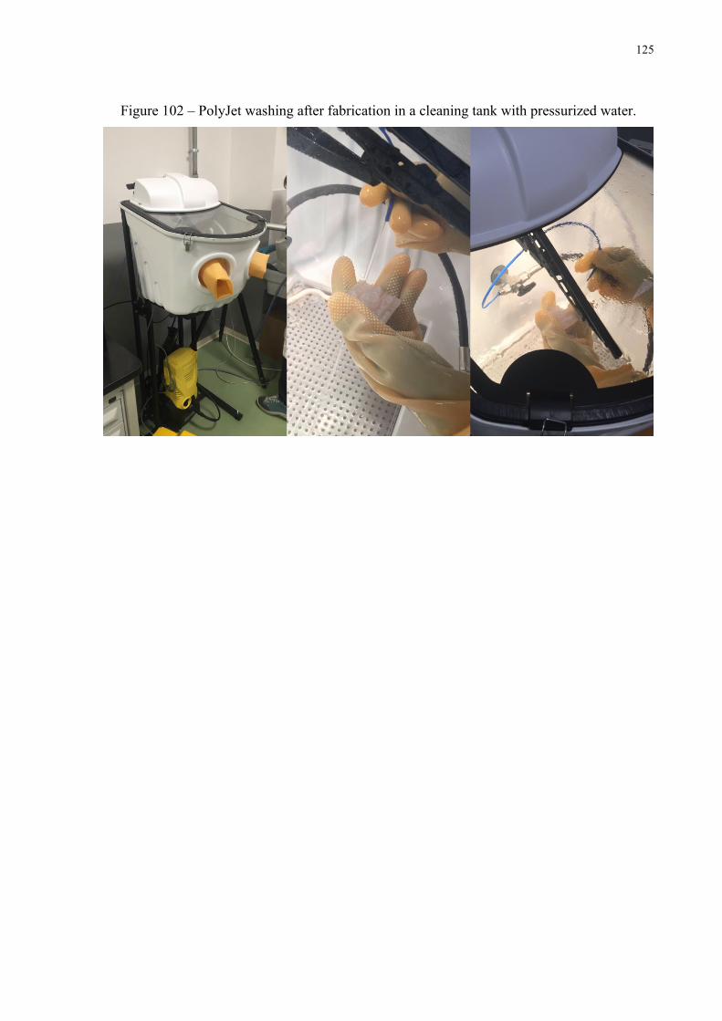
125

Figure 102 – PolyJet washing after fabrication in a cleaning tank with pressurized water.

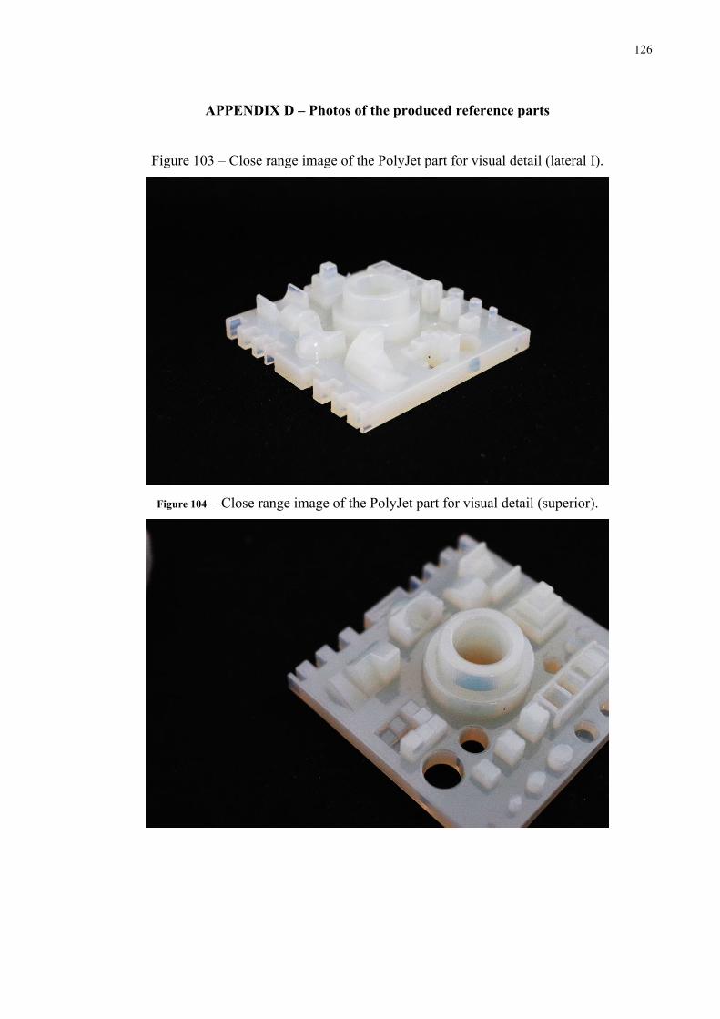
126

APPENDIX D – Photos of the produced reference parts

Figure 103 – Close range image of the PolyJet part for visual detail (lateral I).

Figure 104 – Close range image of the PolyJet part for visual detail (superior).

127

Figure 105 – Close range image of the PolyJet part for visual detail (lateral II).

Figure 106 – Close range image of the PolyJet part for visual detail (lateral III).

128

Figure 107 – Close range image of the PolyJet part for visual detail (lateral IV).

Figure 108 – Close range image of the DLP part for visual detail (lateral IV).

129

Figure 109 – Close range image of the SLA part for visual detail (lateral IV).

POLITECNICO DI TORINO DEPARTMENT OF MANAGEMENT AND ...

Documents

Transcript of POLITECNICO DI TORINO DEPARTMENT OF MANAGEMENT AND ...