
POLITECNICO DI TORINO DEPARTMENT OF CONTROL AND …
87
POLITECNICO DI TORINO DEPARTMENT OF CONTROL AND COMPUTER ENGINEERING MASTER’S DEGREE IN COMPUTER ENGINEERING Master’s Degree Thesis: A Data Compression Approach for Big Data Classification Supervisor: Professor Paolo Garza Candidate: Eskadmas Ayenew Tefera ID – 236174 December 2020
Transcript of POLITECNICO DI TORINO DEPARTMENT OF CONTROL AND …

POLITECNICO DI TORINO
DEPARTMENT OF CONTROL AND COMPUTER
ENGINEERING
MASTER’S DEGREE IN COMPUTER ENGINEERING
Master’s Degree Thesis: A Data Compression Approach for Big
Data Classification
Supervisor:
Professor Paolo Garza
Candidate:
Eskadmas Ayenew Tefera
ID – 236174
December 2020

2
A Data Compression Approach for Big Data Classification
Abstract
By Eskadmas Ayenew Tefera
Politecnico di Torino
Supervisor: Professor Paolo Garza
A data compression approach for big data classification is important, to compress large size
dataset into small and manageable dataset, then to create and build the classification model for
the compressed dataset and evaluate the model’s accuracy. Data compression algorithms are
used to compress and reduce the size of dataset. The compression mechanisms help to increase
and optimize operational efficiencies, enable cost reductions, and reduce risks for the business
operations. It is becoming costly to process large size datasets. The compression algorithm
controls each bit of a dataset and optimizes the size without losing any data, by using a lossless
data compression approach. In a lossless data compression, data can be compressed without
loss. Therefore, the restored dataset is equal to the original form of the dataset.
In this thesis, a classification model for the initial datasets has been created and built by using
a J48 classification algorithm. The built-in model of the original datasets has been evaluated to
get the evaluation statistics of the model, the accuracy of the model, and the confusion matrix
results of the model. Then, it is possible to extract correctly and incorrectly classified instances
of a given dataset. The built-in decision tree has root, internal, and leave nodes, which draws
paths of the tree. A path is a way from the root-through-internal-to-leave node and the number
of paths are equal to the number of leaves. In each path, there are one or more instances. We
can extract the paths of correctly and incorrectly classified instances from the classifier model.
In addition, it is also possible to extract instances from the paths. In order to get paths of the
tree and an instance from a path, it is required to generate and get the source strings of the tree.
We can extract instances from the tree or from each path and create a compressed small dataset.
Then we can concatenate one compressed dataset with the other compressed dataset and create
another compressed dataset. Like the original dataset, we created and built classification
models for the compressed datasets. The models have been evaluated and the evaluation results
of the compressed dataset model have been compared with the evaluation results of the original
dataset model. As a result, we can see the accuracy of the classification models of the original
and compressed datasets. The initial datasets have been selected from UCI Machine Learning
Repository.

3
Acknowledgement
First and foremost, I want to thank the almighty God, for always helping me and giving
me the patience to deal with everything. Next, I would like to express my sincere appreciation
and gratitude to my supervisor, Professor Paolo Garza, for his guidance and invaluable
comments during doing this thesis. In addition, I would like to thank my dear wife Dr. Senay
Semu, for her support and encouragement throughout this study. Finally, I would like to thank
our families and friends for their continuous encouragement and appreciation.
Eskadmas Ayenew Tefera

4
Table of Contents Chapter One ………………………………………………………………………………….. 6
1. Introduction …………………………………………………………………………... 6
1.1.Overview of Big Data Classification …………………………………………………. 6
Chapter Two ...………………………………………………………………………………... 9
2. Review of Related Literature ……………………………………………………….... 9
2.1. Big Data ……………………………………………………………………………... 9
2.2. Big Data Analytics ………………………………………………………………… 13
2.3. Classification Algorithms ………………………………………………………….. 16
2.4. Decision Tree Algorithms …………………………………………………………. 19
2.5. WEKA Library …………………………………………………………………….. 24
2.6. Data Compression for Big Data …………………………………………………… 27
Chapter Three ………………………………………………………………………………. 30
3. Developing Decision Tree Model and Extract Information ………………………... 30
3.1. The Addressed Problem ………………………………………………………….... 30
3.2. The Proposed Solution …………………………………………………………….. 31
3.3. Preparing the Dataset ………………………………………………………………. 35
3.4. Pre-processing the Dataset ………………………………………………………… 37
Chapter Four ………………………………………………………………………………... 54
4. Experimental Results ……………………………………………………………….. 54
Chapter Five ………………………………………………………………………………... 84
5. Conclusions and Future Work ……………………………………………………… 84
5.1. Conclusions ………………………………………………………………………... 84
5.2. Future Work ……………………………………………………………………….. 85
References ………………………………………………………………………………….. 86

5
List of Figures 1. The 3V’s of Big Data ………………………………………………………………... 10
2. The 5V’s of Big Data ………………………………………………………………... 11
3. Big Data Analytics ………………………………………………………………….. 14
4. The Importance of Big Data Analysis ……………………………………………….. 14
5. Oracle Big Data Solution ……………………………………………………………. 16
6. Nodes in a Decision Tree ……………………………………………………………. 21
7. WEKA Implementation …………………………………………………………….. 24
8. File Formats Supported in WEKA …………………………………………………... 26
9. Example of an ARFF File …………………………………………………………… 26
10. Classifier, Test Options, and Classifier Output in WEKA Explorer ………………… 32
11. Car.arff Dataset in WEKA Explorer ………………………………………………… 38

6
Chapter One
Introduction 1.1. Overview of Big Data Classification
In the present days, companies are realizing the importance of using large set of data to support
their decisions and develop strategies. They are investing more in processing large set of data
rather than investing more in expensive algorithms. Because a larger amount of data gives
better information on the ongoing trends. Nowadays, we are living in an informational society
and moving towards a knowledge-based society. A large amount of data on a specific case is
required to extract better knowledge on that case. As we can see in our day-to-day life,
information plays the key role in economy, politics, and cultural aspects of the society. The
competitive advantage that companies gained is through understanding the available data and
predicting the progress of facts based on the data at hand. Organizations collect a large set of
data and analyzes it to extract correlations and support their decisions. However, big data
analytics is a challenging and complex task.
Data compression is required for reliable and timely retrieval of information. Data compression
processes and programs have developed to address the difficulty of processing large volume or
complex data. Data compression reduces the size of data to a certain level and minimize the
operational time of fetching the records from the data warehouse. Compression techniques are
used to convert data from an easy-to-use presentation to one enhanced for compactness while
uncompressing techniques are used to return the data to its original form. Data compression
techniques are used on very large data in logical and physical databases.
Nowadays, big data analytics and data mining are the main research areas. Big data
classification is one of the main concerns in data mining. Classification refers the decision or
prediction that has been made on the basis of currently available knowledge or information.
Classification algorithms are used to make predictions and applied to classify objects that are
previously uncover. Each newly classified object is assigned to a class that is belonging to a
predefined set of classes. Classification algorithms analyse datasets in a supervised or
unsupervised way. There are two main steps in supervised classification process. These are –
the training step where the classifier model is built and the classification step that applies the
trained model to assign unknown data to one out of a given set of class labels. Classification
algorithms construct the model based on learning rules from examples. In this thesis, J48

7
classification algorithm of the WEKA interface has been used to do all the experiments. J48 is
a Java implementation of C4.5 algorithm. It induces classification rules in the form of decision
trees for a set of given instances. Decision trees are the approaches to represent classifiers.
Decision tree is a classifier described as a recursive partition of records of a dataset. It consists
of different nodes that form a rooted tree, which is a directed tree with a ‘root’ node that has
no incoming edges.
The decision tree models of the datasets have created by using Java programs that use WEKA
libraries. WEKA (Waikato Environment for Knowledge Analysis) is a well known suite of
machine learning that is a software written in Java. The WEKA suite provides a collection of
visualization tools and algorithms for data analysis and predictive modeling. It has also
graphical user interface (GUI) to easily access its functionality. WEKA enables to do several
standard data mining tasks, such as – data preprocessing, clustering, classification, regression,
visualization, and feature selection. The implementation of a specific learning algorithm in
WEKA, is encapsulated in a class. This learning algorithm may use other classes to do some
of its functionalities. An algorithm creates an instance of this class through allocating memory
for a decision tree classifier to be built. This is done each time when the Java virtual machine
(JVM) executes J48 class. The classifier model, the algorithm, and a procedure for outputting
the classifier are all part of the instantiation of the J48 class. The program will split into two or
more classes if it is larger. It includes references to instances of other classes, which perform
most of the tasks. [1]
The rest of the thesis is organized in the following way.
Chapter two discusses about the reviews of related literature. We tried to look other related
researches and documentations to enrich this thesis. As a result, chapter two has discussed
about which other related researches have discussed about the key concepts found in this thesis.
More specifically, this chapter describes about big data, big data analytics, classification
algorithms for big data, decision tree algorithms, WEKA libraries, and data compression for
big data.
Chapter three discusses about the problems that this thesis has tried to address, and the designed
methodologies developed to address the problems. It describes about the required things in this
thesis (statement of the problem), the datasets to be used for the experiments, how to prepare
and pre-process the datasets to make them ready for processing. Moreover, chapter three

8
discusses about the designed methodologies to address the problems and the proposed solutions
by this thesis. The designed methodologies are the Java programs that are developed based on
WEKA, which can do various classification tasks of J48 classification algorithm.
In chapter four, it has discussed about the experimental results of the designed methodologies
and the analysis of the experimental results. In addition, it describes general information of the
datasets used in the experiments.
Chapter five discusses about the conclusions of the work done in this thesis and about the future
works proposed for further researches.
The datasets used for the experiments have been chosen from UCI Machine Learning
Repository.

9
Chapter Two
Reviews of Related Literature 2.1. Big Data
The term “Big Data” is used to define a large amount of data that can’t be managed and
processed by traditional data management techniques due to its complexity and size. This term
was introduced to the computing world in 2005 [2]. Studies have shown that the term “Big
Data” was used in researches since 1970s. However, it was introduced in publications to the
computing world in 2008. [3]
The Gartner’s IT Glosarry defines big data as high volume, high velocity, and high variety of
information assets, which require cost-effective and innovative forms of information
processing. The processed information is used for enhanced insight, decision making and
process automation. Big data refers to structured or unstructured large sets of complex data;
traditional data processing techniques or algorithms are unable to operate it. [4] It aims to reveal
hidden patterns and led to an evolution from a model-driven to data-driven science paradigm.
Big data rests on the interplay of the following concepts. [4]
a. Technology – maximizing computational power and algorithmic accuracy to gather,
analyze, link, and compare large datasets.
b. Analysis – drawing on large datasets to identify patterns to make economical, social,
technical, and legal claims.
c. Mythology – the widespread belief that large datasets provide a better intelligence
and knowledge, which can enable to generate insights that were previously unseen,
with the goal of truth, objectivity, and accuracy.
Big data is a field of study that provides ways to analyze data, systematically extract
information from large set of data, or deal with datasets that are too large or complex to be
dealt with by traditional data-processing applications. It also refers extremely large datasets
that are analysed computationally to discover patterns, trends, and associations, which are
relating to human behaviour and interactions. Nowadays, the concept of big data is treated from
different points of view and referred in different fields.

10
Big data is described by its size, which consists of large, complex, and independent collection
of data. These independent datasets may interact with each other. The possible integration of
the independent parts of the dataset might be inconsistent and unpredictable. Therefore, it might
be impossible to handle big data by using standard techniques of data management. [5]
The term "big data" is also refers to the growth and usage of technologies that are used to
provide the right information, at the right time, to the right user, from a mass of data. The
challenge includes to deal with rapidly increasing volumes of data, managing increasingly
heterogeneous formats, increasingly complex, and interconnected data. Big data is a complex
polymorphic object. It is invented by the giants of the web and designed to provide a real-time
access to giant databases. Big data refers larger volume datasets, more diversified, including
(structured, semi-structured, and unstructured data (variety)), and accessed faster (velocity). It
includes the 3Vs. [6]
Big data was originally associated with three key concepts: volume, variety, and velocity.
Fig. 1. 3V Concept [6]
According to IBM scientists, big data has four-dimensions – Volume, Velocity, Variety, and
Veracity [7].
Volume – refers to the quantity of data gathered through different mechanisms. This data is
required to get the necessary information or knowledge. Companies gather data from various
sources such as business transactions, Internet of Things (IoT) devices, archived videos, social
media, etc. In the past, it was difficult to store these data. The cheaper technologies for big data
storage such as Hadoop and data lakes have resolved this problem. The cloud technologies
have provided the option to store large datasets remotely.

11
Velocity – refers the time that takes to process big data. Fast processing maximizes efficiency,
which is required for activities that are very important and need immediate responses. With the
growth in the Internet of Things (IoT), data streams into businesses at an unprecedented speed
and require to be handled timely. Data can be collected in real-time through RFID (Radio-
frequency Identification) tags, sensors and smart meters.
Variety – refers to the type of data that big data can comprise. This data can be structured as
well as unstructured. In traditional databases data is found in structured and numeric formats.
Data is also found in formats like unstructured text files, emails, videos, audios, stock
transactions and other financial transactions.
For this classical characterization, two other "V"s are included [6]
Fig. 2. 5V Concept [6]
Veracity – the user needs to trust the extracted information to take decision based on it.
Veracity refers the degree to which the user trusts the result of data analytics. Getting the right
correlations in big data is vital for the future of the business.
Value – the value and potential gained from big data.
The challenges of big data occur in collecting, storing, analyzing, searching, querying,
visualizing, updating, sharing, and transferring of big data. Assuring its privacy and confirming
its source are also the other challenges. During handling big data, the handler may not sample
rather it simply observe and track what happens.
According to Ed Dumbill, big data is defined as the data that exceeds above the processing
capacity of conventional database systems. [8] The data is too big, moves too fast, or doesn’t
fit with the structures of our database architectures. It requires to choose an alternative way to
process big data in order to gain value from it.

12
Big data also refers the large and diverse sets of data that grow at ever-increasing rate. It
involves the volume of data, the velocity that it is created or collected, and the variety of the
data points being covered. Big data often comes from multiple sources like Oracle, Postgres,
Hadoop, Mango, etc., and arrives in multiple formats like JSON, string, CSV, etc. Big data can
be categorized as structured or unstructured data. An organization handles information in
databases and spreadsheets, which is structured data. While unstructured data is unorganized
and do not found in a preknown model or format. Big data is usually stored in computer
databases and processed by using softwares, which are particularly designed to handle huge
and complex datasets. Companies that provide Software-as-a-Service (SaaS) are managing this
type of large and complex data. [9]
In big data processing, improving the efficiency of data handling, is the main goal to achieve.
If big data is processed properly and used accordingly, organizations can get a better view on
their business. This increases the efficiency of an organization. [2]
Big data is used in various fields. [2]
• In information technology – analyzing the patterns from the existing logs (i.e. large log)
enables to improve security and troubleshooting of the system.
• In customer service – it is used to get the customer pattern and enhance customer
satisfaction of services by analyzing information from call centers.
• To improve services and products through the use of social media information. It
enables to know the preferences of potential customers and modify its product.
• To detect fraud in online transactions for any industry.
• In risk assessment – by analyzing the transaction information.
Big data generally refers to data that exceeds the storage, processing, and computing capacity
of conventional databases. As a result, it requires advanced data analytics techniques, tools and
methods to analyze the large dataset, extract patterns from large-scale dataset, and get the
required information or knowledge from them. [10]

13
2.2. Big Data Analytics
Big data analytics is the strategy of analyzing large volumes of data, which are gathered from
various sources, such as – social networks, digital images, sensors, sales transaction records,
etc. It aims to uncover patterns and connections that might be invisible and provide valuable
information. As a result, businesses may be able to gain an advantage over their rivals and
make superior business decisions. [11] Big data analytics is one of the challenging processes
in scrutinizing big data to acquire the required information that is important for an organization
to support their business decisions. In this digital era, data is a nitty-gritty to gain insights that
are essential for business.
Big data analytics is the process of analyzing very large and diverse datasets by using advanced
analytic techniques. These datasets may be structured, semi-structured and unstructured data,
which are collected from different sources and they are in different sizes from terabytes to
zettabytes [12]. The analysis of big data provides previously inaccessible or unusable data,
which allow analysts, researchers and business owners to make better and faster decisions.
Businesses can use advanced analytics techniques to gain new insights from previously
untapped data sources independently or together with existing enterprise data. The techniques
include – text analytics, machine learning, predictive analytics, data mining, statistics and
natural language processing. Big data analytics enables data scientists and other users to
analyze large volumes of transaction and other raw data, which can’t be handled by traditional
business systems. Traditional systems are unable to analyze large data sources, which may fall
short [13]. Big data analytics is done by sophisticated software programs, but the unstructured
data used in analytics may not be well suited to conventional data warehouses.
Big data needs high processing requirements that may make traditional data warehousing a
poor fit. As a result, the newer and bigger analytics environments and technologies have
emerged. These are – Hadoop, MapReduce and NoSQL databases. These technologies used an
open – source software framework to process huge datasets over clustered systems. When we
combine big data with analytics, it provides new insights that can drive digital transformation.
For example, big data helps insurers to better assess risks, create new pricing policies, make
highly personalized offers and be more proactive about loss prevention.
In general, big data analytics evaluates large datasets to discover hidden patterns, correlations
and the required insights. The analytics helps organizations to analyze the data they have and
finds new business opportunities. This leads to smarter and effective business moves, more
efficient operations, higher profits and address customers’ needs.

14
The following picture shows how big data works in converting unstructured data and analyzes
it. [9]
Fig. 3. Big data analytics [9]
As it has discussed previously, big data analytics includes the whole process of evaluating large
datasets through various analytics tools and processes the data to get unseen patterns, hidden
correlations, significant trends, and other insights used for making data-driven decisions in the
aim of better results.
Big data analytics uses a set of technologies and techniques, which require new forms of
integration to extract hidden values from large datasets. The extracted values are different from
the initial ones, which are more complex and in a large enormous scale. The analytics use better
and effective ways to mainly solve new or old problems.
Fig. 4. The importance of big data analysis [14]

15
1. Cost reduction – in storing large amounts of data as well as identifying more efficient ways
of doing business, big data technologies such as Hadoop and cloud-based analytics have
brought significant cost advantages.
2. Faster, better decision making – businesses can get information faster and make decisions
based on what they’ve experienced. This is gained by implementing Hadoop and in-memory
analytics together with the ability to analyze new sources of data.
3. New products and services – it enables to provide what the customers want. With big data
analytics, more companies are creating new products to meet customers’ needs.
Types of Big data Analytics [6]
a) Descriptive analytics – it deals with what is happening?
It is a preliminary stage of data processing that creates a set of historical data. Data analytics
mechanisms manage data and discover hidden patterns that give insight. Descriptive analytics
provides future probabilities or trends and gives an idea about what might happen in the future.
b) Diagnostic analytics – it deals with why did it happen?
Diagnostic analytics examine the root cause of a problem, which is used to determine why and
how the problem has happened. This type of attempt is used to find and understand the causes
of events and behaviors.
c) Predictive analytics – it deals with what is likely to happen?
It uses past data to predict the future. It is all about forecasting. Predictive analytics uses data
mining and artificial intelligence techniques to analyze current data and make analysis about
what might happen in the future.
d) Prescriptive Analytics – it deals with what should be done?
It intends to find the right measure to be taken. Predictive analytics helps to forecast what might
happen by using historical data provided by descriptive analytics. Prescriptive analytics finds
the best solution through using these parameters.
The following are the dimensions at which big data analytics is different from traditional data
processing architectures.

16
• Decision makers worry about the speed of decision making
• The data processing task is complex
• The volume of transactional data is very huge
• Data can be found in structured or unstructured form
• Flexibility of processing (analysis)
• Concurrency
Big data analytics is a joint project of both information technology (IT) and business. IT
deploys the right big data analysis tools and implementing data management practices. Both
targets the value added by business improvements that are brought about by the initiative. [2]
Fig 5. Oracle Big data Solution (Source: myoracle.com)
2.3. Classification Algorithms
Classification in machine learning is defined as the process of predicting class or category from
observed values or given dataset. The categorized output can have the form such as – “black”
or “white”, “spam” or “no spam”, etc. The training dataset is required to get better boundary
conditions, which are used to determine each target class. After determining the boundary
conditions, the next task is to predict the target class. The whole process is called classification.
Classification includes two steps, which are learning step and prediction step. In learning step,
the model has been developed through a given training dataset while in the prediction step, the
model is used to predict the response for given data.
Classification is the main topic in machine learning, which trains the machine on how to
classify data by using a given criteria. It is the process by which machines group data together

17
based on predefined characteristics, which is called supervised learning. Whereas in
unsupervised classification that is also called clustering, machines find shared characteristics
to group data when categories are not specified.
There are two main steps in the supervised classification process. The first step is the
training step, where the classification model is built. The second step is the classification
itself, which applies the trained model to assign unknown data to one out of a given set of class
labels. Detecting spam emails is a common example of classification. The training model is
created and built by a dataset that has both spam and non-spam emails. The developed program
can identify spam emails. An algorithm can learn the characteristics of spam emails from the
training dataset. Then it can filter out spam emails when it encounters new emails.
Classification is simply grouping things together based on their similar features and attributes.
It is required to choose the right classification algorithm to build a model. A classifier is an
algorithm that performs classification. The classifier algorithm should be accurate and fast. It
sometimes reduces the size of training data to the size that it requires. If the dataset has more
parameters, the train set for an algorithm must be larger. Classification algorithms have
different ways of learning patterns. [15]
The following are the basic terminologies in classification algorithms.
o Classifier – is an algorithm that maps an instance of the dataset to a particular category
o Classification model – it draws conclusion from the instances of the training dataset. It
predicts the class labels for every new instance.
o Feature – is a measurable property of a phenomenon being observed.
o Binary classification – it is a classification task with two possible results.
Example – Male / Female, True / False, Correct / Incorrect
o Multi-class classification – refers classifying an instance with more than two classes.
In multi-class classification, each instance is assigned to one and only one target label.
Example – a course can be a SE or BD but not both at the same time.
o Multi-label classification – is a classification task, each instance is mapped to a set of
target labels (more than one class).
Example – a food can be pizza, cake, and bread at the same time.

18
Classification algorithms are broadly categorized as the following:
• Linear Classifiers – example: logistic regression, naive bayes classifier
• Support Vector Machines (SVM)
• Quadratic classifiers
• Kernel estimation – example: k-nearest neighbor
• Decision trees
• Neural networks
• Learning vector quantization
Logistic Regression – is a supervised learning classification algorithm, which is used to predict
the probability of a target variable. The nature of target or dependent variable is dichotomous,
which means there would be only two possible classes.
Naive Bayes Classifier – it assumes that the presence of a specific feature in a class is not
associated with the presence of any other feature. For example, if a fruit is round, red, and about
3 inches in diameter, it may be considered to be an apple.
Decision Trees – Decision tree analysis is a predictive modelling tool that can be constructed
by an algorithmic approach to split the dataset in various ways. The split is done based on
different conditions. Decision trees are the mostly used classification algorithms, which are
categorized under supervised algorithms.
KNN (k-Nearest Neighbors) – KNN algorithm is categorized under supervised machine
learning algorithm, which can be used for both classification and regression predictive
problems. However, it is mainly used for classification predictive problems. It uses ‘feature
similarity’ to predict the values of new data points, which further means that the new data point
will be assigned a value based on how closely it matches the points in the training set.
SVM (Support Vector Machine) – SVMs are a powerful and flexible supervised machine
learning algorithms, which are used both for classification and regression. But generally, they
are used in classification problems that can handle multiple continuous and categorical
variables.

19
Classification Problems Classification is a classical problem in machine learning. [16] Classification problem refers the
most common prediction problem. The data has a dependent variable, which has clear-cut of
distinct categories that the model needs to predict. Most of the algorithms learn a function to
come up with a decision boundary, which helps in classifying the data and providing them with
separate class labels. The ‘settings’ of the algorithms are often constantly ‘updated’ and various
techniques are used to reduce the errors where an error is a misclassification, which means
assigning a wrong data label to a data point. [15]
The most commonly used performance metrics for classification problem are – accuracy,
confusion matrix, precision, recall, ROC AUC, Log-loss, etc. Accuracy refers the ratio of the
number of correctly classified instances with the total number of instances of the dataset.
Confusion matrix is a summary of predicted results in a table, which visualizes the performance
measure of the machine learning model for a binary classification problem (2 classes) or multi-
class classification problem (more than 2 classes). Precision and recall are the fraction of the
correctly classified instances from the total classified instances. The ROC curve is generated by
plotting the cumulative distribution function of the True Positive in the y-axis versus
the cumulative distribution function of the False Positive on the x-axis.
2.4. Decision Tree Algorithms
Decision tree is a popular classification algorithm, which is easy to understand and interpret. A
decision tree analysis is a predictive modelling tool, which aims to classify the dataset based
on the required criterion. Decision trees are built by an algorithmic approach, which are the
most powerful algorithms categorized in supervised learning algorithms. They are used both
for classification and regression operations. A tree has two main entities, which are decision
nodes where the data is split and the leaves where we get the outcome (i.e. class).
Decision tree is a classification technique that is described as a recursive partition of the
instance space. It contains nodes that form a rooted tree, which is a directed tree with a ‘root’
node. The root node has no incoming edge, but it has outgoing edges. While all other nodes
have exactly one incoming edge. Internal or test nodes have both incoming and outgoing edges.
Leaf nodes are also called terminal or decision nodes, which have no outgoing edges. Based
on a certain discrete function of the input attributes values, each internal node splits the instance
space into two or more subspaces in a decision tree. An instance has grouped based on an

20
attribute’s value and every test evaluates a single attribute. The condition will be a range for
numeric attributes.
A class label is given for each leaf that represent the most appropriate target value. The leaf
holds a probability vector, which is the probability of the target attribute that have a given
value. Based on the outcome of the tests in the path, instances are classified by navigating them
from the root of the tree down to the leaf. A decision tree comprises both numeric and nominal
attributes. The dataset analyst can predict the response of a customer by sorting it down the
tree. It is possible to understand the behavioral characteristics of the entire population. Each
node is labeled with an attribute that it tests and the branches of a node are labeled with its
corresponding values. [17]
A decision tree algorithm is categorized in the supervised learning algorithms. It can be used to
perform regression and classification processes. A decision tree creates a classifier model to
predict the class or value of the target variable by learning decision rules from the training
dataset. In decision trees, the process starts from the root of the tree to predict a class label for
an instance of the dataset. Then it compares the values of the root attribute with the instance’s
attribute. It follows the branch corresponding to that value and jump to the next node, based on
the comparison results.
Types of Decision Trees
The types of decision trees based on target variable:
1. Categorical variable decision tree – the decision variable is categorical.
2. Continuous variable decision tree − the decision variable is continuous.
The types of nodes of the decision tree:
1. A root node – it has no incoming edges, and it has zero or more outgoing edges. It
represents the entire population or sample and it is further divided into two or more
homogeneous sets.
2. Internal nodes – have exactly one incoming edge and two or more outgoing edges.
3. Leaf (terminal) nodes – have exactly one incoming and no outgoing edges. They do
not split anymore.

21
Root node represents the entire dataset or a sample of the dataset. Splitting is the process of dividing
a node into sub-nodes. Decision node is a sub-node that splits into other sub-nodes. Leaf or
terminal nodes are nodes that do not further split. Pruning is the process of deleting sub-nodes
of a decision node and it is the opposite of splitting. Branch or sub-tree is the sub-part of the entire
tree. A parent node is a node that is divided into sub-nodes. The parent node’s sub-nodes are called
child nodes. [18]
Fig.6. Nodes in a decision tree [18]
Decision trees classify the records of a dataset through sorting them down to the tree, starting
from the root node to the leaf (terminal) node or nodes. The leaf node enables classification of
the dataset. Each node acts as a test case for some attribute and each edge descending from the
node corresponds to the possible answers to the test case. This process has been done in a
recursive way and is repeated for every sub – tree rooted at the new node.
Things to be considered when creating a decision tree:
• First, the whole training dataset is considered as the root.
• The feature values are preferred to be categorical.
Continuous feature values need to be discretized on top of building the model.
• On the basis of their attribute values, instances are distributed recursively.
• Attributes are placed at the root or at the other levels based on their statistical values.

22
Identifying an attribute used as a root node and at each level, are the main challenges in decision
tree implementation. The process of handling this condition is called attributes selection process.
There are various attributes selection measures in order to identify the attribute that can be used
as a root node at each level.
Decision trees work in the following way
The decision of performing strategic split highly affects the tree’s accuracy. Classification and
regression trees have different decision criteria. The decision tree algorithms decide to split a
node into two or more sub-nodes. When sub-nodes created, it increases the homogeneity of
resultant sub-nodes. A node’s purity increases with regard to the target variable. The decision
tree algorithm splits the nodes by the available variables and selects the split that results in most
homogeneous sub-nodes. An algorithm selection is based on the type of target variables. [18]
The following are the algorithms used in decision trees.
ID3 – it is an extension of D3. The ID3 algorithm builds decision tree by using a top-
down greedy search approach through the space of possible branches with no backtracking. A
greedy algorithm always makes the choice that seems to be the best at that moment.
C4.5 – it is the successor of ID3
CART (Classification And Regression Tree)
CHAID (Chi-square Automatic Interaction Detection) – it performs multilevel splits during
computing classification trees.
MARS (Multivariate Adaptive Regression Splines)
The following are the steps in ID3 algorithm [18]
1. The algorithm starts with the original set S as the root node.
2. It iterates on unused attribute of the set. For each iteration, it calculates information gain
and entropy of an attribute.
3. It selects an attribute that has the smallest entropy or largest information gain.
4. The set is split by the selected attribute to produce a subset of data

23
5. The process continues on each subset by considering the attributes never selected before.
Attribute Selection Measures
The dataset has N number of attributes. Deciding to place an attribute at the root or at the other
levels of the tree, as internal and leaf nodes, is a challenging task. Randomly selecting any node
and make it the root node can’t solve the case. A random approach may give us bad results with
low accuracy. Researchers have studied and proposed some solutions to solve attribute selection
problems. They suggested to use the criterion such as – Entropy, Information gain, Gini index,
Gain Ratio, Reduction in Variance, and Chi-Square. They calculate values for every attribute
and the values are sorted. The attributes are placed in the tree through following the order, an
attribute with a high value (in information gain) is placed at the root. For attributes assumed to
be categorical, Information Gain will be used as a criterion. For attributes assumed to be
continuous, Gini index will be used as a criterion. [18]
In a decision tree, each leaf node is assigned a class label. The root and other internal nodes are
non-terminal nodes, which contain attribute test conditions. This is used to separate records
that have different characteristics. Once a decision tree has been constructed, classifying a test
record is straightforward. Starting from the root node, the test condition is applied to the record
and follow the right branch-based outcome of the test. This lead either to another internal node,
for which a new test condition is applied, or to a leaf node. The class label associated with the
leaf node is then assigned to the record.
The steps to make a decision tree are: [19]
1. Decide which split to make. Try every split and choose which one seems best according
to the splitting criteria used by the algorithm.
2. Make this split and choose which class to give to both parts of the split. The class chosen
is the class that most of the observations in this part belong to.
3. For each subset, make a new split in the same way. Order in which to split these subsets
is irrelevant, as they will all have to be looked at.
4. Repeat this until some stopping criteria is met. This can be the depth of the tree or the
amount of observations left in a node.
5. Depending on the algorithm, pruning is used at the end.

24
For pruning, delete a part of the tree and see if this make the tree better. The way to measure
how good the tree is, differs per algorithm.
2.5. WEKA Library
WEKA was developed at the university of Waikato in New Zealand. The name stands for
Waikato Environment for Knowledge Analysis. WEKA pronounced to rhyme with Mecca, is
a flightless bird with an inquisitive nature found only on the islands of New Zealand [20].
WEKA is written in Java and runs on every platform such as – Linux, Windows, and Macintosh
operating systems. WEKA is the library of machine learning, which is used to solve various
big data analytics problems. The system allows implementing various algorithms to extract
data and call algorithms from various applications using Java programming language.
WEKA is an open source software that comprises the tools that are used for preprocessing the
dataset, implementing various machine learning algorithms, and visualization purposes. It
provides machine learning techniques to be applied on data analytics problems. [21]
Fig. 7. WEKA implementation [21]

25
At the beginning, we start with the raw data that contain several null values and irrelevant
fields. We can clean the data by using the data processing tools, which are provided by
WEKA. Then save the preprocessed data into the local storage and apply machine learning
algorithms on it. Depending on the model to be developed, we can select one among the
options like Classify, Cluster, or Associate, etc. In order to create a reduced dataset, an
attribute selection process allows an automatic selection of features.
In each category, WEKA provides the implementation of several algorithms. We can select an
algorithm that we want to use, set the desired parameters, and start to run. As a result, WEKA
provides the statistical output of the model processing as well as a visualization tool to inspect
the data. The same dataset can be processed by various models. It can be possible to compare
the outputs of different models and select the best one. WEKA enables to develop machine
learning models in a fast and easy way. It includes a set of features for the operations such as
– data processing, classification, clustering, regression, association rule creation, feature
extraction, and visualization. WEKA is an efficient data analytics tool that allows to develop
new approaches in the field of machine learning. WEKA provides direct access to the library
of implemented algorithms. This feature makes it possible to apply algorithms created in
different systems based on Java. [22]
In WEKA, learning algorithms can be applied to the datasets. It includes tools to transform
datasets, like the algorithms used for discretization and sampling. It enables to preprocess the
dataset, load to the learning scheme, analyze the classifier results and its performance; all these
can be done without writing any program code. To learn more about the data, it is required to
apply a learning method to a dataset and analyze the result. The other way is to use learned
models in order to generate predictions on new instances. The third method is to apply several
different learners and compare their performance to choose one for prediction. In WEKA
interface, we select the required learning method from a menu. The methods have tunable
parameters, which we access through a property sheet or object editor. A common evaluation
module (test option) is used to measure the performance of all classifiers. The most valuable
resource that WEKA provides is the implementation of actual learning schemes. The other
resources are the tools used for preprocessing the data, which are called filters. Like classifiers,
we select filters from a menu and tailor them to our requirements. [20]

26
WEKA File Formats
WEKA supports many file formats for the raw data. [23] These are: arff, arff.gz, bsi, csv, dat,
data, json, json.gz, libsvm, m, names, xrff, and xrff.gz
The following picture shows the types of files that WEKA supports, which are listed in the
drop-down list box as follows.
Fig.8. file formats supported in WEKA
The default file format that WEKA supports is ARFF.
ARFF Format
An ARFF file includes two sections, which are the header and data section.
• The header describes relation name, attributes, and comments if necessary.
• In the data section, we get a comma separated list of data (list of instances).
A format of an ARFF file:
Fig.9. An ARFF file format

27
• @relation tag describes the name of a dataset
• @attribute tag describes the attributes of a dataset
• @data tag indicates the start of the list of instances of the dataset
• An attribute may have nominal values
Example: @attribute safety {low, medium, high}
• An attribute may have real values
Example: @attribute price {real}
• A target or class variable can be set like ‘status’
Example: @attribute status {active, inactive}
• In this case, the target assumes two nominal values that are ‘active’ or ‘inactive’
Other Formats
It is possible to load the datasets which are in the other formats into WEKA. However, this
needs to save these files first as an ‘arff’ file. After preprocessing the selected dataset, we can
do the analysis.
2.6. Data Compression for Big Data
Data compression is the process of reducing the file size while retaining the same or a
comparable approximation of it. This is done by eliminating unnecessary data or by
reformatting data for greater efficiency. There are two data compression methods, which are
lossy (inexact) or lossless (exact) methods. In a lossy method, the data may be permanently
erased while the lossless methods preserve all original data. The type we use depends on how
high fidelity we need our files to be [24]. In a lossless technique, the restored data file
is equal to the original form. Data compression is also called compaction, which is the process
of reducing the amount of data needed for the storage or transmission of a given piece of
information, typically by the use of encoding techniques.
Data compression is useful approach for storing the large volume of structured data in every
application of information technology. It helps to increase and optimizes operational
efficiencies, enable cost reductions, and reduce risks for the business operations. The size of
databases is increases time to time and it needs to compress for storage and retrieval. Data

28
compression algorithm compresses the data and reduces the size of database. It is hard task to
reduce the size of database and minimize the retrieval time.
A compression program is used to convert data from an easy-to-use presentation to one
enhanced for compactness. Likewise, an uncompressed program returns the information to its
original form. This technique is used on very large data contents in logical and physical
database. In physical database, the data are stored in bits forms as input stream whereas on
logical database, the particular data are stored in the forms of data contents in the output stream
and they swap mutual data contents with a little bit of programming code. Logical method is
compressing the data in database. [25]
Data compression is the most famous optimization tool used in traditional disk-resident
database systems. It is highly important to significantly reduce the expensive disk I/O cost by
compressing the data size. Due to additional decompression overhead, data compression will
slow down the performance if the entire data is stored in memory. The compressed data is less
than the original data. As a result, performing queries over compressed data directly is even
faster than that of uncompressed raw data. The widely used database compression schemes are:
Dictionary Encoding (DICT), Run-length Encoding (RLE), Bitmap Encoding, and Huffman
Encoding. [26]
Dictionary Encoding (DICT) – it is widely used for string-type columns. According to the
global dictionary table, DICT maps every original string value with a 32-bit integer (i.e.,
wordDICT). For example, in a state column, “Alaska” is mapped to “2” and “Arizona” is
mapped to “4”. By encoding query conditions and using the same global dictionary table, the
dictionary encoding schemes can answer queries directly on the compressed data. Hence, they
can be applied in memory databases
Run-length Encoding (RLE) – it is an important mechanism to compress data in column
databases. It compresses continuous duplicated values to a compact singular representation. It
is applicable only to sorted columns. The traditional RLE represents as value – pairs (value,
run-length), which is called vl-RLE. Example, the value “Alabama” may appear continuously
1000 times in the State column, then it can be simply expressed as (Alabama, 1000). No need
to store 1000 duplicates.
The two vl-RLE (vsl-RLE and vs-RLE) are applied in memory databases. vl-RLE is efficient
for queries, which operate on the compressed column. vsl-RLE uses (value, start-position, run-

29
length) approach to represent the repeats of the same given value. It tells the start of the row id
of the repeat values by adding the start-position. vsl-RLE supports the queries accessing other
columns. As a result, the queries executed on the compressed data through vsl-RLE is a
superset of vl-RLE. vs-RLE uses a (value, start-position) approach to represent the repeats of
the same value. In responding queries directly over compressed data, vs-RLE has the same
capability with vsl-RLE. But vs-RLE needs less memory requirement.
Bitmap Encoding – is another popular encoding technique used in column databases. Every
distinct value of ‘x’ is linked with a bit-vector, which shows the occurrences of ‘x’ in the
column. In the bit-vector, the default values are zeros. However, if the value of the i-th position
in the original column is ‘x’, the bit-vector’s i-th position is set to 1. Each bit-vector’s size
indicates the size of the table. It may be large in large-size databases. Run length encoding
method is applied to compress the repeated 1’s and 0’s in bit-vectors, which minimizes the
space overhead of bitmap index. The two exemplary compressed bitmap encodings are: word-
aligned hybrid code and byte-aligned bitmap code. Studies have shown that word-aligned
hybrid code performs better than byte-aligned bitmap code. [26]
Huffman Encoding – is an example of variable length encodings and considers the frequency
of occurrence of a particular data. Huffman encoding aims to use smaller number of bits to
encode the data that occurs most frequently. In order to answer for queries, it needs to
decompress the whole column, which is a time-consuming task. As a result of this behavior, it
cannot be applied in memory databases. Huffman encoding does not support partial
decompression due to its variable length structure. [27]

30
Chapter Three
Developing Decision Tree Model and Extract Information 3.1. The Addressed Problem
In the day-to-day activities of business or other organizations, they may generate (small,
medium, or large) size datasets. These datasets need to be analysed in order to extract
information from them, which is used for various purposes. However, big data analytics by
using the traditional techniques is difficult and sometimes, it may be impossible. Big data
analytics requires to use machine learning algorithms. The datasets to be analysed may have
different behaviours and characteristics. The datasets may be large, medium, or small in size;
they may be in different formats (like ‘.data’, ‘.arff’, . . .); they may have missing values; they
have different dataset characteristics (like multivariate) and different attribute characteristics
(like categorical, integer,…); and they have their own associated task (like classification). As
a result, the datasets need to be prepared and pre-processed before processing them by using
the various machine learning algorithms.
This thesis work has focused on experimenting on the datasets, which have selected from UCI
repository, by using classification algorithms for big data. There are many classification
algorithms for big data. Among which, decision tree classifiers that are used here, are the most
common ones and build the classification model in the form of a tree structure. The decision
tree classifier, that has used in the experiments to create and build the classifier model is ‘J48’
classifier. J48 decision tree is an implementation of ID3 (Iterative Dichotomiser 3) algorithm,
which is developed by the WEKA project team. C4.5 (J48) is one of the popular classification
algorithms that outputs a decision tree. C4.5 is an extension of ID3 algorithm.
More specifically, in this thesis work, Java programs based on WEKA libraries have been
developed to address the following aspects:
§ Creating a decision tree model for any given dataset that has selected. After building
the classifier model, it has evaluated, and the required information can be extracted.
§ Identifying correctly and incorrectly classified instances of the dataset. Then incorrectly
classified instances of the dataset have been identified and saved to a file.
§ Get the paths of correctly classified instances and count the number of instances that
are available in each path. The developed decision tree has path/s; hence, the program
selects only the path/s of correctly classified instances and counts the number of
instances that are available in each path.
§ Selecting a single instance from each path and save them into another file.
31
There may be one or more instance/s in a path. The total number of instances that are
selected from each path will be equal to the total number of paths. For the attributes
that are not associated with any path condition in the path, their value set to null.
§ Concatenating the instances that are found in the above two files and create a new
dataset. This new compressed dataset will contain incorrectly classified instances of the
original dataset and the instances that are selected from each path of correctly classified
instances. Its attributes other than its ‘class’ will have additional value, i.e. ‘null’ or ‘?’.
§ Creating a second decision tree model by using the above compressed dataset (i.e. the
merged dataset created in the previous steps). This dataset may need to be preprocessed
and then a new decision tree model will be created by it.
§ Comparing the results of the two models. Here, the decision tree model of the original
dataset and the decision tree model of the compressed dataset will be compared, and
we can see the difference of the results of the two decision tree models.
§ Randomly splitting a given dataset into two parts. There is also a Java program that can
randomly split a dataset into two parts, i.e. part1 and part2.
These experiments have been conducted by using 6 datasets, which have selected from UCI
repository.
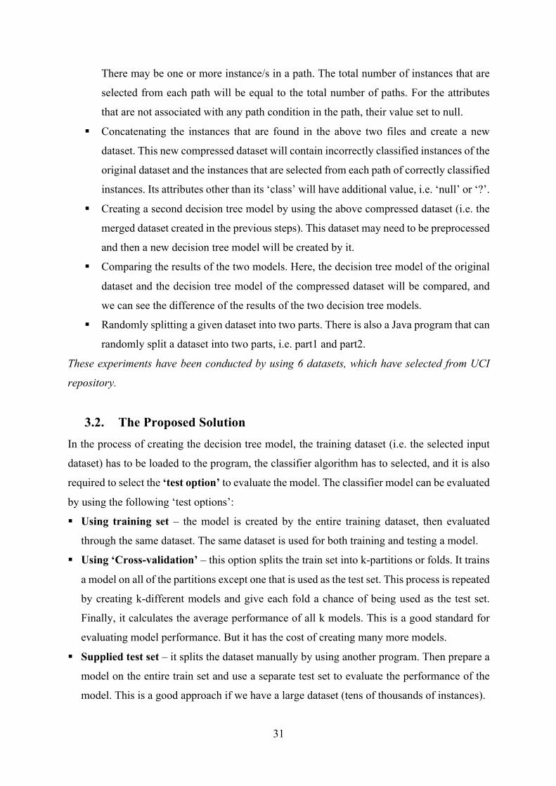
3.2. The Proposed Solution In the process of creating the decision tree model, the training dataset (i.e. the selected input
dataset) has to be loaded to the program, the classifier algorithm has to selected, and it is also
required to select the ‘test option’ to evaluate the model. The classifier model can be evaluated
by using the following ‘test options’:
§ Using training set – the model is created by the entire training dataset, then evaluated
through the same dataset. The same dataset is used for both training and testing a model.
§ Using ‘Cross-validation’ – this option splits the train set into k-partitions or folds. It trains
a model on all of the partitions except one that is used as the test set. This process is repeated
by creating k-different models and give each fold a chance of being used as the test set.
Finally, it calculates the average performance of all k models. This is a good standard for
evaluating model performance. But it has the cost of creating many more models.
§ Supplied test set – it splits the dataset manually by using another program. Then prepare a
model on the entire train set and use a separate test set to evaluate the performance of the
model. This is a good approach if we have a large dataset (tens of thousands of instances).

32
§ Percentage split – randomly split the dataset into training and testing partitions each time
when we evaluate a model. This can give us a very quick estimate of performance. Like
using a supplied test set, this one is also preferable only when we have a large dataset.
The first two ‘test options’, ‘using full training set’ and ‘10-folds cross-validation’, have used
throughout the experiments.
Fig.10. classifier, test options, and classifier output in WEKA Explorer
After selecting the test option and run the program, we see different evaluation results for each
selected test option in the ‘classifier output’ section. The ‘classifier output’ shows the
following information about the evaluation of the model.
§ Header information – it contains information about the name of the relation, the number
of instances in the training dataset, the number of attributes of the training dataset, the
attributes of the dataset including the class attribute, and the selected test mode.
§ The classifier model – it is the J48 pruned tree built-in by using the full train set. The tree
has root, internal, and leaf nodes. The number of leaves in the tree, the size of the tree, and
the time taken to build the model have displayed next to the tree. The leaves indicate the
paths of the tree, the number of leaves of the tree equal to the number of paths of the tree.
The number of leaves in the tree, the size of the tree, and the time taken to build the classifier
model have computed during the process of building the tree.
§ The evaluation of the model – it provides information about the general summary statistics,
the accuracy of the model by class, and the confusion matrix of the model. If the selected

33
‘test option’ is ‘Using training set’, the ‘time taken to test the model on training data’ has
been computed and displayed first. The evaluation results are different for each selected test
option.
The summary statistics includes information about the number of correctly and incorrectly
classified instances with their respective percentages, kappa statistic, mean absolute error, root
mean squared error, relative absolute error, root relative squared error, and the total number of
instances used for the train set.
§ Correctly and incorrectly classified instances – are the instances that are correctly or
incorrectly classified by the classifier model. The sum of the two groups of instances gives
the total number of instances available in the full training dataset. The percentage of
correctly and incorrectly classified instances have computed and displayed as well. Their
values are varied for each test option.
§ Kappa statistic – it is a chance-corrected measure of compliance between the true classes
and the classifications. Its value is calculated by taking the agreement expected by chance
and dividing by the maximum possible agreement. If the value is greater than 0, it refers
that the classifier is doing better than chance.
§ Mean absolute error – measures the average magnitude of the errors in a set of forecasts,
without considering their direction.
§ Root mean squared error – is a quadratic scoring rule which measures the average
magnitude of the error.
§ Relative Absolute Error – measures the performance of a predictive model. Relative
absolute error is not the same with relative error. Relative error is a general measure of
precision or accuracy.
§ Root Relative Squared Error – The relative squared error takes the total squared error and
normalizes it through dividing by the total squared error of the simple predictor.
§ Total number of instances – shows the size of the training dataset.
The detailed accuracy by class provides information about True Positive (TP) Rate, False
Positive (FP) Rate, Precision, Recall, F-Measure, MCC, ROC Area, and PRC Area, all by class.
It also shows the weighted average of all these metrics.
§ TP (True Positives) Rate – rate of instances that are correctly classified as a given class
§ FP (False Positives) Rate – rate of instances that are incorrectly classified as a given class
§ Precision – refers the proportion of instances that are truly classified as a given class divided
by the total number of instances classified as that class.

34
§ Recall – it is equivalent to TP rate, which refers the proportion of instances classified as a
given class divided by the actual total number of instances in that class.
§ F-Measure – it is a combined measure of precision and recall, which is calculated as (2 *
Precision * Recall / (Precision + Recall)). F-measure is a different type of accuracy measure
that takes into account class imbalances, precision and recall.
§ Matthews Correlation Coefficient (MCC) – it is an reliable statistical rate. If the
prediction obtained good results in all of the four confusion matrix categories (true positives,
false positives, true negatives, and false negatives), MCC produces a high score
proportionally both to the size of positive and negative elements in the dataset.
§ An ROC (Receiver Operating Characteristic) Curve – is a graph that shows the
performance of a classification model at all classification thresholds. This curve plots two
parameters such as – True Positive Rate and False Positive Rate.
§ PRC (Precision Recall Curve) – is an alternative to a ROC curve.
The last section, in the classifier output window, is the confusion matrix. A confusion matrix
summarizes the prediction results of a J48 classification model. The total number of correct
and incorrect predictions are summarized and map into each class. This is the key to the
confusion matrix. The confusion matrix shows how the classification model is confused when
it performs predictions of each class.
The confusion matrix gives an insight not only about the errors being made by the classifier but
more importantly about the types of errors that are being made. The process of calculating a
confusion matrix includes the following steps:
a. Acquiring a test or validation dataset with expected outcome values.
b. Making a prediction for each row in the test dataset.
c. For each class, count the number of correct and incorrect predictions from the expected
outcomes and predictions.
Then, these values are organized into a table or a matrix. Each row of the matrix corresponds
to a predicted class while each column of the matrix corresponds to an actual class. The values
of number of correct and incorrect classification are filled in a matrix.

35
The total number of correct predictions for a class go into the expected row for that class value
and the predicted column for that class value. Similarly, the total number of incorrect
predictions for a class go into the expected row for that class value and the predicted column
for that class value.
In the following sections, we will see about preparing the dataset, preprocessing it, and
conducting the experiments by using the preprocessed dataset. The dataset needs to be prepared
and pre-processed before using it for the experiments. Then the dataset will be ready for
processing both by the Java programs and by WEKA Explorer. However, in WEKA Explorer,
when we tried to load a dataset that has large number of instances (in this case, >=16138), the
program shuts automatically, and the following ‘OutOfMemory’ message have pop-up. The
WEKA Explorer that has installed and used is – ‘weka-3-8-4-azul-zulu’.
3.3. Preparing the Dataset The datasets used for this experiment have downloaded from the UC Irvine Machine
Learning Repository, in short - UCI repository (https://archive.ics.uci.edu/ml/datasets.php).
The UCI Machine Learning Repository provides databases, domain theories, and data
generators, which are used by machine learning community for the empirical analysis of
machine learning algorithms. This repository provides 557 datasets as a service to the machine
learning community. It has been widely used by students, educators, and researchers all over
the world as a primary source of machine learning datasets. The datasets can be seen through
a searchable web interface.
The first dataset used here is ‘carEvaluation’ dataset. It is compressed from simple hierarchical
decision tree model that is useful for testing constructive induction and structure discovery
methods. This dataset has the following characteristics:
§ Title: Car Evaluation Database
§ Data Set Characteristics: Multivariate

36
§ Number of Instances: 1728 (instances completely cover the attribute space)
§ Attribute Characteristics: Categorical
§ Number of Attributes: 6
§ Associated Tasks: classification
§ Missing Attribute Values: None
Dataset Information
CAR car acceptability
. PRICE overall price
. . buying buying price
. . maint price of the maintenance
. TECH technical characteristics
. . COMFORT comfort
. . . doors number of doors
. . . persons the capacity to carry in terms of persons
. . . lug_boot it is the size of luggage boot
. . safety the estimated safety of the car
The input attributes names are found in lowercase. In addition to the target concept (CAR), the
model includes three intermediate concepts such as PRICE, TECH, COMFORT.
Car evaluation database contains structural information, which includes six input attributes.
These are – buying, lug_boot, maint, persons, doors, and safety. The database is important to
test constructive induction and structure discovery methods.
Attribute Information
Class Values Are: unacc, acc, good, vgood
ð unacc – unacceptable and acc – acceptable
Attributes and their values:
buying: vhigh, high, med, low
maint: vhigh, high, med, low
doors: 2, 3, 4, 5more
persons: 2, 4, more
lug_boot: small, med, big

37
safety: low, med, high
Class Distribution (number of instances per class)
class N N[%]
unacc 1210 (70.023 %)
acc 384 (22.222 %)
good 69 ( 3.993 %)
v-good 65 ( 3.762 %)
3.4. Preprocessing the Dataset
The next task is preprocessing the ‘carEvaluation’ dataset by using WEKA Explorer and make
the dataset ready for processing. WEKA (Waikato Environment for Knowledge Analysis)
Explorer has already downloaded and installed to the PC.
Data preprocessing is the task of cleaning the dataset, instance selection, normalization,
transformation, feature extraction and selection, etc. The final result of data preprocessing is
the final training dataset. Data pre-processing may affect the way in which outcomes of the
final data processing can be interpreted.
First, the downloaded dataset (i.e. car.data) is converted to attribute-relation file format – arff
(i.e. car.arff). The header information that includes @RELATION, @ATTRIBUTE and
@DATA declarations have added to the dataset. There are two sections in Attribute-Relation
File Format (ARFF) file. These are – the header and data sections. In the header part, the line
that begins with a ‘%’ symbol is a comment. All declarations in the header including
@RELATION, @ATTRIBUTE and @DATA are case insensitive. @DATA indicates the
beginning of the data or instances. The preprocessing task can be done by WEKA Explorer
interface.
Creating a decision tree model can also be done by using WEKA Explorer interface. As it has
shown in the following figure, in the ‘Preprocess’ section of the WEKA Explorer window,
there is a button to open the prepared dataset and load to the Explorer Window. If the dataset
to be loaded doesn’t prepared well, it can’t be loaded to the program. If it is opened and loaded,
we can get information about the dataset such as – relation name, number of instances of the
dataset, and the number of attributes of the dataset. The attributes of the dataset have listed on

38
the left part of the window. On the right part, we can get the possible values of each attribute
together with their count and weight. An attribute has distinct values.
Fig.11. car.arff dataset in WEKA Explorer
The bar on the right bottom side shows, the number of instances by class for the selected
attribute. To classify the dataset in WEKA Explorer, click on the ‘Classify’ tab, then ‘choose’
the ‘Classifier’, then select the ‘Test Option’, and finally ‘start’ the classification. The
‘Classifier Output’ will be displayed on the right side.
1. Create a decision tree model based on WEKA on the entire dataset?
The decision tree model can be created by using WEKA Explorer interface as it has indicated
in fig. 11. On the other hand, the decision tree model can be created by using a Java program,
which is the main aim of the thesis. Therefore, it is possible to create the classifier model and
the evaluation of the model in both cases. This section will discuss more in brief about how to
create the classifier model, evaluate it and extract information from the model through a Java
program that uses WEKA libraries. At first, Eclipse IDE, has to be installed to develop and run Java programs. In order to develop
Java programs based on WEKA, it is required to ‘Configure Build Path’ of the ‘package’ and
add the required jar file (i.e. ‘weka.jar’). This enables to import WEKA libraries, which are
required to create the decision tree model by the selected dataset and extract information from

39
the classifier model. WEKA libraries have written in Java and they are open source, which
provide a set of APIs that allow to write code to generate decision tree models and to extract
information from the tree.
In order to create and built the classifier model as well as to evaluate the built-in model, the
following tasks have been done in the program.
§ Loading the pre-processed training dataset to the program. Here, it is required to write the
file path of the input dataset. It is the dataset on which the classifier model will be built. This
dataset may be small, medium, or large in size and has a number of attributes including the
‘class’ attribute.
§ Telling the program about which attribute of the training dataset is the class index. The class
index indicates the target attribute that is used for classification. By default, in an ARFF file,
the class index is the last attribute. “numAttributes () – 1” indicates that the class is the last
attribute. But sometimes the class attribute may be an attribute that is different from the last
attribute. The following line of code is used to set the class index of the training dataset to
the last attribute.
trainDataset.setClassIndex(trainDataset.numAttributes() - 1);
§ Creating and building the classifier model. The decision tree classifier that is used here is,
the J48 classifier, it creates and builds the classifier model of the loaded training dataset.
The following lines of code are used to initialize and build the classifier model.
J48 tree = new J48();
tree.buildClassifier(trainDataset);
§ Loading the test dataset to evaluate the built-in classifier model. The test dataset is used to
evaluate the classifier model that has created and built by the training dataset. A copy of the
training dataset has used as the test dataset. Hence, the test set has the same number of
instances and attributes like the training dataset.
§ Setting the class index of the test dataset to the last attribute. Like, in training dataset, the
class attribute of the test dataset is the last attribute, since the datasets are the same. Hence,
the following line of code sets the class index of the test dataset to the last attribute.
testDataset.setClassIndex(trainDataset.numAttributes() - 1);

40
§ Evaluating the classifier model. After building the classifier model, it is required to evaluate
the built-in model. The evaluation has initialized with the training dataset and evaluated by
using the test dataset. The following lines of code will do the evaluation.
Evaluation eval = new Evaluation(trainDataset); Random rand = new Random (1); int folds = 10;
There are two options to evaluate the model. The first one, is by using the full train set.
eval.evaluateModel(tree, testDataset); //using the full training set
The other is by using 10-folds cross-validation as in the following way.
eval.crossValidateModel(tree, testDataset, folds, rand); //using cross-validation
The following lines of code are used to get information about the training dataset.
System.out.println("Relation: " + trainDataset.relationName() + "\n");
System.out.println("Instances: " + trainDataset.numInstances() + "\n");
System.out.println("Attributes: " + trainDataset.numAttributes() + "\n");
The following loop is used to print the attributes of the training dataset, given the number of
attributes.
for(int i=0; i<7; i++) { System.out.println(trainDataset.attribute(i).name() + "\n"); } The following line of code prints the J48 pruned tree, the number of leaves and the size of the
tree, in string format.
System.out.println(tree.toString()+"\n");
The evaluation results can be printed by the following lines of code.
System.out.println(eval.toSummaryString("=== Summary ===\n", false)); System.out.println(eval.toClassDetailsString("=== Detailed Accuracy By Class ===\n")); System.out.println(eval.toMatrixString("=== Confusion Matrix ===\n"));
The sample of the built-in classifier model looks the following.

41
Number of Leaves: 131
Size of the tree: 182
Time taken to build model: 0.01 seconds
As it has shown on the above tree, ‘safety’ is the root attribute. The ‘J48 pruned tree’ has 131
number of leaves, the size of the tree is 182, and the time taken to build the model is 0.01
seconds. In the classifier output screen, for a small dataset classification, "time taken for model
build" is usually 0 seconds because the best resolution WEKA gives (default) is 0.01 seconds.
After evaluating the classifier model, we can get the following summary information.
System.out.println(eval.toSummaryString(“=== Summary ===\n”, false));
=== Summary ===
Correctly Classified Instances 1598 92.4769%
Incorrectly Classified Instances 130 7.5231%
Kappa statistic 0.8376
Mean absolute error 0.0421
Root mean squared error 0.1718
Relative absolute error 18.3833%
Root relative squared error 50.8176%
Total Number of Instances 1728

42
As a result, 1598 (92.5%) of the instances are correctly classified by the model while 130
(7.5%) of the instances are incorrectly classified. The result of kappa statistic is greater than 0,
which refers the classifier is doing better than chance.
The overall classification accuracy measure is given by the percentage of correctly classified
instances. The result of the detailed accuracy by class is the following:
System.out.println(eval.toClassDetailsString("=== Detailed Accuracy by Class ===\n"));
=== Detailed Accuracy by Class === TP Rate FP Rate Precision Recall F-Measure MCC ROC Area PRC Area Class
0.880 0.049 0.837 0.880 0.858 0.816 0.962 0.859 acc
0.609 0.011 0.689 0.609 0.646 0.634 0.918 0.593 good
0.960 0.054 0.976 0.960 0.968 0.895 0.983 0.992 unacc
0.877 0.010 0.770 0.877 0.820 0.814 0.995 0.808 vgood
Weighted Avg. 0.925 0.050 0.926 0.925 0.925 0.864 0.976 0.940
The result shows, true positive rate is high while the false positive rate is low.
The confusion matrix has also shown in the following:
System.out.println(eval.toMatrixString("=== Confusion Matrix ===\n");
=== Confusion Matrix ===
a b c d <-- classified as
338 11 28 7 | a = acc
17 42 0 10 | b = good
46 3 1161 0 | c = unacc
3 5 0 57 | d = vgood
If the real class is ‘acc’, there are 338 correct and 46 incorrect predictions while if the real class
is ‘good’, there are 42 correct and 27 incorrect predictions. If the real class is ‘unacc’, there are
1161 correct and 49 incorrect predictions while if the real class is ‘vgood’, there are 57 correct
and 8 incorrect predictions.

43
1. Apply the model on the entire dataset and write a code based on WEKA that
returns/stores in an output file, the set of records that are wrongly classified
by the decision tree model
Now, we are going to see about how to extract correctly and incorrectly classified instances of
the dataset and save incorrectly classified instances into a file. In order to accomplish this
target, the following tasks will be done in the program.
§ Loading the pre-processed training dataset to the program.
§ Setting the class index of the training dataset to its class attribute.
§ Creating and building the classifier model by using the J48 classifier and the training dataset.
§ Loading the test dataset to evaluate the built-in classifier model.
§ Setting the class index of the test dataset to its class attribute.
§ Evaluating the classifier model by using either of the two test options discussed previously.
§ Creating a file to store the extracted incorrectly classified instances of a dataset.
In addition, the following lines of code can do identifying incorrectly classified instances from
the dataset and write them to an output file. An array of double type that will contain prediction
values has declared and initialized by the evaluation value of the dataset.
double [] predictions = eval.evaluateModel(tree, testDataset); // using the train set
The program loops through the instances of testDataset and makes predictions.
for (int i=0; i < testDataset.numInstances(); i++) {
double realValue = testDataset.instance(i).classValue(); //real class of an instance
The wrongly classified instances are identified in the following way.
if(realValue != predictions[i]) {
bw.write(testDataset.instance(i).toString()); //instance written to a file
bw.newLine();
}
}
bw.close();
As it has shown above, the program loops through all instances of ‘testDataset’ and makes
prediction of the class of each instance. The real class value of each instance of the ‘testDataset’
is saved to a variable of double type in the following way.

44
double realValue = testDataset.instance(i).classValue();
If the value of this variable (i.e. the real class value of an instance) is equal to the predicted
class value of an instance, then an instance is correctly classified instance.
If(realValue == predictions[i])
Instace(i) is correctly classified instance;
Then the program can stores/writes this correctly classified instance to an output file. This
process will continue to check all instances of the testDataset.
If the value of a variable (i.e. the real class value of an instance) is not equal to the predicted
class value of an instance, then an instance is incorrectly classified instance.
If(realValue != predictions[i])
Instace(i) is incorrectly classified instance;
The program stores/writes this incorrectly classified instances to an output file. The loop will
continue to check all instances of the testDataset.
For this experiment, the incorrectly classified instances have selected and saved to a file. In
‘carEvaluation’ dataset, if the selected test mode is ‘using training set’, the number of
incorrectly classified instances are 64. But when ‘10-folds cross-validation’ has selected as test
mode, the number of incorrectly classified instances are 130. Therefore, the number of
incorrectly classified instances are not equal for each selected test mode.
The program iterates to store all incorrectly classified instances from test dataset into an output
file. In the output file, it is possible to add @RELATION, @ATTRIBUTE, and @DATA
declarations on the header section. This enables the newly created dataset that contains
incorrectly classified instances, to be recognized as an ‘arff’ file and can be loaded to WEKA
Explorer or used for processing by Java programs. A dataset file that doesn’t include those
declarations on the header section, can’t be recognized as an ‘arff’ file in WEKA Explorer. The
values of these declarations will be the same as to the declaration values in the original dataset
file. Because these incorrectly classified instances are some part of the original dataset and
have the same attributes as of it. Therefore, the header information will be the same.

45
2. Apply the model on the entire dataset and write a code based on WEKA that
returns/stores in an output file the paths of the decision tree that correctly
classify at least one of the input data. For each of those paths count also how
many records are correctly classified by it. In the program that can do this task, we are going to do the following things:
§ Loading the pre-processed training dataset to the program.
§ Telling the program about which attribute of the training dataset is the class index.
§ Creating and building the classifier model by using the J48 classifier and the training dataset.
Then, it is required to generate the source strings of the J48 pruned tree, print it to the output
screen, copy and save the source strings by the class name given in parenthesis. This class
is used to return the paths of correctly and incorrectly classified instances. The following
line of code is used to print the source strings of the built-in tree into an output screen.
System.out.println(tree.toSource(“TreeSource”));
The tree source strings of the J48 pruned tree can be get by toSource() method of the J48
class. The toSource() method is of String type and returns tree as an if-then statement. Then
this tree source with an if-then statement is saved to another Java class (i.e.
‘TreeSource.java’) and modified to return the path of each instance. In this Java class, there
is a public variable that can be accessible from other class, which is used to map each
attribute with its value. Each attribute of an instance is associated with its value.
§ Loading the test dataset to evaluate the built-in classifier model.
§ Setting the class index of the test dataset to the class attribute.
§ Evaluating the classifier model by using either of the two test options.
The following code is used to find paths of correctly classified instances by using the tree
source strings. In addition, the program enables to count the number of instances that are found
in each path. An array of double type that will contain prediction values has initialized first by
the evaluation value of the dataset.
double[] predictions = eval.evaluateModel(tree, testDataset);
The instance path is of String type and it has first initialized to null.
String instancePath = null;

46
There is another variable to save a map of each path string with the number of instances that
are available on that path. In the map, the key is the path string while the value is the number
of instances on that path.
Map<String, Integer> numRecordes = new HashMap<String, Integer> ();
The program loops through the instances of ‘testDataset’ and makes prediction of a class for
each instance. Inside the loop, the real class value of each instance of the ‘testDataset’ has
saved to a variable of double type. The tree source class is used to get the path strings for any
given instance.
for (int i=0; i < testDataset.numInstances(); i++) {
TreeSource.classify(testDataset.instance(i).toString().split(","));
double realValue = testDataset.instance(i).classValue(); // test data
The paths of correctly classified instances have saved in the following way.
if(realValue == predictions[i]) {
int count = 0;
instancePath = TreeSource.anAttributeWithItsValue.toString();
The number of instances in a path have been counted in this way.
if(numRecordes.get(instancePath) != null) {
count = numRecordes.get(instancePath);
}
count++;
numRecordes.put(instancePath, count);
}
}
For each instance, if the real class value of an instance is equal with the predicted value, the
instance is correctly classified instance. Then an instance is added to the path. In the path, each
attribute of an instance is assigned with its value (including null value) and separated by
comma. Finally, the path will display in curly braces.
A file has created by File(), FileOutputStream(), and BufferedWriter() functions to store the
output. Then each map of a path with count of instances in that path have written into the
created file. The program iterates to write all paths with respective counts into an output file.
There are 1598 correctly classified instances. These instances are found in 131 number of paths.
The sample result will be the following:

47
The number of paths are: 131
As it has indicated above, the number at the beginning of each line indicate the number of
instances available on that path and followed by the path string indicated in curly braces.
In the previous sections, the Java programs have been developed to create and built decision
tree model, extract correctly and incorrectly classified instances, extract paths of correctly and
incorrectly classified instances. Therefore, we have the set of records that are correctly
classified and the associated paths (a record in the path of the tree that is used to correctly
predict the class label for that record) and the set of records that are wrongly classified.
3. Store one record for each of the paths that are used to predict the class label
for the correct predictions in a second file. For this program, it is also required to follow the steps, which have been done for the previous
tasks. These are:
§ Loading the pre-processed training dataset to the program.
§ Setting the class index of the training dataset to its class attribute.
§ Creating and building the classifier model by using the J48 classifier and the training dataset.
Then it is required to generate the source strings of the J48 pruned tree, print it to the output
screen, copy and save the source strings by the class name given in parenthesis. This class

48
is used to return the paths of correctly and incorrectly classified instances. The following
line of code is used to print the source strings of the built-in tree into the output screen.
System.out.println(tree.toSource(“TreeSource”));
The tree source strings that are in an if-then statement are saved to another Java class (i.e.
‘TreeSource.java’) and modified to return the path of each instance. In this Java class, there
is a public variable that can be accessible from other class, which is used to map each
attribute with its value. Each attribute of an instance is associated with its value.
§ Loading the test dataset to evaluate the built-in classifier model.
§ Setting the class index of the test dataset to the class attribute.
§ Evaluating the classifier model by using either of the two test options.
§ Creating a file to store the instances extracted from each path. File(), FileOutputStream(),
and BufferedWriter() functions have been used to create a new file.
The following lines of code are used to add correctly classified instances into paths.
double [] predictions = eval.evaluateModel(tree, testDataset);
Set<String> paths = new HashSet<String>();
for (int i=0; i < testDataset.numInstances(); i++) {
The following line of code is used to split the attributes of an instance through comma.
TreeSource.classify(testDataset.instance(i).toString().split(","))
double realValue = testDataset.instance(i).classValue(); // test data
The following code is used to add a path of correctly classified instances into 'paths'
if(realValue == predictions[i]) paths.add(TreeSource.anAttributeWithItsValue.toString());
}
The following lines of code are used to extract a single instance from a path, and this will be
done for all paths of correctly classified instances.
For each path in paths:
for(String path : paths){ String attrWithValue = path.replace("}", "");
String [] attr = new String[7]; // the instances have 7 attributes

49
For each string is a path: for(String str:attrWithValue.split(",")) { if(str.contains("buying")) attr[0] = str.substring(str.lastIndexOf("=")+1); if(str.contains("maint")) attr[1] = str.substring(str.lastIndexOf("=")+1); if(str.contains("doors")) attr[2] = str.substring(str.lastIndexOf("=")+1); if(str.contains("persons")) attr[3] = str.substring(str.lastIndexOf("=")+1); if(str.contains("lug_boot")) attr[4] = str.substring(str.lastIndexOf("=")+1); if(str.contains("safety")) attr[5] = str.substring(str.lastIndexOf("=")+1); attr[6] = str.substring(str.lastIndexOf("=")+1); } attr[1] = "," + attr[1]; attr[2] = "," + attr[2]; attr[3] = "," + attr[3]; attr[4] = "," + attr[4]; attr[5] = "," + attr[5]; attr[6] = "," + attr[6]; bw.write(attr[0] + attr[1] + attr[2] + attr[3] + attr[4] + attr[5] + attr[6]); bw.newLine();
This program stores, one record for each of the paths that are used to predict the class label for
the correct predictions, into an output file. The attributes are categorical attributes. Categorical
attributes represent discrete values, which belongs to a specific finite set of categories or
classes. These are also known as classes or labels in the context of attributes or variables which
are to be predicted by a model (popularly known as response variables). Hence, each path
contains a set of ‘attribute=value’ conditions for the instances. One instance from each path
has been stored into an output file. For the attributes that are not associated with any path
condition in the path, their value has set to null. For instance, suppose that the input records are
characterised by 6 attributes (buying, maint, doors, persons, lug_boot, safety) and consider the
path buying=’high’, doors=’3’, lug_boot=’small’, and safety=’med’. In this case, the program
inserts the following record into an output file:
buying=’high’, maint=’null’, doors=’3’, persons= ‘4’, lug_boot=’small’, and safety=’med’
Here, null refers the null value, not the ‘null’ string.

50
Therefore, the program puts null for the attribute/s that is/are not associated with any path
condition.
4. Concatenate the two files created above into one compressed file? Now, we are going to concatenate the two files created before. These are: a file that contains
incorrectly classified instances and a file that contains one record for each path of correctly
classified instances. A program has been developed to concatenate/merge these two files into
one another output file (i.e. ‘mergedFile.arff’).
In the program, PrintWriter() object has been created and initialized to write records into
‘mergedFile.arff’. This object, as a parameter, receives the file path to put the merged file. Then
BufferedReader() object has been created and initialized to hold incorrectly classified
instances. This object also, as a parameter, receives the path of the input file to be written to
the merged file. Then the program loops to write each line of incorrectly classified instances to
‘mergedFile.arff’ file. The second BufferedReader() object has been created and initialized to
hold the records of the second input file. It receives as a parameter, the path of the second input
file that contains instances to be added with the previously added instances of the merged file.
Then the program iterates to write each line of this file to ‘mergedFile.arff’ file. Finally, it is
required to close all resources.
As a result, the first input file (i.e. a file that contains incorrectly classified instances) has 64
instances and the second input file (i.e. a file that contains single record of each path) has 131
instances. Then a merged file has 195 instances. The attributes other than the class attribute in
the second input file have additional attribute value (i.e. they can be null). As a result, in the
merged file, the attributes other than the class attribute will have null value as well.
5. Train a classification model on the merged file created above and check the
quality of the trained model by using a cross validation approach. The merged file (‘mergedFile.arff’) has 195 instances and 7 attributes including the ‘class’
attribute. However, unlike the original dataset (i.e. ‘car.arff’) attributes, each attribute of the
merged file have additional value (i.e. null value). For example, ‘buying’ attribute has values
such as: high, low, med, vhigh, and null.
Previously, we have seen about the program that has been developed to create a decision tree
model for the ORIGINAL dataset (i.e. ‘car.arff’). Now, we can use the same program to create
a decision tree model for the NEW compressed dataset (i.e. ‘mergedFile.arff’). This new

51
dataset may need to be preprocessed at first and then build a model. After creating a decision
tree model for the NEW compressed dataset (i.e. ‘mergedFile.arff’), we can compare the results
of the two models and the comparison results have been saved into the other file.
The new compressed dataset (i.e. ‘mergedFile.arff’) has classified by using the J48 Classifier
and by selecting ’10-folds cross-validation’ as the test mode. The following is the sample of
the built-in classifier model.
Number of Leaves: 38
Size of the tree: 49
Time taken to build model: 0.03 seconds
As it has shown above, the root attribute of this new tree is ‘doors’. The tree has 38 number of
leaves, the size of the tree is 49, and the time taken to build the tree is 0.03 seconds.
The evaluation summary statistics looks the following:
=== Summary ===
Correctly Classified Instances 138 70.7692 %
Incorrectly Classified Instances 57 29.2308 %
Kappa statistic 0.5746
Mean absolute error 0.1769
Root mean squared error 0.3291
Relative absolute error 50.4488 %
Root relative squared error 78.6485 %
Total Number of Instances 195

52
As a result, 70.8% of the instances are correctly classified while 29.2% of the instances are
incorrectly classified. Then the accuracy of the compressed dataset model is less than the
accuracy of the original dataset model.
The evaluation result provides also the following detailed accuracy by class. === Detailed Accuracy By Class ===
TP Rate FP Rate Precision Recall F-Measure MCC ROC Area PRC Area Class
0.819 0.236 0.670 0.819 0.737 0.566 0.824 0.735 acc
0.379 0.108 0.379 0.379 0.379 0.271 0.821 0.349 good
0.855 0.032 0.937 0.855 0.894 0.842 0.924 0.882 unacc
0.360 0.035 0.600 0.360 0.450 0.407 0.879 0.597 vgood
Weighted Avg. 0.708 0.119 0.712 0.708 0.703 0.599 0.866 0.712
The confusion matrix of the model looks the following.
=== Confusion Matrix ===
a b c d <-- classified as
59 7 3 3 | a = acc
14 11 1 3 | b = good
8 2 59 0 | c = unacc
7 9 0 9 | d = vgood
When the real class is ‘acc’, 59 correct and 13 incorrect predictions. When the real class is
‘good’, 11 correct and 18 incorrect predictions. For ‘unacc’ – 59 correct and 10 incorrect
predictions, for ‘vgood’ – 9 correct and 16 incorrect predictions.
6. Compare the achieved results of the decision tree model of the original
dataset and the compressed (merged) dataset? Previously, two decision tree models have been created and built by the 1st original dataset (i.e.
‘car.arff’) and the compressed new dataset (i.e. ‘mergedFile.arff’) respectively. The two
datasets have different number of instances but the same number of attributes. Unlike the
attributes of the original dataset, the attributes other than the class attribute of the new
compressed dataset have an additional value, i.e. ‘null’ or ‘?’. The new dataset may need pre-
processing before creating the model through it. Since the number of instances in the two
datasets are different, the classifier model of the two datasets are different. They have different
J48 Pruned Tree, different number of leaves, and different size of the tree. In addition, the
evaluation results of the two data sets’ classifier models are different. They have different
summary statistics, detailed accuracy by class, and confusion matrix results.

53
7. Randomly split the instances in the original dataset in two parts and write
them into two files Another program has been developed, which randomly splits any given dataset in two parts
and write the split instances into two different files.
The following tasks have been done in the program.
§ Loading the pre-processed training dataset to the program. This is the dataset to be split.
§ Creating a file to store the instances of Part1 and Part2. File(), FileOutputStream(), and
BufferedWriter() functions have been used to create the new files that are used to store the
contents of Part1 and Part2.
The following lines of code randomly splits instances and writes them into two output files.
for (i = 0; i < trainDataset.numInstances(); i++) { if (Math.random() < 0.5) {
bw.write(trainDataset.instance(i).toString()); // writes an instance into part1 bw.newLine();
} else {
bw2.write(trainDataset.instance(i).toString()); // writes an instance into part2 bw2.newLine();
} } bw.close(); bw2.close(); It is also possible to write @RELATION, @ATTRIBUTE, and @DATA declarations at the
header section of each file, to make files an ‘arff’ file.
As it has shown in the above program, the loop iterates up to the total number of instances of
the dataset to randomly split and write the instances into the files. The random splitting of the
instances has done by Math.random() function. Math.random() function returns a pseudo-
random floating point number between 0 (inclusive) and 1 (exclusive). With 0 included and 1
excluded (therefore in the interval [0, 1)), scalable to the desired range. The implementation
selects an initial (seed) number useful for the generation algorithm to return random numbers,
which cannot be chosen or reset by the user. For each instance, if the value of Math.random() is
less than 0.5, that instance is saved to the 1st file. If the value of Math.random() is greater than
0.5, that instance is saved to the 2nd file. The splitting and writing processes have done for all
instances of the dataset. Finally, the two files have to be closed.

54
Chapter Four
Experimental Results
In chapter three, we have discussed about the issues that the thesis has tryied to address, the
designed methodologies that have been used to address the problems, and the proposed
solutions. In this chapter, we will discuss about the experimental results of the methodologies
designed before, by using five datasets that are selected from UCI repository. The selected
datasets are adult.data, balance-scale.data, iris.data, PhishingData.arff, and tae.data.
These datasets have been converted to ARFF format and pre-processed in WEKA Explorer.
Before discussing about the experimental results, first let us discuss about the selected datasets.
The information about each dataset is described as follows.
1. Adult Dataset (adult.arff)
Dataset Characteristics: Multivariate Number of instances: 32561
Attribute Characteristics: Categorical, Integer Number of attributes: 14 + class attribute
Associated Tasks: Classification Missing Values: Yes
Attributes and their values
age: continuous
workclass: Private, Self-emp-not-inc, Self-emp-inc, Federal-gov, Local-gov, State-gov,
Without-pay, Never-worked
fnlwgt: continuous
education: Bachelors, Some-college, 11th, HS-grad, Prof-school, Assoc-acdm, Assoc-voc,
9th, 7th-8th, 12th, Masters, 1st-4th, 10th, Doctorate, 5th-6th, Preschool
education-num: continuous
marital-status: Married-civ-spouse, Divorced, Never-married, Separated, Widowed, Married-
spouse-absent, Married-AF-spouse
occupation: Tech-support, Craft-repair, Other-service, Sales, Exec-managerial, Prof-
specialty, Handlers-cleaners, Machine-op-inspct, Adm-clerical, Farming-fishing,
Transport-moving, Priv-house-serv, Protective-serv, Armed-Forces
relationship: Wife, Own-child, Husband, Not-in-family, Other-relative, Unmarried

55
race: White, Asian-Pac-Islander, Amer-Indian-Eskimo, Other, Black
sex: Female, Male
capital-gain: continuous
capital-loss: continuous
hours-per-week: continuous
native-country: United-States, Cambodia, England, Puerto-Rico, Canada, Germany,
Outlying-US(Guam-USVI-etc), India, Japan, Greece, South, China, Cuba, Iran, Honduras,
Philippines, Italy, Poland, Jamaica, Vietnam, Mexico, Portugal, Ireland, France, Dominican-
Republic, Laos, Ecuador, Taiwan, Haiti, Columbia, Hungary, Guatemala, Nicaragua, Scotland,
Thailand, Yugoslavia, El-Salvador, Trinadad&Tobago, Peru, Hong, Holand-Netherlands
class attribute values are: <=50K and >50K
2. Balance Scale Dataset (balance-scale.arff)
This dataset was generated to model psychological experimental results. Each instance is
classified as having the balance scale tip to the right, tip to the left, or be balanced. The
attributes are the left weight, the left distance, the right weight, and the right distance. The
correct way to find the class is the greater of (left-distance * left-weight) and (right-distance *
right-weight). If they are equal, it is balanced.
Dataset Characteristics: Multivariate Associated Tasks: Classification
Attribute Characteristics: Categorical Number of attributes: 4(numeric) + class attribute
Number of instances: 625 (49 balanced, 288 left, 288 right) Missing Values: No
Attribute Information:
a. Class Name: 3 (L, B, R) – it is the class attribute.
b. Left-Weight: 5 (1, 2, 3, 4, 5)
c. Left-Distance: 5 (1, 2, 3, 4, 5)
d. Right-Weight: 5 (1, 2, 3, 4, 5)
e. Right-Distance: 5 (1, 2, 3, 4, 5)
Missing Attribute Values: none

56
Class Distribution:
i. 46.08 percent are L
ii. 07.84 percent are B
iii. 46.08 percent are R
3. Iris Dataset (Iris.arff)
This is the best-known database to be found in the pattern recognition literature. The dataset
contains 3 classes of 50 instances each, where each class refers to a type of iris plant. One class
is linearly separable from the other 2; the latter are NOT linearly separable from each other.
Dataset Characteristics: Multivariate Associated Tasks: Classification
Attribute Characteristics: Real Missing Values: No
Number of instances: 150 (50 in each of three classes)
Number of Attributes: 4 numeric, predictive attributes and the class
Attribute Information:
a. sepal length in cm
b. sepal width in cm
c. petal length in cm
d. petal width in cm
e. class values: Iris Setosa, Iris Versicolour, and Iris Virginica
Missing Attribute Values: None
Summary Statistics:
Min Max Mean SD Class Correlation
sepal length: 4.3 7.9 5.84 0.83 0.7826
sepal width: 2.0 4.4 3.05 0.43 -0.4194
petal length: 1.0 6.9 3.76 1.76 0.9490 (high!)

57
petal width: 0.1 2.5 1.20 0.76 0.9565 (high!)
Class Distribution: 33.3% for each of 3 classes.
4. Website Phishing Dataset (PhishingData.arff)
Phishing websites were collected from Phishtank data archive (www.phishtank.com), which is
a free community site where users can submit, verify, track and share phishing data. When a
website is considered SUSPICIOUS that means it can be either phishy or legitimate, meaning
the website held some legit and phishy features.
Dataset Characteristics: Multivariate Number of instances: 1353
Attribute Characteristics: Integer Number of attributes: 10
Associated Tasks: Classification Missing Values: N/A
The attributes and their values:
SFH: 1, -1, 0 Web_traffic: 1, 0, -1
popUpwindow: -1, 0, 1 URL_length: 1, -1, 0
SSLfinal_State: 1, -1, 0 age_of_domain: 1, -1
Request_URL: -1, 0, 1 having_IP_Address: 0, 1
URL_of_Anchor: -1, 0, 1 Result: 0, 1, -1 (it is the class attribute)
5. Teaching Assistant Evaluation Dataset (tae.arff)
This dataset consists of evaluations of teaching performance over three regular semesters and
two summer semesters of 151 teaching assistant (TA) assignments at the Statistics Department
of the University of Wisconsin-Madison. The scores were divided into 3 roughly equal-sized
categories ("low", "medium", and "high") to form the class variable.
Dataset Characteristics: Multivariate Number of instances: 151
Attribute Characteristics: Categorical, Integer Number of attributes: 5 + class attribute
Associated Tasks: Classification Missing Values: No

58
Attribute Information:
1. Whether or not the TA is a native English speaker (binary)
1=English speaker, 2=non-English speaker
2. Course instructor (categorical, 25 categories)
3. Course (categorical, 26 categories)
4. Summer or regular semester (binary) 1=Summer, 2=Regular
5. Class size (numerical)
6. Class attribute (categorical) 1=Low, 2=Medium, 3=High
Missing Attribute Values: None
As it has discussed above, the size of adult dataset is very large, it has larger numbers of
instances than the other datasets.
In the following section, we will see the experimental results of the designed methodologies
by using the above selected datasets.
The random splitting and writing of the initial dataset into two output files.
The developed program has randomly split the instances of each dataset into two parts and
writes them into two output files as in the following way.
adult.arff
This dataset has 32561 instances. After randomly splitting and writing all of its instances,
16138 instances have been written on the first file (i.e. adult_part1.arff) and 16423 instances
have been written on the second file (i.e. adult_part2.arff).
balance-scale.arff
This dataset has 625 instances. After randomly splitting and writing all of its instances, 328
instances have been stored on the first part (i.e. balance_part1.arff) and 297 instances have been

59
stored on the second part (i.e. balance_part2.arff). The program splits and then writes each
instances of the initial dataset into two output files.
Iris.arff
This dataset has 150 instances. After the random splitting and writing process, 72 instances
have been written on the first part (i.e. iris_part1.arff) and 78 instances have been written on
the second part (i.e. iris_part2.arff).
PhishingData.arff
This dataset has 1353 instances. After randomly splitting and writing all of its instances, there
are 713 instances stored on the first part (i.e. phishing_part1.arff) and there are 640 instances
stored on the second part (i.e. phishing_part2.arff).
tae.arff
This dataset has 151 instances. After randomly splitting and writing all of its instances, 67
instances have been written on the first part (i.e. tae_part1.arff) and 84 instances have been
written on the second part (i.e. tae_part2.arff).
Decision tree model (Model#1) created by using the 1st partition of each dataset
First, it is required to include the header declarations and make part1 of each dataset as an ‘arff’
file. The selected ‘test option’ that has been used to evaluate the classifier model of each dataset
was ‘using full training set’. The decision tree model created by part1 of each dataset has the
following characteristics.
The classifier model of ‘adult_part1.arff’ dataset
This part of the dataset has 16138 number of instances. Like in the initial dataset, it has the
same and 15 attributes. In its built-in classifier model, the root attribute is ‘capital-gain’, the
tree has 371 number of leaves and the size of the tree is 480.
The evaluation result of the classifier model shows the following summary statistics, detailed
accuracy by class, and confusion matrix results.

60
=== Summary === Correctly Classified Instances 14210 88.053% Incorrectly Classified Instances 1928 11.947% Kappa statistic 0.6522 Mean absolute error 0.1803 Root mean squared error 0.2999 Relative absolute error 49.5105% Root relative squared error 70.282% Total Number of Instances 16138
As a result, 88.1% of the instances are correctly classified while 11.9% of the instances are
incorrectly classified. The kappa statistic value (i.e. 0.6522) is greater than 0, which means its
classifier is doing better than chance. The average magnitude of the errors in a set of forecasts
(i.e. mean absolute error) is 0.1803 while the average magnitude of the error (i.e. root mean
squared error) is 0.2999. The performance of a predictive model (i.e. relative absolute error) is
49.5% while root relative squared error is 70.3%. === Detailed Accuracy by Class === TP Rate FP Rate Precision Recall F-Measure MCC ROC Area PRC Area Class 0.668 0.053 0.800 0.668 0.728 0.657 0.912 0.806 >50K 0.947 0.332 0.901 0.947 0.923 0.657 0.912 0.963 <=50K Weighted Avg. 0.881 0.265 0.877 0.881 0.877 0.657 0.912 0.925 The ‘Weighted Average’ of instances correctly classified as a given class (i.e. true positive
rate) is 0.881 while instances falsely classified as a given class (i.e. false positive rate) is 0.265.
The ‘Weighted Average’ of the proportion of instances that are truly of a class divided by the
total instances classified as that class (i.e. its precision) is 0.877 while the proportion of
instances classified as a given class divided by the actual total in that class (equivalent to TP
rate), i.e. the recall, is 0.881. The ‘Weighted Average’ of the combined measure of precision
and recall (i.e. F-Measure) is 0.877. The MCC produces a high score only if the prediction
obtained good results in all of the four confusion matrix categories (TP, FP, true negatives, and
false positives), proportionally both to the size of positive elements and the size of negative
elements in the dataset. In this case, its ‘Weighted Average’ value is 0.657. The ‘Weighted
Average’ of ROC Area and PRC Area are also 0.912 and 0.925 respectively. === Confusion Matrix === a b <-- classified as 2580 1283 | a = >50K 645 11630 | b = <=50K
When the real class is ‘>50K’, there are 2580 correct and 1283 incorrect predictions. When the
real class is ‘<=50K’, there are 11630 correct and 645 incorrect predictions.

61
The classifier model of ‘balance_part1.arff’ dataset
This part of the dataset has 328 number of instances. Like in the initial dataset, it has the same
and 5 attributes. As it has shown in its built-in classifier model, the root attribute of its decision
tree is ‘rightDistance’, the number of leaves are 17 and the size of the tree is 21.
The evaluation result of the classifier model shows the following summary statistics, detailed
accuracy by class, and confusion matrix results. === Summary ===
Correctly Classified Instances 248 75.6098 % Incorrectly Classified Instances 80 24.3902% Kappa statistic 0.538 Mean absolute error 0.2428 Root mean squared error 0.3484 Relative absolute error 65.5685% Root relative squared error 81.0479% Total Number of Instances 328
Therefore, 75.6% of the instances are correctly classified while 24.4% of the instances are
incorrectly classified. The kappa statistic value (i.e. 0.538) is greater than 0, which means its
classifier is doing better than chance. The average magnitude of the errors in a set of forecasts
(i.e. mean absolute error) is 0.2428 while the average magnitude of the error (i.e. root mean
squared error) is 0.3484. The performance of a predictive model (i.e. relative absolute error) is
65.6% while root relative squared error is 81.05%. === Detailed Accuracy by Class === TP Rate FP Rate Precision Recall F-Measure MCC ROC Area PRC Area Class 0.845 0.287 0.739 0.845 0.788 0.561 0.839 0.804 L 0.000 0.000 ? 0.000 ? ? 0.737 0.136 B 0.762 0.177 0.778 0.762 0.770 0.586 0.851 0.789 R Weighted Avg. 0.756 0.220 ? 0.756 ? ? 0.838 0.756 The ‘Weighted Average’ of true positive rate is 0.756 while the ‘Weighted Average’ of false
positive rate is 0.220. The ‘Weighted Average’ of precision has not generated while the
‘Weighted Average’ of recall is 0.756 (equivalent to TP rate). The ‘Weighted Average’ of F-
Measure and MCC have also not generated. The ‘Weighted Average’ of ROC Area and PRC
Area are 0.838 and 0.756 respectively. === Confusion Matrix === a b c <-- classified as 136 0 25 | a = L 13 0 7 | b = B 35 0 112 | c = R
When the real class is ‘L’, there are 136 correct and 25 incorrect predictions. When the real
class is ‘B’, there are 20 incorrect predictions and no correct prediction. When the real class is
‘R’, there are 112 correct and 35 incorrect predictions.

62
The classifier model of ‘iris_part1.arff’ dataset
This part of the dataset has 72 number of instances. Like in the initial dataset, it has the same
and 5 attributes. As it has shown in its built-in classifier model, the root attribute of its decision
tree is ‘petalWidth’, the number of leaves are 4 and the size of the tree is 7.
The evaluation result of the classifier model shows the following summary statistics, detailed
accuracy by class, and confusion matrix results. === Summary ===
Correctly Classified Instances 70 97.2222% Incorrectly Classified Instances 2 2.7778% Kappa statistic 0.9583 Mean absolute error 0.0316 Root mean squared error 0.1256 Relative absolute error 7.1062 % Root relative squared error 26.6578 % Total Number of Instances 72
The above evaluation of the model shows that 97.2% of the instances are correctly classified
while 2.8% of the instances are incorrectly classified. The kappa statistic value (i.e. 0. 9583) is
greater than 0, which means its classifier is doing better than chance. The average magnitude
of the errors in a set of forecasts (i.e. mean absolute error) is 0.0316 while the average
magnitude of the error (i.e. root mean squared error) is 0.1256. The performance of a predictive
model (i.e. relative absolute error) is 7.1% while root relative squared error is 26.7%. === Detailed Accuracy by Class === TP Rate FP Rate Precision Recall F-Measure MCC ROC Area PRC Area Class 1.000 0.000 1.000 1.000 1.000 1.000 1.000 1.000 Iris-setosa 0.913 0.000 1.000 0.913 0.955 0.937 0.987 0.973 Iris-versicolor 1.000 0.042 0.923 1.000 0.960 0.941 0.987 0.951 Iris-virginica Weighted Avg. 0.972 0.014 0.974 0.972 0.972 0.960 0.991 0.975 The ‘Weighted Average’ of true positive rate is 0.972 while the ‘Weighted Average’ of false
positive rate is 0.014. The ‘Weighted Average’ of precision is 0.974 while the ‘Weighted
Average’ of recall is 0.972 (equivalent to TP rate). The ‘Weighted Average’ of F-Measure is
0.972 (it is also equivalent to TP rate) and the ‘Weighted Average’ of MCC is 0.960. The
‘Weighted Average’ of ROC Area and PRC Area are 0.991 and 0.975 respectively. === Confusion Matrix === a b c <-- classified as 25 0 0 | a = Iris-setosa 0 21 2 | b = Iris-versicolor 0 0 24 | c = Iris-virginica
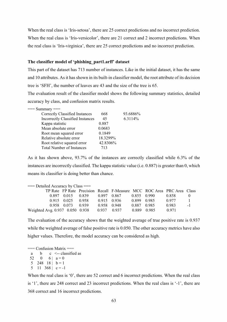
63
When the real class is ‘Iris-setosa’, there are 25 correct predictions and no incorrect prediction.
When the real class is ‘Iris-versicolor’, there are 21 correct and 2 incorrect predictions. When
the real class is ‘Iris-virginica’, there are 25 correct predictions and no incorrect prediction.
The classifier model of ‘phishing_part1.arff’ dataset
This part of the dataset has 713 number of instances. Like in the initial dataset, it has the same
and 10 attributes. As it has shown in its built-in classifier model, the root attribute of its decision
tree is ‘SFH’, the number of leaves are 43 and the size of the tree is 65.
The evaluation result of the classifier model shows the following summary statistics, detailed
accuracy by class, and confusion matrix results. === Summary ===
Correctly Classified Instances 668 93.6886% Incorrectly Classified Instances 45 6.3114% Kappa statistic 0.887 Mean absolute error 0.0683 Root mean squared error 0.1849 Relative absolute error 18.3299% Root relative squared error 42.8306% Total Number of Instances 713
As it has shown above, 93.7% of the instances are correctly classified while 6.3% of the
instances are incorrectly classified. The kappa statistic value (i.e. 0.887) is greater than 0, which
means its classifier is doing better than chance. === Detailed Accuracy by Class === TP Rate FP Rate Precision Recall F-Measure MCC ROC Area PRC Area Class 0.897 0.015 0.839 0.897 0.867 0.855 0.990 0.858 0 0.915 0.025 0.958 0.915 0.936 0.899 0.985 0.977 1 0.958 0.073 0.939 0.958 0.948 0.887 0.985 0.983 -1 Weighted Avg. 0.937 0.050 0.938 0.937 0.937 0.889 0.985 0.971 The evaluation of the accuracy shows that the weighted average of true positive rate is 0.937
while the weighted average of false positive rate is 0.050. The other accuracy metrics have also
higher values. Therefore, the model accuracy can be considered as high. === Confusion Matrix === a b c <-- classified as 52 0 6 | a = 0 5 248 18 | b = 1 5 11 368 | c = -1
When the real class is ‘0’, there are 52 correct and 6 incorrect predictions. When the real class
is ‘1’, there are 248 correct and 23 incorrect predictions. When the real class is ‘-1’, there are
368 correct and 16 incorrect predictions.

64
The classifier model of ‘tae_part1.arff’ dataset
This part of the dataset has 67 number of instances. Like in the initial dataset, it has the same
and 6 attributes. As it has shown in its built-in classifier model, the root attribute of its decision
tree is ‘summerOrSemester’, the number of leaves are 14 and the size of the tree is 27.
The evaluation result of the classifier model shows the following summary statistics, detailed
accuracy by class, and confusion matrix results. === Summary ===
Correctly Classified Instances 55 82.0896% Incorrectly Classified Instances 12 17.9104% Kappa statistic 0.7293 Mean absolute error 0.1577 Root mean squared error 0.2808 Relative absolute error 35.8721% Root relative squared error 59.9078% Total Number of Instances 67
As it has shown above, 82.1% of the instances are correctly classified while 17.9% of the
instances are incorrectly classified. The kappa statistic value (i.e. 0.7293) is greater than 0,
which means its classifier is doing better than chance. The relative absolute error and the root
relative squared error are 35.9% and 59.9% respectively. === Detailed Accuracy by Class === TP Rate FP Rate Precision Recall F-Measure MCC ROC Area PRC Area Class 0.762 0.065 0.842 0.762 0.800 0.717 0.953 0.885 1 0.895 0.104 0.773 0.895 0.829 0.759 0.965 0.892 2 0.815 0.100 0.846 0.815 0.830 0.719 0.945 0.906 3 Weighted Avg. 0.821 0.090 0.824 0.821 0.820 0.730 0.953 0.896 The evaluation of the accuracy shows that the weighted average of true positive rate is 0.821
while the weighted average of false positive rate is 0.090. The other accuracy metrics have also
higher values. Therefore, the model accuracy can be considered as high. === Confusion Matrix === a b c <-- classified as 16 2 3 | a = 1 1 17 1 | b = 2 2 3 22 | c = 3
When the real class is ‘1’, there are 16 correct and 5 incorrect predictions. When the real class
is ‘2’, there are 17 correct and 2 incorrect predictions. When the real class is ‘3’, there are 22
correct and 5 incorrect predictions.

65
The new dataset (Part1New) created from split1 of each dataset
In this section, for Part1 of each dataset, the following tasks have been done:
§ Incorrectly classified instances have been identified and saved into a file.
§ A classifier model has been built, the paths of correctly classified instances have been
extracted, and the number of instances that are available in each path are counted.
§ For all paths, a single instance from each path are selected and saved into another file.
§ Finally, the identified incorrectly classified instances have been concatenated with
instances that are selected from each path.
balance_part1.arff
1. In this part of the dataset, there are 80 incorrectly classified instances. Then they have been
identified and saved into a new file.
2. There are 248 correctly classified instances in this dataset. The following are paths of
correctly classified instances and the number of instances that are available in the path. The
path is the one inside in the curly braces. === Correctly Classified Instances === 248
13 {leftWeight=5, rightDistance=2, class=L} 12 {leftDistance=2, rightDistance=4, class=R} 10 {leftDistance=4, rightDistance=3, class=L} 5 {leftDistance=3, rightDistance=3, class=L} 14 {leftWeight=3, rightDistance=2, class=L} 9 {leftDistance=2, rightDistance=3, class=R} 8 {leftWeight=1, rightDistance=2, class=R} 58 {rightDistance=1, class=L} 11 {leftDistance=3, rightDistance=4, class=R} 6 {leftWeight=2, rightDistance=2, class=R} 10 {leftDistance=5, rightDistance=4, class=L} 11 {leftWeight=4, rightDistance=2, class=L} 13 {leftDistance=1, rightDistance=4, class=R} 9 {leftDistance=5, rightDistance=3, class=L} 9 {leftDistance=1, rightDistance=3, class=R} 44 {rightDistance=5, class=R} 6 {leftDistance=4, rightDistance=4, class=L} The number of paths are: 17
3. For each path of correctly classified instances, a single instance has been selected and stored
into another file. For this instance, in the path, if its attribute value is null, ‘null’ or ‘?’ will
be saved as a value for that attribute. As it has shown above, there are 17 paths of correctly
classified instances. Hence, 17 instances have been extracted and saved into a file.

66
4. Then, the above two datasets have been merged and written into another file (i.e.
Part1New.arff). The instances of a dataset that contains a single instance of each path of
correctly classified instances (i.e. 17 instances) and a dataset that contains incorrectly
classified instances of ‘balance_part1.arff’ (i.e. 80 instances) have been concatenated.
Therefore, this dataset will have 97 instances in total. Unlike ‘balance_part1.arff’, the
attributes other than the class attribute in this dataset has additional value (i.e. null). It is
possible to add header declarations for this new derived dataset.
iris_part1.arff
1. This dataset has 2 incorrectly classified instances and they have saved into a file. === Incorrectly Classified Instances === 2
5.9,3.2,4.8,1.8,Iris-versicolor
6,2.7,5.1,1.6,Iris-versicolor
2. The decision tree has created and there are 4 paths of correctly classified instances. The
number of instances that are available in each path are also counted and saved. === Correctly Classified Instances === 70
=== Paths of Correctly Classified Instances and count of instances in each path ===
25 {petalWidth<=0.6, class=Iris-setosa}
22 {petalLength<=5, petalWidth<=1.7, petalWidth>=0.6, class=Iris-versicolor}
3 {petalLength>5, petalWidth<=1.7, petalWidth>=0.6, class=Iris-virginica}
20 {petalWidth>1.7, class=Iris-virginica}
The number of paths are: 4
3. For each path of correctly classified instances, a single instance has selected and stored into
another file. For this instance, in the path, if its attribute value is null, ‘null’ ‘?’ can be saved
as a value for that attribute. % The number of paths of correctly classified instances are: 4
% A single instance for each path has stored as follows:
null,null,null,0.6,Iris-setosa
null,null,5,0.6,Iris-versicolor
null,null,5,0.6,Iris-virginica
null,null,null,1.7,Iris-virginica
4. Then, the instances in the above two datasets have been merged and stored into another file
(i.e. Part1New.arff). Therefore, the contents a file that contains a single instance of each
path of correctly classified instances and a file that contains incorrectly classified instances
of ‘iris_part1.arff’ are concatenated as follows:

67
% a file that contains incorrectly classified records and a file that contains % a single record for each path of correctly classified instances are merged here. @RELATION iris @ATTRIBUTE sepalLength NUMERIC @ATTRIBUTE sepalWidth NUMERIC @ATTRIBUTE petalLength NUMERIC @ATTRIBUTE petalWidth NUMERIC @ATTRIBUTE class {Iris-setosa,Iris-versicolor,Iris-virginica} @DATA 5.9,3.2,4.8,1.8,Iris-versicolor 6,2.7,5.1,1.6,Iris-versicolor null,null,null,0.6,Iris-setosa null,null,5,0.6,Iris-versicolor null,null,5,0.6,Iris-virginica null,null,null,1.7,Iris-virginica
adult_part1.arff
As it has been done in the above, the incorrectly classified instances of this part of the dataset
(i.e. 1928 instances) have been saved into a file. Its decision tree has also created and the paths
of correctly classified instances together with the count of instances that are available in each
path have been identified. The number of paths of correctly classified instances are 364. For
each path, a single instance has been extracted (364 instances in total) and stored into a file.
Finally, the contents of the files that contains incorrectly classified instances and single instance
of a path have concatenated and saved into another file (i.e. Part1New.arff). Therefore, the
number of instances in this new dataset are 2292 (i.e. 1928 + 364).
phishing_part1.arff
The dataset’s decision tree has been created and built. Its incorrectly classified instances (i.e.
45 instances) have been written into a file. The paths of correctly classified instances and the
count of instances that are available in each path have been extracted. For each path, a single
instance has been selected and written into a file. The number of paths of correctly classified
instances are 43. Then 43 instances that are extracted from all paths have been written into
another file. Finally, the instances of the two datasets have been concatenated and saved to
another file (i.e. Part1New.arff). The new derived dataset will have 88 instances.
tae_part1.arff
In this case, ‘tae_part1.arff’ has 12 incorrectly classified instances and they have been saved
into a file. Its decision tree has created and built. The paths of correctly classified instances

68
together with the count of instances that are available in each path have been extracted and
computed. The number of paths of correctly classified instances are 8. For each path, a single
instance has been selected (8 instances in total) and stored into another file. Finally, the contents
of the files that contains incorrectly classified instances and single instance of a path have
concatenated and saved into another file (i.e. Part1New.arff). This last dataset has 20 number
of instances.
The 2nd model (Model#1New) created by using ‘Part1New.arff’ of each dataset
The new decision tree models created by using the derived dataset (i.e. Part1New.arff) of the
above-mentioned datasets have discussed below.
balance_part1.arff
The decision tree model of its derived dataset (i.e. ‘Part1New.arff’) is the following:
Relation: balanceScale Instances: 97 Attributes: 5 class leftWeight leftDistance rightWeight rightDistance Test mode: evaluate on training data === Classifier model (full training set) === J48 pruned tree ------------------ rightWeight = 1: L (15.0/4.0) rightWeight = 2: L (16.0/8.0) rightWeight = 3 | leftWeight = 1: R (6.0/1.0) | leftWeight = 2: R (3.0/1.0) | leftWeight = 3: B (4.0/1.0) | leftWeight = 4: L (2.0) | leftWeight = 5: L (3.0) | leftWeight = null: R (0.0) rightWeight = 4: R (14.0/3.0) rightWeight = 5: R (17.0/4.0) rightWeight = null: L (17.0/8.0) Number of Leaves: 11 Size of the tree: 13 As it has shown above, the root attribute of the tree is ‘rightWeight’. The tree has 11 number
of leaves and the size of the tree is 13.

69
=== Summary === Correctly Classified Instances 67 69.0722% Incorrectly Classified Instances 30 30.9278% Kappa statistic 0.4989 Mean absolute error 0.2718 Root mean squared error 0.3686 Relative absolute error 63.8015% Root relative squared error 79.9278% Total Number of Instances 97
The above evaluation of the model shows that 69.1% of instances are correctly classified while
30.9% of the instances are incorrectly classified by the model. The kappa statistic value (i.e.
0.4989) is greater than 0, which means its classifier is doing better than chance. The relative
absolute error and the root relative squared error are 63.8% and 79.9% respectively. === Detailed Accuracy by Class === TP Rate FP Rate Precision Recall F-Measure MCC ROC Area PRC Area Class 0.971 0.317 0.623 0.971 0.759 0.626 0.887 0.749 L 0.150 0.013 0.750 0.150 0.250 0.279 0.743 0.400 B 0.721 0.167 0.775 0.721 0.747 0.559 0.856 0.756 R Weighted Avg. 0.691 0.188 0.716 0.691 0.649 0.525 0.843 0.680 The ‘Weighted Average’ of true positive rate is 0.691 while the ‘Weighted Average’ of false
positive rate is 0.188. === Confusion Matrix ===
a b c <-- classified as 33 0 1 | a = L 9 3 8 | b = B 11 1 31 | c = R When the real class is ‘L’, there are 33 correct predictions and 1 incorrect prediction. When the
real class is ‘B’, there are 3 correct and 17 incorrect predictions. When the real class is ‘R’,
there are 31 correct and 16 incorrect predictions.
iris_part1.arff
The decision tree model ‘Part1New.arff’of ‘iris_part1.arff’ is the following: Relation: iris Instances: 6 Attributes: 5
sepalLength sepalWidth petalLength petalWidth class Test mode: evaluate on training data

70
=== Classifier model (full training set) === J48 pruned tree ------------------ : Iris-versicolor (6.0/3.0) Number of Leaves: 1 Size of the tree: 1 === Summary ===
Correctly Classified Instances 3 50% Incorrectly Classified Instances 3 50% Kappa statistic 0 Mean absolute error 0.4074 Root mean squared error 0.4513 Relative absolute error 97.0588 % Root relative squared error 99.4987 % Total Number of Instances 6
In the above summary statistics, 50% of the instances are correctly classified and the other 50%
of the instances are incorrectly classified. The kappa statistic value is 0, which means its
classifier is doing by chance. The relative absolute error and the root relative squared error are
very high, which are 97.5% and 99.5% respectively. === Detailed Accuracy By Class === TP Rate FP Rate Precision Recall F-Measure MCC ROC Area PRC Area Class 0.000 0.000 ? 0.000 ? ? 0.500 0.167 Iris-setosa 1.000 1.000 0.500 1.000 0.667 ? 0.500 0.500 Iris-versicolor 0.000 0.000 ? 0.000 ? ? 0.500 0.333 Iris-virginica Weighted Avg. 0.500 0.500 ? 0.500 ? ? 0.500 0.389 In the above detail accuracy by class, the true and false positive rates are equal. While some of
the precision and F-Measure values are not generated. All of the MCC values are not generated. === Confusion Matrix === a b c <-- classified as 0 1 0 | a = Iris-setosa 0 3 0 | b = Iris-versicolor 0 2 0 | c = Iris-virginica When the real class is ‘Iris-setosa’, there are no correct prediction and 1 incorrect prediction.
When the real class is ‘Iris-versicolor’, there are 3 correct predictions and no incorrect
prediction. When the real class is ‘Iris-virginica’, there are no correct and 2 incorrect
predictions.
PhishingData_part1.arff
The decision tree model of its derived dataset (i.e. ‘Part1New.arff’) is the following: Scheme: weka.classifiers.trees.J48 -C 0.25 -M 2 Relation: phishing Instances: 88 Attributes: 10 SFH

71
popUpWidnow SSLfinal_State Request_URL URL_of_Anchor web_traffic URL_Length age_of_domain having_IP_Address Result Test mode: evaluate on training data === Classifier model (full training set) === J48 pruned tree ------------------ Request_URL = -1 | SSLfinal_State = 1 | | having_IP_Address = 0: -1 (10.0/2.0) | | having_IP_Address = 1: 1 (3.0) | | having_IP_Address = null | | | URL_Length = 1: 1 (2.0) | | | URL_Length = -1: -1 (3.0/1.0) | | | URL_Length = 0: 0 (2.0) | | | URL_Length = null: 0 (3.0/2.0) | SSLfinal_State = -1: 0 (8.0/2.0) | SSLfinal_State = 0 | | web_traffic = 1: 1 (0.0) | | web_traffic = 0: 1 (4.0) | | web_traffic = -1 | | | SFH = 1: -1 (2.0) | | | SFH = -1: 1 (2.0) | | | SFH = 0: 1 (0.0) | | | SFH = null: 1 (0.0) | | web_traffic = null: -1 (1.0) | SSLfinal_State = null: -1 (1.0) Request_URL = 0 | having_IP_Address = 0: -1 (4.0/1.0) | having_IP_Address = 1: -1 (1.0) | having_IP_Address = null: 0 (6.0) Request_URL = 1: 1 (19.0/3.0) Request_URL = null | web_traffic = 1: 1 (2.0) | web_traffic = 0: 0 (2.0) | web_traffic = -1: -1 (2.0) | web_traffic = null | | URL_of_Anchor = -1: -1 (3.0) | | URL_of_Anchor = 0: 0 (3.0) | | URL_of_Anchor = 1: 1 (2.0) | | URL_of_Anchor = null: 1 (3.0) Number of Leaves: 26

72
Size of the tree: 35 Time taken to build model: 0 seconds In the above tree, the number of leaves are 26 and the size of the tree is 35. The root attribute
is ‘Request_URL’.
=== Evaluation on training set === Time taken to test model on training data: 0 seconds === Summary ===
Correctly Classified Instances 77 87.5% Incorrectly Classified Instances 11 12.5% Kappa statistic 0.8075 Mean absolute error 0.1238 Root mean squared error 0.2488 Relative absolute error 28.9442 % Root relative squared error 53.8348 % Total Number of Instances 88
As it has shown above, 87.5% of the instances are correctly classified and 12.5% of the
instances are incorrectly classified by the classifier model. The kappa statistic value is greater
than 0, which means the classifier is doing better than chance. === Detailed Accuracy by Class === TP Rate FP Rate Precision Recall F-Measure MCC ROC Area PRC Area Class 1.000 0.059 0.833 1.000 0.909 0.886 0.993 0.963 0 0.850 0.063 0.919 0.850 0.883 0.794 0.952 0.929 1 0.821 0.067 0.852 0.821 0.836 0.762 0.943 0.874 -1 Weighted Avg. 0.875 0.063 0.878 0.875 0.874 0.805 0.959 0.919 In the above detailed accuracy by class, the weighted average of the metrics shows good results.
=== Confusion Matrix === a b c <-- classified as 20 0 0 | a = 0 2 34 4 | b = 1 2 3 23 | c = -1 When the real class is ‘0’, there are 20 correct and no incorrect prediction. When the real class
is ‘1’, there are 34 correct and 6 incorrect predictions. When the real class is ‘-1’, there are 23
correct and 5 incorrect predictions.
tae_part1.arff
The decision tree model of its derived dataset (i.e. ‘Part1New.arff’) is the following: Scheme: weka.classifiers.trees.J48 -C 0.25 -M 2 Relation: tae Instances: 20 Attributes: 6 ta instructor course

73
summerOrSemester classSize class Test mode: evaluate on training data === Classifier model (full training set) === J48 pruned tree ------------------ course <= 5 | instructor <= 17: 1 (4.74/1.5) | instructor > 17: 2 (4.74/0.24) course > 5 | instructor <= 13 | | course <= 14: 3 (3.16/0.16) | | course > 14: 2 (4.21/1.21) | instructor > 13: 1 (3.16/1.0) Number of Leaves: 5 Size of the tree: 9 Time taken to build model: 0 seconds As it has shown in the above classifier model, the root attribute is ‘course’. The tree has 5
number of leaves. The size of the tree is 9. === Evaluation on training set === Time taken to test model on training data: 0 seconds === Summary ===
Correctly Classified Instances 17 85% Incorrectly Classified Instances 3 15% Kappa statistic 0.76 Mean absolute error 0.1997 Root mean squared error 0.29 Relative absolute error 46.2444 % Root relative squared error 62.5164 % Total Number of Instances 20
As a result, 85% of the instances are correctly classified while 15% of the instances are
incorrectly classified. The kappa statistic value (i.e. 0.76) is greater than 0, which means its
classifier is doing better than chance. The average magnitude of the errors in a set of forecasts
(i.e. mean absolute error) is 0.1997 while the average magnitude of the error (i.e. root mean
squared error) is 0.29. The performance of a predictive model (i.e. relative absolute error) is
46.2% while root relative squared error is 62.5%. === Detailed Accuracy By Class === TP Rate FP Rate Precision Recall F-Measure MCC ROC Area PRC Area Class 0.833 0.071 0.833 0.833 0.833 0.762 0.923 0.794 1 1.000 0.182 0.818 1.000 0.900 0.818 0.955 0.919 2 0.600 0.000 1.000 0.600 0.750 0.728 0.927 0.824 3 Weighted Avg. 0.850 0.103 0.868 0.850 0.842 0.779 0.938 0.858

74
The true positive rate is 0.850 while the false positive rate is 0.103. === Confusion Matrix === a b c <-- classified as 5 1 0 | a = 1 0 9 0 | b = 2 1 1 3 | c = 3 When the real class is ‘1’, there are 5 correct predictions and 1 incorrect prediction. When the
real class is ‘2’, there are 9 correct predictions and no incorrect prediction. When the real class
is ‘3’, there are 3 correct and 2 incorrect predictions.
The decision tree models created by the 2nd partition of each dataset The classifier model of ‘balance_part2.arff’
This part of the dataset has 297 number of instances. As it has shown in its built-in classifier
model, the root attribute of its decision tree is ‘rightWieght’, the number of leaves are 29 and
the size of the tree is 36.
The evaluation result of the classifier model shows the following summary statistics, detailed
accuracy by class, and confusion matrix results. === Summary ===
Correctly Classified Instances 232 78.1145% Incorrectly Classified Instances 65 21.8855% Kappa statistic 0.6029 Mean absolute error 0.2244 Root mean squared error 0.335 Relative absolute error 57.7326 % Root relative squared error 76.0365 % Total Number of Instances 297
In this classifier model, 78.1% of the instances are correctly classified while 21.9% of the
instances are incorrectly classified. The kappa statistic value is greater than 0, which means the
classifier is doing better than chance. === Detailed Accuracy by Class === TP Rate FP Rate Precision Recall F-Measure MCC ROC Area PRC Area Class 0.858 0.176 0.784 0.858 0.820 0.676 0.892 0.832 L 0.069 0.004 0.667 0.069 0.125 0.194 0.739 0.265 B 0.858 0.218 0.781 0.858 0.818 0.640 0.876 0.845 R Weighted Avg.0.781 0.179 0.771 0.781 0.751 0.612 0.869 0.783 The true positive rate is 0.781 while the false positive rate is 0.179. === Confusion Matrix === a b c <-- classified as 109 0 18 | a = L 11 2 16 | b = B 19 1 121 | c = R

75
When the real class is ‘L’, there are 109 correct and 18 incorrect predictions. When the real
class is ‘B’, there are 2 correct and 27 incorrect predictions. When the real class is ‘R’, there
are 121 correct and 20 incorrect predictions. The classifier model of ‘iris_part2.arff’
This part of the dataset has 78 number of instances. As it has shown in its built-in classifier
model, the root attribute of its decision tree is ‘petalWidth’, the number of leaves are 3 and the
size of the tree is 5.
The evaluation result of the classifier model shows the following summary statistics, detailed
accuracy by class, and confusion matrix results. === Summary ===
Correctly Classified Instances 77 98.7179% Incorrectly Classified Instances 1 1.2821% Kappa statistic 0.9808 Mean absolute error 0.0165 Root mean squared error 0.0908 Relative absolute error 3.7106% Root relative squared error 19.263% Total Number of Instances 78
In this classifier model, 98.7% of the instances are correctly classified while 1.3% of the
instances are incorrectly classified. The kappa statistic value is greater than 0, which means the
classifier is doing better than chance. === Detailed Accuracy by Class === TP Rate FP Rate Precision Recall F-Measure MCC ROC Area PRC Area Class 1.000 0.000 1.000 1.000 1.000 1.000 1.000 1.000 Iris-setosa 1.000 0.020 0.964 1.000 0.982 0.972 0.990 0.964 Iris-versicolor 0.962 0.000 1.000 0.962 0.980 0.971 0.990 0.980 Iris-virginica Weighted Avg. 0.987 0.007 0.988 0.987 0.987 0.981 0.993 0.981 The true positive rate is 0.987 while the false positive rate is 0.007. === Confusion Matrix === a b c <-- classified as 25 0 0 | a = Iris-setosa 0 27 0 | b = Iris-versicolor 0 1 25 | c = Iris-virginica
When the real class is ‘Iris-setosa’, there are 25 correct predictions and no incorrect prediction.
When the real class is ‘Iris-versicolor’, there are 27 correct predictions and no incorrect
prediction. When the real class is ‘Iris-virginica’, there are 25 correct predictions and 1
incorrect prediction.

76
The classifier model of ‘adult_part2.arff’
This part of the dataset has 16423 number of instances. As it has shown in its built-in classifier
model, the root attribute of its decision tree is ‘capital-gain’, the number of leaves are 314 and
the size of the tree is 414.
The evaluation result of the classifier model shows the following summary statistics, detailed
accuracy by class, and confusion matrix results. === Summary ===
Correctly Classified Instances 14377 87.5419% Incorrectly Classified Instances 2046 12.4581% Kappa statistic 0.64 Mean absolute error 0.1877 Root mean squared error 0.3062 Relative absolute error 51.127% Root relative squared error 71.4647% Total Number of Instances 16423
In this classifier model, 87.5% of the instances are correctly classified while 12.5% of the
instances are incorrectly classified. The kappa statistic value is greater than 0, which means the
classifier is doing better than chance. === Detailed Accuracy by Class === TP Rate FP Rate Precision Recall F-Measure MCC ROC Area PRC Area Class 0.659 0.055 0.792 0.659 0.719 0.645 0.906 0.791 >50K 0.945 0.341 0.896 0.945 0.920 0.645 0.906 0.959 <=50K Weighted Avg. 0.875 0.272 0.871 0.875 0.871 0.645 0.906 0.918 The true positive rate is 0.875 while the false positive rate is 0.272. === Confusion Matrix === a b <-- classified as 2620 1358 | a = >50K 688 11757 | b = <=50K
When the real class is ‘>50K’, there are 2620 correct and 1358 incorrect predictions. When the
real class is ‘<=50K’, there are 11757 correct and 688 incorrect predictions.
The classifier model of ‘tae_part2.arff’
This part of the dataset has 84 number of instances. As it has shown in its built-in classifier
model, the root attribute of its decision tree is ‘capital-gain’, the number of leaves are 11 and
the size of the tree is 21.
The evaluation result of the classifier model shows the following summary statistics, detailed
accuracy by class, and confusion matrix results. === Summary ===
Correctly Classified Instances 59 70.2381% Incorrectly Classified Instances 25 29.7619%

77
Kappa statistic 0.5561 Mean absolute error 0.2515 Root mean squared error 0.3546 Relative absolute error 56.7926% Root relative squared error 75.3657% Total Number of Instances 84
In this classifier model, 70.2% of the instances are correctly classified while 29.8% of the
instances are incorrectly classified. The kappa statistic value is greater than 0, which means the
classifier is doing better than chance. === Detailed Accuracy by Class === TP Rate FP Rate Precision Recall F-Measure MCC ROC Area PRC Area Class 0.964 0.357 0.574 0.964 0.720 0.577 0.857 0.678 1 0.452 0.000 1.000 0.452 0.622 0.585 0.814 0.720 2 0.720 0.085 0.783 0.720 0.750 0.651 0.883 0.760 3 Weighted Avg. 0.702 0.144 0.793 0.702 0.693 0.602 0.849 0.718 The true positive rate is 0.702 while the false positive rate is 0.144. === Confusion Matrix === a b c <-- classified as 27 0 1 | a = 1 13 14 4 | b = 2 7 0 18 | c = 3
When the real class is ‘1’, there are 27 correct predictions and 1 incorrect prediction. When the
real class is ‘2’, there are 14 correct and 17 incorrect predictions. When the real class is ‘3’,
there are 18 correct and 7 incorrect predictions.
The classifier model of ‘PhishingData_part2.arff’
This part of the dataset has 640 number of instances. As it has shown in its built-in classifier
model, the root attribute of its decision tree is ‘SFH’, the number of leaves are 31 and the size
of the tree is 46.
The evaluation result of the classifier model shows the following summary statistics, detailed
accuracy by class, and confusion matrix results. === Summary ===
Correctly Classified Instances 576 90% Incorrectly Classified Instances 64 10% Kappa statistic 0.8209 Mean absolute error 0.107 Root mean squared error 0.2313 Relative absolute error 28.5981% Root relative squared error 53.5006% Total Number of Instances 640
In this classifier model, 90% of the instances are correctly classified while 10% of the instances
are incorrectly classified.

78
The kappa statistic value is greater than 0, which means the classifier is doing better than
chance. === Detailed Accuracy by Class === TP Rate FP Rate Precision Recall F-Measure MCC ROC Area PRC Area Class 0.667 0.008 0.857 0.667 0.750 0.740 0.945 0.685 0 0.971 0.135 0.846 0.971 0.904 0.829 0.957 0.914 1 0.871 0.031 0.965 0.871 0.916 0.844 0.965 0.961 -1 Weighted Avg. 0.900 0.074 0.906 0.900 0.899 0.830 0.960 0.922 The true positive rate is 0.900 while the false positive rate is 0.074. === Confusion Matrix === a b c <-- classified as 30 11 4 | a = 0 2 269 6 | b = 1 3 38 277 | c = -1
When the real class is ‘0’, there are 30 correct and 15 incorrect predictions. When the real class
is ‘1’, there are 269 correct and 8 incorrect predictions. When the real class is ‘-1’, there are
277 correct and 41 incorrect predictions.
The new dataset version (i.e. Part2New) of the 2nd partition of each dataset balance_part2.arff
In ‘balance_part2.arff’, there are 232 correctly and 65 incorrectly classified instances, 297 in
total. There are 29 paths of correctly classified instances. A single instance has selected from
each path and then we have 29 instances from all paths. Therefore, ‘Part2New.arff’ like
‘Part1New.arff’, it is a concatenation of incorrectly classified instances of ‘balance_part2.arff’
and the instances selected from the paths of correctly classified instances.
As a result, ‘Part2New.arff’ will have 94 instances and its decision tree looks like the following. Relation: balanceScale
Instances: 94 Attributes: 5 class leftWeight leftDistance rightWeight rightDistance Test mode: evaluate on training data === Classifier model (full training set) === J48 pruned tree ------------------ leftDistance = 1: R (17.0/6.0) leftDistance = 2: R (15.0/8.0) leftDistance = 3 | rightWeight = 1: R (1.0)

79
| rightWeight = 2: L (3.0/1.0) | rightWeight = 3: B (4.0/1.0) | rightWeight = 4: B (1.0) | rightWeight = 5: L (1.0) | rightWeight = null: L (0.0) leftDistance = 4 | rightDistance = 1: L (5.0/2.0) | rightDistance = 2: L (4.0/1.0) | rightDistance = 3: L (2.0) | rightDistance = 4: B (5.0/1.0) | rightDistance = 5: R (3.0/1.0) | rightDistance = null: L (1.0) leftDistance = 5: L (13.0/5.0) leftDistance = null | leftWeight = 1: R (2.0) | leftWeight = 2: R (1.0) | leftWeight = 3: L (2.0/1.0) | leftWeight = 4: L (2.0) | leftWeight = 5: L (2.0) | leftWeight = null: R (10.0/3.0) Number of Leaves: 21 Size of the tree: 25 === Summary ===
Correctly Classified Instances 64 68.0851 % Incorrectly Classified Instances 30 31.9149 % Kappa statistic 0.5145 Mean absolute error 0.2713 Root mean squared error 0.3683 Relative absolute error 61.1274 % Root relative squared error 78.1857 % Total Number of Instances 94
In this classifier model, 68.1% of the instances are correctly classified while 31.9% of the
instances are incorrectly classified. The kappa statistic value is greater than 0, which means the
classifier is doing better than chance. === Detailed Accuracy by Class === TP Rate FP Rate Precision Recall F-Measure MCC ROC Area PRC Area Class 0.781 0.161 0.714 0.781 0.746 0.608 0.891 0.791 L 0.276 0.031 0.800 0.276 0.410 0.367 0.792 0.599 B 0.939 0.295 0.633 0.939 0.756 0.616 0.884 0.740 R Weighted Avg. 0.681 0.168 0.712 0.681 0.646 0.536 0.858 0.714
The true positive rate is 0.681 while the false positive rate is 0.168. === Confusion Matrix === a b c <-- classified as 25 2 5 | a = L 8 8 13 | b = B 2 0 31 | c = R
When the real class is ‘L’, there are 25 correct and 7 incorrect predictions. When the real class
is ‘B’, there are 8 correct and 21 incorrect predictions.

80
When the real class is ‘R’, there are 31 correct and 2 incorrect predictions.
tae_part2.arff
In ‘tae_part2.arff’, there are 84 instances, 59 correctly and 25 incorrectly classified instances.
There are 11 paths of correctly classified instances. A single instance has been selected from
each path and then we have 11 instances from all paths. Therefore, ‘Part2New.arff’ like
‘Part1New.arff’, it is a concatenation of incorrectly classified instances of ‘tae_part2.arff’ and
the instances selected from the paths of correctly classified instances.
As a result, ‘Part2New.arff’ will have 36 instances and its decision tree looks like the following. Relation: tae
Instances: 36
Attributes: 6
ta instructor course summerOrSemester classSize class Test mode: evaluate on training data === Classifier model (full training set) === J48 pruned tree ------------------ summerOrSemester = 1 | classSize <= 16: 1 (3.0) | classSize > 16: 2 (3.0) summerOrSemester = 2: 2 (30.0/7.0) summerOrSemester = ?: 2 (0.0) Number of Leaves: 4 Size of the tree: 6 === Summary ===
Correctly Classified Instances 29 80.5556 % Incorrectly Classified Instances 7 19.4444 % Kappa statistic 0.4126 Mean absolute error 0.1988 Root mean squared error 0.3153 Relative absolute error 66.0252 % Root relative squared error 82.7868 % Total Number of Instances 36
In this classifier model, 80.6% of the instances are correctly classified while 19.4% of the
instances are incorrectly classified. The kappa statistic value is greater than 0, which means the
classifier is doing better than chance. === Detailed Accuracy by Class === TP Rate FP Rate Precision Recall F-Measure MCC ROC Area PRC Area Class 1.000 0.000 1.000 1.000 1.000 1.000 1.000 1.000 1 1.000 0.700 0.788 1.000 0.881 0.486 0.690 0.812 2 0.000 0.000 ? 0.000 ? ? 0.603 0.233 3 Weighted Avg. 0.806 0.506 ? 0.806 ? ? 0.699 0.715

81
The true positive rate is 0.806 while the false positive rate is 0.506. Some of the values of
precision, f-measure, and mcc are not generated. === Confusion Matrix ===
a b c <-- classified as 3 0 0 | a = 1 0 26 0 | b = 2 0 7 0 | c = 3
When the real class is ‘1’, there are 3 correct predictions and no incorrect predictions. When
the real class is ‘2’, there are 26 correct predictions and no incorrect predictions. When the real
class is ‘3’, there are 7 incorrect predictions and no correct predictions.
Comparing the achieved results of the decision tree model of the original and
the derived (merged) dataset of ‘carEvaluation’ dataset The original dataset (i.e. ‘car.arff’) has 1728 instances while the new derived dataset (i.e.
‘mergedFile.arff’) has 195 instances. Both the original and the new datasets have the same
attributes. But each attribute other than the ‘class’ attribute in the new derived dataset has one
additional attribute value (i.e. null value). The selected test mode is ‘10-fold cross-validation’.
In the achieved J48 Pruned Tree of the original dataset, the root attribute is ‘safety’ while the
root attribute of the achieved J48 Pruned Tree of the new derived dataset is ‘doors’. The number
of leaves of the tree of the original dataset is 131 while the number of leaves of the tree of the
new dataset is 38. The size of the tree of the original dataset is 182 while the size of the tree of
the new dataset is 49.
The stratified cross-validation evaluation summary for the ORIGINAL dataset: Correctly Classified Instances 1598 92.4769 % Incorrectly Classified Instances 130 7.5231 % Kappa statistic 0.8376 Mean absolute error 0.0421 Root mean squared error 0.1718 Relative absolute error 18.3833 % Root relative squared error 50.8176 % Total Number of Instances 1728
The stratified cross-validation evaluation summary for the NEW dataset is the following: Correctly Classified Instances 138 70.7692 % Incorrectly Classified Instances 57 29.2308 % Kappa statistic 0.5746 Mean absolute error 0.1769 Root mean squared error 0.3291 Relative absolute error 50.4488 % Root relative squared error 78.6485 %

82
Total Number of Instances 195 As it has shown above, the percentage of correctly classified instances in the model of the
original dataset is higher than the percentage of correctly classified instances in the model of
the new dataset. While the percentage of incorrectly classified instances in the model of the
new dataset is higher than that of the original dataset. The kappa statistic value of both the
original and new dataset models is greater than 0, which means their classifier is doing better
than chance. In addition, the model of the original dataset has higher kappa value than the new
dataset. The value of mean absolute error, root mean squared error, relative absolute error, and
root relative squared error of the model of the new dataset is higher than the values in the model
of the original dataset. As a result, the new dataset has more error values.
The detailed accuracy by class of the model of the ORIGINAL dataset: TP Rate FP Rate Precision Recall F-Measure MCC ROC Area PRC Area Class 0.880 0.049 0.837 0.880 0.858 0.816 0.962 0.859 acc 0.609 0.011 0.689 0.609 0.646 0.634 0.918 0.593 good 0.960 0.054 0.976 0.960 0.968 0.895 0.983 0.992 unacc 0.877 0.010 0.770 0.877 0.820 0.814 0.995 0.808 vgood Weighted Avg. 0.925 0.050 0.926 0.925 0.925 0.864 0.976 0.940 The detailed accuracy by class of the model of the NEW dataset: TP Rate FP Rate Precision Recall F-Measure MCC ROC Area PRC Area Class 0.819 0.236 0.670 0.819 0.737 0.566 0.824 0.735 acc 0.379 0.108 0.379 0.379 0.379 0.271 0.821 0.349 good 0.855 0.032 0.937 0.855 0.894 0.842 0.924 0.882 unacc 0.360 0.035 0.600 0.360 0.450 0.407 0.879 0.597 vgood Weighted Avg. 0.708 0.119 0.712 0.708 0.703 0.599 0.866 0.712 The above evaluation of the detailed accuracy by class of the two models indicate the overall
accuracy of the classifier models of the two datasets. As it has shown in the ‘Weighted
Average’ of each metrics, the true positive rate in the model of the original dataset is higher
than that of the new dataset while the false positive rate in the model of the new dataset is
higher than that of the original dataset. The value of precision, recall, f-measure, mcc, roc area,
and prc area of the model of the original dataset is higher than that of the new dataset.
The evaluation result of the confusion matrix of the ORIGINAL dataset: a b c d <-- classified as 338 11 28 7 | a = acc 17 42 0 10 | b = good 46 3 1161 0 | c = unacc 3 5 0 57 | d = vgood

83
The evaluation result of the confusion matrix of the NEW dataset: a b c d <-- classified as 59 7 3 3 | a = acc 14 11 1 3 | b = good 8 2 59 0 | c = unacc 7 9 0 9 | d = vgood When the real class is ‘acc’:
As the evaluation of the classifier model shows above, there are 338 correct and 46 incorrect
predictions in the model of the original dataset while there are 59 correct and 13 incorrect
predictions in the model of the new dataset.
When the real class is ‘good’:
There are 42 correct and 27 incorrect predictions in the model of the original dataset while
there are 11 correct and 18 incorrect predictions in the model of the new dataset (in this case,
incorrect predictions are higher than correct predictions).
When the real class is ‘unacc’:
There are 1161 correct and 49 incorrect predictions in the model of the original dataset while
there are 59 correct and 10 incorrect predictions in the model of the new dataset.
When the real class is ‘vgood’:
There are 57 correct and 8 incorrect predictions in the model of the original dataset while there
are 9 correct and 16 incorrect predictions in the model of the new dataset (in this case, incorrect
predictions are higher than correct predictions).

84
Chapter Five
Conclusions and Future Work 5.1. Conclusions
In this thesis, the task has started by selecting and downloading the datasets used for the
experiments from UCI repository. The Java programs based on WEKA libraries have been
developed to do all the required tasks in the thesis. J48 classification algorithm of WEKA
interface has been used to create and build train models or decision tree models. A decision
tree model has been built by using a given pre-processed dataset. The classifier model is
evaluated in order to see its accuracy, by using one of the two test options. The test options
used in the experiments are – “using full training set” or “10-folds cross-validation”. In the
classifier output, we can get the classifier model and the evaluation of the model. The classifier
model shows the J48 pruned tree, the number of leaves of the tree, and the size of the tree.
While the evaluation of the model shows the number and percentage of correctly and
incorrectly classified instances, the kappa statistic value and the errors in the classifier model,
the classifier model’s detailed accuracy by class, and the confusion matrix results of the
classifier model.
After creating and building the J48 classifier for a given dataset, we can extract correctly and
incorrectly classified instances of that dataset. In our case, incorrectly classified instances are
extracted from the model and written to a file in order to have a compressed form of the initial
dataset. It is also possible to extract the paths of correctly and incorrectly classified instances
from the created tree. In order to get the paths of the tree, first it is required to generate the tree
source string and save it as a Java class. There may be one or more instances in each path. Then
we select a single instance from each path and write them into a file to create another
compressed dataset. For an attribute of an instance that is not associated with any path condition
in the path, the value will be set to null. Then we concatenate the two compressed files and
create another compressed file. We create another decision tree model by using this merged
compressed dataset. Now, we can compare the evaluation results of the classification model of
the compressed dataset and the evaluation results of the classification model of the initial
dataset.
In addition, we developed a Java program that randomly split any given initial dataset into two
parts. Decision tree models have been created for both parts’ dataset. By using each model, two
compressed datasets have been created. One is the dataset that contains incorrectly classified
instances of either part1 or part2 and the other is the dataset that contains a collection of

85
instances extracted from the paths of correctly classified instances of part1 or part2. For each
part, we merged the corresponding two files and create another compressed dataset. A decision
tree model has also created for these compressed datasets. Finally, we have compared the
evaluation results of the classification models of the compressed datasets created by part 1 and
part 2 datasets.
5.2. Future Work
In this thesis, we have used J48 classification algorithm of the WEKA interface. While WEKA
suite contains a collection of visualization tools and algorithms for data analysis and predictive
modeling. Therefore, we recommend extending this research by using the other classification
algorithms provided in WEKA interface. In addition to this, we used only the two test options
(test modes) to evaluate the accuracy of the built-in classification models and get the evaluation
results of the created models. These are – “using full training set” and “10-folds cross-
validation”. As a result, we suggest extending the research by using the other test options
(modes) to evaluate the accuracy of the classification model. These uncovered test options are
– supplied test set and percentage split.

86
References
[1] Ian H. Witten, Eibe Frank, Department of Computer Science, University of Waikato, New
Zealand, WEKA Machine Learning Algorithms in Java
[2] Elena Geanina ULARU et al, Perspectives on Big Data and Big Data Analytics
[3] H. Moed, The Evolution of Big Data as a Research and Scientific Topic: Overview of the
Literature, 2012, ResearchTrends, http://www.researchtrends.com
[4] Kevin Taylor-Sakyi 2016, Big Data: Understanding Big Data,
https://www.researchgate.net/publication/291229189
[5] MIKE 2.0, Big Data Definition, http://mike2.Openmethodology.org/wiki/
Big_Data_Definition
[6] Youssra Riahi, Sara Riahi, Big Data and Big Data Analytics: Concepts, Types and
Technologies, https://www.researchgate.net/publication/328783489
[7] IBM Big Data & Analytics Hub. 2014. The Four V's of Big Data. [ONLINE] Available at:
http://www.ibmbigdatahub.com/infographic/four-vs-big-data.
[8] E. Dumhill, “What is big data?”, 2012, http://strata.oreilly.com/2012/01/what-is- big-
data.html
[9] Arun Kumar Arumugam, Uses of Big Data and Analytics In Healthcare, Vol. 8 Issue 12,
December-2019
[10] Deep learning applications and challenges in big data analytics-Najafabadi et al. Journal
of Big Data (2015) 2:1 DOI 10.1186/s40537-014-0007-7
[11] https://it.teradata.com/Glossary/What-is-Big-Data-Analytics
[12] https://www.ibm.com/analytics/hadoop/big-data-analytics
[13] https://www.techopedia.com/definition/28659/big-data-analytics
[14] https://www.sas.com/en_nz/insights/analytics/big-data-analytics.html

87
[15] http://wiki.c2.com/?ClassificationProblem
[16] R. Agrawal, T. Imielinski, and A.N. Swami, "Database Mining: A Performance
Perspective," IEEE Trans. Knowledge and Data Engineering, vol. 5, no. 6, pp. 914- 925, Dec.
1993.
[17] Lior Rokach, Oded Maimon, Decision Trees, Tel-Aviv University
[18] https://www.kdnuggets.com/2020/01/decision-tree-algorithm-explained.html
[19] Tibshirani Hastie and Friedman. The Elements of Statistical Learning 2nd ed. 2009.
[20] Eibe Frank et al, The Weka Workbench, Data Mining Practical Machine Learning Tools
and Techniques, 4th Edition, 2016
[21] https://www.tutorialspoint.com/weka/weka_quick_guide.htm
[22] https://wekatutorial.com/#about
[23] https://www.tutorialspoint.com/weka
[24] https://dzone.com/articles/crunch-time-10-best-compression-algorithms
[25] Mahtab Alam, Big Data Compression Algorithms: Enhanced J-Bit Encoding Approach
[26] Chunbin Lin et al, Data Compression for Analytics over Large-scale In-memory Column
Databases
[27] D. A. Huffman. A method for the construction of minimum-redundancy codes. IRE,
40(9):1098–1101, 1952.