POLITECNICO DI MILANO · POLITECNICO DI MILANO Facolt a di Ingegneria Industriale ... Il calcolo...
100
POLITECNICO DI MILANO Facolt`a di Ingegneria Industriale Corso di Laurea in Ingegneria Spaziale Orbital determination of Near Earth Objects using Taylor Differential Algebra Relatore: Prof. Mich` ele LAVAGNA Co-relatori: Ing. Roberto Armellin, Ing. Pierluigi Di Lizia Tesi di laurea di: Giuseppe ALBINI Matr. 707704 Anno Accademico 2009-2010
Transcript of POLITECNICO DI MILANO · POLITECNICO DI MILANO Facolt a di Ingegneria Industriale ... Il calcolo...
POLITECNICO DI MILANO
Facolta di Ingegneria Industriale
Corso di Laurea in Ingegneria Spaziale
Orbital determination of Near Earth
Objects using Taylor Differential Algebra
Relatore: Prof. Michele LAVAGNA
Co-relatori: Ing. Roberto Armellin, Ing. Pierluigi Di Lizia
Tesi di laurea di:
Giuseppe ALBINI Matr. 707704
Anno Accademico 2009-2010

Abstract
This thesis work is set in the field of Orbital Determination of Near EarthObjects (NEOs); these objects, in the majority asteroids and comets, are Sun-orbiting massive bodies potentially threatening Earth’s neighborhood.
The most common way to determine the orbit of an asteroid is based onGauss Method (GM) that computes the preliminary orbit of the unknown ob-ject, within the Sun-asteroid’s two body problem, from a set I of three angularobservations spaced by ∆t. These observations are composed by two angleseach, e.g. topocentric Right Ascension α and declination δ. The preliminaryorbit computed by Gauss Method is then refined using subsequent astrometricdata, i.e. further observations, usually with Least-square methods.
A preliminary convergence analysis of the GM is carried out first, consid-ering two test cases referred to real asteroids orbiting the Sun with varioussemimajor axes and eccentricities.
Then, the work focuses on solving the informative lack between the firstobservations associated to the Gauss Method, and the orbital optimization,which needs many astrometric observations to be well posed. The preliminaryGM solution is affected by unknown errors caused by the intrinsic precision ofEarth-based telescopes. This problem impacts over the NEO survey programwhen a previously-determined asteroid is lost for several days, with the im-possibility to rely on a reliable trajectory and the difficulties to map extendedportions of the celestial sphere. Several methods to tackle this problem exist,such as Montecarlo evaluations processing each probable perturbation in theinitial set I. However, they are expensive in terms of computing resources.
An elegant solution based on Differential Algebraic (DA) techniques is in-vestigated in this work to identify the so-called Virtual Asteroids (VAs), rep-resenting the possible astrometric positions of the NEO associated to pertur-bation of the set I. These simulated VAs characterize a solution cloud in thecelestial sphere, which is propagated with a DA-based Kepler’s equation tohelp the astronomers in detecting lost asteroids.
Differential Algebraic techniques have been developed by M.Berz at Michi-3
gan State University, to find an algebraic approach to solve parametric anddifferential problems. More specifically, the solution manifold of the problemis decribed by n−dimensional high-order Taylor polynomials. This method isimplemented in the programming language COSY INFINITY, developed atMSU for beam physics problems.
The Gauss Method is then implemented in COSY INFINITY, to computethe DA-based Taylor expansion polynomials of the state vector at the observa-tion epoch. The Virtual Asteroids’ astrometric angles α and δ are then prop-agated at different epochs, from 0.5 to 20 days after the observational phase,using a Differential Algebraic solution of the two-body Kepler’s equation.
These polynomials have been evaluated for Ns randomly-generated initialsets of angular observations, to propagate the VAs in time. These maps arethen investigated for different polynomials orders, from 1st to 5th order, evalu-ating the errors between the ’exact’ two-body dynamics and the DA-approach.In conclusion, 5th-order Taylor polynomials have shown to be sufficiently ac-curate to determine the astrometric positions of Near Earth Objects with per-turbed initial data.
Keywords: Orbital Determination, Near Earth Objects, Gauss Method, Dif-ferential Algebra, n−dimensional high-order Taylor polynomials.
Riassunto
Il presente lavoro di tesi si inserisce nel filone matematico della DeterminazioneOrbitale e in particolare della mappatura dei Near Earth Objects (NEOs),corpi celesti massivi orbitanti attorno al Sole e potenzialmente pericolosi per ilnostro pianeta. Le tecniche attualmente in uso per la determinazione orbitalepreliminare di NEOs si rifanno prevalentemente al noto Metodo di Gauss(GM), che calcola la traiettoria dell’oggetto a partire da una serie I di treosservazioni spaziate con un tempo ∆t, nell’ambito del problema dei due corpiSole-NEO. Le tre osservazioni presentano due misure astrometriche ognuna,solitamente ascensione retta α e declinazione δ topocentriche.
Il calcolo preliminare con il metodo di Gauss viene quindi raffinato in pre-senza di ulteriori dati astrometrici, aprendo il problema dell’ottimizzazioneorbitale, il cui metodo risolutivo principale e quello dei minimi quadrati.
In via iniziale e stato eseguito uno studio sull’affidabilita del Metodo diGauss rispetto al ∆t, considerando due asteroidi test, evidenziandone i limitial variare di ∆t.
L’obiettivo principale di questo lavoro di tesi e stato poi quello di proporreun metodo alternativo per risolvere il distacco informativo che viene a crearsitra la determinazione preliminare di Gauss e la moderna ottimizzazione or-bitale. Le prime osservazioni astrometriche sono infatti eseguite a poche oredi distanza l’una dall’altra, e pur determinando una soluzione preliminare diGauss, non consentono di produrre soluzioni sufficientemente affidabili, poicheaffette da errori di misura.
Gli errori di misura dei telescopi terrestri entrano quindi nel problema dideterminazione orbitale, non rendendo agevole la ricerca del medesimo oggettosulla sfera celeste, specie a distanza di alcuni giorni per la difficolta di osservareestese porzioni di cielo.
La soluzione piu semplice potrebbe essere la perturbazione dei dati inizialie la risoluzione di Ns metodi di Gauss, uno per ogni set di angoli perturbati conmetodo di tipo Montecarlo, per identificare i cosiddetti Asteroidi Virtuali (VA)e propagarli in avanti nel tempo. Gli Asteroidi Virtuali descrivono infatti il lu-
5
ogo della sfera celeste dove dovrebbe trovarsi l’oggetto osservato in precedenza,aprendo la strada a nuove osservazioni indispensabili per l’ottimizzazione dellatraiettoria.
La soluzione studiata in questo lavoro vuole ovviare al problema com-putazionale della risoluzione di Ns metodi di Gauss, cercando di identificareopportuni polinomi di Taylor di alto ordine creati con tecniche di AlgebraDifferenziale (DA). Questa tecnica matematica e stata sviluppata da MartinBerz presso la Michigan State University. La DA cerca di risolvere equazioniparametriche e differenziali con un approccio algebrico, sfruttando il calcoloautomatico dei polinomi descriventi l’evoluzione delle soluzioni. I concettidella moderna Algebra Differenziale sono implementati nel linguaggio COSYINFINITY.
Il Metodo di Gauss per la determinazione orbitale e stato quindi imple-mentato in COSY INFINITY e si e provveduto a creare, risolvendo opportuneequazioni parametriche implicite, i polinomi rappresentanti sia i vettori di statodurante le osservazioni, sia gli angoli astrometrici α e δ ad istanti successivi,da 0.5 fino a 20 giorni dopo le prime osservazioni.
La valutazione dei polinomi e eseguita per opportuni scostamenti dalletre osservazioni iniziali simulate e consente la creazione di opportune mappevirtuali, descriventi le zone della sfera celeste dove l’asteroide, dopo un tempot, si potrebbe trovare in presenza degli errori di misura.
Le mappe degli Asteroidi Virtuali sono state create variando l’ordine poli-nomiale e verificando che l’incremento di quest’ultimo consenta una rappre-sentazione piu accurata della soluzione ’esatta’ nell’ambito del problema deidue corpi Sole-asteroide. Nello specifico, polinomi di quinto ordine si sono di-mostrati affidabili nella determinazione delle posizioni degli asteroidi virtualifino alla distanza di 20 giorni dalle prime osservazioni.
Parole chiave: Determinazione orbitale, Near Earth Objects, Metodo diGauss, Algebra Differenziale, Polinomi multi-dimensionali di ordine elevato.
Contents
Abstract 3
Riassunto 5
1 Introduction 151.1 Near Earth Objects and search programs . . . . . . . . . . . . . 15
1.1.1 International efforts for sky mapping . . . . . . . . . . . 161.1.2 Earth-based observatories . . . . . . . . . . . . . . . . . 181.1.3 Space telescopes . . . . . . . . . . . . . . . . . . . . . . . 18
1.2 State of the Art . . . . . . . . . . . . . . . . . . . . . . . . . . . 191.2.1 Methods for preliminary orbital determination . . . . . . 191.2.2 Methods for orbital refinement . . . . . . . . . . . . . . . 20
1.3 Angles uncertainties and the gap through successive observations 211.4 Proposed solution . . . . . . . . . . . . . . . . . . . . . . . . . . 221.5 Presentation plan . . . . . . . . . . . . . . . . . . . . . . . . . . 24
2 The Gauss method for orbital determination 252.1 Dynamical framework and input data . . . . . . . . . . . . . . . 25
2.1.1 Topocentric equatorial coordinate system . . . . . . . . . 262.1.2 Sidereal time and Julian Date . . . . . . . . . . . . . . . 272.1.3 Planetary ephemerides . . . . . . . . . . . . . . . . . . . 28
2.2 Gauss method for Sun-orbiting asteroids . . . . . . . . . . . . . 292.2.1 The Eighth order polynomial and the algorithmic flow . 372.2.2 Iterative improvement with Universal formulation . . . . 37
2.3 Limits and drawbacks of Gauss method . . . . . . . . . . . . . . 402.3.1 Testing the Gauss Method reliability . . . . . . . . . . . 41
3 Fundamentals of Differential Algebra 453.1 Origin and similarities . . . . . . . . . . . . . . . . . . . . . . . 453.2 The minimal Differential Algebra . . . . . . . . . . . . . . . . . 47
7
3.2.1 1D1 and the automatic computation of derivatives . . . . 493.3 The n-th order Differential Algebra . . . . . . . . . . . . . . . . 513.4 Solution of parametric implicit equations . . . . . . . . . . . . . 53
4 High order expansion of the orbital determination problem 574.1 High order Taylor polynomials for the generation of VAs . . . . 58
4.1.1 Evaluation of the Taylor polynomials . . . . . . . . . . . 614.2 Software routines . . . . . . . . . . . . . . . . . . . . . . . . . . 63
4.2.1 COSY INFINITY routines . . . . . . . . . . . . . . . . . 634.2.2 MatLab routines . . . . . . . . . . . . . . . . . . . . . . 64
4.3 Accuracy analysis . . . . . . . . . . . . . . . . . . . . . . . . . . 64
5 High order Mapping of Virtual Asteroids 735.1 Virtual Asteroids mapping . . . . . . . . . . . . . . . . . . . . . 73
5.1.1 Accuracy of the Taylor expansion of the two-body dy-namics . . . . . . . . . . . . . . . . . . . . . . . . . . . . 75
5.2 Case test inputs . . . . . . . . . . . . . . . . . . . . . . . . . . . 765.3 Accuracy assessment of high order mapping of VAs . . . . . . . 765.4 Virtual Asteroids Maps . . . . . . . . . . . . . . . . . . . . . . . 835.5 Maps evolution . . . . . . . . . . . . . . . . . . . . . . . . . . . 895.6 Polynomial order comparison . . . . . . . . . . . . . . . . . . . 92
6 Conclusions and Future work 95
Acronyms 97
Bibliography 99
List of Figures
1.1 NEOs discoveries. . . . . . . . . . . . . . . . . . . . . . . . . . . 16
1.2 LSST and PS-1 telescopes . . . . . . . . . . . . . . . . . . . . . 20
1.3 Evaluation of many Classical Orbital Elements calculated by theGauss Method with perturbed initial data in terms of σ normalprobability distribution. . . . . . . . . . . . . . . . . . . . . . . 22
1.4 Scheme of the NEO survey process. . . . . . . . . . . . . . . . . 23
2.1 Gauss orbital determination inputs. . . . . . . . . . . . . . . . . 26
2.2 Topocentric equatorial coordinate system. . . . . . . . . . . . . 27
2.3 Vectors defined in the Gauss problem. . . . . . . . . . . . . . . . 30
2.4 Scheme of Gauss method. . . . . . . . . . . . . . . . . . . . . . 36
2.5 Stumpff functions for the universal formulation. . . . . . . . . . 39
2.6 Scheme of iterative improvement of Gauss Method. . . . . . . . 40
2.7 Keplerian parameters errors for the 2 AU - high eccentricityclass asteroid - Case test 1, near perihelion. . . . . . . . . . . . . 42
2.8 Keplerian parameters errors for the 2 AU - high eccentricityclass asteroid - Case test 1, near aphelion . . . . . . . . . . . . . 43
2.9 Keplerian parameters errors for the 1 AU - near circular asteroid. 44
3.1 Analogy between floating points and Differential Algebra . . . . 46
4.1 Flow diagram of DA-based Taylor polynomials creation andevaluation. . . . . . . . . . . . . . . . . . . . . . . . . . . . . . . 60
4.2 Scheme of 1st and 2nd order polynomial coefficients. . . . . . . 62
4.3 Algorithmic flow for the comparison between DA/GM errorevaluation. . . . . . . . . . . . . . . . . . . . . . . . . . . . . . . 66
4.4 Position error corresponding to different initial conditions andcomparison between different expansion orders. . . . . . . . . . 67
4.5 Velocity error corresponding to different initial conditions andcomparison between different expansion orders. . . . . . . . . . 68
9
4.6 Position error evaluated with perturbed ∆α1 and ∆δ1 initialconditions. . . . . . . . . . . . . . . . . . . . . . . . . . . . . . . 69
4.7 Position error evaluated with perturbed ∆α2 and ∆δ2 initialconditions. . . . . . . . . . . . . . . . . . . . . . . . . . . . . . . 70
4.8 Position error evaluated with perturbed ∆α3 and ∆δ3 initialconditions. . . . . . . . . . . . . . . . . . . . . . . . . . . . . . . 71
5.1 Flow diagram of Virtual Asteroids polynomials creation andevaluation. . . . . . . . . . . . . . . . . . . . . . . . . . . . . . . 75
5.2 Comparison between VAs computed with 1st order Taylor poly-nomial and GM/two-body solution. . . . . . . . . . . . . . . . . 77
5.3 Comparison between VAs computed with 2nd order Taylor poly-nomial and GM/two-body solution. . . . . . . . . . . . . . . . . 78
5.4 Comparison between VAs computed with 3rd order Taylor poly-nomial and GM/two-body solution. . . . . . . . . . . . . . . . . 79
5.5 Comparison between VAs computed with 4th order Taylor poly-nomial and GM/two-body solution. . . . . . . . . . . . . . . . . 80
5.6 Comparison between VAs computed with 5th order Taylor poly-nomial and GM/two-body solution. . . . . . . . . . . . . . . . . 81
5.7 Virtual Asteroids errors for t4 = 20 days, respect perturbed δ1. . 82
5.8 Virtual Asteroids calculated with DA-based 1st order Taylorpolynomials. . . . . . . . . . . . . . . . . . . . . . . . . . . . . . 84
5.9 Virtual Asteroids calculated with DA-based 2nd order Taylorpolynomials. . . . . . . . . . . . . . . . . . . . . . . . . . . . . . 85
5.10 Virtual Asteroids calculated with DA-based 3rd order Taylorpolynomials. . . . . . . . . . . . . . . . . . . . . . . . . . . . . . 86
5.11 Virtual Asteroids calculated with DA-based 4th order Taylorpolynomials. . . . . . . . . . . . . . . . . . . . . . . . . . . . . . 87
5.12 Virtual Asteroids calculated with DA-based 5th order Taylorpolynomials. . . . . . . . . . . . . . . . . . . . . . . . . . . . . . 88
5.13 Virtual Asteroids’ time evolution with 1st order Taylor polyno-mials. . . . . . . . . . . . . . . . . . . . . . . . . . . . . . . . . 89
5.14 Virtual Asteroids’ time evolution with 2nd order Taylor poly-nomials. . . . . . . . . . . . . . . . . . . . . . . . . . . . . . . . 90
5.15 Virtual Asteroids’ time evolution with 3rd order Taylor polyno-mials. . . . . . . . . . . . . . . . . . . . . . . . . . . . . . . . . 90
5.16 Virtual Asteroids’ time evolution with 4th order Taylor polyno-mials. . . . . . . . . . . . . . . . . . . . . . . . . . . . . . . . . 91
5.17 Virtual Asteroids’ time evolution with 5th order Taylor polyno-mials. . . . . . . . . . . . . . . . . . . . . . . . . . . . . . . . . 91
5.18 VAs calculated with different polynomial orders. t4 = 0.5 days. . 925.19 VAs calculated with different polynomial orders. t4 = 1 day. . . 935.20 VAs calculated with different polynomial orders. t4 = 5 days. . . 935.21 VAs calculated with different polynomial orders. t4 = 10 days. . 945.22 VAs calculated with different polynomial orders and GM/two-
body reference solution. t4 = 20 days. . . . . . . . . . . . . . . . 94

List of Tables
1.1 Groups involved in NEOs observation and research programs. . 17
2.1 Classical Orbital Elements of the chosen Test Asteroids. . . . . . 41
4.1 Maximum position errors between the two body/DA solutions,for different polynomial orders. . . . . . . . . . . . . . . . . . . 72
5.1 Asteroid’s ephemerides used as input data for VAs simulations. . 765.2 Geocentric data of the simulated observatory. . . . . . . . . . . 765.3 Simulation dates . . . . . . . . . . . . . . . . . . . . . . . . . . 765.4 Maximum α4 errors, as function of polynomial orders and time
t4. . . . . . . . . . . . . . . . . . . . . . . . . . . . . . . . . . . 835.5 Maximum δ4 errors, as function of polynomial orders and time t4. 83
13

Chapter 1
Introduction
The problem of orbit determination of Near Earth Objects (NEOs) has gainedinterest in recent years, because of the concern related to asteroids and cometsorbiting the Sun and possibly impacting Earth in the future. As a consequence,many observatories and research groups started independent surveys in orderto map the major part of the NEO’s population [8].
1.1 Near Earth Objects and search programs
A Near Earth Object (NEO) is a Solar System object orbiting the Sun at aperihelion distance of 1-1.5 AU1. NEOs can be asteroids, comets, solar orbitingspacecrafts, launcher’s upper stages and large meteoroids: the internationalinterest towards these objects grew exponentially from the ’80, because ofincreased awareness of the potential danger some of the asteroids or cometspose to the Earth.
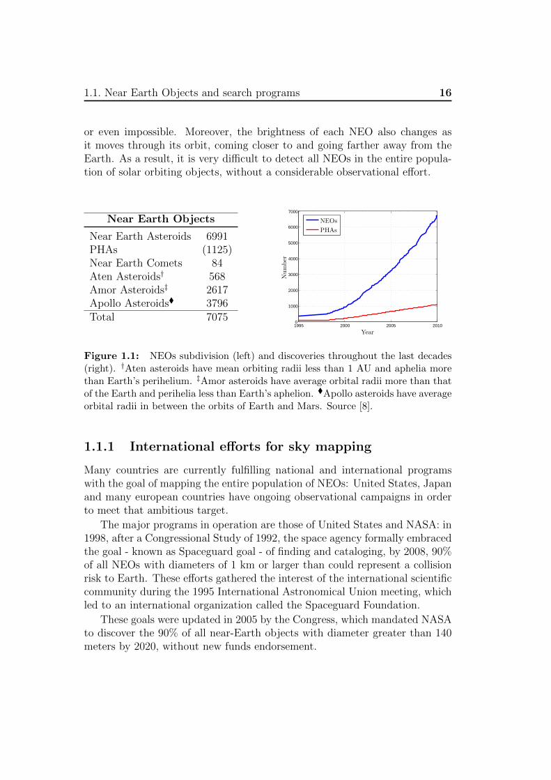
As of May 2010, 7075 NEOs have been discovered: among them, 84 near-Earth Comets (NECs) and 6991 near-Earth Asteroids (NEAs). 1125 of theprevious NEAs are catalogued as Potentially Hazardous Asteroids (PHAs),having the potential to make close approaches to the Earth and a size largeenough to cause significant regional or global damage in the event of impact.
Scientists’ ability to detect NEOs is dependent on how bright each individ-ual object appears in the sky, which depends primarily on its distance fromEarth, size, albedo and its location relative to the Sun. The observation ofNEOs that appear very close to the Sun when viewed from Earth is difficult
1An Astronomical Unit (AU) is the mean distance between the Sun and the Earth, i.e.149597870.7 km.
15
1.1. Near Earth Objects and search programs 16
or even impossible. Moreover, the brightness of each NEO also changes asit moves through its orbit, coming closer to and going farther away from theEarth. As a result, it is very difficult to detect all NEOs in the entire popula-tion of solar orbiting objects, without a considerable observational effort.
Near Earth Objects
Near Earth Asteroids 6991PHAs (1125)Near Earth Comets 84Aten Asteroids† 568Amor Asteroids‡ 2617Apollo Asteroids 3796Total 7075
1995 2000 2005 20100
1000
2000
3000
4000
5000
6000
7000
Year
Num
ber
NEOs
PHAs
Figure 1.1: NEOs subdivision (left) and discoveries throughout the last decades(right). †Aten asteroids have mean orbiting radii less than 1 AU and aphelia morethan Earth’s perihelium. ‡Amor asteroids have average orbital radii more than thatof the Earth and perihelia less than Earth’s aphelion. Apollo asteroids have averageorbital radii in between the orbits of Earth and Mars. Source [8].
1.1.1 International efforts for sky mapping
Many countries are currently fulfilling national and international programswith the goal of mapping the entire population of NEOs: United States, Japanand many european countries have ongoing observational campaigns in orderto meet that ambitious target.
The major programs in operation are those of United States and NASA: in1998, after a Congressional Study of 1992, the space agency formally embracedthe goal - known as Spaceguard goal - of finding and cataloging, by 2008, 90%of all NEOs with diameters of 1 km or larger than could represent a collisionrisk to Earth. These efforts gathered the interest of the international scientificcommunity during the 1995 International Astronomical Union meeting, whichled to an international organization called the Spaceguard Foundation.
These goals were updated in 2005 by the Congress, which mandated NASAto discover the 90% of all near-Earth objects with diameter greater than 140meters by 2020, without new funds endorsement.
17 1. Introduction
NEOs institutions and search groups
Observation Catalog Coordination ResearchSpaceguard Foundation •NASA/JPL • • •NEODyS at Pisa U. • • •EARN •Minor Planet Center • •Catalina Sky Survey • • •LINEAR/MIT • •LONEOS† •NEAT/JPL‡ •JSGA • • •Asiago-DLRN •Campo ImperatoreH •Table Mountain Obs. •Kitt Peak National Obs. •Loomberah Obs. •
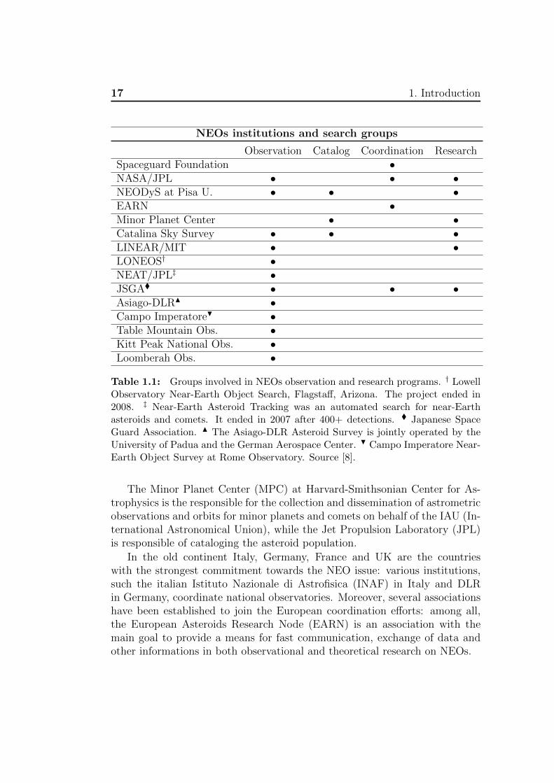
Table 1.1: Groups involved in NEOs observation and research programs. † LowellObservatory Near-Earth Object Search, Flagstaff, Arizona. The project ended in2008. ‡ Near-Earth Asteroid Tracking was an automated search for near-Earthasteroids and comets. It ended in 2007 after 400+ detections. Japanese SpaceGuard Association. N The Asiago-DLR Asteroid Survey is jointly operated by theUniversity of Padua and the German Aerospace Center. H Campo Imperatore Near-Earth Object Survey at Rome Observatory. Source [8].
The Minor Planet Center (MPC) at Harvard-Smithsonian Center for As-trophysics is the responsible for the collection and dissemination of astrometricobservations and orbits for minor planets and comets on behalf of the IAU (In-ternational Astronomical Union), while the Jet Propulsion Laboratory (JPL)is responsible of cataloging the asteroid population.
In the old continent Italy, Germany, France and UK are the countrieswith the strongest commitment towards the NEO issue: various institutions,such the italian Istituto Nazionale di Astrofisica (INAF) in Italy and DLRin Germany, coordinate national observatories. Moreover, several associationshave been established to join the European coordination efforts: among all,the European Asteroids Research Node (EARN) is an association with themain goal to provide a means for fast communication, exchange of data andother informations in both observational and theoretical research on NEOs.
1.1. Near Earth Objects and search programs 18
1.1.2 Earth-based observatories
Earth-based telescopes, operating in various ranges of the electromagneticspectrum, are the most reliable, low-cost and versatile system to span wideportions of the celestial sphere in order to record the position of asteroids,comets and artificial objects.
Various observatories are operating nowadays to fulfill the tasks purposedby US Congress and approved by different associations and space agencies’panels. In Italy, the Campo Imperatore telescope system at Gran Sasso andthe Asiago-DLR observatory in the north of the peninsula, are the most activeproducers of astrometric data. International observatories are summarized inTable (1.1).
Two unmentioned examples in United States are the Arecibo and Gold-stone radar systems, which play a unique role in the characterization of NEOs,providing unmatched accuracy in orbit determination and offering insight intosize, shape, surface structure, and other properties for objects within theirlatitude coverage and detection range.
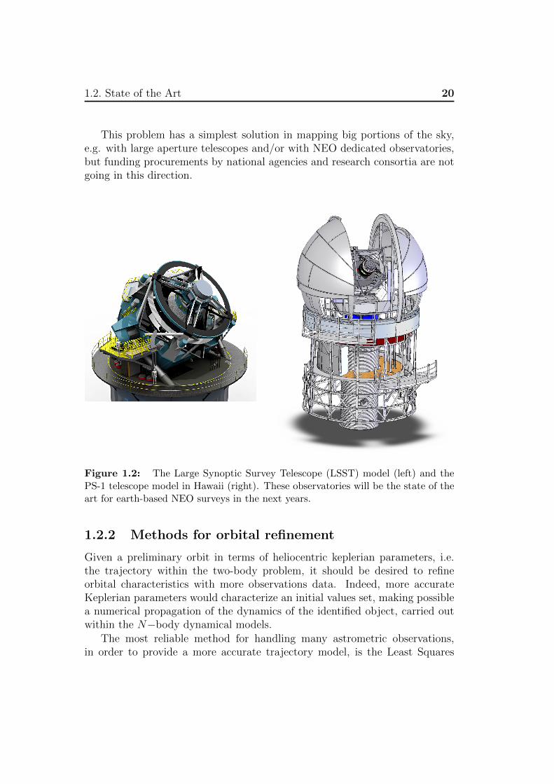
Regarding at the 2020 goals, two solution are underway: the constructionof the Large Synoptic Survey Telescope (LSST) in Chile, whose primary mirrorhas been cast and polished, but not been fully funded yet, and the PanoramicSurvey Telescope and Rapid Response System in Hawaii.
1.1.3 Space telescopes
Historically, the detection of asteroids and comets has been a prerogative ofEarth-based observatories and terrestrial telescopes, while the study of galaxiesand astrophysics in general was becoming a space-based activity, marking theboundaries between astrophysics and classical astronomy.
Despite this subdivision, that still today don’t lack of soundness, beingurged by a House of Representatives survey regarding the status of US NEO’sdetection programs in 2007, NASA officials purposed the use of the Wide-fieldInfrared Survey Explorer (WISE) spacecraft for NEOs detection targets.
WISE was launched in december 14, 2009, from Vandenberg Air Force Base,equipped with a 40 cm diameter Infrared (IR) telescope, whose detectors arecooled as cryogenic temperatures. By May 27, 2010, WISE discovered 12,141previously unknown asteroids, of which 64 were considered near-Earth, and11 new comets. At the end of the first phase of the mission, a total of 136new NEAs, PHAs and Comets were discovered. In October 2010, the NASAPlanetary Division saved the spacecraft from termination with a one monthprogram extension called Near-Earth Object WISE (NEOWISE). The focus of
19 1. Introduction
mission, ended at the end of january 2011, was to look for asteroids and cometsclose to Earth orbit, using the remaining post-cryogenic detection capability.
Moreover, a canadian-built microsatellite, Near-Earth-Object SurveillanceSatellite (NEOSSat), is designed to obtain observations on both human-madeand natural objects in near-Earth space. Its launch is planned for 2011. Atlast, AsteroidFinder, a DLR proposed satellite, is under construction and setfor launch in 2012, if confirmed by the german space agency.
1.2 State of the Art
1.2.1 Methods for preliminary orbital determination
The orbit of a celestial body, such as a comet or an asteroid around the Sun canbe firstly determined assuming the two-body dynamics, that means consideringthe dynamical effects of the main attractor only, i.e. the Sun-comet and theSun-asteroid systems.
Historically, the Gibbs method predicts an orbit using three position vec-tors, while another common method determines an orbit from angle and rangemeasurements. Indeed, Earth-based observatories and telescopes produce an-gular observations, making Gauss’ method (GM) the more suitable mathemat-ical method to provide preliminary orbital determination.
The Gauss Method computes the preliminary orbit of the unknown objectfrom a set I of three angular observations spaced by ∆t. These observationsare composed by two angles each, e.g. topocentric Right Ascension α anddeclination δ.
The way to detect NEOs is relatively simple and reliable: small portionsof sky ares scanned in visible, IR and microwave spectra and CCD technologyrecords data for automatic analysis of astrometric values. Notwithstanding,the difficulties in mapping NEOs are related to the possibility to perform aminimum of three observations of the same object with the proper timing, toimplement the classical Gauss method and consequently to rely on a prelimi-nary orbit2.
Moreover, the time steps between observations must be sufficiently elevatedrespect to the orbital period - that is unknown - to determine a reliable Gausssolution. This causes various problems in order to identity the sky positionswhere to detect the previous observed object.
2Preliminary or optimized asteroids’ data at Minor Planet Center or other DBs are inthe form of heliocentric Keplerian Elements.
1.2. State of the Art 20
This problem has a simplest solution in mapping big portions of the sky,e.g. with large aperture telescopes and/or with NEO dedicated observatories,but funding procurements by national agencies and research consortia are notgoing in this direction.
Figure 1.2: The Large Synoptic Survey Telescope (LSST) model (left) and thePS-1 telescope model in Hawaii (right). These observatories will be the state of theart for earth-based NEO surveys in the next years.
1.2.2 Methods for orbital refinement
Given a preliminary orbit in terms of heliocentric keplerian parameters, i.e.the trajectory within the two-body problem, it should be desired to refineorbital characteristics with more observations data. Indeed, more accurateKeplerian parameters would characterize an initial values set, making possiblea numerical propagation of the dynamics of the identified object, carried outwithin the N−body dynamical models.
The most reliable method for handling many astrometric observations,in order to provide a more accurate trajectory model, is the Least Squares
21 1. Introduction
method, described by Carl Friedrich Gauss around 1794. Given p−observationdata, i.e. Right Ascension and Declination angles, the method provides a bestfit in the least-squares sense, minimizing the sum of squared residuals, a resid-ual being the difference between an observed value and the fitted value providedby the two-body/N−body models.
An early demonstration of the strength of least-squares method came whenit was used to predict the future location of the newly discovered asteroid Ceres.On January 1, 1801, the Italian astronomer Giuseppe Piazzi discovered Ceresand was able to track its path for 40 days before it was lost. Based on this data,astronomers desired to determine the location of Ceres after it emerged frombehind the sun without solving the Kepler’s equations of planetary motion.The only predictions that successfully allowed Hungarian astronomer FranzXaver von Zach to relocate Ceres were those performed by Gauss using least-squares analysis.
1.3 Angles uncertainties and the gap through
successive observations
Preliminary orbit determination through Gauss method and classical orbitaloptimization, carried out by decades to provide best fittings, are nowadaysefficient and safe.
However, an evident difficulty for astronomers is given by the propagationof the astrometry errors, that evidently don’t permit to calculate a sufficientlyreliable preliminary orbit: indeed, the Gauss method would produce a set ofpreliminary Classical Orbital Elements (COE), affected by unknown errors.Being all astrometric angles potentially affected by errors, it is not efficientto calculate the next positions of the sky where the NEO should be, basingsolely on two-body propagation. This problem increases when a observation iscarried out with a small ∆t, characterizing a so-called ’short arc’ or ’too shortarc’.
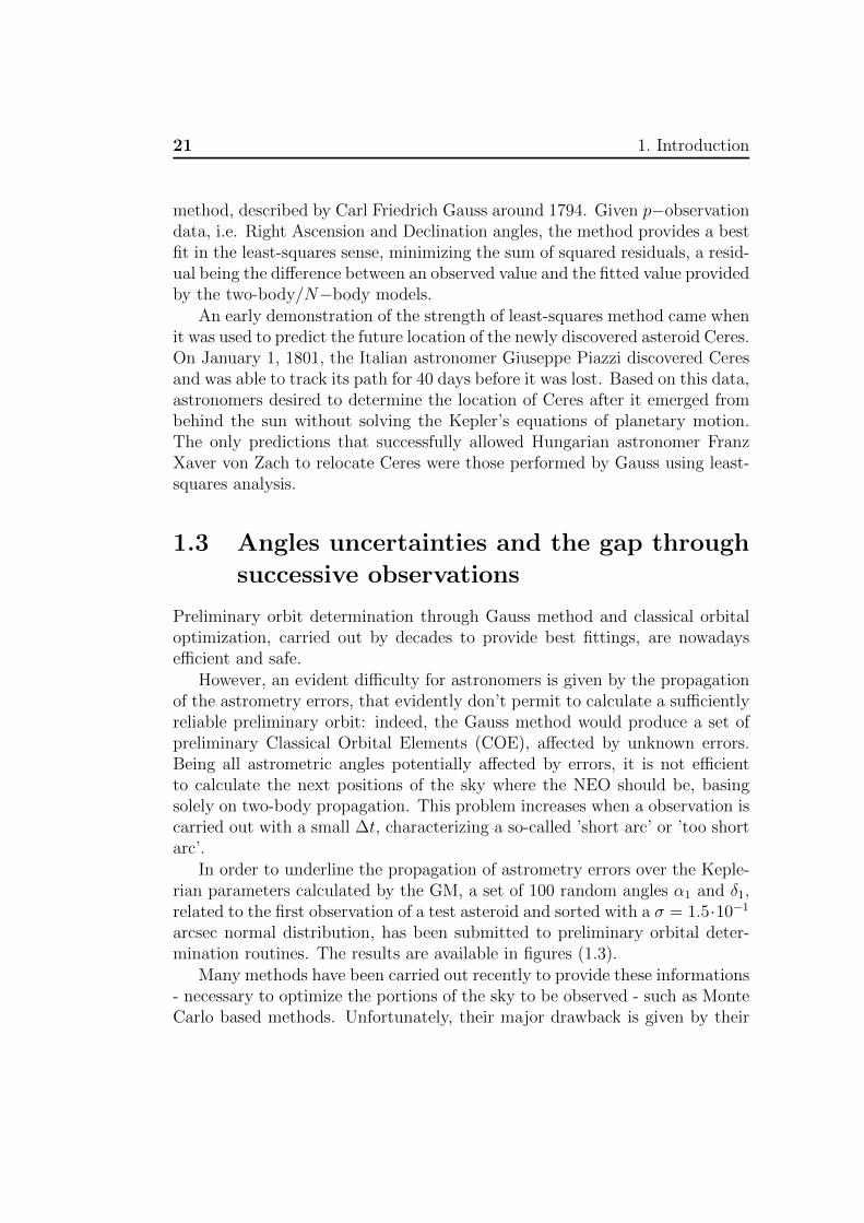
In order to underline the propagation of astrometry errors over the Keple-rian parameters calculated by the GM, a set of 100 random angles α1 and δ1,related to the first observation of a test asteroid and sorted with a σ = 1.5·10−1
arcsec normal distribution, has been submitted to preliminary orbital deter-mination routines. The results are available in figures (1.3).
Many methods have been carried out recently to provide these informations- necessary to optimize the portions of the sky to be observed - such as MonteCarlo based methods. Unfortunately, their major drawback is given by their
1.4. Proposed solution 22
high demanding computing effort.
0 20 40 60 80 1001
1.5
2
2.5
3
3.5
4
4.5
5
5.5
Initial perturbations ID
Sem
imajo
raxis
[AU
]
Perturbed data
Nominal solution
(a) Semimajor axis.
0 20 40 60 80 1000.72
0.74
0.76
0.78
0.8
0.82
0.84
0.86
0.88
0.9
Initial perturbations IDE
ccen
tric
ity
Perturbed data
Nominal solution
(b) Eccentricity.
0 20 40 60 80 100330
335
340
345
350
355
360
Initial perturbations ID
RA
AN
[deg
]
Perturbed data
Nominal solution
(c) Right Ascension of the Ascending Node.
0 20 40 60 80 1000
2
4
6
8
10
12
14
Initial perturbations ID
Incl
ination
[deg
]
Perturbed data
Nominal solution
(d) Inclination.
Figure 1.3: Evaluation of many Classical Orbital Elements calculated by theGauss Method with perturbed initial data in terms of σ normal probability distri-bution.
1.4 Proposed solution
An elegant solution based on Differential Algebraic (DA) techniques is investi-gated in this work to identify the so-called Virtual Asteroids (VAs), represent-ing the possible astrometric positions of the NEO associated to perturbationof the set I. These simulated VAs characterize a solution cloud in the celestialsphere, which is propagated with a DA-based Kepler’s equation to help theastronomers in detecting lost asteroids.
Differential Algebraic techniques have been developed by M.Berz at Michi-
23 1. Introduction
gan State University, to find an algebraic approach to solve parametric anddifferential problems. More specifically, the solution manifold of the problemis decribed by n−dimensional high-order Taylor polynomials. This method isimplemented in the programming language COSY INFINITY.
Sky mapping
(α, δ, spectrum) recording
Known?yes
Optimization
no
Attending new observations
Orbit known?
yes
no
Solve Gauss method
DA-basedVirtual Asteroids
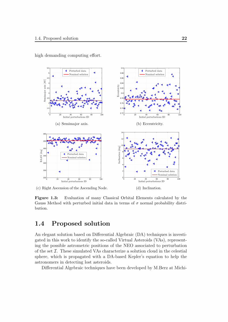
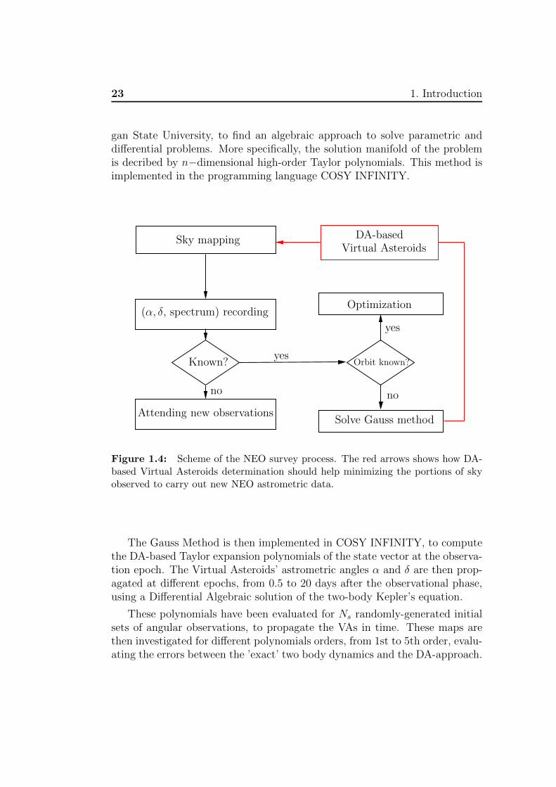
Figure 1.4: Scheme of the NEO survey process. The red arrows shows how DA-based Virtual Asteroids determination should help minimizing the portions of skyobserved to carry out new NEO astrometric data.
The Gauss Method is then implemented in COSY INFINITY, to computethe DA-based Taylor expansion polynomials of the state vector at the observa-tion epoch. The Virtual Asteroids’ astrometric angles α and δ are then prop-agated at different epochs, from 0.5 to 20 days after the observational phase,using a Differential Algebraic solution of the two-body Kepler’s equation.
These polynomials have been evaluated for Ns randomly-generated initialsets of angular observations, to propagate the VAs in time. These maps arethen investigated for different polynomials orders, from 1st to 5th order, evalu-ating the errors between the ’exact’ two body dynamics and the DA-approach.
1.5. Presentation plan 24
1.5 Presentation plan
The thesis work is organized in six chapters. Arguments treated in each chapterare summed up as follows.
Chapter 1
Introduction to Near Earth Objects’ surveys and to the methods for orbitaldetermination and refinement.
Chapter 2
The Gauss Method for preliminary orbital determination and its iterative im-provement. Evaluation of convergence properties respect to ∆t between ob-servations.
Chapter 3
Fundamentals of Differential Algebra, with properties and approaches to solveimplicit equations and parametric equations.
Chapter 4
Application of Differential Algebraic techniques to evaluate the high orderexpansion of the orbital determination problem. Particular attention is givento the evaluation of the errors between the two-body dynamical model and theDifferential Algebraic approach.
Chapter 5
High order mapping of Virtual Asteroids. The astrometric positions of eachVirtual Asteroid are propagated for different epochs as up 5th polynomialorder.
Chapter 6
Conclusions and Future work.
Chapter 2
The Gauss method for orbitaldetermination
The Gauss method takes its name and origin from the german mathematicianKarl Friedrich Gauss who, in 1801, formulated an elegant analytical solutionin order to solve the orbital determination of Ceres, the dwarf planet orbitingin the Main Asteroid Belt and discovered by Giuseppe Piazzi in the same year.
This method, with successive refinements and iterative improvements, isused nowadays to determine an orbit from a set of three angular observations,i.e. when the number of the observations is too small to apply the moderntechniques of orbital optimization.
2.1 Dynamical framework and input data
Being the Gauss method a preliminary way to determine an orbit in space,it relies on some approximations. More specifically, the unknown object isassumed to orbit a main attractor, in the two-body dynamical framework; e.g.Sun-asteroid and Sun-comet systems.
The preliminary determination of an orbit in the two-body system requiressix independent parameters: these quantities can be the six classical orbitalelements; the orbital state vectors r and v ; the orbital energy ε, the angularmomentum h and the eccentricity vector e .
As with a telescope we must rely on measurements of two angles only, a min-imum of three observation is required to collect the six independent quantitiesneeded to predict the preliminary orbit. These two angles could be elevationand azimuth, geocentric Right Ascension and declination, or topocentric Right
25
2.1. Dynamical framework and input data 26
Ascension (RA) and declination (dec). The topocentric RA α and declinationδ are used in this work to simulate the observation angles.
The set of angles I needed for Gauss orbital determination is thus composedby
I = (α1, δ1)t1 , (α2, δ2)t2 , (α3, δ3)t3 , (2.1)
where (αi, δi)ti is the i−set of angles at observation time ti.
In case of topocentric angles, further information are needed in order tolocalize the observation site, such as geocentric coordinates of the Earth-basedtelescope. Moreover, the set I shall be precisely correlated to the observationtimes t1, t2, t3, usually expressed in Julian Date.
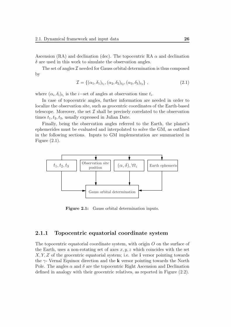
Finally, being the observation angles referred to the Earth, the planet’sephemerides must be evaluated and interpolated to solve the GM, as outlinedin the following sections. Inputs to GM implementation are summarized inFigure (2.1).
Gauss orbital determination
t1, t2, t3Observation site
position (α, δ), ∀ti Earth ephemeris
Figure 2.1: Gauss orbital determination inputs.
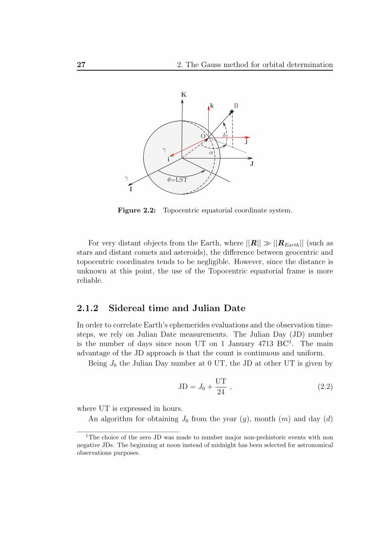
2.1.1 Topocentric equatorial coordinate system
The topocentric equatorial coordinate system, with origin O on the surface ofthe Earth, uses a non-rotating set of axes x, y, z which coincides with the setX, Y, Z of the geocentric equatorial system; i.e. the i versor pointing towardsthe γ- Vernal Equinox direction and the k versor pointing towards the NorthPole. The angles α and δ are the topocentric Right Ascension and Declinationdefined in analogy with their geocentric relatives, as reported in Figure (2.2).
27 2. The Gauss method for orbital determination
γ
K
J
I
γ
B
α
δO
θ=LST
j
k
i
Figure 2.2: Topocentric equatorial coordinate system.
For very distant objects from the Earth, where ||R|| ||REarth|| (such asstars and distant comets and asteroids), the difference between geocentric andtopocentric coordinates tends to be negligible. However, since the distance isunknown at this point, the use of the Topocentric equatorial frame is morereliable.
2.1.2 Sidereal time and Julian Date
In order to correlate Earth’s ephemerides evaluations and the observation time-steps, we rely on Julian Date measurements. The Julian Day (JD) numberis the number of days since noon UT on 1 January 4713 BC1. The mainadvantage of the JD approach is that the count is continuous and uniform.
Being J0 the Julian Day number at 0 UT, the JD at other UT is given by
JD = J0 +UT
24, (2.2)
where UT is expressed in hours.
An algorithm for obtaining J0 from the year (y), month (m) and day (d)
1The choice of the zero JD was made to number major non-prehistoric events with nonnegative JDs. The beginning at noon instead of midnight has been selected for astronomicalobservations purposes.
2.1. Dynamical framework and input data 28
triad, is based on Boulet formula
J0 = 367y− INT
7
[y + INT
(m+ 9
12
)]4
+ INT
(275m
9
)+d+ 1721013.5 ,
(2.3)where d ∈ [1, 31], m ∈ [1, 12] and y ∈ [1901, 2099].
A modern format is JD2000, defined to start noon on 1st January 2000,where JJD2000 = 2451545.0. The time in Julian centuries T0 is fundamental tofind the Greenwich sidereal time at 0 UT θG,0 with the Seidelmann formula
θG,0 = 100.4606184 + 36000.77 T0 + 0.0003879 T 20 − 2.583(10−8) T 3
0 , (2.4)
being T0 = (J0 − JJD2000)/36525.The Greenwich sidereal time at other UT is thus given by
θG = θG,0 + 360.985647UT
24. (2.5)
The Local Sidereal Time (LST) of the observation site is given by addingits East longitude Λ to the Greenwich sidereal time
θ = LST = θG + Λ . (2.6)
Finally, the asteroid ephemerides of MPC and Planetary ephemerides ofJPL are based on Mean Julian Date 2000 (MJD2000)
MJD2000 = J0 − 2451544.5 . (2.7)
2.1.3 Planetary ephemerides
Planetary ephemerides are required to determine the position of the Earth atthe observation times t1, t2, t3.
All routines implemented in this work use the JPL DE405 planetary ephemerides[9], whose reference system is the solar system barycenter equatorial J20002.These ephemerides are integrated through a variable-step Adams method, as-suming the VLBI (Very Long Baseline Interferometry) observations of the
2The barycenter of the Solar system is considered a quasi inertial frame of reference,defined by the measured positions of 212 extragalactic sources and known as InternationalCelestial Reference Frame (ICRF).
29 2. The Gauss method for orbital determination
Magellan spacecraft, in orbit around Venus, as initial conditions. The tabu-lated values of the integrated positions and velocities have a position accuracyof 1 km and validity in the range 2000-2100.
The position and velocity coefficients tabulated for the planet Earth atdiscrete JDs are interpolated through a Chebichev polynomial to determine thevalues of position and velocity vectors R⊕ and V ⊕ at specific JD/MJD2000.
2.2 Gauss method for Sun-orbiting asteroids
The Gauss method for orbital determination, named in honor of Carl FriedrichGauss (1777-1855), computes the keplerian orbit coherent to the I set of obser-vations. Since the orbits of asteroids and comets have the Sun as first attractor,it is natural to assume the classical orbital parameters respect to our star asultimate goals.
The vectors (Rt1obs,R
t2obs,R
t3obs) are the position vectors of the observation
site. The position vectors of the Earth (Rt1⊕ ,R
t2⊕ ,R
t3⊕) are calculated using the
ephemeris model mentioned above.
Let us define (ρ1, ρ2, ρ3), the cosine vectors from the observation site tothe observed object, obtained by measuring the set of topocentric angles in
ρ1 = cos δ1 cosα1I + cos δ1 sinα1J + sin δ1K
ρ2 = cos δ2 cosα2I + cos δ2 sinα2J + sin δ2K
ρ3 = cos δ3 cosα3I + cos δ3 sinα3J + sin δ3K .
(2.8)
It is clear that the position vectors of the observed body, with respect tothe Sun, (r 1, r 2, r 3), are obtained by
r 1 = Rt1
⊕ + Rt1obs + ρ1ρ1
r 2 = Rt2⊕ + Rt2
obs + ρ2ρ2
r 3 = Rt3⊕ + Rt3
obs + ρ3ρ3 ,
(2.9)
being (ρ1, ρ2, ρ3) the three slant ranges from the observation location to theobserved body.
2.2. Gauss method for Sun-orbiting asteroids 30
Asteroid path
Earth orbit
Sun ICRF
r 3
r 2
r 1
Rt3⊕
Rt2⊕
Rt1⊕
ρ1
ρ2
ρ3
t1
t2
t3
Z
γ
Y
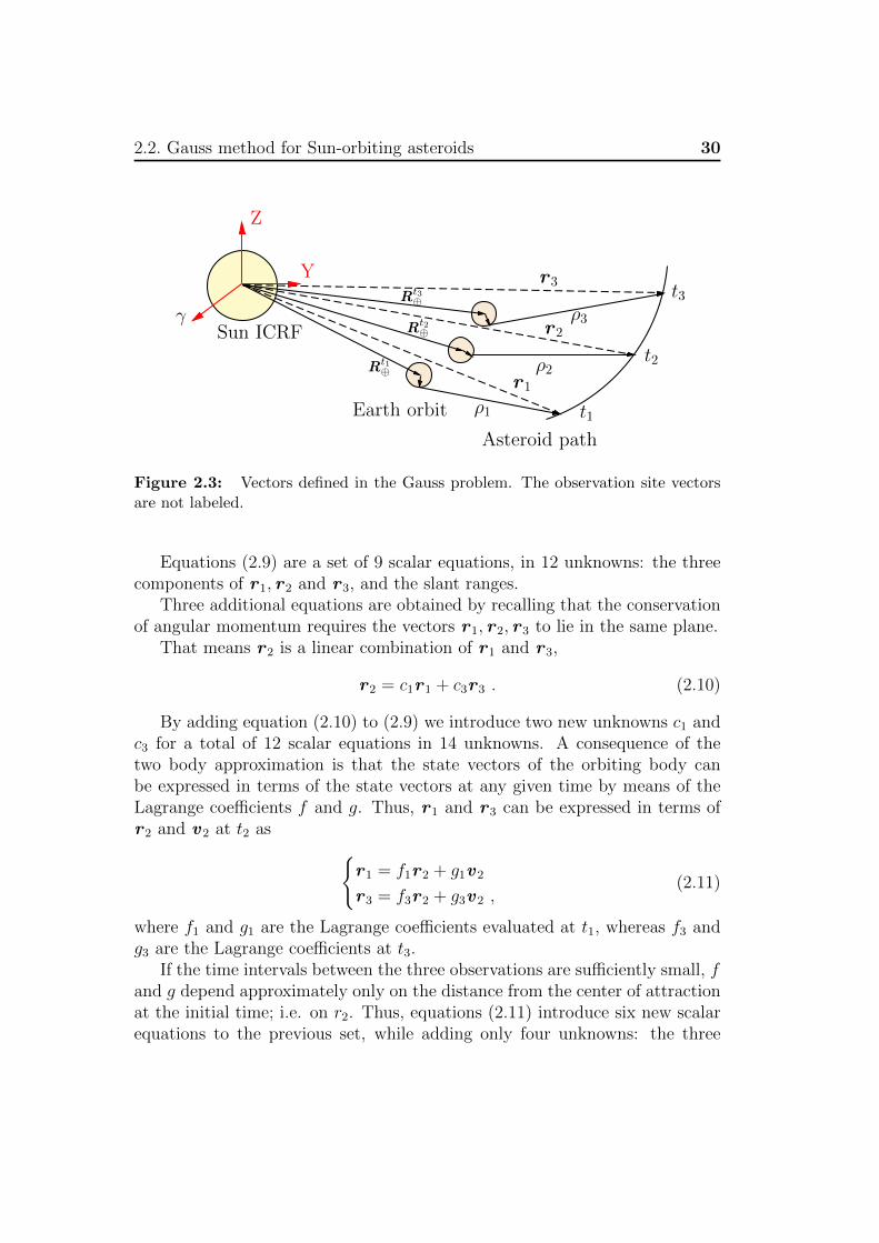
Figure 2.3: Vectors defined in the Gauss problem. The observation site vectorsare not labeled.
Equations (2.9) are a set of 9 scalar equations, in 12 unknowns: the threecomponents of r 1, r 2 and r 3, and the slant ranges.
Three additional equations are obtained by recalling that the conservationof angular momentum requires the vectors r 1, r 2, r 3 to lie in the same plane.
That means r 2 is a linear combination of r 1 and r 3,
r 2 = c1r 1 + c3r 3 . (2.10)
By adding equation (2.10) to (2.9) we introduce two new unknowns c1 andc3 for a total of 12 scalar equations in 14 unknowns. A consequence of thetwo body approximation is that the state vectors of the orbiting body canbe expressed in terms of the state vectors at any given time by means of theLagrange coefficients f and g. Thus, r 1 and r 3 can be expressed in terms ofr 2 and v 2 at t2 as
r 1 = f1r 2 + g1v 2
r 3 = f3r 2 + g3v 2 ,(2.11)
where f1 and g1 are the Lagrange coefficients evaluated at t1, whereas f3 andg3 are the Lagrange coefficients at t3.
If the time intervals between the three observations are sufficiently small, fand g depend approximately only on the distance from the center of attractionat the initial time; i.e. on r2. Thus, equations (2.11) introduce six new scalarequations to the previous set, while adding only four unknowns: the three
31 2. The Gauss method for orbital determination
components of v 2 and the radius r2. In conclusion we have a set of 18 equations.The problem of the preliminary orbital determination from three observations,with 18 equations and 18 unknowns, is well posed.
The ultimate objective is to determine the state vectors r 2 and v 2 at theintermediate time t2. Solving equation (2.10) for c1 and c3 and taking the crossproduct of each term of this equation with r 3, yields
r 2 × r 3 = c1(r 1 × r 3) + c3(r 3 × r 3) . (2.12)
Since r 3 × r 3 = 0, equation (2.12) reduces to
r 2 × r 3 = c1(r 1 × r 3) . (2.13)
Taking the dot product of this result with r 1 × r 3 and solving for c1 yields
c1 =(r 2 × r 3) · (r 1 × r 3)
||r 1 × r 3||2. (2.14)
Similarly, solving equation (2.10) for c1 and c3 and taking the cross productof each term of this equation with r 1 yields
r 2 × r 1 = c1(r 1 × r 1) + c3(r 3 × r 1) . (2.15)
Since r 1 × r 1 = 0, taking the dot product of each term of (2.15) with r 1 × r 3
and solving for c3 reads
c3 =(r 2 × r 1) · (r 3 × r 1)
||r 1 × r 3||2. (2.16)
Using equation (2.11), the cross product r 1 and r 3 reads
r 1×r 3 = (f1r 2+g1v 2)×(f3r 2+g3v 2) = f1g3(r 2×v 2)+f3g1(v 2×r 2) . (2.17)
By introducing the angular momentum h = r 2 × v 2, which is constant inthe two-body problem, we obtain
r 1 × r 3 = (f1g3 − f3g1)h (2.18)
and||r 1 × r 3||2 = (f1g3 − f3g1)2h2 . (2.19)
Similarly,r 2 × r 3 = r 2 × (f3r 2 + g3v 2) = g3h (2.20)
2.2. Gauss method for Sun-orbiting asteroids 32
r 2 × r 1 = r 2 × (f1r 2 + g1v 2) = g1h . (2.21)
Substituting equations (2.18), (2.19) and (2.20) into (2.14) leads to
c1 =g3
f1g3 − f3g1, (2.22)
while substituting equations (2.18), (2.19) and (2.21) into (2.16) leads to
c3 = − g1f1g3 − f3g1
. (2.23)
With these substitutions, the expression of r 2 = c1r 1 + c3r 3 is now exclu-sively expressed in terms of the Lagrange functions f and g. Unfortunatelyit is necessary to make some approximations in order to easily calculate thesecoefficients [10].
Assuming that the times between the three observations are small3 andintroducing
τ1 = t1 − t2 < 0 τ3 = t3 − t2 > 0 , (2.24)
as the time intervals between the successive measurements, we can use theseries expressions for the Lagrange coefficients f and g. Following [1], up toorder two for f and three for g, we have
f1 ≈ 1− µ
2r32τ 21 f3 ≈ 1− µ
2r32τ 23 (2.25)
g1 ≈ τ1 −µ
6r32τ 31 g3 ≈ τ3 −
µ
6r32τ 33 . (2.26)
Using (2.25) and (2.26) the denominator of (2.22) and (2.23) can be ex-pressed as
f1g3 − f3g1 =
(1− µ
2r32τ 21
)(τ3 −
µ
6r32τ 33
)−(
1− µ
2r32τ 23
)(τ1 −
µ
6r32τ 31
)(2.27)
and expanding the right side
f1g3 − f3g1 ≈ (τ3 − τ1)−µ
6r32(τ3 − τ1)3 +
µ2
12r62(τ 21 τ
33 − τ 31 τ 23 ) . (2.28)
Retaining terms of at most third order in the time intervals τ1 and τ3 anddefining
τ = τ3 − τ1 > 0 (2.29)
3A quantitative study of the Gauss method’s reliability with small time steps betweenobservations will be carried out at the end of this chapter.
33 2. The Gauss method for orbital determination
reduces (2.28) to
f1g3 − f3g1 ≈ τ − µ
6r32τ 3 . (2.30)
This leads to
c1 =g3
f1g3 − f3g1≈τ3 −
µ
6r32τ 33
τ − µ
6r32τ 3
=τ3τ
(1− µ
6r32τ 23
)(1− µ
6r32τ 2)−1
. (2.31)
Linearizing the last term in the right side as reported in [1] and neglectingterms of order higher than τ 2, the mentioned expression becomes(
1− µ
6r32τ 2)−1≈ 1 +
1
6
µ
r32τ 2 . (2.32)
Hence, equation (2.31) reduces to
c1 ≈τ3τ
[1 +
1
6
µ
r32(τ 2 − τ 23 )
](2.33)
and in the same way the expression of c3 can be expressed as
c3 ≈ −τ1τ
[1 +
1
6
µ
r32(τ 2 − τ 21 )
]. (2.34)
The next stage is to express the slant ranges ρ1, ρ2 and ρ3 in terms of c1and c3. In order to pursue this task, we resume equation (2.9) and simplify thenotation posing Ri = Rti
⊕ + Rtiobs; i.e. defining the vector from the center of
the Sun to the observation site. We then substitute equation (2.9) into (2.10)
R2 + ρ2ρ2 = c1(R1 + ρ2ρ1) + c3(R3 + ρ2ρ3) (2.35)
and rearrange it into the form
c1ρ1ρ1 − ρ2ρ2 + c3ρ3ρ3 = −c1R1 + R2 − c3R3 . (2.36)
The dot product of both sides of equation (2.36) with appropriate vectorsis useful to isolate the slant ranges. To isolate ρ1 we take the dot product ofeach term with ρ2 × ρ3
c1ρ1ρ1 · (ρ2 × ρ3)− ρ2ρ2 · (ρ2 × ρ3) + c3ρ3ρ3 · (ρ2 × ρ3) = (2.37)
= −c1R1 · (ρ2 × ρ3) + R2 · (ρ2 × ρ3)− c3R3 · (ρ2 × ρ3)
2.2. Gauss method for Sun-orbiting asteroids 34
Let us defineD0 = ρ1 · (ρ2 × ρ3) ,
and assume D0 6= 0, which means that ρ1, ρ2 and ρ3 do not lie in thesame plane, since ρ2 · (ρ2 × ρ3) = ρ3 · (ρ2 × ρ3) = 0. Equation (2.37) can berewritten in terms of ρ1
ρ1 =1
D0
(−D11 +
1
c1D21 −
c3c1D31
), (2.38)
where
D11 = R1 · (ρ2 × ρ3) D21 = R2 · (ρ2 × ρ3) D31 = R3 · (ρ2 × ρ3) .
Similarly, by taking the dot product of equation (2.36) with ρ1 × ρ3 andρ1 × ρ2, the following expressions for ρ2 and ρ3 are obtained
ρ2 =1
D0
(−c1D12 +D22 − c3D32) (2.39)
and
ρ3 =1
D0
(−c1c3D13 +
1
c3D23 −D33
), (2.40)
where
D12 = R1 · (ρ1 × ρ3) D22 = R2 · (ρ1 × ρ3) D32 = R3 · (ρ1 × ρ3)
and
D13 = R1 · (ρ1 × ρ2) D23 = R2 · (ρ1 × ρ2) D33 = R3 · (ρ1 × ρ2) .
Substituting the expressions of c1 and c3 into equation (2.39), the approx-imate slant range ρ2 is given by
ρ2 = A+µB
r32, (2.41)
where A,B = f(Dij, τ, τ1, τ3) reads
A =1
D0
(−D12
τ3τ
+D22 +D32τ1τ
)(2.42)
and
B =1
6D0
(D12(τ
23 − τ 2)
τ3τ
+D32(τ2 − τ 21 )
τ1τ
). (2.43)
35 2. The Gauss method for orbital determination
Therefore, making the same substitutions in (2.38) and in (2.40) leads tothe approximate formulas for the remaining slant ranges
ρ1 =1
D0
6
(D31
τ1τ3
+D21τ
τ3
)r32 + µD31(τ
2 − τ 21 )τ1τ3
6r32 + µ(τ 2 − τ 23 )−D11
(2.44)
and
ρ3 =1
D0
6
(D13
τ3τ1−D23
τ
τ1
)r32 + µD13(τ
2 − τ 23 )τ3τ1
6r32 + µ(τ 2 − τ 23 )−D33
. (2.45)
Equation (2.41) is a relation between the slant range ρ2 and the heliocentricradius of the observed object at time t2, r2. Another relation linking ρ2 andr2 is equation (2.9), rearranged in the form
r 2 · r 2 = (R2 + ρ2ρ2) · (R2 + ρ2ρ2) (2.46)
or
r22 = ρ22 + 2Eρ2 +R22 with E = R2 · ρ2 . (2.47)
Finally, substituting equation (2.41) into (2.47) gives
r22 =
(A+
µB
r32
2)+ 2C
(A+
µB
r32
)+R2
2 , (2.48)
known as the Eighth order polynomial of Gauss orbital determination
r82 + ar62 + br32 + c = 0 , (2.49)
where
a = −(A2 + 2AE +R22) b = −2µB(A+ E) c = −µ2B2 .
2.2. Gauss method for Sun-orbiting asteroids 36
Calculate the time intervals
τ, τ1, τ3
Calculate the dot product creating
D0, Di,j A,B
Calculate the polynomial coefficients to form
r82 + ar6
2 + br32 + c = 0
Data inputs ∀ti = 1...3
Ri⊕ tiRi
obs (α, δ)i
8 roots r2Complex
roots
Real
negative
Real positive roots
Slant ranges ρi r i
Lagrange coefff1, g1, f3, g3
v 2 and Keplerian elements
2
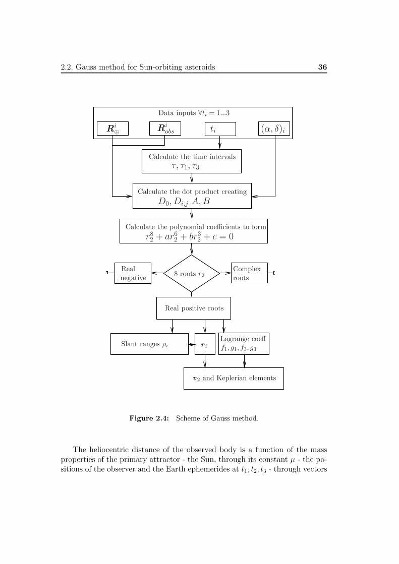
Figure 2.4: Scheme of Gauss method.
The heliocentric distance of the observed body is a function of the massproperties of the primary attractor - the Sun, through its constant µ - the po-sitions of the observer and the Earth ephemerides at t1, t2, t3 - through vectors
37 2. The Gauss method for orbital determination
Ri, embedded into Dijs - the cosine vectors ρi - through Dijs - and the timebetween the observations in A and B.
2.2.1 The Eighth order polynomial and the algorithmicflow
The eighth order polynomial (2.49) has eight solutions
r(i)2 ∈ C with i = 1...8 .
However, only the real solutions are of interest, representing a positive distance,i.e. the Euclidean norm of r 2. Moreover, with the subsequent calculation ofthe state vectors at t2 and the Classical Orbital Elements (COE), the ellipticaltrajectories only, respect to the Sun, must be taken into account. In facthyperbolic orbits do not characterize classical NEOs and NEAs.
Substituting r2 into equations (2.41), (2.44) and (2.45) we obtain the slantranges values, while equation (2.9) gives the heliocentric position vectors ofthe observed body. Once r 2 is known, v 2 can be calculated. Solving (2.11a)for r 2
r 2 =1
f1r 1 −
g1f1v 2 (2.50)
and substituting r 2 into (2.11b) yields
v 2 =1
f1g3 − f3g1(−f3r 1 + f1r 3) . (2.51)
The resulting heliocentric state vectors (r 2, v 2) can be used to calculatethe preliminary Keplerian elements of the observed asteroid or comet.
Figure (2.4) summarizes the algorithmic flow to calculate the preliminarystate vectors starting from a set of three observations.
2.2.2 Iterative improvement with Universal formulation
An iterative improvement of the previous method could revise the values of theslant ranges ρ1, ρ2, ρ3 and the state vectors using the Universal formulation forthe Lagrange coefficients f and g. As indicated in [?], the Universal formulationis more reliable and efficient from a computational viewpoint.
This formulation is based on a universal anomaly χ. Being t0 the timewhen this anomaly is zero, the value of χ at t0 + ∆t is found by the iterative
2.2. Gauss method for Sun-orbiting asteroids 38
solution of the universal Kepler’s equation
√µ∆t =
r0vr0√µχ2C(αχ2) + (1− αr0)χ3S(αχ2) + r0χ , (2.52)
where r0 and vr0 are the radius and the radial velocity at t0 and α is thereciprocal of the semimajor axis4 a
α =1
a. (2.53)
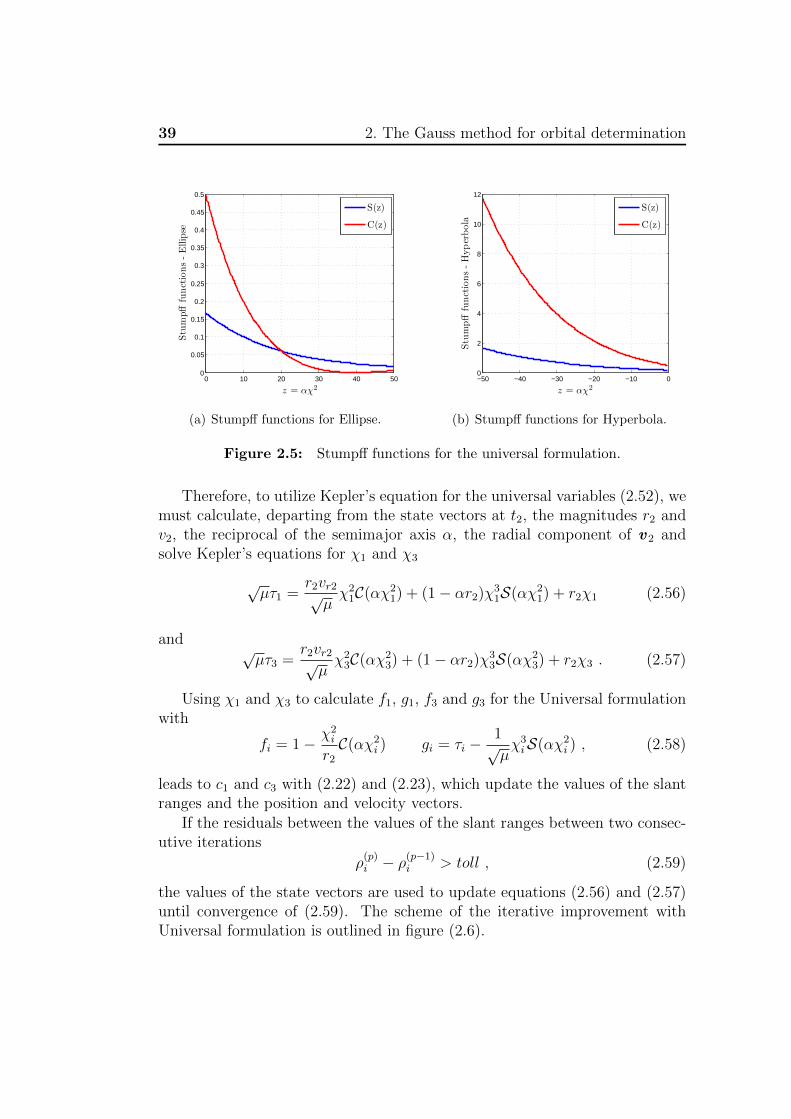
Being αχ2 dimensionless, C(αχ2) and S(αχ2) are known as Stumpff func-tions, defined by the following series,
S(z) =∞∑k=0
(−1)kzk
(2k + 3)!C(z) =
∞∑k=0
(−1)kzk
(2k + 2)!, (2.54)
with z = αχ2.
For the implementation of the Stumpff functions the following expressions,related to the circular and hyperbolic trigonometric functions, are more effi-cient:
S(z) =
√z − sin
√z
(√z)3
sinh√−z −√−z(√−z)3
1
6
C(z) =
1− cos√z
zz > 0
cosh√−z − 1
−z z < 0
1
2z = 0 ,
(2.55)
with z > 0 for ellipses, z < 0 for hyperbolas and z = 0 for parabolas.
4α > 0 for ellipses, α < 0 for hyperbolas and zero for parabolas.
39 2. The Gauss method for orbital determination
0 10 20 30 40 500
0.05
0.1
0.15
0.2
0.25
0.3
0.35
0.4
0.45
0.5
z = αχ2
Stu
mpff
funct
ions
-E
llip
se
S(z)
C(z)
(a) Stumpff functions for Ellipse.
−50 −40 −30 −20 −10 00
2
4
6
8
10
12
z = αχ2
Stu
mpff
funct
ions
-H
yper
bola
S(z)
C(z)
(b) Stumpff functions for Hyperbola.
Figure 2.5: Stumpff functions for the universal formulation.
Therefore, to utilize Kepler’s equation for the universal variables (2.52), wemust calculate, departing from the state vectors at t2, the magnitudes r2 andv2, the reciprocal of the semimajor axis α, the radial component of v 2 andsolve Kepler’s equations for χ1 and χ3
√µτ1 =
r2vr2√µχ21C(αχ2
1) + (1− αr2)χ31S(αχ2
1) + r2χ1 (2.56)
and √µτ3 =
r2vr2√µχ23C(αχ2
3) + (1− αr2)χ33S(αχ2
3) + r2χ3 . (2.57)
Using χ1 and χ3 to calculate f1, g1, f3 and g3 for the Universal formulationwith
fi = 1− χ2i
r2C(αχ2
i ) gi = τi −1√µχ3iS(αχ2
i ) , (2.58)
leads to c1 and c3 with (2.22) and (2.23), which update the values of the slantranges and the position and velocity vectors.
If the residuals between the values of the slant ranges between two consec-utive iterations
ρ(p)i − ρ(p−1)i > toll , (2.59)
the values of the state vectors are used to update equations (2.56) and (2.57)until convergence of (2.59). The scheme of the iterative improvement withUniversal formulation is outlined in figure (2.6).
2.3. Limits and drawbacks of Gauss method 40
r 2, v 2 ⇒ r2, v2, α = 1/a, vr2
Gauss Method - first guess
Solving universal Kepler’s eqnfor χ1 and χ3 at t1 and t3
Use χ1 and χ3 to calculateLagrange coeff fi, gi via Stumpff fun’s
Update the values of the slant rangesρ1, ρ2, ρ3 and vectors r 1, r 2, r 3
v 2
ρ(p)i − ρ(p−1)i < toll
no
End
yes
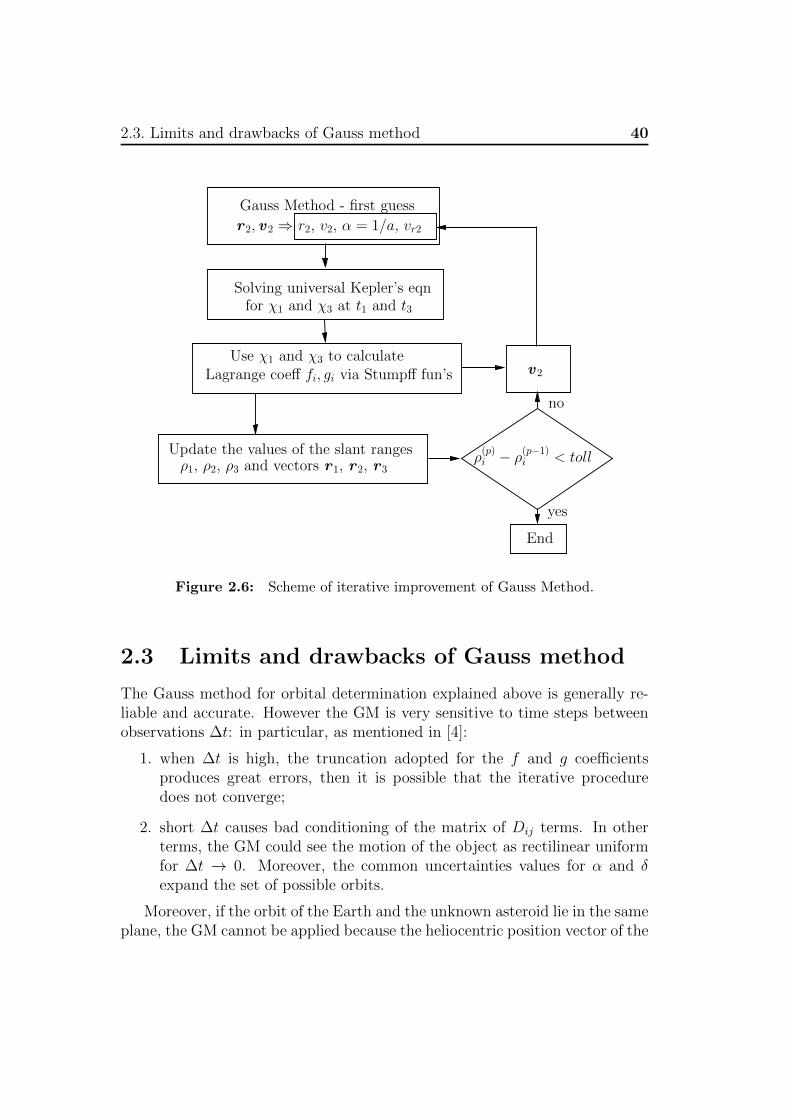
Figure 2.6: Scheme of iterative improvement of Gauss Method.
2.3 Limits and drawbacks of Gauss method
The Gauss method for orbital determination explained above is generally re-liable and accurate. However the GM is very sensitive to time steps betweenobservations ∆t: in particular, as mentioned in [4]:
1. when ∆t is high, the truncation adopted for the f and g coefficientsproduces great errors, then it is possible that the iterative proceduredoes not converge;
2. short ∆t causes bad conditioning of the matrix of Dij terms. In otherterms, the GM could see the motion of the object as rectilinear uniformfor ∆t → 0. Moreover, the common uncertainties values for α and δexpand the set of possible orbits.
Moreover, if the orbit of the Earth and the unknown asteroid lie in the sameplane, the GM cannot be applied because the heliocentric position vector of the
41 2. The Gauss method for orbital determination
asteroid and the Earth’s position vector do not allow do determine a reliableorbit causing the bad conditioning of the Dij terms. According to [4] orbitaldetermination methods devoted to coplanar orbits exist, but that eventualityis not common.
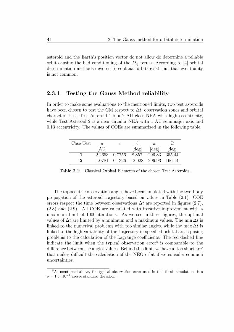
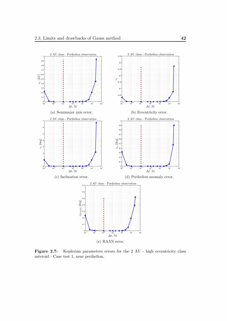
2.3.1 Testing the Gauss Method reliability
In order to make some evaluations to the mentioned limits, two test asteroidshave been chosen to test the GM respect to ∆t, observation zones and orbitalcharacteristics. Test Asteroid 1 is a 2 AU class NEA with high eccentricity,while Test Asteroid 2 is a near circular NEA with 1 AU semimajor axis and0.13 eccentricity. The values of COEs are summarized in the following table.
Case Test a e i ω Ω[AU] [deg] [deg] [deg]
1 2.2653 0.7756 8.857 296.83 355.442 1.0781 0.1326 12.028 296.93 166.14
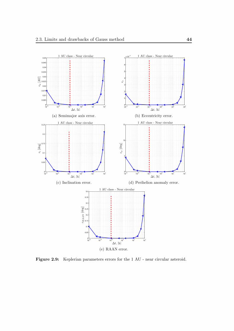
Table 2.1: Classical Orbital Elements of the chosen Test Asteroids.
The topocentric observation angles have been simulated with the two-bodypropagation of the asteroid trajectory based on values in Table (2.1). COEerrors respect the time between observations ∆t are reported in figures (2.7),(2.8) and (2.9). All COE are calculated with iterative improvement with amaximum limit of 1000 iterations. As we see in these figures, the optimalvalues of ∆t are limited by a minimum and a maximum values. The min ∆t islinked to the numerical problems with too similar angles, while the max ∆t islinked to the high variability of the trajectory in specified orbital areas posingproblems to the calculation of the Lagrange coefficients. The red dashed lineindicate the limit when the typical observation error5 is comparable to thedifference between the angles values. Behind this limit we have a ’too short arc’that makes difficult the calculation of the NEO orbit if we consider commonuncertainties.
5As mentioned above, the typical observation error used in this thesis simulations is aσ = 1.5 · 10−1 arcsec standard deviation.
2.3. Limits and drawbacks of Gauss method 42
10−3
10−2
10−1
100
101
102
103
0
0.1
0.2
0.3
0.4
0.5
0.6
0.7
0.8
0.9
1
Δt, [h]
ε a[A
U]
2 AU class - Perihelion observation
(a) Semimajor axis error.
10−3
10−2
10−1
100
101
102
103
0
0.05
0.1
0.15
0.2
0.25
0.3
0.35
Δt, [h]
ε e
2 AU class - Perihelion observation
(b) Eccentricity error.
10−3
10−2
10−1
100
101
102
103
0
1
2
3
4
5
6
7
Δt, [h]
ε i[d
eg]
2 AU class - Perihelion observation
(c) Inclination error.
10−3
10−2
10−1
100
101
102
103
0
0.1
0.2
0.3
0.4
0.5
0.6
0.7
0.8
0.9
1
Δt, [h]
ε ω[d
eg]
2 AU class - Perihelion observation
(d) Perihelion anomaly error.
10−3
10−2
10−1
100
101
102
103
0
0.1
0.2
0.3
0.4
0.5
0.6
0.7
Δt, [h]
ε RA
AN
[deg
]
2 AU class - Perihelion observation
(e) RAAN error.
Figure 2.7: Keplerian parameters errors for the 2 AU - high eccentricity classasteroid - Case test 1, near perihelion.
43 2. The Gauss method for orbital determination
10−4
10−2
100
102
104
0
0.5
1
1.5
2
2.5
3
3.5x 10
−3
Δt, [h]
ε a[A
U]
2 AU class - Aphelion observation
(a) Semimajor axis error.
10−4
10−2
100
102
104
0
0.5
1
1.5
2
2.5
3
3.5
4x 10
−3
Δt, [h]
ε e
2 AU class - Aphelion observation
(b) Eccentricity error.
10−4
10−2
100
102
104
0
0.5
1
1.5
2
2.5
3
3.5
4
4.5
5x 10
−3
Δt, [h]
ε i[d
eg]
2 AU class - Aphelion observation
(c) Inclination error.
10−4
10−2
100
102
104
0
0.02
0.04
0.06
0.08
0.1
0.12
0.14
Δt, [h]
ε ω[d
eg]
2 AU class - Aphelion observation
(d) Perihelion anomaly error.
10−4
10−2
100
102
104
0
0.02
0.04
0.06
0.08
0.1
0.12
0.14
0.16
0.18
0.2
Δt, [h]
ε RA
AN
[deg
]
2 AU class - Aphelion observation
(e) RAAN error.
Figure 2.8: Keplerian parameters errors for the 2 AU - high eccentricity classasteroid - Case test 1, near aphelion
2.3. Limits and drawbacks of Gauss method 44
10−3
10−2
10−1
100
101
102
0
0.005
0.01
0.015
0.02
0.025
0.03
0.035
0.04
0.045
0.05
Δt, [h]
ε a[A
U]
1 AU class - Near circular
(a) Semimajor axis error.
10−3
10−2
10−1
100
101
102
0
1
2
3
4
5
6
7x 10
−3
Δt, [h]
ε e
1 AU class - Near circular
(b) Eccentricity error.
10−3
10−2
10−1
100
101
102
0
0.05
0.1
0.15
0.2
0.25
Δt, [h]
ε i[d
eg]
1 AU class - Near circular
(c) Inclination error.
10−3
10−2
10−1
100
101
102
0
5
10
15
Δt, [h]
ε ω[d
eg]
1 AU class - Near circular
(d) Perihelion anomaly error.
10−3
10−2
10−1
100
101
102
0
0.05
0.1
0.15
0.2
0.25
0.3
0.35
0.4
Δt, [h]
ε RA
AN
[deg
]
1 AU class - Near circular
(e) RAAN error.
Figure 2.9: Keplerian parameters errors for the 1 AU - near circular asteroid.
Chapter 3
Fundamentals of DifferentialAlgebra
The modern so-called Differential Algebra (DA) took origin in the late 80’sby Martin Berz, professor of physics at the Michigan State University (MSU),during some efforts to find a robust and reliable mathematical tool to solvebeam physics problems, basing on Taylor polynomials algebra. The mainaspects of DA outlined in this chapter take advantages from his book ModernMap Methods in Particle Beam Physics.
3.1 Origin and similarities
Differential algebraic (DA) techniques find their origin in the attempt to solveanalytical problem by an algebraic approach. Historically, treatment of func-tions in numerics has been based on the treatment of numbers, and the classicalnumerical algorithms are based on the mere evaluation of functions at specificpoints. DA techniques are based on the observation that it is possible to ex-tract more information on a function rather than its mere values. The basicidea is to bring the treatment of functions and the operations on them to thecomputer environment in a similar way as the treatment of real numbers.
Referring to Figure (3.1), consider two real numbers a and b. In orderto operate on them in a computer environment, they are usually transformedin their floating point (FP) representation, a and b respectively. Then, givenany operation × in the set of real numbers, an adjoint operation ⊗ is definedin the set of FP numbers such that the diagram commutes. Consequently,transforming the real numbers a and b in their FP representation and operatingon them in the set of FP numbers returns the same result as carrying out the
45
3.1. Origin and similarities 46
operation in the set of real numbers and then transforming the achieved resultin its FP representation.
a, b ∈ R T−−−→ a, b ∈ FP×y ⊗
ya× b T−−−→ a⊗ b
f, gT−−−→ F,G
×y ⊗
yf × g T−−−→ F ⊗G
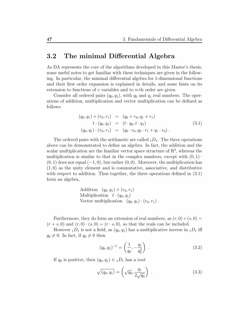
Figure 3.1: Analogy between the floating point representation of real numbers ina computer environment (left figure) and the introduction of the algebra of Taylorpolynomials in the differential algebraic framework (right figure).
In a similar way, suppose two sufficiently regular functions f and g aregiven. In the framework of differential algebra, the computer operates onthem using their Taylor series expansions, F and G respectively. Therefore,the transformation of real numbers in their FP representation is now substi-tuted by the extraction of the Taylor expansion of f and g. For each operationin the function space, an adjoint operation in the space of Taylor polynomi-als is defined such that the corresponding diagram commutes: extracting theTaylor expansions of f and g and operating on them returns the same resultas operating on f and g in the original space and then extracting the Tay-lor expansion of the resulting function. Differential algebra can be effectivelyimplemented in a computer environment.
In this way, the Taylor coefficients of a function can be obtained up to aspecified order n, along with the function evaluation, with a fixed amount ofeffort. The Taylor coefficients of order n for sums and product of functions, aswell as scalar products with reals, can be computed from those of summandsand factors; therefore, the set of equivalence classes of functions can be en-dowed with well-defined operations, leading to the so-called truncated powerseries algebra (TPSA).
Similarly to the algorithms for floating point arithmetic, the algorithm forfunctions followed, including methods to perform composition of functions,to invert them, to solve nonlinear systems explicitly, and to treat commonelementary functions. In addition to these algebraic operations, also the ana-lytic operations of differentiation and integration have been developed on thesefunction spaces, defining a differential algebraic structure.
47 3. Fundamentals of Differential Algebra
3.2 The minimal Differential Algebra
As DA represents the core of the algorithms developed in this Master’s thesis,some useful notes to get familiar with these techniques are given in the follow-ing. In particular, the minimal differential algebra for 1-dimensional functionsand their first order expansion is explained in details, and some hints on itsextension to functions of v variables and to n-th order are given.
Consider all ordered pairs (q0, q1), with q0 and q1 real numbers. The oper-ations of addition, multiplication and vector multiplication can be defined asfollows:
(q0, q1) + (r0, r1) = (q0 + r0, q1 + r1)
t · (q0, q1) = (t · q0, t · q1) (3.1)
(q0, q1) · (r0, r1) = (q0 · r0, q0 · r1 + q1 · r0) .
The ordered pairs with the arithmetic are called 1D1. The three operationsabove can be demonstrated to define an algebra. In fact, the addition and thescalar multiplication are the familiar vector space structure of R2, whereas themultiplication is similar to that in the complex numbers, except with (0, 1) ·(0, 1) does not equal (−1, 0), but rather (0, 0). Moreover, the multiplication has(1, 0) as the unity element and is commutative, associative, and distributivewith respect to addition. Thus together, the three operations defined in (3.1)form an algebra,
Addition (q0, q1) + (r0, r1)Multiplication t · (q0, q1)Vector multiplication (q0, q1) · (r0, r1) .
Furthermore, they do form an extension of real numbers, as (r, 0)+(s, 0) =(r + s, 0) and (r, 0) · (s, 0) = (r · s, 0), so that the reals can be included.
However 1D1 is not a field, as (q0, q1) has a multiplicative inverse in 1D1 iffq0 6= 0. In fact, if q0 6= 0 then
(q0, q1)−1 =
(1
q0,−q1
q20
). (3.2)
If q0 is positive, then (q0, q1) ∈ 1D1 has a root√(q0, q1) =
(√q0,
q12√q0
). (3.3)
3.2. The minimal Differential Algebra 48
One important property of this algebra is that it has an order compatiblewith its algebraic operations. Given two elements (q0, q1) and (r0, r1) in 1D1
it is defined
(q0, q1) < (r0, r1) if q0 < r0 or (q0 = r0 and q1 < r1) (3.4)
(q0, q1) > (r0, r1) if (r0, r1) < (q0, q1) (3.5)
(q0, q1) = (r0, r1) if q0 = r0 and q1 = r1 . (3.6)
And because for any two elements (q0, q1) and (r0, r1) only one of the threerelations holds, 1D1 is said totally ordered. The order is compatible with theaddition and multiplication; for all (q0, q1), (r0, r1), (s0, s1) ∈ 1D1, it follows
(q0, q1) < (r0, r1) ⇒ (q0, q1) + (s0, s1) < (r0, r1) + (s0, s1) (3.7)
and
(s0, s1) > (0, 0) = 0 ⇒ (q0, q1) · (s0, s1) < (s0, s1) · (s0, s1) . (3.8)
The number d = (0, 1) has the interesting property of being positive butsmaller than any positive real number: indeed
(0, 0) < (0, 1) < (r, 0) = r . (3.9)
For this reason d is called an infinitesimal or a differential. In fact, d is sosmall that its square vanishes in 1D1. Since for any (q0, q1) ∈ 1D1
(q0, q1) = (q0, 0) + (0, q1) = q0 + d · q1 , (3.10)
the first component is called the real part and the second component thedifferential part.
The algebra 1D1 becomes a differential algebra by introducing a map ∂from 1D1 to itself, and proving that the map is a derivation. Let’s define∂ : 1D1 → 1D1 by
∂(q0, q1) = (0, q1) . (3.11)
Note that
∂(q0, q1) + (r0, r1) = ∂(q0 + r0, q1 + r1) = (0, q1 + r1) (3.12)
= (0, q1) + (0, r1) = ∂(q0, q1) + ∂(r0, r1) (3.13)
49 3. Fundamentals of Differential Algebra
and
∂(q0, q1) · (r0, r1) = ∂(q0 · r0, q0 · r1 + r0 · q1) (3.14)
= (0, q0 · r1 + r0 · q1) (3.15)
= (0, q1) · (r0, r1) + (0, r1) · (q0, q1) (3.16)
= ∂(q0, q1) · (r0, r1) + (q0, q1) · ∂(r0, r1).(3.17)
This holds for all (q0, q1), (r0, r1) ∈ 1D1. Therefore ∂ is a derivation and(1D1, ∂) is a differential algebra.
3.2.1 1D1 and the automatic computation of derivatives
The most important aspect of 1D1 is that it allows the automatic computationof derivatives. As an example, assume to have two functions f and g; put theirvalues and their derivatives at the origin in the form
(f(0), f ′(0)) and (g(0), g′(0)) , (3.18)
as two vectors in 1D1, and consider the product
(f(0), f ′(0)) · (g(0), g′(0)) = (f(0) · g(0), f(0) · g′(0) + f ′(0) · g(0)) . (3.19)
As can be seen, if the derivative of the product f ·g is of interest, it has justto be looked at the second component of the resulting pair in (3.19); whereasthe first component gives the value of the product of the functions. Therefore,if two vectors contain the values and the derivatives of two functions, theirproduct contains the values and the derivatives of the product functions.
Defining the operation [ ] from the space of differential functions to 1D1 via
[f ] := (f(0), f ′(0)) (3.20)
it holds
[f + g] = [f ] + [g] (3.21)
[f · g] = [f ] · [g] (3.22)
and[1/g] = [1]/[g] = 1/[g] (3.23)
by using (3.2).This observation can be used to compute derivatives of many kinds of
functions algebrically by merely applying arithmetic rules on 1D1, starting from
3.2. The minimal Differential Algebra 50
the value and the derivative of the identity function. This will be important forthe calculation of the Taylor polynomials’ coefficients. Consider the example
f(x) =1
x+1
x
(3.24)
and its derivative
f ′(x) =(1/x2)− 1
(x+ 1/x)2. (3.25)
The function value and its derivative at the point x = 3 are
f(3) =3
10f ′(3) = − 2
25. (3.26)
Evaluating the function (3.24) at the ordered pair corresponding to the identityfunction, i.e. [x] = (x, 1), at the point 3, i.e. (3, 1) = 3 + d, yields
f(3, 1) =1
(3, 1) + 1/(3, 1)=
1
(3, 1) + (1/3,−1/9)(3.27)
=1
(10/3, 8/9)=
(3
10,−8
9/
100
9
)=
(3
10,− 2
25
). (3.28)
As can be seen, after the evaluation of the function, the real part of theresult is the value of the function at x = 3, whereas the differential part is thevalue of the derivative of the function at x = 3. This is simply justified byapplying the relations (3.21) and (3.23)
[f(x)] =
[1
x+ 1/x
]=
1
[x+ 1/x](3.29)
=1
[x] + [1/x]=
1
[x] + 1/[x](3.30)
= f([x]) . (3.31)
Since, for a real x, [x] = (x, 1) = x+d, and [f(x)] = (f(x), f ′(x)) apparently
(f(3), f ′(3)) = f((3 + d)) . (3.32)
The method can be generalized to allow the treatment of common intrinsicfunctions, like trigonometric or exponential functions, by setting
gi([f ]) = [gi(f)] (3.33)
51 3. Fundamentals of Differential Algebra
or
gi((q0, q1)) = (gi(q0), q1g′i(q0)) . (3.34)
By virtue of equations (3.1) and (3.34) any function f representable byfinitely many addictions, subtractions, multiplications, divisions, and intrinsicfunctions in 1D1 satisfies the important relationship
[f(x)] = f([x]) . (3.35)
Note that f(r + d) = f(r) + d · f ′(r) resembles
f(x+ ∆x) ≈ f(x) + ∆x · f ′(x) , (3.36)
in which the approximation becomes increasingly more refined for smaller ∆x.
3.3 The n-th order Differential Algebra
The algebra described in this section was introduced to compute the deriva-tives up to an order n of functions in v variables. Similarly as before, it isbased on considering the space Cn(Rv), i.e. the collection of n times continu-ously differentiable functions on Rv. On this space an equivalence relation isintroduced. For f and g ∈ Cn(Rv),
f =n g (3.37)
iff f(0) = g(0) and all the partial derivatives of f and g agree at 0 up to ordern.
The relation =n satisfies the followings
f =n f for all f ∈ Cn(Rv) (3.38)
f =n g ⇒ g =n f for all f, g ∈ Cn(Rv) (3.39)
f =n g and g =n h⇒ f =n h for all f, g, h,∈ Cn(Rv) . (3.40)
Thus, =n is an equivalence relation. All the elements that are related tof can be grouped together in one set, the equivalence class [f ] of the functionf . The resulting equivalence classes are often referred to as DA (DifferentialAlgebraic) vectors or DA numbers.
Intuitively, each of these classes is then specified by a particular collectionof partial derivatives in all v variables up to order n. This class is called nDv.

3.3. The n-th order Differential Algebra 52
If the values and the derivatives of two functions f and g are known, thecorresponding values and derivatives f+g and f ·g can be inferred. Therefore,the arithmetics on the classes nDv can be introduced via
[f ] + [g] = [f + g] (3.41)
t · [f ] = [t · f ] (3.42)
[f ] · [g] = [f · g] . (3.43)
Under these operations, nDv becomes an algebra.For each k ∈ 1, ..., v define the map ∂k from nDv to nDv for f via
∂k[f ] =
[pk ·
∂f
∂xk
], (3.44)
wherepk(x1, ..., xk) = xk (3.45)
projects out the k-th component of the identity function. It is easy to showthat, for all k = 1, ..., v and for all [f ], [g] ∈ nDv
∂k([f ] + [g]) = ∂k[f ] + ∂k[g] (3.46)
∂k([f ] · [g]) = [f ] · (∂k[g]) + (∂k[f ]) · [g] . (3.47)
Therefore, ∂k is a derivation for all k, and hence (nDv, ∂1, ..., ∂k) is a differ-ential algebra.
The dimension of nDv is now assessed. Define the special numbers dk asfollows:
dk = [xk] . (3.48)
Observe that f lies in the same class as its Taylor polynomial Tf of ordern around the origin; they have the same function values and derivatives up toorder n. Therefore
[f ] = [Tf ] . (3.49)
Denoting the Taylor coefficients of the Taylor polynomial Tf of f as cj1,...,jv ,it follows
Tf (x1, ..., xv) =∑
j1+...+jv≤ncj1,...,jv · xj11 · · · xjvv (3.50)
with
cji , ..., cjv =1
j1! · · · jv!· ∂j1+...+jvf
∂xj11 · · · ∂xjvv, (3.51)
53 3. Fundamentals of Differential Algebra
and thus
[f ] = [Tf ] =
[ ∑j1+...+jv≤n
cj1,...,jv · xj11 · · · xjvv
](3.52)
=∑
j1+...+jv≤ncj1,...,jv · dj11 · · · djvv , (3.53)
where, in the last step, the properties [a + b] = [a] + [b] and [a · b] = [a] · [b]have been used. Therefore, the set 1, dk : k = 1, 2, ..., v generates nDv,as any element of nDv can be obtained from 1 and the dk via addition andmultiplication.
Therefore, as an algebra, nDv has (v+1) generators, and the terms dj11 ···djvvform a basis for the vector space nDv. It can been demonstrated that thenumber of basic elements is (n+ v)!/(n!v!), which is the dimension of nDv.
Similarly to the structure 1D1, nDv can be ordered, and the terms dk, beingsmaller than any real number, are infinitely small or infinitesimal. Further-more, a fixed point theorem for contracting operators in nDv exists, whichenables the evaluation of square roots, the quotient, and the inversion of Tay-lor polynomials through iterative processes based on a finite number of steps.Once the function composition and the elementary functions, like trigonomet-ric or exponential functions, are introduced in nDv, the derivatives of anyfunction f belonging to Cn(Rv) can be computed up to order n in a fixedamount of effort by applying
[f(x1, ..., xv)] = f([x1, ..., xv]) = f(x1 + d1, ..., xv + dv) . (3.54)
The differential algebra sketched in this chapter was implemented by M.Berzand K.Makino in the software COSY INFINITY [3].
3.4 Solution of parametric implicit equations
DA techniques can be effectively used to identify the solution of paramet-ric implicit equations. Well-established numerical techniques (e.g. Newton’smethod) exist, which can identify the solution of a classical implicit equation
f(x) = 0 . (3.55)
Without loss of generality, suppose an explicit dependence on a parameter pcan be highlighted in the previous function f , which leads to the parametricimplicit equation
f(x, p) = 0 . (3.56)
3.4. Solution of parametric implicit equations 54
Suppose the previous equation is to be solved, whose solution is representedby the function x(p) returning the value of x solving (3.56) for any valueof the parameter p. Thus, the dependence of the solution of the implicitequation on the parameter p is of interest. DA techniques can effectivelyhandle the previous problem by identifying the function x(p) in terms of itsTaylor expansion with respect to the parameter p. The DA-based angorithmis presented in the followings for the solution of the scalar parametric implicitequation (3.56); the generalization to a system of parametric implicit equationsis straightforward.
The solution of (3.56) is sought, where sufficient regularity is assumed tocharacterize the function f , i.e. f ∈ Cn+1. This means that x(p) satisfying
f(x(p), p) = 0 (3.57)
is to be identified. The first step is to consider a reference value p0 of theparameter p and to compute the value of the solution x0 of the correspondingimplicit equation by means of a classical numerical method, e.g. Newton’smethod. The variable x and the parameter p are then initialized as n-th orderDA variables, i.e.
[x] = x0 + δx (3.58)
[p] = p0 + δp . (3.59)
A DA-based evaluation of the function f in (3.56) delivers the n-th orderexpansion of f with respect to x and p
δf =Mf (δx, δp) , (3.60)
where Mf denotes the Taylor map for f . Note that the map has no constantpart as x0 is the solution of the implicit equation for the nominal value of theparameter p0; thus δf represents the deviation of f from its reference value 0,resulting from deviations of x and p from x0 and p0. The map (3.60) is thenaugmented by introducing the map corresponding to the identity function onp, i.e. δp = Ip(δp), ending up with(
δfδp
)=
(Mf
Ip
)(δxδp
)(3.61)
The n-th order map (3.61) is inverted using COSY INFINITY built-intools, obtaining (
δxδp
)=
(Mf
Ip
)−1(δfδp
)(3.62)
55 3. Fundamentals of Differential Algebra
As the goal is to compute the n-th order Taylor expansion of the solutionmanifold x(p) of (3.56), the map (3.62) is evaluated for δf = 0:(
δxδp
)=
(Mf
Ip
)−1(0δp
). (3.63)
The first row of map (3.63) delivers
δx =Mδf=0(δp) , (3.64)
which is the n-th order Taylor expansion of the solution manifold, i.e.
δx = δx(δp) . (3.65)
For every value of p the approximate solution of f(x, p) = 0 can be easilycomputed by evaluating the Taylor polynomial at δp = p− p0.

Chapter 4
High order expansion of theorbital determination problem(Virtual Asteroids generation)
The main efforts towards the propagation of the so-called Virtual Asteroidsfind their rationales in the necessity of predicting the future positions of apotentially hazardous celestial body and, eventually, computing the Close Ap-proach Distance (CED) with respect to the Earth [6]. In fact, being the mea-surements of the NEO state affected by errors, the propagation of the set ofpossible trajectories associated to perturbed initial conditions yields a sort of’cloud’ of possible solutions, depending on the probability distribution of theinitial data.
Similarly, the errors on the astrometric angles of a newly-observed celestialbody limit the accuracy of the nominal orbit obtained with the GM, with thedrawback of losing the location of the body for days or months. Hence, the aimof this work is to find reliable admissible regions where a newly-observed NEOcan be observed in future times, in order to solve the gap between preliminaryorbit determination and orbital optimization1, as indicated in Figure (1.4).
Instead of using reliable but high-demanding Montecarlo simulations, Dif-ferential algebra is used here to compute high order Taylor expansions of thefuture positions of the NEO with respect to measure uncertainties. The VAsare then propagated by the simple evaluation of the resulting polynomials.
1Orbital optimization techniques compute a highly reliable orbit using least-squaresmethods. For this reason, the collection of many astrometric angles of an object is fun-damental to find an optimal solution.
57
4.1. High order Taylor polynomials for the generation of VAs 58
4.1 High order Taylor polynomials for the gen-
eration of VAs
Let us define the heliocentric state vectors of the newly-observed object, cal-culated with the GM, at time t2, r ∈ R3×1 and v ∈ R3×1. This vectors are thenominal solution of the orbital determination problem; i.e. let us write themas
r 0 =
rxryrz
∈ R3×1 v 0 =
vxvyvz
∈ R3×1 (4.1)
Moreover, we initialize them as n−th order DA-variables
rDA = [r ] = r 0 + δr (4.2)
vDA = [v ] = v 0 + δv . (4.3)
We define the nominal topocentric observation angles as algebraic vectors
α0 =
α1
α2
α3
∈ R3×1 δ0 =
δ1δ2δ3
∈ R3×1 . (4.4)
Then, we initialize them as DA variables
αDA = [α] = α0 + δα (4.5)
δDA = [δ] = δ0 + δδ . (4.6)
A DA-based Kepler’s ordinary differential equation developed by Armellinet Al [5] is now used to expand the flow of the two-body dynamics with rDA
and vDA as initial conditions. The flow is expanded forward and backwardwith a time step ∆t coherent with the Gauss Method solution, yielding rDA1
and rDA1 at t1 and rDA3 and rDA3 at t3. Then, the state vector’s polynomialsare used to compute the topocentric angles’ polynomials at the observationepochs αDA
c and δDAc .Similarly to section 3.4, a parametric implicit equation is now defined as
the difference between the astrometric angles calculated through the DA-basedKepler’s ODE and the values of (4.5) and (4.6). Thus we define the maps
∆α = αDAc − αDA =M∆α(δr , δv , δα, δδ) (4.7)
∆δ = δDAc − δDA =M∆δ(δr , δv , δα, δδ) . (4.8)

59 4. High order expansion of the orbital determination problem
The maps (4.7) and (4.8) are then augmented by introducing the mapcorresponding to the identity function on δα and δδ
∆α
∆δ
δαδδ
=
M∆α
M∆δ
IαIδ
δrδvδαδδ
. (4.9)
As the goal is to compute the n−th order Taylor expansion of the solutionmanifolds rDA = f(δα, δδ) and vDA = f(δα, δδ), the maps (4.9) are inverted
δrδvδαδδ
=
M∆α
M∆δ
IαIδ
−1
∆α
∆δ
δαδδ
. (4.10)
Then, because the errors ∆α and ∆δ must be zero, the inverted maps areevaluated for ∆α = 0 and ∆δ = 0
δrδvδαδδ
=
M∆α
M∆δ
IαIδ
−1
00δαδδ
. (4.11)
With the map inversion in (4.11), processed by COSY INFINITY built-intools, yields
δr = f(δα, δδ) (4.12)
δv = f(δα, δδ) , (4.13)
i.e. the solution expansion of the orbital determination problem, respect toany perturbed initial condition.
The state vectors are then computed with
rDA = r 0 + δr = r 0 + f(δα, δδ) (4.14)
vDA = v 0 + δv = v 0 + f(δα, δδ) . (4.15)
For every value of δα, δδ the approximate solution rDA and vDA can beeasily computed by evaluating the Taylor polynomial (4.14) and (4.15).
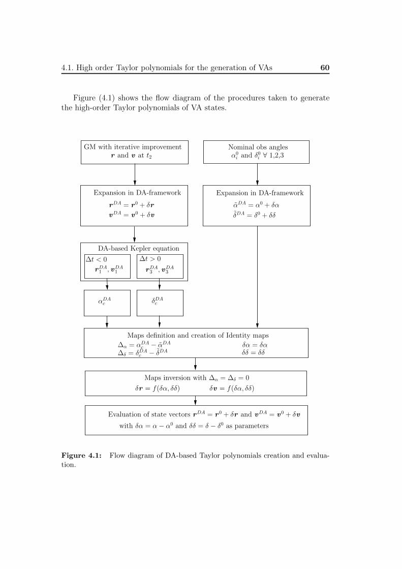
4.1. High order Taylor polynomials for the generation of VAs 60
Figure (4.1) shows the flow diagram of the procedures taken to generatethe high-order Taylor polynomials of VA states.
GM with iterative improvementr and v at t2
Expansion in DA-framework
rDA = r 0 + δr
vDA = v 0 + δv
Nominal obs anglesα0i and δ0i ∀ 1,2,3
Expansion in DA-framework
αDA = α0 + δα
δDA = δ0 + δδ
DA-based Kepler equation
∆t > 0∆t < 0
rDA1 , vDA1 rDA3 , vDA3
αDAc δDAc
Maps definition and creation of Identity maps
∆α = αDAc − αDA∆δ = δDAc − δDA
δα = δαδδ = δδ
Maps inversion with ∆α = ∆δ = 0
δr = f(δα, δδ) δv = f(δα, δδ)
Evaluation of state vectors rDA = r 0 + δr and vDA = v 0 + δv
with δα = α− α0 and δδ = δ − δ0 as parameters
2
Figure 4.1: Flow diagram of DA-based Taylor polynomials creation and evalua-tion.
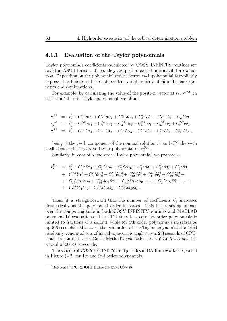
61 4. High order expansion of the orbital determination problem
4.1.1 Evaluation of the Taylor polynomials
Taylor polynomials coefficients calculated by COSY INFINITY routines aresaved in ASCII format. Then, they are postprocessed in MatLab for evalua-tion. Depending on the polynomial order chosen, each polynomial is explicitlyexpressed as function of the independent variables δα and δδ and their expo-nents and combinations.
For example, by calculating the value of the position vector at t2, rDA, in
case of a 1st order Taylor polynomial, we obtain
rDAx = r0x + Cr,x1 δα1 + Cr,x
2 δα2 + Cr,x3 δα3 + Cr,x
4 δδ1 + Cr,x5 δδ2 + Cr,x
6 δδ3
rDAy = r0y + Cr,y1 δα1 + Cr,y
2 δα2 + Cr,y3 δα3 + Cr,y
4 δδ1 + Cr,y5 δδ2 + Cr,y
6 δδ3
rDAz = r0z + Cr,z1 δα1 + Cr,z
2 δα2 + Cr,z3 δα3 + Cr,z
4 δδ1 + Cr,z5 δδ2 + Cr,z
6 δδ3 .
being r0j the j−th component of the nominal solution r 0 and Cr,ji the i−th
coefficient of the 1st order Taylor polynomial on rDAj .
Similarly, in case of a 2nd order Taylor polynomial, we proceed as
rDAj = r0j + Cr,j1 δα1 + Cr,j
2 δα2 + Cr,j3 δα3 + Cr,j
4 δδ1 + Cr,j5 δδ2 + Cr,j
6 δδ3
+ Cr,j7 δα2
1 + Cr,j8 δα2
2 + Cr,j9 δα2
3 + Cr,j10 δδ
21 + Cr,j
11 δδ22 + Cr,j
12 δδ23 +
+ Cr,j13 δα1δα2 + Cr,j
14 δα1δα3 + Cr,j15 δα2δα3 + ...+ Cr,j
i δαiδδi + ...+
+ Cr,j25 δδ1δδ2 + Cr,j
26 δδ1δδ3 + Cr,j27 δδ2δδ3 .
Thus, it is straightforward that the number of coefficients Ci increasesdramatically as the polynomial order increases. This has a strong impactover the computing time in both COSY INFINITY routines and MATLABpolynomials’ evaluations. The CPU time to create 1st order polynomials islimited to fractions of a second, while for 5th order polynomials increases asup 5-6 seconds2. Moreover, the evaluation of the Taylor polynomials for 1000randomly-generated sets of initial topocentric angles costs 2-3 seconds of CPU-time. In contrast, each Gauss Method’s evaluation takes 0.2-0.5 seconds, i.e.a total of 200-500 seconds.
The scheme of COSY INFINITY’s output files in DA-framework is reportedin Figure (4.2) for 1st and 2nd order polynomials.
2Reference CPU: 2.3GHz Dual-core Intel Core i5.
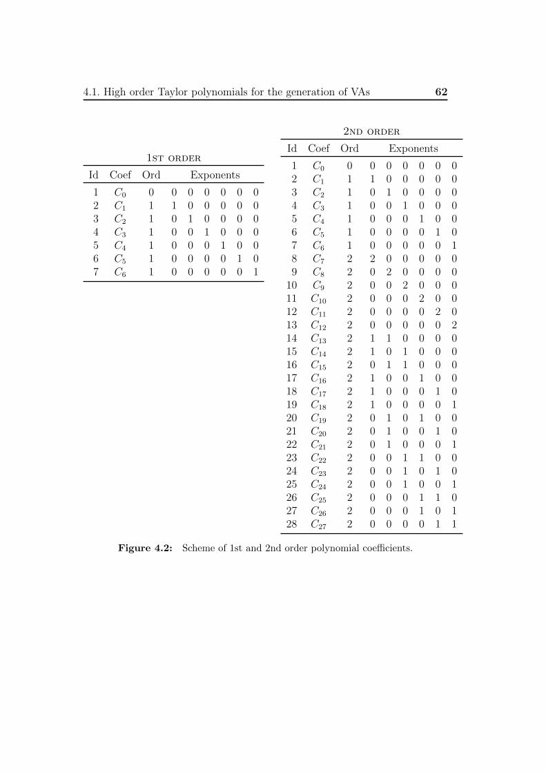
4.1. High order Taylor polynomials for the generation of VAs 62
1st order
Id Coef Ord Exponents
1 C0 0 0 0 0 0 0 02 C1 1 1 0 0 0 0 03 C2 1 0 1 0 0 0 04 C3 1 0 0 1 0 0 05 C4 1 0 0 0 1 0 06 C5 1 0 0 0 0 1 07 C6 1 0 0 0 0 0 1
2nd order
Id Coef Ord Exponents
1 C0 0 0 0 0 0 0 02 C1 1 1 0 0 0 0 03 C2 1 0 1 0 0 0 04 C3 1 0 0 1 0 0 05 C4 1 0 0 0 1 0 06 C5 1 0 0 0 0 1 07 C6 1 0 0 0 0 0 18 C7 2 2 0 0 0 0 09 C8 2 0 2 0 0 0 0
10 C9 2 0 0 2 0 0 011 C10 2 0 0 0 2 0 012 C11 2 0 0 0 0 2 013 C12 2 0 0 0 0 0 214 C13 2 1 1 0 0 0 015 C14 2 1 0 1 0 0 016 C15 2 0 1 1 0 0 017 C16 2 1 0 0 1 0 018 C17 2 1 0 0 0 1 019 C18 2 1 0 0 0 0 120 C19 2 0 1 0 1 0 021 C20 2 0 1 0 0 1 022 C21 2 0 1 0 0 0 123 C22 2 0 0 1 1 0 024 C23 2 0 0 1 0 1 025 C24 2 0 0 1 0 0 126 C25 2 0 0 0 1 1 027 C26 2 0 0 0 1 0 128 C27 2 0 0 0 0 1 1
Figure 4.2: Scheme of 1st and 2nd order polynomial coefficients.
63 4. High order expansion of the orbital determination problem
4.2 Software routines
In this section a brief description of the software routines developed in thisthesis work is presented. In order to calculate the DA-based Taylor expansionsfor the solution of the preliminary orbit determination problem and for thehigh order propagation of the Virtual asteroids, COSY INFINITY routineshave been developed and tested.
In addiction, a MatLab routine for the solution of the Gauss Method basedon [1] has been coded. The main task of this routine is the point-wise com-putation of the values of the asteroid state vectors and the propagated VAsastrometric angles.
4.2.1 COSY INFINITY routines
The goal of the main routine implemented in COSY INFINITY is the creationof the DA-based Taylor polynomials of the solution manifolds, as functions ofthe parameters δα and δδ. The most important functions and procedures inthe main routine are:
• RUN procedure, containing all sub-procedures calls, from data assemblingand ephemerides evaluation to Gauss Method solution and Taylor poly-nomials creation with map inversions;
• ASTEPHEM sub-procedure, whose purpose is to evaluate the asteroid statevectors, used to simulate the observation angles;
• PLEPHCHEBY sub-procedure: it computes the state vectors of the Earthwith respect to Sun coherently with the JPL DE405 ephemerides;
• GAUSS sub-procedure, where the GM is implemented as explained inChapter 2;
• KEPLER sub-procedure, which solves the two-body Kepler’s ODE in DA-environment;
• RRtoAnglesDA and RRtoAngles sub-procedures, evaluating the topocen-tric astrometric angles from the heliocentric position vectors;
• KEPLER_U sub-procedure solves Kepler’s time equation following the Uni-versal formulation as in section 2.2.2;
• STUMPC and STUMPS sub-procedures compute the Stumpff functions ofthe Universal formulation.
4.3. Accuracy analysis 64
4.2.2 MatLab routines
The MatLab functions have been developed and tested to solve the Gaussmethod and to determine the nominal solution of the orbital determinationproblem. Moreover, the same functions have been called in the error evaluationroutines as indicated in section 4.3. The GM functions follow the algorithmpresented in [1]. In particular
• Solution_Gauss is the main function, assembling all data as in Figure(2.1), evaluating observer’s position and Earth’s ephemerides, and callingall needed sub-functions;
• GAUSS is the GM solver;
• kepler_U is the function devoted to the solution of Kepler’s time equa-tion following the Universal formulation as in 2.2.2;
• stumpC and stumpS are two sub-functions evaluating the Stumpff func-tions of the Universal formulation problem;
• f_and_g computes the f and g Lagrange coefficients;
• LoadCOSY function evaluates the DA-based Taylor polynomial consider-ing specific δα and δδ as independent variables.
Moreover, specific functions have been developed to assess the error of theDA-based expansions with respect to the exact GM solutions, as indicated inthe following section.
4.3 Accuracy analysis
Given a set I of perturbed astrometric angles, it is worth assessing the er-ror between the asteroid state vectors at t2 obtained through the classicalGauss method and the evaluation of the same vectors through the associatedDA-based Taylor polynomials rDA and vDA. As mentioned above, these poly-nomials are computed only once, with the algorithm in Figure (4.1). Then,the same polynomial is evaluated for any perturbed astrometric angles.
Considering a typical Gaussian probability distribution about the nominalangles, with a conservative value of the standard deviation σ =1.5 10−1 arcsec
65 4. High order expansion of the orbital determination problem
[7], Ns sets Ik of randomly created astrometric angles have been generated;i.e.
Ik = α1,k, α2,k, α3,k, δ1,k, δ2,k, δ3,k k = 1, ..., Ns . (4.16)
Using (5.5) as initial condition, a specific MatLab routine has been imple-mented to evaluate the Euclidean norms
εr = ||r − rDA|| and εv = ||v − vDA|| , (4.17)
versus the error inputs ∆αj,k = α0j − αj,k and ∆δj,k = δ0j − δj,k, a specific
MatLab routine have been implemented with (5.5) as initial conditions. Morespecifically
• r and v are calculated with the Gauss method explained in 2.2 in MatLabconsidering the set of astrometric angles (5.5);
• rDA and vDA are calculated by evaluating the associated DA-based Tay-lor polynomial computed by COSY INFINITY at
δαj,k = αj,k − α0j and δδj,k = δj,k − δ0j (4.18)
The algorithmic flow for error evaluation is presented in Figure (4.3).
The error between the Gauss Method and the polynomial approximatingthe solution manifold is assessed by vary the expansion order from 1 to 5.Moreover, in order to study the dependence of ε||r || and ε||v || from each per-turbed angle, two simulation blocks have been carried out:
• the evaluation of position and velocity errors considering the perturba-tion of each angle separately; i.e. creating Ik by setting posing fiveangles equal to their nominal values. The resulting errors are presentedin Figures (4.4) and (4.5) with the polynomial order as parameters.
• the evaluation of position errors considering the perturbation of eachmeasurement set separately; i.e. perturbing each observation separately,posing four angles equal to their nominal values. The resulting errorsare presented in Figures (4.6) for the 1st observation perturbation, andFigures (4.7) and (4.8) for the 2nd and 3rd respectively.
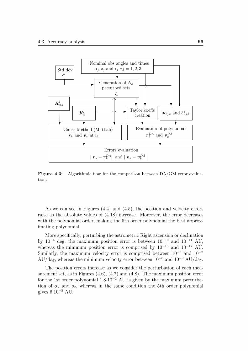
4.3. Accuracy analysis 66
Nominal obs angles and timesαj, δj and tj ∀j = 1, 2, 3
Rj⊕
Rjobs
Gauss Method (MatLab)r k and v k at t2
Generation of Ns
Ik
Std devσ
δαj,k and δδj,k
Evaluation of polynomials
rDAk and vDA
k
perturbed sets
Taylor coeffscreation
Errors evaluation
||r k − rDAk || and ||v k − vDA
k ||
Figure 4.3: Algorithmic flow for the comparison between DA/GM error evalua-tion.
As we can see in Figures (4.4) and (4.5), the position and velocity errorsraise as the absolute values of (4.18) increase. Moreover, the error decreaseswith the polynomial order, making the 5th order polynomial the best approx-imating polynomial.
More specifically, perturbing the astrometric Right ascension or declinationby 10−4 deg, the maximum position error is between 10−10 and 10−11 AU,whereas the minimum position error is comprised by 10−16 and 10−17 AU.Similarly, the maximum velocity error is comprised between 10−3 and 10−2
AU/day, whereas the minimum velocity error between 10−8 and 10−9 AU/day.
The position errors increase as we consider the perturbation of each mea-surement set, as in Figures (4.6), (4.7) and (4.8). The maximum position errorfor the 1st order polynomial 1.8·10−2 AU is given by the maximum perturba-tion of α2 and δ2, whereas in the same condition the 5th order polynomialgives 6·10−5 AU.
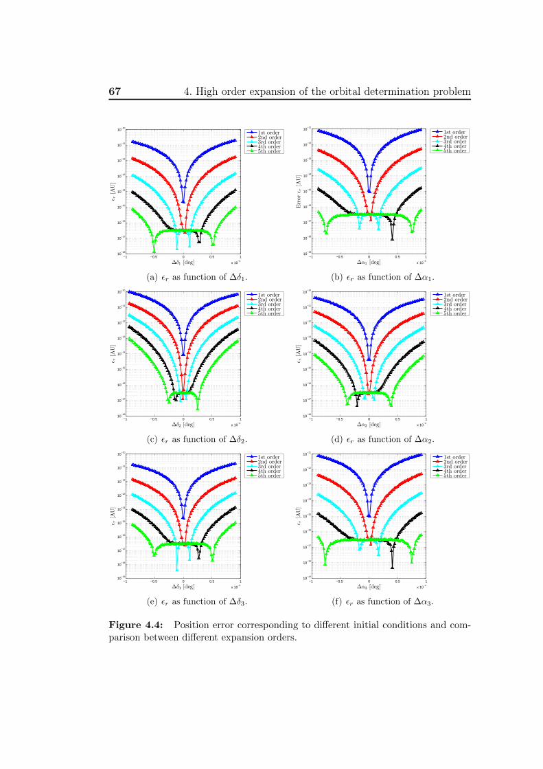
67 4. High order expansion of the orbital determination problem
−1 −0.5 0 0.5 1
x 10−4
10−18
10−17
10−16
10−15
10−14
10−13
10−12
10−11
10−10
Δδ1 [deg]
ε r[A
U]
1st order2nd order3rd order4th order5th order
(a) εr as function of ∆δ1.
−1 −0.5 0 0.5 1
x 10−4
10−19
10−18
10−17
10−16
10−15
10−14
10−13
10−12
10−11
Δα1 [deg]
Err
or
ε r[A
U]
1st order2nd order3rd order4th order5th order
(b) εr as function of ∆α1.
−1 −0.5 0 0.5 1
x 10−4
10−18
10−17
10−16
10−15
10−14
10−13
10−12
10−11
10−10
Δδ2 [deg]
ε r[A
U]
1st order2nd order3rd order4th order5th order
(c) εr as function of ∆δ2.
−1 −0.5 0 0.5 1
x 10−4
10−18
10−17
10−16
10−15
10−14
10−13
10−12
10−11
10−10
Δα2 [deg]
ε r[A
U]
1st order2nd order3rd order4th order5th order
(d) εr as function of ∆α2.
−1 −0.5 0 0.5 1
x 10−4
10−19
10−18
10−17
10−16
10−15
10−14
10−13
10−12
10−11
10−10
Δδ3 [deg]
ε r[A
U]
1st order2nd order3rd order4th order5th order
(e) εr as function of ∆δ3.
−1 −0.5 0 0.5 1
x 10−4
10−19
10−18
10−17
10−16
10−15
10−14
10−13
10−12
10−11
Δα3 [deg]
ε r[A
U]
1st order2nd order3rd order4th order5th order
(f) εr as function of ∆α3.
Figure 4.4: Position error corresponding to different initial conditions and com-parison between different expansion orders.
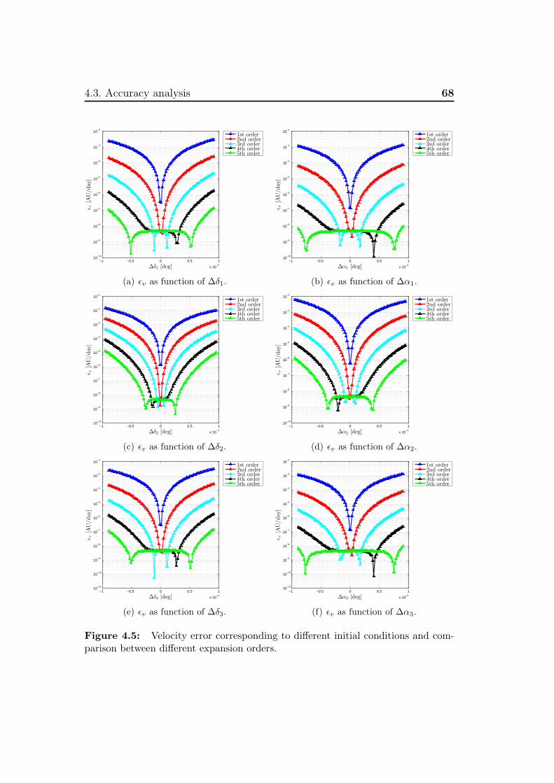
4.3. Accuracy analysis 68
−1 −0.5 0 0.5 1
x 10−4
10−10
10−9
10−8
10−7
10−6
10−5
10−4
10−3
10−2
Δδ1 [deg]
ε v[A
U/day
]
1st order2nd order3rd order4th order5th order
(a) εv as function of ∆δ1.
−1 −0.5 0 0.5 1
x 10−4
10−10
10−9
10−8
10−7
10−6
10−5
10−4
10−3
10−2
Δα1 [deg]
ε v[A
U/day
]
1st order2nd order3rd order4th order5th order
(b) εv as function of ∆α1.
−1 −0.5 0 0.5 1
x 10−4
10−10
10−9
10−8
10−7
10−6
10−5
10−4
10−3
10−2
10−1
Δδ2 [deg]
ε v[A
U/day
]
1st order2nd order3rd order4th order5th order
(c) εv as function of ∆δ2.
−1 −0.5 0 0.5 1
x 10−4
10−10
10−9
10−8
10−7
10−6
10−5
10−4
10−3
10−2
Δα2 [deg]
ε v[A
U/day
]
1st order2nd order3rd order4th order5th order
(d) εv as function of ∆α2.
−1 −0.5 0 0.5 1
x 10−4
10−11
10−10
10−9
10−8
10−7
10−6
10−5
10−4
10−3
10−2
Δδ3 [deg]
ε v[A
U/day
]
1st order2nd order3rd order4th order5th order
(e) εv as function of ∆δ3.
−1 −0.5 0 0.5 1
x 10−4
10−11
10−10
10−9
10−8
10−7
10−6
10−5
10−4
10−3
10−2
Δα3 [deg]
ε v[A
U/day
]
1st order2nd order3rd order4th order5th order
(f) εv as function of ∆α3.
Figure 4.5: Velocity error corresponding to different initial conditions and com-parison between different expansion orders.
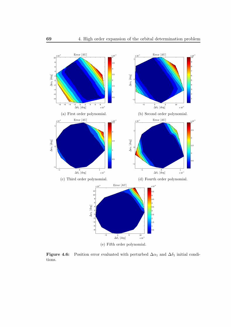
69 4. High order expansion of the orbital determination problem
Δδ1 [deg]
Δα
1[d
eg]
Error [AU]
−8 −6 −4 −2 0 2 4 6 8
x 10−5
−8
−6
−4
−2
0
2
4
6
8
10x 10
−5
0.5
1
1.5
2
2.5
3
3.5
4x 10
−3
(a) First order polynomial.
Δδ1 [deg]
Δα
1[d
eg]
Error [AU]
−5 0 5 10
x 10−5
−1
0
1
x 10−4
1
2
3
4
5
6
7
8
9
10x 10
−4
(b) Second order polynomial.
Δδ1 [deg]
Δα
1[d
eg]
Error [AU]
−1 0 1
x 10−4
−1
0
1
x 10−4
0.5
1
1.5
2
2.5x 10
−4
(c) Third order polynomial.
Δδ1 [deg]
Δα
1[d
eg]
Error [AU]
−1 0 1
x 10−4
−1
0
1
x 10−4
0.5
1
1.5
2
2.5
3x 10
−5
(d) Fourth order polynomial.
Δδ1 [deg]
Δα
1[d
eg]
Error [AU]
−5 0 5 10
x 10−5
−8
−6
−4
−2
0
2
4
6
8
10
12
x 10−5
0.5
1
1.5
2
2.5
3
3.5
4
4.5
5
5.5
x 10−6
(e) Fifth order polynomial.
Figure 4.6: Position error evaluated with perturbed ∆α1 and ∆δ1 initial condi-tions.
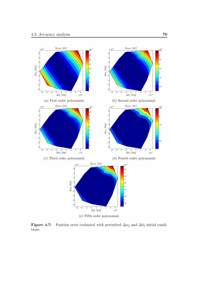
4.3. Accuracy analysis 70
Δδ2 [deg]
Δα
2[d
eg]
Error [AU]
−8 −6 −4 −2 0 2 4 6 8
x 10−5
−8
−6
−4
−2
0
2
4
6
8
x 10−5
2
4
6
8
10
12
14
16
18x 10
−3
(a) First order polynomial.
Δδ2 [deg]
Δα
2[d
eg]
Error [AU]
−8 −6 −4 −2 0 2 4 6 8
x 10−5
−8
−6
−4
−2
0
2
4
6
8
x 10−5
0.5
1
1.5
2
2.5
3
3.5
4
4.5x 10
−3
(b) Second order polynomial.
Δδ2 [deg]
Δα
2[d
eg]
Error [AU]
−8 −6 −4 −2 0 2 4 6 8
x 10−5
−8
−6
−4
−2
0
2
4
6
8
x 10−5
1
2
3
4
5
6
7
8
9
10
11x 10
−4
(c) Third order polynomial.
Δδ2 [deg]
Δα
2[d
eg]
Error [AU]
−8 −6 −4 −2 0 2 4 6 8
x 10−5
−8
−6
−4
−2
0
2
4
6
8
x 10−5
0.5
1
1.5
2
2.5x 10
−4
(d) Fourth order polynomial.
Δδ2 [deg]
Δα
2[d
eg]
Error [AU]
−8 −6 −4 −2 0 2 4 6 8
x 10−5
−8
−6
−4
−2
0
2
4
6
8
x 10−5
0.5
1
1.5
2
2.5
3
3.5
4
4.5
5
5.5
6x 10
−5
(e) Fifth order polynomial.
Figure 4.7: Position error evaluated with perturbed ∆α2 and ∆δ2 initial condi-tions.
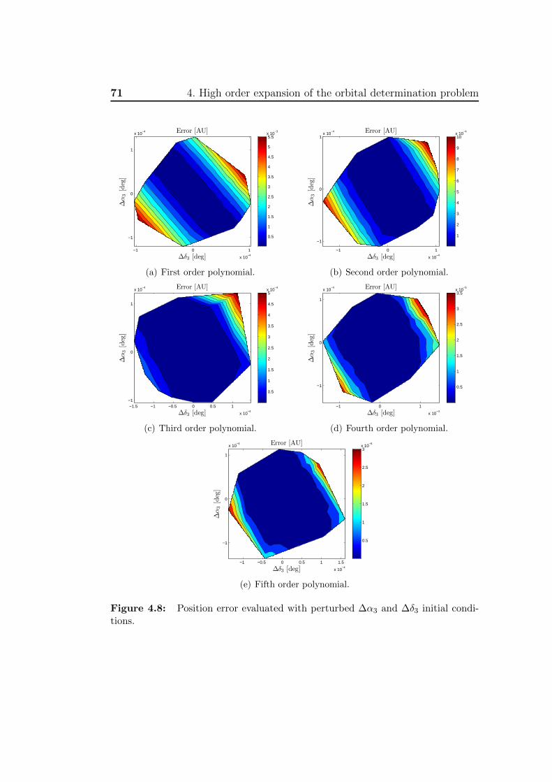
71 4. High order expansion of the orbital determination problem
Δδ3 [deg]
Δα
3[d
eg]
Error [AU]
−1 0 1
x 10−4
−1
0
1
x 10−4
0.5
1
1.5
2
2.5
3
3.5
4
4.5
5
5.5x 10
−3
(a) First order polynomial.
Δδ3 [deg]
Δα
3[d
eg]
Error [AU]
−1 0 1
x 10−4
−1
0
1x 10
−4
1
2
3
4
5
6
7
8
9
10x 10
−4
(b) Second order polynomial.
Δδ3 [deg]
Δα
3[d
eg]
Error [AU]
−1.5 −1 −0.5 0 0.5 1
x 10−4
−1
0
1
x 10−4
0.5
1
1.5
2
2.5
3
3.5
4
4.5
5x 10
−4
(c) Third order polynomial.
Δδ3 [deg]
Δα
3[d
eg]
Error [AU]
−1 0 1
x 10−4
−1
0
1
x 10−4
0.5
1
1.5
2
2.5
3
3.5x 10
−5
(d) Fourth order polynomial.
Δδ3 [deg]
Δα
3[d
eg]
Error [AU]
−1 −0.5 0 0.5 1 1.5
x 10−4
−1
0
1
x 10−4
0.5
1
1.5
2
2.5
3x 10
−6
(e) Fifth order polynomial.
Figure 4.8: Position error evaluated with perturbed ∆α3 and ∆δ3 initial condi-tions.
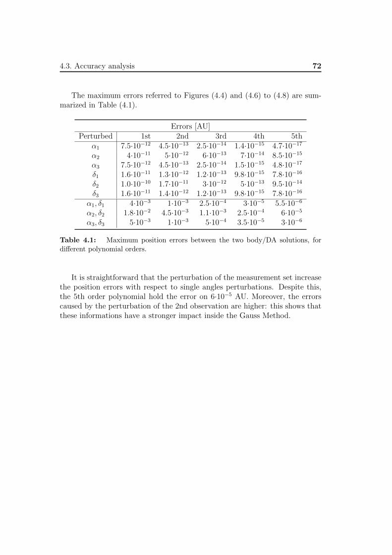
4.3. Accuracy analysis 72
The maximum errors referred to Figures (4.4) and (4.6) to (4.8) are sum-marized in Table (4.1).
Errors [AU]Perturbed 1st 2nd 3rd 4th 5th
α1 7.5·10−12 4.5·10−13 2.5·10−14 1.4·10−15 4.7·10−17
α2 4·10−11 5·10−12 6·10−13 7·10−14 8.5·10−15
α3 7.5·10−12 4.5·10−13 2.5·10−14 1.5·10−15 4.8·10−17
δ1 1.6·10−11 1.3·10−12 1.2·10−13 9.8·10−15 7.8·10−16
δ2 1.0·10−10 1.7·10−11 3·10−12 5·10−13 9.5·10−14
δ3 1.6·10−11 1.4·10−12 1.2·10−13 9.8·10−15 7.8·10−16
α1, δ1 4·10−3 1·10−3 2.5·10−4 3·10−5 5.5·10−6
α2, δ2 1.8·10−2 4.5·10−3 1.1·10−3 2.5·10−4 6·10−5
α3, δ3 5·10−3 1·10−3 5·10−4 3.5·10−5 3·10−6
Table 4.1: Maximum position errors between the two body/DA solutions, fordifferent polynomial orders.
It is straightforward that the perturbation of the measurement set increasethe position errors with respect to single angles perturbations. Despite this,the 5th order polynomial hold the error on 6·10−5 AU. Moreover, the errorscaused by the perturbation of the 2nd observation are higher: this shows thatthese informations have a stronger impact inside the Gauss Method.
Chapter 5
High order Mapping of VirtualAsteroids
The aim of this chapter is to show how the uncertainties associated to theorbit determination process can be mapped forward in time using DifferentialAlgebra. As a result, Virtual Asteroids are computed at a generic epoch t4.Moreover, an intensive analysis over the polynomial order providing the leasterrors between the two approaches will be presented.
In order to perform a close-loop analysis of the problem, simulated ob-servations of real asteroids are considered. The orbital ephemerides of theseasteroids are taken from Minor Planets Center. These ephemerides have beenused to compute the topocentric astrometric angles (αi, δi) ∀i = 1, 2, 3 makingthe problem well posed. This choice has the advantage to provide a referencevalue of COEs, thus avoiding the calculation of false/unaccurate GM solutionsand thus unaccurate DA polynomials.
In order to simulate the evolution of the VAs clouds in time, six simulationsat different epochs are considered. The vector of epochs is
T4 = 0.5, 1, 2, 5, 10, 20 days after t2 , (5.1)
being t2 the central observation time of GM solution.
5.1 Virtual Asteroids mapping
The ultimate goal of this thesis work is the calculation of the regions of thecelestial sphere (α, δ) to be observed in order to track a newly discoveredobject. This region is obtained by propagating the so-called Virtual Asteroids,through the evaluation of the Taylor polynomials αDA, δDA at an epoch t4 > t3.
73
5.1. Virtual Asteroids mapping 74
The high order maps are obtained by expanding the flow of the ODE ofthe two-body problem as detailed in [5]. The vectors rDA and vDA at t2 areused as initial conditions of the COSY INFINITY routine [5], which computesthe Taylor polynomials of the state vectors rDAt4 and vDAt4 at any epoch t4 of(5.1).
Then, the polynomials of the heliocentric position vectors rDAt4 are used tocompute the cosine vector polynomials ρt4 of the asteroid at t4, by subtractingthe Earth ephemeris vector Rt4
⊕ and the observer position vector Rt4obs at same
epoch:
ρt4ρDAt4 = rDAt4 −Rt4
⊕ −Rt4obs . (5.2)
The Taylor polynomials of the astrometric angles at t4 are then computedas
δDA = arcsin ρDAz,t4
αDA =arccos ρDAx,t4
cos δDAt4,
(5.3)
being
ρDAt4 = ρDAx,t4 , ρDAy,t4 , ρDAz,t4T . (5.4)
Considering a typical Gaussian probability distribution about the nominalangles, with a conservative value of the standard deviation σ =1.5 10−1 arcsec[7], Ns sets Ik of randomly created astrometric angles have been generated;i.e.
Ik = α1,k, α2,k, α3,k, δ1,k, δ2,k, δ3,k k = 1, ..., Ns . (5.5)
Then, the astrometric angles’ polynomials αDA and δDA at t4 are evaluatedat
δαj,k = αj,k − α0j and δδj,k = δj,k − δ0j , (5.6)
identifying the Ns Virtual Asteroids astrometric pair αk, δk at t4. Thealgorithm for VAs polynomials creation and evaluation is presented in Figure(5.1).
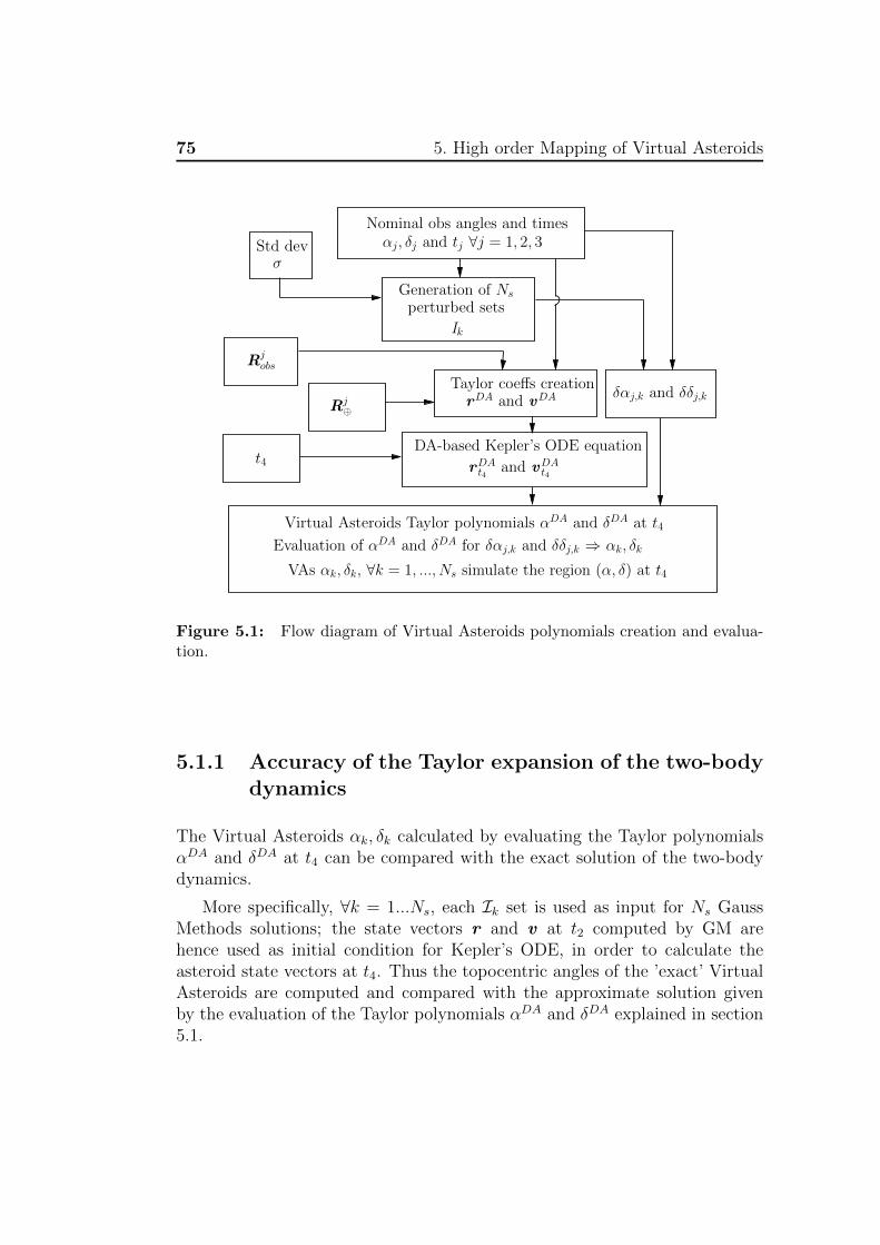
75 5. High order Mapping of Virtual Asteroids
Nominal obs angles and timesαj, δj and tj ∀j = 1, 2, 3
Rj⊕
Rjobs
Generation of Ns
Ik
Std devσ
δαj,k and δδj,k
perturbed sets
Taylor coeffs creationrDA and vDA
DA-based Kepler’s ODE equationt4 rDA
t4and vDA
t4
Virtual Asteroids Taylor polynomials αDA and δDA at t4
Evaluation of αDA and δDA for δαj,k and δδj,k ⇒ αk, δk
VAs αk, δk, ∀k = 1, ..., Ns simulate the region (α, δ) at t4
Figure 5.1: Flow diagram of Virtual Asteroids polynomials creation and evalua-tion.
5.1.1 Accuracy of the Taylor expansion of the two-bodydynamics
The Virtual Asteroids αk, δk calculated by evaluating the Taylor polynomialsαDA and δDA at t4 can be compared with the exact solution of the two-bodydynamics.
More specifically, ∀k = 1...Ns, each Ik set is used as input for Ns GaussMethods solutions; the state vectors r and v at t2 computed by GM arehence used as initial condition for Kepler’s ODE, in order to calculate theasteroid state vectors at t4. Thus the topocentric angles of the ’exact’ VirtualAsteroids are computed and compared with the approximate solution givenby the evaluation of the Taylor polynomials αDA and δDA explained in section5.1.
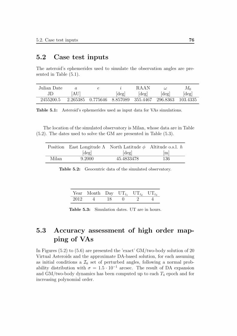
5.2. Case test inputs 76
5.2 Case test inputs
The asteroid’s ephemerides used to simulate the observation angles are pre-sented in Table (5.1).
Julian Date a e i RAAN ω M0
JD [AU] [deg] [deg] [deg] [deg]2455200.5 2.265385 0.775646 8.857089 355.4467 296.8363 103.4335
Table 5.1: Asteroid’s ephemerides used as input data for VAs simulations.
The location of the simulated observatory is Milan, whose data are in Table(5.2). The dates used to solve the GM are presented in Table (5.3).
Position East Longitude Λ North Latitude φ Altitude o.s.l. h[deg] [deg] [m]
Milan 9.2000 45.4833478 136
Table 5.2: Geocentric data of the simulated observatory.
Year Month Day UTt1 UTt2 UTt3
2012 4 18 0 2 4
Table 5.3: Simulation dates. UT are in hours.
5.3 Accuracy assessment of high order map-
ping of VAs
In Figures (5.2) to (5.6) are presented the ’exact’ GM/two-body solution of 20Virtual Asteroids and the approximate DA-based solution, for each assumingas initial conditions a Ik set of perturbed angles, following a normal prob-ability distribution with σ = 1.5 · 10−1 arcsec. The result of DA expansionand GM/two-body dynamics has been computed up to each T4 epoch and forincreasing polynomial order.
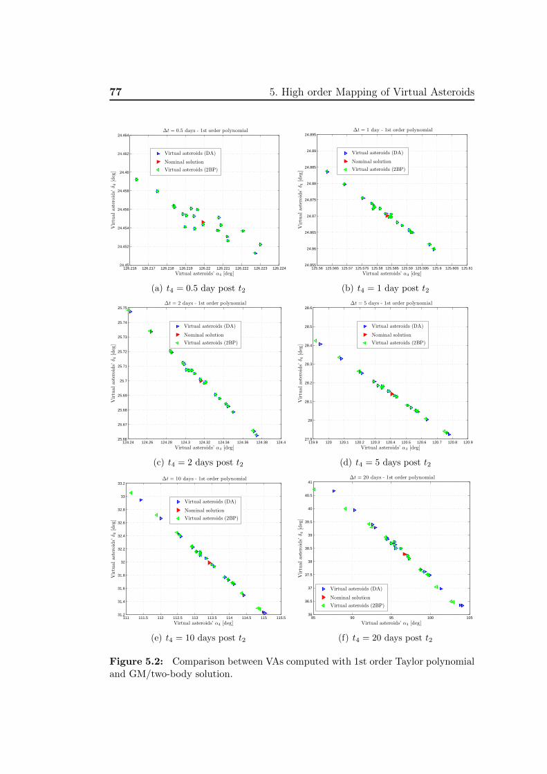
77 5. High order Mapping of Virtual Asteroids
126.216 126.217 126.218 126.219 126.22 126.221 126.222 126.223 126.22424.45
24.452
24.454
24.456
24.458
24.46
24.462
24.464
Virtual asteroids’ α4 [deg]
Virtu
alast
eroid
s’δ 4
[deg
]
Δt = 0.5 days - 1st order polynomial
Virtual asteroids (DA)
Nominal solution
Virtual asteroids (2BP)
(a) t4 = 0.5 day post t2
125.56 125.565 125.57 125.575 125.58 125.585 125.59 125.595 125.6 125.605 125.6124.855
24.86
24.865
24.87
24.875
24.88
24.885
24.89
24.895
Virtual asteroids’ α4 [deg]
Virtu
alast
eroid
s’δ 4
[deg
]
Δt = 1 day - 1st order polynomial
Virtual asteroids (DA)
Nominal solution
Virtual asteroids (2BP)
(b) t4 = 1 day post t2
124.24 124.26 124.28 124.3 124.32 124.34 124.36 124.38 124.425.66
25.67
25.68
25.69
25.7
25.71
25.72
25.73
25.74
25.75
Virtual asteroids’ α4 [deg]
Virtu
alast
eroid
s’δ 4
[deg
]
Δt = 2 days - 1st order polynomial
Virtual asteroids (DA)
Nominal solution
Virtual asteroids (2BP)
(c) t4 = 2 days post t2
119.9 120 120.1 120.2 120.3 120.4 120.5 120.6 120.7 120.8 120.927.9
28
28.1
28.2
28.3
28.4
28.5
28.6
Virtual asteroids’ α4 [deg]
Virtu
alast
eroid
s’δ 4
[deg
]Δt = 5 days - 1st order polynomial
Virtual asteroids (DA)
Nominal solution
Virtual asteroids (2BP)
(d) t4 = 5 days post t2
111 111.5 112 112.5 113 113.5 114 114.5 115 115.531.2
31.4
31.6
31.8
32
32.2
32.4
32.6
32.8
33
33.2
Virtual asteroids’ α4 [deg]
Virtu
alast
eroid
s’δ 4
[deg
]
Δt = 10 days - 1st order polynomial
Virtual asteroids (DA)
Nominal solution
Virtual asteroids (2BP)
(e) t4 = 10 days post t2
85 90 95 100 10536
36.5
37
37.5
38
38.5
39
39.5
40
40.5
41
Virtual asteroids’ α4 [deg]
Virtu
alast
eroid
s’δ 4
[deg
]
Δt = 20 days - 1st order polynomial
Virtual asteroids (DA)
Nominal solution
Virtual asteroids (2BP)
(f) t4 = 20 days post t2
Figure 5.2: Comparison between VAs computed with 1st order Taylor polynomialand GM/two-body solution.
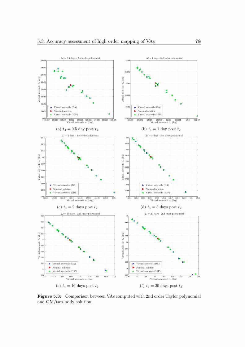
5.3. Accuracy assessment of high order mapping of VAs 78
126.217 126.218 126.219 126.22 126.221 126.222 126.223 126.224 126.22524.45
24.451
24.452
24.453
24.454
24.455
24.456
24.457
24.458
Virtual asteroids’ α4 [deg]
Virtu
alast
eroid
s’δ 4
[deg
]
Δt = 0.5 days - 2nd order polynomial
Virtual asteroids (DA)
Nominal solution
Virtual asteroids (2BP)
(a) t4 = 0.5 day post t2
125.57 125.575 125.58 125.585 125.59 125.595 125.6 125.60524.855
24.86
24.865
24.87
24.875
24.88
Virtual asteroids’ α4 [deg]V
irtu
alast
eroid
s’δ 4
[deg
]
Δt = 1 day - 2nd order polynomial
Virtual asteroids (DA)
Nominal solution
Virtual asteroids (2BP)
(b) t4 = 1 day post t2
124.24 124.26 124.28 124.3 124.32 124.34 124.36 124.38 124.425.64
25.65
25.66
25.67
25.68
25.69
25.7
25.71
25.72
25.73
Virtual asteroids’ α4 [deg]
Virtu
alast
eroid
s’δ 4
[deg
]
Δt = 2 days - 2nd order polynomial
Virtual asteroids (DA)
Nominal solution
Virtual asteroids (2BP)
(c) t4 = 2 days post t2
120.1 120.2 120.3 120.4 120.5 120.6 120.7 120.8 120.9 121 121.127.8
27.85
27.9
27.95
28
28.05
28.1
28.15
28.2
28.25
28.3
Virtual asteroids’ α4 [deg]
Virtu
alast
eroid
s’δ 4
[deg
]
Δt = 5 days - 2nd order polynomial
Virtual asteroids (DA)
Nominal solution
Virtual asteroids (2BP)
(d) t4 = 5 days post t2
112 112.5 113 113.5 114 114.5 115 115.5 11630.8
31
31.2
31.4
31.6
31.8
32
32.2
32.4
32.6
32.8
Virtual asteroids’ α4 [deg]
Virtu
alast
eroid
s’δ 4
[deg
]
Δt = 10 days - 2nd order polynomial
Virtual asteroids (DA)
Nominal solution
Virtual asteroids (2BP)
(e) t4 = 10 days post t2
90 92 94 96 98 100 102 104 10635.5
36
36.5
37
37.5
38
38.5
39
39.5
40
Virtual asteroids’ α4 [deg]
Virtu
alast
eroid
s’δ 4
[deg
]
Δt = 20 days - 2nd order polynomial
Virtual asteroids (DA)
Nominal solution
Virtual asteroids (2BP)
(f) t4 = 20 days post t2
Figure 5.3: Comparison between VAs computed with 2nd order Taylor polynomialand GM/two-body solution.

79 5. High order Mapping of Virtual Asteroids
126.216 126.217 126.218 126.219 126.22 126.221 126.222 126.223 126.22424.45
24.452
24.454
24.456
24.458
24.46
24.462
24.464
Virtual asteroids’ α4 [deg]
Virtu
alast
eroid
s’δ 4
[deg
]
Δt = 0.5 days - 3rd order polynomial
Virtual asteroids (DA)
Nominal solution
Virtual asteroids (2BP)
(a) t4 = 0.5 day post t2
125.56 125.565 125.57 125.575 125.58 125.585 125.59 125.595 125.6 125.605 125.6124.855
24.86
24.865
24.87
24.875
24.88
24.885
24.89
24.895
Virtual asteroids’ α4 [deg]
Virtu
alast
eroid
s’δ 4
[deg
]
Δt = 1 day - 3rd order polynomial
Virtual asteroids (DA)
Nominal solution
Virtual asteroids (2BP)
(b) t4 = 1 day post t2
124.24 124.26 124.28 124.3 124.32 124.34 124.36 124.38 124.425.66
25.67
25.68
25.69
25.7
25.71
25.72
25.73
25.74
25.75
Virtual asteroids’ α4 [deg]
Virtu
alast
eroid
s’δ 4
[deg
]
Δt = 2 days - 3rd order polynomial
Virtual asteroids (DA)
Nominal solution
Virtual asteroids (2BP)
(c) t4 = 2 days post t2
119.9 120 120.1 120.2 120.3 120.4 120.5 120.6 120.7 120.8 120.927.9
28
28.1
28.2
28.3
28.4
28.5
28.6
Virtual asteroids’ α4 [deg]
Virtu
alast
eroid
s’δ 4
[deg
]Δt = 5 days - 3rd order polynomial
Virtual asteroids (DA)
Nominal solution
Virtual asteroids (2BP)
(d) t4 = 5 days post t2
111 111.5 112 112.5 113 113.5 114 114.5 11531.2
31.4
31.6
31.8
32
32.2
32.4
32.6
32.8
33
33.2
Virtual asteroids’ α4 [deg]
Virtu
alast
eroid
s’δ 4
[deg
]
Δt = 10 days - 3rd order polynomial
Virtual asteroids (DA)
Nominal solution
Virtual asteroids (2BP)
(e) t4 = 10 days post t2
84 86 88 90 92 94 96 98 100 102 10436
36.5
37
37.5
38
38.5
39
39.5
40
40.5
41
Virtual asteroids’ α4 [deg]
Virtu
alast
eroid
s’δ 4
[deg
]
Δt = 20 days - 3rd order polynomial
Virtual asteroids (DA)
Nominal solution
Virtual asteroids (2BP)
(f) t4 = 20 days post t2
Figure 5.4: Comparison between VAs computed with 3rd order Taylor polynomialand GM/two-body solution.
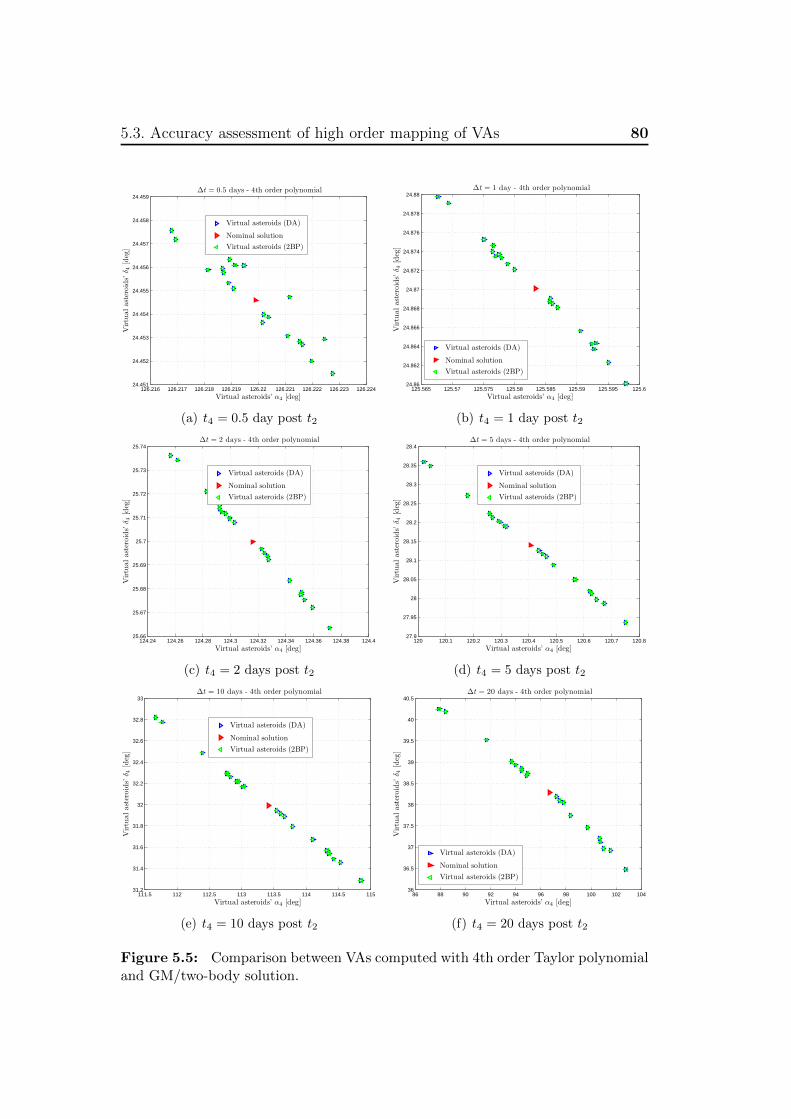
5.3. Accuracy assessment of high order mapping of VAs 80
126.216 126.217 126.218 126.219 126.22 126.221 126.222 126.223 126.22424.451
24.452
24.453
24.454
24.455
24.456
24.457
24.458
24.459
Virtual asteroids’ α4 [deg]
Virtu
alast
eroid
s’δ 4
[deg
]
Δt = 0.5 days - 4th order polynomial
Virtual asteroids (DA)
Nominal solution
Virtual asteroids (2BP)
(a) t4 = 0.5 day post t2
125.565 125.57 125.575 125.58 125.585 125.59 125.595 125.624.86
24.862
24.864
24.866
24.868
24.87
24.872
24.874
24.876
24.878
24.88
Virtual asteroids’ α4 [deg]V
irtu
alast
eroid
s’δ 4
[deg
]
Δt = 1 day - 4th order polynomial
Virtual asteroids (DA)
Nominal solution
Virtual asteroids (2BP)
(b) t4 = 1 day post t2
124.24 124.26 124.28 124.3 124.32 124.34 124.36 124.38 124.425.66
25.67
25.68
25.69
25.7
25.71
25.72
25.73
25.74
Virtual asteroids’ α4 [deg]
Virtu
alast
eroid
s’δ 4
[deg
]
Δt = 2 days - 4th order polynomial
Virtual asteroids (DA)
Nominal solution
Virtual asteroids (2BP)
(c) t4 = 2 days post t2
120 120.1 120.2 120.3 120.4 120.5 120.6 120.7 120.827.9
27.95
28
28.05
28.1
28.15
28.2
28.25
28.3
28.35
28.4
Virtual asteroids’ α4 [deg]
Virtu
alast
eroid
s’δ 4
[deg
]
Δt = 5 days - 4th order polynomial
Virtual asteroids (DA)
Nominal solution
Virtual asteroids (2BP)
(d) t4 = 5 days post t2
111.5 112 112.5 113 113.5 114 114.5 11531.2
31.4
31.6
31.8
32
32.2
32.4
32.6
32.8
33
Virtual asteroids’ α4 [deg]
Virtu
alast
eroid
s’δ 4
[deg
]
Δt = 10 days - 4th order polynomial
Virtual asteroids (DA)
Nominal solution
Virtual asteroids (2BP)
(e) t4 = 10 days post t2
86 88 90 92 94 96 98 100 102 10436
36.5
37
37.5
38
38.5
39
39.5
40
40.5
Virtual asteroids’ α4 [deg]
Virtu
alast
eroid
s’δ 4
[deg
]
Δt = 20 days - 4th order polynomial
Virtual asteroids (DA)
Nominal solution
Virtual asteroids (2BP)
(f) t4 = 20 days post t2
Figure 5.5: Comparison between VAs computed with 4th order Taylor polynomialand GM/two-body solution.
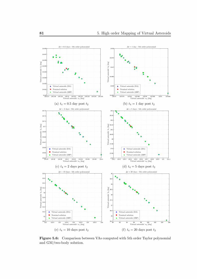
81 5. High order Mapping of Virtual Asteroids
126.217 126.218 126.219 126.22 126.221 126.222 126.223 126.224 126.22524.45
24.451
24.452
24.453
24.454
24.455
24.456
24.457
24.458
Virtual asteroids’ α4 [deg]
Virtu
alast
eroid
s’δ 4
[deg
]
Δt = 0.5 days - 5th order polynomial
Virtual asteroids (DA)
Nominal solution
Virtual asteroids (2BP)
(a) t4 = 0.5 day post t2
125.57 125.575 125.58 125.585 125.59 125.595 125.6 125.60524.855
24.86
24.865
24.87
24.875
24.88
Virtual asteroids’ α4 [deg]
Virtu
alast
eroid
s’δ 4
[deg
]
Δt = 1 day - 5th order polynomial
Virtual asteroids (DA)
Nominal solution
Virtual asteroids (2BP)
(b) t4 = 1 day post t2
124.24 124.26 124.28 124.3 124.32 124.34 124.36 124.38 124.425.64
25.65
25.66
25.67
25.68
25.69
25.7
25.71
25.72
25.73
Virtual asteroids’ α4 [deg]
Virtu
alast
eroid
s’δ 4
[deg
]
Δt = 2 days - 5th order polynomial
Virtual asteroids (DA)
Nominal solution
Virtual asteroids (2BP)
(c) t4 = 2 days post t2
120.1 120.2 120.3 120.4 120.5 120.6 120.7 120.8 120.9 121 121.127.8
27.85
27.9
27.95
28
28.05
28.1
28.15
28.2
28.25
28.3
Virtual asteroids’ α4 [deg]
Virtu
alast
eroid
s’δ 4
[deg
]Δt = 5 days - 5th order polynomial
Virtual asteroids (DA)
Nominal solution
Virtual asteroids (2BP)
(d) t4 = 5 days post t2
112 112.5 113 113.5 114 114.5 115 115.5 11630.8
31
31.2
31.4
31.6
31.8
32
32.2
32.4
32.6
32.8
Virtual asteroids’ α4 [deg]
Virtu
alast
eroid
s’δ 4
[deg
]
Δt = 10 days - 5th order polynomial
Virtual asteroids (DA)
Nominal solution
Virtual asteroids (2BP)
(e) t4 = 10 days post t2
90 92 94 96 98 100 102 104 10635.5
36
36.5
37
37.5
38
38.5
39
39.5
40
Virtual asteroids’ α4 [deg]
Virtu
alast
eroid
s’δ 4
[deg
]
Δt = 20 days - 5th order polynomial
Virtual asteroids (DA)
Nominal solution
Virtual asteroids (2BP)
(f) t4 = 20 days post t2
Figure 5.6: Comparison between VAs computed with 5th order Taylor polynomialand GM/two-body solution.
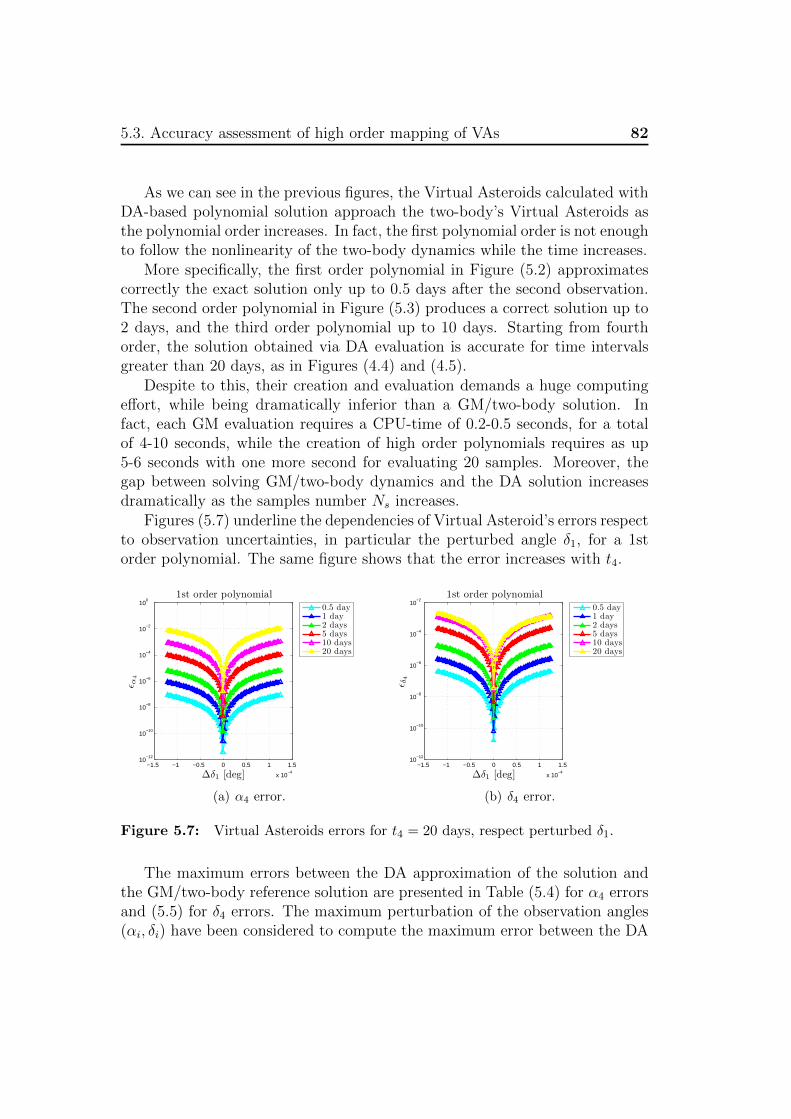
5.3. Accuracy assessment of high order mapping of VAs 82
As we can see in the previous figures, the Virtual Asteroids calculated withDA-based polynomial solution approach the two-body’s Virtual Asteroids asthe polynomial order increases. In fact, the first polynomial order is not enoughto follow the nonlinearity of the two-body dynamics while the time increases.
More specifically, the first order polynomial in Figure (5.2) approximatescorrectly the exact solution only up to 0.5 days after the second observation.The second order polynomial in Figure (5.3) produces a correct solution up to2 days, and the third order polynomial up to 10 days. Starting from fourthorder, the solution obtained via DA evaluation is accurate for time intervalsgreater than 20 days, as in Figures (4.4) and (4.5).
Despite to this, their creation and evaluation demands a huge computingeffort, while being dramatically inferior than a GM/two-body solution. Infact, each GM evaluation requires a CPU-time of 0.2-0.5 seconds, for a totalof 4-10 seconds, while the creation of high order polynomials requires as up5-6 seconds with one more second for evaluating 20 samples. Moreover, thegap between solving GM/two-body dynamics and the DA solution increasesdramatically as the samples number Ns increases.
Figures (5.7) underline the dependencies of Virtual Asteroid’s errors respectto observation uncertainties, in particular the perturbed angle δ1, for a 1storder polynomial. The same figure shows that the error increases with t4.
−1.5 −1 −0.5 0 0.5 1 1.5
x 10−4
10−12
10−10
10−8
10−6
10−4
10−2
100
Δδ1 [deg]
ε α4
1st order polynomial
0.5 day1 day2 days5 days10 days20 days
(a) α4 error.
−1.5 −1 −0.5 0 0.5 1 1.5
x 10−4
10−12
10−10
10−8
10−6
10−4
10−2
Δδ1 [deg]
ε δ4
1st order polynomial
0.5 day1 day2 days5 days10 days20 days
(b) δ4 error.
Figure 5.7: Virtual Asteroids errors for t4 = 20 days, respect perturbed δ1.
The maximum errors between the DA approximation of the solution andthe GM/two-body reference solution are presented in Table (5.4) for α4 errorsand (5.5) for δ4 errors. The maximum perturbation of the observation angles(αi, δi) have been considered to compute the maximum error between the DA
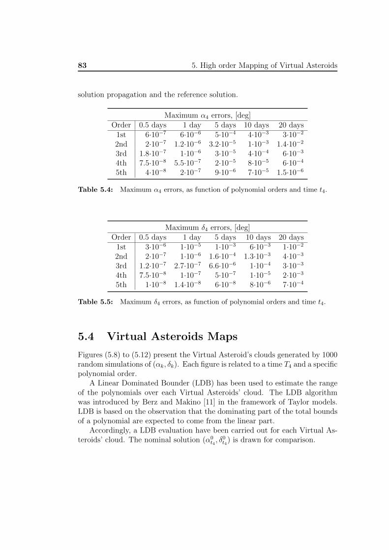
83 5. High order Mapping of Virtual Asteroids
solution propagation and the reference solution.
Maximum α4 errors, [deg]Order 0.5 days 1 day 5 days 10 days 20 days
1st 6·10−7 6·10−6 5·10−4 4·10−3 3·10−2
2nd 2·10−7 1.2·10−6 3.2·10−5 1·10−3 1.4·10−2
3rd 1.8·10−7 1·10−6 3·10−5 4·10−4 6·10−3
4th 7.5·10−8 5.5·10−7 2·10−5 8·10−5 6·10−4
5th 4·10−8 2·10−7 9·10−6 7·10−5 1.5·10−6
Table 5.4: Maximum α4 errors, as function of polynomial orders and time t4.
Maximum δ4 errors, [deg]Order 0.5 days 1 day 5 days 10 days 20 days
1st 3·10−6 1·10−5 1·10−3 6·10−3 1·10−2
2nd 2·10−7 1·10−6 1.6·10−4 1.3·10−3 4·10−3
3rd 1.2·10−7 2.7·10−7 6.6·10−6 1·10−4 3·10−3
4th 7.5·10−8 1·10−7 5·10−7 1·10−5 2·10−3
5th 1·10−8 1.4·10−8 6·10−8 8·10−6 7·10−4
Table 5.5: Maximum δ4 errors, as function of polynomial orders and time t4.
5.4 Virtual Asteroids Maps
Figures (5.8) to (5.12) present the Virtual Asteroid’s clouds generated by 1000random simulations of (αk, δk). Each figure is related to a time T4 and a specificpolynomial order.
A Linear Dominated Bounder (LDB) has been used to estimate the rangeof the polynomials over each Virtual Asteroids’ cloud. The LDB algorithmwas introduced by Berz and Makino [11] in the framework of Taylor models.LDB is based on the observation that the dominating part of the total boundsof a polynomial are expected to come from the linear part.
Accordingly, a LDB evaluation have been carried out for each Virtual As-teroids’ cloud. The nominal solution (α0
t4, δ0t4) is drawn for comparison.
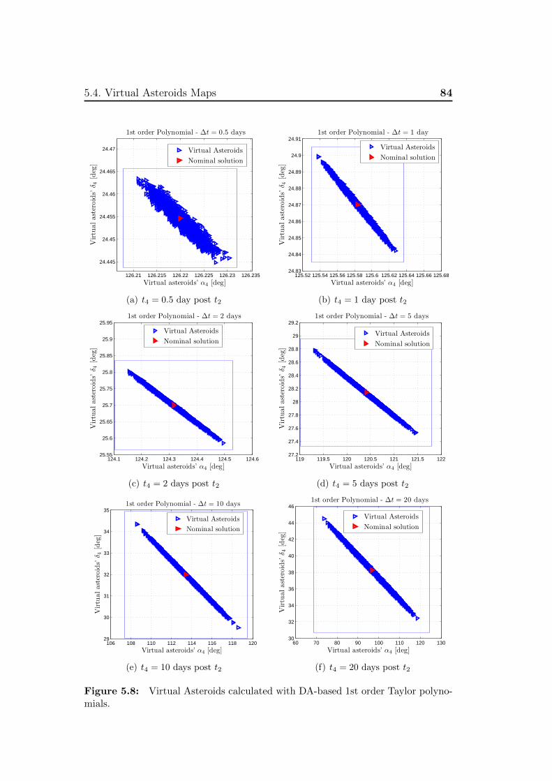
5.4. Virtual Asteroids Maps 84
126.21 126.215 126.22 126.225 126.23 126.235
24.445
24.45
24.455
24.46
24.465
24.47
Virtual asteroids’ α4 [deg]
Virtu
alast
eroid
s’δ 4
[deg
]
1st order Polynomial - Δt = 0.5 days
Virtual Asteroids
Nominal solution
(a) t4 = 0.5 day post t2
125.52 125.54 125.56 125.58 125.6 125.62 125.64 125.66 125.6824.83
24.84
24.85
24.86
24.87
24.88
24.89
24.9
24.91
Virtual asteroids’ α4 [deg]V
irtu
alast
eroid
s’δ 4
[deg
]
1st order Polynomial - Δt = 1 day
Virtual Asteroids
Nominal solution
(b) t4 = 1 day post t2
124.1 124.2 124.3 124.4 124.5 124.625.55
25.6
25.65
25.7
25.75
25.8
25.85
25.9
25.95
Virtual asteroids’ α4 [deg]
Virtu
alast
eroid
s’δ 4
[deg
]
1st order Polynomial - Δt = 2 days
Virtual Asteroids
Nominal solution
(c) t4 = 2 days post t2
119 119.5 120 120.5 121 121.5 12227.2
27.4
27.6
27.8
28
28.2
28.4
28.6
28.8
29
29.2
Virtual asteroids’ α4 [deg]
Virtu
alast
eroid
s’δ 4
[deg
]
1st order Polynomial - Δt = 5 days
Virtual Asteroids
Nominal solution
(d) t4 = 5 days post t2
106 108 110 112 114 116 118 12029
30
31
32
33
34
35
Virtual asteroids’ α4 [deg]
Virtu
alast
eroid
s’δ 4
[deg
]
1st order Polynomial - Δt = 10 days
Virtual Asteroids
Nominal solution
(e) t4 = 10 days post t2
60 70 80 90 100 110 120 13030
32
34
36
38
40
42
44
46
Virtual asteroids’ α4 [deg]
Virtu
alast
eroid
s’δ 4
[deg
]
1st order Polynomial - Δt = 20 days
Virtual Asteroids
Nominal solution
(f) t4 = 20 days post t2
Figure 5.8: Virtual Asteroids calculated with DA-based 1st order Taylor polyno-mials.
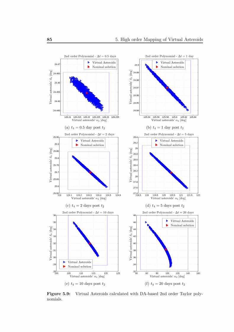
85 5. High order Mapping of Virtual Asteroids
126.21 126.215 126.22 126.225 126.23 126.235
24.445
24.45
24.455
24.46
24.465
24.47
Virtual asteroids’ α4 [deg]
Virtu
alast
eroid
s’δ 4
[deg
]
2nd order Polynomial - Δt = 0.5 days
Virtual Asteroids
Nominal solution
(a) t4 = 0.5 day post t2
125.54 125.56 125.58 125.6 125.62 125.64
24.84
24.85
24.86
24.87
24.88
24.89
24.9
Virtual asteroids’ α4 [deg]
Virtu
alast
eroid
s’δ 4
[deg
]
2nd order Polynomial - Δt = 1 day
Virtual Asteroids
Nominal solution
(b) t4 = 1 day post t2
124 124.1 124.2 124.3 124.4 124.5 124.625.55
25.6
25.65
25.7
25.75
25.8
25.85
25.9
25.95
Virtual asteroids’ α4 [deg]
Virtu
alast
eroid
s’δ 4
[deg
]
2nd order Polynomial - Δt = 2 days
Virtual Asteroids
Nominal solution
(c) t4 = 2 days post t2
118.5 119 119.5 120 120.5 121 121.5 12227.4
27.6
27.8
28
28.2
28.4
28.6
28.8
29
29.2
29.4
Virtual asteroids’ α4 [deg]
Virtu
alast
eroid
s’δ 4
[deg
]2nd order Polynomial - Δt = 5 days
Virtual Asteroids
Nominal solution
(d) t4 = 5 days post t2
100 105 110 115 120 12528
29
30
31
32
33
34
35
36
Virtual asteroids’ α4 [deg]
Virtu
alast
eroid
s’δ 4
[deg
]
2nd order Polynomial - Δt = 10 days
Virtual Asteroids
Nominal solution
(e) t4 = 10 days post t2
40 60 80 100 120 140 16032
34
36
38
40
42
44
46
48
Virtual asteroids’ α4 [deg]
Virtu
alast
eroid
s’δ 4
[deg
]
2nd order Polynomial - Δt = 20 days
Virtual Asteroids
Nominal solution
(f) t4 = 20 days post t2
Figure 5.9: Virtual Asteroids calculated with DA-based 2nd order Taylor poly-nomials.
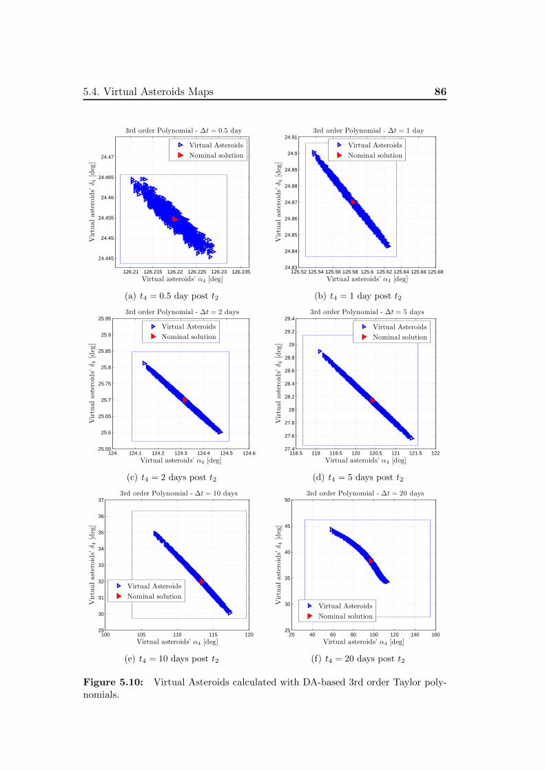
5.4. Virtual Asteroids Maps 86
126.21 126.215 126.22 126.225 126.23 126.235
24.445
24.45
24.455
24.46
24.465
24.47
Virtual asteroids’ α4 [deg]
Virtu
alast
eroid
s’δ 4
[deg
]
3rd order Polynomial - Δt = 0.5 day
Virtual Asteroids
Nominal solution
(a) t4 = 0.5 day post t2
125.52 125.54 125.56 125.58 125.6 125.62 125.64 125.66 125.6824.83
24.84
24.85
24.86
24.87
24.88
24.89
24.9
24.91
Virtual asteroids’ α4 [deg]V
irtu
alast
eroid
s’δ 4
[deg
]
3rd order Polynomial - Δt = 1 day
Virtual Asteroids
Nominal solution
(b) t4 = 1 day post t2
124 124.1 124.2 124.3 124.4 124.5 124.625.55
25.6
25.65
25.7
25.75
25.8
25.85
25.9
25.95
Virtual asteroids’ α4 [deg]
Virtu
alast
eroid
s’δ 4
[deg
]
3rd order Polynomial - Δt = 2 days
Virtual Asteroids
Nominal solution
(c) t4 = 2 days post t2
118.5 119 119.5 120 120.5 121 121.5 12227.4
27.6
27.8
28
28.2
28.4
28.6
28.8
29
29.2
29.4
Virtual asteroids’ α4 [deg]
Virtu
alast
eroid
s’δ 4
[deg
]
3rd order Polynomial - Δt = 5 days
Virtual Asteroids
Nominal solution
(d) t4 = 5 days post t2
100 105 110 115 12029
30
31
32
33
34
35
36
37
Virtual asteroids’ α4 [deg]
Virtu
alast
eroid
s’δ 4
[deg
]
3rd order Polynomial - Δt = 10 days
Virtual Asteroids
Nominal solution
(e) t4 = 10 days post t2
20 40 60 80 100 120 140 16025
30
35
40
45
50
Virtual asteroids’ α4 [deg]
Virtu
alast
eroid
s’δ 4
[deg
]
3rd order Polynomial - Δt = 20 days
Virtual Asteroids
Nominal solution
(f) t4 = 20 days post t2
Figure 5.10: Virtual Asteroids calculated with DA-based 3rd order Taylor poly-nomials.
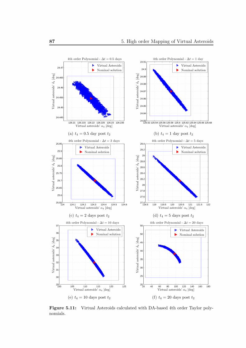
87 5. High order Mapping of Virtual Asteroids
126.21 126.215 126.22 126.225 126.23 126.235
24.445
24.45
24.455
24.46
24.465
24.47
Virtual asteroids’ α4 [deg]
Virtu
alast
eroid
s’δ 4
[deg
]
4th order Polynomial - Δt = 0.5 days
Virtual Asteroids
Nominal solution
(a) t4 = 0.5 day post t2
125.52 125.54 125.56 125.58 125.6 125.62 125.64 125.66 125.6824.83
24.84
24.85
24.86
24.87
24.88
24.89
24.9
24.91
Virtual asteroids’ α4 [deg]
Virtu
alast
eroid
s’δ 4
[deg
]
4th order Polynomial - Δt = 1 day
Virtual Asteroids
Nominal solution
(b) t4 = 1 day post t2
124 124.1 124.2 124.3 124.4 124.5 124.625.55
25.6
25.65
25.7
25.75
25.8
25.85
25.9
25.95
Virtual asteroids’ α4 [deg]
Virtu
alast
eroid
s’δ 4
[deg
]
4th order Polynomial - Δt = 2 days
Virtual Asteroids
Nominal solution
(c) t4 = 2 days post t2
118.5 119 119.5 120 120.5 121 121.5 12227.4
27.6
27.8
28
28.2
28.4
28.6
28.8
29
29.2
29.4
Virtual asteroids’ α4 [deg]
Virtu
alast
eroid
s’δ 4
[deg
]4th order Polynomial - Δt = 5 days
Virtual Asteroids
Nominal solution
(d) t4 = 5 days post t2
100 105 110 115 120 12529
30
31
32
33
34
35
36
37
Virtual asteroids’ α4 [deg]
Virtu
alast
eroid
s’δ 4
[deg
]
4th order Polynomial - Δt = 10 days
Virtual Asteroids
Nominal solution
(e) t4 = 10 days post t2
20 40 60 80 100 120 140 160 18020
25
30
35
40
45
50
55
Virtual asteroids’ α4 [deg]
Virtu
alast
eroid
s’δ 4
[deg
]
4th order Polynomial - Δt = 20 days
Virtual Asteroids
Nominal solution
(f) t4 = 20 days post t2
Figure 5.11: Virtual Asteroids calculated with DA-based 4th order Taylor poly-nomials.
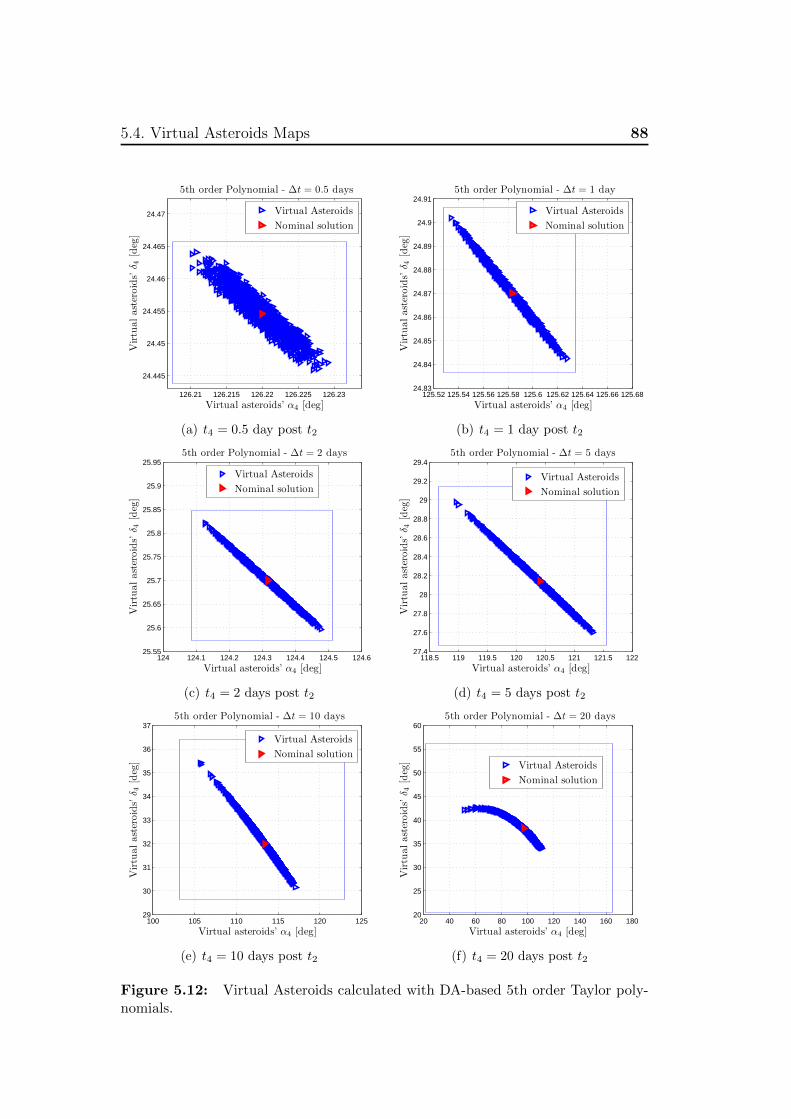
5.4. Virtual Asteroids Maps 88
126.21 126.215 126.22 126.225 126.23
24.445
24.45
24.455
24.46
24.465
24.47
Virtual asteroids’ α4 [deg]
Virtu
alast
eroid
s’δ 4
[deg
]
5th order Polynomial - Δt = 0.5 days
Virtual Asteroids
Nominal solution
(a) t4 = 0.5 day post t2
125.52 125.54 125.56 125.58 125.6 125.62 125.64 125.66 125.6824.83
24.84
24.85
24.86
24.87
24.88
24.89
24.9
24.91
Virtual asteroids’ α4 [deg]V
irtu
alast
eroid
s’δ 4
[deg
]
5th order Polynomial - Δt = 1 day
Virtual Asteroids
Nominal solution
(b) t4 = 1 day post t2
124 124.1 124.2 124.3 124.4 124.5 124.625.55
25.6
25.65
25.7
25.75
25.8
25.85
25.9
25.95
Virtual asteroids’ α4 [deg]
Virtu
alast
eroid
s’δ 4
[deg
]
5th order Polynomial - Δt = 2 days
Virtual Asteroids
Nominal solution
(c) t4 = 2 days post t2
118.5 119 119.5 120 120.5 121 121.5 12227.4
27.6
27.8
28
28.2
28.4
28.6
28.8
29
29.2
29.4
Virtual asteroids’ α4 [deg]
Virtu
alast
eroid
s’δ 4
[deg
]
5th order Polynomial - Δt = 5 days
Virtual Asteroids
Nominal solution
(d) t4 = 5 days post t2
100 105 110 115 120 12529
30
31
32
33
34
35
36
37
Virtual asteroids’ α4 [deg]
Virtu
alast
eroid
s’δ 4
[deg
]
5th order Polynomial - Δt = 10 days
Virtual Asteroids
Nominal solution
(e) t4 = 10 days post t2
20 40 60 80 100 120 140 160 18020
25
30
35
40
45
50
55
60
Virtual asteroids’ α4 [deg]
Virtu
alast
eroid
s’δ 4
[deg
]
5th order Polynomial - Δt = 20 days
Virtual Asteroids
Nominal solution
(f) t4 = 20 days post t2
Figure 5.12: Virtual Asteroids calculated with DA-based 5th order Taylor poly-nomials.
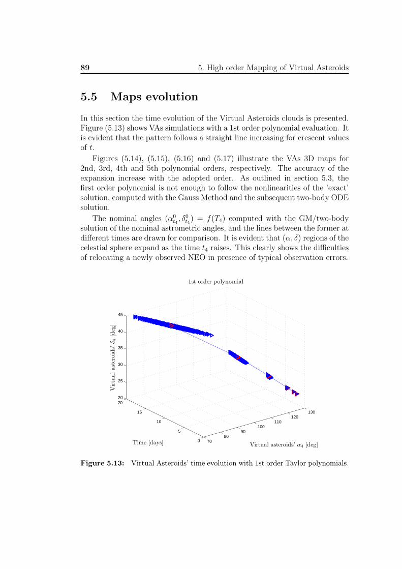
89 5. High order Mapping of Virtual Asteroids
5.5 Maps evolution
In this section the time evolution of the Virtual Asteroids clouds is presented.Figure (5.13) shows VAs simulations with a 1st order polynomial evaluation. Itis evident that the pattern follows a straight line increasing for crescent valuesof t.
Figures (5.14), (5.15), (5.16) and (5.17) illustrate the VAs 3D maps for2nd, 3rd, 4th and 5th polynomial orders, respectively. The accuracy of theexpansion increase with the adopted order. As outlined in section 5.3, thefirst order polynomial is not enough to follow the nonlinearities of the ’exact’solution, computed with the Gauss Method and the subsequent two-body ODEsolution.
The nominal angles (α0t4, δ0t4) = f(T4) computed with the GM/two-body
solution of the nominal astrometric angles, and the lines between the former atdifferent times are drawn for comparison. It is evident that (α, δ) regions of thecelestial sphere expand as the time t4 raises. This clearly shows the difficultiesof relocating a newly observed NEO in presence of typical observation errors.
7080
90100
110120
130
0
5
10
15
2020
25
30
35
40
45
Virtual asteroids’ α4 [deg]
1st order polynomial
Time [days]
Virtu
alast
eroid
s’δ 4
[deg
]
Figure 5.13: Virtual Asteroids’ time evolution with 1st order Taylor polynomials.
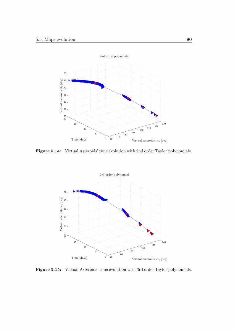
5.5. Maps evolution 90
6070
8090
100110
120130
0
5
10
15
2020
25
30
35
40
45
50
Virtual asteroids’ α4 [deg]
2nd order polynomial
Time [days]
Virtu
alast
eroid
s’δ 4
[deg
]
Figure 5.14: Virtual Asteroids’ time evolution with 2nd order Taylor polynomials.
4060
80100
120140
0
5
10
15
2020
25
30
35
40
45
Virtual asteroids’ α4 [deg]
3rd order polynomial
Time [days]
Virtu
alast
eroid
s’δ 4
[deg
]
Figure 5.15: Virtual Asteroids’ time evolution with 3rd order Taylor polynomials.
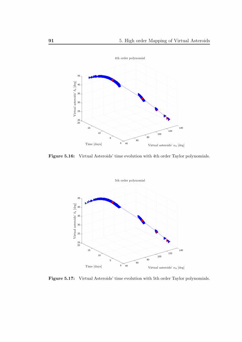
91 5. High order Mapping of Virtual Asteroids
4060
80100
120140
0
5
10
15
2020
25
30
35
40
45
Virtual asteroids’ α4 [deg]
4th order polynomial
Time [days]
Virtu
alast
eroid
s’δ 4
[deg
]
Figure 5.16: Virtual Asteroids’ time evolution with 4th order Taylor polynomials.
4060
80100
120140
0
5
10
15
2020
25
30
35
40
45
Virtual asteroids’ α4 [deg]
5th order polynomial
Time [days]
Virtu
alast
eroid
s’δ 4
[deg
]
Figure 5.17: Virtual Asteroids’ time evolution with 5th order Taylor polynomials.
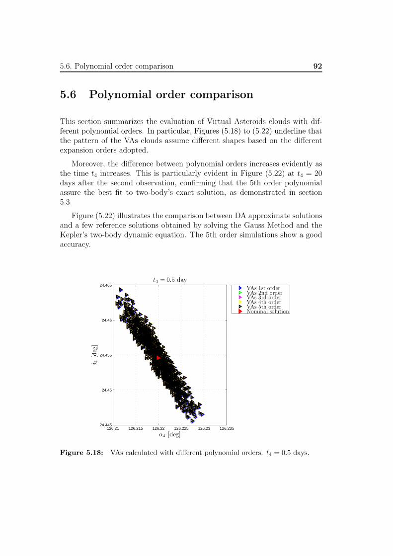
5.6. Polynomial order comparison 92
5.6 Polynomial order comparison
This section summarizes the evaluation of Virtual Asteroids clouds with dif-ferent polynomial orders. In particular, Figures (5.18) to (5.22) underline thatthe pattern of the VAs clouds assume different shapes based on the differentexpansion orders adopted.
Moreover, the difference between polynomial orders increases evidently asthe time t4 increases. This is particularly evident in Figure (5.22) at t4 = 20days after the second observation, confirming that the 5th order polynomialassure the best fit to two-body’s exact solution, as demonstrated in section5.3.
Figure (5.22) illustrates the comparison between DA approximate solutionsand a few reference solutions obtained by solving the Gauss Method and theKepler’s two-body dynamic equation. The 5th order simulations show a goodaccuracy.
126.21 126.215 126.22 126.225 126.23 126.23524.445
24.45
24.455
24.46
24.465
α4 [deg]
δ 4[d
eg]
t4 = 0.5 day
VAs 1st orderVAs 2nd orderVAs 3rd orderVAs 4th orderVAs 5th orderNominal solution
Figure 5.18: VAs calculated with different polynomial orders. t4 = 0.5 days.
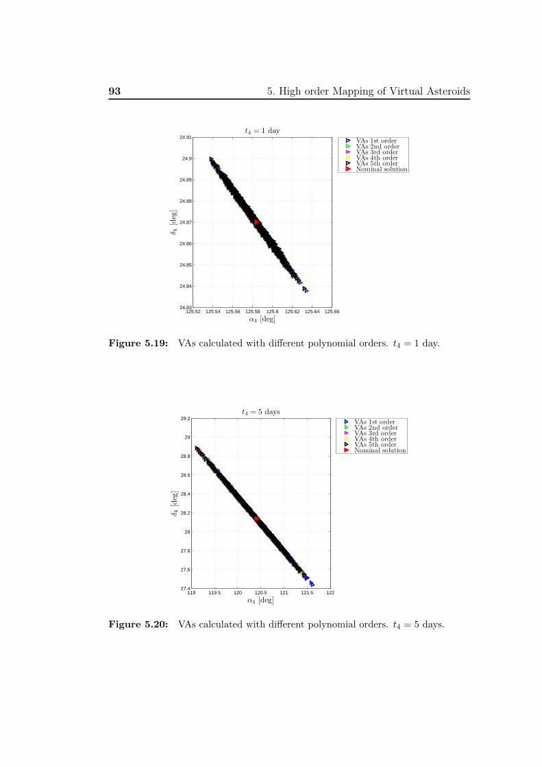
93 5. High order Mapping of Virtual Asteroids
125.52 125.54 125.56 125.58 125.6 125.62 125.64 125.6624.83
24.84
24.85
24.86
24.87
24.88
24.89
24.9
24.91
α4 [deg]
δ 4[d
eg]
t4 = 1 day
VAs 1st orderVAs 2nd orderVAs 3rd orderVAs 4th orderVAs 5th orderNominal solution
Figure 5.19: VAs calculated with different polynomial orders. t4 = 1 day.
119 119.5 120 120.5 121 121.5 12227.4
27.6
27.8
28
28.2
28.4
28.6
28.8
29
29.2
α4 [deg]
δ 4[d
eg]
t4 = 5 days
VAs 1st orderVAs 2nd orderVAs 3rd orderVAs 4th orderVAs 5th orderNominal solution
Figure 5.20: VAs calculated with different polynomial orders. t4 = 5 days.
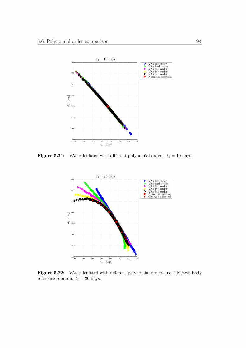
5.6. Polynomial order comparison 94
106 108 110 112 114 116 118 12029
30
31
32
33
34
35
36
α4 [deg]
δ 4[d
eg]
t4 = 10 days
VAs 1st orderVAs 2nd orderVAs 3rd orderVAs 4th orderVAs 5th orderNominal solution
Figure 5.21: VAs calculated with different polynomial orders. t4 = 10 days.
50 60 70 80 90 100 110 12032
34
36
38
40
42
44
46
α4 [deg]
δ 4[d
eg]
t4 = 20 days
VAs 1st orderVAs 2nd orderVAs 3rd orderVAs 4th orderVAs 5th orderNominal solutionGM/2-bodies sol
Figure 5.22: VAs calculated with different polynomial orders and GM/two-bodyreference solution. t4 = 20 days.
Chapter 6
Conclusions and Future work
The Differential Algebraic approach to describe the manifolds of so-called Vir-tual Asteroids has shown a good efficiency for computing the approximate so-lution of the astrometric positions of an asteroid observed almost three timesin a limited time interval.
More specifically, 5th-order Taylor polynomials can be computed to accu-rately map initial clouds of possible asteroid states forward in time. Thesemaps are used to endorse the portion of the sky to be observed to track a spe-cific ’target’, and then optimize the telescope observation scanning. Moreover,the computing time to generate high order polynomials, and the time to evalu-ate these polynomials for perturbed parameters is very limited if compared toGM/two-body solution. According to the simulations presented in this work,CPU times to generate 5th order approximate solution in COSY INFINITY isabout to 5-6 seconds, while the evaluation of 1000 samples of randomly gen-erated initial condition in MATLAB environment is limited to 2-3 seconds. Incontrast, each GM evaluation needs a CPU time of 0.2-0.5 seconds, for a totalof 200-500 seconds.
It is evident that this approach is not only generally reliable, but can bealso adapted to the intrinsic precision of Earth-based telescopes. This methodrequires only to update the value of the standard deviation σ used to generatethe Ns samples, in this way evaluating the astrometric position at any time t4after the observation phase.
The errors between the GM/two-body dynamics and the approximate DA-based solution have been calculated. More specifically 20 days after the secondobservation, 5th order polynomials present a maximum error of 1.5·10−6 degwhile evaluating the topocentric Right Ascension and of 7·10−4 deg while eval-uating the declination. After 20 days, the maps assume a little distortion
95
96
and the difference between the polynomials’ patterns increases. This indicatesthe limits of the precision of 5th order polynomials and paves the way to anextended analysis towards higher orders.
It is worth observing that all errors are evaluated in the two-body Sun-asteroid dynamical model. A refined dynamical analysis in a more completedynamical model must be taken into account to confirm the accuracy of the5th order polynomials.
Possible extensions of this work should be:
• the study of the evolution of NEOs’ astrometry maps with higher orderpolynomials, to investigate the errors between the two-body model andthe DA-approximation for t4 > 20 days after the preliminary observation;
• the study of the problem within the N -body dynamical model;
• the study of the accuracy respect to the time span between the prelimi-nary observations;
• the development of appropriate strategies to optimize the portion of thecelestial sphere to be observed at the presence of DA-based indications.
Acronyms
2BP Two Body Problem
AU Astronomic Unit
CCD Charged Coupled Device
CED Close Approach Distance
COE Classical Orbital Elements
CPU Central Processing Unit
DA Differential Algebra
dec Declination
DLR Deutsches Zentrum fur Luft- und Raumfahrt
EARN European Asteroids Research Node
GM Gauss Method for orbital determination
IAU International Astronomical Union
INAF Istituto Nazionale di Astrofisica
JD Julian Date
JD2000 Julian Date from 1st January 2000
JPL Jet Propulsion Laboratory
JSGA Japanese Space Guard Association
LDB Linear Dominated Bounder
LONEOS Lowell Observatory Near-Earth Object Search
LSST Large Synoptic Survey Telescope97
98
LST Local Sidereal Time
MIT Massachusetts Institute of Technology
MPC Minor Planets Center
MSU Michigan State University
NASA National Aeronautic and Space Administration
NEA Near Earth Asteroid
NEAT Near Earth Asteroid Tracking
NEC Near Earth Comet
NEO Near Earth Object
NEODyS Near Earth Objects Dynamics Site - Pisa
NEOSSat Near-Earth-Object Surveillance Satellite
NEOWISE Near-Earth-Object WISE
ODE Ordinary Differential Equation
PHA Potentially Hazardous Asteroid
RA Right Ascension
TM Taylor Model
VA Virtual Asteroid
VLBI Very Long Baseline Interferometry
WISE Wide-field Infrared Survey Explorer
Bibliography
[1] Howard D. Curtis, Orbital Mechanics for Engineering Students, Else-vier BH, New York, United States, 2005.
[2] Pierluigi Di Lizia, Robust Space Trajectory and Space System De-sign using Differential Algebra, Tesi di Dottorato di Ricerca, XX Ciclo,Politecnico di Milano, Italia, 2008.
[3] M. Berz and K. Makino, COSY INFINITY 9.0 Programmer’s Manual,MSU Report MSUHEP 060803, Michigan State University, United States,2006.
[4] Mario Carpino, Introduzione ai metodi di calcolo di Effemeridi e de-terminazione orbitale, Osservatorio Astronomico di Brera, Milano, Italia,2010.
[5] P. Di Lizia, R. Armellin and M.Lavagna, Application of high or-der expansions of two-point boundary value problems to astrodynamics,Celestial Mechanics and Dynamical Astronomy Journal, Springer, 2008.
[6] P. Di Lizia, R. Armellin, F. Bernelli-Zazzera, M. Berz, As-teroid Close Encounters Characterization using Differential Algebra: theCase of Apophis, Celestial Mechanics and Dynamical Astronomy Journal,Springer, 2010.
[7] O.P. Bykov, V.N. L’vov, I.S. Izmailov, G.R. Kastel, An accuracyestimation of the World CCD asteroid observations in the years 1999-2005,Planetary and Space Science Journal, Elsevier, 2008.
[8] Jet Propulsion Laboratory, Website of JPL,http://neo.jpl.nasa.gov/, Discovery statistics, january 2011.
99
BIBLIOGRAPHY 100
[9] E. Myles Standish and James G. Williams, Models for high-precision spacecraft and planetary and lunar ephemerides, Proceedingsof the International Astronomical Union, 2006.
[10] Richard H. Battin, An Introduction to the Mathematics and Methodsof Astrodynamics, AIAA Education Series, 1999.
[11] Kyoko Makino, Rigorous Analysis of Nonlinear Motion in Particle Ac-celerators, Ph.D. Thesis, Michigan State University, East Lansing, Michi-gan, USA, 1998.