
POLITECNICO DI MILANO Engineering · Chiara Pasquino Matr. 733945 ... Politecnico di Milano, Marco...
130
POLITECNICO DI MILANO Master Degree in Materials Engineering ELECTRON STIMULATED DESORPTION OF OFE COPPER FOR PARTICLE ACCELERATORS Advisors: Prof. Marco Beghi Correlatore(i): Sergio Calatroni Chiara Pasquino Matr. 733945 Submitted in partial fulfilment of the requirements For the degree of Master of Science in Materials Engineering, Politecnico di Milano, 2011 Geneva, Switzerland
Transcript of POLITECNICO DI MILANO Engineering · Chiara Pasquino Matr. 733945 ... Politecnico di Milano, Marco...
POLITECNICO DI MILANO
Master Degree in Materials Engineering
ELECTRON STIMULATED DESORPTION OF OFE
COPPER FOR PARTICLE ACCELERATORS
Advisors: Prof. Marco Beghi
Correlatore(i): Sergio Calatroni
Chiara Pasquino Matr. 733945
Submitted in partial fulfilment of the requirements
For the degree of Master of Science in Materials Engineering,
Politecnico di Milano, 2011
Geneva, Switzerland

ii
Acknowledgement
I would like to acknowledge, first of all, my CERN supervisor, Sergio Calatroni, for his
help and experience and for guiding me in this work in all its aspects: from the
hardware troubleshooting in the laboratory to the proficient discussions about
theoretical models and experimental data analysis. I’d like to thank my supervisor at
Politecnico di Milano, Marco Beghi, as well, for his support during this year at CERN
and for my future career.
Furthermore, I’d like to acknowledge Mauro Taborelli and Walter Wuensch for
the useful discussions and remarks, always intended to the improvement and
encouragement; Ana Rocio Santiago Kern for her fundamental helping and
teaching; Helga Timko for the interesting talking and discussions, as well as Jan
Kovermann and Markus Aicheler.
I’d like to thank, then, everybody that helped me out in the laboratory: Ivo
Wevers for his experience and really nice talks; Luigi Leggiero and Paul Garritty for
the many changes I’ve asked them to do at the hardware of the experimental
system, for their kindness and professionalism; Pawel Modrzynski for helping me in
the lab and for the nice chats we had during this year; Donat Holzer for his helping
me out; Wilhelmus Vollenberg and Holger Neupert for their experience and
assistance.
Last but not least, my family and my fiancé Claudio for the support they gave
me during the University and during this year abroad, and all my old and new
friends that are the special ingredient making this year a wonderful experience.
iii
Abstract
This master thesis has been developed at CERN, European Center for Nuclear
Research, in the framework of CLIC, Compact Linear Collider project. CLIC is aiming
at designing a future electron – positron linear collider in order to explore a new
energy region beyond the one provided by the LHC, being a step forward in particle
physics research.
CLIC project involves many experts at CERN covering different areas: from Radio
Frequency design of the accelerating structures to advanced civil engineering for
the alignment of the whole accelerator; from the design of the RF power supply to
materials and vacuum studies.
The work hereafter described concerns the study of materials behavior in the
accelerating structures and their influence on static and dynamic vacuum: the high
gradient (≈ 100 MV/m) characterizing the accelerating structures is the triggering of
several physical phenomena that lead to local bursts of pressures. Thus, these
phenomena are the main cause of a possible particle beam – residual molecules
interaction, causing a defocusing of the beam and a loss of luminosity. Several
materials have been tested up to now in experimental sets up built ad hoc at CERN:
the main candidate is OFE – Oxygen Free Electronic grade Copper.
In order to study the dynamic vacuum behavior into deep, a new experimental
set up has been built, aiming at measuring the Desorption Yield of several copper
samples characterized by different manufacturing procedures: the main goal would
be to identify the best production flow leading to a ‘high gradient resistant’ Copper.
The First Chapter briefly describes what CLIC project is, which the main
components are and the issues that a 50 km long accelerator has to deal with.
In the Second Chapter a theoretical description of the physical phenomena
leading to dynamic vacuum effects is provided. Breakdowns studies are an ongoing
activity since 2001 while Electron Stimulated Desorption studies started with this
Master thesis.
iv
The Third Chapter is concerning the manufacturing flow of copper samples to
be tested from the dynamic vacuum point of view. In addition, a diffusion profile
analysis has been developed in order to predict the impact of several heat
treatments on copper samples.
The Fourth Chapter describes into details the whole experimental set up built in
order to measure the above mentioned Desorption Yield on unbaked copper
sample at high electron energy (KeV): starting from the hardware needed
(instruments, vacuum chambers, electron source…) to the software that controls
the instrumentation. A description of the upgrades done is also provided.
The experimental data collected up to now from the new experimental set‐up
are analyzed in the Fifth Chapter. The first data are related to spare copper samples
tested at the start up of the system.
In conclusion, the dynamic vacuum effects in CLIC accelerating structures have
been studied and a new experimental set up has been built in order to measure the
Desorption Yield of several Copper samples at high electron energy. First
experimental data are provided but the whole sample testing campaign will be
developed in the near future.
v
Abstract
Il seguente lavoro di laurea è stato sviluppato al CERN, Centro Europeo per la
Ricerca Nucleare, nell’ambito del progetto CLIC, Compact Linear Collider. CLIC si
prefigge di effettuare il design di un futuro acceleratore lineare per collisioni
elettrone – positrone, di modo da permettere l’esplorazione di una nuova regione
di energie che si colloca al di là di quella accessibile grazie all’LHC, Large Hidron
Collider.
Il progetto CLIC coinvolge un considerevole numero di scenziati esperti in
diversi domini: dal design della Radio Frequenza delle strutture acceleranti alla più
avanzata ingegneria civile per l’allineamento dell’intero acceleratore; dal design
della linea di potenza di Radio Frequenza allo studio del comportamento dei
materiali impiegati in condizioni di alto vuoto (UHV – Ultra High Vacuum).
Il presente elaborato concerne lo studio del comportamento dei materiali
impiegati nelle strutture acceleranti e la loro influenza sul vuoto statico e dinamico:
l’elevato gradiente che caratterizza le strutture acceleranti ( ~ 100 MV/m) innesca
diversi fenomeni fisici che inducono innalzamenti locali della pressione. Questi
fenomeni sono la causa principale di possibili interazioni tra le particelle del fascio e
le molecole rilasciate dalla superficie della cavità accelerante, causando la
defocalizzazione del fascio e una conseguente perdita di luminosità. Finora, diversi
materiali sono stati testati grazie ai set – up sperimentali costruiti appositamente al
CERN: il principale candidato per le strutture acceleranti è il rame OFE – Oxygen
Free Electronic grade.
Uno studio approfondito relativo al vuoto dinamico ha comportato la
costruzione di un nuovo set – up sperimentale volto alla misura del coefficiente di
desorbimento di numerosi provini in rame. Essi sono caratterizzati da diverse
procedure di produzione che si rifanno alle modalità di lavorazione meccanica, ai
trattamenti superficiali e termici tipici delle strutture acceleranti. L’obiettivo
principale è, pertanto, individuare il migliore processo di produzione che porti ad
vi
ottenere una superficie di rame che sia resistente all’alto gradiente di
accelerazione.
Il primo capitolo descrive brevemente il progetto CLIC, i suoi componenti
principali e le problematiche che si devono affrontare nel design di un acceleratore
lungo 50 km.
Nel secondo capitolo è riportata la descrizione teorica dei fenomeni fisici che
inducono la problematica del vuoto dinamico. Studi relativi ai breakdowns
costituiscono un’attività di ricerca consolidata ormai da anni, mentre l’analisi del
desorbimento indotto da elettroni (ESD – Electron Stimulated Desorption) ha avuto
inizio con il seguente lavoro di laurea.
Il terzo capitolo riguarda la descrizione dei trattamenti superficiali e termici
relativi ai provini di rame impiegati per la misura del coefficiente di desorbimento.
Inoltre, è riportata un’analisi dei profili di diffusione dell’Idrogeno volta a stimare
l’impatto di alcuni dei trattamenti termici sui suddetti provini.
Il quarto capitolo descrive in dettaglio il set – up sperimentale costruito per
studiare il fenomeno dell’ESD a elevate energie elettroniche (nell’ordine delle
decine di KeV): dai componenti necessari ( strumentazione, camere a vuoto, la
sorgente di elettroni...) fino ai software che permettono il controllo della
strumentazione. È riportata, inoltre, una descrizione delle migliorie apportate al
sistema.
I dati sperimentali raccolti sinora sono analizzati nel quinto capitolo: sono
relativi ad alcuni provini di rame impiegati per testare il buon funzionamento del
sistema e al primo provino appartenente alla campagna ufficiale.
In conclusione, sono stati studiati gli effetti del vuoto dinamico nelle strutture
acceleranti di CLIC e un nuovo set ‐ up sperimentale è stato costruito per misurare
il coefficiente di desorbimento indotto da elettroni ad alta energia su alcuni provini
di rame OFE. I primi dati sperimentali sono relativi a un numero ristretto di provini
mentre la completa campagna sperimentale verrà iniziata prossimamente.

vii
viii
Table of Contents
CHAPTER 1 CLIC ‐ Compact LInear Collider project ............................................... 1
CHAPTER 2 Dynamic Vacuum: an Issue for CLIC Accelerating Structures ............ 10
2.1 Dynamic Vacuum Sources: Breakdowns and Dark Currents ....................... 12
2.1.1 Breakdowns Studies .............................................................................. 12
2.1.2 Experimental Set‐up and Results .......................................................... 14
2.1.3 Breakdown Dynamic Vacuum Simulations ........................................... 19
2.1.4 Static Vacuum analysis ......................................................................... 21
2.1.5 Dark Current Studies ............................................................................. 22
2.2 Electron Stimulated Desorption: fundamental mechanisms ...................... 24
2.2.1 The Menzel‐Gomer‐Redhead Model ..................................................... 24
2.2.2 Antoniewicz’s model ............................................................................. 27
2.2.3 Gortel’s model ...................................................................................... 31
2.3 Interaction of electrons with matter ........................................................... 35
2.3.1 Energetic electrons ............................................................................... 35
2.4 Electron Stimulated Desorption: Desorption Yield ..................................... 38
2.4.1 Determination of the Desorption Yield ................................................. 39
2.4.2 Conductance and volume throughput .................................................. 43
CHAPTER 3 Copper samples specifications ........................................................ 46
3.1 Cleaning Procedures .................................................................................... 47
3.2 Bonding Cycles Specifications ...................................................................... 48
3.3 Diffusion Profile Calculations ....................................................................... 54
3.3.1 Copper – Hydrogen interactions ........................................................... 54
3.3.2 Mathematics of Diffusion ..................................................................... 56
3.3.3 Calculations .......................................................................................... 58
3.4 Copper Samples Specifications .................................................................... 65
CHAPTER 4 Electron Stimulated Desorption: Experimental Set‐up..................... 67
4.1 Experimental Set‐up .................................................................................... 67
4.1.1 Thermal Conductivity Gauges: PIRANI gauge ....................................... 73
4.1.2 Ionization gauges .................................................................................. 75
ix
4.1.3 Hot cathode ionization gauge: Bayard‐Alpert gauge. .......................... 76
4.1.4 Cold cathode ionization gauge: Penning gauge ................................... 79
4.1.5 RGA: Residual Gas Analyzer .................................................................. 80
4.1.6 RGA calibration ..................................................................................... 84
4.2 Pumping speeds calculations ....................................................................... 87
4.3 Thermal Analysis .......................................................................................... 89
4.4 Background Pressure ................................................................................... 91
4.5 Bake – out .................................................................................................... 92
4.6 Measurement procedure ............................................................................ 94
4.7 Sofwares : Quadstar32 & Labview ............................................................... 95
4.8 Troubleshooting and upgrades .................................................................... 97
CHAPTER 5 ESD experimental data analysis ....................................................... 99
5.1 Data Analysis ................................................................................................ 99
5.2 First ESD experimental data ...................................................................... 102
5.3 Electron energy correlation ....................................................................... 105
5.4 Experimental data for 19_PCV082C .......................................................... 107
5.5 Troubleshooting ......................................................................................... 109
CHAPTER 6 Conclusions ................................................................................... 112
BIBLIOGRAPHY ................................................................................................... 114

x
List of Figures
Figure 1: Simplified CLIC Layout. .................................................................................. 2
Figure 2: Complete CLIC Layout. .................................................................................. 3
Figure 3: Pumping System layout for CLIC. .................................................................. 4
Figure 4: Insight of a CLIC accelerating structure. ....................................................... 5
Figure 5: reference line scheme for CLIC alignment. ................................................... 5
Figure 6: Module type 1 Cooling System. .................................................................... 6
Figure 7: Cross section of the tunnel where CLIC will b installed. ............................... 7
Figure 8: a) geological investigations of the French‐Swiss region nearby CERN; b)
geological investigation, taking into account the Hearth curvature. .......................... 8
Figure 9: CLIC Test Facility 3. ....................................................................................... 9
Figure 10: CLIC accelerating structure. ...................................................................... 11
Figure 11: Triggering and sustaining of the arcing in vacuum. .................................. 13
Figure 12: Craters by SEM analysis. ........................................................................... 13
Figure 13: DC spark experimental layout. ................................................................. 14
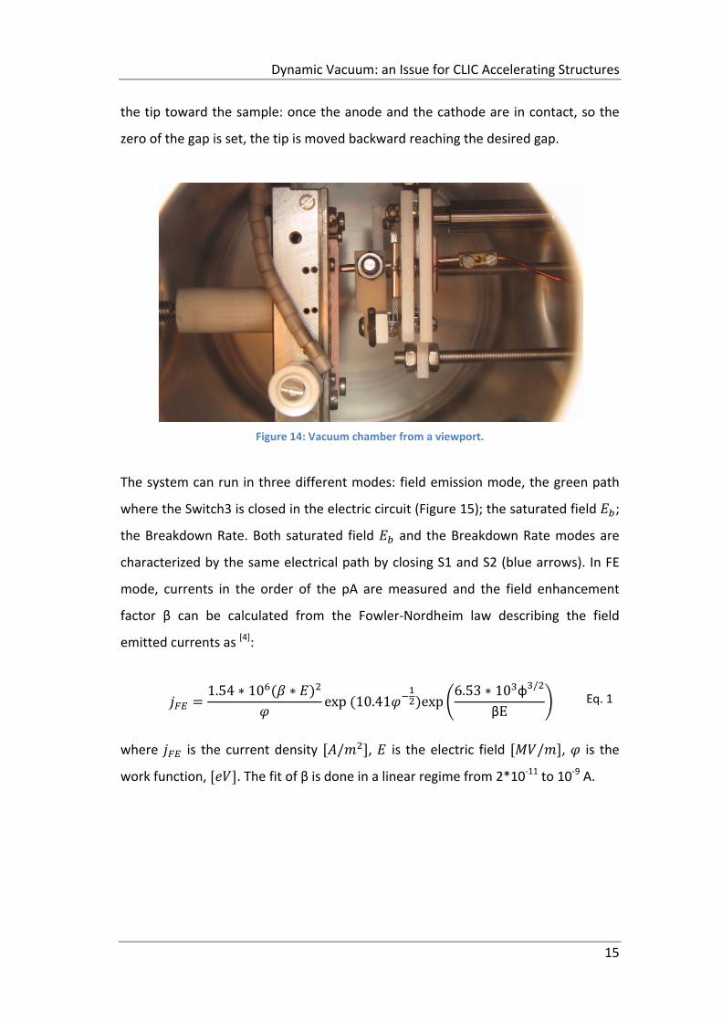
Figure 14: Vacuum chamber from a viewport. .......................................................... 15
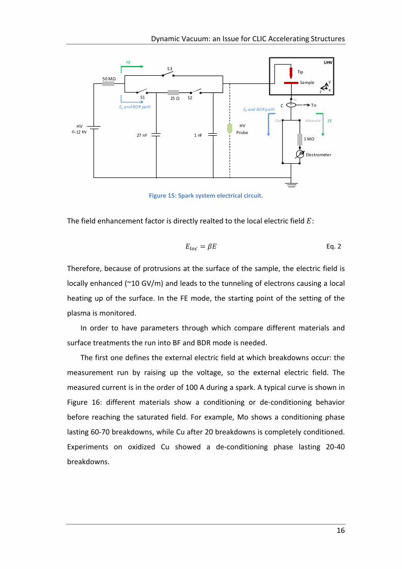
Figure 15: Spark system electrical circuit. ................................................................. 16
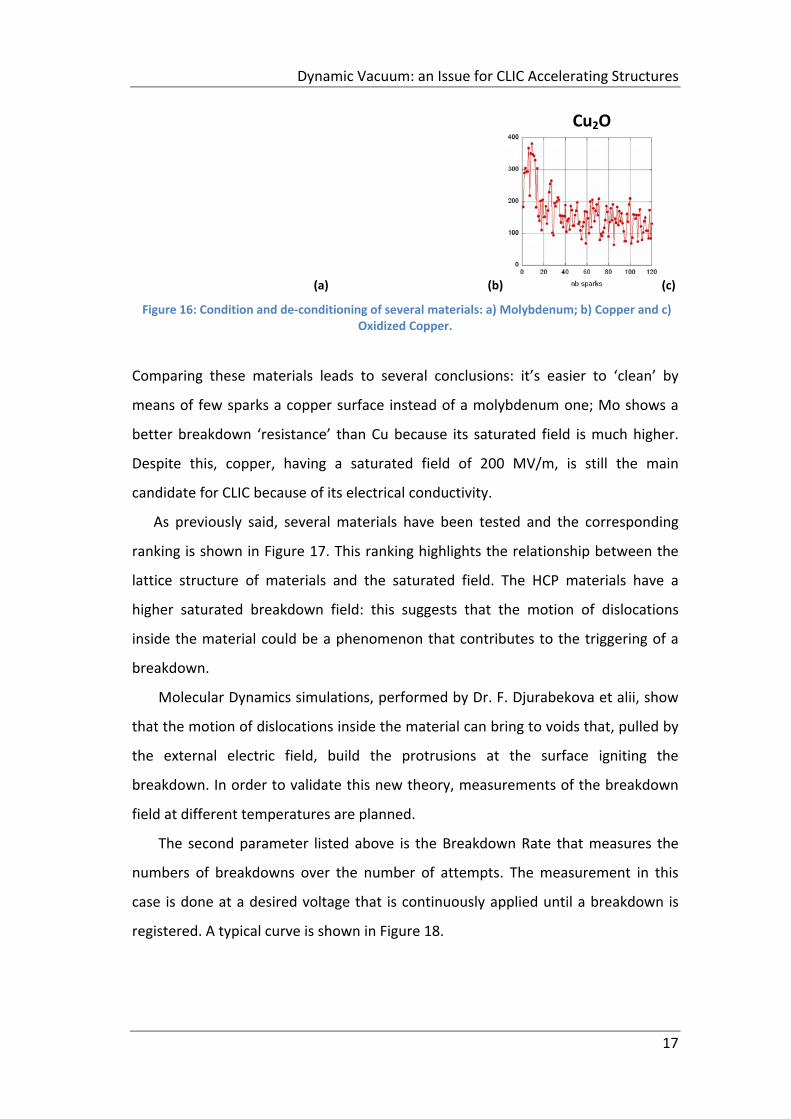
Figure 16: Condition and de‐conditioning of several materials: a) Molybdenum; b)
Copper and c) Oxidized Copper. ................................................................................ 17
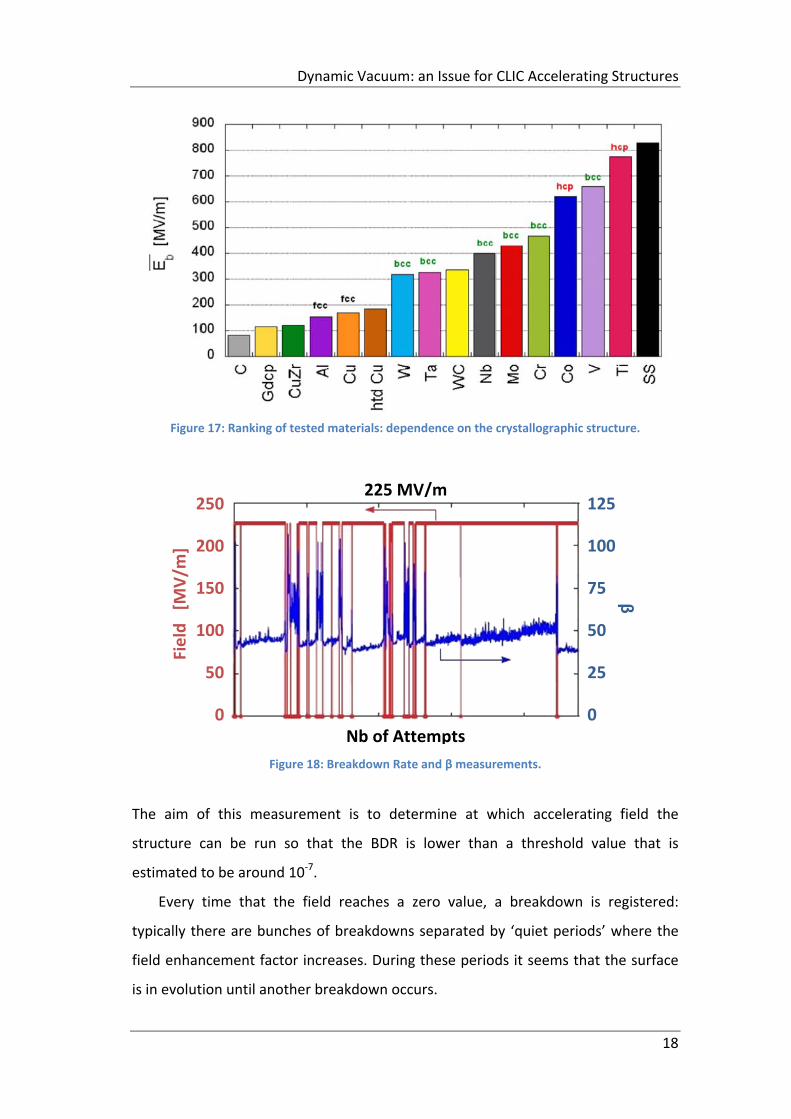
Figure 17: Ranking of tested materials: dependence on the crystallographic
structure..................................................................................................................... 18
Figure 18: Breakdown Rate and β measurements. ................................................... 18
Figure 19: The mesh of the designed accelerating structures. ................................. 21
Figure 20: Pressure profile in the middle of the accelerating structure Vs time. ..... 21
Figure 21: static pressure profile in the drive beam. ................................................. 22
Figure 22: Simplified scheme of field‐emitted electrons in the accelerating cavity. 23
Figure 23: ESD mechanism proposed by MGR .......................................................... 26
Figure 24: Antoniewicz’s ESD model for neutrals desorption. .................................. 28
Figure 25: Anoniewicz’s ESD model for ionic desorption. ......................................... 30
Figure 26: The wave function spreads out of time. ................................................... 33
Figure 27: Gortel ESD quantum – mechanical scenario. ........................................... 34
Figure 28: Kinetic energy distribution of Ar atoms desorbing from Ru(001). ........... 35
Figure 29: Cu stopping power as function of electronic energy................................ 36
Figure 30: Stopping power of species usually desorbed from a surface. .................. 37
Figure 31: Maximum Range for electrons bombarding Copper. ............................... 38
Figure 32: Scheme of a vacuum chamber with different gas loads. ......................... 40
Figure 33: Desorption Yield of several gases on non‐baked Cu @ 0.35kV. ............... 42
xi
Figure 34: Diamond Turned CLIC accelerating structure. .......................................... 47
Figure 35: Diffusion Bonding thermal cycle in vacuum. ............................................ 49
Figure 36: Diffusion Bonding thermal cycle in Argon atmosphere ........................... 49
Figure 37: Diffusion Bonding thermal cycle in Hydrogen at different pressures ...... 50
Figure 38: Insight of the bonding furnace. ................................................................ 52
Figure 39: furnace thermal treatment previous bonding (left); bonding thermal
treatment (right). ....................................................................................................... 52
Figure 40: Five‐cells bonded structure. ..................................................................... 53
Figure 41: SEM analysis of the cut bonded structure. ............................................... 53
Figure 42: solubility of Hydrogen in Copper as function of Temperature. ................ 56
Figure 43: Scheme of Hydrogen diffusion in a semi‐infinite media. ......................... 57
Figure 44: scheme of Hydrogen diffusion in a plane sheet. ...................................... 58
Figure 45: Diffusion Bonding thermal cycle under 1bar of Hydrogen. ...................... 59
Figure 46: Hydrogen Diffusion profile for a semi‐infinite media. .............................. 59
Figure 47: Hydrogen diffusion profile in space and time. ......................................... 60
Figure 48: Hydrogen diffusion profile in a plane sheet after the bonding plateau. .. 61
Figure 49: scheme of the approximation of the thermal ramp down. ...................... 62
Figure 50: Hydrogen diffusion profile in a plane sheet during the thermal ramp
down. ......................................................................................................................... 63
Figure 51: Hydrogen diffusion profile in a plane sheet at the end of the thermal
ramp down. ................................................................................................................ 63
Figure 52: Hydrogen content during the heat treatment after bonding. ................. 64
Figure 53: Drawing of a copper sample. .................................................................... 65
Figure 54: ESD system experimental set‐ up. ............................................................ 69
Figure 55: insight of the experimental set – up: lower and upper vacuum chamber.
................................................................................................................................... 69
Figure 56: ESD experimental set – up electrical circuit. ............................................ 71
Figure 57: Picture of the ESD experimental set‐up. .................................................. 72
Figure 58: Snapshot of the upper vacuum chamber. ................................................ 73
Figure 59: Scheme of the Pirani gauge heat transfer. ............................................... 74
Figure 60: Drawing of a Pirani gauge. ........................................................................ 75
Figure 61: Generalized ionization gauge. .................................................................. 76
Figure 62: Ionization cross section as function of electron energy. .......................... 77
Figure 63: First layout of a hot cathode ionization vacuum gauge. .......................... 78
Figure 64: electrical old scheme of the triode configuration. ................................... 78
Figure 65: new triode lay‐out conceived by Bayard and Alpert. ............................... 79
Figure 66: Electrode arrangement, fields, and trajectories in the Penning gauge. ... 80
Figure 67 QMS ‐ Quadrupole Mass Spectrometer lay – out. .................................... 81
Figure 68: Analog scan done with Q32. ..................................................................... 82
Figure 69: Typical desorption signal monitored by Q32 in the versus time mode. .. 84
xii
Figure 70:H2 calibration factor. .................................................................................. 86
Figure 71: N2 calibration factor. ................................................................................. 86
Figure 72: Lower vacuum chamber – highlight on the 3 vacuum resistors............... 87
Figure 73: scheme of the sample and the electron source in the lower vacuum
chamber. .................................................................................................................... 89
Figure 74: scheme of the sample and the electron source – configuration factor. .. 91
Figure 75: sojourn time of several gaseous species. ................................................. 92
Figure 76: Usual thermal cycle for vacuum systems bake – out. .............................. 93
Figure 77: bake – out scheme for the ESD experimental set – up. ........................... 93
Figure 78: Labview program snapshot. ..................................................................... 96
Figure 79: insight of the sample holder and power feedthrough. ............................ 97
Figure 80: new rod with a magnetic manipulator. .................................................... 98
Figure 81:typical ramp up shape of a desorption signal. ........................................ 100
Figure 82: typical recovering curve of a desorption signal. ..................................... 101
Figure 83: Desorption Yield experimental data for a spare copper sample @ 0.35 kV
................................................................................................................................. 103
Figure 84: Desorption Yield experimental data for a spare copper sample @ 5kV. 104
Figure 85: Desorption Yield experimental data for a spare copper sample @ 10kV.
................................................................................................................................. 105
Figure 86: Desorption Yield experimental data as function of the electron energy.
................................................................................................................................. 106
Figure 87: Desorption Yield experimental data as function of the electron energy at
1.615 e‐/cm2. ............................................................................................................. 106
Figure 88: Desorption Yield experimental data @ 10 kV for 19_PCV082C. ............ 107
Figure 89: Desorption Yield experimental data as function of electron energy for
19_PCV082C. ............................................................................................................ 108
Figure 90: Desorption Yield experimental data @ 10 kV for 19_PCV082C ............. 109
Figure 91: Desorption Yield experimental data of a spare copper sample @ 10kV.
................................................................................................................................. 109
Figure 92: Desorption Yield experimental data of a spare copper sample as function
of electron energy. ................................................................................................... 110
xiii
List of Tables
Table 1: CLIC parameters ............................................................................................. 9
Table 2: scheme of the vacuum diffusion bonding procedure .................................. 49
Table 3: scheme of the Argon diffusion bonding procedure. .................................... 50
Table 4: scheme of the Hydrogen diffusion bonding procedure both at 10 mbar & 1
bar. ............................................................................................................................. 50
Table 5: Sample campaign. ........................................................................................ 66
Table 6: RGA cracking pattern ................................................................................... 83
Table 7: gauge sensitivities. ....................................................................................... 85
Table 8: Conductance for several gases. ................................................................... 88
Table 9: Pumping speeds for several gases. .............................................................. 88
Table 10: Sample temperatures during bombardment or not. ................................. 91
Table 11: Bake ‐ out temperatures list. ..................................................................... 94
Table 12: examples of rising time ............................................................................ 100
Table 13: examples of time constants. .................................................................... 101
CLIC ‐ Compact LInear Collider project
1
CHAPTER 1
CLIC ‐ COMPACT LINEAR COLLIDER
PROJECT
The Compact LInear Collider (CLIC) is the future linear particle accelerator facility
designed at CERN, the European Center for Nuclear Research, Geneva.
CLIC is a worldwide collaboration of experts in different domains, aiming at the
development of a 50 Km length linear collider. The project involves several
important partners: the International Linear Collider project (ILC), conceived for 500
GeV collisions; the Stanford Linear Accelerator Center (SLAC) in California, US; the
High Energy Accelerator Research Organization (KeK), in Tsukuba, Japan.
CLIC is designed for electron‐positron collisions up to a multi‐TeV center‐of‐
mass energy range (the nominal one is 3 TeV). It is a challenging project since it is
the first time that a linear collider is conceived for producing such high energy
collisions, requiring a very high accelerating gradient.
This energy range is similar to the LHC’s, but, by using electrons and their
antiparticles rather than protons, physicists will gain a different perspective on the
underlying physics. It would provide, indeed, significant fundamental physics
information complementary to the LHC and a lower‐energy linear e+/e‐ collider, as a
result of its unique combination of high energy and experimental precision.
CLIC ‐ Compact LInear Collider project
2
As mentioned above, highly accelerated particles are needed for high energetic
collisions. The design of the whole linear accelerator is conceived so that an
accelerating gradient about 100 MV/m is reached in the accelerating structures:
lowering the accelerating gradient means a lengthening of the whole accelerator,
i.e., a less cost efficient scenario. Choosing this gradient leads to several challenges
to be mastered: from the design of the Radio Frequency power supply, to the
design of the accelerating structures; from material to vacuum related issues. These
two latter topics are mostly analyzed in the following chapters.
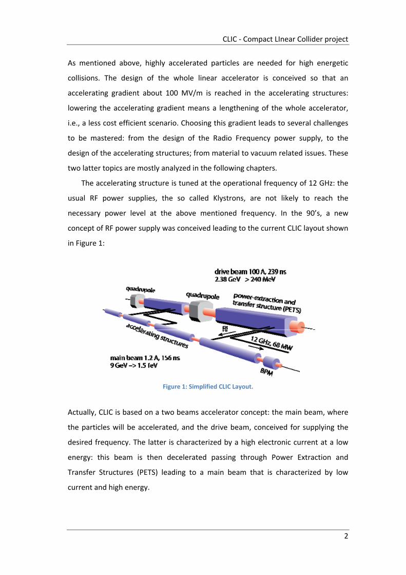
The accelerating structure is tuned at the operational frequency of 12 GHz: the
usual RF power supplies, the so called Klystrons, are not likely to reach the
necessary power level at the above mentioned frequency. In the 90’s, a new
concept of RF power supply was conceived leading to the current CLIC layout shown
in Figure 1:
Figure 1: Simplified CLIC Layout.
Actually, CLIC is based on a two beams accelerator concept: the main beam, where
the particles will be accelerated, and the drive beam, conceived for supplying the
desired frequency. The latter is characterized by a high electronic current at a low
energy: this beam is then decelerated passing through Power Extraction and
Transfer Structures (PETS) leading to a main beam that is characterized by low
current and high energy.
CLIC ‐ Compact LInear Collider project
3
From the accelerating structures point of view, aiming at reaching the above
mentioned accelerating gradient, these are designed as travelling wave structures
instead of standing wave accelerating structures that are not likely to accomplish
the accelerating function. In addition, these structures are conceived to work at
room temperature: the cryogenic technology leading to superconductive structures
can’t be used at this gradient.
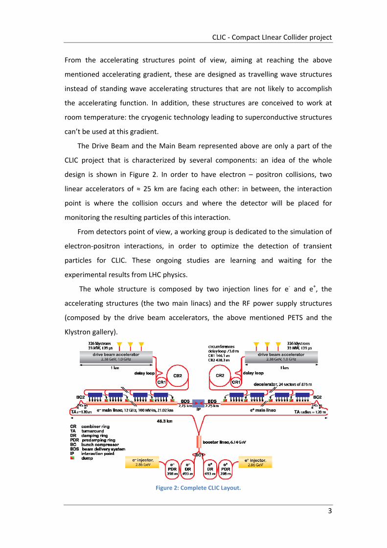
The Drive Beam and the Main Beam represented above are only a part of the
CLIC project that is characterized by several components: an idea of the whole
design is shown in Figure 2. In order to have electron – positron collisions, two
linear accelerators of ≈ 25 km are facing each other: in between, the interaction
point is where the collision occurs and where the detector will be placed for
monitoring the resulting particles of this interaction.
From detectors point of view, a working group is dedicated to the simulation of
electron‐positron interactions, in order to optimize the detection of transient
particles for CLIC. These ongoing studies are learning and waiting for the
experimental results from LHC physics.
The whole structure is composed by two injection lines for e‐ and e+, the
accelerating structures (the two main linacs) and the RF power supply structures
(composed by the drive beam accelerators, the above mentioned PETS and the
Klystron gallery).
Figure 2: Complete CLIC Layout.
CLIC ‐ Compact LInear Collider project
4
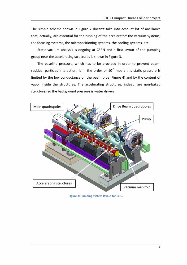
The simple scheme shown in Figure 2 doesn’t take into account lot of ancillaries
that, actually, are essential for the running of the accelerator: the vacuum systems,
the focusing systems, the micropositioning systems, the cooling systems, etc.
Static vacuum analysis is ongoing at CERN and a first layout of the pumping
group near the accelerating structures is shown in Figure 3.
The baseline pressure, which has to be provided in order to prevent beam‐
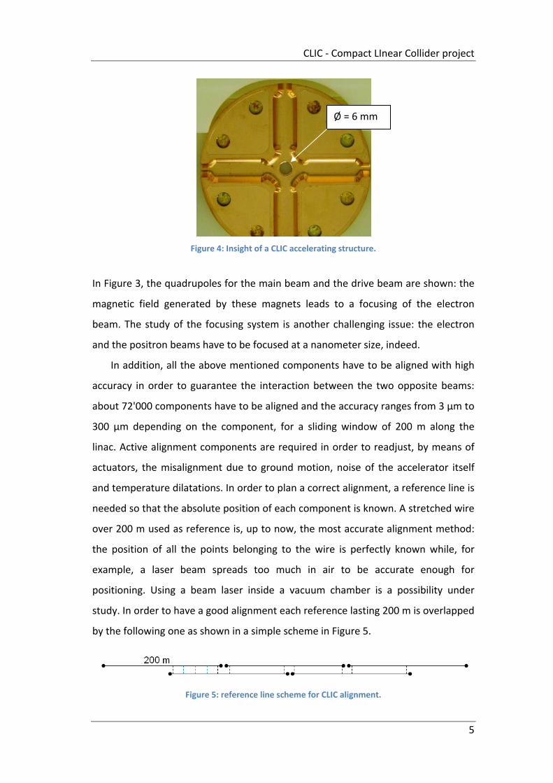
residual particles interaction, is in the order of 10‐9 mbar: this static pressure is
limited by the low conductance on the beam pipe (Figure 4) and by the content of
vapor inside the structures. The accelerating structures, indeed, are non‐baked
structures so the background pressure is water driven.
Figure 3: Pumping System layout for CLIC.
Pump
Main quadrupoles Drive Beam quadrupoles
Vacuum manifold Accelerating structures
CLIC ‐ Compact LInear Collider project
5
Figure 4: Insight of a CLIC accelerating structure.
In Figure 3, the quadrupoles for the main beam and the drive beam are shown: the
magnetic field generated by these magnets leads to a focusing of the electron
beam. The study of the focusing system is another challenging issue: the electron
and the positron beams have to be focused at a nanometer size, indeed.
In addition, all the above mentioned components have to be aligned with high
accuracy in order to guarantee the interaction between the two opposite beams:
about 72'000 components have to be aligned and the accuracy ranges from 3 μm to
300 μm depending on the component, for a sliding window of 200 m along the
linac. Active alignment components are required in order to readjust, by means of
actuators, the misalignment due to ground motion, noise of the accelerator itself
and temperature dilatations. In order to plan a correct alignment, a reference line is
needed so that the absolute position of each component is known. A stretched wire
over 200 m used as reference is, up to now, the most accurate alignment method:
the position of all the points belonging to the wire is perfectly known while, for
example, a laser beam spreads too much in air to be accurate enough for
positioning. Using a beam laser inside a vacuum chamber is a possibility under
study. In order to have a good alignment each reference lasting 200 m is overlapped
by the following one as shown in a simple scheme in Figure 5.
Figure 5: reference line scheme for CLIC alignment.
Ø = 6 mm
CLIC ‐ Compact LInear Collider project
6
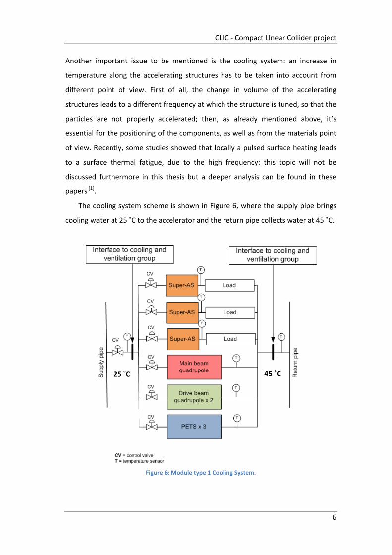
Another important issue to be mentioned is the cooling system: an increase in
temperature along the accelerating structures has to be taken into account from
different point of view. First of all, the change in volume of the accelerating
structures leads to a different frequency at which the structure is tuned, so that the
particles are not properly accelerated; then, as already mentioned above, it’s
essential for the positioning of the components, as well as from the materials point
of view. Recently, some studies showed that locally a pulsed surface heating leads
to a surface thermal fatigue, due to the high frequency: this topic will not be
discussed furthermore in this thesis but a deeper analysis can be found in these
papers [1].
The cooling system scheme is shown in Figure 6, where the supply pipe brings
cooling water at 25 ˚C to the accelerator and the return pipe collects water at 45 ˚C.
Figure 6: Module type 1 Cooling System.
25 ˚C 45 ˚C
CLIC ‐ Compact LInear Collider project
7
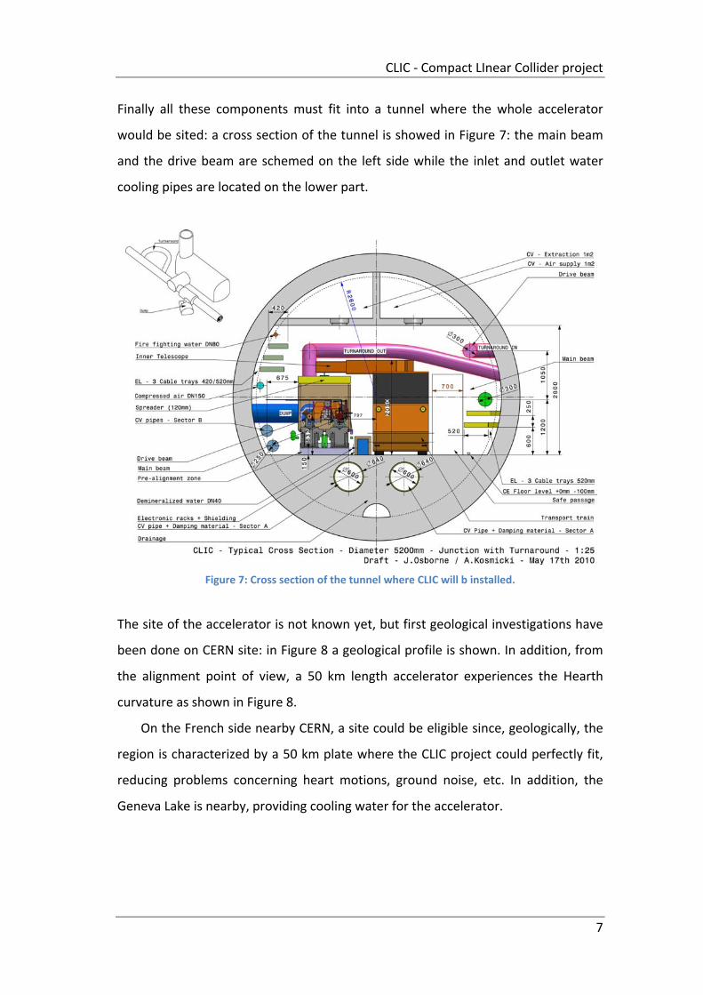
Finally all these components must fit into a tunnel where the whole accelerator
would be sited: a cross section of the tunnel is showed in Figure 7: the main beam
and the drive beam are schemed on the left side while the inlet and outlet water
cooling pipes are located on the lower part.
Figure 7: Cross section of the tunnel where CLIC will b installed.
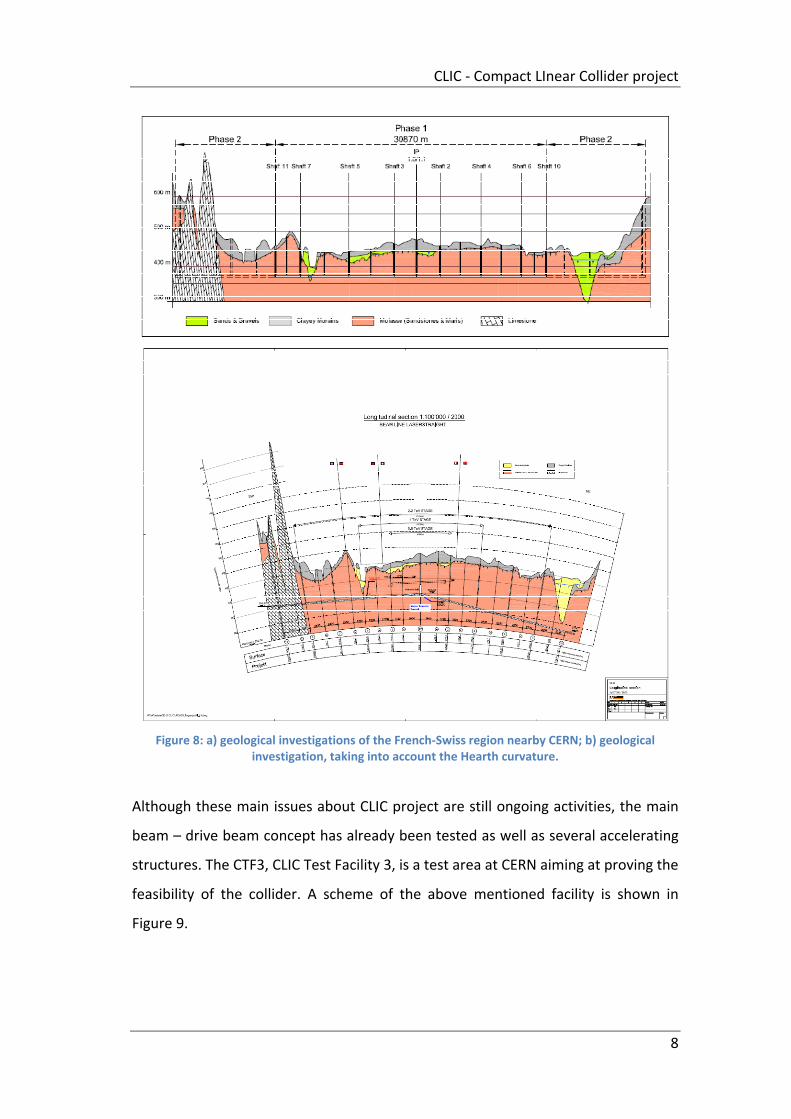
The site of the accelerator is not known yet, but first geological investigations have
been done on CERN site: in Figure 8 a geological profile is shown. In addition, from
the alignment point of view, a 50 km length accelerator experiences the Hearth
curvature as shown in Figure 8.
On the French side nearby CERN, a site could be eligible since, geologically, the
region is characterized by a 50 km plate where the CLIC project could perfectly fit,
reducing problems concerning heart motions, ground noise, etc. In addition, the
Geneva Lake is nearby, providing cooling water for the accelerator.
CLIC ‐ Compact LInear Collider project
8
Figure 8: a) geological investigations of the French‐Swiss region nearby CERN; b) geological investigation, taking into account the Hearth curvature.
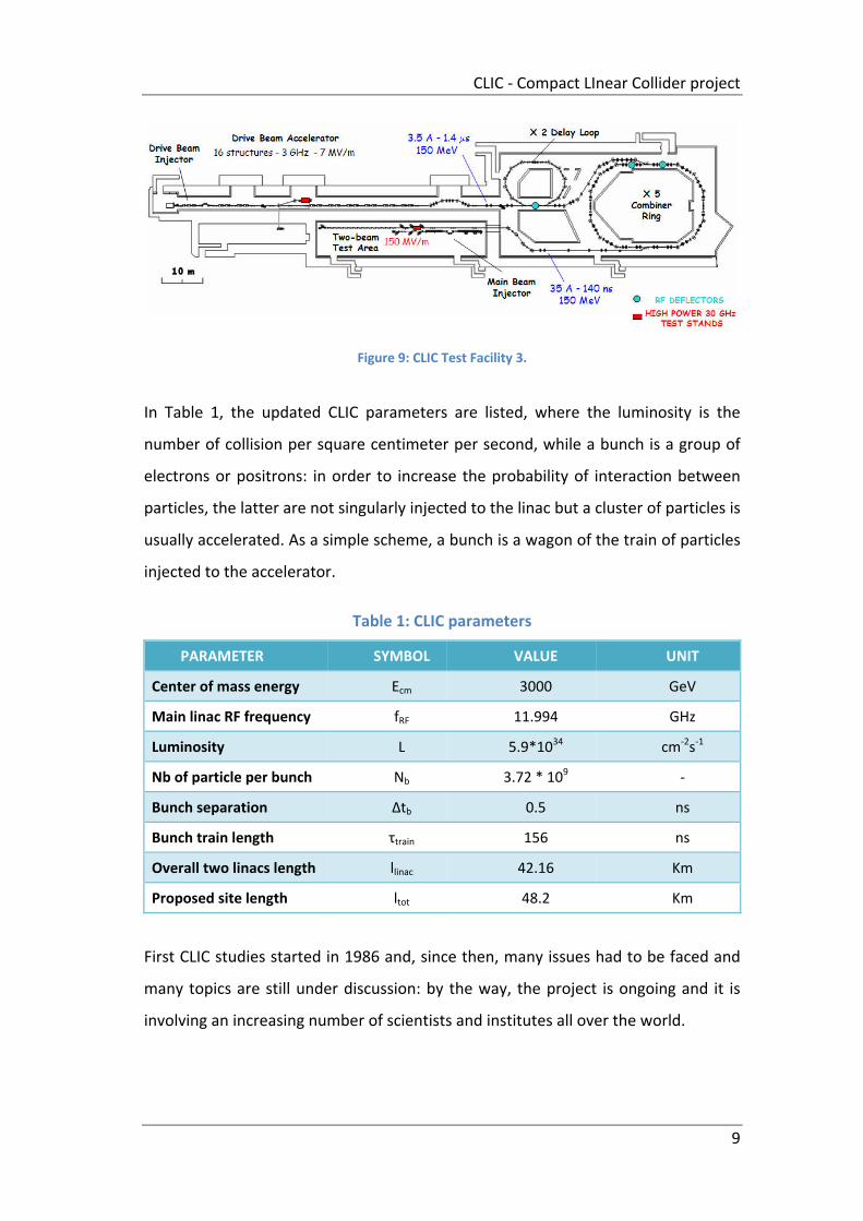
Although these main issues about CLIC project are still ongoing activities, the main
beam – drive beam concept has already been tested as well as several accelerating
structures. The CTF3, CLIC Test Facility 3, is a test area at CERN aiming at proving the
feasibility of the collider. A scheme of the above mentioned facility is shown in
Figure 9.
CLIC ‐ Compact LInear Collider project
9
Figure 9: CLIC Test Facility 3.
In Table 1, the updated CLIC parameters are listed, where the luminosity is the
number of collision per square centimeter per second, while a bunch is a group of
electrons or positrons: in order to increase the probability of interaction between
particles, the latter are not singularly injected to the linac but a cluster of particles is
usually accelerated. As a simple scheme, a bunch is a wagon of the train of particles
injected to the accelerator.
Table 1: CLIC parameters
PARAMETER SYMBOL VALUE UNIT
Center of mass energy Ecm 3000 GeV
Main linac RF frequency fRF 11.994 GHz
Luminosity L 5.9*1034 cm‐2s‐1
Nb of particle per bunch Nb 3.72 * 109 ‐
Bunch separation Δtb 0.5 ns
Bunch train length τtrain 156 ns
Overall two linacs length llinac 42.16 Km
Proposed site length ltot 48.2 Km
First CLIC studies started in 1986 and, since then, many issues had to be faced and
many topics are still under discussion: by the way, the project is ongoing and it is
involving an increasing number of scientists and institutes all over the world.
Dynamic Vacuum: an Issue for CLIC Accelerating Structures
10
CHAPTER 2
DYNAMIC VACUUM: AN ISSUE FOR CLIC
ACCELERATING STRUCTURES
Vacuum requirements for accelerators technology are strongly related to the need
of reducing the beam‐residual molecules interaction, in order to prevent the beam
instability. For a correct design, it’s necessary, indeed, to take into account not only
the static background pressure but also the dynamic effects due to the high
gradient condition at which the accelerator is running.
The vacuum analysis of CLIC accelerating structures has several constraints
allowing a baseline pressure of ~ 10‐9 mbar. First of all, the bore hole, where the
beam line is passing through, has a diameter of ~ 6 mm, so that the pumping speed
of each gas species is limited by the geometry of the accelerating structures. Then,
the accelerating structures are supposed not to be baked, a typical procedure for
any vacuum system: heating up all the vacuum chambers and the pumping groups
to higher temperatures, ranging from 100°C to 250°C, the water sojourn time is
sensitively reduced (see paragraph 4.5). This procedure allows reaching a lower
baseline pressure in lower time. Furthermore, the high accelerating gradient (~100
MV/m) induces breakdowns inside the structures leading to local bursts of pressure:
actually, vacuum sparks release locally a huge amount of energy creating craters on
the surface. Finally, field emitted dark currents, easily induced by the above
mentioned high electric field, impinge on the inner walls of the structure causing
Dynamic Vacuum: an Issue for CLIC Accelerating Structures
11
the electron stimulated desorption effect, the main topic which this thesis is
focused on.
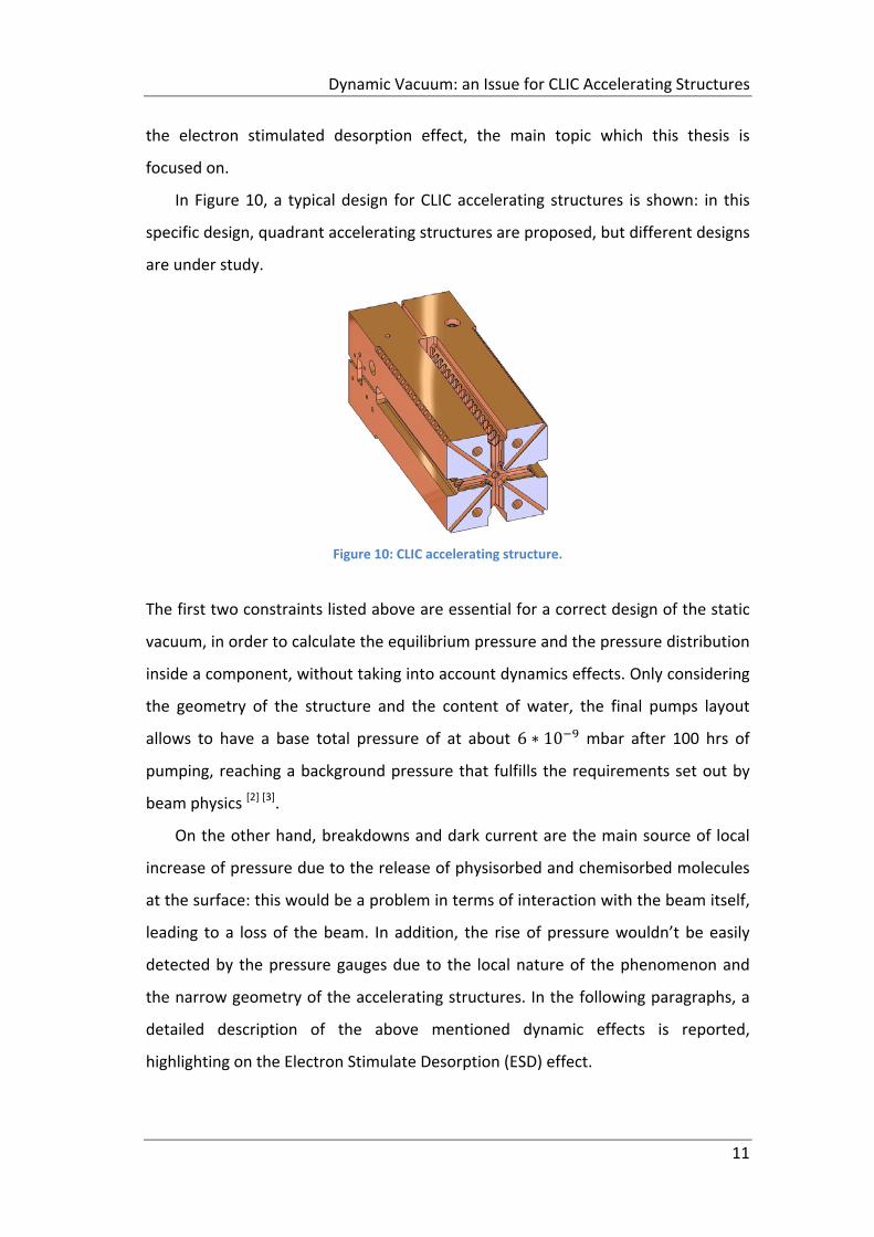
In Figure 10, a typical design for CLIC accelerating structures is shown: in this
specific design, quadrant accelerating structures are proposed, but different designs
are under study.
Figure 10: CLIC accelerating structure.
The first two constraints listed above are essential for a correct design of the static
vacuum, in order to calculate the equilibrium pressure and the pressure distribution
inside a component, without taking into account dynamics effects. Only considering
the geometry of the structure and the content of water, the final pumps layout
allows to have a base total pressure of at about 6 ∗ 10 mbar after 100 hrs of
pumping, reaching a background pressure that fulfills the requirements set out by
beam physics [2] [3].
On the other hand, breakdowns and dark current are the main source of local
increase of pressure due to the release of physisorbed and chemisorbed molecules
at the surface: this would be a problem in terms of interaction with the beam itself,
leading to a loss of the beam. In addition, the rise of pressure wouldn’t be easily
detected by the pressure gauges due to the local nature of the phenomenon and
the narrow geometry of the accelerating structures. In the following paragraphs, a
detailed description of the above mentioned dynamic effects is reported,
highlighting on the Electron Stimulate Desorption (ESD) effect.
Dynamic Vacuum: an Issue for CLIC Accelerating Structures
12
2.1 Dynamic Vacuum Sources: Breakdowns and Dark Currents
Concerning the dynamic vacuum, there are two are main sources of local bursts of
pressure: breakdowns, i.e. vacuum sparks, and dark currents, i.e. field‐emitted
electrons. Both of these phenomena are triggered by the high electric field
characterizing CLIC accelerating structures.
2.1.1 Breakdowns Studies
Since 2000, breakdowns studies are ongoing at CERN, aiming at understanding the
behavior of different materials under high electric field, in order to reach a
threshold of 10‐7 breakdown rate in the accelerating structures.
From a theoretical point of view , a 1‐D and 2‐D Particle‐In‐Cell code have been
developed by Dr. H. Timko and collaborators from Physics Helsinki University
describing the characteristics of the plasma between an anode and a cathode,
inside a vacuum chamber where a high electric field is applied. These two codes
successfully describe the plasma build up, based on the hypothesis that there are
field emitters (tips, peaks with higher roughness…) on the surface of the material,
enhancing the electric field locally so that electrons are field emitted from the
cathode. This current flowing into the tips leads to a local heating that allows the
evaporation of metallic neutrals: the ionization of these neutrals is due, then, to the
interaction with electrons. Ions are so energetic that, accelerated toward the
surface of the cathode, they melt the surface; this bombardment leads to the
release of metallic neutrals from the surface, sustaining the arcing process. In an RF
accelerating structure, the role of the cathode and the anode are continuously
switched, so that the entire accelerating structure surface acts as a cathode and as
an anode almost at the same time.
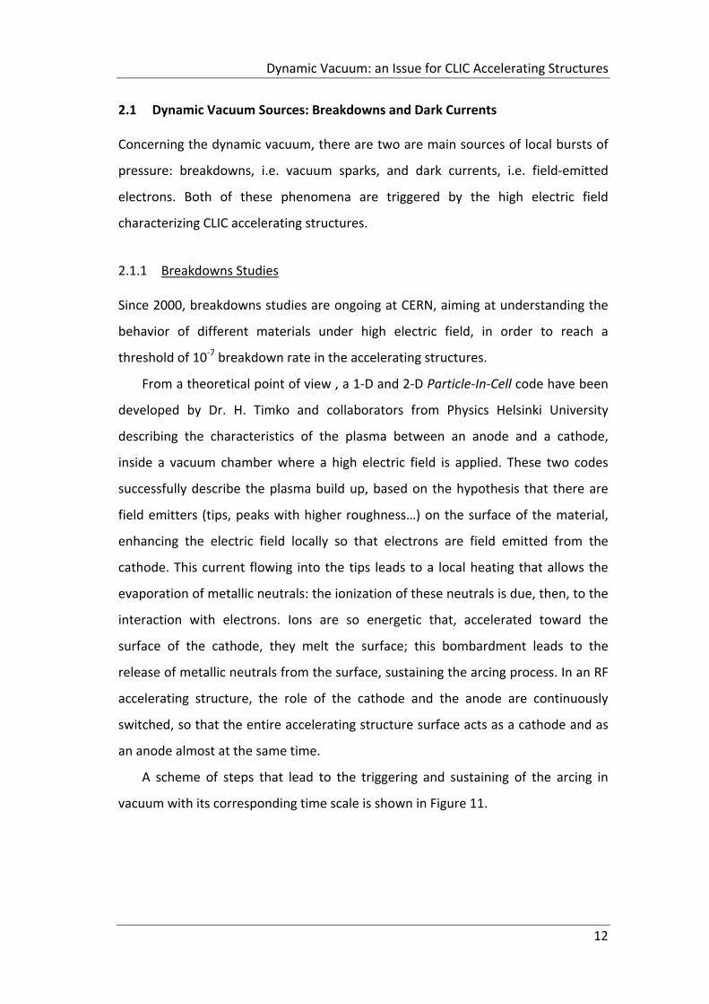
A scheme of steps that lead to the triggering and sustaining of the arcing in
vacuum with its corresponding time scale is shown in Figure 11.
Dynamic Vacuum: an Issue for CLIC Accelerating Structures
13
Figure 11: Triggering and sustaining of the arcing in vacuum.
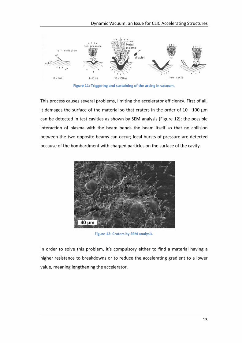
This process causes several problems, limiting the accelerator efficiency. First of all,
it damages the surface of the material so that craters in the order of 10 ‐ 100 µm
can be detected in test cavities as shown by SEM analysis (Figure 12); the possible
interaction of plasma with the beam bends the beam itself so that no collision
between the two opposite beams can occur; local bursts of pressure are detected
because of the bombardment with charged particles on the surface of the cavity.
Figure 12: Craters by SEM analysis.
In order to solve this problem, it’s compulsory either to find a material having a
higher resistance to breakdowns or to reduce the accelerating gradient to a lower
value, meaning lengthening the accelerator.
Dynamic Vacuum: an Issue for CLIC Accelerating Structures
14
2.1.2 Experimental Set‐up and Results
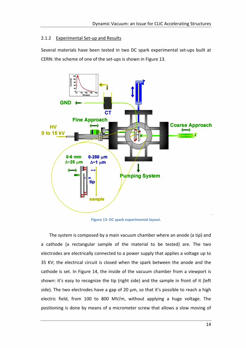
Several materials have been tested in two DC spark experimental set‐ups built at
CERN: the scheme of one of the set‐ups is shown in Figure 13.
Figure 13: DC spark experimental layout.
The system is composed by a main vacuum chamber where an anode (a tip) and
a cathode (a rectangular sample of the material to be tested) are. The two
electrodes are electrically connected to a power supply that applies a voltage up to
35 KV; the electrical circuit is closed when the spark between the anode and the
cathode is set. In Figure 14, the inside of the vacuum chamber from a viewport is
shown: it’s easy to recognize the tip (right side) and the sample in front of it (left
side). The two electrodes have a gap of 20 µm, so that it’s possible to reach a high
electric field, from 100 to 800 MV/m, without applying a huge voltage. The
positioning is done by means of a micrometer screw that allows a slow moving of
Dynamic Vacuum: an Issue for CLIC Accelerating Structures
15
the tip toward the sample: once the anode and the cathode are in contact, so the
zero of the gap is set, the tip is moved backward reaching the desired gap.
Figure 14: Vacuum chamber from a viewport.
The system can run in three different modes: field emission mode, the green path
where the Switch3 is closed in the electric circuit (Figure 15); the saturated field ;
the Breakdown Rate. Both saturated field and the Breakdown Rate modes are
characterized by the same electrical path by closing S1 and S2 (blue arrows). In FE
mode, currents in the order of the pA are measured and the field enhancement
factor β can be calculated from the Fowler‐Nordheim law describing the field
emitted currents as [4]:
1.54 ∗ 10 ∗
exp 10.41 exp6.53 ∗ 10 φ /
βE Eq. 1
where is the current density / , is the electric field / , is the
work function, . The fit of β is done in a linear regime from 2*10‐11 to 10‐9 A.
Dynamic Vacuum: an Issue for CLIC Accelerating Structures
16
Figure 15: Spark system electrical circuit.
The field enhancement factor is directly realted to the local electric field :
Eq. 2
Therefore, because of protrusions at the surface of the sample, the electric field is
locally enhanced (~10 GV/m) and leads to the tunneling of electrons causing a local
heating up of the surface. In the FE mode, the starting point of the setting of the
plasma is monitored.
In order to have parameters through which compare different materials and
surface treatments the run into BF and BDR mode is needed.
The first one defines the external electric field at which breakdowns occur: the
measurement run by raising up the voltage, so the external electric field. The
measured current is in the order of 100 A during a spark. A typical curve is shown in
Figure 16: different materials show a conditioning or de‐conditioning behavior
before reaching the saturated field. For example, Mo shows a conditioning phase
lasting 60‐70 breakdowns, while Cu after 20 breakdowns is completely conditioned.
Experiments on oxidized Cu showed a de‐conditioning phase lasting 20‐40
breakdowns.
50 MΩ
25 ΩS1 S2
S3
HV 0‐12 KV
Tip
Sample
UHV
x z
y
1 MΩ
C To
27 nF 1 nF
FE
Eb and BDR path
FE
Eb and BDR path
HV
Probe
(
A Electrometer
Out Measure
I t
In
Dynamic Vacuum: an Issue for CLIC Accelerating Structures
17
(a) (b) (c)
Figure 16: Condition and de‐conditioning of several materials: a) Molybdenum; b) Copper and c) Oxidized Copper.
Comparing these materials leads to several conclusions: it’s easier to ‘clean’ by
means of few sparks a copper surface instead of a molybdenum one; Mo shows a
better breakdown ‘resistance’ than Cu because its saturated field is much higher.
Despite this, copper, having a saturated field of 200 MV/m, is still the main
candidate for CLIC because of its electrical conductivity.
As previously said, several materials have been tested and the corresponding
ranking is shown in Figure 17. This ranking highlights the relationship between the
lattice structure of materials and the saturated field. The HCP materials have a
higher saturated breakdown field: this suggests that the motion of dislocations
inside the material could be a phenomenon that contributes to the triggering of a
breakdown.
Molecular Dynamics simulations, performed by Dr. F. Djurabekova et alii, show
that the motion of dislocations inside the material can bring to voids that, pulled by
the external electric field, build the protrusions at the surface igniting the
breakdown. In order to validate this new theory, measurements of the breakdown
field at different temperatures are planned.
The second parameter listed above is the Breakdown Rate that measures the
numbers of breakdowns over the number of attempts. The measurement in this
case is done at a desired voltage that is continuously applied until a breakdown is
registered. A typical curve is shown in Figure 18.
Cu2O
Dynamic Vacuum: an Issue for CLIC Accelerating Structures
18
Figure 17: Ranking of tested materials: dependence on the crystallographic structure.
Figure 18: Breakdown Rate and β measurements.
The aim of this measurement is to determine at which accelerating field the
structure can be run so that the BDR is lower than a threshold value that is
estimated to be around 10‐7.
Every time that the field reaches a zero value, a breakdown is registered:
typically there are bunches of breakdowns separated by ‘quiet periods’ where the
field enhancement factor increases. During these periods it seems that the surface
is in evolution until another breakdown occurs.
125
100
75
50
25
0
225 MV/m
β
Nb of Attempts
250
200
150
100
50
0
Field [M
V/m
]
Dynamic Vacuum: an Issue for CLIC Accelerating Structures
19
Finally, It’s important to underline that a full comparison between RF sparks and DC
sparks can’t be done because the two experiments differ a lot: in RF structures the
whole cavity is conditioned while in the DC spark set‐up only a little spot is tested;
in RF cavities the BDR depends not only on the material but also on the pulse length
and on the repetition rate. By the way the DC set‐up it’s a rather simple and cheap
system where several materials, characterized by different surface treatments, can
be tested in function of voltage, energy and temperature.
From the dynamic vacuum point of view, some measurements have been done
in the past by means of a Residual Gas Analyzer: this instrument allows the scanning
of different masses giving the composition of the vacuum inside the chamber (a
precise description of the instrument will be provided in chapter 4). As previously
underlined, a gas burst always follows a breakdown: considering the number of
molecules released during a spark, it’s possible to calculate if this can be dangerous
for the beam or not.
2.1.3 Breakdown Dynamic Vacuum Simulations
The dynamic vacuum threshold for preventing fast ion beam instability is so that the
partial pressures of CO2 and H2 must be lower than 10‐9 Torr. Considering this limit
value, simulations have been performed recently at CERN [3].
In order to determine the pressure profile along the accelerating structures, a
time dependent behavior of the gas has been simulated with two different
methods: the first one is based on a Monte Carlo algorithm implemented in a finite
element code; the second one uses the vacuum ‐ thermal analogy where thermal
simulations have been analyzed.
The Monte Carlo simulation is based on the principle that every gas molecule
must be tracked in time within a volume that, in the specific case of CLIC
accelerating structures, is the cavity where the electronic beam is supposed to pass
through. The particles to be tracked are generated in different parts of the cavity:
inside the volume, in order to take into account the initial volume pressure; over
Dynamic Vacuum: an Issue for CLIC Accelerating Structures
20
the inner surface of the cavity for simulating the out‐gassing of copper; locally,
because of breakdowns.
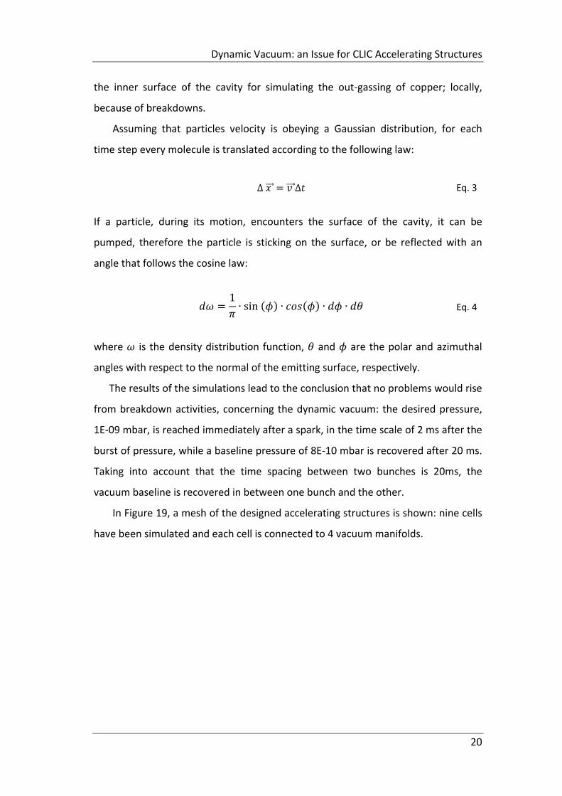
Assuming that particles velocity is obeying a Gaussian distribution, for each
time step every molecule is translated according to the following law:
∆ ∆ Eq. 3
If a particle, during its motion, encounters the surface of the cavity, it can be
pumped, therefore the particle is sticking on the surface, or be reflected with an
angle that follows the cosine law:
1∙ sin ∙ ∙ ∙ Eq. 4
where is the density distribution function, and are the polar and azimuthal
angles with respect to the normal of the emitting surface, respectively.
The results of the simulations lead to the conclusion that no problems would rise
from breakdown activities, concerning the dynamic vacuum: the desired pressure,
1E‐09 mbar, is reached immediately after a spark, in the time scale of 2 ms after the
burst of pressure, while a baseline pressure of 8E‐10 mbar is recovered after 20 ms.
Taking into account that the time spacing between two bunches is 20ms, the
vacuum baseline is recovered in between one bunch and the other.
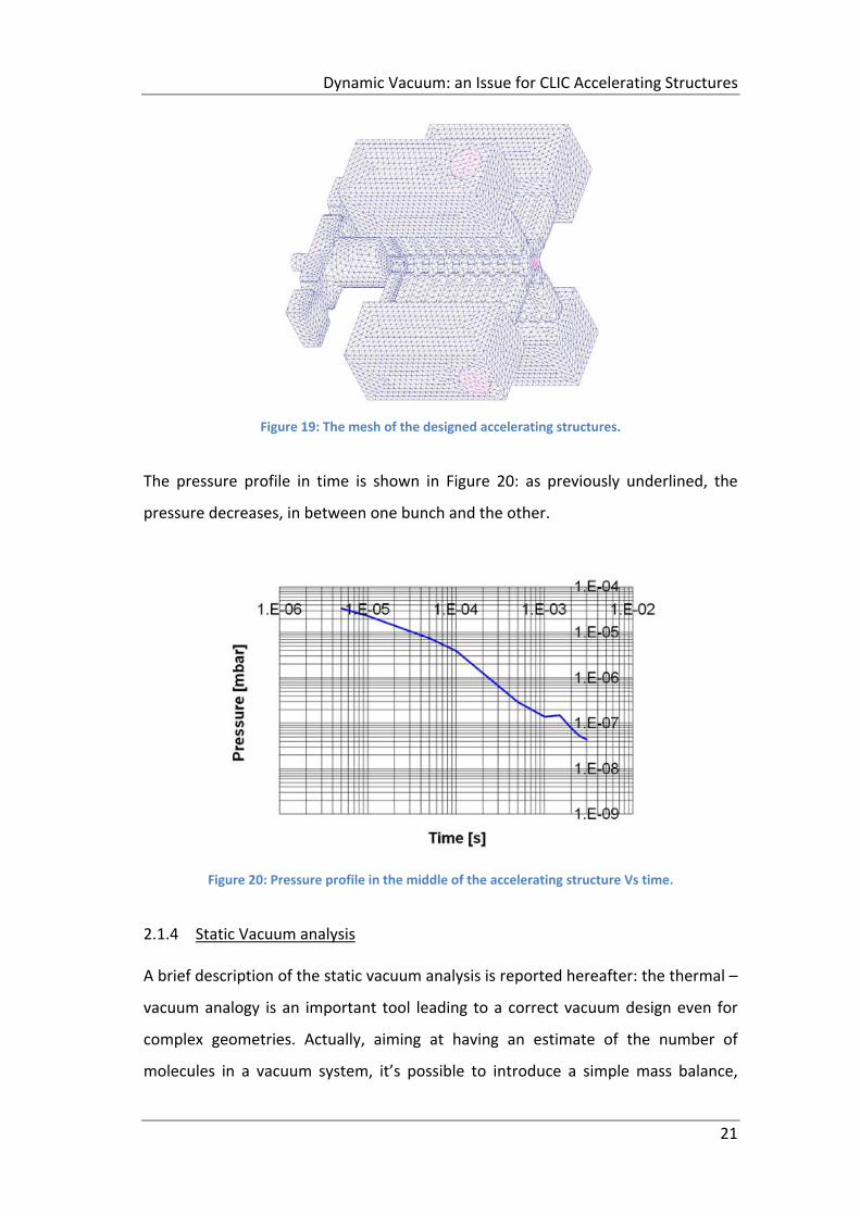
In Figure 19, a mesh of the designed accelerating structures is shown: nine cells
have been simulated and each cell is connected to 4 vacuum manifolds.
Dynamic Vacuum: an Issue for CLIC Accelerating Structures
21
Figure 19: The mesh of the designed accelerating structures.
The pressure profile in time is shown in Figure 20: as previously underlined, the
pressure decreases, in between one bunch and the other.
Figure 20: Pressure profile in the middle of the accelerating structure Vs time.
2.1.4 Static Vacuum analysis
A brief description of the static vacuum analysis is reported hereafter: the thermal –
vacuum analogy is an important tool leading to a correct vacuum design even for
complex geometries. Actually, aiming at having an estimate of the number of
molecules in a vacuum system, it’s possible to introduce a simple mass balance,
Dynamic Vacuum: an Issue for CLIC Accelerating Structures
22
taking into account the outgassing rate of the surfaces, the molecules in a certain
volume and the pumping speed of the system. This 1 –D approach could be simple if
the geometry of the system is simple as well, while in most of cases is not.
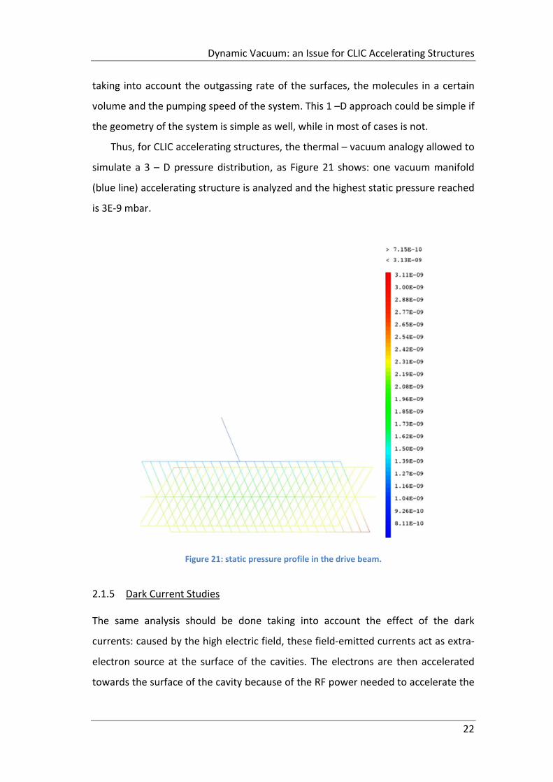
Thus, for CLIC accelerating structures, the thermal – vacuum analogy allowed to
simulate a 3 – D pressure distribution, as Figure 21 shows: one vacuum manifold
(blue line) accelerating structure is analyzed and the highest static pressure reached
is 3E‐9 mbar.
Figure 21: static pressure profile in the drive beam.
2.1.5 Dark Current Studies
The same analysis should be done taking into account the effect of the dark
currents: caused by the high electric field, these field‐emitted currents act as extra‐
electron source at the surface of the cavities. The electrons are then accelerated
towards the surface of the cavity because of the RF power needed to accelerate the
Dynamic Vacuum: an Issue for CLIC Accelerating Structures
23
beam. Impinging on the surface, the adsorbed particles are released leading to a
local burst of pressure (Electron Stimulated Desorption effect).
In order to evaluate if the local increase of pressure could be a real problem for
the beam life, an estimate has been done by S. Calatroni, by means of experimental
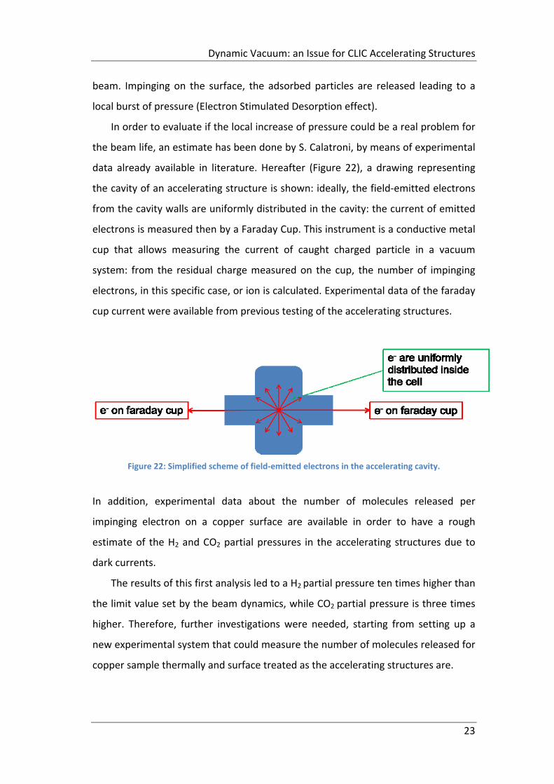
data already available in literature. Hereafter (Figure 22), a drawing representing
the cavity of an accelerating structure is shown: ideally, the field‐emitted electrons
from the cavity walls are uniformly distributed in the cavity: the current of emitted
electrons is measured then by a Faraday Cup. This instrument is a conductive metal
cup that allows measuring the current of caught charged particle in a vacuum
system: from the residual charge measured on the cup, the number of impinging
electrons, in this specific case, or ion is calculated. Experimental data of the faraday
cup current were available from previous testing of the accelerating structures.
Figure 22: Simplified scheme of field‐emitted electrons in the accelerating cavity.
In addition, experimental data about the number of molecules released per
impinging electron on a copper surface are available in order to have a rough
estimate of the H2 and CO2 partial pressures in the accelerating structures due to
dark currents.
The results of this first analysis led to a H2 partial pressure ten times higher than
the limit value set by the beam dynamics, while CO2 partial pressure is three times
higher. Therefore, further investigations were needed, starting from setting up a
new experimental system that could measure the number of molecules released for
copper sample thermally and surface treated as the accelerating structures are.
Dynamic Vacuum: an Issue for CLIC Accelerating Structures
24
A detailed description of the copper samples and the experimental set‐up are
the main topics of the following chapters, while the paragraph hereafter is going to
describe the theoretical models behind the Electron Stimulated Desorption (ESD)
effect.
2.2 Electron Stimulated Desorption: fundamental mechanisms
Energetic particles (e‐, H+ , He+, hν) may cause desorption and fragmentation at
surfaces by inducing electronic transitions to dissociative states. Studying these
processes is an important area in surface chemistry and physics, with many
implications in basic science and technology. Such a process involves the nature of
chemical bonding at surfaces in both the ground and excited states, surface
dynamical processes involving charge or energy transfer, interactions among
adsorbates, and the conversion of electronic potential energy into nuclear motion.
Desorption induced by electronic transitions (DIET) is widely encountered in nature
and in laboratories. For example, the surfaces of materials in the solar system and
the interstellar media are exposed to energetic photons and particles that stimulate
desorption processes. In vacuum laboratories, DIET processes occur in almost every
system involving the impact of energetic photons or charged particles on solid
surfaces.
The processes of stimulated desorption and fragmentation have some unique
characteristics that make them valuable for a variety of applications. For example,
one can provide non thermal energy to control surface reactions with very high
spatial resolution by using focused electron or photon beams. The research area on
materials growth, modification, and patterning with these methods is very active.
DIET processes must also be controlled and considered in electron microscopy and
in surface analytical techniques such as photo‐emission, Auger and electron‐energy‐
Ioss spectroscopies, low‐energy electron diffraction, etc. In this case, desorption or
fragmentation may be an unwanted side effect caused by probing the surface with
photons or electrons. On a more macroscopic scale, DIET processes play a role in
Dynamic Vacuum: an Issue for CLIC Accelerating Structures
25
plasma‐wall interactions, in the operation of synchrotrons, and more generally in
the stability of materials subjected to various forms of radiation.
This thesis will be focused on basic mechanisms of desorption at surfaces:
different models and hypothesis has been made in order to clarify what happens to
the adsorbates during the ‘bombardment’ of the surface and a short review will be
presented in the following paragraphs.
2.2.1 The Menzel‐Gomer‐Redhead Model
The MGR model [16] [17] was conceived in order to understand why electronically‐
induced dissociation processes on surfaces proceed differently in comparison to
similar species in the gas phase. This model describes the behavior of an adsorbate
when energetic particles, for example electrons, bombard it. The desorbed species
can be either neutrals or ions: several different desorption sequences are possible.
However, it’s not the aim of this model quantifying which one is the most probable
channel leading to the desorption of a specie.
As a starting point of the model, the direct momentum transferred to an
adsorbate by an energetic electron is negligible so an electronic excitation is
required in order to describe the dissociation of atoms or molecules from the
surface.
The model is a two‐steps mechanism. The first one is a Franck‐Condon
transition: electronic transitions are essentially instantaneous compared with the
time scale of nuclear motions. Therefore, if the molecule has to move to a new
vibrational level during the electronic transition, it will move to a favored one, i.e.,
the one allowing the minimal change in the nuclear coordinates.
The second step is characterized by a quenching or delocalization of the
excitation that leads to a recapture or to a leaving (neutral or ionic) particle, and/or
to reneutralization of a leaving ion. This second step has a longer timescale than the
first one; desorption takes place when the total energy of the adparticle is higher
than the binding energy.
Dynamic Vacuum: an Issue for CLIC Accelerating Structures
26
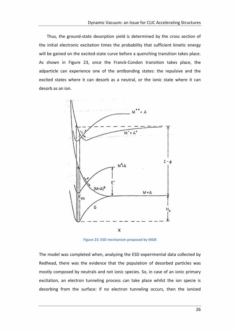
Thus, the ground‐state desorption yield is determined by the cross section of
the initial electronic excitation times the probability that sufficient kinetic energy
will be gained on the excited‐state curve before a quenching transition takes place.
As shown in Figure 23, once the Franck‐Condon transition takes place, the
adparticle can experience one of the antibonding states: the repulsive and the
excited states where it can desorb as a neutral, or the ionic state where it can
desorb as an ion.
Figure 23: ESD mechanism proposed by MGR
The model was completed when, analyzing the ESD experimental data collected by
Redhead, there was the evidence that the population of desorbed particles was
mostly composed by neutrals and not ionic species. So, in case of an ionic primary
excitation, an electron tunneling process can take place whilst the ion specie is
desorbing from the surface: if no electron tunneling occurs, then the ionized
Dynamic Vacuum: an Issue for CLIC Accelerating Structures
27
adparticle can desorb; otherwise the excited particle is quenched and it can be
recaptured (no desorption takes place), or desorbed as a neutral. Adding this new
part of the model, it was possible to describe the different paths that the adsorbate
experiences during the desorption process.
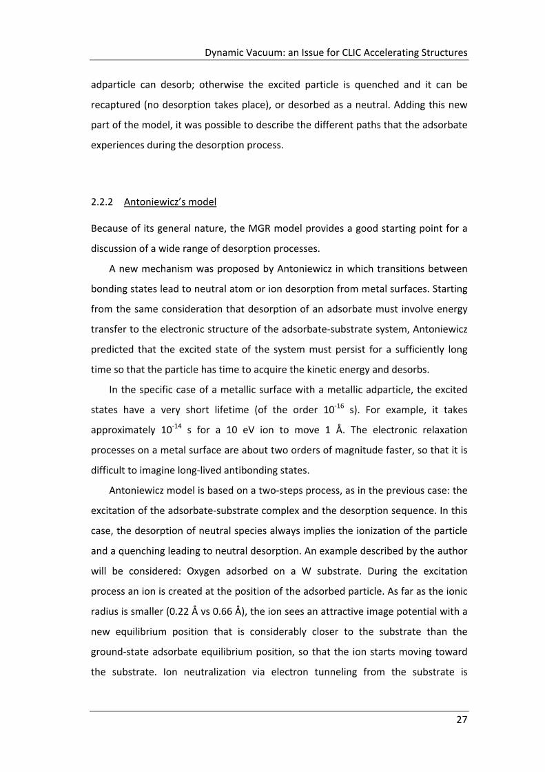
2.2.2 Antoniewicz’s model
Because of its general nature, the MGR model provides a good starting point for a
discussion of a wide range of desorption processes.
A new mechanism was proposed by Antoniewicz in which transitions between
bonding states lead to neutral atom or ion desorption from metal surfaces. Starting
from the same consideration that desorption of an adsorbate must involve energy
transfer to the electronic structure of the adsorbate‐substrate system, Antoniewicz
predicted that the excited state of the system must persist for a sufficiently long
time so that the particle has time to acquire the kinetic energy and desorbs.
In the specific case of a metallic surface with a metallic adparticle, the excited
states have a very short lifetime (of the order 10‐16 s). For example, it takes
approximately 10‐14 s for a 10 eV ion to move 1 Å. The electronic relaxation
processes on a metal surface are about two orders of magnitude faster, so that it is
difficult to imagine long‐lived antibonding states.
Antoniewicz model is based on a two‐steps process, as in the previous case: the
excitation of the adsorbate‐substrate complex and the desorption sequence. In this
case, the desorption of neutral species always implies the ionization of the particle
and a quenching leading to neutral desorption. An example described by the author
will be considered: Oxygen adsorbed on a W substrate. During the excitation
process an ion is created at the position of the adsorbed particle. As far as the ionic
radius is smaller (0.22 Å vs 0.66 Å), the ion sees an attractive image potential with a
new equilibrium position that is considerably closer to the substrate than the
ground‐state adsorbate equilibrium position, so that the ion starts moving toward
the substrate. Ion neutralization via electron tunneling from the substrate is
Dynamic Vacuum: an Issue for CLIC Accelerating Structures
28
represented by a vertical jump from the upper to the lower potential curve (see
Figure 24): the kinetic energy that the ion had at the time of the neutralization is
unchanged so that the total energy of the neutral is the kinetic energy before
neutralization plus the potential energy of the lower curve at the position of the
neutralization.
Figure 24: Antoniewicz’s ESD model for neutrals desorption.
The crossing of the neutral and ion potential‐energy curves represents the crossing
of the Fermi level by the atomic energy level, reversing the direction of allowed
electron tunneling.
If the sum of the two energies is greater than the binding energy, the neutral
desorbs, i.e. :
≡ 0 Eq. 5
Where is the potential curve describing the excited state, while is the ground
potential curve. If 0 then the particle remains trapped at the surface with
the surface bond excited. The inequality described in Eq. 5 implies that the distance
Dynamic Vacuum: an Issue for CLIC Accelerating Structures
29
∆ | | travelled by the ion before reneutralization must be larger than
certain critical distance ∆ in order to give the ion a chance to gain enough kinetic
energy. This means that the desorbed adparticles are characterized by a sufficiently
high kinetic energy.
This desorption sequence agrees with the observation that neutral desorption
does not take place at low excitation energies, meaning that is likely to pass always
through an ionization in order to have a neutral desorption.
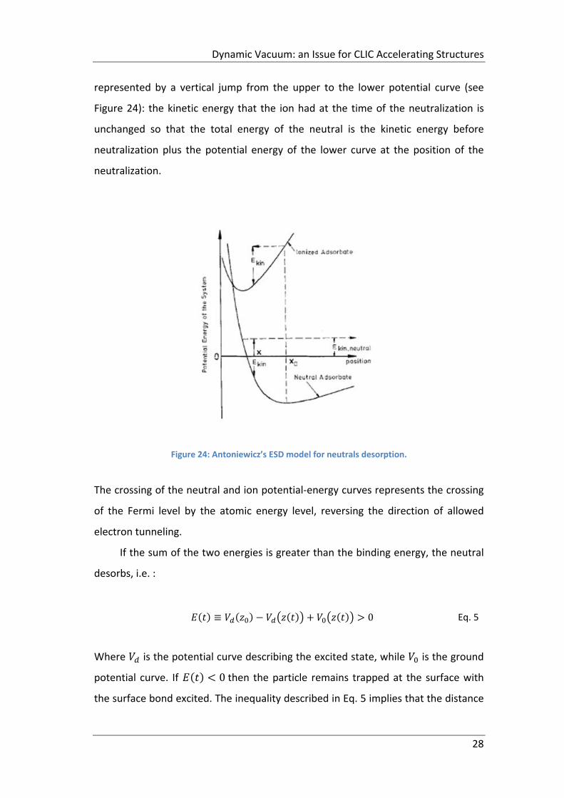
Describing desorption process for ions by means of this model is more
complicated because two tunneling processes must occur. The initial state with the
lowest threshold energy that leads to positive‐ion desorption is an excited positive
ion on the surface referred to as V2 in Figure 25. The desorption sequence, which
leads to a positive‐ion desorption, requires that the excited ions moves toward the
substrate, be neutralized sufficiently close to the substrate to be high up on curve
V0 in fig 29 and then be ionized again by electron tunneling to the substrate and find
itself on curve V1 before it leaves the close vicinity of the substrate. V1 is the
ground‐state ion potential energy curve. The rate at which electrons tunnel
between the substrate and adsorbate and vice versa depends on the relative
positions of the atomic or molecular energy level of the adsorbate and the Fermi
level of the metal substrate. At a distance from the substrate where V0 has a higher
energy than V1, the tunneling takes place from the adsorbate to the substrate and
vice versa.
In Figure 25 there is an example of a desorbing ion, following Antoniewicz’
considerations and making the assumption that the atom is initially at rest. After
the excitation to the V2 potential curve, the particle moves toward the substrate
with a classical velocity:
2/
Eq. 6
If the probability per unit time of an electron tunneling from the metal onto the ion
is R2(z), then the probability that the ion is not neutralized at the position z is:
Dynamic Vacuum: an Issue for CLIC Accelerating Structures
30
exp /′
2 / Eq. 7
Figure 25: Anoniewicz’s ESD model for ionic desorption.
The neutralized particle might desorb as a neutral, but if the particle has sufficient
total energy, then it can be reionized. The neutral has sufficient energy if
1 Eq. 8
where is the position of the ion at the time of neutralization. Consequently, for
the particle to desorb as an ion, it has to be neutralized in the region z2<zn< z1 ,
where z1 is the solution of the equation 1 and z2 is the
solution of the equation , where the two potential energy cross.
Dynamic Vacuum: an Issue for CLIC Accelerating Structures
31
Finally, an important information to be underlined is that the probability of
desorption depends sensitively on the mass of the desorbing ion (see Eq 6). The
heavier the isotope, the slower it moves so that it has a larger probability of being
captured. This isotopic effect was already described by the MGR model and first
observed by Madey. The Antoniewicz model adds that the isotope dependence of
ions is larger than that of neutrals since ion desorption is a two‐electron tunneling
process.
2.2.3 Gortel’s model
The two desorption models described above are very useful to have a simple
picture of the desorption sequences and to qualitatively interpret the experimental
data. In order to have a quantitative analysis and a better understanding of the
kinetic energy distribution of the desorbed particles a new model is needed. Gortel
described a quantum‐mechanic model named Wave Packet Squeezing model (WPS)
that could complete the previous models and calculate the kinetic energy
distribution of the desorbed particle in perfect agreement with the experimental
data.
The limits in the previous two models, according to Gortel, were related to their
qualitative nature and to the fact that no kinetic distribution was well described:
the kinetic energy distribution experimentally measured was lower than the one
forecast by the models and, in addition, in the specific case of the Antoniewicz
model, Gortel claimed that the model was suitable for describing the desorption
sequence of a physisorbed particle on metal surface instead of a chemisorbed one.
This statement was in accordance with the experimental data of desorbed atoms
and molecules from metal surface that showed that, indeed, only neutral species
were desorbed from the surface while no ionic species were encountered.
Gortel focused on the description of the desorption sequence of a physisorbed
particle on a metallic surface for which enough experimental data were available:
he observed that the incoming electron energy thresholds clearly indicate that the
valence ionization of the physisorbed atom is responsible for triggering desorption,
Dynamic Vacuum: an Issue for CLIC Accelerating Structures
32
in analogy with what described by Antoniewicz. Jennison et alii proposed that after
the first ionization a reneutralization due to tunneling effect immediately occurs so
that the neutralizing electron is occupying an excited, originally empty, orbital of
the molecule which then forms a covalent bond with the surface metal atoms.
Starting from this idea Gortel described the WPS model as follows: as a result
of the initial excitation sequence, the system is promoted to the electronic state in
which the atom is bound to the surface by a potential Vd(z) which is narrower and
deeper than the ground state potential is but has nearly the same equilibrium
position. The system evolves in this potential until an electronic de‐excitation
process returns it to the electronic ground state.
According to the classical mechanics no desorption can occur in such a scenario
because the adsorbed particle is placed with zero velocity close to the equilibrium
position of the Vd(z) so that a very little kinetic energy can be gained: therefore, is
necessary to have a closer look at the kinetic energy gain from the quantum
mechanical point of view.
Starting from a one‐dimensional model, let <A(t)> be a time‐dependent
quantum mechanical expectation value of an operator A in a quantum state
described by the wave function φ(z,t) which we take to be the wave packet evolving
along Vd(z). Taking the momentum operator p for A, the kinetic energy is described
as:
1
2⟨ ⟩ ∆ Eq. 9
Where the first term of the sum is the expected kinetic energy of the particle at a
time t in the state described by the wave packet , and ∆ is the quantum
fluctuation of momentum: so the first term is the classical contribution to the
kinetic energy , the only contribution described by the MGR and
Antoniewicz models, while the second term is purely quantum mechanical.
At low temperatures the adsorbed particle before the initial excitation is
described by the ground state potential with 0 0 and
0 0 : this is the minimum uncertainty wave packet and the
Dynamic Vacuum: an Issue for CLIC Accelerating Structures
33
momentum and position uncertainties are related by the Heisenberg equality
0 0 /2 .
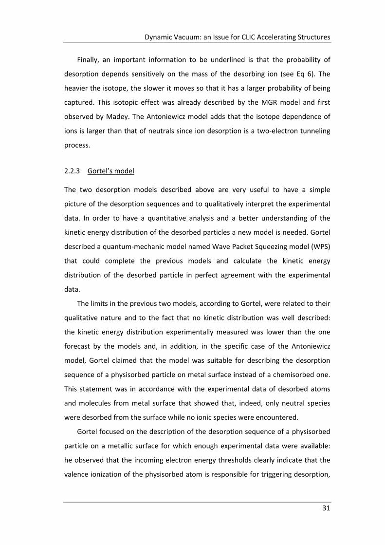
In the usual MGR scenario this wave packet is placed on a smooth part of the
potential curve so that, when the particle is accelerated toward the new minimum
position, the position uncertainty increases due to the wave packet spreading
effect (Figure 26). This simply means that, analyzing the time‐dependent solution of
the Schrodinger equation, as the particle moves along its potential is less probable
to find it in a certain place while the probability to find it in other positions
increases.
Figure 26: The wave function spreads out of time.
Due to this effect, the ∆ must decrease so that the quantum mechanical
correction to the classical MGR model is very little. The situation change drastically
in the WPS scenario: in order to understand the desorption sequence an extreme
case is described in which the equilibrium position and coincide exactly
(Figure 27).
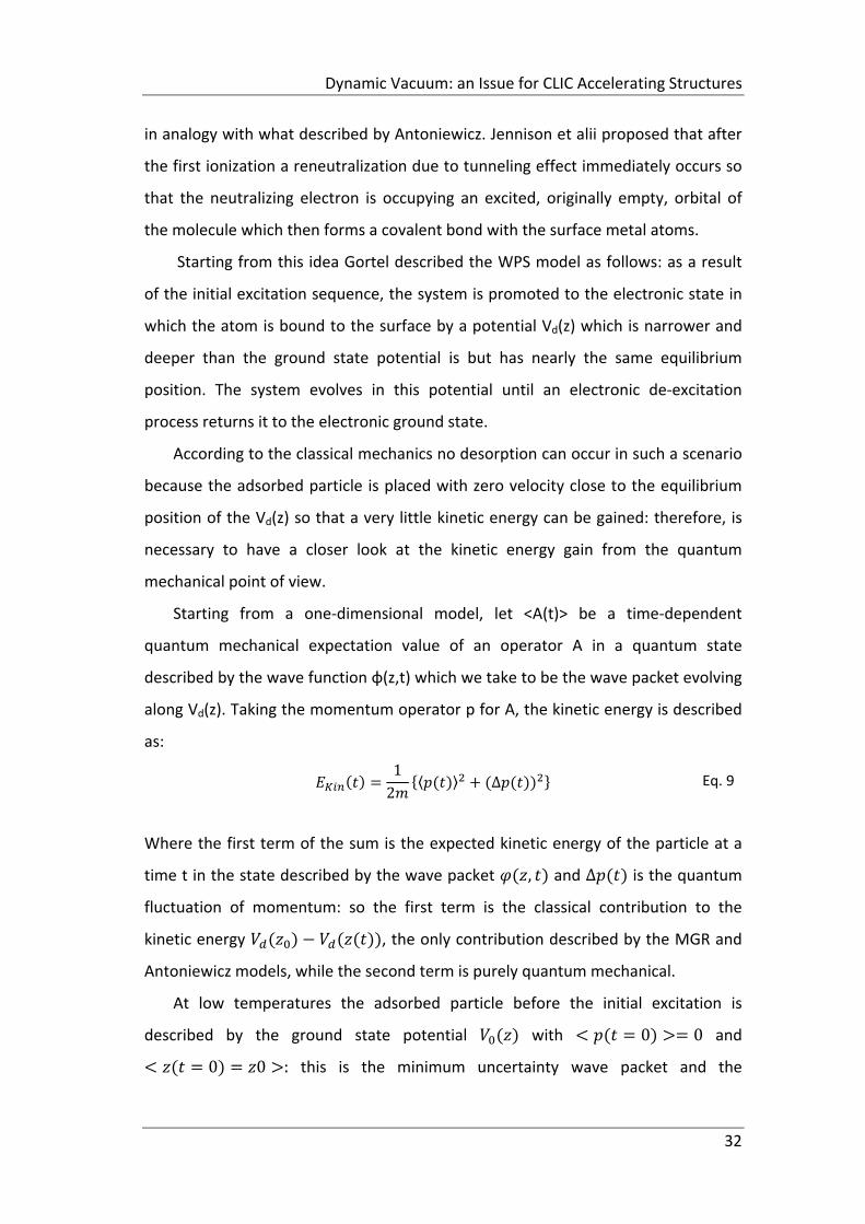
Dynamic Vacuum: an Issue for CLIC Accelerating Structures
34
Figure 27: Gortel ESD quantum – mechanical scenario.
The ground potential is chosen as the Morse potential of depth V0 while the excited
state potential is approximated by the harmonic potential characterized by the
frequency wd. The center of the packet remains at rest, so ≡ 0,
≡ 0 but ∆ decreases as shown in Figure 27 for three subsequent
instants of time. This means that ∆ must increase so that, in this extreme case,
only the quantum mechanical term of eq. 11 contributes to the kinetic energy gain.
If this gain exceed the binding energy V0 at z=z0 then the particle desorbs.
So the energetic condition for a particle to desorb in this model is defined as
follows:
≡1
2∆ ∆ 0 0 Eq. 10
A precise estimation of the ∆ contribution requires solving the time‐dependent
Schrodinger equation.
Detailed calculation of yields and kinetic energy distributions requires finding an
overlap between the time dependent wave packet and the continuum wave
function corresponding to the 2⁄ energy. An example of this
calculation is shown in Figure 28.
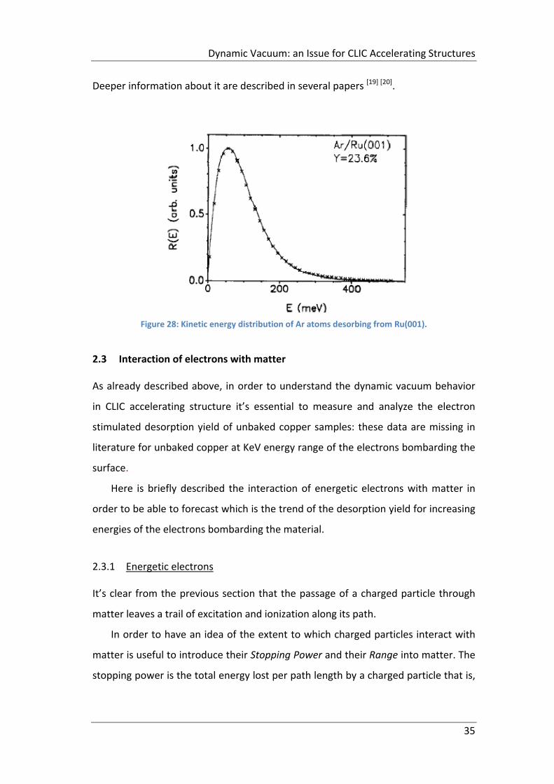
Dynamic Vacuum: an Issue for CLIC Accelerating Structures
35
Deeper information about it are described in several papers [19] [20].
Figure 28: Kinetic energy distribution of Ar atoms desorbing from Ru(001).
2.3 Interaction of electrons with matter
As already described above, in order to understand the dynamic vacuum behavior
in CLIC accelerating structure it’s essential to measure and analyze the electron
stimulated desorption yield of unbaked copper samples: these data are missing in
literature for unbaked copper at KeV energy range of the electrons bombarding the
surface.
Here is briefly described the interaction of energetic electrons with matter in
order to be able to forecast which is the trend of the desorption yield for increasing
energies of the electrons bombarding the material.
2.3.1 Energetic electrons
It’s clear from the previous section that the passage of a charged particle through
matter leaves a trail of excitation and ionization along its path.
In order to have an idea of the extent to which charged particles interact with
matter is useful to introduce their Stopping Power and their Range into matter. The
stopping power is the total energy lost per path length by a charged particle that is,
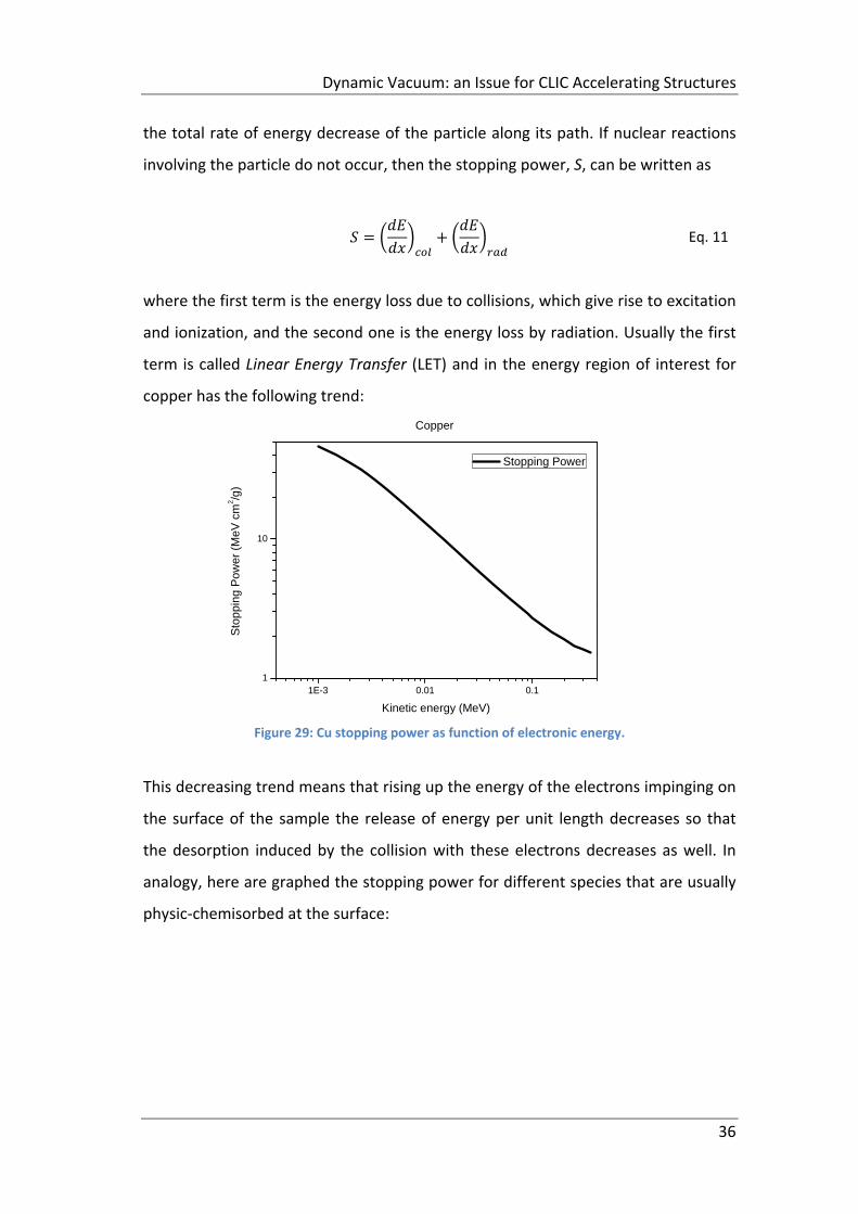
Dynamic Vacuum: an Issue for CLIC Accelerating Structures
36
the total rate of energy decrease of the particle along its path. If nuclear reactions
involving the particle do not occur, then the stopping power, S, can be written as
Eq. 11
where the first term is the energy loss due to collisions, which give rise to excitation
and ionization, and the second one is the energy loss by radiation. Usually the first
term is called Linear Energy Transfer (LET) and in the energy region of interest for
copper has the following trend:
Figure 29: Cu stopping power as function of electronic energy.
This decreasing trend means that rising up the energy of the electrons impinging on
the surface of the sample the release of energy per unit length decreases so that
the desorption induced by the collision with these electrons decreases as well. In
analogy, here are graphed the stopping power for different species that are usually
physic‐chemisorbed at the surface:
1E-3 0.01 0.11
10
Sto
ppin
g P
ow
er
(MeV
cm
2/g
)
Kinetic energy (MeV)
Stopping Power
Copper
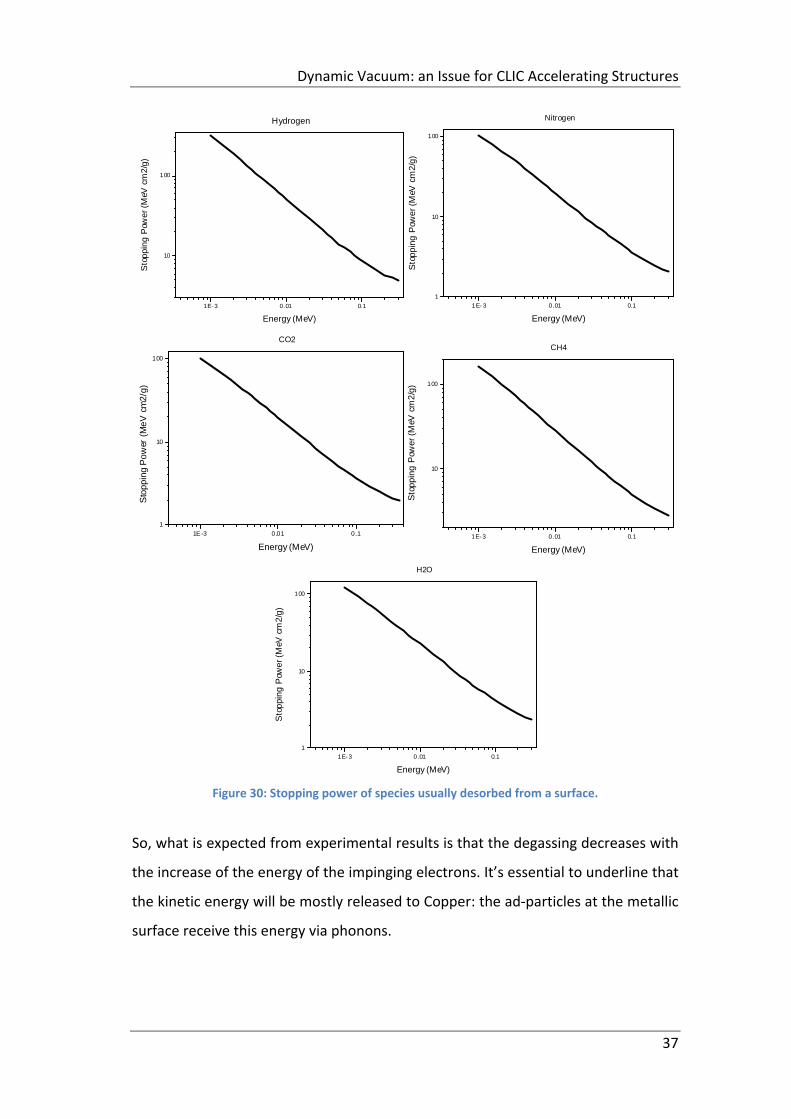
Dynamic Vacuum: an Issue for CLIC Accelerating Structures
37
Figure 30: Stopping power of species usually desorbed from a surface.
So, what is expected from experimental results is that the degassing decreases with
the increase of the energy of the impinging electrons. It’s essential to underline that
the kinetic energy will be mostly released to Copper: the ad‐particles at the metallic
surface receive this energy via phonons.
1E- 3 0.01 0.1
10
100
Sto
ppi
ng
Pow
er (
MeV
cm
2/g
)
Energy (MeV)
Hydrogen
1E- 3 0.01 0.1
1
10
100
Sto
pp
ing
Pow
er
(MeV
cm
2/g
)
Energy (MeV)
Nitrogen
1E-3 0.01 0.1
1
10
100
Sto
pp
ing
Po
wer
(M
eV
cm
2/g
)
Energy (MeV)
CO2
1E- 3 0.01 0.1
10
100
Sto
pp
ing
Pow
er (M
eV c
m2
/g)
Energy (MeV)
CH4
1E- 3 0.01 0.1
1
10
100
Sto
ppi
ng
Pow
er (
MeV
cm
2/g
)
Energy (MeV)
H2O
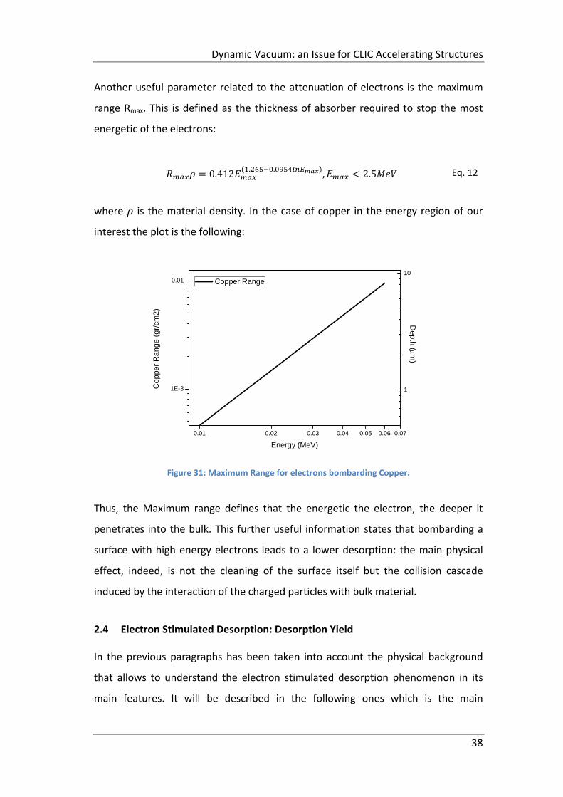
Dynamic Vacuum: an Issue for CLIC Accelerating Structures
38
Another useful parameter related to the attenuation of electrons is the maximum
range Rmax. This is defined as the thickness of absorber required to stop the most
energetic of the electrons:
0.412. .
, 2.5 Eq. 12
where is the material density. In the case of copper in the energy region of our
interest the plot is the following:
0.01 0.02 0.03 0.04 0.05 0.06 0.07
1E-3
0.01
Cop
per
Ran
ge (
gr/c
m2)
Energy (MeV)
Copper Range
1
10
Depth (m
)
Figure 31: Maximum Range for electrons bombarding Copper.
Thus, the Maximum range defines that the energetic the electron, the deeper it
penetrates into the bulk. This further useful information states that bombarding a
surface with high energy electrons leads to a lower desorption: the main physical
effect, indeed, is not the cleaning of the surface itself but the collision cascade
induced by the interaction of the charged particles with bulk material.
2.4 Electron Stimulated Desorption: Desorption Yield
In the previous paragraphs has been taken into account the physical background
that allows to understand the electron stimulated desorption phenomenon in its
main features. It will be described in the following ones which is the main
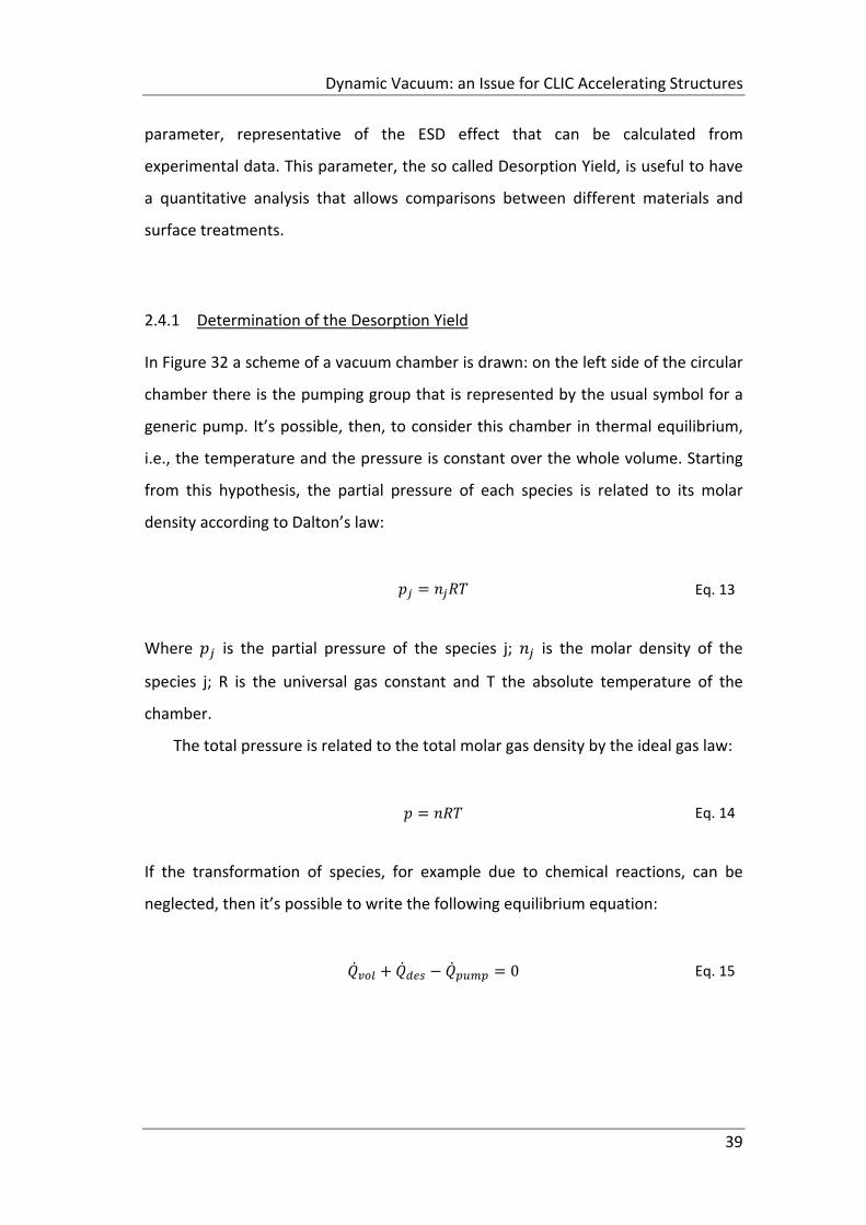
Dynamic Vacuum: an Issue for CLIC Accelerating Structures
39
parameter, representative of the ESD effect that can be calculated from
experimental data. This parameter, the so called Desorption Yield, is useful to have
a quantitative analysis that allows comparisons between different materials and
surface treatments.
2.4.1 Determination of the Desorption Yield
In Figure 32 a scheme of a vacuum chamber is drawn: on the left side of the circular
chamber there is the pumping group that is represented by the usual symbol for a
generic pump. It’s possible, then, to consider this chamber in thermal equilibrium,
i.e., the temperature and the pressure is constant over the whole volume. Starting
from this hypothesis, the partial pressure of each species is related to its molar
density according to Dalton’s law:
Eq. 13
Where is the partial pressure of the species j; is the molar density of the
species j; R is the universal gas constant and T the absolute temperature of the
chamber.
The total pressure is related to the total molar gas density by the ideal gas law:
Eq. 14
If the transformation of species, for example due to chemical reactions, can be
neglected, then it’s possible to write the following equilibrium equation:
0 Eq. 15
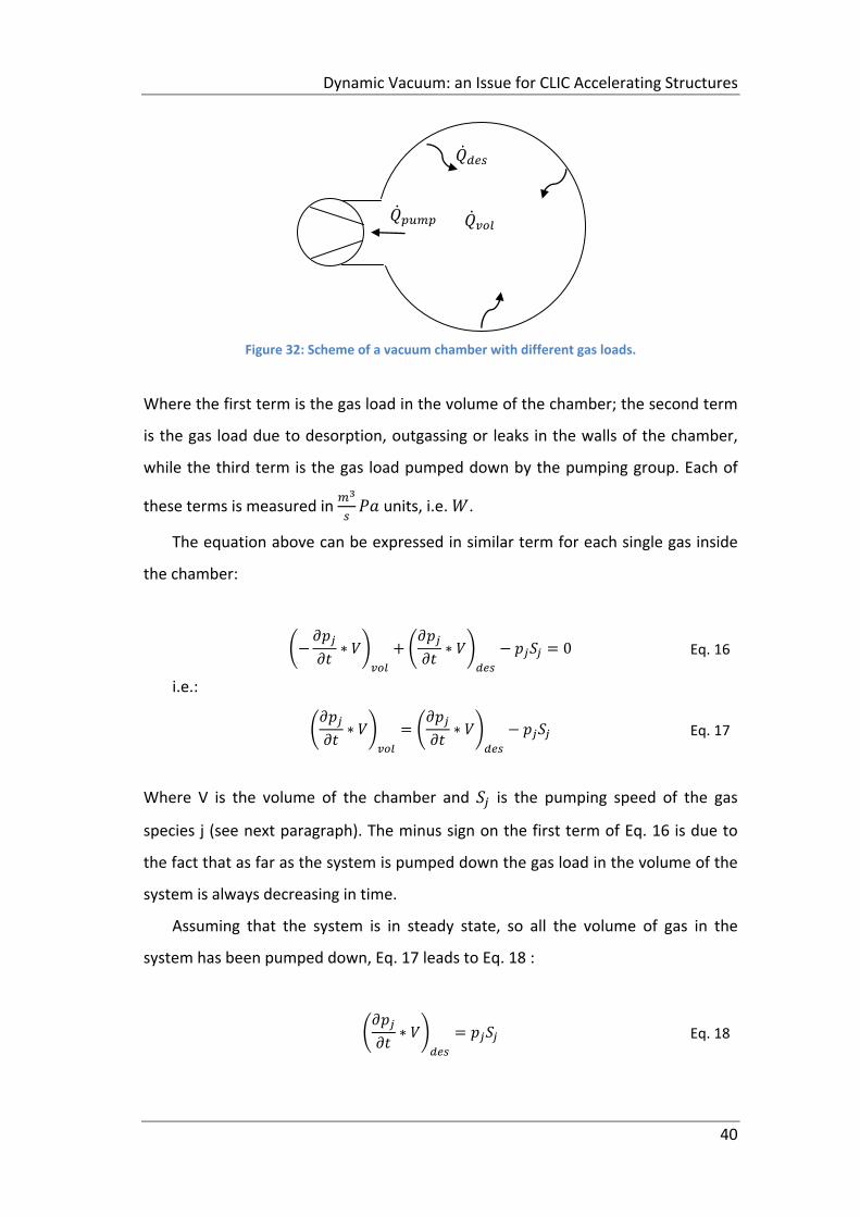
Dynamic Vacuum: an Issue for CLIC Accelerating Structures
40
Figure 32: Scheme of a vacuum chamber with different gas loads.
Where the first term is the gas load in the volume of the chamber; the second term
is the gas load due to desorption, outgassing or leaks in the walls of the chamber,
while the third term is the gas load pumped down by the pumping group. Each of
these terms is measured in units, i.e. .
The equation above can be expressed in similar term for each single gas inside
the chamber:
∗ ∗ 0 Eq. 16
i.e.:
∗ ∗ Eq. 17
Where V is the volume of the chamber and is the pumping speed of the gas
species j (see next paragraph). The minus sign on the first term of Eq. 16 is due to
the fact that as far as the system is pumped down the gas load in the volume of the
system is always decreasing in time.
Assuming that the system is in steady state, so all the volume of gas in the
system has been pumped down, Eq. 17 leads to Eq. 18 :
∗ Eq. 18
Dynamic Vacuum: an Issue for CLIC Accelerating Structures
41
The equation above states that if a gas burst due to electron impinging on the
surface of the chamber occurs then each gas species is pumped down by the
pumping group with its specific pumping speed.
Without the ESD effect, the vacuum chamber reaches the steady state
condition with a background pressure . The desorption of gas molecules
adsorbed on the surface of the vacuum chamber represents just an additional gas
load to the system so that with a gas burst due to the electron stimulated
desorption another equilibrium pressure is reached, .
The increase of pressure due to the electron stimulated desorption can be
defined by the following relation:
Eq. 19
where is the molecular desorption yield in #
unit, i.e. number of molecules
released per impinging electron; is the electron current bombarding the surface in
A unit; e is the elementary charge and k the Boltzmann constant. The fraction
gives the number of electrons impinging on the surface so that the term is the
number of molecules released per unit time.
From Eq. 19, the desorption yield is defined as:
Eq. 20
and usually it’s plotted against the dose of electron received by the surface per
square centimeter.
In Figure 33, a typical desorption curve is graphed: in this graph the desorption
yield of a non baked copper sample is calculated from experimental data with a
biasing of the sample at 0.35 KV. The trend of the curve is decreasing due to the fact
that as the sample is tested all the ad‐particles at the surface are released little by
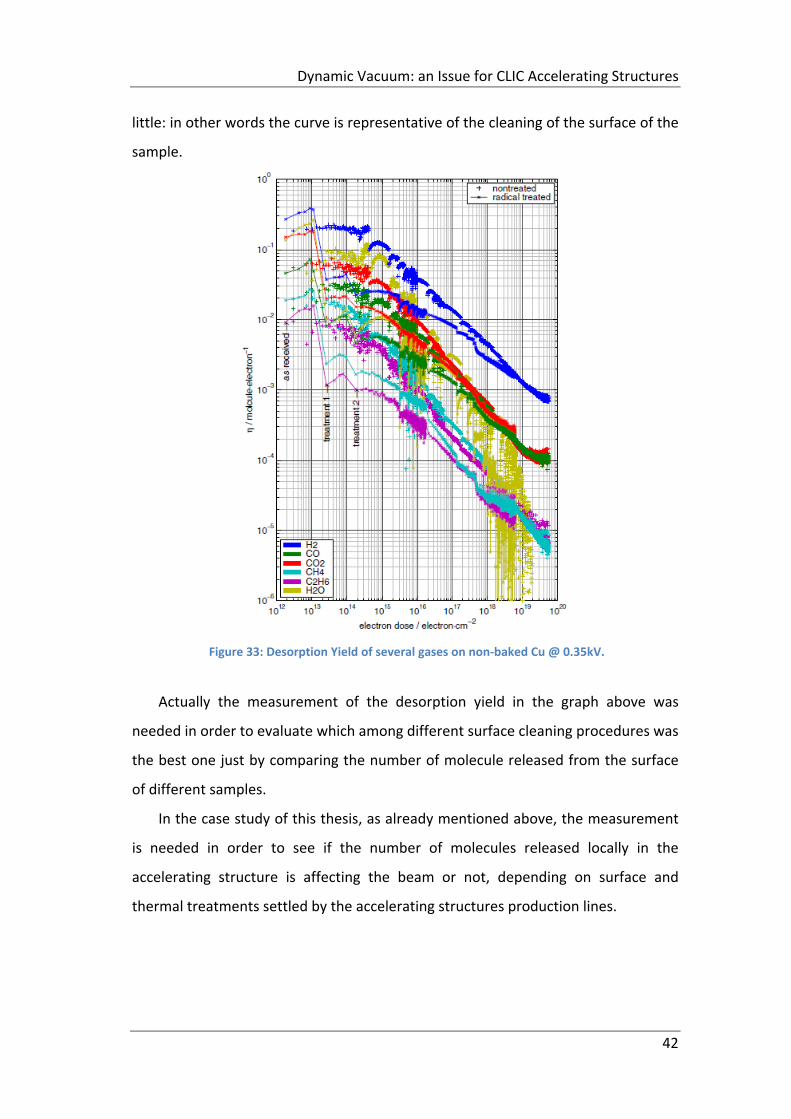
Dynamic Vacuum: an Issue for CLIC Accelerating Structures
42
little: in other words the curve is representative of the cleaning of the surface of the
sample.
Figure 33: Desorption Yield of several gases on non‐baked Cu @ 0.35kV.
Actually the measurement of the desorption yield in the graph above was
needed in order to evaluate which among different surface cleaning procedures was
the best one just by comparing the number of molecule released from the surface
of different samples.
In the case study of this thesis, as already mentioned above, the measurement
is needed in order to see if the number of molecules released locally in the
accelerating structure is affecting the beam or not, depending on surface and
thermal treatments settled by the accelerating structures production lines.
Dynamic Vacuum: an Issue for CLIC Accelerating Structures
43
2.4.2 Conductance and volume throughput
Since the pumping speed and the conductance of a vacuum system have already
been mentioned several times, it’s worthy to give a description of it.
Usually, in vacuum science and technology the gas flow rate is expressed as a
throughput in pressure‐volume units:
Eq. 21
At a particular pressure,
Eq. 22
where is the pumping speed, or volume throughput.
When a pumping group is connected to a vacuum system, the actual pumping
speed of the pump is reduced by the restrictions due to connecting pipework. Thus,
the geometry of the system itself is playing an important role from vacuum point of
view. Furthermore, in order to calculate a correct desorption yield, the pumping
speed of each gaseous component released must be known.
Aiming at calculating the loss in the pumping speed, Knudsen first introduced
the concept of a pipe as an impedance or resistance in electrical sense defining a
conductance as:
Eq. 23
where is the upstream pressure and the downstream one. Therefore, the
resistance is defined as:
1 Eq. 24
Dynamic Vacuum: an Issue for CLIC Accelerating Structures
44
Applying this concept to a set of pipes or components in series, the net conductance
is found from:
1 1 1 1
⋯ Eq. 25
Finally the net speed of a pump in series with a component or pipe is found in a
similar way:
1 1 1
Eq. 26
Expressions for conductance are usefully formulated in terms of transmission
probability, so that the conductance of a duct (or other component) is given by the
entrance aperture conductance times the transmission probability:
Eq. 27
The aperture conductance is dependent on the area of the orifice and on the
molar mass of the gaseous specie. Therefore, is more difficult to pump down bigger
molecules:
2
Eq. 28
The transmission probability can be described by different expressions, depending
on the geometry of the duct: for example, for long ducts, the Eq. 29 is commonly
used.
4
3
Eq. 29
Where d, is the diameter of the duct and l its length.
Dynamic Vacuum: an Issue for CLIC Accelerating Structures
45
For shorter ducts, the long duct relation leads to an overestimation of the
conductance. Therefore the transmission probability is described as follows:
1
Eq. 30
Pumping speed and conductance calculations for the experimental set up built for
desorption yield measurement is quoted in chapter 4.
Copper samples specifications
46
CHAPTER 3
COPPER SAMPLES SPECIFICATIONS
All copper samples have been treated following different production lines designed
for CLIC accelerating structures. These different treatments are still under study in
order to see which is the best from the chemical‐physical and mechanical properties
point of view and, last but not least, from the economical point of view.
The test accelerating structures produced up to now are diamond turned
structures made of Oxygen Free Electronic grade copper. In Figure 34, an example
of one RF design for the above mentioned structures is shown. In the center of the
structure there is the bore hole where the electron beam is supposed to accelerate,
and the cross dividing the structure in four quarters is made of damping material,
i.e. SiC, which absorb higher order frequencies that are not useful to accelerate the
beam.
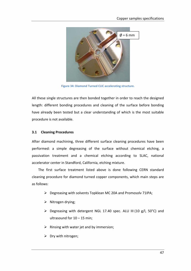
Copper samples specifications
47
Figure 34: Diamond Turned CLIC accelerating structure.
All these single structures are then bonded together in order to reach the designed
length: different bonding procedures and cleaning of the surface before bonding
have already been tested but a clear understanding of which is the most suitable
procedure is not available.
3.1 Cleaning Procedures
After diamond machining, three different surface cleaning procedures have been
performed: a simple degreasing of the surface without chemical etching, a
passivation treatment and a chemical etching according to SLAC, national
accelerator center in Standford, California, etching mixture.
The first surface treatment listed above is done following CERN standard
cleaning procedure for diamond turned copper components, which main steps are
as follows:
Degreasing with solvents Topklean MC 20A and Promosolv 71IPA;
Nitrogen drying;
Degreasing with detergent NGL 17.40 spec. ALU III (10 g/l, 50°C) and
ultrasound for 10 – 15 min;
Rinsing with water jet and by immersion;
Dry with nitrogen;
Ø = 6 mm
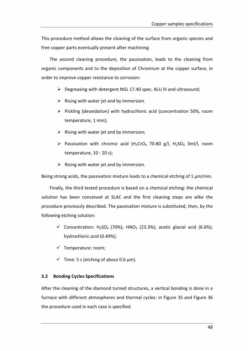
Copper samples specifications
48
This procedure method allows the cleaning of the surface from organic species and
free copper parts eventually present after machining.
The second cleaning procedure, the passivation, leads to the cleaning from
organic components and to the deposition of Chromium at the copper surface, in
order to improve copper resistance to corrosion:
Degreasing with detergent NGL 17.40 spec. ALU III and ultrasound;
Rising with water jet and by immersion.
Pickling (deoxidation) with hydrochloric acid (concentration 50%, room
temperature, 1 min);
Rising with water jet and by immersion;
Passivation with chromic acid (H2CrO4 70‐80 g/l, H2SO4 3ml/l, room
temperature, 10 ‐ 20 s);
Rising with water jet and by immersion.
Being strong acids, the passivation mixture leads to a chemical etching of 1 µm/min.
Finally, the third tested procedure is based on a chemical etching: the chemical
solution has been conceived at SLAC and the first cleaning steps are alike the
procedure previously described. The passivation mixture is substituted, then, by the
following etching solution:
Concentration: H2SO4 (70%); HNO3 (23.3%); acetic glacial acid (6.6%);
hydrochloric acid (0.49%);
Temperature: room;
Time: 5 s (etching of about 0.6 µm).
3.2 Bonding Cycles Specifications
After the cleaning of the diamond turned structures, a vertical bonding is done in a
furnace with different atmospheres and thermal cycles: in Figure 35 and Figure 36
the procedure used in each case is specified.
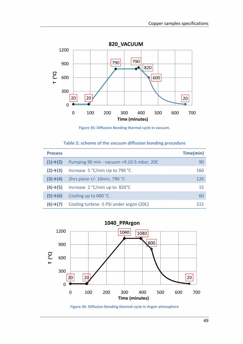
Copper samples specifications
49
Figure 35: Diffusion Bonding thermal cycle in vacuum.
Table 2: scheme of the vacuum diffusion bonding procedure
Process Time(min)
(1)→(2) Pumping 90 min ‐ vacuum <9.10‐5 mbar, 20C 90
(2)→(3) Increase 5 °C/min Up to 790 °C 160
(3)→(4) 2hrs piece +/‐ 10min, 790 °C 120
(4)→(5) Increase 2 °C/min up to 820°C 15
(5)→(6) Cooling up to 600 °C 60
(6)→(7) Cooling turbine ‐5 PSI under argon (20C) 215
Figure 36: Diffusion Bonding thermal cycle in Argon atmosphere
20 20
790 790820
600
20
0
300
600
900
1200
0 100 200 300 400 500 600 700
T (°C)
Time (minutes)
820_VACUUM
20 20
1040 1040
800
20
0
300
600
900
1200
0 100 200 300 400 500 600 700
T (°C)
Time (minutes)
1040_PPArgon
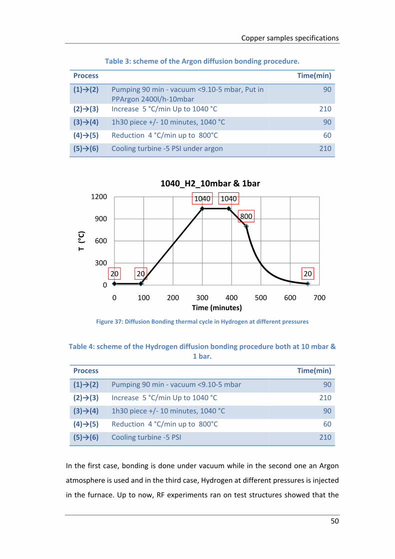
Copper samples specifications
50
Table 3: scheme of the Argon diffusion bonding procedure.
Process Time(min)
(1)→(2) Pumping 90 min ‐ vacuum <9.10‐5 mbar, Put in PPArgon 2400l/h‐10mbar
90
(2)→(3) Increase 5 °C/min Up to 1040 °C 210
(3)→(4) 1h30 piece +/‐ 10 minutes, 1040 °C 90
(4)→(5) Reduction 4 °C/min up to 800°C 60
(5)→(6) Cooling turbine ‐5 PSI under argon 210
Figure 37: Diffusion Bonding thermal cycle in Hydrogen at different pressures
Table 4: scheme of the Hydrogen diffusion bonding procedure both at 10 mbar & 1 bar.
Process Time(min)
(1)→(2) Pumping 90 min ‐ vacuum <9.10‐5 mbar 90
(2)→(3) Increase 5 °C/min Up to 1040 °C 210
(3)→(4) 1h30 piece +/‐ 10 minutes, 1040 °C 90
(4)→(5) Reduction 4 °C/min up to 800°C 60
(5)→(6) Cooling turbine ‐5 PSI 210
In the first case, bonding is done under vacuum while in the second one an Argon
atmosphere is used and in the third case, Hydrogen at different pressures is injected
in the furnace. Up to now, RF experiments ran on test structures showed that the
20 20
1040 1040
800
20
0
300
600
900
1200
0 100 200 300 400 500 600 700
T (°C)
Time (minutes)
1040_H2_10mbar & 1bar
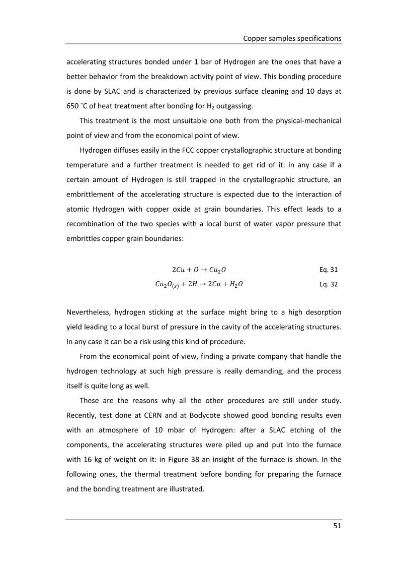
Copper samples specifications
51
accelerating structures bonded under 1 bar of Hydrogen are the ones that have a
better behavior from the breakdown activity point of view. This bonding procedure
is done by SLAC and is characterized by previous surface cleaning and 10 days at
650 ˚C of heat treatment after bonding for H2 outgassing.
This treatment is the most unsuitable one both from the physical‐mechanical
point of view and from the economical point of view.
Hydrogen diffuses easily in the FCC copper crystallographic structure at bonding
temperature and a further treatment is needed to get rid of it: in any case if a
certain amount of Hydrogen is still trapped in the crystallographic structure, an
embrittlement of the accelerating structure is expected due to the interaction of
atomic Hydrogen with copper oxide at grain boundaries. This effect leads to a
recombination of the two species with a local burst of water vapor pressure that
embrittles copper grain boundaries:
2 → Eq. 31
2 → 2 Eq. 32
Nevertheless, hydrogen sticking at the surface might bring to a high desorption
yield leading to a local burst of pressure in the cavity of the accelerating structures.
In any case it can be a risk using this kind of procedure.
From the economical point of view, finding a private company that handle the
hydrogen technology at such high pressure is really demanding, and the process
itself is quite long as well.
These are the reasons why all the other procedures are still under study.
Recently, test done at CERN and at Bodycote showed good bonding results even
with an atmosphere of 10 mbar of Hydrogen: after a SLAC etching of the
components, the accelerating structures were piled up and put into the furnace
with 16 kg of weight on it: in Figure 38 an insight of the furnace is shown. In the
following ones, the thermal treatment before bonding for preparing the furnace
and the bonding treatment are illustrated.
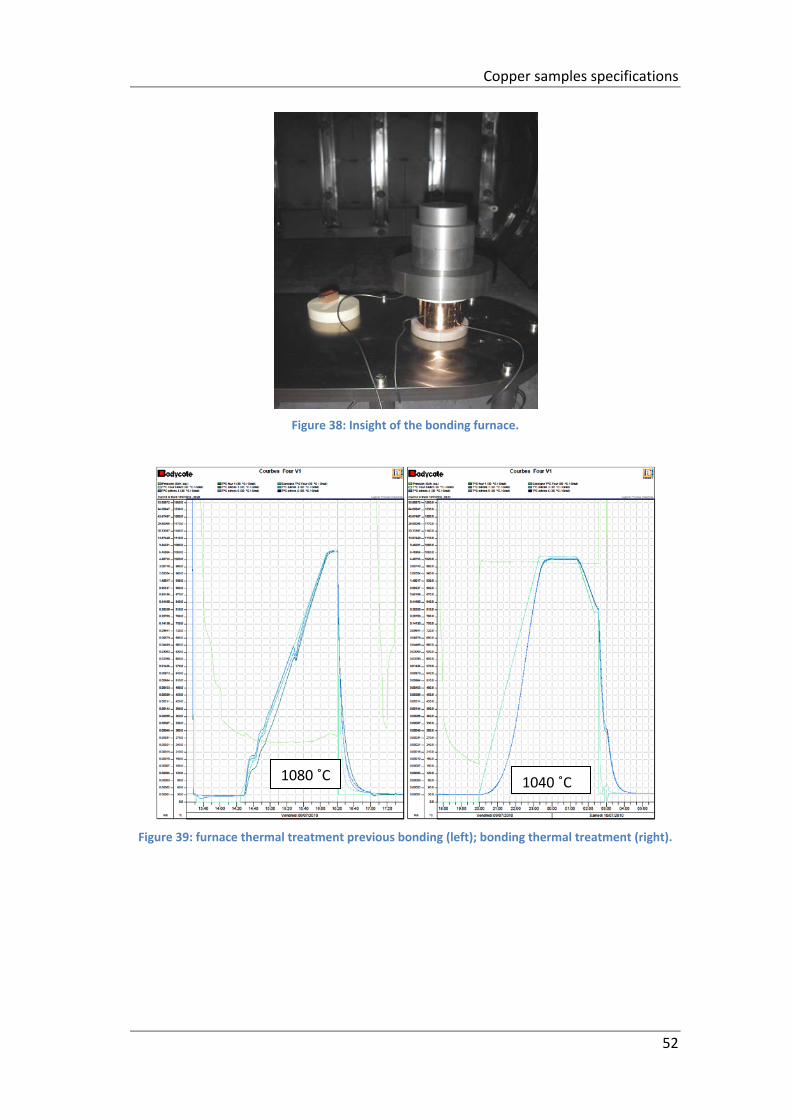
Copper samples specifications
52
Figure 38: Insight of the bonding furnace.
Figure 39: furnace thermal treatment previous bonding (left); bonding thermal treatment (right).
1080 ˚C 1040 ˚C
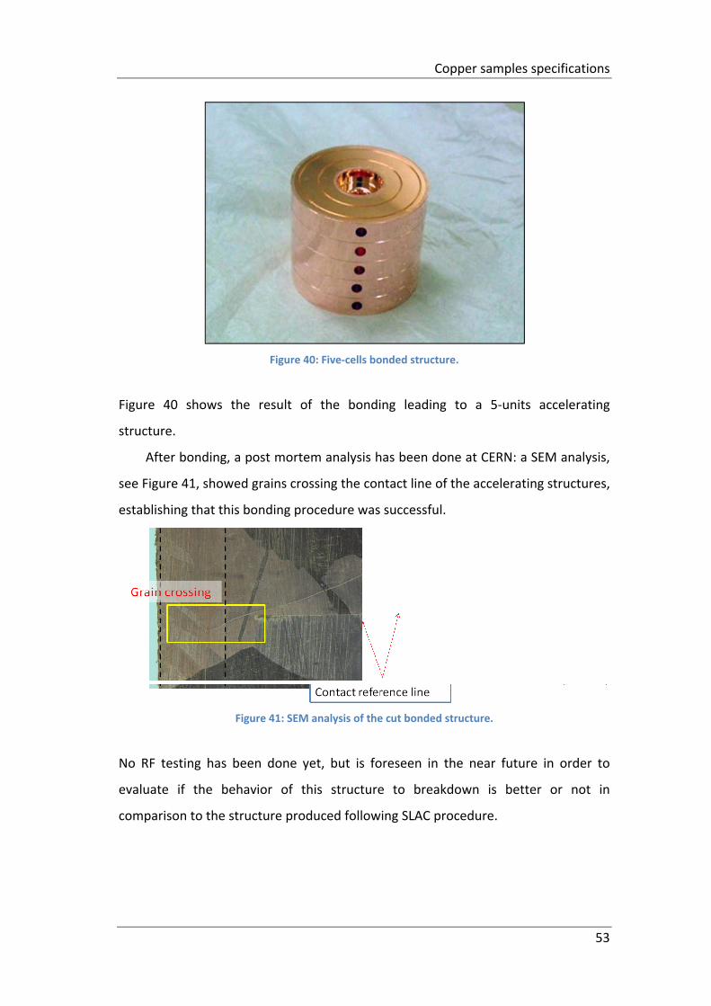
Copper samples specifications
53
Figure 40: Five‐cells bonded structure.
Figure 40 shows the result of the bonding leading to a 5‐units accelerating
structure.
After bonding, a post mortem analysis has been done at CERN: a SEM analysis,
see Figure 41, showed grains crossing the contact line of the accelerating structures,
establishing that this bonding procedure was successful.
Figure 41: SEM analysis of the cut bonded structure.
No RF testing has been done yet, but is foreseen in the near future in order to
evaluate if the behavior of this structure to breakdown is better or not in
comparison to the structure produced following SLAC procedure.
Copper samples specifications
54
3.3 Diffusion Profile Calculations
Aiming at calculating the actual amount of hydrogen introduced by these bonding
procedures inside copper, a diffusion profile calculation has been developed. The
analysis is focused on Hydrogen content being the most dangerous element
introduced during bonding procedure.
3.3.1 Copper – Hydrogen interactions
When molecular hydrogen interacts with copper, temperature induced diffusion
occurs, leading to an increase of the content of atomic hydrogen inside the
crystallographic copper structure. A peculiar aspect of hydrogen‐copper interaction
is that copper is known to be an endothermic material with respect to hydrogen. In
order to understand this concept is useful to introduce the definition of the
solubility of atomic hydrogen in copper.
In order to have diffusion of hydrogen into a solid structure, first dissolution
from molecular to atomic hydrogen at the solid surface is needed:
M2
→ ∆ Eq. 33
where is the number of moles of hydrogen and ∆ is the solution enthalpy per
mole. This latter term takes into account the heat release per adsorbed hydrogen
atom.
At the equilibrium, the chemical potentials of molecular hydrogen in the
gaseous atmosphere and the atomic hydrogen dissolved in copper must be equal:
μ1
2μ Eq. 34
Introducing the definition of the chemical potential for an ideal gaseous phase and
Sievert’s law, Eq. 34 turns out to be:
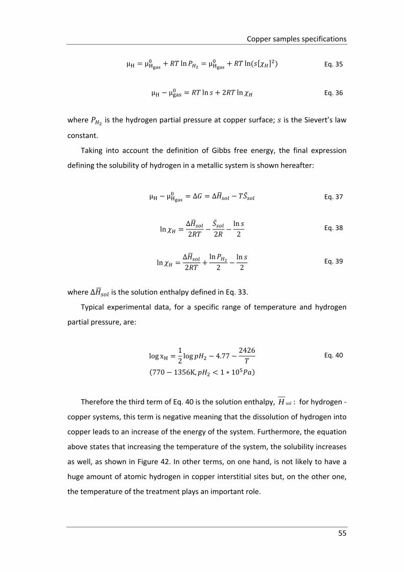
Copper samples specifications
55
μ μ ln μ ln Eq. 35
μ μ ln 2 ln Eq. 36
where is the hydrogen partial pressure at copper surface; is the Sievert’s law
constant.
Taking into account the definition of Gibbs free energy, the final expression
defining the solubility of hydrogen in a metallic system is shown hereafter:
μ μ ∆ ∆ Eq. 37
ln∆
2
2
ln
2 Eq. 38
ln∆
2
ln
2
ln
2 Eq. 39
where ∆ is the solution enthalpy defined in Eq. 33.
Typical experimental data, for a specific range of temperature and hydrogen
partial pressure, are:
log x1
2log 4.77
2426 Eq. 40
770 1356K, 1 ∗ 10
Therefore the third term of Eq. 40 is the solution enthalpy, solH : for hydrogen ‐
copper systems, this term is negative meaning that the dissolution of hydrogen into
copper leads to an increase of the energy of the system. Furthermore, the equation
above states that increasing the temperature of the system, the solubility increases
as well, as shown in Figure 42. In other terms, on one hand, is not likely to have a
huge amount of atomic hydrogen in copper interstitial sites but, on the other one,
the temperature of the treatment plays an important role.
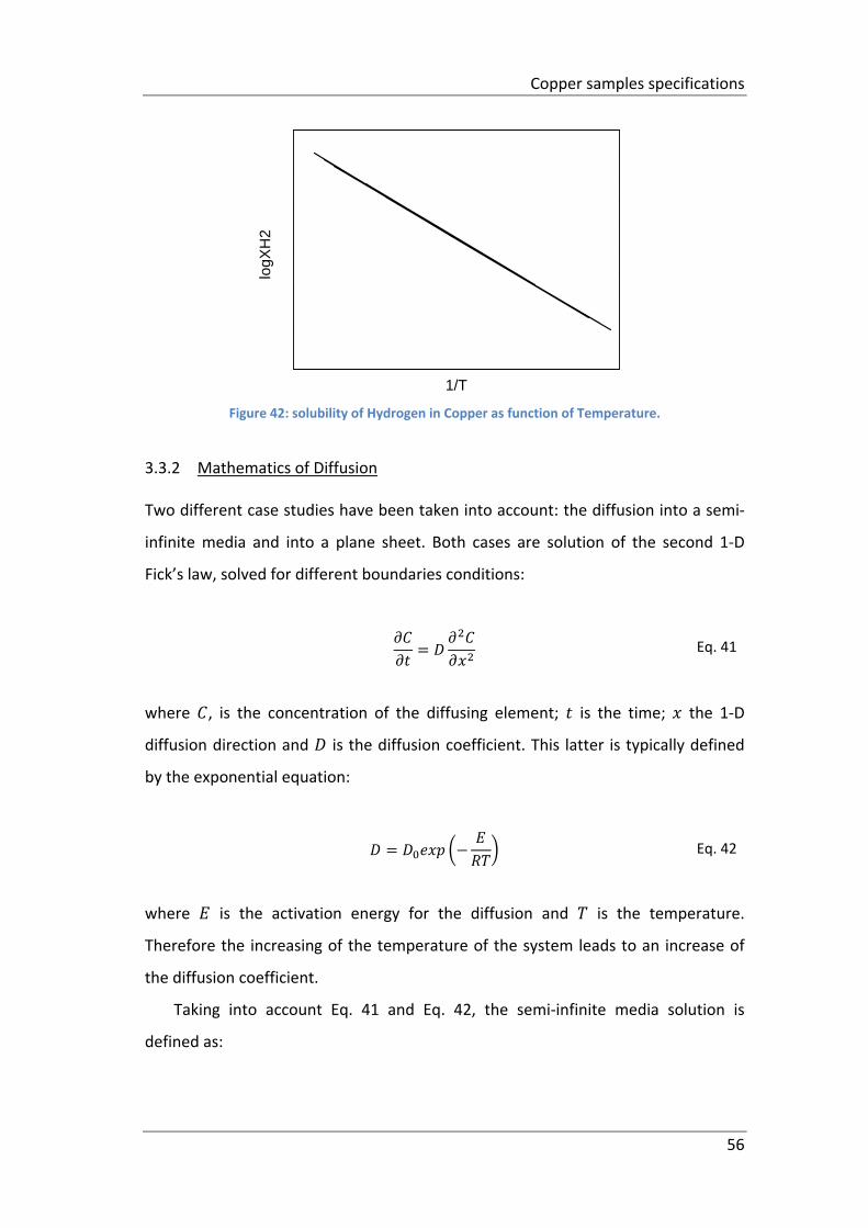
Copper samples specifications
56
Figure 42: solubility of Hydrogen in Copper as function of Temperature.
3.3.2 Mathematics of Diffusion
Two different case studies have been taken into account: the diffusion into a semi‐
infinite media and into a plane sheet. Both cases are solution of the second 1‐D
Fick’s law, solved for different boundaries conditions:
Eq. 41
where , is the concentration of the diffusing element; is the time; the 1‐D
diffusion direction and is the diffusion coefficient. This latter is typically defined
by the exponential equation:
Eq. 42
where is the activation energy for the diffusion and is the temperature.
Therefore the increasing of the temperature of the system leads to an increase of
the diffusion coefficient.
Taking into account Eq. 41 and Eq. 42, the semi‐infinite media solution is
defined as:
log
XH
2
1/T
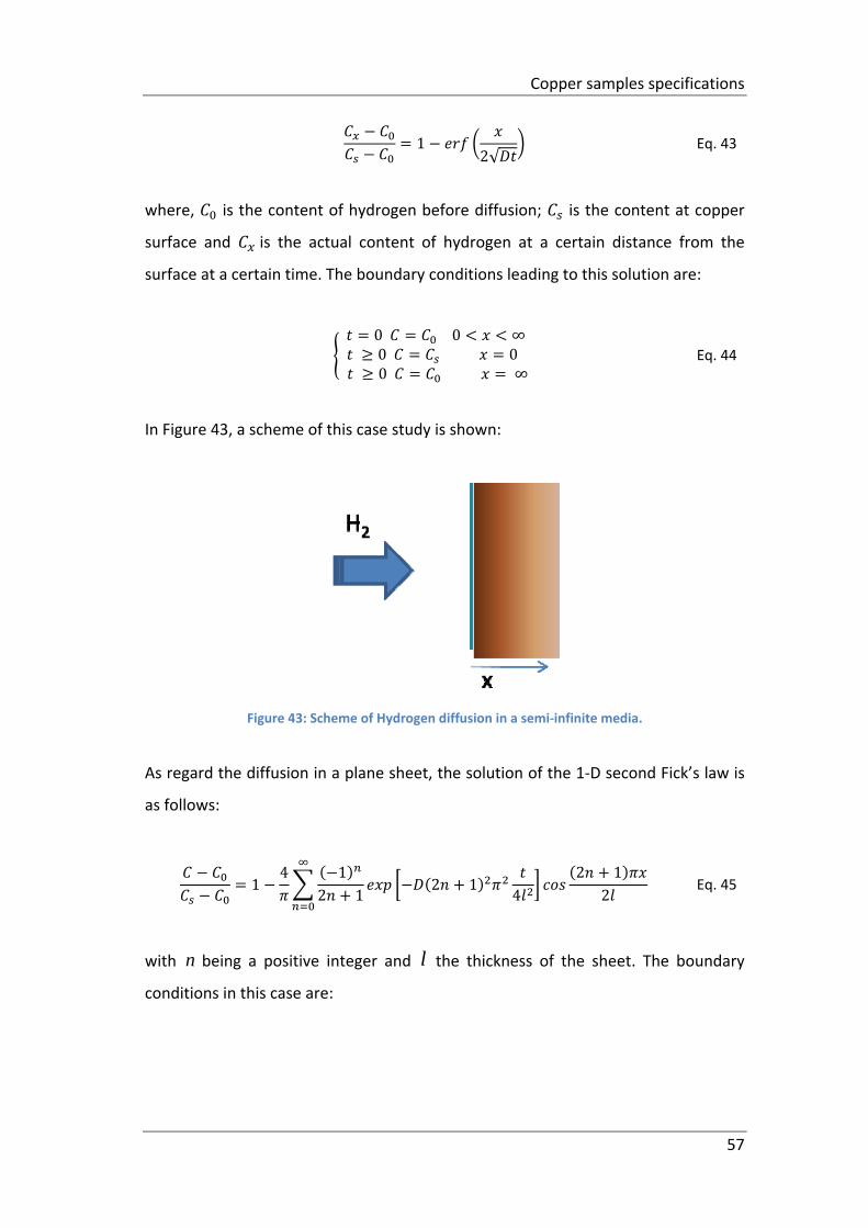
Copper samples specifications
57
12√
Eq. 43
where, is the content of hydrogen before diffusion; is the content at copper
surface and is the actual content of hydrogen at a certain distance from the
surface at a certain time. The boundary conditions leading to this solution are:
0 0 ∞ 0 0 0 ∞
Eq. 44
In Figure 43, a scheme of this case study is shown:
Figure 43: Scheme of Hydrogen diffusion in a semi‐infinite media.
As regard the diffusion in a plane sheet, the solution of the 1‐D second Fick’s law is
as follows:
14 1
2 12 1
4
2 1
2 Eq. 45
with n being a positive integer and l the thickness of the sheet. The boundary
conditions in this case are:
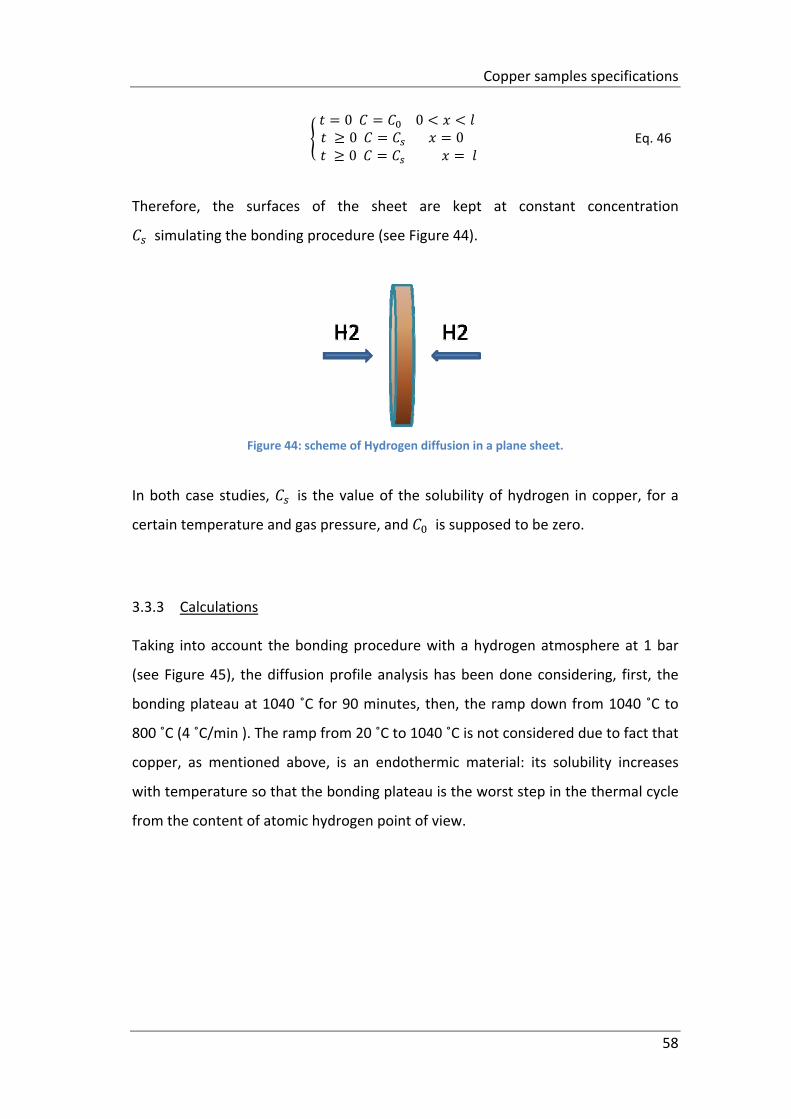
Copper samples specifications
58
0 0 0 0 0
Eq. 46
Therefore, the surfaces of the sheet are kept at constant concentration
simulating the bonding procedure (see Figure 44).
Figure 44: scheme of Hydrogen diffusion in a plane sheet.
In both case studies, is the value of the solubility of hydrogen in copper, for a
certain temperature and gas pressure, and is supposed to be zero.
3.3.3 Calculations
Taking into account the bonding procedure with a hydrogen atmosphere at 1 bar
(see Figure 45), the diffusion profile analysis has been done considering, first, the
bonding plateau at 1040 ˚C for 90 minutes, then, the ramp down from 1040 ˚C to
800 ˚C (4 ˚C/min ). The ramp from 20 ˚C to 1040 ˚C is not considered due to fact that
copper, as mentioned above, is an endothermic material: its solubility increases
with temperature so that the bonding plateau is the worst step in the thermal cycle
from the content of atomic hydrogen point of view.
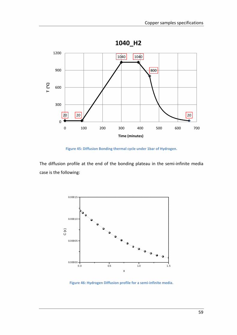
Copper samples specifications
59
Figure 45: Diffusion Bonding thermal cycle under 1bar of Hydrogen.
The diffusion profile at the end of the bonding plateau in the semi‐infinite media
case is the following:
Figure 46: Hydrogen Diffusion profile for a semi‐infinite media.
20 20
1040 1040
800
20
0
300
600
900
1200
0 100 200 300 400 500 600 700
T (°C)
Time (minutes)
1040_H2
0.0 0.5 1.0 1.5
0.00000
0.00005
0.00010
0.00015
C (x
)
x
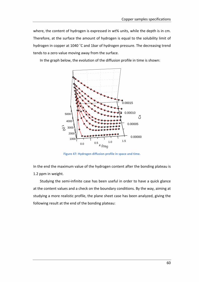
Copper samples specifications
60
where, the content of hydrogen is expressed in wt% units, while the depth is in cm.
Therefore, at the surface the amount of hydrogen is equal to the solubility limit of
hydrogen in copper at 1040 ˚C and 1bar of hydrogen pressure. The decreasing trend
tends to a zero value moving away from the surface.
In the graph below, the evolution of the diffusion profile in time is shown:
Figure 47: Hydrogen diffusion profile in space and time.
In the end the maximum value of the hydrogen content after the bonding plateau is
1.2 ppm in weight.
Studying the semi‐infinite case has been useful in order to have a quick glance
at the content values and a check on the boundary conditions. By the way, aiming at
studying a more realistic profile, the plane sheet case has been analyzed, giving the
following result at the end of the bonding plateau:
0.0 0.5 1.0 1.51000
2000
3000
4000
5000
0.00000
0.00005
0.00010
0.00015
t (s)
Cx
x (cm)
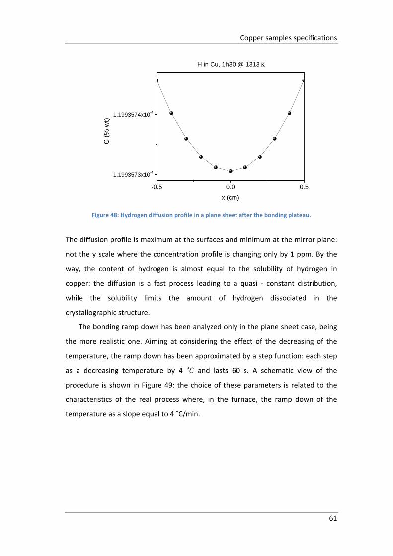
Copper samples specifications
61
Figure 48: Hydrogen diffusion profile in a plane sheet after the bonding plateau.
The diffusion profile is maximum at the surfaces and minimum at the mirror plane:
not the y scale where the concentration profile is changing only by 1 ppm. By the
way, the content of hydrogen is almost equal to the solubility of hydrogen in
copper: the diffusion is a fast process leading to a quasi ‐ constant distribution,
while the solubility limits the amount of hydrogen dissociated in the
crystallographic structure.
The bonding ramp down has been analyzed only in the plane sheet case, being
the more realistic one. Aiming at considering the effect of the decreasing of the
temperature, the ramp down has been approximated by a step function: each step
as a decreasing temperature by 4 ˚ and lasts 60 s. A schematic view of the
procedure is shown in Figure 49: the choice of these parameters is related to the
characteristics of the real process where, in the furnace, the ramp down of the
temperature as a slope equal to 4 ˚C/min.
-0.5 0.0 0.5
1.1993573x10⁻⁴
1.1993574x10⁻⁴
C (
% w
t)
x (cm)
H in Cu, 1h30 @ 1313
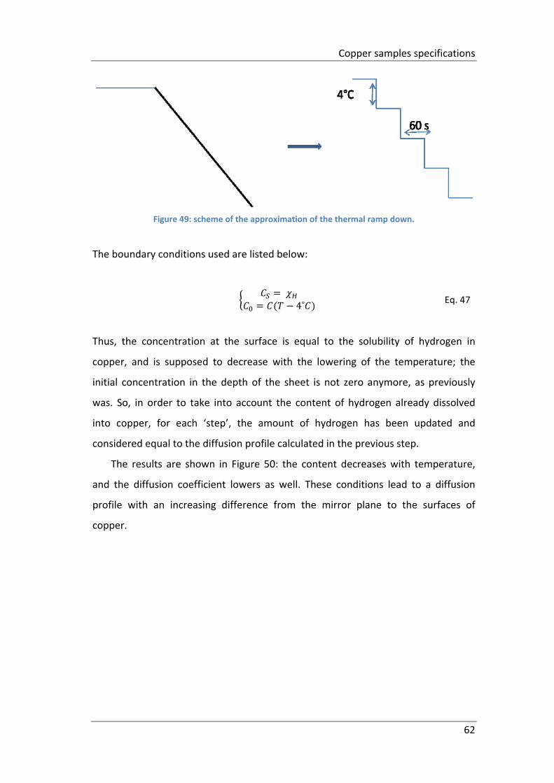
Copper samples specifications
62
Figure 49: scheme of the approximation of the thermal ramp down.
The boundary conditions used are listed below:
4˚
Eq. 47
Thus, the concentration at the surface is equal to the solubility of hydrogen in
copper, and is supposed to decrease with the lowering of the temperature; the
initial concentration in the depth of the sheet is not zero anymore, as previously
was. So, in order to take into account the content of hydrogen already dissolved
into copper, for each ‘step’, the amount of hydrogen has been updated and
considered equal to the diffusion profile calculated in the previous step.
The results are shown in Figure 50: the content decreases with temperature,
and the diffusion coefficient lowers as well. These conditions lead to a diffusion
profile with an increasing difference from the mirror plane to the surfaces of
copper.
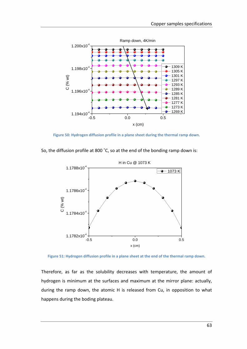
Copper samples specifications
63
Figure 50: Hydrogen diffusion profile in a plane sheet during the thermal ramp down.
So, the diffusion profile at 800 ˚C, so at the end of the bonding ramp down is:
Figure 51: Hydrogen diffusion profile in a plane sheet at the end of the thermal ramp down.
Therefore, as far as the solubility decreases with temperature, the amount of
hydrogen is minimum at the surfaces and maximum at the mirror plane: actually,
during the ramp down, the atomic H is released from Cu, in opposition to what
happens during the boding plateau.
-0.5 0.0 0.51.194x10-4
1.196x10⁻⁴
1.198x10⁻⁴
1.200x10⁻⁴
C (
% w
t)
x (cm)
1309 K 1305 K 1301 K 1297 K 1293 K 1289 K 1285 K 1281 K 1277 K 1273 K 1269 K
Ramp down, 4K/min
-0.5 0.0 0.51.1782x10-4
1.1784x10⁻⁴
1.1786x10⁻⁴
1.1788x10⁻⁴
C (
% w
t)
x (cm)
1073 K
H in Cu @ 1073 K
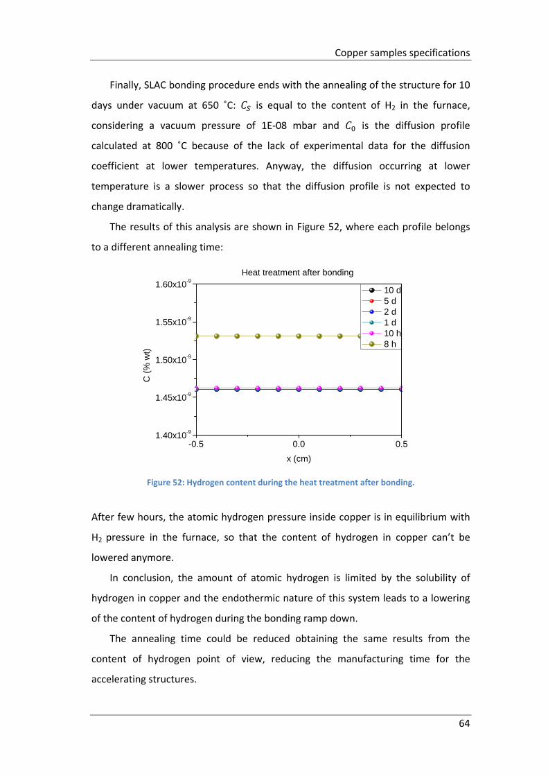
Copper samples specifications
64
Finally, SLAC bonding procedure ends with the annealing of the structure for 10
days under vacuum at 650 ˚C: is equal to the content of H2 in the furnace,
considering a vacuum pressure of 1E‐08 mbar and is the diffusion profile
calculated at 800 ˚C because of the lack of experimental data for the diffusion
coefficient at lower temperatures. Anyway, the diffusion occurring at lower
temperature is a slower process so that the diffusion profile is not expected to
change dramatically.
The results of this analysis are shown in Figure 52, where each profile belongs
to a different annealing time:
Figure 52: Hydrogen content during the heat treatment after bonding.
After few hours, the atomic hydrogen pressure inside copper is in equilibrium with
H2 pressure in the furnace, so that the content of hydrogen in copper can’t be
lowered anymore.
In conclusion, the amount of atomic hydrogen is limited by the solubility of
hydrogen in copper and the endothermic nature of this system leads to a lowering
of the content of hydrogen during the bonding ramp down.
The annealing time could be reduced obtaining the same results from the
content of hydrogen point of view, reducing the manufacturing time for the
accelerating structures.
-0.5 0.0 0.51.40x10-9
1.45x10⁻⁹
1.50x10⁻⁹
1.55x10⁻⁹
1.60x10⁻⁹
C (
% w
t)
x (cm)
10 d 5 d 2 d 1 d 10 h 8 h
Heat treatment after bonding
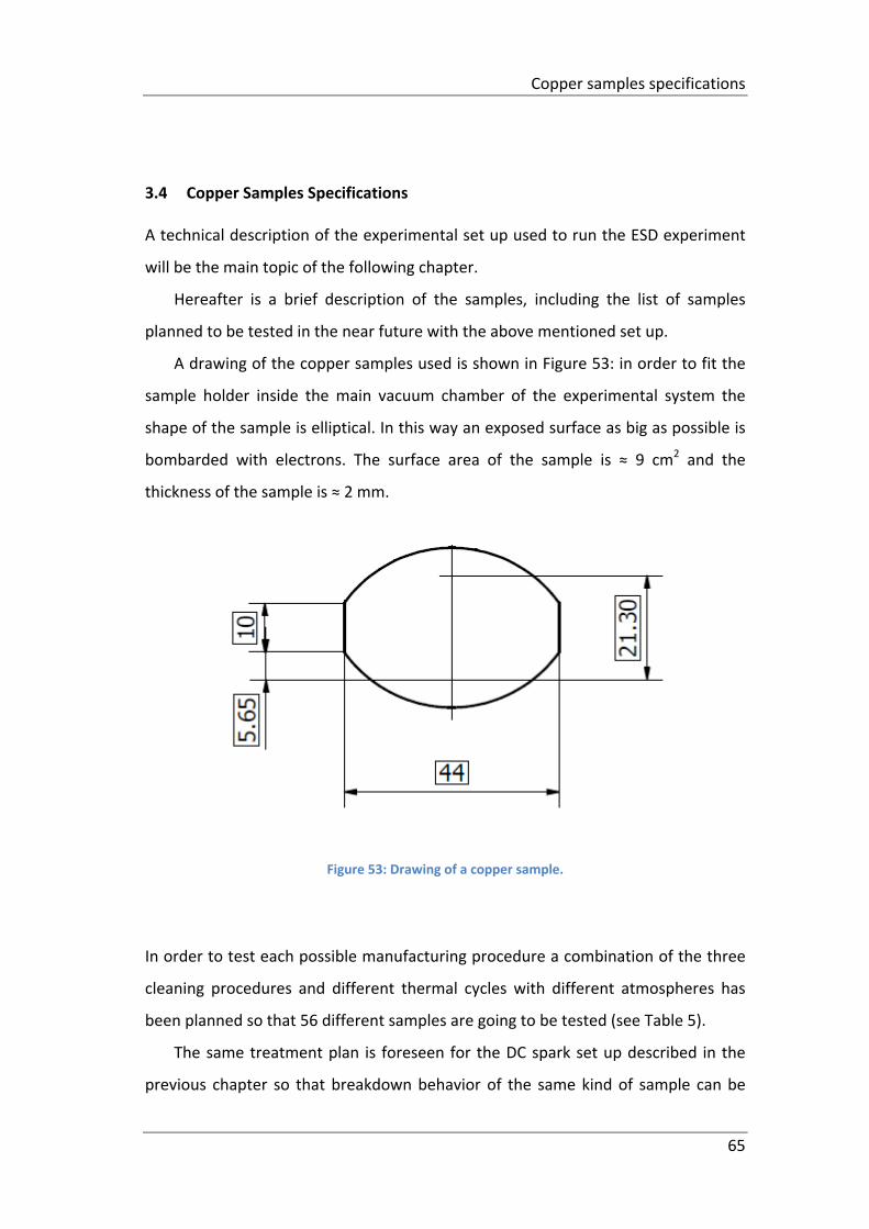
Copper samples specifications
65
3.4 Copper Samples Specifications
A technical description of the experimental set up used to run the ESD experiment
will be the main topic of the following chapter.
Hereafter is a brief description of the samples, including the list of samples
planned to be tested in the near future with the above mentioned set up.
A drawing of the copper samples used is shown in Figure 53: in order to fit the
sample holder inside the main vacuum chamber of the experimental system the
shape of the sample is elliptical. In this way an exposed surface as big as possible is
bombarded with electrons. The surface area of the sample is ≈ 9 cm2 and the
thickness of the sample is ≈ 2 mm.
Figure 53: Drawing of a copper sample.
In order to test each possible manufacturing procedure a combination of the three
cleaning procedures and different thermal cycles with different atmospheres has
been planned so that 56 different samples are going to be tested (see Table 5).
The same treatment plan is foreseen for the DC spark set up described in the
previous chapter so that breakdown behavior of the same kind of sample can be
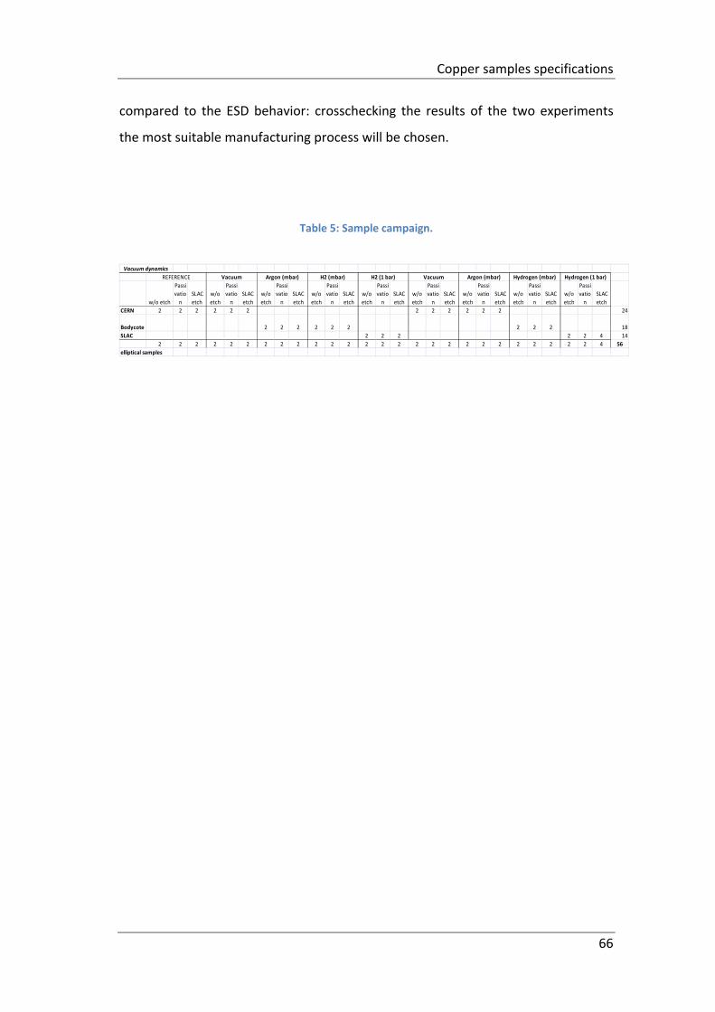
Copper samples specifications
66
compared to the ESD behavior: crosschecking the results of the two experiments
the most suitable manufacturing process will be chosen.
Table 5: Sample campaign.
w/o etch
Passi
vatio
n
SLAC
etch
w/o
etch
Passi
vatio
n
SLAC
etch
w/o
etch
Passi
vatio
n
SLAC
etch
w/o
etch
Passi
vatio
n
SLAC
etch
w/o
etch
Passi
vatio
n
SLAC
etch
w/o
etch
Passi
vatio
n
SLAC
etch
w/o
etch
Passi
vatio
n
SLAC
etch
w/o
etch
Passi
vatio
n
SLAC
etch
w/o
etch
Passi
vatio
n
SLAC
etch
CERN 2 2 2 2 2 2 2 2 2 2 2 2 24
Bodycote 2 2 2 2 2 2 2 2 2 18
SLAC 2 2 2 2 2 4 14
2 2 2 2 2 2 2 2 2 2 2 2 2 2 2 2 2 2 2 2 2 2 2 2 2 2 4 56
Hydrogen (1 bar)
elliptical samples
Vacuum dynamics
REFERENCE Vacuum Argon (mbar) H2 (mbar) H2 (1 bar) Vacuum Argon (mbar) Hydrogen (mbar)
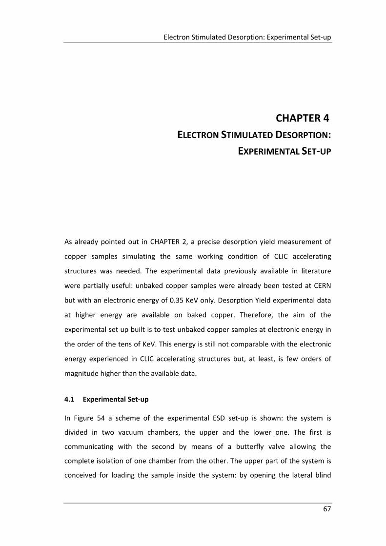
Electron Stimulated Desorption: Experimental Set‐up
67
CHAPTER 4
ELECTRON STIMULATED DESORPTION:
EXPERIMENTAL SET‐UP
As already pointed out in CHAPTER 2, a precise desorption yield measurement of
copper samples simulating the same working condition of CLIC accelerating
structures was needed. The experimental data previously available in literature
were partially useful: unbaked copper samples were already been tested at CERN
but with an electronic energy of 0.35 KeV only. Desorption Yield experimental data
at higher energy are available on baked copper. Therefore, the aim of the
experimental set up built is to test unbaked copper samples at electronic energy in
the order of the tens of KeV. This energy is still not comparable with the electronic
energy experienced in CLIC accelerating structures but, at least, is few orders of
magnitude higher than the available data.
4.1 Experimental Set‐up
In Figure 54 a scheme of the experimental ESD set‐up is shown: the system is
divided in two vacuum chambers, the upper and the lower one. The first is
communicating with the second by means of a butterfly valve allowing the
complete isolation of one chamber from the other. The upper part of the system is
conceived for loading the sample inside the system: by opening the lateral blind
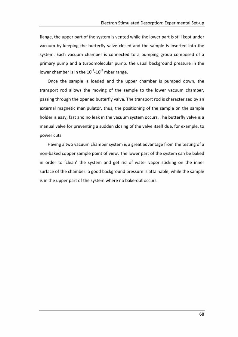
Electron Stimulated Desorption: Experimental Set‐up
68
flange, the upper part of the system is vented while the lower part is still kept under
vacuum by keeping the butterfly valve closed and the sample is inserted into the
system. Each vacuum chamber is connected to a pumping group composed of a
primary pump and a turbomolecular pump: the usual background pressure in the
lower chamber is in the 10‐8‐10‐9 mbar range.
Once the sample is loaded and the upper chamber is pumped down, the
transport rod allows the moving of the sample to the lower vacuum chamber,
passing through the opened butterfly valve. The transport rod is characterized by an
external magnetic manipulator, thus, the positioning of the sample on the sample
holder is easy, fast and no leak in the vacuum system occurs. The butterfly valve is a
manual valve for preventing a sudden closing of the valve itself due, for example, to
power cuts.
Having a two vacuum chamber system is a great advantage from the testing of a
non‐baked copper sample point of view. The lower part of the system can be baked
in order to ‘clean’ the system and get rid of water vapor sticking on the inner
surface of the chamber: a good background pressure is attainable, while the sample
is in the upper part of the system where no bake‐out occurs.
Electron Stimulated Desorption: Experimental Set‐up
69
Figure 54: ESD system experimental set‐ up.
Figure 55: insight of the experimental set – up: lower and upper vacuum chamber.
Electron Stimulated Desorption: Experimental Set‐up
70
A tungsten filament is the electron source for bombarding the sample which can be
positively polarized in the 0 – 20 KV range. Actually, the FUG power supply could
operate up to 35 KV but the voltage is limited by the vacuum electrical power
feedthrough.
The typical operating values for the filament are: 2‐3 A, 4‐9 W and is positively
biased to the ground at +15 V.
The electrical circuit of the system is shown in Figure 56: two electrometers are
connected to the circuit so that, the one connected to the filament reads the
current of electrons emitted due to the thermoionic effect, while, the second one
connected to the power feedthrough reads the electronic current impinging on the
sample. Therefore, if no other electron sources are in the system, the two currents
read with the two instruments should be the same and the electrical circuit is closed
by the electrons emitted from the filament and accelerated toward the sample.
Finally, the filament is slightly positively biased to the ground in order to
prevent the worsening of the background pressure: the electrons emitted when the
sample is not biased are attracted by the filament itself so that no desorption effect
coming from the inner surfaces of the vacuum chamber occurs.
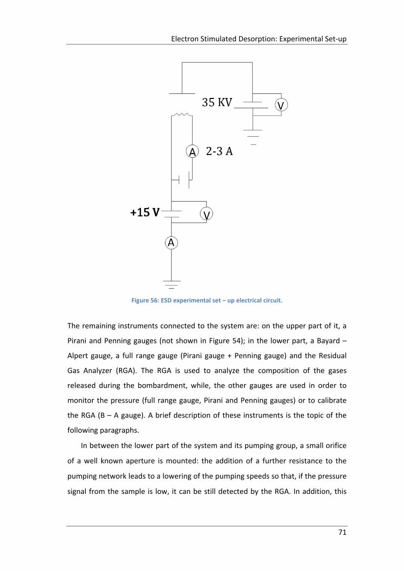
Electron Stimulated Desorption: Experimental Set‐up
71
Figure 56: ESD experimental set – up electrical circuit.
The remaining instruments connected to the system are: on the upper part of it, a
Pirani and Penning gauges (not shown in Figure 54); in the lower part, a Bayard –
Alpert gauge, a full range gauge (Pirani gauge + Penning gauge) and the Residual
Gas Analyzer (RGA). The RGA is used to analyze the composition of the gases
released during the bombardment, while, the other gauges are used in order to
monitor the pressure (full range gauge, Pirani and Penning gauges) or to calibrate
the RGA (B – A gauge). A brief description of these instruments is the topic of the
following paragraphs.
In between the lower part of the system and its pumping group, a small orifice
of a well known aperture is mounted: the addition of a further resistance to the
pumping network leads to a lowering of the pumping speeds so that, if the pressure
signal from the sample is low, it can be still detected by the RGA. In addition, this
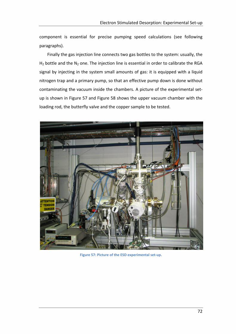
Electron Stimulated Desorption: Experimental Set‐up
72
component is essential for precise pumping speed calculations (see following
paragraphs).
Finally the gas injection line connects two gas bottles to the system: usually, the
H2 bottle and the N2 one. The injection line is essential in order to calibrate the RGA
signal by injecting in the system small amounts of gas: it is equipped with a liquid
nitrogen trap and a primary pump, so that an effective pump down is done without
contaminating the vacuum inside the chambers. A picture of the experimental set‐
up is shown in Figure 57 and Figure 58 shows the upper vacuum chamber with the
loading rod, the butterfly valve and the copper sample to be tested.
Figure 57: Picture of the ESD experimental set‐up.
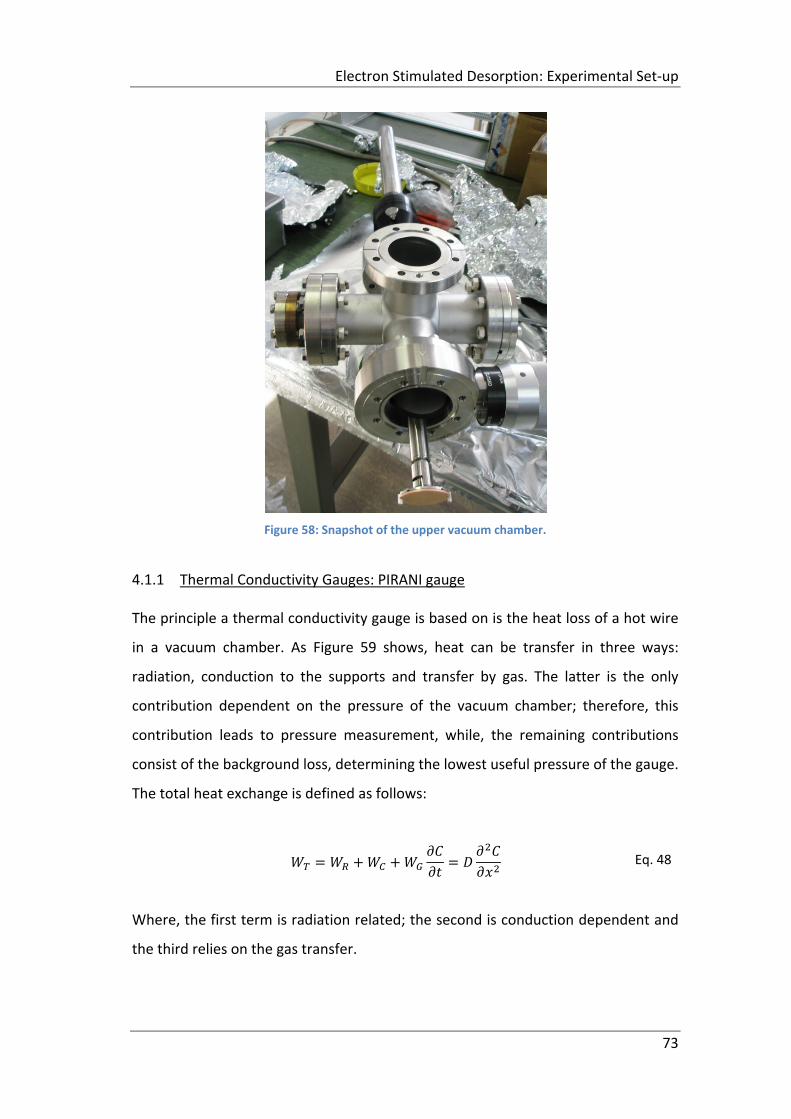
Electron Stimulated Desorption: Experimental Set‐up
73
Figure 58: Snapshot of the upper vacuum chamber.
4.1.1 Thermal Conductivity Gauges: PIRANI gauge
The principle a thermal conductivity gauge is based on is the heat loss of a hot wire
in a vacuum chamber. As Figure 59 shows, heat can be transfer in three ways:
radiation, conduction to the supports and transfer by gas. The latter is the only
contribution dependent on the pressure of the vacuum chamber; therefore, this
contribution leads to pressure measurement, while, the remaining contributions
consist of the background loss, determining the lowest useful pressure of the gauge.
The total heat exchange is defined as follows:
Eq. 48
Where, the first term is radiation related; the second is conduction dependent and
the third relies on the gas transfer.
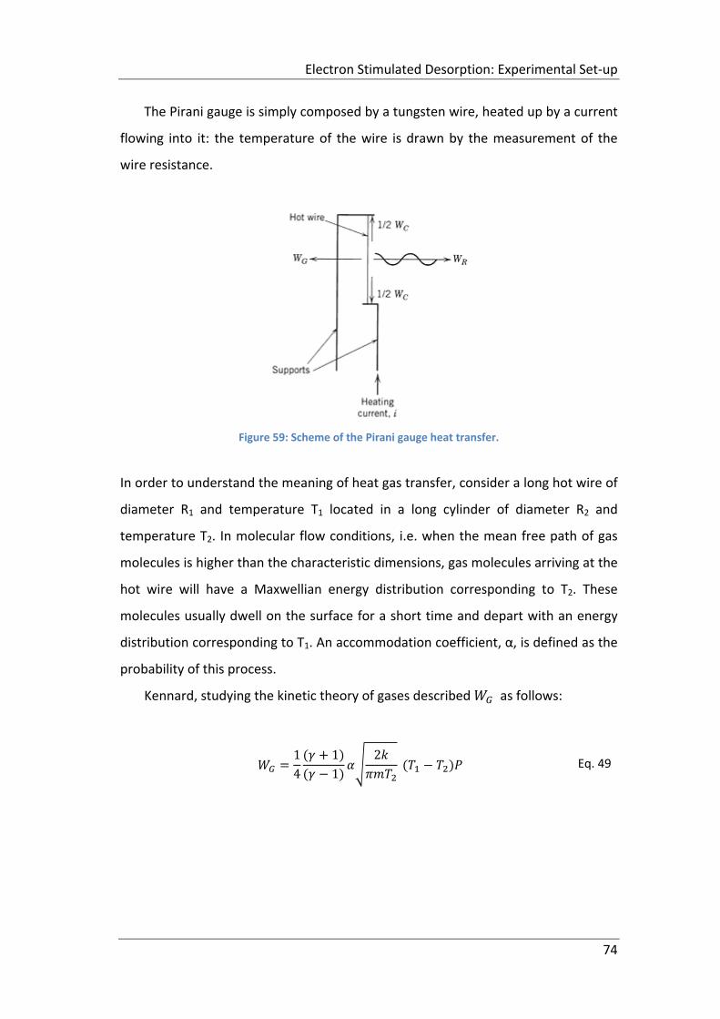
Electron Stimulated Desorption: Experimental Set‐up
74
The Pirani gauge is simply composed by a tungsten wire, heated up by a current
flowing into it: the temperature of the wire is drawn by the measurement of the
wire resistance.
Figure 59: Scheme of the Pirani gauge heat transfer.
In order to understand the meaning of heat gas transfer, consider a long hot wire of
diameter R1 and temperature T1 located in a long cylinder of diameter R2 and
temperature T2. In molecular flow conditions, i.e. when the mean free path of gas
molecules is higher than the characteristic dimensions, gas molecules arriving at the
hot wire will have a Maxwellian energy distribution corresponding to T2. These
molecules usually dwell on the surface for a short time and depart with an energy
distribution corresponding to T1. An accommodation coefficient, α, is defined as the
probability of this process.
Kennard, studying the kinetic theory of gases described as follows:
1
4
1
1
2 Eq. 49
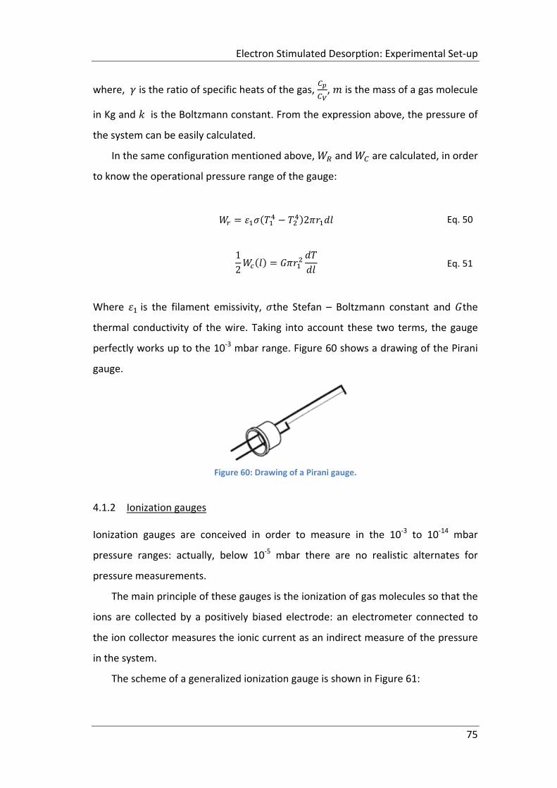
Electron Stimulated Desorption: Experimental Set‐up
75
where, is the ratio of specific heats of the gas, , is the mass of a gas molecule
in Kg and is the Boltzmann constant. From the expression above, the pressure of
the system can be easily calculated.
In the same configuration mentioned above, and are calculated, in order
to know the operational pressure range of the gauge:
2 Eq. 50
1
2 Eq. 51
Where is the filament emissivity, the Stefan – Boltzmann constant and the
thermal conductivity of the wire. Taking into account these two terms, the gauge
perfectly works up to the 10‐3 mbar range. Figure 60 shows a drawing of the Pirani
gauge.
Figure 60: Drawing of a Pirani gauge.
4.1.2 Ionization gauges
Ionization gauges are conceived in order to measure in the 10‐3 to 10‐14 mbar
pressure ranges: actually, below 10‐5 mbar there are no realistic alternates for
pressure measurements.
The main principle of these gauges is the ionization of gas molecules so that the
ions are collected by a positively biased electrode: an electrometer connected to
the ion collector measures the ionic current as an indirect measure of the pressure
in the system.
The scheme of a generalized ionization gauge is shown in Figure 61:
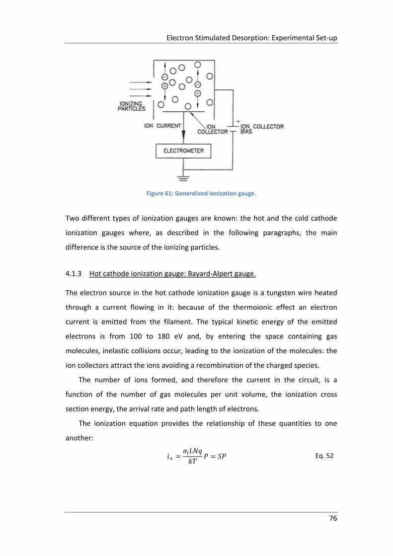
Electron Stimulated Desorption: Experimental Set‐up
76
Figure 61: Generalized ionization gauge.
Two different types of ionization gauges are known: the hot and the cold cathode
ionization gauges where, as described in the following paragraphs, the main
difference is the source of the ionizing particles.
4.1.3 Hot cathode ionization gauge: Bayard‐Alpert gauge.
The electron source in the hot cathode ionization gauge is a tungsten wire heated
through a current flowing in it: because of the thermoionic effect an electron
current is emitted from the filament. The typical kinetic energy of the emitted
electrons is from 100 to 180 eV and, by entering the space containing gas
molecules, inelastic collisions occur, leading to the ionization of the molecules: the
ion collectors attract the ions avoiding a recombination of the charged species.
The number of ions formed, and therefore the current in the circuit, is a
function of the number of gas molecules per unit volume, the ionization cross
section energy, the arrival rate and path length of electrons.
The ionization equation provides the relationship of these quantities to one
another:
Eq. 52
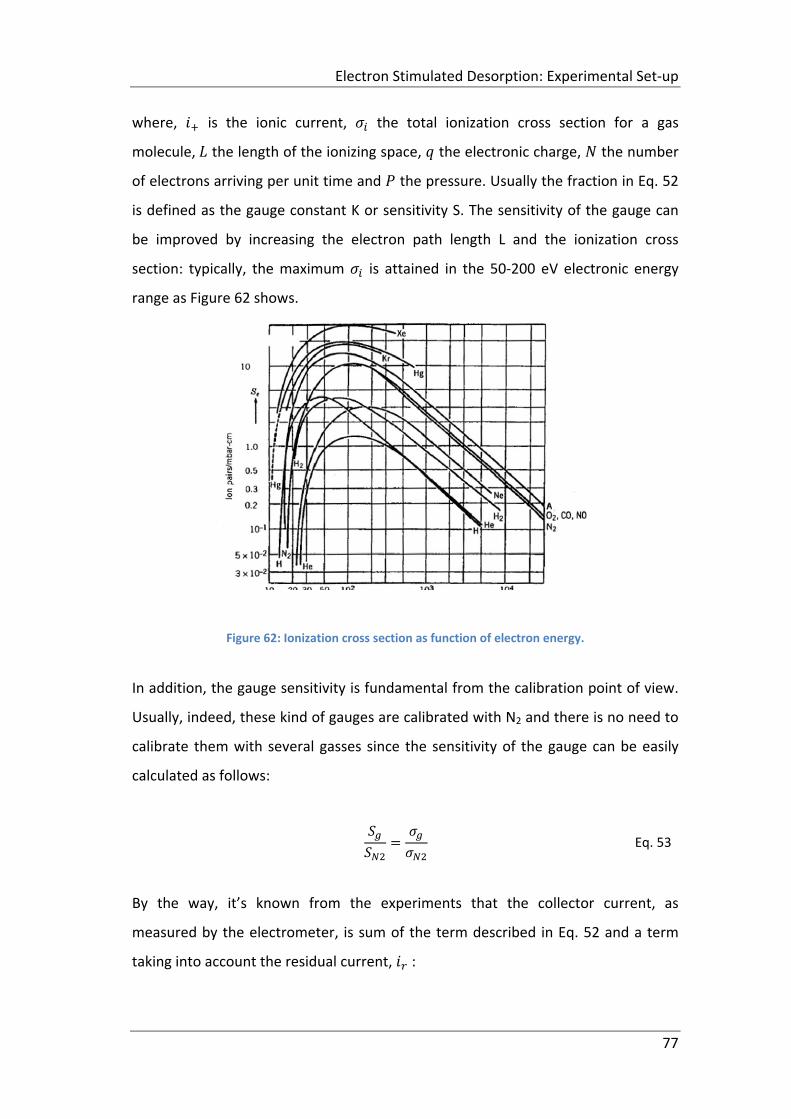
Electron Stimulated Desorption: Experimental Set‐up
77
where, is the ionic current, the total ionization cross section for a gas
molecule, the length of the ionizing space, the electronic charge, the number
of electrons arriving per unit time and the pressure. Usually the fraction in Eq. 52
is defined as the gauge constant K or sensitivity S. The sensitivity of the gauge can
be improved by increasing the electron path length L and the ionization cross
section: typically, the maximum is attained in the 50‐200 eV electronic energy
range as Figure 62 shows.
Figure 62: Ionization cross section as function of electron energy.
In addition, the gauge sensitivity is fundamental from the calibration point of view.
Usually, indeed, these kind of gauges are calibrated with N2 and there is no need to
calibrate them with several gasses since the sensitivity of the gauge can be easily
calculated as follows:
Eq. 53
By the way, it’s known from the experiments that the collector current, as
measured by the electrometer, is sum of the term described in Eq. 52 and a term
taking into account the residual current, :
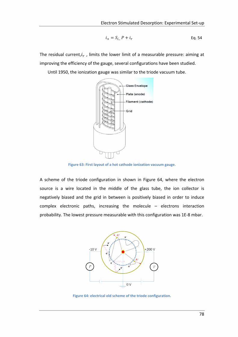
Electron Stimulated Desorption: Experimental Set‐up
78
Eq. 54
The residual current, , limits the lower limit of a measurable pressure: aiming at
improving the efficiency of the gauge, several configurations have been studied.
Until 1950, the ionization gauge was similar to the triode vacuum tube.
Figure 63: First layout of a hot cathode ionization vacuum gauge.
A scheme of the triode configuration in shown in Figure 64, where the electron
source is a wire located in the middle of the glass tube, the ion collector is
negatively biased and the grid in between is positively biased in order to induce
complex electronic paths, increasing the molecule – electrons interaction
probability. The lowest pressure measurable with this configuration was 1E‐8 mbar.
Figure 64: electrical old scheme of the triode configuration.
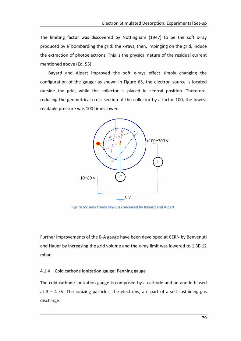
Electron Stimulated Desorption: Experimental Set‐up
79
The limiting factor was discovered by Nottingham (1947) to be the soft x‐ray
produced by e‐ bombarding the grid: the x‐rays, then, impinging on the grid, induce
the extraction of photoelectrons. This is the physical nature of the residual current
mentioned above (Eq. 55).
Bayard and Alpert improved the soft x‐rays effect simply changing the
configuration of the gauge: as shown in Figure 65, the electron source is located
outside the grid, while the collector is placed in central position. Therefore,
reducing the geometrical cross section of the collector by a factor 100, the lowest
readable pressure was 100 times lower.
Figure 65: new triode lay‐out conceived by Bayard and Alpert.
Further improvements of the B‐A gauge have been developed at CERN by Benvenuti
and Hauer by increasing the grid volume and the x‐ray limit was lowered to 1.3E‐12
mbar.
4.1.4 Cold cathode ionization gauge: Penning gauge
The cold cathode ionization gauge is composed by a cathode and an anode biased
at 3 – 4 kV. The ionizing particles, the electrons, are part of a self‐sustaining gas
discharge.
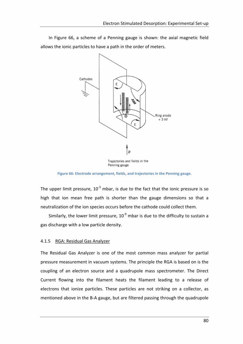
Electron Stimulated Desorption: Experimental Set‐up
80
In Figure 66, a scheme of a Penning gauge is shown: the axial magnetic field
allows the ionic particles to have a path in the order of meters.
Figure 66: Electrode arrangement, fields, and trajectories in the Penning gauge.
The upper limit pressure, 10‐3 mbar, is due to the fact that the ionic pressure is so
high that ion mean free path is shorter than the gauge dimensions so that a
neutralization of the ion species occurs before the cathode could collect them.
Similarly, the lower limit pressure, 10‐9 mbar is due to the difficulty to sustain a
gas discharge with a low particle density.
4.1.5 RGA: Residual Gas Analyzer
The Residual Gas Analyzer is one of the most common mass analyzer for partial
pressure measurement in vacuum systems. The principle the RGA is based on is the
coupling of an electron source and a quadrupole mass spectrometer. The Direct
Current flowing into the filament heats the filament leading to a release of
electrons that ionize particles. These particles are not striking on a collector, as
mentioned above in the B‐A gauge, but are filtered passing through the quadrupole
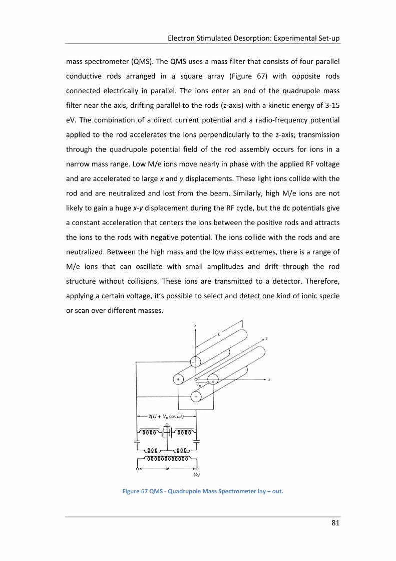
Electron Stimulated Desorption: Experimental Set‐up
81
mass spectrometer (QMS). The QMS uses a mass filter that consists of four parallel
conductive rods arranged in a square array (Figure 67) with opposite rods
connected electrically in parallel. The ions enter an end of the quadrupole mass
filter near the axis, drifting parallel to the rods (z‐axis) with a kinetic energy of 3‐15
eV. The combination of a direct current potential and a radio‐frequency potential
applied to the rod accelerates the ions perpendicularly to the z‐axis; transmission
through the quadrupole potential field of the rod assembly occurs for ions in a
narrow mass range. Low M/e ions move nearly in phase with the applied RF voltage
and are accelerated to large x and y displacements. These light ions collide with the
rod and are neutralized and lost from the beam. Similarly, high M/e ions are not
likely to gain a huge x‐y displacement during the RF cycle, but the dc potentials give
a constant acceleration that centers the ions between the positive rods and attracts
the ions to the rods with negative potential. The ions collide with the rods and are
neutralized. Between the high mass and the low mass extremes, there is a range of
M/e ions that can oscillate with small amplitudes and drift through the rod
structure without collisions. These ions are transmitted to a detector. Therefore,
applying a certain voltage, it’s possible to select and detect one kind of ionic specie
or scan over different masses.
Figure 67 QMS ‐ Quadrupole Mass Spectrometer lay – out.
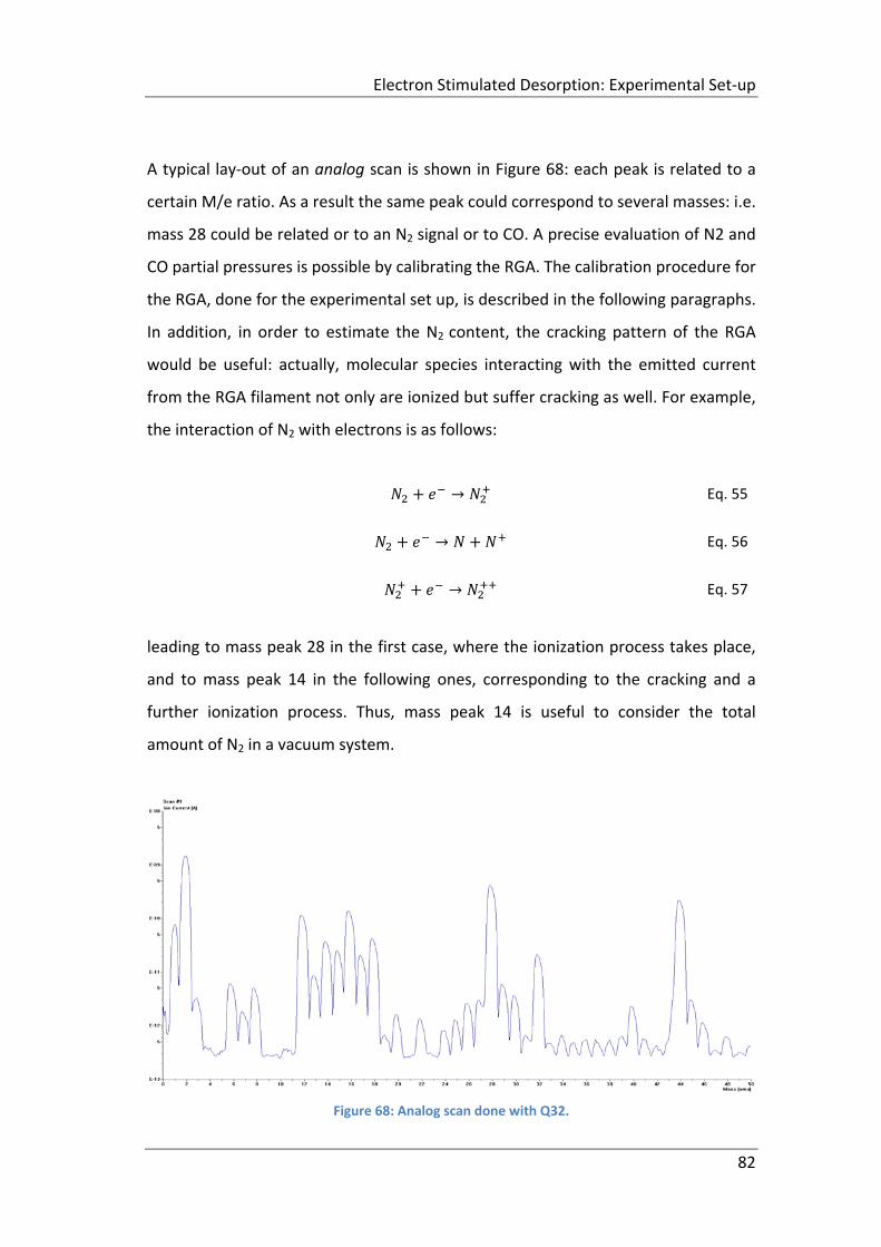
Electron Stimulated Desorption: Experimental Set‐up
82
A typical lay‐out of an analog scan is shown in Figure 68: each peak is related to a
certain M/e ratio. As a result the same peak could correspond to several masses: i.e.
mass 28 could be related or to an N2 signal or to CO. A precise evaluation of N2 and
CO partial pressures is possible by calibrating the RGA. The calibration procedure for
the RGA, done for the experimental set up, is described in the following paragraphs.
In addition, in order to estimate the N2 content, the cracking pattern of the RGA
would be useful: actually, molecular species interacting with the emitted current
from the RGA filament not only are ionized but suffer cracking as well. For example,
the interaction of N2 with electrons is as follows:
→ Eq. 55
→ Eq. 56
→ Eq. 57
leading to mass peak 28 in the first case, where the ionization process takes place,
and to mass peak 14 in the following ones, corresponding to the cracking and a
further ionization process. Thus, mass peak 14 is useful to consider the total
amount of N2 in a vacuum system.
Figure 68: Analog scan done with Q32.
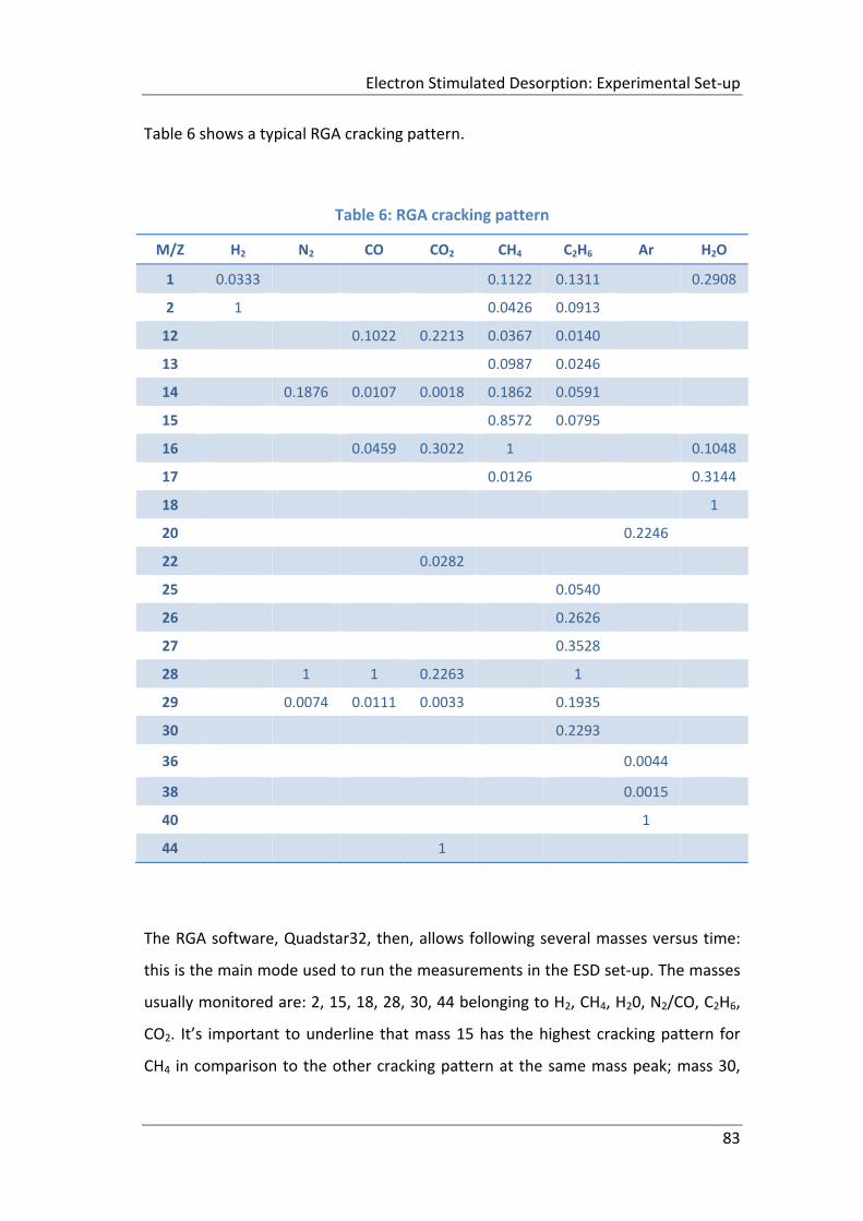
Electron Stimulated Desorption: Experimental Set‐up
83
Table 6 shows a typical RGA cracking pattern.
Table 6: RGA cracking pattern
M/Z H2 N2 CO CO2 CH4 C2H6 Ar H2O
1 0.0333 0.1122 0.1311 0.2908
2 1 0.0426 0.0913
12 0.1022 0.2213 0.0367 0.0140
13 0.0987 0.0246
14 0.1876 0.0107 0.0018 0.1862 0.0591
15 0.8572 0.0795
16 0.0459 0.3022 1 0.1048
17 0.0126 0.3144
18 1
20 0.2246
22 0.0282
25 0.0540
26 0.2626
27 0.3528
28 1 1 0.2263 1
29 0.0074 0.0111 0.0033 0.1935
30 0.2293
36 0.0044
38 0.0015
40 1
44 1
The RGA software, Quadstar32, then, allows following several masses versus time:
this is the main mode used to run the measurements in the ESD set‐up. The masses
usually monitored are: 2, 15, 18, 28, 30, 44 belonging to H2, CH4, H20, N2/CO, C2H6,
CO2. It’s important to underline that mass 15 has the highest cracking pattern for
CH4 in comparison to the other cracking pattern at the same mass peak; mass 30,
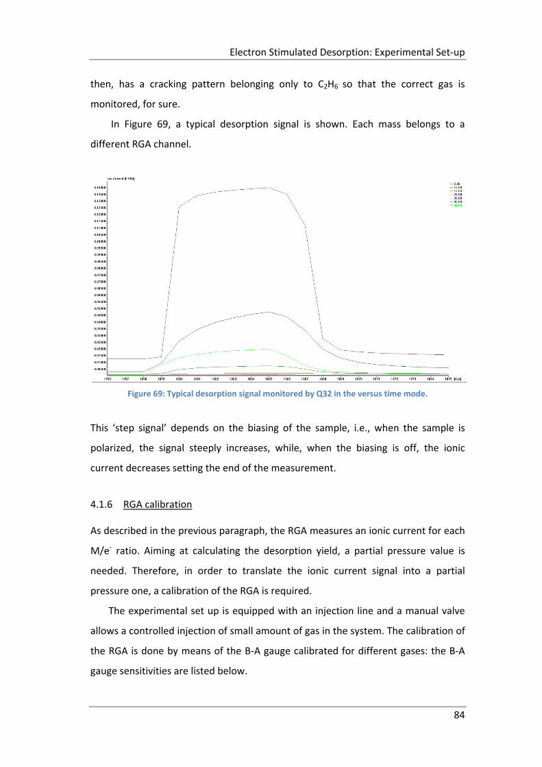
Electron Stimulated Desorption: Experimental Set‐up
84
then, has a cracking pattern belonging only to C2H6 so that the correct gas is
monitored, for sure.
In Figure 69, a typical desorption signal is shown. Each mass belongs to a
different RGA channel.
Figure 69: Typical desorption signal monitored by Q32 in the versus time mode.
This ‘step signal’ depends on the biasing of the sample, i.e., when the sample is
polarized, the signal steeply increases, while, when the biasing is off, the ionic
current decreases setting the end of the measurement.
4.1.6 RGA calibration
As described in the previous paragraph, the RGA measures an ionic current for each
M/e‐ ratio. Aiming at calculating the desorption yield, a partial pressure value is
needed. Therefore, in order to translate the ionic current signal into a partial
pressure one, a calibration of the RGA is required.
The experimental set up is equipped with an injection line and a manual valve
allows a controlled injection of small amount of gas in the system. The calibration of
the RGA is done by means of the B‐A gauge calibrated for different gases: the B‐A
gauge sensitivities are listed below.
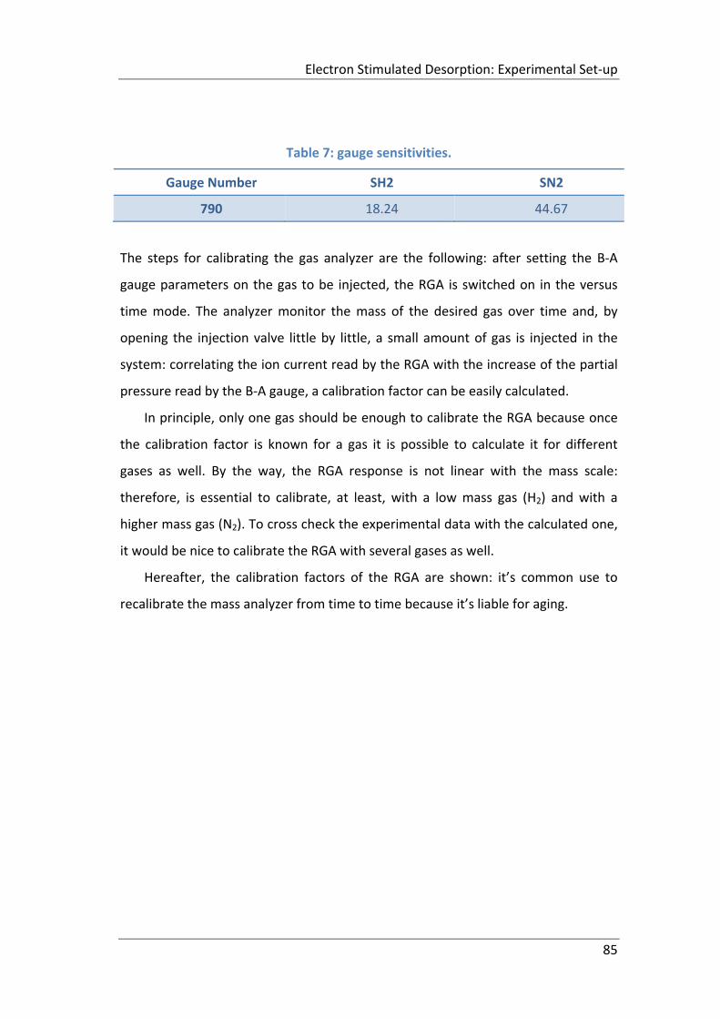
Electron Stimulated Desorption: Experimental Set‐up
85
Table 7: gauge sensitivities.
Gauge Number SH2 SN2
790 18.24 44.67
The steps for calibrating the gas analyzer are the following: after setting the B‐A
gauge parameters on the gas to be injected, the RGA is switched on in the versus
time mode. The analyzer monitor the mass of the desired gas over time and, by
opening the injection valve little by little, a small amount of gas is injected in the
system: correlating the ion current read by the RGA with the increase of the partial
pressure read by the B‐A gauge, a calibration factor can be easily calculated.
In principle, only one gas should be enough to calibrate the RGA because once
the calibration factor is known for a gas it is possible to calculate it for different
gases as well. By the way, the RGA response is not linear with the mass scale:
therefore, is essential to calibrate, at least, with a low mass gas (H2) and with a
higher mass gas (N2). To cross check the experimental data with the calculated one,
it would be nice to calibrate the RGA with several gases as well.
Hereafter, the calibration factors of the RGA are shown: it’s common use to
recalibrate the mass analyzer from time to time because it’s liable for aging.
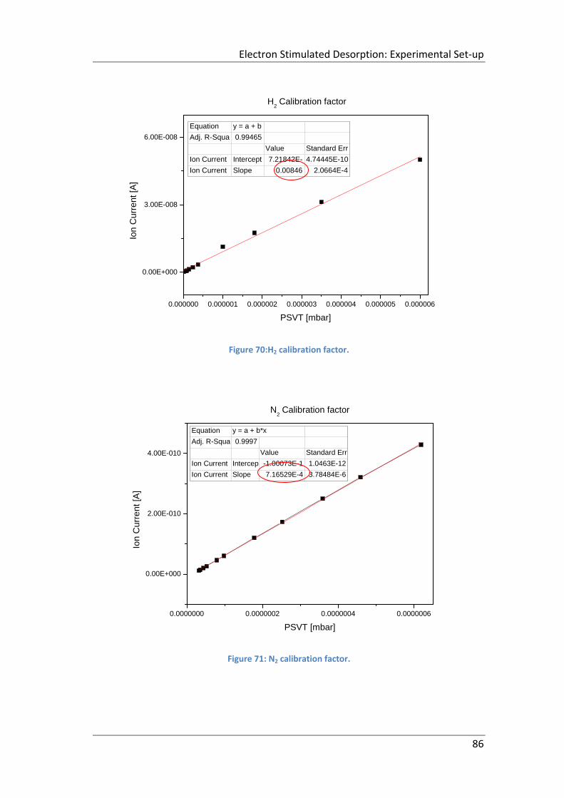
Electron Stimulated Desorption: Experimental Set‐up
86
Figure 70:H2 calibration factor.
Figure 71: N2 calibration factor.
0.0000000 0.0000002 0.0000004 0.0000006
0.00E+000
2.00E-010
4.00E-010
Ion
Cu
rre
nt [A
]
PSVT [mbar]
Equation y = a + b*x
Adj. R-Squa 0.9997
Value Standard Err
Ion Current Intercep -1.00073E-1 1.0463E-12
Ion Current Slope 7.16529E-4 3.78484E-6
N2 Calibration factor
0.000000 0.000001 0.000002 0.000003 0.000004 0.000005 0.000006
0.00E+000
3.00E-008
6.00E-008Io
n C
urr
ent [
A]
PSVT [mbar]
Equation y = a + b
Adj. R-Squa 0.99465
Value Standard Err
Ion Current Intercept 7.21842E- 4.74445E-10
Ion Current Slope 0.00846 2.0664E-4
H2 Calibration factor
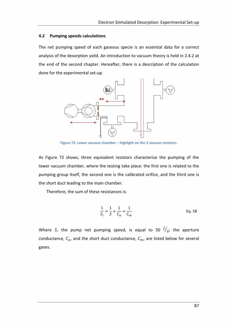
Electron Stimulated Desorption: Experimental Set‐up
87
4.2 Pumping speeds calculations
The net pumping speed of each gaseous specie is an essential data for a correct
analysis of the desorption yield. An introduction to vacuum theory is held in 2.4.2 at
the end of the second chapter. Hereafter, there is a description of the calculation
done for the experimental set‐up.
Figure 72: Lower vacuum chamber – highlight on the 3 vacuum resistors.
As Figure 72 shows, three equivalent resistors characterize the pumping of the
lower vacuum chamber, where the testing take place: the first one is related to the
pumping group itself, the second one is the calibrated orifice, and the third one is
the short duct leading to the main chamber.
Therefore, the sum of these resistances is:
1 1 1 1
Eq. 58
Where , the pump net pumping speed, is equal to 50 ; the aperture
conductance, , and the short duct conductance, , are listed below for several
gases.
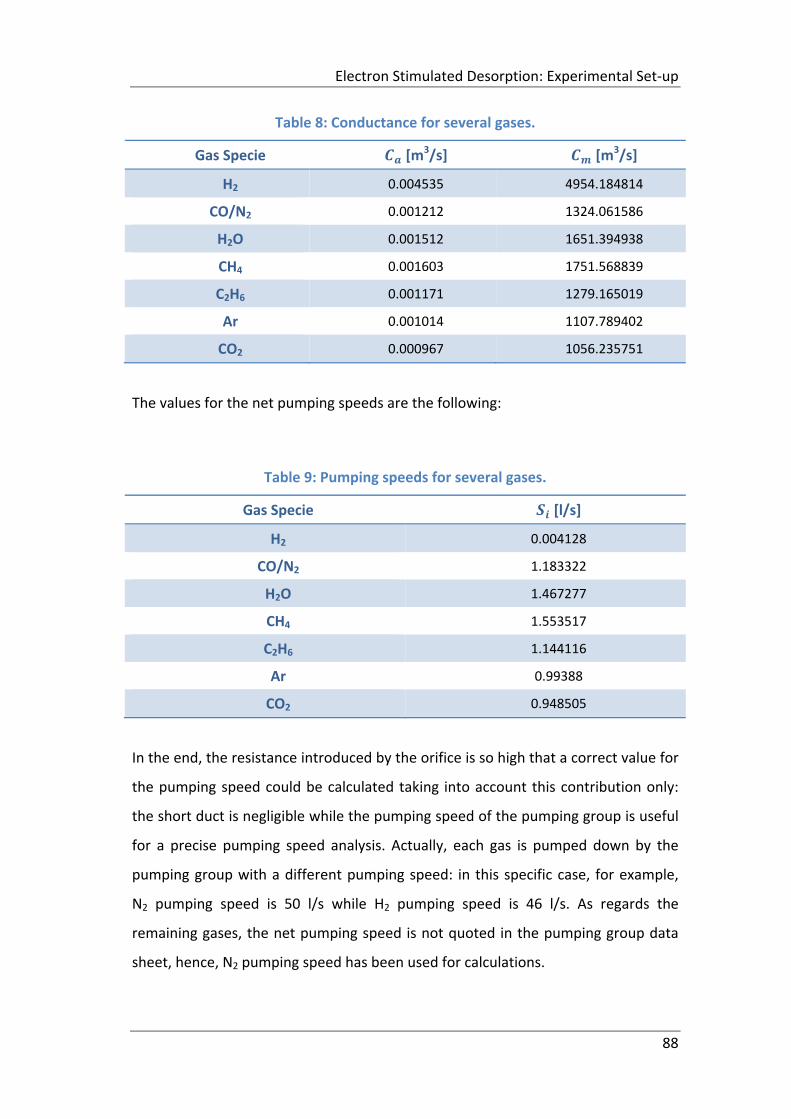
Electron Stimulated Desorption: Experimental Set‐up
88
Table 8: Conductance for several gases.
Gas Specie [m3/s] [m3/s]
H2 0.004535 4954.184814
CO/N2 0.001212 1324.061586
H2O 0.001512 1651.394938
CH4 0.001603 1751.568839
C2H6 0.001171 1279.165019
Ar 0.001014 1107.789402
CO2 0.000967 1056.235751
The values for the net pumping speeds are the following:
Table 9: Pumping speeds for several gases.
Gas Specie [l/s]
H2 0.004128
CO/N2 1.183322
H2O 1.467277
CH4 1.553517
C2H6 1.144116
Ar 0.99388
CO2 0.948505
In the end, the resistance introduced by the orifice is so high that a correct value for
the pumping speed could be calculated taking into account this contribution only:
the short duct is negligible while the pumping speed of the pumping group is useful
for a precise pumping speed analysis. Actually, each gas is pumped down by the
pumping group with a different pumping speed: in this specific case, for example,
N2 pumping speed is 50 l/s while H2 pumping speed is 46 l/s. As regards the
remaining gases, the net pumping speed is not quoted in the pumping group data
sheet, hence, N2 pumping speed has been used for calculations.
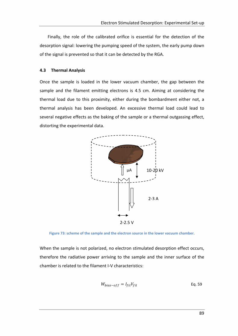
Electron Stimulated Desorption: Experimental Set‐up
89
Finally, the role of the calibrated orifice is essential for the detection of the
desorption signal: lowering the pumping speed of the system, the early pump down
of the signal is prevented so that it can be detected by the RGA.
4.3 Thermal Analysis
Once the sample is loaded in the lower vacuum chamber, the gap between the
sample and the filament emitting electrons is 4.5 cm. Aiming at considering the
thermal load due to this proximity, either during the bombardment either not, a
thermal analysis has been developed. An excessive thermal load could lead to
several negative effects as the baking of the sample or a thermal outgassing effect,
distorting the experimental data.
Figure 73: scheme of the sample and the electron source in the lower vacuum chamber.
When the sample is not polarized, no electron stimulated desorption effect occurs,
therefore the radiative power arriving to the sample and the inner surface of the
chamber is related to the filament I‐V characteristics:
Eq. 59
2‐3 A
2‐2.5 V
10‐20 kVµA
Electron Stimulated Desorption: Experimental Set‐up
90
In the specific case of the experimental set‐up is ~ 5 W.
If, then, the sample is positively biased and a current from the filament to the
sample flows, an additional contribution to the radiative power must be taken into
account:
Eq. 60
leading to a total released power of ~ 6 W.
This thermal power reaches the sample and the inner surface of the chamber
through radiation, since the system is operating in vacuum. Thus, the temperature
of the sample at the equilibrium is calculated from the radiation law for gray bodies:
Eq. 61
where, is the radiative power per surface unit; is the Stefan‐Boltzmann
constant, 5.67E‐8 ; , copper emissivity, 0.04, and , the
configuration factor taking into account the geometry of the system, 1.03E‐1. The
configuration factor is defined as follows:
Eq. 62
The meaning of each parameter is shown in picture in Figure 74:
]0175.0)1([*)1(*)1(
)1(*)1(*0152.13047.09767.1656.3195.1
4915.30251.1
2,1
DDBL
BLF
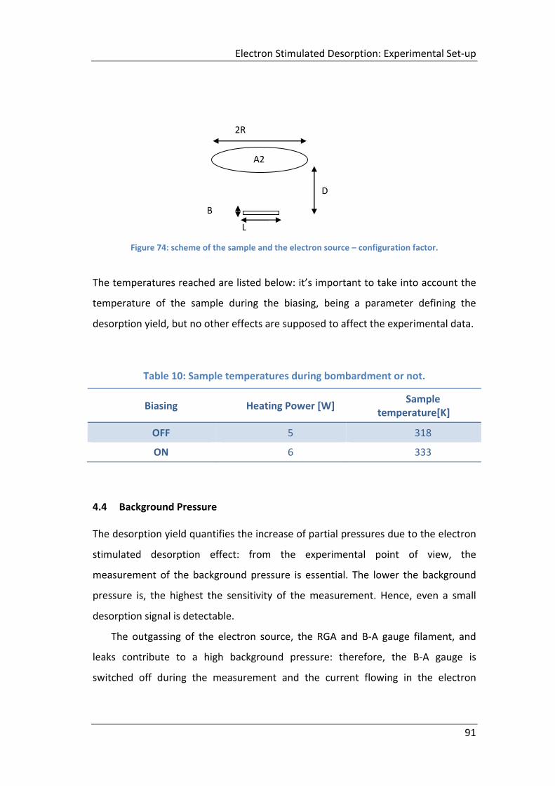
Electron Stimulated Desorption: Experimental Set‐up
91
Figure 74: scheme of the sample and the electron source – configuration factor.
The temperatures reached are listed below: it’s important to take into account the
temperature of the sample during the biasing, being a parameter defining the
desorption yield, but no other effects are supposed to affect the experimental data.
Table 10: Sample temperatures during bombardment or not.
Biasing Heating Power [W] Sample
temperature[K]
OFF 5 318
ON 6 333
4.4 Background Pressure
The desorption yield quantifies the increase of partial pressures due to the electron
stimulated desorption effect: from the experimental point of view, the
measurement of the background pressure is essential. The lower the background
pressure is, the highest the sensitivity of the measurement. Hence, even a small
desorption signal is detectable.
The outgassing of the electron source, the RGA and B‐A gauge filament, and
leaks contribute to a high background pressure: therefore, the B‐A gauge is
switched off during the measurement and the current flowing in the electron
D
L
B
2R
A2
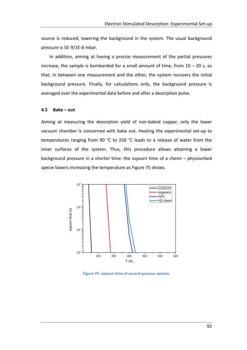
Electron Stimulated Desorption: Experimental Set‐up
92
source is reduced, lowering the background in the system. The usual background
pressure is 5E‐9/1E‐8 mbar.
In addition, aiming at having a precise measurement of the partial pressures
increase, the sample is bombarded for a small amount of time, from 10 – 20 s, so
that, in between one measurement and the other, the system recovers the initial
background pressure. Finally, for calculations only, the background pressure is
averaged over the experimental data before and after a desorption pulse.
4.5 Bake – out
Aiming at measuring the desorption yield of non‐baked copper, only the lower
vacuum chamber is concerned with bake out. Heating the experimental set‐up to
temperatures ranging from 90 °C to 250 °C leads to a release of water from the
inner surfaces of the system. Thus, this procedure allows attaining a lower
background pressure in a shorter time: the sojourn time of a chemi – physisorbed
specie lowers increasing the temperature as Figure 75 shows.
100 200 300 400 500 600100
101
102
103
sojo
urn
time
(s)
T (K)
CO/CO2 organics H20 H2 chem
Figure 75: sojourn time of several gaseous species.
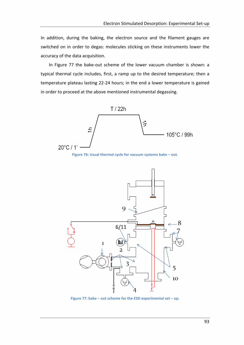
Electron Stimulated Desorption: Experimental Set‐up
93
In addition, during the baking, the electron source and the filament gauges are
switched on in order to degas: molecules sticking on these instruments lower the
accuracy of the data acquisition.
In Figure 77 the bake‐out scheme of the lower vacuum chamber is shown: a
typical thermal cycle includes, first, a ramp up to the desired temperature; then a
temperature plateau lasting 22‐24 hours; in the end a lower temperature is gained
in order to proceed at the above mentioned instrumental degassing.
Figure 76: Usual thermal cycle for vacuum systems bake – out.
Figure 77: bake – out scheme for the ESD experimental set – up.
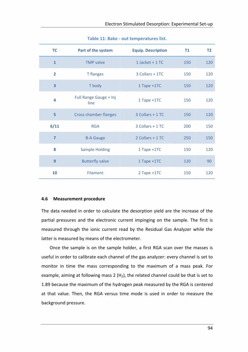
Electron Stimulated Desorption: Experimental Set‐up
94
Table 11: Bake ‐ out temperatures list.
TC Part of the system Equip. Description T1 T2
1 TMP valve 1 Jacket + 1 TC 150 120
2 T flanges 3 Collars + 1TC 150 120
3 T body 1 Tape +1TC 150 120
4 Full Range Gauge + Inj
line 1 Tape +1TC 150 120
5 Cross chamber flanges 3 Collars + 1 TC 150 120
6/11 RGA 3 Collars + 1 TC 200 150
7 B‐A Gauge 2 Collars + 1 TC 250 150
8 Sample Holding 1 Tape +1TC 150 120
9 Butterfly valve 1 Tape +1TC 120 90
10 Filament 2 Tape +1TC 150 120
4.6 Measurement procedure
The data needed in order to calculate the desorption yield are the increase of the
partial pressures and the electronic current impinging on the sample. The first is
measured through the ionic current read by the Residual Gas Analyzer while the
latter is measured by means of the electrometer.
Once the sample is on the sample holder, a first RGA scan over the masses is
useful in order to calibrate each channel of the gas analyzer: every channel is set to
monitor in time the mass corresponding to the maximum of a mass peak. For
example, aiming at following mass 2 (H2), the related channel could be that is set to
1.89 because the maximum of the hydrogen peak measured by the RGA is centered
at that value. Then, the RGA versus time mode is used in order to measure the
background pressure.
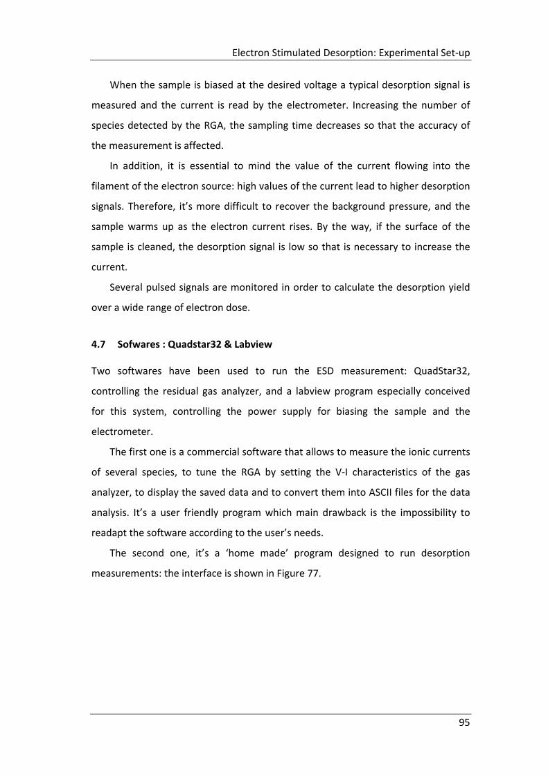
Electron Stimulated Desorption: Experimental Set‐up
95
When the sample is biased at the desired voltage a typical desorption signal is
measured and the current is read by the electrometer. Increasing the number of
species detected by the RGA, the sampling time decreases so that the accuracy of
the measurement is affected.
In addition, it is essential to mind the value of the current flowing into the
filament of the electron source: high values of the current lead to higher desorption
signals. Therefore, it’s more difficult to recover the background pressure, and the
sample warms up as the electron current rises. By the way, if the surface of the
sample is cleaned, the desorption signal is low so that is necessary to increase the
current.
Several pulsed signals are monitored in order to calculate the desorption yield
over a wide range of electron dose.
4.7 Sofwares : Quadstar32 & Labview
Two softwares have been used to run the ESD measurement: QuadStar32,
controlling the residual gas analyzer, and a labview program especially conceived
for this system, controlling the power supply for biasing the sample and the
electrometer.
The first one is a commercial software that allows to measure the ionic currents
of several species, to tune the RGA by setting the V‐I characteristics of the gas
analyzer, to display the saved data and to convert them into ASCII files for the data
analysis. It’s a user friendly program which main drawback is the impossibility to
readapt the software according to the user’s needs.
The second one, it’s a ‘home made’ program designed to run desorption
measurements: the interface is shown in Figure 77.
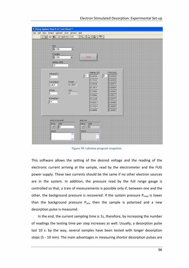
Electron Stimulated Desorption: Experimental Set‐up
96
Figure 78: Labview program snapshot.
This software allows the setting of the desired voltage and the reading of the
electronic current arriving at the sample, read by the electrometer and the FUG
power supply. These two currents should be the same if no other electron sources
are in the system. In addition, the pressure read by the full range gauge is
controlled so that, a train of measurements is possible only if, between one and the
other, the background pressure is recovered: if the system pressure Pread is lower
than the background pressure Pset, then the sample is polarized and a new
desorption pulse is measured.
In the end, the current sampling time is 1s, therefore, by increasing the number
of readings the testing time per step increases as well. Usually, a desorption pulse
last 10 s: by the way, several samples have been tested with longer desorption
steps (5 ‐ 10 min). The main advantages in measuring shorter desorption pulses are
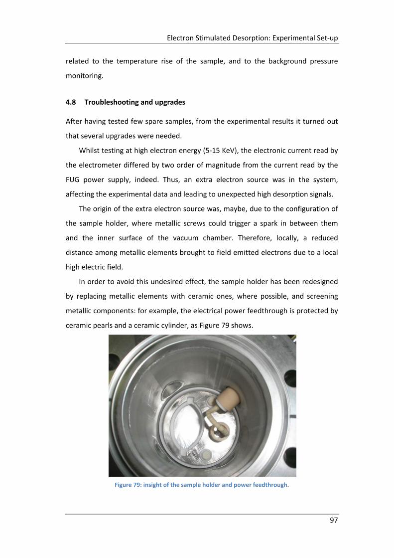
Electron Stimulated Desorption: Experimental Set‐up
97
related to the temperature rise of the sample, and to the background pressure
monitoring.
4.8 Troubleshooting and upgrades
After having tested few spare samples, from the experimental results it turned out
that several upgrades were needed.
Whilst testing at high electron energy (5‐15 KeV), the electronic current read by
the electrometer differed by two order of magnitude from the current read by the
FUG power supply, indeed. Thus, an extra electron source was in the system,
affecting the experimental data and leading to unexpected high desorption signals.
The origin of the extra electron source was, maybe, due to the configuration of
the sample holder, where metallic screws could trigger a spark in between them
and the inner surface of the vacuum chamber. Therefore, locally, a reduced
distance among metallic elements brought to field emitted electrons due to a local
high electric field.
In order to avoid this undesired effect, the sample holder has been redesigned
by replacing metallic elements with ceramic ones, where possible, and screening
metallic components: for example, the electrical power feedthrough is protected by
ceramic pearls and a ceramic cylinder, as Figure 79 shows.
Figure 79: insight of the sample holder and power feedthrough.
Electron Stimulated Desorption: Experimental Set‐up
98
In addition, a new ceramic housing for the sample holder has been done in order to
protect the metallic plate from the surrounding surfaces of the vacuum chamber.
In the end, a new rod with a magnetic manipulator has been mounted on the
upper vacuum chamber so that an easier and faster loading of the sample is
possible, without allowing any leak into the system due to the moving of the rod.
Figure 80: new rod with a magnetic manipulator.
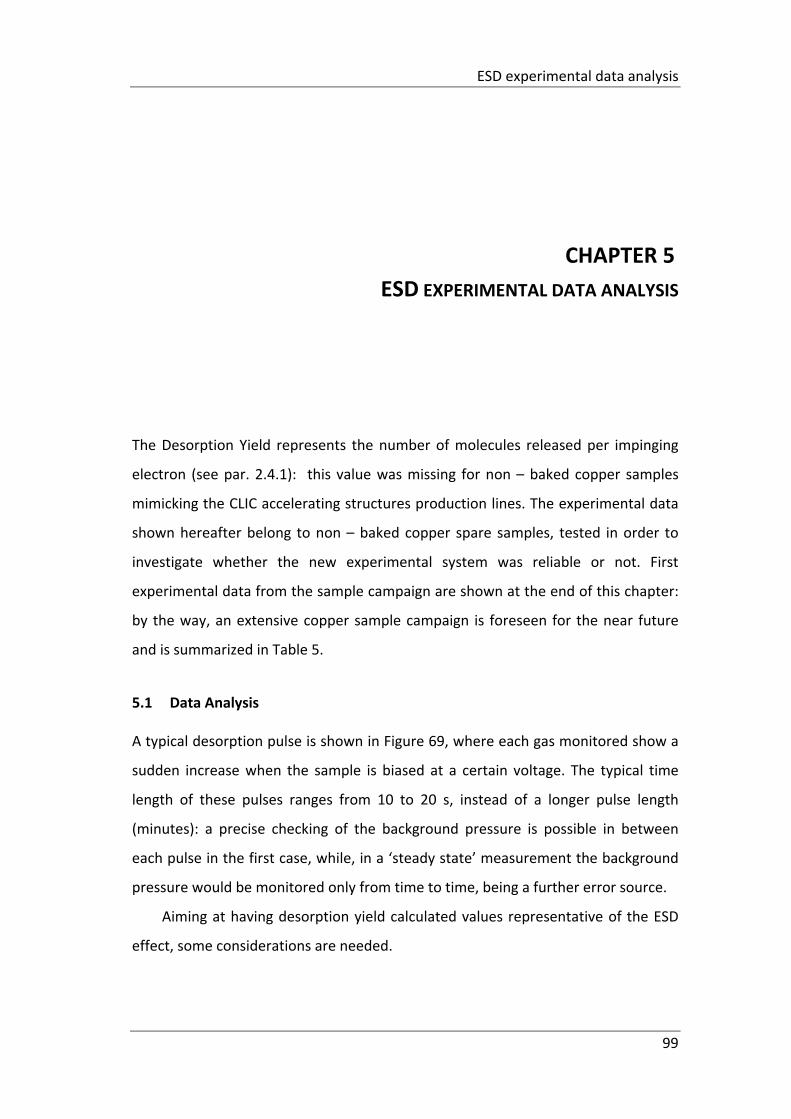
ESD experimental data analysis
99
CHAPTER 5
ESD EXPERIMENTAL DATA ANALYSIS
The Desorption Yield represents the number of molecules released per impinging
electron (see par. 2.4.1): this value was missing for non – baked copper samples
mimicking the CLIC accelerating structures production lines. The experimental data
shown hereafter belong to non – baked copper spare samples, tested in order to
investigate whether the new experimental system was reliable or not. First
experimental data from the sample campaign are shown at the end of this chapter:
by the way, an extensive copper sample campaign is foreseen for the near future
and is summarized in Table 5.
5.1 Data Analysis
A typical desorption pulse is shown in Figure 69, where each gas monitored show a
sudden increase when the sample is biased at a certain voltage. The typical time
length of these pulses ranges from 10 to 20 s, instead of a longer pulse length
(minutes): a precise checking of the background pressure is possible in between
each pulse in the first case, while, in a ‘steady state’ measurement the background
pressure would be monitored only from time to time, being a further error source.
Aiming at having desorption yield calculated values representative of the ESD
effect, some considerations are needed.
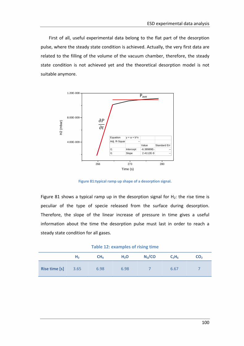
ESD experimental data analysis
100
First of all, useful experimental data belong to the flat part of the desorption
pulse, where the steady state condition is achieved. Actually, the very first data are
related to the filling of the volume of the vacuum chamber, therefore, the steady
state condition is not achieved yet and the theoretical desorption model is not
suitable anymore.
266 273 280
4.00E-009
8.00E-009
1.20E-008
H2
(m
bar)
Time (s)
Equation y = a + b*x
Adj. R-Squar --
Value Standard Err
I1 Intercept -6.38989E- --
I1 Slope 2.4112E-9 --
Figure 81:typical ramp up shape of a desorption signal.
Figure 81 shows a typical ramp up in the desorption signal for H2: the rise time is
peculiar of the type of specie released from the surface during desorption.
Therefore, the slope of the linear increase of pressure in time gives a useful
information about the time the desorption pulse must last in order to reach a
steady state condition for all gases.
Table 12: examples of rising time
H2 CH4 H2O N2/CO C2H6 CO2
Rise time [s] 3.65 6.98 6.98 7 6.67 7
Pave
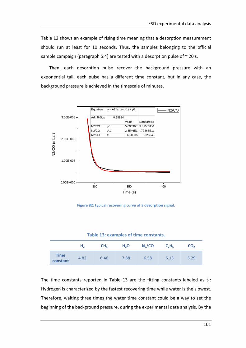
ESD experimental data analysis
101
Table 12 shows an example of rising time meaning that a desorption measurement
should run at least for 10 seconds. Thus, the samples belonging to the official
sample campaign (paragraph 5.4) are tested with a desorption pulse of ~ 20 s.
Then, each desorption pulse recover the background pressure with an
exponential tail: each pulse has a different time constant, but in any case, the
background pressure is achieved in the timescale of minutes.
300 350 4000.00E+000
1.00E-008
2.00E-008
3.00E-008
N2/
CO
(m
bar)
Time (s)
N2/COEquation y = A1*exp(-x/t1) + y0
Adj. R-Squ 0.98884
Value Standard Er
N2/CO y0 5.09696E 9.81585E-1
N2/CO A1 2.8546E1 4.79365E11
N2/CO t1 6.58335 0.25045
Figure 82: typical recovering curve of a desorption signal.
Table 13: examples of time constants.
H2 CH4 H2O N2/CO C2H6 CO2
Time constant
4.82 6.46 7.88 6.58 5.13 5.29
The time constants reported in Table 13 are the fitting constants labeled as t1:
Hydrogen is characterized by the fastest recovering time while water is the slowest.
Therefore, waiting three times the water time constant could be a way to set the
beginning of the background pressure, during the experimental data analysis. By the
ESD experimental data analysis
102
way, the value of the pressure in the system is verified by means of the dual gauge:
as long as the background pressure is not recovered, the Labview program does not
allow the setting of a new pulse.
Finally, in order to estimate the experimental errors, standard deviations have
been calculated for the pressure reached during a pulse, the background pressure
and the impinging current. The final desorption yield experimental error must take
into account all of them as Eq. 62 shows:
Δ
Eq. 63
where , and are the desorption yield standard deviation, the pressures
standard deviations and the current standard deviation, respectively. The final
formula is the following:
Eq. 64
5.2 First ESD experimental data
Hereafter are reported desorption yield experimental data as a function of the
electron dose: the trend of the desorption yield is always decreasing meaning that,
as long as the sample is bombarded with electrons, its surface is ‘cleaning’.
Therefore, lower desorption signals are expected to characterize the ESD effect at
higher electron doses.
The ESD scan for these spare samples was limited to ~ 1016 while a
complete measurement can lead to a dose equal to ~ 1020 : reaching such a
high dose is time demanding and desorption data are more likely to be affected by
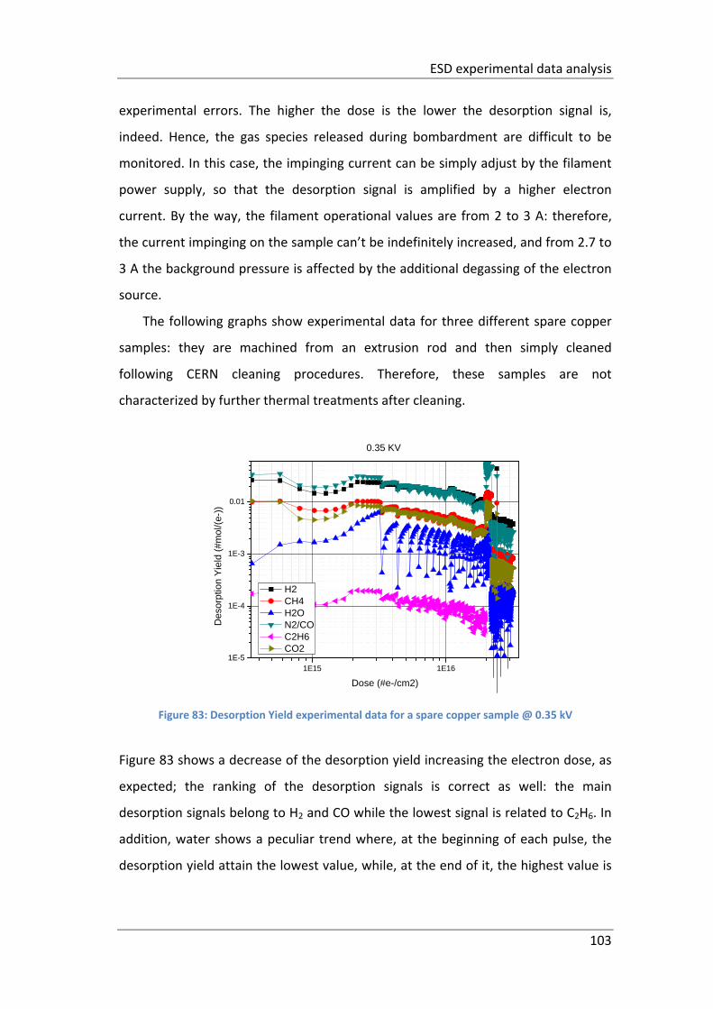
ESD experimental data analysis
103
experimental errors. The higher the dose is the lower the desorption signal is,
indeed. Hence, the gas species released during bombardment are difficult to be
monitored. In this case, the impinging current can be simply adjust by the filament
power supply, so that the desorption signal is amplified by a higher electron
current. By the way, the filament operational values are from 2 to 3 A: therefore,
the current impinging on the sample can’t be indefinitely increased, and from 2.7 to
3 A the background pressure is affected by the additional degassing of the electron
source.
The following graphs show experimental data for three different spare copper
samples: they are machined from an extrusion rod and then simply cleaned
following CERN cleaning procedures. Therefore, these samples are not
characterized by further thermal treatments after cleaning.
Figure 83: Desorption Yield experimental data for a spare copper sample @ 0.35 kV
Figure 83 shows a decrease of the desorption yield increasing the electron dose, as
expected; the ranking of the desorption signals is correct as well: the main
desorption signals belong to H2 and CO while the lowest signal is related to C2H6. In
addition, water shows a peculiar trend where, at the beginning of each pulse, the
desorption yield attain the lowest value, while, at the end of it, the highest value is
1E15 1E161E-5
1E-4
1E-3
0.01
Des
orpt
ion
Yie
ld (
#mo
l/(e-
))
Dose (#e-/cm2)
H2 CH4 H2O N2/CO C2H6 CO2
0.35 KV
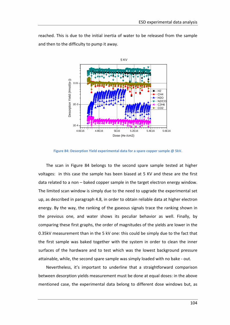
ESD experimental data analysis
104
reached. This is due to the initial inertia of water to be released from the sample
and then to the difficulty to pump it away.
Figure 84: Desorption Yield experimental data for a spare copper sample @ 5kV.
The scan in Figure 84 belongs to the second spare sample tested at higher
voltages: in this case the sample has been biased at 5 KV and these are the first
data related to a non – baked copper sample in the target electron energy window.
The limited scan window is simply due to the need to upgrade the experimental set
up, as described in paragraph 4.8, in order to obtain reliable data at higher electron
energy. By the way, the ranking of the gaseous signals trace the ranking shown in
the previous one, and water shows its peculiar behavior as well. Finally, by
comparing these first graphs, the order of magnitudes of the yields are lower in the
0.35kV measurement than in the 5 kV one: this could be simply due to the fact that
the first sample was baked together with the system in order to clean the inner
surfaces of the hardware and to test which was the lowest background pressure
attainable, while, the second spare sample was simply loaded with no bake ‐ out.
Nevertheless, it’s important to underline that a straightforward comparison
between desorption yields measurement must be done at equal doses: in the above
mentioned case, the experimental data belong to different dose windows but, as
4.6E16 4.8E16 5E16 5.2E16 5.4E16 5.6E16
1E-4
1E-3
0.01
Des
orpt
ion
Yie
ld (
#mo
l/(e-
))
Dose (#e-/cm2)
H2 CH4 H2O N2/CO C2H6 CO2
5 KV
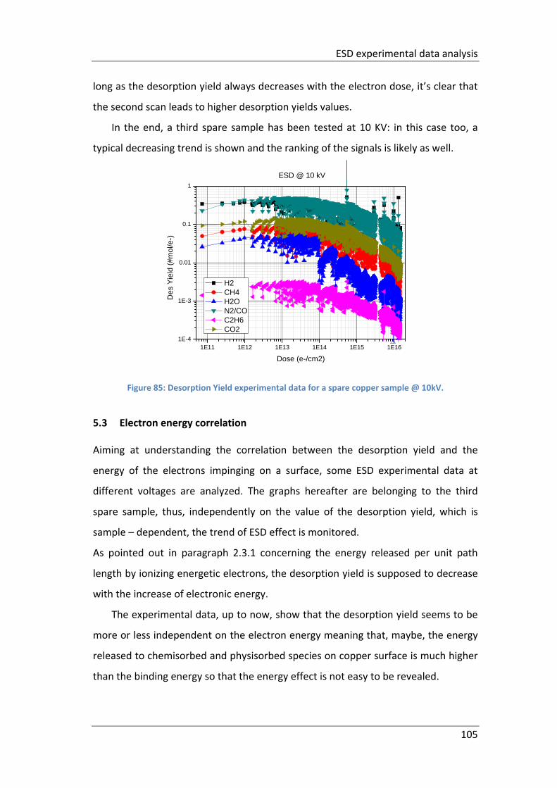
ESD experimental data analysis
105
long as the desorption yield always decreases with the electron dose, it’s clear that
the second scan leads to higher desorption yields values.
In the end, a third spare sample has been tested at 10 KV: in this case too, a
typical decreasing trend is shown and the ranking of the signals is likely as well.
1E11 1E12 1E13 1E14 1E15 1E161E-4
1E-3
0.01
0.1
1
Des
Yie
ld (
#mol
/e-)
Dose (e-/cm2)
H2 CH4 H2O N2/CO C2H6 CO2
ESD @ 10 kV
Figure 85: Desorption Yield experimental data for a spare copper sample @ 10kV.
5.3 Electron energy correlation
Aiming at understanding the correlation between the desorption yield and the
energy of the electrons impinging on a surface, some ESD experimental data at
different voltages are analyzed. The graphs hereafter are belonging to the third
spare sample, thus, independently on the value of the desorption yield, which is
sample – dependent, the trend of ESD effect is monitored.
As pointed out in paragraph 2.3.1 concerning the energy released per unit path
length by ionizing energetic electrons, the desorption yield is supposed to decrease
with the increase of electronic energy.
The experimental data, up to now, show that the desorption yield seems to be
more or less independent on the electron energy meaning that, maybe, the energy
released to chemisorbed and physisorbed species on copper surface is much higher
than the binding energy so that the energy effect is not easy to be revealed.
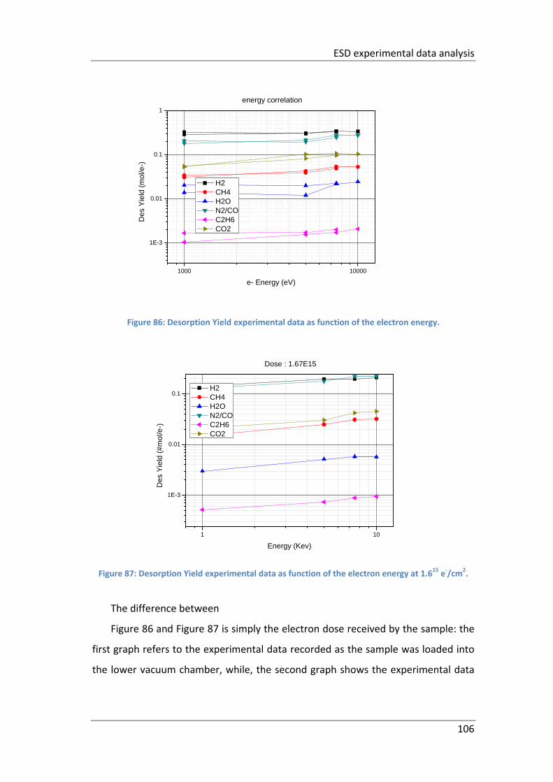
ESD experimental data analysis
106
Figure 86: Desorption Yield experimental data as function of the electron energy.
1 10
1E-3
0.01
0.1
Des
Yie
ld (
#mol
/e-)
Energy (Kev)
H2 CH4 H2O N2/CO C2H6 CO2
Dose : 1.67E15
Figure 87: Desorption Yield experimental data as function of the electron energy at 1.615 e‐/cm2.
The difference between
Figure 86 and Figure 87 is simply the electron dose received by the sample: the
first graph refers to the experimental data recorded as the sample was loaded into
the lower vacuum chamber, while, the second graph shows the experimental data
1000 10000
1E-3
0.01
0.1
1
Des
Yie
ld (
mo
l/e-)
e- Energy (eV)
H2 CH4 H2O N2/CO C2H6 CO2
energy correlation
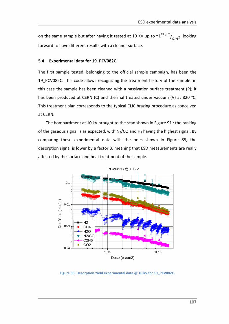
ESD experimental data analysis
107
on the same sample but after having it tested at 10 KV up to ~115 , looking
forward to have different results with a cleaner surface.
5.4 Experimental data for 19_PCV082C
The first sample tested, belonging to the official sample campaign, has been the
19_PCV082C. This code allows recognizing the treatment history of the sample: in
this case the sample has been cleaned with a passivation surface treatment (P); it
has been produced at CERN (C) and thermal treated under vacuum (V) at 820 °C.
This treatment plan corresponds to the typical CLIC brazing procedure as conceived
at CERN.
The bombardment at 10 kV brought to the scan shown in Figure 91 : the ranking
of the gaseous signal is as expected, with N2/CO and H2 having the highest signal. By
comparing these experimental data with the ones shown in Figure 85, the
desorption signal is lower by a factor 3, meaning that ESD measurements are really
affected by the surface and heat treatment of the sample.
1E15 1E161E-4
1E-3
0.01
0.1
Des
Yie
ld (
mol
/e-)
Dose (e-/cm2)
H2 CH4 H2O N2/CO C2H6 CO2
PCV082C @ 10 kV
Figure 88: Desorption Yield experimental data @ 10 kV for 19_PCV082C.
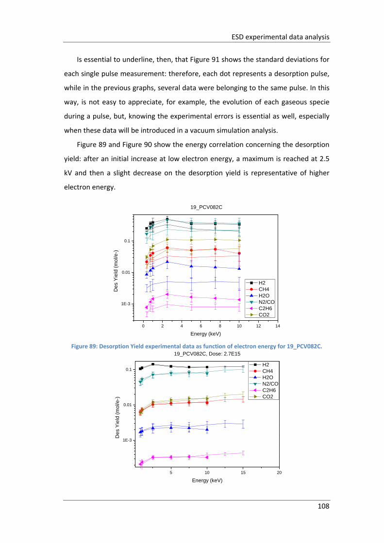
ESD experimental data analysis
108
Is essential to underline, then, that Figure 91 shows the standard deviations for
each single pulse measurement: therefore, each dot represents a desorption pulse,
while in the previous graphs, several data were belonging to the same pulse. In this
way, is not easy to appreciate, for example, the evolution of each gaseous specie
during a pulse, but, knowing the experimental errors is essential as well, especially
when these data will be introduced in a vacuum simulation analysis.
Figure 89 and Figure 90 show the energy correlation concerning the desorption
yield: after an initial increase at low electron energy, a maximum is reached at 2.5
kV and then a slight decrease on the desorption yield is representative of higher
electron energy.
Figure 89: Desorption Yield experimental data as function of electron energy for 19_PCV082C.
5 10 15 20
1E-3
0.01
0.1
Des
Yie
ld (
mo
l/e-)
Energy (keV)
H2 CH4 H2O N2/CO C2H6 CO2
19_PCV082C, Dose: 2.7E15
0 2 4 6 8 10 12 14
1E-3
0.01
0.1
Des
Yie
ld (
mo
l/e-)
Energy (keV)
H2 CH4 H2O N2/CO C2H6 CO2
19_PCV082C
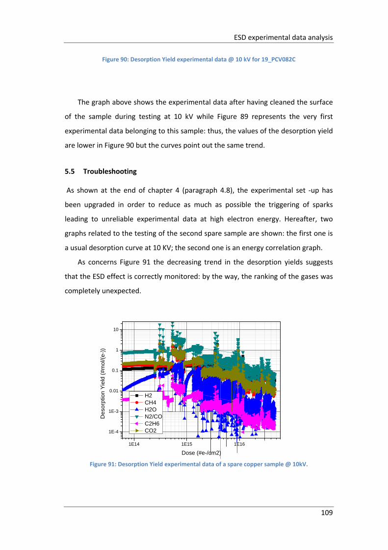
ESD experimental data analysis
109
Figure 90: Desorption Yield experimental data @ 10 kV for 19_PCV082C
The graph above shows the experimental data after having cleaned the surface
of the sample during testing at 10 kV while Figure 89 represents the very first
experimental data belonging to this sample: thus, the values of the desorption yield
are lower in Figure 90 but the curves point out the same trend.
5.5 Troubleshooting
As shown at the end of chapter 4 (paragraph 4.8), the experimental set ‐up has
been upgraded in order to reduce as much as possible the triggering of sparks
leading to unreliable experimental data at high electron energy. Hereafter, two
graphs related to the testing of the second spare sample are shown: the first one is
a usual desorption curve at 10 KV; the second one is an energy correlation graph.
As concerns Figure 91 the decreasing trend in the desorption yields suggests
that the ESD effect is correctly monitored: by the way, the ranking of the gases was
completely unexpected.
Figure 91: Desorption Yield experimental data of a spare copper sample @ 10kV.
1E14 1E15 1E16
1E-4
1E-3
0.01
0.1
1
10
De
sorp
tion
Yie
ld (
#m
ol/(
e-)
)
Dose (#e-/cm2)
H2 CH4 H2O N2/CO C2H6 CO2
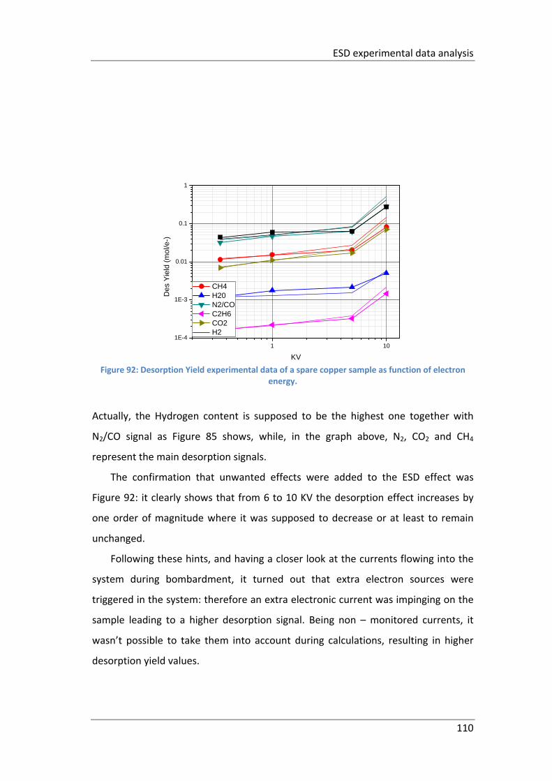
ESD experimental data analysis
110
Figure 92: Desorption Yield experimental data of a spare copper sample as function of electron energy.
Actually, the Hydrogen content is supposed to be the highest one together with
N2/CO signal as Figure 85 shows, while, in the graph above, N2, CO2 and CH4
represent the main desorption signals.
The confirmation that unwanted effects were added to the ESD effect was
Figure 92: it clearly shows that from 6 to 10 KV the desorption effect increases by
one order of magnitude where it was supposed to decrease or at least to remain
unchanged.
Following these hints, and having a closer look at the currents flowing into the
system during bombardment, it turned out that extra electron sources were
triggered in the system: therefore an extra electronic current was impinging on the
sample leading to a higher desorption signal. Being non – monitored currents, it
wasn’t possible to take them into account during calculations, resulting in higher
desorption yield values.
1 101E-4
1E-3
0.01
0.1
1
Des
Yie
ld (
mo
l/e-)
KV
CH4 H20 N2/CO C2H6 CO2 H2
ESD experimental data analysis
111
Conclusions
112
CHAPTER 6
CONCLUSIONS
The High gradient condition of CLIC accelerating structures implies facing several
problems from the static and the dynamic vacuum point of view. This Master Thesis
focused on the dynamic vacuum behavior of OFE Copper Samples produced
following the accelerating structures manufacturing flow.
A new experimental set – up has been built, and is perfectly operational, in
order to measure the desorption yield, ηi, for different species chemisorbed and
physisorbed at the surface of copper. Aiming at testing the experimental set – up
first, preliminary experimental data of spare copper samples have been analyzed
showing the need to improve the system by modifying some of its components.
Once the hardware of the system has been optimized, the first sample
belonging to the official sample campaign has been tested: the desorption yield
shows the typical decreasing trend, meaning a cleaning of the surface of the copper
sample, as expected. In addition, comparisons between the tested spare samples
and the first ‘official’ one show a dependence of the desorption yield on the surface
cleaning and heat treatment.
The correlation between the energy of the electrons impinging on the surface
of the sample and the amount of gases released has been investigated as well: the
experimental data show an increase of the desorption yield up to few keV, while
from 2.5 keV to 15 keV this latter flattens.
Conclusions
113
This experimental data will be useful as an input of dynamic vacuum simulations
which take into account the complex accelerating structure geometry. Finally, in the
near future, the whole testing campaign will be developed leading to a final choice
of the best CLIC accelerating structures production line.
BIBLIOGRAPHY
114
BIBLIOGRAPHY
1. M. Aicheler, Surface Phenomena associated with thermal cycling of copper and
their impact on the service life of particle accelerator structures, Doctoral thesis,
Bochum University, 2010
2. C. Garion: Vacuum system for the CLIC two beam modules, International
Workshop on Linear Collider 2010, Geneva
3. C. Garion: A thermal model for vacuum analysis, Technical Note, EDMS
1095288, CERN (2010)
4. J.W. Wang and G.A. Loew: Field emission and RF breakdown in copper linac
structures, Part. Acc., 30 (SLAC‐PUB‐5059):225 ‐230, Aug. 1989
5. W. Wuensch, Peak temperature rise specifications for accelerating structures: a
review and discussion, CLIC meeting presentation, CERN,(June 2010)
6. G. Riddone, Accelerating structures thermo – mechanical behavior, CLIC
meeting presentation, CERN,( June 2010)
7. M. Nonis, Cooling issues, CLIC meeting presentation, CERN,( June 2010)
8. H. Mainaud Durand, Status of the CLIC pre – alignment studies, CLIC meeting
presentation, CERN,( Apr. 2010)
BIBLIOGRAPHY
115
9. J. Osborne, CLIC civil engineering and Services Challenges, CLIC meeting
presentation, CERN,( May 2010)
10. A. Descoeudres et al.: DC breakdown conditioning and breakdown rate of
metals and metallic alloys under ultra high vacuum, Phys. Rev. ST Accel. Beams
12, 032001 (2009)
11. A. Descoeudres et al.: DC breakdown experiments with Cobalt electrodes (to be
published)
12. A. Descoeudres et al.: Investigation of the dc vacuum breakdown mechanism,
Phys. Rev.ST Accel. Beams 12, 092001 (2009)
13. H. Timko: Arcing and Plasma – Wall Interactions, University of Helsinki, (2008)
14. A. Hansen: Investigation of the Energy Dependence of breakdown properties
with a DC – spark setup, Norwegian University of Science and Technology,
(2009)
15. S. Calatroni: Progress on Investigations of Dynamic Vacuum, International
Workshop on Linear Collider 2010, Geneva
16. D. Menzel: Thirty years of MGR: How it came about, and what came of it,
Nuclear Instruments and Methods in Physics Research B 101 (1995)
17. D. Menzel, R. Gomer: Desorption from Metal Surfaces by Low‐Energy Electrons,
Journal of Chemical Physics, Vol. 41, Nb. 11 (Dec. 1964)
18. P.R. Antoniewicz: Model for electron and photon stimulated desorption,
Physical Review B, Vol. 21, Nb. 9, (May 1980)
19. W. Gortel: Beyond MGR: Wave packet squeezing, Nuclear Instruments and
Methods in Physics Research B 101 (1995)
20. P. Feulner, D. Menzel: Kinetic – Energy Distributions of Neutrals Desorbed by
Electron Impact from Adsorbates on Metal Surfaces, Physical Review Letters,
Vol. 53, Nb. 7, (Aug. 1984)
BIBLIOGRAPHY
116
21. X.Y. Zhu, J.M. White: Vibration – Mediated uv Photodesorption: Ammonia on
GaAs, Physical Review Letters, Vol. 68, Nb. 22, (June 1992)
22. W. Hubner, W. Brenig, H. Kasai: Electron Stimulated Desorption in the Anderson
model, Surface Science 226, (1990) 286 – 292
23. P. Avouris, R. E. Walkup: Fundamental mechanisms of desorption and
fragmentation induced by electronic transitions at surfaces, Annu.Rev. Phys.
Chem. (1989). 40: 173 – 206
24. J.A. Misewich, T.F. Heinz, D. M. Newns: Desorption Induced by Multiple
Electronic Transitions, Physical Review Letters, Vol. 68, Nb. 25, (June 1992)
25. K.S. Krane: Introductory Nuclear Physics, Wiley, 1988.
26. H. H. Hubbell, Jr. and R.D.Birkhoff: Calorimetric measurement of electron
stopping power of aluminum and copper between 11 and 127 keV, Physical
Review A, Vol. 26, Nb. 5, (June 1982)
27. J.C. Ashley, C.J. Tung: Electron Inelastic Mean Free Paths in Several Solids for
200 eV < E < 10 keV, Surface and Interface analysis, Vol. 4, Nb. 2 (1982)
28. J. Gomez: Temperature Dependence of Electron Induced Gas Desorption Yields
from 316 LN Stainless Steel, OFHC Cu and Al Samples, Vacuum Technical Note
94 – 16, CERN, (July 1994)
29. H. Gumus: Simple stopping power formula for low and intermediate energy
electrons, Radiation Physics and Chemistry, 72 (2005) 7 – 12
30. H. Sugiyama: Stopping power formula for intermediate energy electrons, Phys.
Med. Biol., Vol. 30, 4, 331 – 335 (1985)
31. NIST, ESTAR database : Stopping power and range tables for electrons,
www.nist.gov
32. G. Vorlaufer, Modification of Ultra – High Vacuum Surfaces Using Free Radicals,
Doctoral Thesis, CERN, (2002)
BIBLIOGRAPHY
117
33. J.M. Lafferty, Foundations of Vacuum Science and Techology, Wiley –
Interscience publications, (1998)
34. J. Crank: The Mathematics of Diffusion, Oxford Science Publications, (1975)
35. E. Fromm: Gases and Carbons in metals, Phys. Data 5 – 21, (1984)
36. B. S. Bokstein: Thermodynamics and Kinetics in materials science: a short
course, OUP Oxford, (2005).
37. D.V.Ragone: Thermodynamics of materials, Wiley, (1995)
38. D. Pitts, L. Sissom: Heat transfer, Schaum’s outlines, (1998)
39. C. Bonacina, A. Cavallini, L. Mattarolo: Trasmissione del Calore, Cleup editore,
(1989)
40. J.R.Taylor: Introduzione all’analisi delle incertezze – lo studio delle incertezze
nelle misure fisiche, Zanichelli, seconda edizione