Dipartimento di Matematica

C. Canuto, F. Cimolin

A sweating model for the internal ventilation

of a motorcycle helmet

Rapporto interno N. 6, maggio 2010

Politecnico di Torino

Corso Duca degli Abruzzi, 24-10129 Torino-Italia

A sweating model for the internal ventilation of a motorcycle

helmet

Claudio Canutoa, Flavio Cimolina,b,∗

aDipartimento di Matematica, Politecnico di Torino, Corso Duca degli Abruzzi 24, 10129 Torino, ItalybAMET S.r.l., Environment Park, Via Livorno 60, 10144 Torino, Italy

Abstract

We present a thermodynamic model for the evolution of sweat in a porous medium in contact with

a part of the human body, capable of describing the evaporation-related heat transfer phenomena.

This is suitable for the analysis and optimization of the internal ventilation of a motorcycle hel-

met, with the purpose of enhancing the comfort and ultimately the safety of the rider. The model

is based on a set of evolution equations for the three scalar unknowns temperature, absolute hu-

midity and sweat. Its mathematical properties as well as those of the numerical counterpart are

thoroughly investigated, and an efficient solution algorithm is devised. Simulations show the

onset of a free-boundary separating the wet and dry regions and highlight the zones where sweat

accumulates.

Keywords: internal fluid-dynamics, human body ventilation, sweating model, free-boundary

problem, finite elements

1. Introduction

The design of motorcycle helmets traditionally focuses on the structural performances that

they need to satisfy. Indeed its fundamental role consists in preventing injuries for the head of the

rider by absorbing and distributing the crashes occurring during accidents. Recently, industrial

manufacturers started to investigate their fluid-dynamic properties too, motivated by performance

improvement in view of races (i.e. drag reduction by mean of shape optimization) as well as

comfort-related issues such as enhanced internal ventilation systems or noise reduction [1].

Safety plays without any doubt a key role in the motorcycle helmet industrial research, whose

objective is not only to reduce injuries of the head in case of a crash (active safety), but also to

help the rider to guard against dangerous situations (passive safety). The latter issue is directly

related to the thermal comfort felt by the rider when employing this fundamental safety device:

a full-face motorcycle helmet actually generates an internal microclimate influenced by many

factors, such as sun irradiation, sweat evaporation and CO2 produced by breathing, which in

case of overly hot summer days becomes intolerable if a proper ventilation is not guaranteed.

Besides the fact that many people could be tempted not to wear the helmet at all in such cases,

∗Corresponding author

Email addresses: claudio.canuto@polito.it (Claudio Canuto), flavio.cimolin@polito.it (Flavio

Cimolin )

Preprint submitted to Computers and Fluids May 7, 2010

it has been shown that wearing a full-face helmet in uncomfortable conditions can influence the

physiological and cognitive capabilities of the rider, making him more subject to inattentions and

less reactive to threats [2].

A ventilation system is a set of channels dug across the compact protection layer of the

helmet which must be able to make some fresh external air recirculate inside it, travelling from

a series of air intakes located in the front part of the helmet towards outtakes located in the rear

one. At present helmet manufacturers suffer from a complete lack of fluid-dynamic guidelines

for the design of such channels, which are set just by experience, without sufficient confidence

of providing a proper ventilation.

This work is a first attempt of providing a numerical tool for the investigation of the internal

ventilation, achieved by means of the development of a model capable of including not only

the standard heat transfer phenomena, but also the evaporation-related ones, fundamental for

a correct analysis of the sweat removal. The application of such an approach should lead to

a better understanding of the complex phenomena of heat and sweat removal, taking place in

the (layered) porous medium between the head and the channels. Hopefully, this could be the

starting point for an investigation of different geometries and materials, in order to optimize the

global ventilation performances.

For a more detailed discussion on the model and on its properties we address the interested

reader to the Ph.D. thesis [3].

2. The sweating model

Referring to the scheme of Figure 1, consider an air flow filtrating into a porous tissue leaning

on a solid region representing a generic portion of a body. The body is supposed to release heat

and sweat from its contact interface, whose removal by conduction and convection is demanded

to the flow field. Evaporation is the fundamental phenomenon that needs to be modelled, which

is responsible of transforming sweat into water vapour, capable of being advected away form the

fabric by the airflow.

Figure 1: Sketch representation of the general problem.

A fairly realistic assumption is to keep the fluid-dynamics decoupled from the thermodynam-

ics, asserting that the presence of sweat does not affect the characteristics of the flow inside the

porous medium and that the bouyancy effects in the fluid domain can be neglected. This means

that the velocity field can be computed in a preliminary stage and then used only for what con-

cerns advection. Moreover, for simplicity, we will suppose the flow field to be defined at steady

state, thus without time dependence.

2

Since the main objective of this work is to outline and analyze the thermodynamic model

focusing on the sweat equation, we will provide just a concise description of the problem asso-

ciated with the fluid-dynamics of flow over a porous medium. The most accurate model features

a coupling of the Navier-Stokes equations in the fluid domain and the Darcy equation in the

porous one, the latter representing the simplest model for filtrating flow into a porous medium.

The coupling requires a set of three conditions on the common interface, and the solution must

be computed with rather sophisticated iterative algorithms (an extensive analysis of this coupling

can be found in [4, 5]). In order to avoid the problem of the coupling, it is possible to solve

the same equation in both the fluid and the porous domain, following the so-called “penalization

approach” [6]: the idea is to solve the Navier-Stokes equations both in the fluid and in the porous

domain, but activating in the latter one two resistance terms associated with the presence of the

porous medium. This approach is certainly less accurate than the one resulting from the cou-

pling, but is amenable to an easier implementation, especially when dealing with complex 3D

geometries. For a comparison of the two modelization approaches on a sample problem of flow

over a porous medium refer to [7].

For the sake of simplicity, we give the fluid equations for the simplest modeling approach,

namely the penalization one. The velocity and pressure field in the domain Ω = int(Ω f ∪ Ωp)

can be computed by solving the following modified set of Navier-Stokes equations:

ρ

(

∂u

∂t+ (u · ∇)u

)

− µ∆u + ∇p +

(

µ

ku +ρCF√

k|u|u

)

χΩp= 0 , (1)

together with continuity equation for an incompressible viscous flow ∇ · u = 0, where u and p

stands for the velocity field (meant as seepage velocity in the porous medium) and the pressure

respectively, ρ is the density, µ is the dynamic viscosity, k and CF are respectively the permeabil-

ity and the Forchheimer coefficient of the porous medium and χΩpis the characteristic function

of Ωp. In the following we will not deal with the fluid-dynamic problem anymore, assuming a

vector field u to be already defined on the fluid and porous domain Ω.

Let us now focus on the thermodynamic model, defining evolution equations for the follow-

ing scalar unknowns:

• T : absolute temperature (K), defined in Ω;

• h: absolute humidity, that is mass of water vapour per unit volume of air (kg/m3), defined

in Ω;

• w: sweat content in the fibers, that is mass of liquid water attached to the porous tissue per

unit volume (kg/m3), defined in Ωp.

In a few words, what intuitively happens is the following: when some sweat is released from

the body towards the porous zone, it can evaporate according to a certain rate depending on the

local values of both temperature and humidity. The evaporation process is nothing else that a

phase change, i.e. the water in liquid phase (sweat) is converted into water vapour, which can

be advected away by the flow field. The evaporation process requires energy and this causes a

temperature decrease. The coupling of the evolution equations for the three scalar unknowns lies

exactly on the reaction (evaporation) term.

The model that has been developed takes inspiration from studies related to fairly different

subjects. A model for analysing heat, water and vapour diffusion for bread baking has been

proposed in [8], later on tested on simple 3D configurations by means of finite differences and

3

finite elements in [9, 10]. In a similar fashion the problem of moisture transport in fibrous

clothing assemblies has been attacked, first from a theoretical point of view [11] and then from

the numerical one using finite volumes [12]. Furthermore, a slightly less comprehensive model

has been developed in order to study the cooling of grain bins [13], implemented numerically in

[14].

Starting from the simplest equation, the evolution of the temperature in Ω is given by

C∂T

∂t+C f u · ∇T = ∇ · (λ∇T ) − les(h,T,w), (2)

where C is the equivalent volumetric heat capacity, C f the volumetric heat capacity of the fluid, λ

the equivalent thermal conductivity coefficient, le is the latent heat of vaporization and s(h,T,w)

is the evaporation rate. Since we are dealing with two different domains, the equivalent volumet-

ric heat capacity is defined as

C =

C f in Ω f ,

nC f + (1 − n)Cp in Ωp,(3)

n being the porosity of the porous medium and Cp being the volumetric heat capacity of the

solid component of the medium [15, 16]. A similar definition holds for the equivalent thermal

conductivity λ, which can be computed in the two domains according to the values of λ f and λp

associated respectively to the fluid and to the solid constituent of the porous medium.

For what concerns the evolution of the absolute humidity, we consider it as diffused in the

air, thus setting for its evolution the following advection-diffusion-reaction equation that holds

in Ω:∂h

∂t+ u · ∇h = Dh∆h + s(h,T,w), (4)

where the constant Dh is the diffusivity of water vapour in air [17].

Finally, for the evolution of the sweat content in the fibers of the porous medium, we consider

in Ωp

∂w

∂t= ∇ · (Dw∇w) − s(h,T,w), (5)

where Dw is a diffusivity coefficient of the sweat in the porous tissue.

The system of three advection-diffusion-reaction equations for T , h and w is coupled by

means of the non-linear reaction term associated with evaporation, which can be expressed as

s(h,T,w) = σ(h,T ) χw+ , (6)

where the dependence on sweat is given by the second factor χw+ , that is the indicator function

for the wet domain

χw+ (x, t) =

1 if w(x, t) > 0,

0 if w(x, t) ≤ 0.(7)

This term simply states that evaporation takes place only where there is water: without sweat

there is certainly no evaporation. This is quite a neat modeling assumption, since what really

happens physically is somehow a little more gradual and smooth. However, this approximation

is coherent with the mathematical model, as we will highlight in the following sections, and it

agrees with physical intuition.

4

The actual dependence of the evaporation rate from the temperature and humidity can be

obtained by a three dimensional extension of the Hertz-Knudsen formula [18]

σ(h,T ) = E

√

Mv

2πRT

(

psat(T ) − pv(h,T ))

, (8)

where E is the evaporation coefficient, Mv is the molecular weight of water vaporus, R is the

ideal gas constant, whereas pv and psat are the vapour pressure and saturation vapour pressure

respectively. They are given by the following psychrometric formulas [19]: the vapour pressure

can be expressed by means of the ideal gas law as

pv(h,T ) =hRT

Mv

, (9)

whereas the saturation vapour pressure, i.e. the partial pressure of the vapour when in a close

system the equilibrium between its liquid phase is obtained, can be approximated by the experi-

mental formula of Magnus-Tetens by

psat(T ) = 611.2 exp

(

17.62T − 273.15

T − 30.03

)

, (10)

which is accurate in the range of temperatures between 228 K and 333 K.

Note that the saturation vapour pressure can be viewed as linked to the maximum content

of water vapour per unit volume that can exist in gaseous phase at a certain temperature. This

leads to the well-known definition of relative humidity (usually expressed as a percentage) as

RH = pv/psat.

Of course the model described by Equations (2), (4) and (5) need to be associated with a

suitable set of initial and boundary conditions for the unknowns T , h and w. Keeping it in the

most general form, we can consider for the temperature

T = T on γTD, λ

∂T

∂n= Q on γT

N , (11)

having split the boundary of Ω into its Dirichlet and Neumann parts as ∂Ω = γTD∪ γT

N, with

γTD∩ γT

N= ∅.

Similarly, for the boundary conditions related to the absolute humidity we will have

h = h on γhD, Dh

∂h

∂n= R on γh

N , (12)

with ∂Ω = γhD∪ γh

N, γh

D∩ γh

N= ∅, and for the boundary conditions associated with sweat we

consider

w = w on γwD, Dw

∂w

∂n= S on γw

N , (13)

with ∂Ωp = γwD∪ γw

N, γw

D∩ γw

N= ∅. The boundary γw

Nis fundamental since we assume S ≥ 0

therein, and in particular S > 0 on some non-empty part of γwN

; in other words we assume that

some sweat is entering the domain.

Note that a homogeneus Neumann condition on the temperature or on the absolute humidity

can be used in order to model two different physical conditions, namely an adiabatic condition

on a wall at which u ·n = 0 or an outlet condition with null diffusive flux on a boundary portion at

5

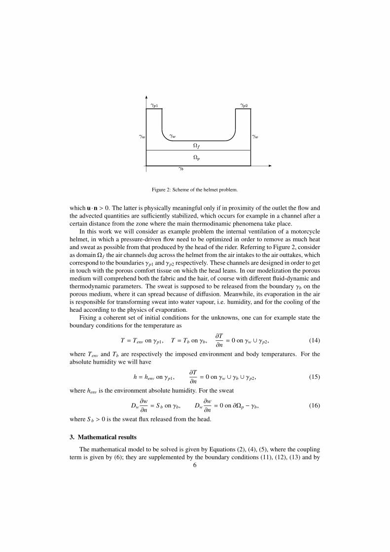
Figure 2: Scheme of the helmet problem.

which u ·n > 0. The latter is physically meaningful only if in proximity of the outlet the flow and

the advected quantities are sufficiently stabilized, which occurs for example in a channel after a

certain distance from the zone where the main thermodinamic phenomena take place.

In this work we will consider as example problem the internal ventilation of a motorcycle

helmet, in which a pressure-driven flow need to be optimized in order to remove as much heat

and sweat as possible from that produced by the head of the rider. Referring to Figure 2, consider

as domainΩ f the air channels dug across the helmet from the air intakes to the air outtakes, which

correspond to the boundaries γp1 and γp2 respectively. These channels are designed in order to get

in touch with the porous comfort tissue on which the head leans. In our modelization the porous

medium will comprehend both the fabric and the hair, of course with different fluid-dynamic and

thermodynamic parameters. The sweat is supposed to be released from the boundary γb on the

porous medium, where it can spread because of diffusion. Meanwhile, its evaporation in the air

is responsible for transforming sweat into water vapour, i.e. humidity, and for the cooling of the

head according to the physics of evaporation.

Fixing a coherent set of initial conditions for the unknowns, one can for example state the

boundary conditions for the temperature as

T = Tenv on γp1, T = Tb on γb,∂T

∂n= 0 on γw ∪ γp2, (14)

where Tenv and Tb are respectively the imposed environment and body temperatures. For the

absolute humidity we will have

h = henv on γp1,∂T

∂n= 0 on γw ∪ γb ∪ γp2, (15)

where henv is the environment absolute humidity. For the sweat

Dw

∂w

∂n= S b on γb, Dw

∂w

∂n= 0 on ∂Ωp − γb, (16)

where S b > 0 is the sweat flux released from the head.

3. Mathematical results

The mathematical model to be solved is given by Equations (2), (4), (5), where the coupling

term is given by (6); they are supplemented by the boundary conditions (11), (12), (13) and by

6

suitable initial conditions.

In view of the application of a fixed-point argument, we discuss the solvability of each scalar

advection-diffusion-reaction equation, given the other two unknowns. For Equations (2) and

(4), existence and uniqueness follow from classical results (see, e.g. [20]), since the non-linear

function σ(h,T ) is bounded and smooth in the range of validity of the model.

Concerning Equation (5), it is not restrictive to assume Dw = k constant, and w = 0 on

ΓD = γwD

. Setting a(x, t) = σ(

h((x, t),T (x, t))

, we thus consider the problem

∂w

∂t− k∆w + aχw+ = 0 in Ωp, t > 0,

w = 0 on ΓD, k∂w

∂n= S on ΓN = γ

wN ,

(17)

plus the initial condition w(x, 0) = w0(x), x ∈ Ωp. The corresponding weak formulation reads:

find w(t) ∈ V =

v ∈ H1(Ωp) : v = 0 on ΓD

such that

d

dt

∫

Ωp

w(t)v + k

∫

Ωp

∇w(t) · ∇v +

∫

Ωp

aχw(t)+v =

=

∫

ΓN

S v ∀v ∈ V, t > 0. (18)

Let us assume that a ≥ 0 in Ωp. Then we note that for any w1,w2 ∈ V one has

∫

Ωp

(

aχw+1− aχw+

2

)

(w1 − w2) =

=

∫

w1>0a(w1 − w2) −

∫

w2>0a(w1 − w2) =

=

∫

w1>0,w2≤0a(w1 − w2) +

∫

w2>0,w1≤0a(w2 − w1) ≥ 0. (19)

Thus, the operator A : V → V ′ defined by

⟨

A(w), v⟩

= k

∫

Ωp

∇w · ∇v +

∫

Ωp

aχw+v −∫

ΓN

S v, (20)

satisfies⟨

A(w1) − A(w2),w1 − w2

⟩ ≥ k

∫

Ωp

|∇(w1 − w2)|2 > 0 if w1 , w2, (21)

i.e. it is a maximal-monotone coercive operator in V . Hence, existence and uniqueness of the

solution of (17) follow from abstract results on those operators (see, e.g., [21, 22]).

A complementary perspective is obtained by introducing the convex functional j(w) =∫

Ωpaw+

on V . It is easily seen that for any w ∈ V one has

limδ→0

j(w + δv) − j(w)

δ=

∫

w=0av+ +

∫

w>0av ∀v ∈ V. (22)

Thus, if measw = 0 = 0, then j is Frechet differentiable at w and j′(w) = aχw+ , i.e. ∂ j(w) =

aχw+ . On the other hand, if measw = 0 > 0, then for any δ > 0

j(w + δv) − j(w)

δ≥

∫

w=0av+ +

∫

w>0av ≥

∫

Ωp

agv ∀v ∈ V, (23)

7

where g : Ωp → [0, 1] is any function satisfying g(x) = 0 on w < 0 and g(x) = 1 on w > 0.This means that the subdifferential ∂ j(w) (see, e.g. [23]) is the collection of the functions ag; in

particular, aχw+ ∈ ∂ j(w).

Introducing the strictly convex functional on V

J(w) =k

2

∫

Ωp

|∇w|2 + j(w) −∫

ΓN

S w, (24)

one has

∂J(w) = B(w) + ∂ j(w), (25)

where⟨

B(w), v⟩

= k

∫

Ωp

∇w · ∇v −∫

ΓN

S v ∀v ∈ V. (26)

Then, (18) can be written as

∂w(t)

∂t+ ∂J

(

w(t)) 3 0 t > 0, (27)

showing that (17) is a gradient flow equation. An alternative approach, based on the theory of

variational inequalities, could be adopted as well.

The situation in which a < 0 in some parts of the domain, corresponding to a localized

condensation of water vapour is in principle admissible, although of limited interest in this appli-

cation; mathematically, its treatment is non-trivial (see, e.g. [24]). From now on, we will assume

that a ≥ 0 throughout Ωp.

3.1. Non-negativity of the solution w

Using standard variational arguments, we can prove a maximum principle for w: if w0 ≥ 0 in

Ωp, w ≥ 0 on γwD

and S ≥ 0 on γwN

, then w(t) ≥ 0 in Ωp for all t ≥ 0. To this end (assuming as

before w = 0), we express w as w = w+ − w−, where w− = max(−w, 0). Choosing v = w− as test

function in (18) and using the properties

∫

Ωp

w+w− =

∫

Ωp

∇w+ · ∇w− = 0,

∫

w>0aw− = 0, (28)

we obtaind

dt

∫

Ωp

|w−|2 = −k

∫

Ωp

|∇w−|2 −∫

γwN

S w− ≤ 0; (29)

since w−(0) = 0 by assumption, we conclude that w−(t) = 0 for all t > 0, i.e. the thesis.

Note that the crucial property∫

w>0 aw− = 0 holds irrespectively of the sign of a; in other

words, even if a > 0 and the term aχw+ in (17) has the effect of lowering w wherever it is

positive, the solution is never pushed below zero. This is coherent with the physical meaning of

the variable w, which represents the concentration of sweat.

The domainΩp is thus partitioned into two regions depending on time: the wet region, where

w(x, t) > 0, and the dry region, where w(x, t) = 0. The interface between the two regions is

investigated below.

8

3.2. Considerations on the movement of the interface

If in Equation (17) we remove the time derivative term in order to look for a steady-state

solution for the 1D sweat equation, we obtain the following two-point boundary-value problem:

−kw′′ = −aχw+ in (0, 1),

w(0) = 0 , kw′(1) = b,(30)

where for convenience we set b = S .

The solution is known to be non-negative throughout [0, 1]. Whether a free-boundary, sepa-

rating the regions w = 0 and w > 0, appear depends on the relative size of a and b. Indeed, it is

easy to check that

• if b ≥ a one has (see Figure 3.i)

w(x) =b − a

kx +

a

2kx2; (31)

• if b < a, setting α = 1 − b/a, one has (see Figure 3.ii)

w(x) =

(a − b)2

2ak+

b − a

kx +

a

2kx2 x ≥ α,

0 x < α.

(32)

0.2 0.4 0.6 0.8 1.0 x

1

2

3

4

5

6

7

w

0.2 0.4 0.6 0.8 1.0 x

0.5

1.0

1.5

w

(i) (ii)

Figure 3: Different types of solutions of Problem (30).

Note that in the second case the solution vanishes in an entire subdomain (0, α), called the

null core of the solution [25, 26]. This feature is in agreement with the physical interpretation

of the model: the sweat provided from the right boundary diffuses inside the domain and the

movement of the interface between the null core and the zone where sweat is present depends

on the balance between what is provided as Neumann condition (b) and what is removed by

evaporation (a).

For the unsteady problem

∂w

∂t− k∂2w

∂x2= −aχw+ in (0, 1),

w(0, t) = 0 , k∂w

∂x(1, t) = b , w(x, 0) = 0,

(33)

9

it is possible to perform a qualitative study of the movement of the interface α(t) near the initial

condition by approximating the time derivative with its first order increment

∂w

∂t(x,∆t) ≈ 1

∆t

(

w(x,∆t) − w(x, 0))

=1

∆tw(x,∆t). (34)

The corresponding equation

1

∆tw − kw′′ = −aχw+ in

(

α(∆t), 1)

, (35)

together with its boundary conditions

w(

α(∆t))

= 0 , kw′(1) = b , w′(

α(∆t))

= 0, (36)

can be solved analytically for the first time increment, leading to the following asymptotic be-

haviour in proximity of t = 0:

α(∆t) ≈ 1 − 1

2

√k∆t

∣

∣

∣

∣

ln(√

k∆t)∣

∣

∣

∣

. (37)

As an example, the movement of the interface α(t) for Problem (33) with k = 1, a = 8, b = 4,

which leads to the steady-state position α = 1/2, is shown in Figure 4, obtained numerically as

described later on.

0.0 0.1 0.2 0.3 0.4t

0.6

0.7

0.8

0.9

1.0ΑHtL

Figure 4: Position of the interface.

4. Time discretization

4.1. The sweat equation

Let us first discuss Equation (17). While the diffusive term is invariably treated implicitly,

the non-linear term can be discretized in a fully explicit or in a semi-implicit way.

Considering the latter case, using e.g. the implicit Euler scheme and setting wn ≈ w(tn) with

tn = n∆t, n = 0, 1, . . . , we have

1

∆t

(

wn+1 − wn) − k∆wn+1 + anχ(wn+1)+ = 0 in Ωp, n ≥ 0. (38)

10

For each n, this steady problem admits existence and uniqueness, since it is of the form An(wn+1) =

0, where An : V → V ′, defined by

⟨

An(w), v⟩

=1

∆t

∫

Ωp

(

w − wn)v +⟨

B(w), v⟩

+

∫

Ωp

anχw+v ∀v ∈ V, (39)

is again a maximal-monotone coercive operator in V .

Introducing the functionals jn(w) =∫

Ωpanw+ and

En(w) =1

2∆t

∫

Ωp

(

w − wn)2+

k

2

∫

Ωp

|∇w|2 + jn(w) −∫

ΓN

S w, (40)

one has

∂En(w) =1

∆t

(

w − wn) + B(w) + ∂ jn(w); (41)

since An(

wn+1)

= 0, we have

0 ∈ ∂En(wn+1), (42)

which proves that wn+1 is the (unique) minimum point of the strictly convex functional En(w). In

other words, we have

En(wn+1) = minv∈VEn(v). (43)

Using the same arguments as above, it is easily seen that the maximum principle holds again,

i.e. wn ≥ 0 for all n under the same positivity hypotheses of the time-dependent problem.

For the a priori and a posteriori error analysis of this time discretization scheme we refer to

[27].

The fully explicit version of the non-linear term is given by anχ(wn)+ . In this case, at each

time step one has to solve a linear Helmholtz-type equation, a cheaper task than solving the

minimization problem (43); however, the maximum principle is no longer valid and actually, the

solution may become negative in proximity of the interface.

To better clarify the above considerations it is useful to focus on the 1D example problem

(33), monitoring the value of the total mass of sweat M =∫

Ωpw(t) as a function of time. For

suitable values of the model parameters (e.g. a = 8, b = 4, k = 1) the exact solution converges

towards the steady-state solution given by (32).

The following three different approaches have been tested on a 1D grid made of 20 elements

on the [0, 1] interval, for the unsteady simulation with ∆t = 0.02 and final time T f = 2.0 (the

related values ofM are plotted in Figure 5):

• Explicit scheme (blue line).

• Pseudo-implicit scheme with under-relaxation (red line).

• Minimization scheme (black line).

Using the fully explicit treatment of the non-linear term, the integral monitor does not con-

verge, starting to oscillate in time near the exact solution; the oscillation width scales with ∆t.

Indeed, if the evaporation term is not computed implicitly, at each timestep the sweat content in

proximity of the interface is once too much and once too less with respect to its theoretical steady

value. Thus this approach is cheap but not accurate, unless a really small timestep is choosen.

11

0.0 0.5 1.0 1.5 2.0t0.00

0.05

0.10

0.15

0.20Ù w

Figure 5: Total mass of sweatM computed with the three different advancing schemes, using the same timestep ∆t.

On the other hand, using the minimization approach described above, the curve ofM grows

smooth towards the steady-state value, giving the most accurate approximation of the exact so-

lution of the sweat equation. This approach is stable for whatever timestep size (even computing

directly the steady-state solution, i.e. with ∆t → +∞), but fairly expensive in terms of computa-

tional cost, since a complete minimization needs to be performed at each timestep.

Finally, the pseudo-implicit scheme is a rather less elegant approach which however can be

shown to be really efficient for the computation of the steady-state solution. Equation (45) is

substituted by the sequence of equations for p = 1, 2, . . . , P

wn+1,p+1 − wn

∆t= ∇ · (Dw∇wn+1,p+1) − σnχ(wn+1,p)+ , (44)

with wn+1,1 = wn. At each timestep, P “inner iterations” are completed, at the end setting wn+1 =

wn+1,P. The increment wn+1 − wn is corrected by means of an under-relaxation factor β which

is reduced as converence towards the steady state is observed, i.e. proportionally to (‖wn+1‖ −‖wn‖)/‖wn+1‖.

If the under-relaxation parameter and its evolution are suitably calibrated, this pseudo-implicit

scheme converges fastly towards the same stead state solution obtained by minimization will

less computational efforts, as can be seen in Figure 5. Moreover, this approach is easily imple-

mentable on a commercial CFD code for the analysis of concrete 3D models, which is an issue

that needs to be taken into account for the application.

4.2. The complete system

At last, we consider the time discretization of the coupled system (2), (4), (5). We adopt

an implicit Euler scheme for the linear (diffusion and advection) terms in each equation, the

semi-implicit Euler scheme discussed above for the non-linear term in the sweat equation, and a

fully explicit Euler scheme for the temperature and absolute humidity equations. In such a way,

the three equations are decoupled at each timestep, and the more expensive implicit treatment is

confined to the sweat equation only, which is the most critical one in the model.

The resulting algorithm reads as follows:

12

1. Compute the regular part of the evaporation term σn = σ(hn,T n).

2. Solve the sweat equation

wn+1 − wn

∆t= ∇ · (Dw∇wn+1) − σnχ(wn+1)+ . (45)

3. Solve the equation for the temperature

CT n+1 − T n

∆t+C f u · ∇T n+1 = ∇ · (λ∇T n+1) − leσ

nχ(wn+1)+ . (46)

4. Solve the equation for the absolute humidity

hn+1 − hn

∆t+ u · ∇hn+1 = Dh∆hn+1 + σnχ(wn+1)+ . (47)

Results of the complete coupled system for a sample helmet ventilation problem will be

shown in Section 6.

5. Space discretization

The spatial discretization of Equations (45), (46) and (47) is accomplished by the Galerkin

method using finite dimensional subspaces made of continuous, piecewise linear finite elements

on a triangular mesh Th in each of the domains Ω f and Ωp. The non-linear term σn is approxi-

mated by a piecewise constant function σnh

on the mesh. Figure 6 shows a structured triangular

mesh on a square, together with an example of steady-state solution for the sole sweat equation,

in which sweat is provided from the bottom and right-hand sides, while on the others an adiabatic

condition is set.

Figure 6: Steady-state solution for the sweat equation in a 2D domain (logarithmic scale).

We focus again on the sweat equation, in the form (38). The Galerkin scheme amounts to

finding wn+1h∈ Vh ⊂ V satisfying

⟨

Anh(wn+1

h , vh

⟩

=1

∆t

∫

Ωp

(

wn+1h − wn

h

)

vh + k

∫

Ωp

∇(wn+1h

) · ∇vh+

+

∫

Ωp

anhχ(wn+1

h)+vh −

∫

ΓN

S vh = 0 ∀vh ∈ Vh, (48)

13

where Vh =

v ∈ V : v|T ∈ P1(T ),∀T ∈ Th,T ⊂ Ωp

. Existence and uniqueness of the solution

follow from the maximal-monotonicity and coerciveness of Anh

in Vh. Introducing the functional

jnh(w) =

∫

Ωpan

hw+, and defining En

h(w) in the obvious way as in (40), we obtain

Enh(wn+1

h ) = minvh∈Vh

Enh(vh), (49)

i.e., wn+1h

can be computed by solving a minimization problem. To be precise, at each timestep

the optimization task is performed by the gradient method with quadratic linesearch.

The non-negativity of the discrete solution can be easily established under the assumption

that all the triangles in Th are acute-angled and that numerical integration (mass lumping) is

applied to the zeroth-order term 1∆t

∫

Ωp

(

wn+1h− wn

h

)

vh and to the non-linear term∫

Ωpan

hχ(wn+1

h)+vh.

In this case, the algebraic equation corresponding to (48) at the node x j has the form

∑

l

(

1

∆tm jδ jl + ks jl

)

wn+1l + an

jm j

(

wn+1j

)+=

=1

∆tm jw

nj + δ jΓN

∑

l′

m jl′S l′ (50)

where s jl are the entries of the stiffness matrix, m j are the entries of the diagonal lumped mass

matrix, δ jΓN= 1 if x j ∈ ΓN and 0 otherwise, and m jl′ are the entries of the 1D mass matrix of

ΓN . If we assume that there exists j such that wn+1j= min wn+1

l< 0, then

(

wn+1j

)+= 0. Using the

properties s j j > 0, s jl < 0 if j , l,∑

l s jl = 0 and the assumption wnh≥ 0, S ≥ 0, we have

wn+1j ≥

k∑

l, j |s jl|wn+1l

1∆t

m j + ks j j

≥ks j j

1∆t

m j + ks j j

wn+1j > wn+1

j , (51)

a contradiction.

A more accurate discretization is obtained by applying the mass lumping to the zeroth-order

term only; even in this case, non-negativity is observed. In the functional Enh

to be minimized,

now the non-linear term jnh(w) is integrated exactly, without interpolation at the nodes. For

example in 1D with continuous piecewise linear elements it can be obtained as

∫

Ωp

anhw+ =

∑

T∈Th

anhT

∫

T

w+ =∑

T∈Th

anhT

g∗(w|T ), (52)

where g∗(w|T ) = g∗(

w(xa),w(xb))

is given by

12(b − a)

(

w(xa) + w(xb))

if w(xa) ≥ 0 and w(xb) ≥ 0,12(b − a)

w(xa)2

w(xb)−w(xa)if w(xa) < 0 and w(xb) ≥ 0,

0 if w(xa) < 0 and w(xb) < 0,

(53)

the second case being clarified by Figure 7.

As a final remark, we note that when applying the explicit or pseudo-implicit time discretiza-

tion schemes described in Section 4.1, the characteristic function χw+ should be replaced by its

“discrete version” χw+ defined by means of a threshold value wth > 0 below which it is assumed to

be zero (for example wth = 10−6), in order to filtrate the roundoff errors associated with machine

precision.

14

Figure 7: Integral of the positive part in 1D.

6. Results

In view of a concrete application of the model to a real 3D configuration of the channels of a

helmet, we start by investigating the behaviour of the model on an “approximated” 2D geometry

like the one of Figure 2, the horizontal length and width of the channel being 200 mm and 4 mm

respectively. As a modeling assumption, we subdivide the porous domain Ωp in two different

portions characterized by different physical parameters: a 3 mm layer of comfort tissue below

which there is a 4 mm layer of “hair and air”. Indeed, the definition of sweat content on the fibers

can be meant to be applied to the hair as well as to the actual fibers of the foam.

The airflow in the channel and porous media (namely the velocity field u, shown in Figure

9), which here we assume to be a datum of the problem, has been numerically computed in

a preliminary stage solving the penalized Navier-Stokes equations (1) with a pressure gap of

2.0 Pa between the inlet γp1 and the outlet γp2.

Starting from a coherent initial condition for h and T , and with w = 0 at t = 0, we analyze now

the results obtained at steady state for the following problem variables (referring to Equations

(14), (15), (16)):

• environment temperature Tenv = 305 K, head temperature Tb = 310 K;

• environment absolute humidity henv = 2.0 · 10−2 kg/m3, corresponding to a relative humid-

ity RH = 60% at the environment temperature Tenv;

• sweat flux from the head S b = 3.5 · 10−5 kg m−2 s−1.

The parameters of the model are collected in Table 1.

The steady-state solution has been computed by means of the finite element code freeFEM++

[28] on an unstructured grid of approximately 56, 000 triangles generated automatically inside

the program. The sweat distribution in the porous domain is shown in Figure 10, from which

the interface between the wet and the dry zone is clearly identifiable. As expected, the highest

concentrations of sweat are located at the right-end side of the domain, where the evaporation

rate decreases as the air gets more and more saturated by water vapour.

The values of w along vertical sections at different stations of the porous media are reported

in Figure 8, from which the essentially parabolic behaviour is clearly evinced as well as the

different properties of the two distinct porous layers.

Besides sweat, it is also interesting to observe the distribution of the two other scalar un-

knowns, namely absolute humidity (Figure 12) and temperature (Figure 11), since the interac-

tion between all of them helps understanding what physically happens inside the channel. While

15

Parameter Value Unit

C f 1.2 · 103 J m−3 K−1

Cp, f abric 1.7 · 106 J m−3 K−1

Cp,hair 1.7 · 105 J m−3 K−1

λ f 0.026 W m−1 K−1

λp, f abric 0.16 W m−1 K−1

λp,hair 0.37 W m−1 K−1

n f abric 0.9 -

nhair 0.99 -

Dh 2.56 · 10−5 m2/s

Dw, f abric 10−8 m2/s

Dw,hair 10−7 m2/s

E 5.0 · 10−3 m−1

R 8.314 J K−1 mol−1

Mv 1.802 kg/mol

le 2.428 · 106 J/kg

Table 1: Physical parameters employed in the simulation.

0 1 2 3 4 5 6 7y0.0

0.5

1.0

1.5

2.0

2.5w

Figure 8: Values of w on different vertical sections of the porous domain at x = 50 (blue), x = 100 (red), x = 150 (green)

and x = 190 (magenta).

16

the absolute humidity plot simply highlights the advection of water vapour, i.e. the evaporated

sweat, the temperature field shows a somehow unpredictable behaviour, in which the lowest tem-

perature, located in a quite advanced position of the porous tissue, turns out to be even below the

environment temperature imposed in the inlet.

Besides these qualitative results, it is possible to consider some important quantitative mon-

itors for the “de-sweating performance” of the channel, such as the total mass of sweat in the

porous domainM and the heat flux Q from the “head boundary” γb,

M =∫

Ωp

w ≈ 4.862 · 10−4 kg, Q =∫

γb

λp

∂T

∂n≈ −16.60 W. (54)

They could be employed to compare different geometries as well as different materials in order

to optimize the channel ventilation performances.

Figure 9: Vector plot of the velocity field u, meant as seepage velocity in the porous domain.

Figure 10: Contour plot of the sweat w in the porous domain (logarithmic scale).

7. Summary

A thermodynamic model for the analysis of the internal ventilation for a motorcycle helmet,

capable of describing both the heat transfer and the sweating-related phenomena, has been out-

lined. It is based on the coupled evolution of the three scalar unknowns temperature, absolute

17

Figure 11: Contour plot of the temperature T .

Figure 12: Contour plot of the absolute humidity h .

18

humidity and sweat (defined only in the porous domain as a density attached to the fibers), linked

by means of the evaporation term.

The mathematical well-posedness of the problem has been assessed and a proof of non-

negativity of the sweat has been given. Some properties on the free boundary between the wet

and the dry zone have been discussed.

Thereafter, the numerical resolution has been detailed, starting from the time-advancing

scheme and concluding with the finite element spatial discretization. The most accurate scheme

for the numerical solution of the sweat equation turned out to be associated to the minimization

of a functional, that need to be carried out at each timestep.

Finally, the whole thermodynamic model has been numerically solved for a sample 2D prob-

lem and the results have been discussed and interpreted.

8. Acknowledgements

The authors wish to thank R. Nochetto, G. Savare and P. Tilli for fuitful discussions.

References

[1] P. Pinnoji, P. Mahajan, Impact analysis of helmets for improved ventilation with deformable head model, in: IR-

COBI Conference, Madrid, Spain., 159–170, 2006.

[2] C. Bogerd, Physiological and cognitive effects of wearing a full-face motorcycle helmet, Ph.D. thesis, ETH Zurich,

Zurich, Switzerland, 2009.

[3] F. Cimolin, Analysis of the internal ventilation for a motorcycle helmet, Ph.D. thesis, Politecnico di Torino, Italy,

2010.

[4] M. Discacciati, Domain Decomposition Methods for the Coupling of Surface and Groundwater Flows, Ph.D. thesis,

Ecole Polytechnique Federale de Lausanne, Switzerland, 2004.

[5] M. Discacciati, A. Quarteroni, Navier-Stokes/Darcy coupling: modeling, analysis, and numerical approximation,

Rev. Mat. Complut. 22 (2) (2009) 315–426.

[6] C. Bruneau, I. Mortazavi, Numerical modelling and passive flow control using porous media, Computers & Fluids

37 (2008) 488–498.

[7] F. Cimolin, M. Discacciati, Navier-Stokes/Forchheimer models for filtration through porous media, Tech. Rep. 5,

Dipartimento di Matematica, Politecnico di Torino, 2010.

[8] K. Thorvaldsson, H. Janestad, A model for simultaneous heat, water and vapour diffusion, Journal of Food Engi-

neering 40 (1999) 167–172.

[9] H. Huang, P. Lin, W. Zhou, Moisture Transport and Diffusive Instability During Bread Baking, SIAM Journal of

Applied Mathematics 68 (1) (2007) 222–238.

[10] W. Zhou, Application of FDM and FEM in solving the simultaneous heat and moisture transfer inside bread during

baking, International Journal of Computational Fluid Dynamics 19 (1) (2005) 73–77.

[11] H. Huang, C. Ye, W. Sun, Moisture transport in fibrous clothing assemblies, Journal of Engineering Mathematics

61 (2008) 35–54.

[12] C. Ye, H. Huang, J. Fan, W. Sun, Numerical Study of Heat and Moisture Transfer in Textile Materials by a Finite

Volume Method, Communications in Computational Physics 4 (4) (2008) 929–948.

[13] N. Laws, J. Parry, Mathematical modelling of heat and mass transfer in agricultural grain drying, in: Proceeding of

the Royal Society of London, Vol. 385, pp. 169-187, 1983, 1983.

[14] E. Smith, D. Jayas, Air traverse time in grain bins, Applied Mathematical Modelling 28 (2004) 1047–1062.

[15] J. L. IV, J. L. V, A heat transfer textbook, Phlogiston Press, third edn., 2003.

[16] D. Nield, A. Bejan, Convection in Porous Media, Springer, New York, 1998.

[17] R. Boltz, G. Tuve, Book of Tables for Applied Engineering Science, CRC Press, second edn., 1976.

[18] F. Jones, Evaporation of water, CRC Press, 1991.

[19] J. Olivieri, M. Geshwiler, T. Singh, S. Lovodocky, Psychrometrics: Theory & Practice, American Society of Heat-

ing, Refrigerating and Air-Conditioning Engineers, Inc., 1996.

[20] J. Smoller, Shock Waves and Reaction-Diffusion Equations, Springer, second edn., 1994.

[21] R. Showalter, Monotone Operators in Banach Space and Nonlinear Partial Differential Equations, American Math-

ematical Society, 1997.

19

[22] H. Brezis, Problemes unilateraux, Journal de Mathematiques Pures et Appliquees 51 (1972) 1–168.

[23] I. Ekeland, R. Temam, Convex analysis and variational problems, SIAM, Paris, 1999.

[24] R. Rossi, G. Savare, Gradient flows of non convex functionals in hilbert spaces and applications, ESAIM: Control,

Optimisation and Calculus of Variations 12 (2006) 564–614.

[25] J. Dıaz, J. Hernandez, F. Mancebo, Branches of positive and free boundary solutions for some singular quasilinear

elliptic problems, Journal of Mathematical Analysis and Applications 352 (2009) 449–474.

[26] H. Brezis, Solutions a support compact d’inequations variationnelles, College de France, 1974.

[27] R. Nochetto, G. Savare, C. Verdi, A Posteriori Error Estimates for Variable Time-Step Discretizations of Nonlinear

Evolution Equations, Communications on Pure and Applied Mathematics 53 (2000) 525–589.

[28] F. Hecht, O. Pironneau, A. Le Hyaric, K. Ohtsuka, FreeFEM++Manual, Second Edition, 2008.

20