Policy Formulation, Analytical Frameworks, and Program ... · analytical tools and approaches to...

INTERNATIONAL MONETARY FUND

Policy Formulation, Analytical Frameworks, and Program Design

Prepared by the Policy Development and Review Department

In consultation with the Other Departments

Approved by Mark Allen

November 24, 2004

Contents Page

I. Introduction ............................................................................................................................3

II. Analytical Tools for Policy Formulation and Program Design.............................................5 A. Macroeconomic Stabilization and External Adjustment ..........................................6 B. Promoting Economic Efficiency and Output Growth .............................................11 C. Medium-term Debt Sustainability...........................................................................16

III. Performance of Analytical Frameworks and Program Design ..........................................16 A. Near-Term Macroeconomic Projections.................................................................19

Output Growth .................................................................................................19 Inflation............................................................................................................21 Current Account Balance.................................................................................23

B. Actual and Programmed Relationships between Policies and Targets ...................23 C. Medium-Term Growth and Debt Sustainability......................................................29

Medium-Term Growth.....................................................................................29 Debt Sustainability...........................................................................................32

IV. Conclusions........................................................................................................................35 Text Boxes 1. The Anatomy of Program Design—Indonesia, 2000 .......................................................... 7 2. Permanent and Temporary Growth Effects from Economic Policies................................ 14 3. The Treatment of Growth in Staff Reports—Theory and Practice.................................... 15 4. Impact of Data Revisions for Year t-1 ............................................................................... 18 5. Inflation and Money Demand: Program versus Actual Remonetization ........................... 28 6. Medium-Term Growth Projections Using Cross-Country Growth Models ...................... 31

- 2 -

Text Tables 1. Projected and Actual Current Account Adjustment in Capital Account Crisis Programs...................................................................................................................... 10 2. Statistical Characteristics of Program Projection Errors ................................................... 20 3. Programmed and Actual Relationships between Policies and Targets .............................. 27 4. Medium-Term Program Projection Errors......................................................................... 30 5. Decomposition of Debt-to-GDP Projection Errors............................................................ 33 Text Figures 1. Real GDP Growth, Projections and Actuals ...................................................................... 21 2. Inflation, Projections and Actuals...................................................................................... 22 3. Current Account Balance, Projections and Actuals........................................................... 24 Appendix I: The Financial Programming Model................................................................. 41

- 3 -

I. INTRODUCTION

1. Fund-supported programs require an analytical basis to ensure that policy advice is coherent, that conditionality comprises measures that are critical for program success, and that the intended objectives will indeed be achieved. While the analytical challenges of setting coherent policies and goals are not unique to Fund-supported programs—national authorities face such challenges on a daily basis, and the Fund always strives to ensure that its policy advice is coherent and apt—they take an added importance in the context of Fund-supported programs for a number of reasons. First, members typically seek Fund support at a times of crisis or when significant external adjustment is required—that is, when a policy response (usually different from the country’s previous policies) is required. Second, at such times the economy may be experiencing shifts in existing economic relationships, thus complicating the formulation of economic policies and making it more likely that policy makers will want to draw upon the Fund’s advice and expertise. Third, the Fund needs to assess whether the authorities’ policy program is likely to achieve its intended objectives, both to ensure that the member country addresses its economic problems and to help safeguard Fund resources.

2. Therefore, while this paper pertains to economic policy setting in general, it focuses on those economic programs in which a country’s authorities request the use of Fund resources.1 The first part of this paper lays out the process of program design and briefly describes some of the analytical tools—including the financial programming framework, the balance sheet approach, and the debt sustainability template—employed by Fund country teams in advising national authorities on policy formulation. The second part of paper seeks to assess how well this process works in practice. Since this is difficult to do directly, the approach taken here is to examine whether there are systematic errors in program projections of key near-term macroeconomic variables—output, inflation, and the current account balance—and in the relationships between policies and targets implicit in the design of Fund-supported programs. Turning to longer horizons, the paper examines the record on program projections of real GDP growth and external debt dynamics. It bears emphasizing that the record on the quality of program projections sheds light on how well the

1 To include both program and post-program experience, the sample consists of arrangements approved over the period 1995-2000 and supported by the General Resources Account (GRA)—stand-by (SBA) and extended (EFF) arrangements—or by concessional facilities—the Enhanced Structural Adjustment Facility (ESAF) prior to 1999/2000, and the Poverty Reduction and Growth Facility thereafter. For simplicity, the term PRGF is used to refer to both ESAF- and PRGF-supported programs. A list of arrangements can be found in Fund-Supported Programs: Objectives and Outcomes (Appendix I); individual analyses reported below may use sub-samples according to data availability.

- 4 -

analytical tools and approaches to policy formulation work as a modeling process—not on whether program objectives themselves were appropriate and achieved.2

3. The main conclusions are as follows. First, no single model or framework is universally applicable—policy formulation relies on a variety of models, techniques, and economic judgment. A key feature of this eclectic approach is its adaptability to evolving economic conditions, with program reviews providing an opportunity to reassess policies subject to conditionality (see Mussa and Savastano, 1999). In this regard, the role of financial programming is to inform and tie together projections of individual sectors (external, monetary, fiscal) into a coherent macroeconomic framework, rather than to pin down precisely the parameters of the financial program. Second, capital account crises pose challenging analytical problems and the balance sheet approach can help to assess the potential magnitude of capital flows and their implications for the efficacy of policy instruments. Third, analytical tools for understanding the factors driving sustained output growth are limited, and such tools as do exist are not always fully utilized in program design. For example, greater use of cross-country growth models could be helpful in informing and disciplining medium-term growth projections. Fourth, the Fund’s debt sustainability template complements the macroeconomic projections underlying Fund-supported programs by articulating their implications for debt dynamics and subjecting these dynamics to systematic stress testing exercises.

4. These conclusions are reflected in the record of program projections. Projections over the short term are relatively accurate and do not exhibit systematic biases with respect to inflation or output growth (except in capital account crises). This is important in that policies in Fund-supported programs are seldom formulated for more than a few months without an opportunity for revision at the time of quarterly or semi-annual reviews. Moreover, the relationships between macroeconomic instruments and targets assumed in programs are generally consistent with the actual relationships. At longer horizons, however, the quality of projections deteriorates markedly, with systematic biases in long-run growth projections that can, in turn, undermine assessments of debt sustainability.

5. The plan of this paper is as follows. Section II discusses the process of program design and the analytical tools used to help set macroeconomic and structural policies to achieve program objectives. Section III turns to the record on projections of key macroeconomic variables and on relationships between policies and targets assumed in program design. Section IV concludes.

2 The latter question is considered in Fund-Supported Programs: Objectives and Outcomes and in Macroeconomic and Structural Policies in Fund-Supported Programs: Review of Experience.

- 5 -

II. ANALYTICAL TOOLS FOR POLICY FORMULATION AND PROGRAM DESIGN

6. A Fund-supported program is a package of policy measures which, combined with approved financing, is intended to achieve certain economic objectives.3 In essence, therefore, a program is defined by its objectives, the link between those objectives and policy instruments, and thus the specification of macroeconomic and structural policies. This section considers the process and analytical tools used for establishing the link between policies and objectives in the formulation of Fund-supported programs.

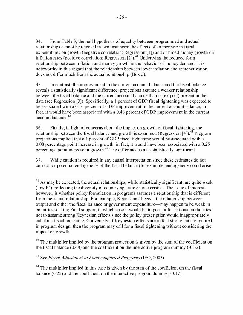
7. One approach to policy formulation would be for national authorities and Fund country teams to develop a comprehensive macroeconomic model linking policies to targets. This model could then be inverted to derive the policies necessary to achieve them. If the Fund was confident that the implied policies would be implemented, it would support a program that predicts that sufficiently ambitious targets would be achieved.

8. While such an approach would have a number of advantages—ensuring consistency, illustrating the effects of alternative policy mixes, and identifying intertemporal trade-offs between financing and adjustment—empirical and practical considerations make the use of comprehensive macroeconomic models implausible in most cases.4 Instead, therefore, national authorities and Fund country teams typically rely on a variety of approaches to help formulate macroeconomic and structural policies. For the purposes of discussion, it is useful to consider the process of policy formulation for short-run objectives (such as macroeconomic stabilization and external adjustment) separately from the longer-term goals of ensuring debt sustainability, reducing vulnerabilities, and raising the growth potential of the economy—though, of course, these are dynamically linked.

3 The objectives typically include promoting external adjustment and macroeconomic stability, of which restoring confidence in capital account crises is an extreme case; fostering growth and poverty reduction; and reducing vulnerabilities. These goals, of course, are not necessarily mutually exclusive—programs often aim at a number of objectives. The emphasis of the program, however, naturally depends upon country-specific circumstances; see Fund-Supported Programs: Objectives and Outcomes.

4 Experience with econometric models in industrialized countries suggests that parameter instability is a significant concern especially when policy changes are taking place (Lucas, 1976). This, together with a lack of data or ergodic time series in many countries supported by Fund arrangements, makes the stability of elaborate models suspect. Moreover, without ad hoc adjustments, it is difficult to capture the myriad of circumstance- and country-specific factors, some of which (e.g., the credibility of the program) do not lend themselves easily to formal modeling.

- 6 -

A. Macroeconomic Stabilization and External Adjustment

9. In formulating their economic program, national authorities have a number of different instruments—the exchange rate regime, monetary policy, fiscal policy, and structural measures. While such policy prescriptions would be consistent with most open-economy macroeconomic models, the specific policy content of the authorities’ program naturally depends upon the country’s characteristics and the circumstances it is facing. Thus, if Keynesian effects are likely to be important, then the effect of fiscal consolidation on activity and output growth would need to be taken into account. Likewise, the pace at which disinflation should be targeted—and the choice of nominal anchor—should be viewed against the benefits for growth of macroeconomic stability, the possible need to adjust administered prices in the economy, and realistic expectations regarding fiscal policy.5 Since no single model is universally applicable, national authorities—and Fund country teams in advising them—must draw on a smorgasbord of small econometric models and single equation estimates (including existing analytical work undertaken by research departments in central banks, ministries of finance, and private think tanks), as well as economic judgment for formulating macroeconomic and structural policies.

10. The program thus developed is essentially defined by a core set of macroeconomic projections on real GDP growth, inflation, the current account, and the balance of payments. In turn, these variables both influence, and are influenced by, monetary, exchange rate, and fiscal policy instruments. Thus inflation and growth will be important inputs into fiscal revenue and expenditure projections, but the size of the deficit may have a bearing on economic activity, and its financing on inflation and interest rates. Likewise, the monetary policy stance has implications for prices and output growth, but real growth, in turn, is likely to affect the demand for money.

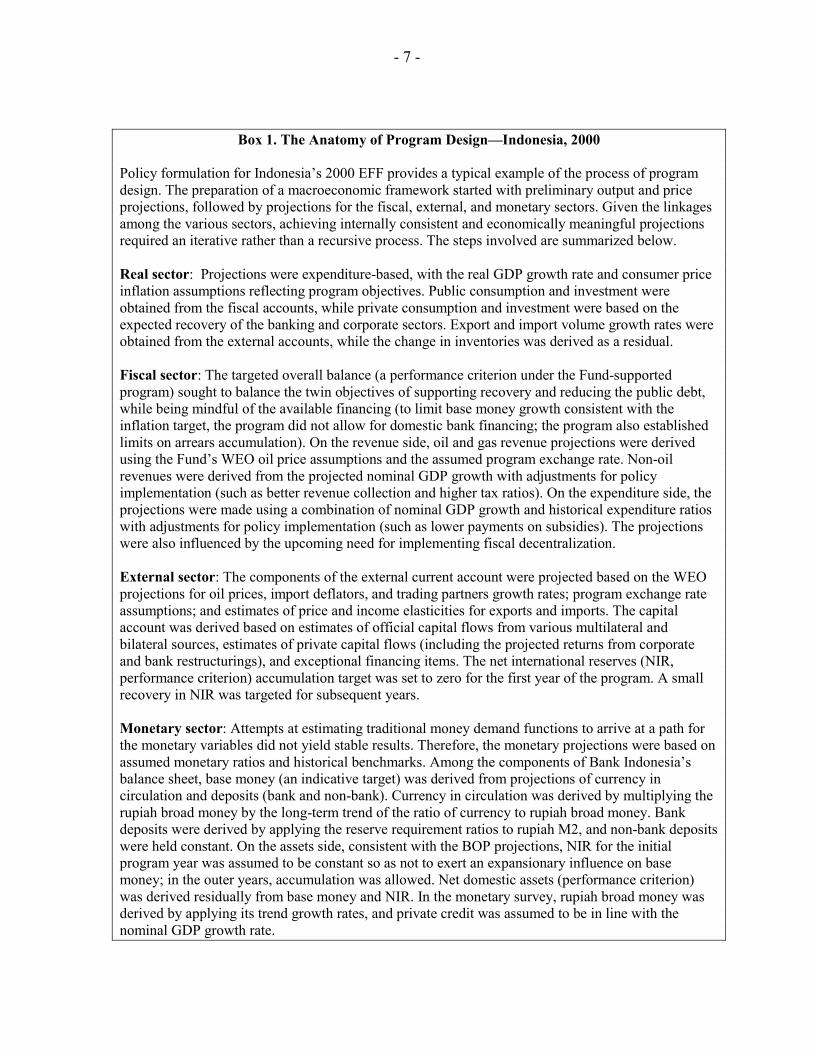
11. The mutual dependence of instruments and targets means that the modeling process is usually iterative and often quite complex (Box 1). A key concern is ensuring consistency of the macroeconomic framework and coherence of the policy stance across instruments to meet

5 Practical considerations may also constrain monetary and fiscal choices. For example, if the government is locked into high nominal interest rates on long maturity instruments, rapid disinflation—and high real interest rates—may be costly to the government. See Coorey et al. (1996) on accommodating administered price changes in inflation targets.

- 7 -

Box 1. The Anatomy of Program Design—Indonesia, 2000 Policy formulation for Indonesia’s 2000 EFF provides a typical example of the process of program design. The preparation of a macroeconomic framework started with preliminary output and price projections, followed by projections for the fiscal, external, and monetary sectors. Given the linkages among the various sectors, achieving internally consistent and economically meaningful projections required an iterative rather than a recursive process. The steps involved are summarized below. Real sector: Projections were expenditure-based, with the real GDP growth rate and consumer price inflation assumptions reflecting program objectives. Public consumption and investment were obtained from the fiscal accounts, while private consumption and investment were based on the expected recovery of the banking and corporate sectors. Export and import volume growth rates were obtained from the external accounts, while the change in inventories was derived as a residual. Fiscal sector: The targeted overall balance (a performance criterion under the Fund-supported program) sought to balance the twin objectives of supporting recovery and reducing the public debt, while being mindful of the available financing (to limit base money growth consistent with the inflation target, the program did not allow for domestic bank financing; the program also established limits on arrears accumulation). On the revenue side, oil and gas revenue projections were derived using the Fund’s WEO oil price assumptions and the assumed program exchange rate. Non-oil revenues were derived from the projected nominal GDP growth with adjustments for policy implementation (such as better revenue collection and higher tax ratios). On the expenditure side, the projections were made using a combination of nominal GDP growth and historical expenditure ratios with adjustments for policy implementation (such as lower payments on subsidies). The projections were also influenced by the upcoming need for implementing fiscal decentralization. External sector: The components of the external current account were projected based on the WEO projections for oil prices, import deflators, and trading partners growth rates; program exchange rate assumptions; and estimates of price and income elasticities for exports and imports. The capital account was derived based on estimates of official capital flows from various multilateral and bilateral sources, estimates of private capital flows (including the projected returns from corporate and bank restructurings), and exceptional financing items. The net international reserves (NIR, performance criterion) accumulation target was set to zero for the first year of the program. A small recovery in NIR was targeted for subsequent years. Monetary sector: Attempts at estimating traditional money demand functions to arrive at a path for the monetary variables did not yield stable results. Therefore, the monetary projections were based on assumed monetary ratios and historical benchmarks. Among the components of Bank Indonesia’s balance sheet, base money (an indicative target) was derived from projections of currency in circulation and deposits (bank and non-bank). Currency in circulation was derived by multiplying the rupiah broad money by the long-term trend of the ratio of currency to rupiah broad money. Bank deposits were derived by applying the reserve requirement ratios to rupiah M2, and non-bank deposits were held constant. On the assets side, consistent with the BOP projections, NIR for the initial program year was assumed to be constant so as not to exert an expansionary influence on base money; in the outer years, accumulation was allowed. Net domestic assets (performance criterion) was derived residually from base money and NIR. In the monetary survey, rupiah broad money was derived by applying its trend growth rates, and private credit was assumed to be in line with the nominal GDP growth rate.

- 8 -

program objectives. Financial programming is used as a general approach6 to inform and tie together the various sectors in a consistent manner, while incorporating country-specific factors.7 In this fashion, not only does financial programming serve as an ex ante consistency check on important financial aggregates, it also provides an ex post monitoring tool.8

12. A key characteristic of this approach is that it allows policies to be adjusted and re-formulated in a dynamic manner in the light of outcomes.9 Policy formulation thus extends well beyond the Board approval of a Fund arrangement. Indeed, program reviews are intended to offer the opportunity for country authorities and Fund staff to re-assess their initial assumptions and the progress achieved during the first few months of the program, including reasons why program objectives may be deviating from targets, with the forward-

6As noted in the text, the financial programming model is seldom used to pin down exact parameters of a program, but to inform and to help ensure consistency across sectors (external, monetary, fiscal). Specifically, the fiscal deficit must match sources of financing. These include: an external component, derived from an assessment of the balance of payments (at either a fixed exchange rate or an expected path of a floating exchange rate), the market’s appetite for sovereign bonds, external privatization receipts, and expected inflows through the banking system; expected privatization receipts; and government borrowing from the banking system. The latter is derived from assumptions regarding changes in broad liquidity, which in turn depend on money demand developments (given macroeconomic parameters such as growth and inflation), net foreign assets projections consistent with the BOP projections, and assumptions regarding net domestic claims on the private sector that are consistent with the growth projections.

7 See Polak (1957) and Robichek (1967, 1971). In its original conception, in a world of low capital mobility, limited recourse to bond financing by the government, and fixed exchange rates, the financial programming model was intended to define the fiscal deficit consistent with a reserves accumulation target. The assumptions underlying the “classic” financial programming model (see Appendix I; Mussa and Savastano, 1999) are unlikely to be fulfilled. These assumptions can be relaxed, however (Khan and Montiel, 1989).

8 The financial programming framework may therefore be useful for monitoring conditionality, serving as tripwires (ceilings or floors) for identifying instances in which a program is going off-track rather than for specifying the actual policy stance. In particular, the financial programming framework is not intended for setting monetary policy, which typically depends on the country’s monetary and exchange rate regime (e.g., a pegged exchange rate, a target for monetary aggregates, an inflation targeting framework, or an interest rate rule).

9 See Mussa and Savastano (1999).

- 9 -

looking aspect of Fund reviews allowing for policy adjustments to help ensure that program objectives are achieved.10

13. The need for frequent re-assessments of policies in light of outcomes is especially acute in capital account crises. Although these programs are, at one level, little different from more traditional programs—typically targeting some external adjustment (on average, about 1.1 percent of GDP; Table 1)—their salient feature is the large and sudden capital outflows that force much larger-than-envisaged adjustments of the current account balance (on average, 8.5 percent of GDP), with pervasive macroeconomic consequences.11 In particular, the timing and magnitude of the capital outflows are very difficult to predict—indeed, existing models of capital flows perform very poorly even in non-crisis situations.12 These flows and the attendant exchange rate movements interact with domestic balance sheet exposures, potentially altering the magnitude, and even the sign, of the effects of economic policies.13

10 While staff reports for program reviews usually analyze breaches of conditionality, they do not always analyze the reasons for deviations from broader program objectives.

11 A further complication in many capital crises were the concomitant banking crises.

12 Most models postulate that capital flows depend on relative expected returns. When capital mobility is high—as amongst industrialized countries—capital flows should respond immediately to any perceived differentials in expected rates of return, implying that uncovered interest rate parity (UIP) should hold continuously. In fact, however, empirical evidence suggests that deviations from UIP are pervasive and persistent. In comprehensive literature surveys, Froot and Thaler (1990) and MacDonald and Taylor (1992) report few cases where the interest rate differential has the right value or even the right sign.

13 For example, Furman and Stiglitz (1998) argue that monetary tightening may even produce a perverse effect on the exchange rate. In their view, tight monetary policies by causing widespread corporate bankruptcies can widen the risk premium, contributing to further outflows and depreciation of the exchange rate. The efficacy of tightened monetary policy in stemming capital outflows may therefore depend on the relative balance sheet exposures of the financial and corporate sector to exchange rate and domestic interest rate risk (see Montiel (2003) for a review of the empirical literature). Aghinon, Bacchetta, and Banerjee (2001) develop a model in which balance sheet effects alter the impact of monetary and fiscal policies on the economy. Likewise, the impact of fiscal policy may depend on parameters of the economy that may not be known at the time of a crisis (see IMF-Supported Programs in Indonesia, Korea, and Thailand (OP 178, Appendix 7.2) for a model in which the degree of capital mobility and balance sheet effects affect the impact of fiscal policy on output). IMF-Supported Programs in Capital Account Crises (OP 210) discusses how the appropriate response of fiscal policy depends on whether capital outflows represent a supply-side shock (for instance, because the exchange rate depreciation raises the cost of intermediate inputs or

(continued)

- 10 -

Table 1: Projected and Actual Current Account Adjustment in Capital Account Crisis Programs

(in percent of GDP)

Approval Crisis Current account adjustmentyear year Projected Actual

Argentina 2000 2002 0.1 12.0Brazil 1998 1999 0.6 -0.6Indonesia 1997 1998 0.5 6.0Korea 1997 1998 2.5 14.4Mexico 1995 1995 3.7 6.5Russia 1996 1999 0.0 12.1Thailand 1997 1998 2.0 14.8Turkey 1999 2001 0.3 7.2Uruguay 2000 2002 0.2 4.4

Average 1.1 8.5

Source: MONA and WEO databases, and staff estimates.

14. Partly in response, the Fund has been developing a balance sheet approach to understand the mechanisms underlying these stock shifts.14 From the perspective of this approach, a financial crisis occurs when a plunge in demand for financial liabilities takes place in one or more of the sectors—creditors may lose confidence in the sovereign’s ability to service its debt, in the banking system’s ability to meet deposit outflows, or in corporations’ ability to repay bank loans and other debt—ultimately spilling on to the balance of payments. Since most emerging market countries borrow in foreign currency, some sectors in the economy have foreign exchange risk. The key insight is that the maturity structure and distribution of those liabilities across domestic balance sheets, as well as the inter-relationships between balances among residents, may have important bearing on the country’s vulnerability to a shift in confidence. The balance-sheet analysis can help pinpoint

leads to widespread bankruptcies due to the corporate sector’s foreign exchange exposure) or a demand-side shock. Ultimately, there may be inherent limits to whether the effect of policies on macroeconomic targets can be knowable in crisis situations; such limits have long been recognized in the physical sciences—see Heisenberg (1927).

14 See The Balance Sheet Approach and its Applications at the Fund (SM/03/227); and Integrating the Balance Sheet Approach into Fund Operations (SM/04/52).

- 11 -

the source of balance of payments disequilibrium and, possibly, the form of intervention that might succeed in containing the crisis.

15. While a useful addition to the analytical toolkit, it is important to recognize the limitations of the approach. First, although it can help identify vulnerabilities, it cannot predict either the timing or the magnitude of a possible crisis and the capital outflows.15 Second, though some balance sheet structures may be more resilient than others, as long as the country as a whole has foreign exchange exposure, some balance sheet within the economy faces risks that cannot be diversified away. Finally, there are a number of difficulties in the practical application of the framework, particularly related to the availability of data.

B. Promoting Economic Efficiency and Output Growth

16. Enhancing economic efficiency and promoting growth are important goals of Fund-supported programs, particularly among low-income countries.16 Although the economics profession is far from reaching consensus on what drives growth, several conclusions emerge from various studies. First, most studies agree that macroeconomic stabilization is a sine qua non for sustained output growth and for reaping the benefits of any structural reforms, possibly because high and volatile inflation might lessen the value of price signals and distort the allocation of resources.17 Second, while there is less agreement on the best sequence for

15 Moody’s Macro Financial Risk Model (MfRisk) has applied the contingent claim analysis to the whole economy to estimate default and distress probabilities for the sovereign, the banking, and the nonfinancial corporate sectors. This approach is forward-looking in that it uses the information contained in financial asset prices to predict default probabilities, while the balance sheet approach relies on past financial statements. Moody’s MfRisk model also assesses risk transfers from one sector to another (see Gapen et al., 2004). While the model’s main application to date has been in the corporate and financial sectors, which are particularly amenable to statistical methods given large samples of data, it is also being used by institutional investors and investment banks to model sovereign risk. 16 PRGF-supported programs also target poverty reduction; some of these measures, including improving health and education, are likely to have positive growth effects as well.

17 Most empirical work finds a negative and convex relationship between inflation and growth. The greatest marginal loss of growth occurs at low inflation rates—beyond a low inflation “kink’ that studies place variously between about 3 and 8 percent per year (see Sarel (1996), ESAF Review (1997), and Ghosh and Phillips (1998)). Beyond the kink point, each doubling of the inflation rate is associated with ½ percentage point lower per capita growth. As usual there are caveats regarding causal interpretations—and high inflation may be capturing macroeconomic dislocation more generally—but the relationship is surprisingly robust to controls for endogeneity and the inclusion of other growth determinants. Evidence

(continued)

- 12 -

reforms, a widely accepted view is that stabilization should precede trade18 or financial sector19 liberalization, particularly if these can adversely affect stabilization efforts by reducing trade-related revenues or raising the costs of public sector funding. Moreover, domestic financial markets should be liberalized—with well-supervised prudential regulations in place—before the capital account to ensure an efficient allocation of resources and to limit vulnerabilities. Third, a growing body of literature emphasizes the importance of sound institutions for sustained output growth. At the same time, the variety of judicial systems and institutions in strong performing economies belies the idea that any single approach works best in all countries.20

17. Beyond these general prescriptions, there are four main analytical tools for understanding the determinants of activity and output growth. First is the demand side assessment—that is, a decomposition of the expected growth into private consumption, investment, government spending, and the current account balance. While this does not provide a model of potential output, it does provide a check on whether the growth projection is consistent with other program parameters, for instance fiscal adjustment. Second, mechanical univariate approaches, such as HP filters, may be useful input to medium-term growth projections.21 Third, estimating the aggregate production function may also serve to model growth and discipline projections. However, even though this provides a model for potential output growth, it requires data that is not readily available (e.g., capital stock data) as well as assumptions regarding competition in factor markets or estimates of factor utilization; of course, growth of potential output need not translate into actual output growth if demand is lacking or economic inefficiencies abound. Fourth, growth regressions can be

on sequencing of reforms presented in Zalduendo (2004) suggests that macroeconomic stabilization is so critical for economic performance that it is a pre-condition for deriving positive results from structural reforms.

18 Many authors argue that trade barriers should be dismantled only if alternative revenue sources have been identified (Funke (1993), and Nsouli et al. (2002)). Michaely et al. (1990) argue that the benefits of trade liberalization weaken if fiscal imbalances result in a real exchange rate appreciation that erodes the incentive of moving resources to the tradables sector. Others call for the implementation of trade reforms that do not affect the inflation rate—e.g., shifting from quantitative restrictions to tariffs (Krueger, 1984).

19 The timing of financial liberalization should also depend on a country’s initial conditions; e.g., whether financial repression is used to help finance the public sector.

20 Mauro (1995), Kaufman, Kraay, and Zoido-Lobatón (1999), and WEO (2003).

21 Peak-to-peak (and trough-to-trough) growth developments can help inform projections of potential growth. These tools do not, however, assess determinants of growth and frequently have difficulty in distinguishing between trend and one-time factors.

- 13 -

used to map country characteristics (including the availability of factors of production, such as physical and human capital, and structural characteristics, economic policies, and institutions) into its expected growth performance based on cross-country experience. Such regressions perform best over medium-term horizons—usually a five-year period—where business-cycle movements and the effects of temporary shocks are averaged out. Their major drawbacks are their data requirements, and the inherent difficulties of quantifying some of the explanatory variables, such as the quality of institutions. One approach would be to examine the association between growth and specific measures in similar (possibly neighboring) countries. These comparisons could usefully include data on medium-term growth rates in countries that are facing similar challenges and are situated at similar stages of development, which in turn would serve to further discipline projections.

18. A growth model would also allow an assessment of whether the assumed acceleration in growth is realistic and whether the structural reforms embodied in the authorities’ reform program could plausibly lead to such an acceleration. At the same time, it needs to be recognized that it is enormously difficult to map specific measures into the structural indices typically employed in growth regressions. Moreover, while the authorities may draw on cross-country experience to identify broad areas where reforms could bolster growth, they must rely on their own country-specific knowledge to determine the growth bottlenecks that are critical for their country. Even when there is agreement on which reforms might contribute to better economic performance, a further difficulty lies in determining the impact of these reforms on growth—specifically, whether the beneficial effects are likely to peter out quickly or to have a lasting effect on a country’s growth performance. Empirical research suggests that various economic measures—macroeconomic stability, an enabling business environment, trade liberalization, fiscal sustainability, and financial sector development—boost output growth, but in some cases—such as trade liberalization and fiscal sustainability—the long-run effect on the growth rate is weaker (Box 2). It would therefore be important to distinguish between immediate and lasting effects on growth rates in assessing the impact of structural reforms on the country’s growth performance.

19. Despite the availability of these analytical tools, and notwithstanding their shortcomings, a review of a sample of staff reports over a 6-year period shows that they typically make limited use of these tools (9 out of 20 staff reports used one or another of the above described techniques, and in almost all cases only once over the 6-year period; see Box 3). As discussed below, greater use of analytical tools could discipline medium-term growth projections embodied in programs as well as helping to identify some of the impediments to growth pertinent to the particular country.

- 14 -

Effects on Growth Rates

Coefficient Standard Annualdeviation growth

effectBusiness environment 0.04 0.14 0.51Financial sector development 0.02 0.16 0.28Economic stabilization 0.06 0.07 0.42Trade liberalization 0.07 0.07 0.49Fiscal sustainability 0.07 0.08 0.58

Growth Effects 1/(Dependent variable: Growth rate in GDP per capita)

Number of observations 172Number of different countries 61

Equation 1 Equation 2 Equation 3

Economic policy regressorsBusiness environment 0.0359 *** 0.0717 ***

3.40 4.44Financial sector development 0.0177 *** 0.0248 ***

2.91 3.47Economic stabilization 0.0639 *** 0.0920 ***

4.17 4.34Trade liberalization 0.0652 *** 0.1552 ***

3.67 4.19Fiscal sustainability 0.0720 *** 0.1108 ***

4.33 6.03Business environment, lagged 0.0097 -0.0442 ***

0.99 -2.96Financial sector development, lagged 0.0067 -0.0050

1.55 -0.60Economic stabilization, lagged 0.0680 ** -0.0004

2.54 -0.01Trade liberalization, lagged 0.0525 *** -0.0998 ***

5.10 -2.73Fiscal sustainability, lagged 0.0125 -0.0527 ***

0.94 -3.11Wald statistic 191.57 204.55 271.63Standard error of regression 0.0213 0.0230 0.0208R-squared 0.43 0.32 0.45*** indicates significance at 1 percent; ** indicates significance at 5 percent1/ Regression includes a number of non-policy regressors, such as initial income level,terms of trade shocks, and indicators of domestic shocks. Some of these regressorsserve to control for differences in initial conditions.

Box 2. Permanent and Temporary Growth Effects from Economic Policies

A cross-country growth equation representing five clusters of economic policies suggests that improving each of these clusters by one standard deviation leads to improvements in growth rates that range from 0.3 to 0.6 percent per year (see Zalduendo, 2004) for a discussion of the use of the cluster approach to capturing different dimensions of economic policy. The five clusters were derived by applying factor analysis to different economic policy indicators. These empirical results use an unbalanced panel of 5-year periods between 1981 and 2000. The two clusters of macroeconomic policy are viewed as proxies to economic stabilization and fiscal sustainability. The three clusters of reforms represent trade liberalization policies, financial sector development, and an enabling environment for private sector activity.

Is the growth pay-off from a given improvement in economic policies permanent? The econometric results suggest that growth effects from sound policies are lasting, but that some policies have a more lasting impact than others. This conclusion is derived by comparing three regressions. The first regression includes only contemporaneous measurements of economic policy clusters. The second regression includes only lagged indicators (i.e., the average of the preceding 5-year period). The last regression combines contemporaneous indicators and the lagged 5-year period for each economic policy regressor. The coefficient estimates in the first equation are positive (better policies support growth) and statistically significant. The conclusions from the second equation are similar, albeit less robust—only lagged macroeconomic stabilization and trade liberalization are statistically important for growth. In contrast, the last equation has positive coefficient estimates on contemporaneous indicators of policy clusters and negative estimates in the lagged indicators. While the sum of the corresponding statistically significant contemporaneous and lagged coefficients is still positive, it is weaker than the contemporaneous effect by itself. More precisely, the combined contemporaneous and lagged coefficients for trade liberalization and fiscal sustainability (equation 3) are smaller than those in the specification that has only contemporaneous regressors (equation 2). In sum, even though the observed growth effects are lasting, in some cases they weaken over time.

- 15 -

Box 3. The Treatment of Growth in Staff Reports—Theory and Practice

Even though growth projections are not intended to be forecasts (they are conditioned, inter alia, on policy implementation, and reflect a mix of quantitative analysis and judgment reached during discussions between country authorities and Fund staff), the existence of systematic biases are problematic because they provide a poor basis for choosing the macroeconomic policies and distort the assessment of debt sustainability.

What options are available when preparing growth projections?

The options depend on the length of the projection period and the availability of data. One-time factors, sector-specific issues, and cyclical factors play an important role when preparing short-term growth projections. Unfortunately, many of these factors do not lend themselves easily to formal modeling. A detailed demand-side analysis also provides a useful perspective when preparing growth projections. The range of options broadens for medium-term projections: mechanical univariate approaches (HP-type filters), production function approaches, and growth equations. However, these options also have limitations. Univariate-based assessments have difficulty in distinguishing between trend and one-time factors. Production function approaches are intensive on data that is frequently not available, such as capital stock data, or based on accounting exercises that depend heavily on assumptions regarding factor utilization and production function parameters. Growth equations lack a theoretical foundation. An additional difficulty relates to the quantification of the effects of structural reforms on growth. In fact, it is fair to say that individual reforms might have a limited effect on output. More likely, it is the accumulation of sound economic management and structural reforms that strengthens a country’s growth prospects.

A review of selected Fund reports (twenty staff reports for Article IVs and UFR programs, as well as selected issues papers) covering the period 1995-2000 reveals that:

• almost half of the reports utilized at least once during the 6-year period an analytical framework for growth projections—HP filters and ICOR relationships were the most frequently employed techniques;

• on slightly over half of the sample analytical work was not feasible or not explicitly described in the reports;

• links between reforms and growth are rarely analytical, perhaps reflecting the quantification difficulties mentioned above;

• most reports provide a demand-side assessment based on a S-I discussion, though these assessments are not always fully explained;

• commodity-based countries provide a supply-side analysis (weather and positive shocks); and

• other supply side assessments refer to sector-specific factors, such as developments in the oil sector.

Year HP Growth Otherfilter equation Growth

acctg.Deriv. of

PF

Argentina 1996 xArmenia 1996 x 1/Central African Rep. 1998 x 1/Congo 1996 x 2/Cote d'Ivoire 1998 x 3/Ghana 1999 x 1/Guinea Bissau 1995 x 3/Guinea Bissau 2000 x 1/Guyana 1998 x 4/Jordan 1998 xKenya 2000 xKyrgyz 2000 x x xMacedonia, FYR 1997 x 1/Madagascar 1996 x 3/Malawi 2000 x 1/Niger 2000 x 2/Philippines 1999 x x xSenegal 1998 x 1/Vietnam 1999 xZambia 1995 x 1/

3/ Based on ICOR assumptions.

1/ Ad hoc (e.g., increase savings and investment through program reforms).

4/ Report mentions rise in productivity, though no model is discussed.

Use of Analytical Growth Frameworks

Prod. Function (PF)

Sources: EBS and SM reports, 1995-2000.

2/ Underlying population growth and total productivity assumptions.

- 16 -

C. Medium-term Debt Sustainability

20. An important use of medium-term growth projections is to inform debt sustainability assessments. Indeed, going beyond flow balance of payments problems, Fund-supported programs are also intended to reduce vulnerabilities to future crises so that a country should emerge with both its public and external debt dynamics on a sustainable path. To assess debt dynamics, the Fund has developed a standardized debt sustainability template.22 The template lays bare the key assumptions underlying the debt sustainability analysis so that their realism can be assessed against a country’s historical experience. The template also applies stress tests to the baseline projection to examine its resilience to shocks and serves to anchor near-term policy recommendations.

21. Some of the debt sustainability template’s features and limitations are also worth noting, however.23 First, the template articulates debt dynamics under the baseline and stress scenarios, and thus helps arrive at judgments about the sustainability of a given path of debt, but cannot replace the need for such judgments. Second, the template is intended to take account of the main shocks—such as poor growth performance or real exchange rate depreciations—that could result in an unsustainable increase in debt, but not to model the crisis itself. Thus, while the template tracks gross financing needs, it is not well-suited to modeling how liquidity crises manifest since it focuses only on the country’s aggregate net external debt and capital flows. Third, although the template helps discipline projections, it does not specify a particular model or method that country teams should use in making program projections; ultimately, debt sustainability assessments will only be as good as the macroeconomic projections, including for output growth, underlying it.

III. PERFORMANCE OF ANALYTICAL FRAMEWORKS AND PROGRAM DESIGN

22. The preceding discussion outlined the processes and analytical tools that national authorities—and Fund country teams in advising them—use to formulate policies in Fund-supported programs. This section seeks to examine how well these tools perform in practice, with a view to assessing the performance of the modeling process rather than evaluating the outcomes of programs.24 Since this is difficult to do directly—and since a program is in

22 The debt sustainability template (SM/02/166 and SM/03/206) was designed for market borrowers; a similar framework, taking account of factors specific to low-income countries, was approved for analytical work by the Executive Board (SM/04/27, March 2004).

23 See SM/03/206 for a discussion of the issues that arise in the practical application of the template; for instance, choosing the appropriate window of historical data for the calibration of shocks is particularly difficult when countries are undergoing rapid structural change.

24 Outcomes and experience with Fund-supported programs are discussed in greater detail in the companion papers on Fund-Supported Programs—Objectives and Outcomes and

(continued)

- 17 -

essence defined by its intended outcomes—the tack taken here is to examine whether there are systematic errors in projections for key objectives, including real GDP growth, inflation, and the current account balance (Section A).

23. An important question is the horizon over which such projections should be assessed. On the one hand, most countries set budgets annually (though there may be supplemental budgets).25 On the other hand, in Fund-supported programs, policies (and particularly program targets) are seldom set for more than one or two quarters ahead without at least some opportunity to reconsider them, in light of developments, at the time of the quarterly or semi-annual program reviews. This suggests that, for assessing the analytical underpinnings of policy formulation, short horizons of one year or less (referred to as year t) are the most relevant, which in turn are affected by what is known regarding period t-1.26 In this regard, the deviations between estimates and actuals in year t-1 show that both GRA- and PRGF-supported programs underestimate growth (Box 4). The current account balance is also underestimated in GRA-supported programs in spite of the overestimation of the fiscal balance, while the opposite is the case among PRGF-supported programs. Although, on average, these deviations are generally not statistically significant, their magnitude (as measured by the root mean squared error) suggests that policy settings and projections for the program period might have been different had the assessment of prevailing economic conditions been more accurate.

24. Examining projection errors for the year following program approval (t+1) is also important inasmuch as they capture whether the program’s broad objectives are being met, even if there may be an opportunity to adjust policies in light of evolving developments afterwards. The evidence on projection errors mingles the effects of modeling errors, exogenous shocks, and, possibly, uneven (or even no) policy implementation. For the purposes of policy formulation, however, it is important that national authorities and country teams understand the relationships between macroeconomic policies and program objectives. In this regard, identifying appropriate corrective measures requires understanding whether targets were missed because of modeling errors, exogenous shocks, or policy slippages. In addition, even if projection errors turn out to be small, knowing how to adjust

Macroeconomic and on Structural Policies in Fund-Supported Programs—Review of Experience.

25 Some countries prepare medium-term budget frameworks, typically covering three-year periods, but these are often mainly indicative—much of the focus of economic policies is on the budget for the upcoming fiscal year.

26 As noted above, a key component of program design is the scope for introducing adjustments to program targets and policies at the quarterly and semi-annual reviews.

- 18 -

Box 4. Impact of Data Revisions for Year t-1 Estimates of previous years’ outturns are preliminary at best when authorities are formulating their economic policies. In turn, different initial conditions might call for different policy choices.1 How large are data revisions in practice? The text table provides the average deviations (and standard deviations) of some key macroeconomic variables across program types between the revised (actual) data and the original program estimates for period t-1. The main results that emerge are: real GDP growth in the previous period is underestimated across all program types by over ¼

percent—however, this under estimation is not statistically significant; the current account balance is underestimated by about a ½ percentage point of GDP in GRA-

supported programs (i.e., the deficit outturn in t-1 is smaller than estimated), but overestimated by ¾ percentage point in PRGF-supported programs—the former is statistically significant while the latter is not; and the overall fiscal balance in GRA-

supported programs was overestimated by 0.4 percentage points of GDP (i.e., the deficit in t-1 turns out to be larger than considered at the time of the program approval), while the fiscal balance deviation in PRGF-supported programs was underestimated by about the same amount—neither is statistically significant. Data revisions, even if not statistically significant, might have modified policy setting. Furthermore, the projections for periods t and t+1 are also likely to have been different if the actual t-1 data were available at the time of program design, which could possibly reduce the projection errors. _________________________ 1 For a discussion, see Morgenstern (1950).

policies in light of evolving developments requires an understanding of the underlying macroeconomic model. Section B, therefore, examines whether systematic biases exist in the relationships between macroeconomic policies and targets being assumed.

25. While near-term projections are the most relevant for formulating the appropriate macroeconomic policy response, member countries should also emerge from their Fund-supported programs with sustainable external debt positions.27 Such assessments require a 27 Indeed, Fund resources cannot be provided if the country’s external debt is not expected to be sustainable.

t-1 RMSE

Real GDP growth 0.29 3.28EFF/SBA 0.31 4.01SAF/ESAF/PRGF 0.26 1.94

Current account balance (% of GDP) -0.07 2.51EFF/SBA 0.46 * 1.80SAF/ESAF/PRGF -0.74 3.09

Overall fiscal balance (% of GDP) 0.00 3.99EFF/SBA -0.40 4.65SAF/ESAF/PRGF 0.40 2.96

Sources: MONA, WEO, and staff calculations.1/ Actual minus program estimate* implies t-statistic significant at the five percent level.

Average Deviations 1/(In percentage points)

- 19 -

longer horizon and corresponding projections for the evolution of the external balance, real exchange rates, and output growth. These are examined in Section C.

A. Near-Term Macroeconomic Projections

Output Growth

26. On the whole, near-term projections in Fund-supported programs—reported in Table 2—are relatively good. In GRA-supported programs, excluding a handful of capital account crisis programs, the average bias in year t was not statistically significant (Figure 1, top panel).28 In contrast, for capital account crisis cases, growth rates were over-predicted—on average 9¼ percentage points, a statistically significant bias. In PRGF-supported programs, growth in the year of program approval is over-predicted by 0.4 percentage points per year—a magnitude that is insignificant in relation to the volatility of growth (Figure 1, bottom panel).29 Indeed, the root mean squared error (RMSE) of the projection is 2¼ percent per year against a standard deviation of growth of 2¾ percent per year.30

27. At the one-year horizon (i.e., growth between the year of program approval, t, and the next year, t+1) growth projections do not fare as well. The bias among PRGF-supported programs is about 1.2 percentage points, a statistically significant error with a RMSE of 3.1 percentage points per year. For GRA-supported programs, the bias increases to 0.7-0.9 percentage points, though these errors remain not statistically significant. Moreover, errors are serially correlated, implying that countries for which growth is over-predicted in one year are more likely to be over-predicted the following year as well.

28. These findings could reflect the tension that arises from using real GDP growth both as a key variable that requires realism for program design purposes and as a political objective.31 Yet, empirical evidence suggests that upward biases are no larger when a

28 This result is consistent with the findings of Musso and Phillips (2001).

29 For programs approved in the fourth quarter of year t, this projection refers to year t+1. In practice, given the time required for program discussions, the outturn for the first quarter may not even be available during negotiations of an arrangement approved at mid-year.

30 The root mean squared error (RMSE) gives a measure of how large is the typical error without allowing for positive and negative errors across programs to cancel out each other.

31 This may be particularly pertinent in low-income countries, where overly conservative growth projections may be interpreted as constraining countries’ development potential.

- 20 -

Table 2: Statistical Characteristics of Program Projection Errors 1/

Number Period t Period t+1 ρ (error t ; error t+1)obs. Mean RMSE Mean RMSE

error error

Real GDP Growth

PRGF-supported programs 56 -0.4 2.2 -1.2 *** 3.1 0.49 ***GRA-supported programs

Transition 2/ 27 0.1 3.7 -0.7 4.4 0.65 *** Non-transition 2/ 35 -0.3 2.7 -0.7 4.4 0.37 ** CACs 3/ 9 -9.3 *** 10.7 -0.9 5.0 -0.13

Inflation

PRGF-supported programs 47 0.9 8.1 4.0 ** 13.0 0.59 ***GRA-supported programs

Transition 2/ 21 0.3 12.6 5.4 16.5 0.52 ** Non-transition 2/ 25 1.5 12.4 1.8 11.5 -0.29 CACs 3/ 6 16.1 19.7 4.9 8.6 -0.08

Current Account Balance

PRGF-supported programs 48 -1.5 ** 4.9 -1.9 *** 4.8 0.64 ***GRA-supported programs

Transition 2/ 24 0.4 2.5 -0.4 2.3 0.15 Non-transition 2/ 28 2.4 *** 4.6 2.7 *** 5.2 0.79 *** CACs 3/ 8 5.6 ** 7.2 6.5 ** 8.7 0.62 *


* = significant at 10% level, ** = significant at 5% level, *** = significant at 1% level .

1/ Data transformed so that it maps into the interval (-100, 100). Errors defined as actuals minus projections.Table constructed using a dataset of countries with available information for year t, t+1, t+2, and t+3.2/ Excludes capital account crises.3/ CAC stands for capital account crises.

- 21 -

Figure 1. Real GDP Growth, Projections and Actuals(X-axis projections; Y-axis actuals)

Source: WEO and MONA databases, and staff estimates.Note: Data mapped into the interval (-100, 100).* Capital account crisis countries are depicted by triangles.

GRA-Supported in period t *

-15

-10

-5

0

5

10

15

-15 -10 -5 0 5 10 15

GRA-Supported in period t+1 *

-15

-10

-5

0

5

10

15

-15 -10 -5 0 5 10 15

GRA-Supported, average(t+1:t+3) *

-15

-10

-5

0

5

10

15

-15 -10 -5 0 5 10 15

PRGF-Supported in period t

-8

-4

0

4

8

12

-4 0 4 8 12

PRGF-Supported in period t+1

-8

-4

0

4

8

12

-4 0 4 8 12

PRGF-Supported, average (t+1:t+3)

-8

-4

0

4

8

12

-4 0 4 8 12

45 degree

line

45 degree

line

45 degree

line

45 degree

line

45 degree

line

45 degree

line

member has a Fund-supported program than when it does not.32 In addition, given that these growth projections are predicated on the full implementation of the authorities’ intended policies, some optimistic bias could be expected.

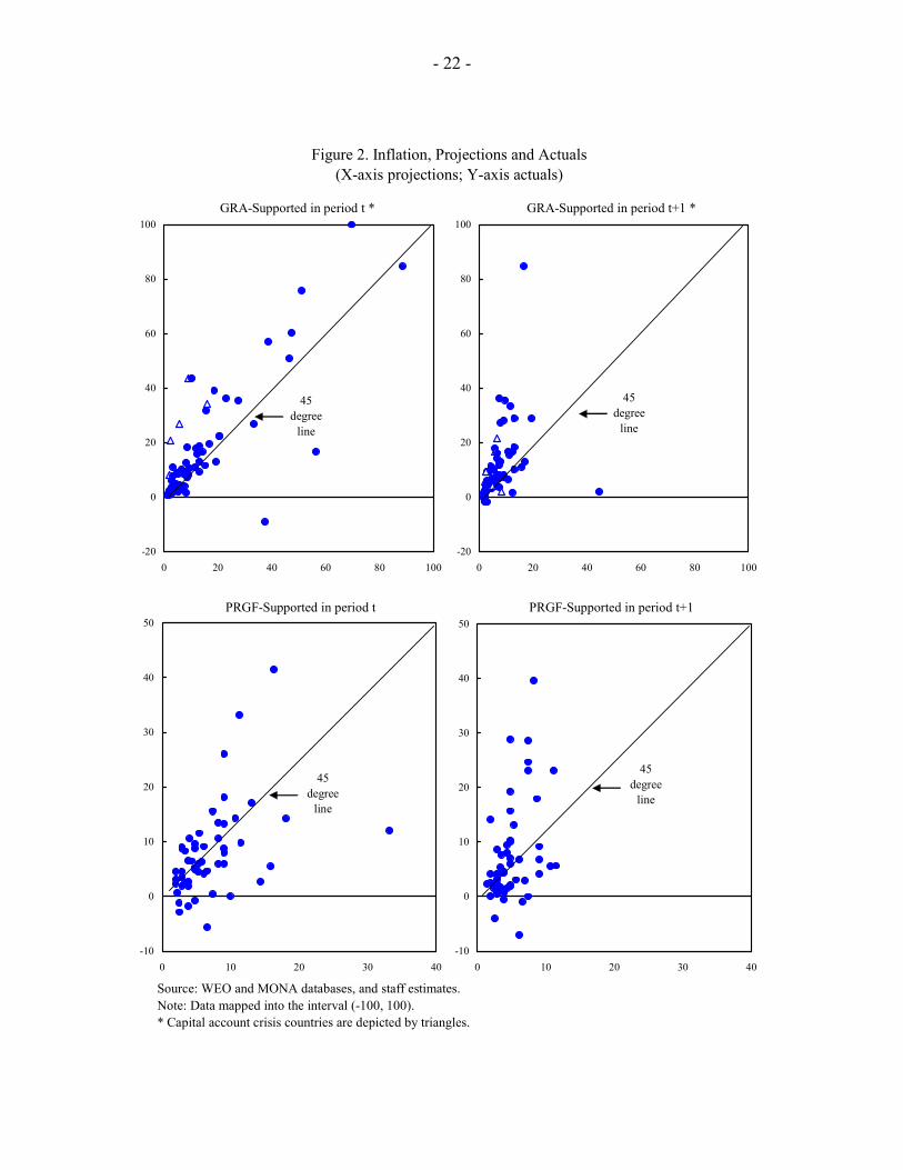
Inflation

29. Inflation tends to be underpredicted in the year of program approval, but this bias is not statistically significant (Figure 2).33 More precisely, inflation in the year of program approval is, on average, under-predicted by 1 percentage point per year in PRGF-supported programs and by a similar margin in GRA-supported programs (transition and non-transition combined, excluding capital account crises), but neither of these deviations is statistically

32 See Joshi and Ghosh (2003) for an analysis using projections undertaken for the World Economic Outlook (WEO) exercise (see also WEO, May 1996).

33 The dataset is mapped into the interval (-100, 100) to reduce the incidence of outliers.

- 22 -

Figure 2. Inflation, Projections and Actuals(X-axis projections; Y-axis actuals)

Source: WEO and MONA databases, and staff estimates.Note: Data mapped into the interval (-100, 100).* Capital account crisis countries are depicted by triangles.


-20

0

20

40

60

80

100

0 20 40 60 80 100


-20

0

20

40

60

80

100

0 20 40 60 80 100


-10

0

10

20

30

40

50

0 10 20 30 40


-10

0

10

20

30

40

50

0 10 20 30 40

45 degree

line

45 degree

line

45 degree

line

45 degree

line

- 23 -

significant. Among capital account crises, projection errors average 16 percentage points (while the error among capital account crises is large, it is not statistically significant, mainly on account of the small number of observations).34

30. Projection errors for inflation in the year following program approval tend to be much larger―except among capital account crises countries―and, once again, under-predicted.35 However, only the projection errors in PRGF-supported programs are statistically significant. The deviations may reflect unrealistic targets for disinflation rather than genuine projection errors owing in part to the tension between the realism of projections and the highly political role played by some of these economic indicators. Although the projection errors are serially correlated in PRGF-supported programs (with a statistically significant coefficient), they are generally not correlated in the GRA sample (except in transition economies).


31. Among GRA-supported countries, the current account in the year of program approval turns out to be stronger than expected (a larger surplus or a smaller deficit)—by about 2½ percent of GDP among non-transition economies, which is a statistically significant difference (Figure 3). These projection errors are particularly large, of course, for capital account crises. The comparable projection error for transition economies was not statistically significant. Among PRGF-supported programs, by contrast, current account deficits are larger than projected—by about 1½ percentage points of GDP.36 In fact, statistically significant biases are recorded in the first few years that follow the implementation of a Fund-supported program. Projection errors are also serially correlated—if adjustment is over-predicted in one year, it is likely to be over-predicted in the following year.

B. Actual and Programmed Relationships between Policies and Targets

32. As noted above, projection errors for key macroeconomic variables potentially mix a number of different effects—modeling errors, exogenous shocks, and weak policy

34 The RMSEs are also large, ranging from 8 percentage points in PRGF-supported programs to 12½ points in GRA-supported programs (and about 20 points in capital account crises).

35 See Macroeconomic and Structural Policies in Fund-supported Programs: Review of Experience for a discussion of the reasons why inflation diverged from program targets.

36 See Fund-supported Programs: Objectives and Outcomes for a discussion of the contrasting external adjustment patterns in GRA- and PRGF-supported programs.

- 24 -

Figure 3. Current Account Balance, Projections and Actuals(X-axis projections; Y-axis actuals)

Source: WEO and MONA databases, and staff estimates.* Capital account crisis countries are depicted by triangles.


-20

-15

-10

-5

0

5

10

15

20

-20 -15 -10 -5 0 5


-20

-15

-10

-5

0

5

10

15

20

-20 -15 -10 -5 0 5


-40

-30

-20

-10

0

10

-40 -30 -20 -10 0 10


-40

-30

-20

-10

0

10

-40 -30 -20 -10 0 10

45 degree

line

45 degree

line

45 degree

line

45 degree

line

- 25 -

implementation.37 Program documents, however, seldom articulate explicitly the underlying framework (they simply report projections for macroeconomic variables), thus making it difficult to test whether the framework itself is correct. The approach taken here, therefore, is to consider whether the relationships between policies and targets (fiscal balance and growth; fiscal expenditures and growth; fiscal balance and the current account balance; and money growth and inflation) implicitly assumed in programs are consistent with the actual (ex post) relationships. It bears emphasizing that the issue of interest here is the bivariate interaction between the variables (for instance, the fiscal balance and growth), without any causal interpretation; as such, econometric simultaneity is not a concern.

33. Specifically, to test whether programmed and actual relationships differ, a bivariate regression was estimated (for instance, between the fiscal balance and output growth) on data for both actual and programmed variables, with an interactive dummy to distinguish those observations that pertain to the programmed relationship.38 If this interactive dummy is statistically significant, then the relationship (say, between the fiscal balance and output growth) assumed in programs differs significantly from the actual relationship.39 Controls are added for the type of Fund-supported program and other group-specific characteristics (such as capital account crisis and transition economy programs); these allow for the different average projection errors identified above.40

37 If the target, y, is a function of policies, x, other variables, z, and a random shock, ε : y x zα β γ ε= + + + , then the projection error can be written: $ $ $ $( ) ( ) ( ) ( ) ( )

model error policy slippage shock

y y x z x x z zα α β β γ γ β γ ε− = − + − + − + − + − +$ $1444442444443 14243 14243

. The analysis in Section A

considered the full program projection error ( $y y− ), while this Section focuses on whether the analytical frameworks employed in program design get the policy multipliers, ( ˆβ β− ), right. Macroeconomic and Structural Policies in Fund-Supported Programs—Review of Experience examines the role of policy implementation in accounting for slippages in targets. See also Baqir, Ramcharan, and Sahay (2004).

38 An alternative approach would be to estimate these regressions separately for programmed and actual data and use a Wald test statistic to test for the equality of the relationships across the two samples.

39 These relationships pertain to variables in the year of program approval (or the following calendar year for programs approved in the fourth quarter) and year t+1.

40 For example, in the current account balance regression, the dummy corresponding to PRGF-supported programs is negative, reflecting the lower-than-projected external balances in these countries. Conversely, the capital account crisis dummy is positive, reflecting the greater-than-programmed current account adjustment.

- 26 -

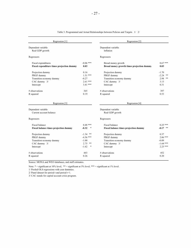
34. From Table 3, the null hypothesis of equality between programmed and actual relationships cannot be rejected in two instances: the effects of an increase in fiscal expenditures on growth (negative correlation; Regression [1]) and of broad money growth on inflation rates (positive correlation; Regression [2]).41 Underlying the reduced form relationship between inflation and money growth is the behavior of money demand. It is noteworthy in this regard that the relationship between lower inflation and remonetization does not differ much from the actual relationship (Box 5).

35. In contrast, the improvement in the current account balance and the fiscal balance reveals a statistically significant difference; projections assume a weaker relationship between the fiscal balance and the current account balance than is (ex post) present in the data (see Regression [3]). Specifically, a 1 percent of GDP fiscal tightening was expected to be associated with a 0.16 percent of GDP improvement in the current account balance; in fact, it would have been associated with a 0.48 percent of GDP improvement in the current account balance.42

36. Finally, in light of concerns about the impact on growth of fiscal tightening, the relationship between the fiscal balance and growth is examined (Regression [4]).43 Program projections implied that a 1 percent of GDP fiscal tightening would be associated with a 0.08 percentage point increase in growth; in fact, it would have been associated with a 0.25 percentage point increase in growth.44 The difference is also statistically significant.

37. While caution is required in any causal interpretation since these estimates do not correct for potential endogeneity of the fiscal balance (for example, endogeneity could arise

41 As may be expected, the actual relationships, while statistically significant, are quite weak (low R2), reflecting the diversity of country-specific characteristics. The issue of interest, however, is whether policy formulation in programs assumes a relationship that is different from the actual relationship. For example, Keynesian effects—the relationship between output and either the fiscal balance or government expenditure—may happen to be weak in countries seeking Fund support, in which case it would be important for national authorities not to assume strong Keynesian effects since the policy prescription would inappropriately call for a fiscal loosening. Conversely, if Keynesian effects are in fact strong but are ignored in program design, then the program may call for a fiscal tightening without considering the impact on growth.

42 The multiplier implied by the program projection is given by the sum of the coefficient on the fiscal balance (0.48) and the coefficient on the interactive program dummy (-0.32).

43 See Fiscal Adjustment in Fund-supported Programs (IEO, 2003).

44 The multiplier implied in this case is given by the sum of the coefficient on the fiscal balance (0.25) and the coefficient on the interactive program dummy (-0.17).

- 27 -

Table 3. Programmed and Actual Relationships between Policies and Targets 1/ 2/

Regression [1] Regression [2]

Dependent variable Dependent variableReal GDP growth Inflation

Regressors Regressors

Fiscal expenditures -0.06 *** Broad money growth 0.67 ***Fiscal expenditure times projection dummy 0.03 Broad money growth times projection dummy 0.03

Projection dummy 0.16 Projection dummy -1.70PRGF dummy 1.51 *** PRGF dummy -2.24 **Transition economy dummy -0.27 Transition economy dummy 2.98 **CAC dummy 3/ 2.61 *** CAC dummy 3/ 3.13Intercept 3.41 *** Intercept 0.31

# observations 365 # observations 397R squared 0.19 R squared 0.53

Regression [3] Regression [4]

Dependent variable Dependent variableCurrent account balance Real GDP growth

Regressors Regressors

Fiscal balance 0.48 *** Fiscal balance 0.25 ***Fiscal balance times projection dummy -0.32 * Fiscal balance times projection dummy -0.17 **

Projection dummy -1.34 ** Projection dummy 0.37PRGF dummy -4.56 *** PRGF dummy 2.06 ***Transition economy dummy -1.00 Transition economy dummy -0.09CAC dummy 3/ 2.75 ** CAC dummy 3/ -1.64 ***Intercept -1.62 * Intercept 2.25 ***

# observations 443 # observations 452R squared 0.26 R squared 0.20


Note: * = significant at 10% level, ** = significant at 5% level, *** = significant at 1% level.1/ Pooled OLS regressions with year dummies.2/ Panel dataset for period t and period t+1.3/ CAC stands for capital account crisis program.

- 28 -

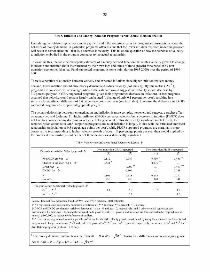
Box 5. Inflation and Money Demand: Program versus Actual Remonetization

Underlying the relationship between money growth and inflation projected in the program are assumptions about the behavior of money demand. In particular, programs often assume that the lower inflation expected under the program will result in remonetization—that is, a decrease in velocity. This raises the question of how the response of velocity to inflation embodied in the program compares to the actual relationship. To examine this, the table below reports estimates of a money demand function that relates velocity growth to change in income and inflation (both instrumented by their own lags and terms of trade growth) for a panel of 59 non-transition economies (that had Fund-supported programs at some point during 1995-2000) over the period of 1994-2003. There is a positive relationship between velocity and expected inflation: since higher inflation reduces money demand, lower inflation should raise money demand and reduce velocity (column (1)). By this metric ( Bv∆ ), programs are conservative: on average, whereas the estimate would suggest that velocity should decrease by 3½ percent per year in GRA-supported programs (given their programmed decrease in inflation), in fact programs assumed that velocity would remain largely unchanged (a change of only 0.1 percent per year), resulting in a statistically significant difference of 3.4 percentage points per year (see text table). Likewise, the difference in PRGF-supported program was 1.7 percentage points per year. The actual relationship between remonetization and inflation is more complex however, and suggests a ratchet effect on money demand (column (2)): higher inflation (DPOS) increases velocity, but a decrease in inflation (DNEG) does not lead to a corresponding decrease in velocity. Taking account of this statistically significant ratchet effect, the remonetization assumed in GRA-supported programs due to disinflation is largely in line with the estimated empirical relationship (a deviation of 0.3 percentage points per year), while PRGF-supported programs are marginally more conservative (corresponding to higher velocity growth of about 1½ percentage points per year than would implied by the empirical relationship)—but neither of these deviations is statistically significant.

(1) (2) (1) (2)

Real GDP growth 2/ 0.112 -0.047 0.399 * 0.451 **

Change in inflation (∆π ) 2/ 0.531 * … 0.335 *** … DPOS*∆π 2/ … 0.909 ** … 0.433 ***

DNEG*∆π 2/ … -0.106 … 0.169

R2 0.106 0.118 0.213 0.217No. obs. 250 250 340 340

Program versus benchmark velocity growth 3/∆vP - ∆vB 3.4 2.2 1.7 1.1∆vP- - ∆vB- … 0.3 … 1.5

Source: International Monetary Fund, MONA and WEO database; staff estimates1/ All regressions include country dummies; significant at: *** 1percent, ** 5 percent, * 10 percent.

3/ ∆vP refers to programmed velocity growth; ∆vB is the benchmark velocity growth constructed by using the estimated coefficients and programmed change in inflation (∆πP) and real GDP growth(∆yP); ∆vP- and ∆vB- represent, respectively, the values of ∆vP and ∆vB for disinflation programs (with ∆πP < 0) only.

Table. Velocity and Inflation: Panel Regression Results 1/

Dependent variable: Velocity growth 2/ Non-transition GRA-supported Non-transition PRGF-supported

2/ DPOS and DNEG are dummy variables that equal 1 if ∆π >0 and ∆π < 0, respectively, and 0 otherwise; all regressors are instrumented by their own 3 lags and the terms of trade growth; real GDP growth and inflation are transformed to be mapped into an interval (-100,100) to reduce the influence of outliers.

_______________________ 1 The money demand function takes the form em p yα βπ− = − . Taking first differences and re-arranging gives:

( 1) ev m y yπ α β π∆ ≡ ∆ − − ∆ = − ∆ − ∆

- 29 -

from higher growth raising revenues and improving the fiscal balance), these findings suggest that programs project too large a negative impact on growth and too small a positive impact on the current account balance of a given fiscal tightening.45

C. Medium-Term Growth and Debt Sustainability

38. Recent debt crises in emerging market economies as well as the need for debt relief for low-income countries have underscored the importance of accurate debt sustainability analyses. As discussed above, the Fund’s debt sustainability template is intended to bring greater discipline to such projections. Building on results for errors in projecting medium-term growth and the current account balance, this section considers the sources of errors in projecting external debt ratios, while noting that the sample covered (1995-2000) precedes the introduction of standardized debt sustainability templates.

Medium-Term Growth

39. With the exception of the capital account crises, the medium-term growth projection error averaged over the three years following program approval is as large as, or larger than, the error in the year of program approval (Table 4). Among both GRA- (excluding transition economies and capital account crises) and PRGF-supported programs the average errors are statistically significant, raising questions about the accuracy of these medium-term growth projections.

40. In fact, with the exception of the industrialized countries, preliminary results suggest that projections from a cross-country growth model could outperform medium-term projections contained in staff reports (Box 6). Medium-term growth projections could be enhanced in a number of ways. One possibility would be to generate growth projections centrally using a cross-country growth model.46 However, this may be too mechanical and would need to be informed by additional information available to the country authorities and desk economists. A variant of this approach would be to estimate the cross-country model, but use its projections as a reference point and “reality check” for the projections prepared by national authorities and Fund country teams. Significant deviations from the projections

45 One explanation may be that the economy is assumed to be more closed than it is in reality, leading to the over estimation of the implicit Keynesian multiplier. Evidence presented in Macroeconomic and Structural Polices in Fund-Supported Programs using instrumental variable estimation (i.e., controlling for endogeneity), however, also finds a positive relationship between the fiscal balance and growth among Fund-supported programs.

46 The models could also be estimated for different types of countries to capture, for example, region-specific or economic structure-specific aspects that may have implications for growth.

- 30 -

Table 4: Medium-Term Program Projection Errors 1/

Number Average period t+1:t+3obs. Mean RMSE

error

Real GDP Growth

PRGF-supported programs 56 -1.3 *** 2.8GRA-supported programs

Transition 2/ 27 -0.5 2.9 Non-transition 2/ 35 -2.4 *** 4.3 CACs 3/ 7 -0.4 2.3


PRGF-supported programs 48 -2.2 *** 4.1GRA-supported programs

Transition 2/ 24 -0.8 2.6 Non-transition 2/ 28 1.6 *** 3.2 CACs 3/ … … …


* = significant at 10% level, ** = significant at 5% level, and*** = significant at 1% level.

1/ Data transformed so that it maps into the interval (-100, 100).Errors defined as actuals minus projections. Table constructedusing a dataset for countries with available information for year t,t+1, t+2, and t+3.2/ Excludes capital account crises.3/ CAC stands for capital account crises.

- 31 -

Box 6. Medium-Term Growth Projections Using Cross-Country Growth Models

Fund growth projections tend to be overly optimistic as documented in a number of reports and forums; for example, the PRSP/PRGF reviews and PRSP progress report, the IEO’s reports on prolonged users of Fund resources and on fiscal adjustment in Fund-supported programs, and reports on IMF projections prepared outside the institution (such as the US General Accounting Office, 2003, and the Heritage Foundation, 1999). As discussed elsewhere in this paper, the 1- and 3-year ahead projection errors average about 1¼ percent per year. Similar biases apply to 5-year ahead projections

Can these projections be improved?

Improving growth projections is not an easy task, in part because they are conditional on the implementation of policies and on the absence of shocks. Still, a number of analytical methods are available. One method is reduced form growth equations. While these equations have many recognized weaknesses (e.g., unstable coefficient estimates and lack of a theoretical foundation), they also have advantages, in particular the drawing together of cross-country information. Although these equations are ill-suited for short-term projections, working backwards they serve to cap over-optimistic tendencies. In addition, they offer a benchmark against which to argue about a country’s growth potential.

To this end, a cross-country growth equation is estimated for the 5-year periods between 1981 and 1995 and one out-of-sample projection is carried out for 1996-2000. The projections are based on historical trends for the right hand variables in the equation and on projections for the two macro indicators in the equation (inflation and fiscal balance). The latter serves as control for the macro (but not the structural) aspects on which country projections are based.

What are the results?

The results, which focus on the projection accuracy (Theil U-statistic: the ratio of the root mean square errors of the model projections relative to those derived by country desks, with a value less than one implying that the model is more accurate), suggest that the model outperforms projections in developing countries, but performs very poorly among high-income countries. The differences in the model and projections are, on aggregate, statistically significant. These results must be qualified, however, by the fact that the results apply to only one out-of-sample forecast period (1996-2000).

Medium-Term Growth Projections (1996-2000)

Value Number ofcountries

Error in country projections 1.37 109Average error in growth equation projections 0.36 109

Total Theil U 0.85 109 High-income 1.22 14 Upper middle-income 0.99 20 Lower middle-income 0.91 32 Low-income 0.77 43

- 32 -

implied by the cross-country growth model would warrant closer scrutiny. This could include an analysis of the explanatory variables expected to generate the faster growth, a more detailed understanding of the country’s own past growth performance vis-à-vis the model, or a comparison of the model’s projections for a particular country relative to those of neighboring countries facing similar economic challenges. Even a discussion of why the cross-country growth model may be performing poorly for a given country could be revealing and may help identify specific growth bottlenecks facing a country.

Debt Sustainability

41. Both errors in projecting output growth and in projecting the current account balance feed into projections errors for the external debt ratio.47 Regarding the current account balance, on average during a three-year period, the balance is higher (or the deficit is smaller) by 1½ percent of GDP in non-transition GRA-supported programs. PRGF-supported programs continue their under-adjustment (relative to program projections), on average by about 2¼ percent of GDP during a three-year period (Table 4). Since external debt is normally denominated in foreign currency, debt-projection errors are affected by unanticipated real exchange rate movements.

42. To quantify the importance of these three sources of errors, Table 5 decomposes the difference between the actual48 and programmed debt ratio into the part attributable to

47 As discussed in Lessons from the Crisis in Argentina (SM/03/345), for example, optimistic growth projections during the early- and mid-1990s, partly based on reforms undertaken earlier in the decade, resulted in overly sanguine assessments of public and external debt sustainability.

48 To derive a consistent external debt series, the current account deficit (net of FDI) is accumulated starting from the level of external debt in the year preceding the program. The only differences between the level of external debt thus implied and the actual level of external debt should arise from changes in coverage or movements of cross-exchange rates (relative to the U.S. dollar) of the currencies in which countries might be borrowing (generally, Yen or Euro). Macroeconomic and Structural Policies in Fund-supported programs reports similar decomposition for public debt dynamics.

- 33 -

Tabl

e 5:

Dec

ompo

sitio

n of

Deb

t to

GD

P Pr

ojec

tion

Erro

rs (a

ccum

ulat

ed e

rror

s at e

nd p

erio

d; in

per

cent

of G

DP)

Num

ber

Act

ual

Erro

r as o

f end

of p

erio

d t

Erro

r as o

f end

of p

erio

d t+

1Er

ror a

s of e

nd o

f per

iod

t+2

Proj

.A

ctua

lob

s.de

bt in

Gro

wth

Exch

ange

Adj

ustm

ent

Tota

lG

row

thEx

chan

geA

djus

tmen

tTo

tal

Gro

wth

Exch

ange

Adj

ustm

ent

Tota

lde

bt in

debt

int-1

effe

ctra

teef

fect

effe

ctef

fect

rate

effe

ctef

fect

effe

ctra

teef

fect

effe

ctt+

2 1

/t+

2 2

/ef

fect

effe

ctef

fect

PRG

F-su

ppor

ted

prog

ram

s55

118.

00.

8-0

.41.

92.

43.

03.

23.

910

.24.

37.

85.

717

.810

5.3

123.

2

GRA

-sup

porte

d pr

ogra

ms

Tra

nsiti

on

3/21

41.8

0.2

0.3

-0.1

0.4

0.6

1.2

0.9

2.7

0.7

2.8

2.1

5.6

30.3

36.0

Non

-tran

sitio

n 3

/31

53.7

0.7

1.1

-2.0

-0.2

1.2

-1.4

-3.8

-4.0

2.6

-0.5

-3.2

-1.0

47.1

46.0

CA

Cs

4/

550

.65.

433

.1-7

.930

.77.

729

.3-1

5.3

21.7

7.5

26.1

-20.

513

.152

.865

.9

Sour

ce: M

ON

A a

nd W

EO d

atab

ases

, and

staf

f est

imat

es.

1/ D

eriv

ed b

y ad

ding

the

proj

ecte

d cu

rren

t acc

ount

bal

ance

to th

e t-1

act

ual d

ebt s

tock

afte

r adj

ustin

g fo

r FD

I flo

ws.

Lack

of F

DI d

ata

in th

e M

ON

A d

atab

ase

resu

lts in

the

use

of a

ctua

l FD

I dat

a.2/

Der

ived

by

addi

ng th

e ac

tual

cur

rent

acc

ount

bal

ance

to th

e t-1

act

ual d

ebt s

tock

afte

r adj

ustin

g fo

r act

ual F

DI f

low

s. M

ay d

iffer

from

act

ual W

EO d

ata

on d

ebt d

ue to

cha

nges

in c

over

age

and

chan

ges i

n cr

oss-

exch

ange

.rate

s of t

he c

urre

ncie

s in

whi

ch a

cou

ntry

's de

bt is

den

omin

ated

.3/

Exc

lude

s cap

ital a

ccou

nt c

rises

.4/

CA

C st

ands

for c

apita

l acc

ount

cris

es.

- 34 -

current account deficits, real exchange rates, or real GDP growth.49 In PRGF-supported programs, the average initial debt to GDP ratio was 118 percent of GDP and was projected to decline to 105 percent in three years. However, the actual ratio rose to 123 percent of GDP over the three-year period. The divergence over a three-year period between projected and actual face-value of external debt thus amounted to almost 18 percent of GDP.50 Lower-than-projected growth contributed 4¼ percentage points of GDP to this error, larger real exchange rate depreciation contributed a further 8 percentage points, while larger current account deficits than programmed accounted for another 5¾ percentage points.

43. Among GRA-supported programs, the initial level of external debt averaged 49 percent of GDP and was projected to decline to 41 percent, but in fact declined by less to 44 percent of GDP. The decomposition depends upon the type of country. For transition economies, which saw a significant increase in growth during this period, the projection error was larger (equivalent to 6 percent of GDP; Table 5). The error in projecting growth contributes roughly ¾ percentage points to the debt projection error, larger real exchange rate movements account for a further 3 percentage points, and less current account adjustment than anticipated adds another 2 percentage points of GDP. In non-transition GRA programs (excluding capital account crises), the projection error was negligible (1 percentage point of GDP). Lower growth accounted for 2½ percentage points of the error—which is more than 49 Define 10

(1 )a k a

t i tt k iy g y+ −+ =

= +∏ as the actual level of GDP at a constant U.S. dollar value

of the GDP deflator, where 1aty − is the U.S. dollar value of nominal GDP in year t-1, and g is

the real GDP growth rate. Likewise, define 10(1 )

p k p at i tt k i

y g y+ −+ == +∏ as the projected level of

GDP at a constant U.S. dollar value of the GDP deflator. Then the projection error in the debt ratio at any horizon k can be written:

a p a p p p p p p pt k t k t k t k t k t k t k t k t k t ka p a a a a p p a pt k t k t k t k t k t kt k t k t k t k

deficit real exch rate real GDP growth

d d d d d d d d d dy y y y y yy y y y

+ + + + + + + + + +

+ + + + + ++ + + +

− = − + − − − + − 1442443 1444442444443 1442443

,

where the first term represents the effects of larger than expected deficits, the second term is the effect of the real exchange rate (i.e., the U.S. dollar value of the GDP deflator) depreciation, and the third term is the effect of lower real GDP growth. This accounting decomposition does not identify the underlying shocks, driving these deviations from the projections, such as exogenous terms of trade shocks, unpredictable disbursements of foreign aid, or policy slippages.

50 The increase in the net present value (NPV) of debt will be smaller since the current account adjustment error (which contributes 5.7 percent of GDP to the face-value projection error) will affect the NPV by (1 )GE CAD− , where GE is the grant element (equal to the ratio of the NPV to face value) and CAD is the current account deficit.

- 35 -

offset by greater external adjustment than the program anticipated. In capital account crises the projection error was largest (13 percentage points of GDP). Lower growth and greater real exchange rate depreciation together accounted for the debt ratio being almost 30 percentage points of GDP higher than projected, but over half this increase was offset by greater external adjustment than envisaged and less borrowing.

IV. CONCLUSIONS

44. In recent years, the circumstances under which members seek Fund support have evolved considerably, raising the question of whether the process of policy formulation and program design remains appropriate and whether analytical tools remain relevant.

45. While no single model or analytical framework is universally applicable, policy formulation relies on a variety of models and techniques and employs economic judgment. A key feature of this general approach is its flexibility and adaptability, with program reviews providing an opportunity to reassess policies. In this regard, financial programming provides a convenient approach to tie together projections for individual sectors while ensuring an internally consistent analysis. It also serves as a standardized ex post monitoring tool.

46. Such adaptability of policies is especially important in capital account crises where unanticipated capital flows may have pervasive macroeconomic consequences. As stressed in the recent theoretical literature, such capital flows can interact with balance sheet exposures, altering not only the magnitude but potentially even the sign of policy multipliers. Balance sheet approaches can shed some light on the possible magnitudes and effects of capital flows, but cannot provide precise predictions, and the data requirements are often formidable.

47. At short horizons relevant for setting macroeconomic policies and program targets, growth projections are not biased and the errors are relatively small—excluding capital account crises. Over longer horizons, however, programs systematically over-estimate growth, especially in low-income countries. Inflation is under-estimated both in the year of program approval but also in following years as programmed disinflation targets become more ambitious. Current account projections also exhibit some bias, albeit in opposite directions in GRA- and PRGF-supported programs.51 In GRA-supported programs, the current account balance improves by more than expected reflecting unanticipated capital outflows. In PRGF-supported programs, by contrast, current account adjustment fall short of expectations and foreign borrowing is higher than envisaged. These results have implications for the accuracy of debt sustainability assessments.

48. Greater understanding of what drives growth is critical to reduce the systematic bias in growth projections. While there is a substantial empirical literature on factors that could contribute to better growth performance—including macroeconomic stability and certain characteristics of institutions—analytical tools are generally lacking, and such tools as do 51 See also Fund-supported Programs: Objectives and Outcomes.

- 36 -

exist are not always fully used. Cross-country growth regressions can help identify some of the structural areas in which a country lags relative to comparator countries and thus might benefit from reforms, and might serve to discipline medium-term growth projections. At the same time, it is important not to over-estimate the growth benefits of specific structural measures—in particular effects that pertain to short-run growth should be distinguished from those that raise the country’s long-term growth potential.

49. Finally, the diversity of country experiences makes it difficult to formulate strong tests of whether programmed relationships between policies and targets have, at least on average, been correct. With this caveat in mind, it is noteworthy that programs on average project the behavior of the money multiplier as well as the relationship between broad money growth and inflation, and the relationship between government expenditure and output growth. However, programs underestimate the impact on the current account balance of an improvement in the fiscal balance, as well as the positive association between fiscal adjustment and output growth—implicitly assuming that the economy is more closed than it is in reality.

50. These findings suggest a number of priorities for future work. First, though the current approach of drawing on a variety of models and methods for short-term projections works reasonably well (in that biases in projections, except in regard to the capital account crises, are small), there remains scope for improvement—including through improved statistical data to provide a sounder basis for making projections. Second, both in low- and in middle-income countries, medium-term growth projections—necessary, inter alia, for debt sustainability analysis—need to be improved and disciplined. Third, since in capital account crises the behavioral response of the economy depends on private capital flows, gaining a better understanding of the determinants of such flows could contribute significantly to better program design. Fourth, relatedly, recent theoretical models suggest that balance sheet effects can potentially alter the magnitude and sign of policy multipliers; further development and wider application of the balance sheet approach could help resolve some of the ambiguities that arise during such crises. Finally, national authorities and Fund country teams working collaboratively might explore more systematically the scope for using small econometric models, sharing experiences, and disseminating information on best practices, thus contributing to better designed—and better owned—Fund-supported programs. In a related-fashion, a more candid discussion of deviations between program targets and outcomes during program reviews could serve to provide better guidance for the design (and revision) of Fund-supported programs.

- 37 -

References

Agenor, P., and P. Montiel, 1999, “Development Macroeconomics,” Princeton University Press.

Aghion P., and A. Banerjee, 2001, “Currency Crises and Monetary Policy with Credit Constraints,” European Economic Review, Vol. 45, No.7, pp. 1121-50.

Allen, M., C. Rosenberg, C. Keller, B. Setser, and N. Roubini, 2002, “A Balance Sheet Approach to Financial Crisis,” IMF Working Paper No. 02/210.

Baqir, R., R. Ramcharan, and R. Sahay, 2004, “IMF Program Design and Growth. Is Over-Optimism Deliberate? Is it Defensible,” mimeo, International Monetary Fund.

Batista, C. and J. Zalduendo, 2004, “Can IMF Medium-Term Growth Projections Be Improved?,” IMF Working Paper No. 04/203.

Boughton, J. 2001, “Different Strokes? Common and Uncommon Responses to Financial Crises,” IMF Working paper No. 01/12.

Borensztein, E., and A. Ghosh, 1989, “Foreign Borrowing and Export Promotion Policies,” IMF Staff Papers, 36.

Bubula A., and I. Otker-Robe, 2002, “The Evolution of Exchange Rate Regimes since 1990: Evidence from De Facto Policies,” IMF Working Paper 02/155.

__________, 2003, “Are Pegged and Intermediate Exchange Regimes More Crisis Prone?,” IMF Working Paper No. 03/223.

Cespedes, L., R. Chang, and A. Velasco, 2003, “IS-LM-BP in the Pampas,” IMF Staff Papers, Vol. 50, pp. 143-64.

Cohen, D., and J. Sachs, 1986, “Growth and External Debt under Risk of Repudiation,” European Economic Review, 30, pp. 529-50.

Coorey, S., M. Mecagni, and E. Offerdal, 1996, “Disinflation in Transition Economies: The Role of Relative Price Adjustment,” IMF Working Paper No. 96/138.

Dornbusch, R., 1990, “Policies to Move from Stabilization to Growth,” CEPR Paper No.456.

Duttagupta, R., G. Fernandez, and C. Karacadag, 2004, “From Fixed to Float: Operational Aspects of Moving Towards Exchange Rate Flexibility,” IMF Working Paper No. 04/126.

Easterly, W., 2002, “An identity Crisis? Testing IMF Financial Programming,” Center for Global Development Working Paper No.9.

Edwards, S., 1989, “The International Monetary Fund and the Developing Countries: A Critical Evaluation,” NBER Paper No.2909.

__________, 1989, “What does the International Monetary Fund Really Do? Reply to Goldstein,” Carnegie-Rochester Conference Series on Public Policy, 31, 77-82.

- 38 -

Eichengreen, B. et al., 1998, Exit Strategies: Policy Options for Countries Seeking Greater Exchange Rate Flexibility, IMF Occasional Paper No. 168.

Eichengreen, B., and R. Hausmann, 1999, “Exchange Rates and Financial Fragility,” NBER Paper No. 7418.

Froot, K., and R. Thaler, 1990, “Anomalies: Foreign Exchange,” Journal of Economic Perspectives, Summer, pp. 179-92.

Funke, Norbert, 1993, “Timing and Sequencing of Reforms: Competing Views and the Role of Credibility,” Kyklos, Vol. 46, pp. 337-362.

Furman. J., and J.E. Stiglitz, 1998, “Economic Crises: Evidence and Insights from East Asia, Brookings Papers on Economic Activity 2 (Washington DC: Brookings Institution)

Gapen, M., G. Dale, C. Lim, and Y. Xiao, 2004, “The Contingent Claims Approach to Corporate Vulnerability Analysis: Estimating Default Risk and Economy-wide Risk Transfer,” IMF Working Paper No. 04/121.

Goldfeld, S., and D. Sichel, 1990, “The Demand for Money,” in Friedman, B. and Hahn, F. H. (Eds.), Handbook of Monetary Economics, Elsevier, Amsterdam.

Ghosh, A., 1997, “The Output-Inflation Nexus in Ukraine: Is there a Trade-off?,” IMF Working Paper No. 96/46.

Ghosh, A., and S. Phillips, 1998, “Inflation, Disinflation, and Growth,” IMF Working Paper No. 98/68.

Heisenberg, W., 1927, “Über den Anschaulichen Inhalt der Quantentheoretischen Kinematik und Mechanik,” Zeitschrift für Physik, Vol. 43, 172-198. Translated into English by John Archibald Wheeler and Hubert Zurek, in Quantum Theory and Measurement, Wheeler and Zurek, eds. (Princeton: Princeton Univ. Press, 1983), pp. 62-84.

Issing, O., 1992, “Theoretical and Empirical Foundations of the Deutsche Bundesbank's Monetary Targeting,” Intereconomics, Nov/Dec 1992. Vol. 27, No. 6.

________, 1997, Monetary Targeting in Germany: The Stability of Monetary Policy and of the Monetary System, Journal of Monetary Economics, Vo. 39(1).

International Monetary Fund, 1997, “The ESAF at Ten Years: Economic Adjustment and Reform in Low-Income Countries,” (Washington: IMF, December).

Jager, H., 1994, “Comment on Manuel Guitian: The Role of Monetary Policy in IMF Programs,” in A Framework for Monetary Stability, Kluwer Academic Publishers.

Jeanne, O., and J. Zettelmeyer, 2002, “Original Sin, Balance Sheet Crises and the Roles of International Lending,” IMF Working Paper No. 02/234.

Joshi, B., and A. Ghosh, 2003, “How Good (Or Bad) are Fund Projections?,” mimeo, International Monetary Fund.

Kaufmann, D., A. Kraay, and P. Zoido-Lobatón, 1999, “Governance Matters,” Washington, DC, The World Bank, Policy Research Working Paper 2196.

- 39 -

Khan, M., and P. Montiel, 1989, “Growth-Oriented Adjustment Programs: A Conceptual Framework,” IMF Staff Papers, Vol. 36.

Killick, T., 1995, “IMF Programs in Developing Countries. Design and Impact,” Routledge London and New York.

Lown, C., S. Peristiani, and K. Robinson, 1999, “What Was Behind the M2 Breakdown?,” Financial Industry Working Paper No. 99-2, Federal Reserve Bank of Dallas.

Lucas, R., 1976, “Econometric Policy Evaluation: A Critique,” Carnegie-Rochester Conference Series on Public Policy, 1.

MacDonald, R., and M. Taylor, 1992, “Exchange Rate Economics: A Survey,” IMF Staff Papers, International Monetary Fund, Vol. 39(1).

Mauro, Paolo, 1995, “Corruption and Growth,” The Quarterly Journal of Economics, 110 (3): pp. 681-712.

Michaely, Michael, D. Papageorgiou, and A. Choksi, 1990, “Liberalizing Foreign Trade in Developing Countries: The Lessons of Experience,” Washington, DC, The World Bank.

Montiel, P., 2003, “Tight Money in a Post-Crisis Defense of the Exchange Rate: What Have We Learned?,” The World Bank Research Observer, vol. 18, no.1 (Spring), pp.1-23.

Morgenstern, O., 1950, On the Accuracy of Economic Observations,” (Princeton NJ: Princeton University Press).

Mussa, M., and M. Savastano, 1999, “The IMF Approach to Economic Stabilization,” IMF WP/99/104.

Musso, A., and S. Phillips, 2001, “Comparing Projections and Outcomes of IMF-Supported Programs,” IMF Working Paper No. 01/45.

Nsouli, Saleh, Mournir Rached, and Norbert Funke, 2002, “The Speed of Adjustment and the Sequencing of Economic Reforms: Issues and Guidelines for Policymakers,” IMF Working Paper, International Monetary Fund, WP/02/132.

Polak, J. J., 1957, “Monetary Analysis of Income Formation and Payments Problems,” IMF Staff Papers, Vol. 5, November.

Ramcharan, R., 2004, “How Well-Designed Are IMF Programs?” mimeo, International Monetary Fund.

Reinhart, C., and K. Rogoff, 2004, “The Modern History of Exchange Rate Arrangements: A Reinterpretation,” Quarterly Journal of Economics, 119, 1, pp.1-48.

Robichek, E.W., 1967, “Financial Programming Exercises of the International Monetary Fund in Latin America,” mimeo, Rio de Janeiro.

Robichek, E.W., 1971, “Financial Programming: Stand-by Arrangements and Stabilization Programs,” mimeo, (Washington: International Monetary Fund).

- 40 -

Rogoff, K. et al., 2004, Evolution and Performance of Exchange Rate Regimes, IMF Occasional Paper No. 229.

Sarel, M., 1996, “Nonlinear Effects of Inflation on Economic Growth,” IMF Staff Papers, International Monetary Fund, Vol. 43(1).

Senhadji, A., and M. Khan, 2000, “Threshold Effects in the Relationship Between Inflation and Growth,” IMF Working Paper No. 00/110.

Taylor, L, 1988, “Varieties of Stabilization Experience,” Clarendon Press, Oxford.

Zalduendo, J., 2004, “The Design of Macroeconomic Policies and Structural Reforms,” mimeo, International Monetary Fund.

- 41 - APPENDIX I

The Financial Programming Model

1. “Financial programming” has been used in different contexts and with different meanings. At one extreme, financial programming is an economic model linking the financing of the fiscal deficit to the behavior of foreign exchange reserves (or, under a floating regime, exchange market pressures). This model, first articulated in a series of papers by Polak (1957) and Robichek (1967, 1971), was developed in a world of fixed (but adjustable) parities, generally limited recourse to domestic bond financing by governments, and little or no mobility of private capital (IMF (1987)). In order to deliver this predicted relationship, the model requires a number of simplifying behavioral assumptions, including exogeneity of growth, no bond financing (at the margin) of the fiscal deficit, and stability of money demand. Even when these assumptions are violated, however, the identities underlying the financial programming framework must hold. At the very least, therefore, the framework provides a convenient consistency check on macroeconomic projections underlying program design. In practice, financial programming is often used as a general approach—helping to inform projections of individual sectors (external, monetary, fiscal) without pinning down precisely every parameter of the program—but, depending upon country circumstances, as more than a mere set of identities that must hold for any set of consistent projections.

2. This appendix lays out the basic financial programming model, discusses some of its advantages and weaknesses as well as the circumstances in which the financial programming as a general approach is likely to be useful.

Basic formulation of financial programming

3. Base money ( M ) consists of domestic credit to the government ( GDC ), the private sector ( pDC ), or international reserves (R )52:

G pM DC DC e R∆ ≡ ∆ + ∆ + ∆ (1)

e is a fixed or given exchange rate. The government finances its deficit by borrowing from the central bank, the domestic bond market GB or (in foreign currency) from the international capital markets *

GB :

*G G GDef DC B e B= ∆ + ∆ + ∆ (2)

Real output growth is projected, y y∆ = ∆ , the inflation target is given, π π= , and velocity, v, is predictable, therefore money demand is predictable: 52 The model can be applied to the central bank’s balance sheet (as done here) or to the banking system aggregates under the assumption of a stable money multiplier.

- 42 - APPENDIX I

( )M M M y vπ∆ = ∆ = ∆ + + ∆ (3) Substituting (1) and (3) into (2) yields:

* ( )G G PDef e B B M DC e R= ∆ + ∆ + ∆ − ∆ − ∆ (4)

Assuming that the government has, at the margin, no recourse to bond financing *0, 0G GB B∆ = ∆ = , a reserves target, R R∆ = ∆ at a given exchange rate, e , and that there is

a required minimum expansion of credit to the private sector, ppDC DC∆ = ∆ , gives a limit on the financeable budget deficit:

( )pDef M DC e R= ∆ − ∆ − ∆ (5)

Modeling advantage of financial programming

4. As a means of modeling the balance of payments, financial programming offers a number of advantages. It provides a direct link between policies (the fiscal deficit, monetary policy) and the reserves target while requiring only central bank (or banking system) balance sheet data, which should be readily available for both program projections and monitoring. Another advantage is that by exploiting Walras’ Law and the assumed stability of money demand it obviates the need to model private capital flows, which is an important advantage inasmuch as existing empirical models of capital flows—based, for instance, on interest parity conditions—tend to perform very poorly.

5. To see the last point, the balance of payments identity can be rewritten: * *( ) ( ) ( , ) ( )p p G g p GS I S I CA y e e B e B R− + − = = − ∆ − ∆ − ∆ (6)

which states that, at a given level of economic activity and exchange rate, the current account deficit must be financed by net borrowing by the private sector, *

pB∆ , or borrowing by the

public sector (net of its accumulation of reserves), *GB R∆ − ∆ . Using the identity that private

saving must take the form of acquiring government bonds, foreign assets, base money (net of credit extended to the private sector) or domestic physical assets:

ppGpp IBeBDCMS +∆−∆+∆−∆= *)( (7)

and substituting (7) into (6) gives: * * *( ) ( )p G p p GM DC B e B Def e B e B R∆ − ∆ + ∆ − ∆ − = − ∆ − ∆ − ∆ (8)

so the term representing private capital flows, *pe B∆ , cancels on both sides of the equation,

yielding the familiar financial programming relationship between the fiscal deficit and the accumulation of reserves as shown in (4).

- 43 - APPENDIX I

Criticism of financial programming

6. The very simplicity of the financial programming framework, however, is the basis of much of its criticism. Common criticisms center on the theoretical limits to the approach, and on the realism of its underlying assumptions. It is often argued, for instance, that governments typically have at least some scope for bond financing, that real growth is not sufficiently endogenous with respect to the macroeconomic policies (Edwards (1989), Killick (1995), and Taylor (1988)), and that money demand is unlikely to be predictable. The model can, in part, accommodate these criticisms. For example, specific projections of the government’s ability to borrow internationally or in the domestic bond market are readily accommodated within the framework—although significant reliance on nonbank financing requires a shift in focus to the overall fiscal deficit from controlling the size of the bank financed fiscal deficit. Likewise, by postulating a link between the provision of credit to the private sector and economic activity, it is possible to endogenize the behavior of output growth, though the framework is not well suited to handling Keynesian effects and is clearly not intended as a model of long-term growth.53

7. The charge that money demand may be unpredictable is potentially more telling, since predictable money demand is the cornerstone of the financial programming approach.54 Ultimately, however, whether money demand is predictable is an empirical question that needs to be viewed against uncertainties in other economic relationships. Import and export demand functions, for instance, may also be difficult to predict, so that alternative approaches to modeling the balance of payments, and the link to macroeconomic policies, may be equally—or more—unreliable.

8. Money demand is likely to be highly unpredictable when private capital flows are large and volatile. As noted above, financial programming dispenses with the need to model private capital flows, but this modeling advantage may be somewhat illusory if volatility of

53 Ghosh (1997) develops a simple empirical model in which output growth depends upon real credit to the private sector, and applies it to the effects of credit expansion (to finance a fiscal deficit) on the dynamics of inflation, wages, the exchange rate, and output.

54 Empirical studies suggest that, at least in industrialized countries, traditional money demand functions began to break down in the late 1970s and 1980s. Notably, in the United States, a deterioration in the link between M2 and GDP over the 1980s led the Federal Reserve to drop M2 as a reliable indicator of monetary policy in 1993. Goldfeld and Sichel (1990) attributed the instability to deregulation and financial innovation and suggested that using broader monetary aggregates might yield more stable results. Indeed, in Germany, financial innovation played a less important role than in other countries contributing to its relatively stable money demand (Issing, 1992 and 1997). More recent studies incorporating financial innovation variables and better econometric tools have yielded somewhat more stable results (for example, see Lown, et al., 1999).

- 44 - APPENDIX I

private capital flows is manifested elsewhere in the economy. Of particular concern is a situation in which the “tail wags the dog”—that is, capital flows are largely autonomous and represent an independent influence on the balance of payments with the current account balance (and thus the exchange rate and economy activity) driven by capital flows. In this situation, projections of money demand are likely to be unreliable and financial programming as well as other approaches may be of limited ability for modeling the balance of payments and exchange market pressures. It is noteworthy in this respect that the volatility of reserve money velocity rose substantially in capital account crises whereas it fell during the program period in PRGF-supported countries (the trend in other GRA-supported is indeterminate); Table 1.55 Moreover, the link between fiscal balances and reserve accumulation—predicted by financial programming—is stronger among PRGF-supported countries (Table 2).

55 Ramcharan (2004) argues that volatility of velocity in ESAF/PRGF-supported programs is greater; this refers to the variance across programs rather than the time series volatility of a given country—which is more pertinent to whether the financial programming model should be applied. A separate issue concerns the difference between programmed and actual velocity, which is discussed in Macroeconomic and Structural Policies in Fund-supported Programs: Review of Experience.

σ(t-5,t-1) σ(t,t+3) σ(t-5,t-1) σ(t,t+3) σ(t-5,t-1) σ(t,t+3)Reserve money velocity Average 15.0 9.3 10.5 10.2 8.7 14.6 Median 12.2 7.5 8.9 9.1 8.5 12.5

1/ Velocity is defined as reserve money divided by nominal GDP; volatility is measured by standard deviation of velocity growth.

PRGF-supported GRA-supported Capital account crises

Table 1. Volatility of Reserve Money Velocity 1/(In percent per year)

Const. ∆GBAL 1/ R2 no. obs. Const. ∆GBAL 1/ R2 no. obs. ∆RES 1/ 1.351 ** -0.309 ** 0.121 41 0.929 * 0.412 * 0.135 23

∆(∆RES) 1/ -0.571 -0.440 ** 0.137 40 -0.263 0.360 0.055 221/ RES and GBAL refer to foreign reserves and general government balance in percent of GDP of the previous year, respectively; ∆ indicates a first difference; *: significant at 10%; **: significant at 5%; ***: significant at 1%.

Table 2. Change in Fiscal Balance, Reserve Accumulation and Change in Reserve Accumulation: Regression Results

Dependent Variable GRA-supported PRGF-supported

Policy Formulation, Analytical Frameworks, and Program ... · analytical tools and approaches to...

Documents

Transcript of Policy Formulation, Analytical Frameworks, and Program ... · analytical tools and approaches to...