Police Personnel - OJP
143
U.S. Department of Transportation National Highway I Traffic Safety Administration 0' LO Police Personnel Allocation Manual State-Wide Agencies User's Guide If you have issues viewing or accessing this file contact us at NCJRS.gov.
Transcript of Police Personnel - OJP

U.S. Department of Transportation
National Highway I Traffic Safety
Administration
~
0' ~ LO
Police Personnel Allocation Manual State-Wide Agencies
User's Guide
If you have issues viewing or accessing this file contact us at NCJRS.gov.

POLICE ALLOCATION MANUAL
USER'S GUIDE
Determination of the Number and Allocation of Personnel for
Police Traffic Services for State-Wide Agencies
- PAM Version 4.0-
July 1991
Prepared by
THE TRAFFiC INSTIlUTE Northwestern University
for
APR 2"f(f 1995
NATIONAL HIGHWAY TRAFFIC SAFETY ADMINISTRATION U. S. Department of Transportation
Contract No. DTNH22-88-C-05016
__ ~ __ ~ __ ~ ________________________ ---J
U.S. Department of JUstIce National Institute of JUstice
154016
This document has been reproduced exactly as received from the person or organization originating it. Points of view or opinions stated in this document are those of the authors and do not necessarily represent the official position or pol/cies of the National Institute of Justice.
Permission to reproduce this ~U material has been granted by • • Pub.L~C Ibmam U. S. Department of TransFOrtat~on
to the National Criminal Justice Reference Service (NCJRS).
Further reprodUction outside of the NCJRS system requires permission of the~ owner.
~------------ J

Version 4.0 - July 1991
FOREWORD
The Police Allocation Manual (PAM) and the Police Allocation Manual User's Guide were developed and field tested by The Traffic Institute of Northwestern University under a contract (No. DTNH22-88-C-05016) issued by the Office of Traffic Safety of the National Highway Traffic Safety Administration, U.S. Department of Transportation. principal Investigator and author for the study was Dr. William Stenzel. Dr. Stenzel was assisted by Mr. Roy Lucke who had prime responsibility for the design, implementation, and coordination of the field test program. The Contracting Officer's Technical Representative for the project was Mr. David Seiler (The Office of Traffic Safety).
The PAM project was initiated in June 1988 and Phase I was completed in February 1990. The Phase I field test was conducted during the summer and fall of 1989. Phase II of the project was completed in July 1991. Several versions or "editions" of the Manual were produced during the project. Version 1.0 was completed in March 1989. Version 2.0 was completed in June 1989 and was used for the Phase I field test. Version 3.0 was completed at the end Phase I (February 1990), Version 3.5 was submitt2d to NHTSA in January 1991, and Version 4.0 was completed in July 1991.
The project team wishes to thank the following state agencies which served as field test sites for the study. (The project liaison person for each agency is identified with an "*". Ranks and titles reflect those held during the Phase I field test.)
Arizona Department of Public Safety
Lt. Colonel Larry N. Thompson, Chief Arizona Highway Patrol Bureau
* captain Coy Johnston Arizona Highway Patrol Bureau
Trooper Jack Bell Arizona Highway Patrol Bureau
iii

version 4.0 - July 1991
California Highway Patrol
Colorado state Patrol
Florida Highway Patrol
Illinois state Police
commissioner M. J. Hannigan Department of California Highway
Patrol
* captain Gary Townsend Operational Planning section Department of California Highway
Patrol
Captain Robert Haworth operational Planning section Department of California Highway
Patrol
Mr. Alan J. Bailey Operational Planning Se~~ion Department of California Highway
Patrol
Colonel John N. Dempsey, Chief Colorado state Patrol
* Lt. Ralph Martin Colorado state Patrol
Lt. Michael Farnsworth Colorado state Patrol
Ms. Leslie Nelson Colorado state Patrol
Bobby R. Burkett, Director Florida Highway Patrol
* Mr. James M. Roddenberry Management Review Specialist Florida Highway Patrol
William O'Sullivan, Deputy Director Division of State Troopers
* Mr. James G. Milbr~ndt, Bureau Chief Management Information Bureau Illinois State Police
Mr. Charles Clark Management Information Bureau Illinois State Police
iv
____ ~J

!"
Massachusetts state police
Nebraska state Patrol
New York state Police
Version 4.0 - July 1991
William McCabe, Commissioner Massachusetts state Police
* Lt. Col. Thomas J. Kennedy Research and Development Massachusetts state Police
Corporal Alfred L. Lussier Research and Development Massachusetts state Police
Col. H. W. LeGrande, superintendent Nebraska state Patrol
Lt. Jerry Petersen Research and Planning Nebraska state Patrol
* Sgt. steve Evans Research and Planning Nebraska state Patrol
Ms. Diann Bauer Research and Planning Nebraska S'tate Patrol
Thomas A. constantine, superintendent New York State Police
* Lt. Colonel James McMahon Assist. Deputy Superintendent Planning and Research New York State Police
Mr. Leonard B. Clifford Planning and Research New York State Police
Completion of the Manual would not have been possible without the cooperation of the 46 state and provincial law enforcement agencies that provided information about their current staffing and deployment procedures to the project. A list of the 46 agencies is presented below:
Alabama Department of public safety
v
Alaska State Troopers

Version 4.0 - July 1991
Arizona Highway Patrol
California Highway Patrol,
connecticut state Police
Florida Highway Patrol
Idaho Department of Law Enforcement
Indiana state Police
Kansas Highway Patrol
Louisiana state Police
Massachusetts state Police
Minnesota state Patrol
Montana Highway Patrol
Nevada Highway Patrol
New Jersey state Police
North Carolina state Highway Patrol
Ohio state Highway Patrol
ontario Provincial Police
Pennsylvania state Police
Royal Canadian Mounted Police
Tennessee Hight·my Patrol
utah Highway Patrol
Virginia state Police
West Virginia state Patrol
Arkansas state Police
Colorado state Patrol
Delaware state Police
Georgia Department of Public Safety
Illinois state Police
Iowa state Patrol
Kentucky State Police
Maryland state Police
Michigan state Police
Missouri Highway Patrol
NebraS'll{a State Patrol
New Hampshire state Police
New York state Police
North Dakota Highway Patrol
Oklahoma Highway Patrol
Oregon State Police
Rhode Island state Police
South Dakota Highway Patrol
Texas Highway Patrol
Vermont State Police
Washington state Patrol
Wisconsin state Patrol
The project team also wishes to thank Messrs. Michael Buren and Alex Weiss of The Traffic Institute, Mr. sid Girling of the Ontario Provincial Police, and Mr. Richard Raub of the Illinois
vi

~------------------~----~---------------------'-~I
Version 4.0 - July 1991
state Police (ISP) all of whom reviewed initial drafts of the Manual and provided many valuable suggestions.
A special acknowledgment is extended to Mr. Raub of the ISP. Many of the ideas used in the Manual reflect concepts developed and documented by Mr. Raub and his colleagues in a series of ISP reports beginning in 1981. Mr. Raub's outstanding work into the identification and estimation of the major elements of staffing and allocation of state-wide police agency resources provided many of the basic components for the PAM model.
A special note of thanks is extended to Ms. Darry Ware whose diligence and persistence helped to insure that a steady stream of project materials were sent to the field test agencies in a timely manner.
vii
I
I
version 4.0 - July 1991
TABLE OF CONTENTS
FOREWORD • • • • • • • • .. • • • • • • • • • • • • II • ~ •• iii
TABLE OF CONTENTS . . . .. . . . . . . . . . . . . . . . . . SEC'IIION 1: INTRODUCTION • • • • 0 • •
Police Allocation Manual project o • • • e _ • • • • •
Police Allocation Manual Procedures • •
contents of the User1s Guide
How to Use the Guide . . . . . . . . . . . . - . . . .
SECTION 2: GENERAL IMPLEMENTATION STRATEGIES
Uses and Limitations of the Manual
Guidelines for First-Time PAM Users •
SECTION 3: DATA DEFINITION AND COLLECTION ISSUES
Data Collection Categories . . . . . . . Selecting Autonomous Patrol Areas (APAs)
state Agency Example #1 State Agency Example #2
Worksheet options and the Use of Performance
. . . . .
Standards _ . . . . .. ......... .
ix
1
1
1
2
3
3
3
5
6
6
8
9 9
10
Administrative Time per Trooper (Worksheet 2) 10 Table 1: Values Used for Selected PAM Input
Data Items, 1989 Phase I Field, Seven Agencies • • • • • • • • • • • • • 11
Self-Initiated Time per Trooper (Worksheet 4) 15 Patrol Availability (Worksheet 5) ........ 15
ix

-----------------
Version 4.0 - July 1991
Number of Staff and Command Personnel (Worksheet 8) .....•.•••• 15
strategies for Controlling the Data Collection Effort. 16
APA-Independent Data ••.••• ••• 16 APA-Dependent Data . .••• •.• 16 State Agency Example #1 • . • • . . . . . . • •• 17 State Agency Example #2 • • •• ••••••• 18 Table 2: APA category Characteristics r State
Agency #1 . . • . • • . . • . • • • •. 19 Table 3: APA Category Characteristics, state
Agency #2 . • . . • •• ••.• 19
Discussion of Individual Data Items •
Highway Types . • • • • . . • • . . • • • . • • • Immediate Response Percent .••••••.•• On-Duty Hours per Year per Trooper • • . • Patrol Coverage • • . . • . • . . • . • Patrol Interval • • . • • . Patrol Speed • . • • • • Response Speed . .•..•..••.••• • • Self-Initiated Time . .. •••. Service Time • . . • . . • • Shift Length . . . . . . • . . • • • . Special Assignment Personnel . • • . . • • • • • • Staff and Command Personnel Travel Time . . . . . . . . . . . . . . . . . . .
SECTION 4: RECOMMENDED DATA COLLECTION AND IMPLEMENTATION PROCEDURE . . • . • . . .• ..•.••.•.
20
20 21 21 22 22 22 23 24 24 25 26 26 26
27
step 1: Obtain Initial Staffing Level Estimates with Minimum Data Collection Effect . • . . • . . . 27
Step 2: Assess the Quality of the Input Data Items 27
Step 3: Investigate the Sensitivity of the Staffing Estimates to Changes in Individual Input Data Items . . . . . . . • . . . . . . . . •• 28
step 4: Improve Accuracy of Important Data Items 28
x

version 4.0 - July 1991
APPENDIX A: COMPREHENSIVE LIST OF PAM INPUT DATA . . ~-1
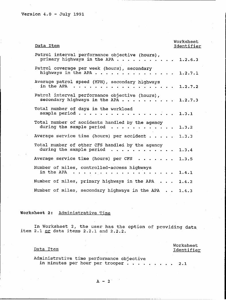
Worksheet 1: operations, Workload, and Highway Data A-I Worksheet 2: Administrative Time . • . • . . . • • A-2 Worksheet 3 : Reactive Time • . • . . • . • . • A-3 Worksheet Worksheet Worksheet
4: ::1 : 6:
Proactive Time - Self-Initiated . • • • . A-3 Proactive Time - Patrol • • • . . A-4 Average Daily Number of On-Duty
Troopers • • • • • • • • • • • • • A-4 Worksheet 7 : special Assignments and Field
supervision • . . • • • • .• .•• A-5 Worksheet 8: Total Staff Requirements . • • • A-6 Worksheet 9: Allocation of Patrol Personnel Among
Several APAs . • . . • . . • • A-6 Supplemental Worksheet: Patrol Availability -
Imnlediate Response • A-6
APPENDIX B: GLOSSARY AND WORKSHEET ABBREVIATIONS AND NOTATION . • . • • • • • • B-1
Glossary • • 0 • • • B-1
Worksheet Abbreviations and Notation B-11
APPENDIX C: EXAMPLE USING PAM WORKSHEETS 1-9 TO DETERMINE STAFFING REQUIREMENTS AND ALLOCATION • • • • • • C-1
Introduction
Observations
Example Worksheets
Worksheet 1:
Worksheet 2: Worksheet 3 : Worksheet 4: Worksheet 5: Worksheet 6:
Worksheet 7:
Worksheet 8: Workshee.t 9:
. . . . . . . . . . . . .
• • • • • • • • • It • • • • • •
Operations, Workload, and Highway • . . . . • . . . • .
Administrative Time • .. .•. Reactive Time . . . • . • . . • • . Proactive Time - Self-Initiated Proactive Time - Patrol • . . • • . Average Daily Number of On-Duty
Troopers • • • • • • . • • . • Special Assignments and Field
Supervision • . . . • • . • • Tot.:=tl Staff Requirements . . • • Allocation of Patrol Personnel
Among Several APAs • . . • . .
xi
C-1
C-1
C-6
C-6 C-9 C-11 C-13 C-16
C-25
C-28 C-35
C-39
_______ J

version 4.0 - July 1991
APPENDIX D: DERIVATION OF-MAJOR FORMULAS USED IN THE PAM MODEL • . • • . • • .• •••• • • . • D=l
D.1
D.2
D.3
D.4
D.5
Average Number of On-Duty Troopers (Nr ) Required Per Day Within the APA To Meet the Average Daily (Obligated Time) Workload, (3.3.3) .••••••••••
Average Number of On-Duty Troopers (Nppi) Required Per Day To Meet the Patrol Interval Performance Requirement Objective Within the APA, (5.1.2.5), (5.1.3.5), and (5.1.4.5) •••••.••••
Total Number of Troopers (N ri) Requir.ed Per Day within the APA ToPprovide Immediate Response To the Performance Objective Percentage of CFS, Accidents, and Self-Initiated Ac~ivities, (5.2.8) ...•..•
Average Number of On-Duty Troopers (Npao ) Required Within the APA To Meet the A~erage Travel Time Performance Objective for Area Patrol, (5.3.6.3) •..•••.••••••
Average Number of On-Duty Troopers (Np1P ) Required Within the APA To Meet the A~erage Travel Time Performance Objective for Line Patrol, (5.4.6) ..•••.•••••••
D.6 Average Total Number of On-Duty Troopers (N) Required Per Day for All Patrol Activities
D-2
D-4
D-9
D-16
D-20
Within the APA, One Trooper Per Unit, (6.1.5) D-23
D.7 Average Total Number of On-Duty Troopers (No) Required Per Day for All Patrol Activities Within the APA, Adjusted for One and Two Trooper units, (6.2.4) . . . • • . • . • . . D-27
D.8 Average Total Number of On-Duty Troopers (Not) and On-Duty Field Supervisors (Nos) Required Per Day for Patrol Activities Within the APA, Adjusted for the Presence of Field Supervisors and Special Assignment Personnel (7.2.4) and (7 • 3 . 1) ..................... 0--29
xii

Version 4.0 - July 1991
0.9 Determination of the Shift Relief Factor (SRF) for the Calculation of the Total Number of Troopers {Nt> and Field supervisors (Ns ) Required Within the APA, (8.3.1) and (8.3.2)
0.10 Allocation of Patrol Personnel Among Several APAs, Worksheet 9 • . • • • • • • • • . . •
xiii
0-34
0-37

version 4.0 - July 1991
SECTION 1: Introduction
Police Allocation Manual Project
The Police Allocation Manual User's Guide (herein after referred to as the Guide) is intended as a companion document to the Police Allocation Manual (PAM), Version 4.0, which can be used to determine the number and allocation of personnel for police traffic services fo~ state-wide agencies.
Both the Guide and the Police Allocation Manual (herein after referred to as the Manual) were developed by The Traffic Institute of Northwestern University under contract to the National Highway Traffic Safety Administration (NHTSA), U.S. Department of Transportation. A summary of project activities and products is contained in the Foreword and additional information about the project is contained in the Phase I and Phase II final reports submitted to NHTSA in February 1990 and March 1991 respectively.
Police Allocation Manual Procedures
The procedures described in the Manual for determining the number of staff are based on an analysis of trooper workload in terms of the amount of time required to complete various tasks. All trooper activities are assigned to four categories:
o Reactive: answering calls-for-service and responding to accidents;
o Proactive - Self-Initiated: traffic enforcement, field interrogations, motorist assists;
o Proactive - Patrol: patrol on uncommitted time; and
o Administrative: office time, vehicle maintenance, meal time, etc.
It is important to note that the definition for "patrol" used in the PAM model is narrower than that used by many law enforcement agencies. In PAM, the "Proactive-Patrol" workload category refers to uncommitted time only. Self-initiated activities which occur as a result of "proactive patrol" time are included in the "proactive sel f- ini tia ted " category. In other words, time spent
1
-I I I

version 4.0 - July 1991
looking for vi'.::>lators is "patrol" vlhile the time spent with violators is "seJLf-initiated."
The procedure~ used in the PAM model rely on historical data for the agency and user-supplied performance objectives. These data and objectives are used in nine worksheets in the Manual to guide the user through the process of determining how many troopers are needed for each of the categories identified above. For two of the categories, Reactive (Worksheet 3) and Proactive-Patrol (Worksheet 5), workload and performance obj ecti ves are used to derive the number of on-duty troopers required daily for each category. For the Administrative (Worksheet 2) and Proacti veSelf-Initiated (Worksheet 4) categories, historical data and performance objectives are used to determine the proportion of trooper on-duty time that should be spent on activities in each of these categories.
The results of the calculations for each category in worksheets 2 - 5 are then combined in Worksheet 6 ':0 determine the average number of on-duty troopers needed each day. This result is further modified in worksheets 7 and 8 to account for two-trooper units, minimum staffing levels, troopers used for special assignments, field supervisors, the time-off policies of the agency, and the number of command and support staff to obtain the staffing requirement for an "autonomous patrol area" (APA). The staffing requirement for an entire jurisdiction is obtained by adding together the staffing requirements for all of the APAs in the juriSdiction. Worksheet 9 is used to allocate or distribute a total number of troopers among several patrol areas (APAS) or among distinct time periods or shifts for one patrol area. A complete description of the PAM methodology is presented in Chapter 2 of ·the Manual.
Contents of the User's Guide
The Guide consists of four sections and four appendixes. section 1 ("Introduction") provides an overview of the PAM project and methodology and the contents of the Guide. sections 2 and 3 provide specific information and guidelines regarding "General Implementation Strategies" and "Data Definition and Collection Issues" respectively. The material in sections 2 and 3 is summarized in a "Recommended Data Collection and Implementation Procedure" in section 4. Appendix A contains a list of the data and performance information required for each of the nine worksheets in the Manual and Appendix B is a glossary of terms and notation used in Manual. Appendix C contains a detailed example in which each of the nine worksheets in the Manual is shown in completed form and Appendix D contains derivations of all of the important formulas used in the Manual.
The specific topics and appendixes included in the Guide were determined by feedback from the eight field test site agencies used for phases I and II of the project.
2

Version 4.0 - July 1991
How to Use the Guide
It is important to note that the Guide has been written for use as a reference document to assist both first-time and experienced Manual users. It is anticipated that no one will study the document section by section, front to back. Rather, it is anticipated that the Guide will be used as questions about data definitions, data collection, and the use of particular worksheets arise. First-t..ime users will probably be most interested in the general implementation strategies in Section 2 and the recommended procedure outlined in Section 4. More experienced users will likely find that they will refer to the information on data definitions and collection in section 3.
SECTION 2: General Implementation strategies
This section provides general observations about the implementation and use of the Manual for determining staffing requirements. All of the observations are based on experience gained from the eight field test agencies. The first part below examines what the Manual can and cannot do and this is followed Jy suggestions for first-time users.
Uses and Limitations of the Manual
The calculations and procedures described in the Manual represent a "model" of police staffing in the sense that the steps in the nine worksheets are based on mathematical and logical relationships between workload, patrol performance, the characteristics of a patrol area, and the total number of officers needed to provide service. Analysts divide models into two broad categories: descriptive and prescriptive. Identifying which category the PAM model belongs to is of use in recognizing how the model can be used and its limitations.
The PAM model is a prescriptive model; that is, based on information about the workload, the desired performance levels, and the characteristics of the jurisdiction, the model can be used to "prescribe" how many office:t:"s are needed. The PAM model is not a descriptive (or predictive) model; that is, it is not possible to specify a fixed number of officers, the workload and other characteristics of a jurisdiction and use the model to describe (or predict) what level of patrol performance can be expected. Similarly, it is not possible to use the PAM model to predict what the change in patrol performance or workload will be (e.g., the
3
J

version 4.0 - July 1991
number of accidents to be handledj if the number of troopers is increased by a certain percent.
The prescriptive nature of the P~...M model provides police planners wi th a powerful tool. Not only can the Manual be used to determine appropriate staffing levels for current workload, performance objectives, and jurisdictional characteristics, it can also be used to answer numerous "What if?" questionsi for example, what will be impact on staffing if the current workload increases by 20% or if the average travel time to accidents or other CFS is reduced by 1 minute?
Experience indicates that model "failures" can occur, not from the limitations of the model itself, but rather from incorrect or unrealistic expectations by police planners about the capabilities of the procedures. The PAM model cannot provide the answers to all staffing and allocation questionsi for example, as noted above, the model is not capable of predicting changes in performance as staffing levels change. Additional limitations are as follows:
o The PAM model cannot correct or compensate for inaccurate or incomplete input data. This limitation is merely an applicatlon of the "law" most often associated with data processing which is summarized as GIGO; that is, "garbage in, garbage out... At the same time, it is also true that the mod~l is more sensitive to the accuracy of some data items than others. This fact is important in determining what level of effort should be expended in data collection. (See the discussion below in section 4: "Recommended Dat~ Collection and Implementation Procedure. ")
o The PAM model can only prescribe how many officers are needed when performance objectives are provided; that is, when someone or some group decides what level of service is desired. Stated in another wa:.T ,
the Manual is not a "silver bulleti" that is, it is not a method for determining staffing levels that can be completed without management involvement or input.
o The PAM model cannot be used to predict the future workload (i.e. calls for service) of a patrol area.
o The PAM model, by itself, will not convince legislators or policy makers to increase funding support for additional staff. Decisions on staffing levels eventually reflect fiscal and political realities that transcend the specific methods used in any staffing procedure. The PAM procedures will strengthen requests for additional staff, but cannot guarantee their acceptance.
4

--------------------------------------------------Version 4.0 - July 1991
Guidelines for First-Time PAM Users
For persons who are using PAM for the first time, it is recommended that the steps outlined in Chapter 1 in the Manual (pages 1-2 and 1-3) and the recommended procedure discussed in section 4 be carefully followed. The steps are:
o Read Chapter 2 in the Manual to gain an overview of the PAM model. (Some users may also want to review the material in Appendix D in the Guide, but this is optional.)
o Review Appendix A in the Guide.
o Review chapters 3 and 4 in the Manual with reference, as needed, to appendixes Band C in the Guide.
o Estimate the data collection effort.
o Assess the benefits of using the PAM model. (Only use PAM if the benefits to the agency outweigh the cost of the data effort.)
o Review the recommended procedure in section 4 in the Guide.
o Collect the required data.
o Complete the worksheets.
o Review the results and adjust the input data.
Two important guidelines to remember, particularly for first-time users, are:
1. It is not necessary to complete all sections of each worksheet or even all of the worksheets in order to obtain useful results.
2. It is not necessary to have highly accurate values for every input data item to obtain useful results. (See section 4 below.)
The remainder of this section discusses Guideline 1 above. Worksheets 1 - 8 in Chapter 3 in the Manual are used to determine the staffing level of an APAi that is, the number of troopers required. Worksheet 9 in Chapter 4 in the Manual is used to determine how the total number of troopers for several APAs should be distributed or allocated over the APAs. Worksheets 1 - 8 can be completed without completing Worksheet 9; and it is not necessary
5
-- --- --------------------_._--------------------'
Version 4.0 - July 1991
that the staff totals used in Worksheet 9 be calculated based on worksheets 1 - 8 if some other method for estimating staffing levels is available.
Within worksheets 1 - 8, it is possible to identify entire worksheets and sections of worksheets that are optional. If the PAM procedures are being used to determine the total number of troopers and field supervisors only, sections 8.4, 8.,5, and 8.6 dealing with the number of staff and command personnel can be ignored. If the PAM procedures are only used to determine the average number of "on-duty" troopers required each day, then only worksheets 1 - 5 and section 6.1 are needed. Even within these worksheets, not all sections are required. In Worksheet 2, the user must use either section 2.1 ~ section 2.2. In Worksheet 3, Section 3.1 can be dropped if the agency prefers to aggregate accidents with other CFS (i.e., only use section 3.2) or section 3.2 can be dropped if the agency only responds to accidents (i.e., only use section 3.1). In Worksheet 4, the user must use either section 4.1 or section 4.2 or section 4.3; and in Worksheet 5, the user must use either Section 5.2 or section 5.3. In section 5.1, the user has the option of using as many or as few highway types as appropriate for the APA.
Beginning with Section 6.2 in the Manual, the remaining sections and worksheets, which the user may elect not to use, provide adjustments to the average number of on-duty troopers required per day derived in section 6.1. Sections 6.2 and 6.3 are used to account for agencies which use two troopers per unit for some patrols and for APAs with minimum staffing requirements. Worksheet 7 is used to account for troopers on special assignments and to determine the number of on-duty field supervisors required; and Worksheet 8 is used to determine the total number of troopers and field supervisors (i.e., both on-duty and off-duty) and the total number of support and command staff required.
SECTION 3: Data Definition and Collection Issues
Data Collection categories
As noted above, the PAM model requires that all regular trooper activities for patrol be classified into four categories. As a result, an essential first step in using the model is a "tailoring" process in which each type of trooper activity recorded by an agency is "assigned" to a particular category. While it is likely that all state-level law enforcement agencies will define and use similar kinds of activities in each category, it is also true that because of differences in operational practices and
6
I
version 4.0 - July 1991
data definition and collection procedures, it is likely that no two agencies will define the data items to be included in each category in precisely the same way.
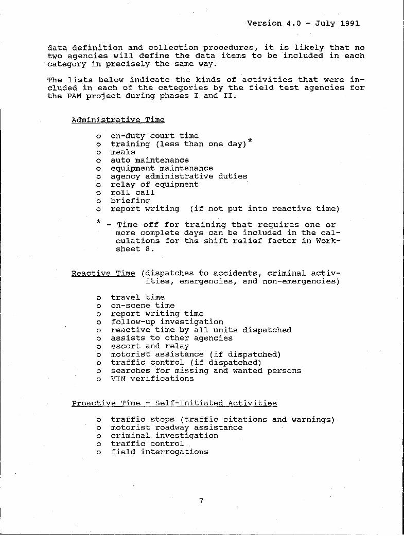
The lists below indicate the kinds of activities that were included in each of the categories by the field test agencies for the PAM project during phases I and II.
Administrative Time
o o o o o o o o o o
on-duty court time * training (less than one day)
meals auto maintenance equipment maintenance agency administrative duties relay of equipment roll call briefing report writing (if not put into reactive time)
* - Time off for training that requires one or more complete days can be included in the calCUlations for the shift relief factor in Worksheet 8.
Reactive Time (dispatches to accidents, criminal activities, emergencies, and non-emergencies)
o travel time o on-scene time o report writing time o follow-up investigation o reactive time by all units dispatched o assists to other agencies o escort and relay o motorist assistance (if dispatched) o traffic control (if dispatched) o searches for missing and wanted persons o VIN verifications
Proactive Time - Self-Initiated Activities
o traffic stops (traffic citations and warnings) o motorist roadway assistance o criminal investigation o traffic control o field interrogations
7
-l

Version 4.0 - July 1991
Proactive Time - Uncommitted Patrol
o patrolling assigned roadways (includes both moving and stationary patrol)
The ability to tailor the PAM procedures to reflect the particular data collection practices of an agency is a strength of the model; that is, rather than requiring an agency to redefine existing data collection procedures to "fit" the model, it is possible to tailor the PAM model to fit each agency. At the same time, however, the flexibility that such tailoring permits requires that caution must be used when comparing the staffing estimates produced by the PAM model for di.lferent agencies; that is, unless both agencies are including the same data items, defined in the same way, in each activity category, it may not be possible to reliably determine the underlying causes for differences in staffing estimates between the agencies.
Experience to date indicates the decision about which of the four categories each activity is assigned to has a relatively small impact on the final total staffing estimate. Far more important than the question of which category to use for each workload item is the need to insure that all trooper patrol workload activities are included and accounted for somewhere in the PAM model.
Selecting Autonomous Patrol Areas (APAs)
The PAM model estimates the total staffing for an agency by first determining the staffing levels for patrol areas using the following steps:
o The entire state (or part of a state) is subdivided into a number of autonomous patrol areas. The APAs must cover the entire state (or area of interest) and not overlap.
o The PAM model is used to determine the staffing level for each APA.
o The individual APA results are added together to obtain the staffing requirement for the entire state (or area of interest).
The selection of the APAs is dictated by the requirement that each APA should exhibit the following characteristics:
o virtually all of the CFS that originate in the APA are handled by troopers assigned to the APA or, conversely, almost none of the CFS that originate in the APA are handled by troopers assigned to areas outside of the APA;
8
'~----I
Version 4.0 - July 1991
o Troopers assigned to the APA are rarely dispatched to CFS outside of the APA; and
o Although troopers may be assigned to patrol specific subdivisions within the APA, troopers are routinely dispatched, as needed, to CFS anywhere within the APA.
The first two characteristics define what is meant by "autonomous." simply stated, it means that the APA must be, for the most part, a self-contained or independent operational area with little or no cross-over of personnel either into or out of the area. (As a guideline, 90% of the CFS in the APA should be handled by units assigned to the APA.)
The third characteristic indicates that the APA cannot itself be a collection of smaller APAs; that is, all of the units assigned to the APA must routinely be dispatched to CFS throughout the APA. If this is not the case; that is, if units are only dispatched to CF'S within their patrol areas and are rarely dispatched to CFS in other parts of the APA, then consideration should be given to dividing the APA into several smaller APAs.
The size of each APA within a state will vary depending on workload, popu.lation density! and traffic volume. To illustrate differences in the size of APAs, two examples taken from the Phase I field test, are described below. Each is based on a state agency that divided their entire state into individual APAs. Although the states differ considerably in size and population, in both cases the median-sized APA had an area of approximately 1,000 square miles (i.e., if shaped like a square, each side of the APA would be 31.6 miles long). In both states, smaller APAs were clustered around major metropolitan areas and larger APAs were used for less populated, rural areas.
state Agency Example #1. The first example is a midwestern state with a total population of 3.5 million persons and a total area of approximately 69,000 square miles. The state is divided into 8 troop districts which cover 114 counties. The 8 districts are further subdivided into 95 troop zones which were used to define 69 APAs (every APA consisted of either one or two zones). In terms of area, the median-s'ized APA covered 946 square miles (i.e., a square with each side equal to 30.8 miles). The smallest APA covered 205 square miles (14.3 miles on a side) and the largest had an area of 2,321 square miles (48.2 miles on a side). Half of all of the APAs had areas between 689.5 square miles (26.3 miles on a side) and 1,260.3 square miles (35.5 miles on a side).
state Agency Example #2. The second example is a large western state with a total population of more than 29 million and a total area of more than 156,000 square miles. The entire state is aivided into 8 patrol divisions which are furthered subdivided into 98 patrol zones. Each patrol zone was defined as an APA.
9
Version 4.0 - July 1991
The median-sized APA covered 1,083.5 square miles (32.9 miles on a side). The smallest APA was only 84 square miles (9.2 miles on a side) and the largest APA had an area of 10,557 square miles (102.7 miles on a side). Half of all of the APAs had areas between 559 square miles (23.6 miles on a side) and 1,843 square miles (42.9 miles on a side).
Worksheet options and the Use of Performance Standards
To provide as much flexibility as possible, four of the worksheets in the Manual give the user two or three different ways to derive a particular value. The decision about which option to use in each case is based on the availability of historical data and the desire of the agency to set an operational performance standard as a matter of policy.
Occasionally, first-time PAM l,i'sers are disappointed to learn that all of the PAM calculations are not based on historical data and/or "national" standards for staffing or workload. (No such national standards exist.) Although, it is theoretically possible to use the PAM model based entirely on historical data, this is rarely done for at least two reasons. First, it is very difficult to collect all of the required data, and secondly, use of historical data in all of the worksheets will yield staffing totals, assuming the model is valid and accurate, that will replicate the current staffing levels of an agency. While this may be useful in verifying the validity of the model, it is usually more likely that agencies are interested in examining the impact on staffing levels if one or more of the current workload, performance, or other data items are altered.
The remainder of this section briefly outlines the options explicitly available to the user in the worksheets. It should be noted that the term "explicitly" is used to highlight the fact that the user, in fact, "implicitly" has options in determining every data item required by the model (i.e., the value used for each item can be selected by policy or can be based on historical data). For each of the options identified below, the decisions of the Phase I field test agencies regarding which option was selected and the average value selected or derived for each are shown in Table 1. (The data presented in Table 1 is based on 35 applications of the PAM procedures by the seven active Phase I field test agencies; that is, the PAM procedures were used for 35 different APAs.)
Administrative Time Per Trooper (Worksheet 2). Worksheet 2 permits the user to use either of two options (Section 2.1 or section 2.2) to derive the average number of minutes per hour per trooper to be spent on administrative activities. section 2.1 allows the user to set the average number of minutes as a matter of policy. Section 2.2 directs the user through the process of deriving the value based on historical data. Table 1 indicates that among the 35 field test applications during Phase I, 19 were
10
I

Table 1
VALUES USED FOR SELECTED PAM INPUT DATA ITEMS
1999 Phase I Field Test, Seven Agencies (35 Worksheet Applications)
Worksheet Data Item Number of units of section (Worksheet Locationl At)J:~l i~gj:.i QD~ Measuremel)t Averaqe Minimum Maximum
2.1 Administrative Time 19 Min/Hr/Trooper 10.83 5.00 22.00 Policy (2.1)
2.2 Administrative Time 16 Min/Hr/Trooper 15.99 7.46 23.06 Historical (2.2.4)
...... ...... 3.1 Average Service Time 32 Hours/Accident 3.10 0.83 5.83 Accidents (3.1.2)
3.2 Average Service Time 31 Hours/CFS 1.66 0.60 13.63 Other CFS (3.2.2)
4.1 Self-Initiated Time 5 Min/Hr/Trooper 24.60 20.00 33.00 Policy - Direct (4.1)
4.2 Self-Initiated Time 7 Min/Hr/Trooper 10.60 10.20 13.00 Policy - Indirect (4.2.7)
4.3 Self-Initiated Time 23 Min/Hr/Trooper 11.57 4.88 16.72 Historical (4.3.4)
5.1 Controlled-Access Highways 27 Hours/Week 163.85 112.00 168.00 Coverage (5.1.2.2)
L~ ___________________________ _

Table 1 (continued)
VALUES USED FOR SELECTED PAM INPUT DATA ITEMS
1989 Phase I Field Test, Seven Agencies (35 Worksheet Applications)
Worksheet Data Item Number of units of Section (Worksheet Location) Applications Measurement Average Minimum Maximum
5.1 Controlled-Access Highways 27 Miles/Hour 43.33 21.00 60.00 Patrol Speed (5.1.2.3)
5.1 Controlled-Access Highways 27 Hours 1.12 0.30 4.00 Patrol Interval (5.1.2.4)
..,:... N 5.1 Primary Highways 30 Hours/Week 148.40 112.00 168.00
Coverage (5.1.3.2)
5.1 Primary Highways 30 Miles/Hour 33.58 19.50 50,,00 Patrol Speed (5.1.3.3)
5.1 Primary Highways 30 Hours 3.75 0.30 24.00 Patrol Interval (5.1.3.4)
5.1 Secondary Highways 28 Hours/Week 129.00 56.00 168.00 Coverage (5.1.4.2)
5.1 Secondary Highways 28 Miles/Hour 30.38 20.00 50.00 Patrol Speed (5.1.4.3)
5.1 Secondary Highways 28 Hours 66.59 1.00 168.00 Patrol Interval (5.1.4.4)

Table 1 (continued)
VALUES USED FOR SELECTED PAM INPUT DATA ITEMS
1989 Phase I Field Test, Seven Agencies (35 Works'!ae~;t Applica.tions)
Worksheet Data Item Number of units of section il'1orksheet Location) APMicati~ns Measu~elllent Averaq~ Minimum Maximum
5.2 Patrol Availability 27 % of calls 94.77 85.00 99.9 Immediate Response (5.2.6)
5.3 Area Patrol 3 Miles/Hour 46.67 40.00 55.00 Response Speed (5.3.4)
...... w 5.3 Area Patrol 3 Minutes 13.33 10.00 15.00
Response Time Goal (5.3.5)
5.4 Line Patrol 24 Miles/Hour 45.63 40.00 50.00 Response Speed (5.4.4)
5.4 Line Patrol 24 Minutes 13.77 3.00 20.00 Response Time Goal (5.4.5)
6.2 Two-Trooper Patrols (6.2.1) 14 Percent of units 25.00 25.00 25.00
7.1 Field Supervision 31 No. of Troopers 8.35 10.00 5.00 Span of Control (7.1.1) per Supervisor
7.1 Field Supervisor Time 31 Percent Time 8.65 0.00 50.00 on Patrol (7.1.2) on Patrol

Table 1 (continued)
VALUES USED FOR SELECTED PAM INPUT DATA ITEMS
1989 Phase I Field Test, Seven Agencies (35 Worksheet Applications)
Worksheet Data Item Number of Units of section (Worksheet Location) Applications Measurement Averaqe Minimum Maximum
B.2 Trooper On-Duty 31 On-Duty Hrs 1,769.72 1,650.00 1,930.00 Time (B.2.3) per Year
per TZ'ooper
8.4 Staff and Command 5 No. of Staff 6.00 1.00 10.00 I-' Policy (8.4) and Command ~
Personnel
8.5 Staff and Command 12 Ratio of 0.14 0.09 0.21 Historical (B.5.3) Troopers and
Field Super. to Staff and Command

Version 4~0 - July 1991
based on section 2.1 (Policy) and 16 were based on section 2.2 (Historical Data). The average time based on historical data, 15.99 minutes per hour per trooper, was considerably higher than the average of 10.83 minutes per hour per trooper based on policy.
Self-Initiated Time Per Trooper (Worksheet 4). Worksheet 4 permits the user to use anyone of three options (Section 4.1 or section 4.2 or section 4.3) to derive the average number of minutes per hour per trooper to be spent on self-initiated activities. section 4.1 allows the user to set the average number of minutes directly as a matter of policy. section 4.3 directs the user through the process of deriving the average value based on historical data. (Sections 4.1 and 4.3 parallel the options provided in sections 2.1 and 2.2 in Worksheet 2.) The third option, described in section 4.2, is a combination of the options available in 4.1 and 4.3. The derived value is based both on a policy decision (i.e., the average number of self-initiated contacts per shift per trooper) and the average time spent on each contact based on historical data. During the field test, the majority of applicat:ons determined self-initiated time based on historical experience (23 out 35 applications, see Table 1). Table 1 also indicates that the average value based on policydirect (24.60 minutes per hour per trooper based on 5 applications) was much higher than the average value based either on policy-indirect (10.60 minutes based on 7 applications) or historical data (11.57 minutes based on 23 applications). Some field test agencies were hesitant to use the policy options since they could be interpreted to be enforcement quotas.
Patrol Availability (Worksheet 5). Worksheet 5 permits the user to use anyone of three options (Section 5.2 or section 5.3 or section 5.4) to determine the number of on-duty troopers needed per day for "patrol availability." This value is then combined with the average number of troopers needed for "patrol visibility" (Section 5.1) to derive a total number of on-duty troopers needed per day for "proactive-patrol." section 5.2 is used to determine the number of troopers needed in order to have enough units available to respond immediately to a specified percentage (provided by the user) of all accidents and CFS. Sections 5.3 and 5.4 both determine the number of troopers required based on an average travel time requirement set by the user. section 5.3 is used for area patrol (i.e., when units have responsibility for responding to calls throughout a geographic area) while section 5.4 is used for line patrol assignments (i.e, when units have responsibility for a specific highway segm~nt only). Table 1 indicates that most applications (i.e., 27 out of 35) for the Phase I field test used section 5.2.
Number of Staff and Command Personnel (Worksheet 8). Worksheet 8 permits the user to determine the number of staff and command personnel required in addition to troopers and field supervisors for an APA. The PAM model gives the user two options for deriving this value. In Section 8.4, the number of staff and
15

Version 4.0 - July 1991
command personnel is based on policy. (This option parallels the policy choices available in sections 2.1 and 4.1). In section 8.5, the number of staff and command personnel is derived based on current agency practice. To use this option, the user must indicate the current number of staff and command personnel and the current number of troopers and field supervisors in the APA. A review of the field test results for Phase I indicates that many applications did not use sections 8.4, 8.5, and 8.F in Worksheet 8 (only 17 of the 35 applications). Of the 17 applications, 12 were based on historical experience (Section 8.5).
strategies for Controlling the Data Collection Effort
Use of the PAM model for one APA can vary in difficulty depending on the availability of data and the amount of work required to obtain the data. When all of the APAs for a state or for even part of a state are considered, the magnitude of the data collection effort required may be significant. The field test experience revealed two strategies that agencies can use to limit this effort.
APA-Independent Data. There are a number of input data items required in the model that are largely independent of the location or other attributes of each APA, and as a result, it may be possible to use one value for each data item for all APAs. Although the specific data items will vary from one agency to another, the following list should apply to most:
o average number of on-duty hours per year per trooper,
o average number of troopers per field supervisor,
o average fraction of time spent on patrol by field supervisors,
o average service time for accidents,
o average service time for other CPS,
o percent of units with two troopers,
o average time per hour spent on administrative activities per trooper
o average time per hour spent on self-initiated activities per trooper, and
o shift length.
APA-Dependent Data. There are also a number of input data items that will vary by APA within the same state. A partial
16
I

version 4.0 - July 1991
list would include:
o number of roadway miles by highway type,
o number of accidents and other CFS,
o amount of patrol coverage by highway type,
o average patrol speed by highway type,
o patrol interval by highway type,
o immediate response percentage,
o average response speed,
o average travel time,
o amount of patrol available from troopers on special assignment, and
o presence and influence of minimum staffing limits.
Several of the Phase I field test sites were able to control the data collection effort for APA-dependent data by recognizing that most of the data items that vary by APA are related to the proximity of the APA to urban or rural areas. Recognizing this, groups of APAs were categorized by their "urbanicity" and identical input data values were used for all APAs in the same category. Both of the state agency examples discussed above in terms of the number and size of APAs used this strategy.
State Agency Example #1. This agency divided its 69 APAs into four categories. The name and definition of each category are given below:
o Major Metro APAs which contain major freeways and arterials within high density populations areas. APAs are characterized by continual heavy congestion, high ADTs, high demand for field services, and wide ranging traffic congestion. Surface street arterials are characterized by periodic heavy traffic congestion, high ADTs, and are primary corridors for commuter traffic.
o Large Urban APAs are characterized by moderate to heavy well-defined popUlation centers (25,000 and above), diverse commercial and/or industrial activities, and cyclical congestion on a localized basis. Population centers are typically surrounded by large expanses of open land. Population centers may not necessarily be in the APA, but their location adjacent to the APA appreciably effects the traffic flow and congestion in the APA.
17
--~.------------------------------------
Version 4.0 - July 1991
o Moderate Urban APAs having one or more autono-mous mid-size population centers (10,000 to 25,000) with a large proportion of the region being rural. Industrial and/or commercial operations have a limited impact on these areas but there is some congestion.
o Rural APAs characterized as predominantly rural and having no population center greater than 10,000.
Table 2 below summarizes some of the attributes of each of the APA categories. Note that rural APAs have larger areas and contain more highway miles.
state Agency Example #2. This agency divided its 98 APAs into seven categories. The name and definition for each category are described below. Attributes of each of the APA categories are presented in Table 3.
o Metro Freeway Areas contains major freeways within high density major population areas and/or regional employment centers. Characterized by continual heavy congestion, high ADT, extremely high demand for agency services, and wide ranging congestion.
o Metro Freewav and Surface Street Areas contains major freeways and arterials within significant, high density, major population areas and/or regional employment centers. Characterized by continual heavy congestion, high ADT, extremely high demand for agency services, and wide ranging congestion. In addition, surface street arterials are characterized by periodic heavy congestion, high ADTs, and are primary corridors for commuter traffic.
o Major Urban Areas characterized by moderate to heavy population densities that are geographically dispersed. The arterials are periodically congested on a daily basis. They are generally cities and/or suburban areas that support commercial and/or industrial activity. Urban areas usually support metropolitan areas. These areas have a high demand for agency services.
o Moderate Urban and Rural Areas characterized by a large urban area supported by moderate to heavy, well-defined population centers, diverse commercial and/or industrial activities which experience cyclical congestion on a localized basis. Population centers are typically surrounded by large expanses of open land. These areas have a moderate demand for agency services.
18
I

version 4.0 - July 1991
Table 2
APA CATEGORY CHARACTERISTICS, STATE AGENCY EXAMPLE #1
Average Per APA
APA Length Number of Category No. of Area of Side Highway
Label APAs (square miles) (miles) Miles
Major Metro 6 448.1 21.2 257.7 Large Urban 9 948.1 30.8 482.8 Moderate Urban 12 979.8 31.3 453.4 Rural 42 1,093.8 33.1 495.9
TOTAL 69 998.9 31. 6 466.1
Table 3
APA CATEGORY CHARACTERISTICS, STATE AGENCY EXAMPLE #2
Average Per APA
APA No. Area Length Number of Category of (square of Side Highway
Label APAs miles) (miles) Miles Population
Metro Freeway 3 101. 3 10.1 81.4 951,333 Metro Freeway & 6 265.3 16.3 416.5 1,016,850
Surface Street Major Urban 13 458.3 21.4 655.2 784,262 Moderate Urban 16 1,496.0 38.7 1,247.5 351,713
& Rural Minor Urban & 12 1,431.1 37.8 922.8 146,855
Rural Rural with 32 1,920.0 43.8 967.2 70,405
Major Arterials Rural without 16 2,881.7 53.7 1,184.5 42,524
Major Arterials
TOTAL 98 1,597.0 40.0 940.8 300,750
19

version 4.0 - July 1991
o Minor Urban and Rural Areas characterized by having one or more autonomous population areas. Industrial and/or commercial operations have a limited impact on these areas and there is little congestion. Urban portions have minimal impact on demand for agency services.
o Rural Areas with Major Arterials characterized by having one or major arterials and intermittent population centers which have little or no impact on agency operations.
o Rural Areas without Major Arterials character-ized by having intermittent population centers which have little or no impact on agency operations.
within each category, uniform values were established for the following input data items:
o hours of patrol coverage by highway type,
o patrol interval time (hours) by highway type,
o average travel time (minutes),
o percent of accidents and other CFS for which a unit is immediately a'railable, and
o percent of units wi'th two troopers.
Discussion of Individual Data Items
The PAM model estimates the required staffing level for an APA by accounting for all of the time that troopers need to perform their patrol activities. The PAM model (Version 4.0) uses four time categories and general definitions about what activities are associated with each category. It is important to note, however, that the current model represents only one way out of many that could be used to categorize and define trooper activities. The significance of this observation is that regardless of what categories and definitions are used, they must account for all trooper activities. As expected, the Phase I field test provided the project team with considerable feedback about a number of data definition and data collection issues. This section provides an overview of some of the data-related issues tha't arose during the field test.
Highway types. The PAM worksheets identify three highway types: controlled-access, primary, and secondary. These categories are used in Section 5.1 for the derivation of the number of on-duty troopers needed each day to meet the patrol interval objectives set by the user for each highway type. PAM users are
20

Version 4.0 - July 1991
not required to use these particular roadway categories. To accommodate particular data collection procedures that are used within their state and agency, users may want to use different definitions for highway types and a different number of highway types. The critical issue is not whether three highway types are used or whether the definitions match those used in the worksheets, but rather that all highway types and miles routinely patrolled in the APA are included in ";;he procedures for deriving agency staffing estimates.
Immediate response percent. The immediate response percent is used in Section 5.2 to determine how many on-duty troopers are needed each day to insure that a trooper will be available for immediate assignment for a given percent of all accidents and other CFS. It is important to note that "immediate" response is not the same as "rapid" response. Immediate response merely implies that at least one trooper will be available, somewhere in the APA, for the assignment. No consideration is give to how far away the trooper may be from the incident. Users that are interested in the number of troopers that are needed to maintain a user-specified average travel time in responding to incidents should use either section 5.3 or section 5.4. Table 1 indicates that the immediate response option in section 5.2 was used in 27 of the 35 field test applications and the average value selected was approximately 95 percent.
On-dut~ hours per year per trooper. The average number of on-duty hours per year per trooper is used in Section 8.2 to calculate the "shift relief factor" (SRF). The shift relief factor indicates how many troopers are needed to cover one shift position every day. For a-hour shifts, SRFs typically range from 1.60 to 1.90; i.e., for each shift position, a total of 1.6 to 1.9 troopers is needed. A common question is whether the average number of on-duty hours per year per trooper equals 2,080 hours which is obtained by multiplying 52 weeks by 40 hours per week. The answer to this question is no. The 2,080 hours equals the number of hours for which a trooper is "paid" for one year and is greater than the number of on-duty hours because it includes paid "time off" (e.g., vacations and holidays). The average number of on-duty hours per year per trooper is based on the number of hours each trooper actually appears for duty, not on the number of hours for which the trooper is paid. Although it is easy to see why "benefit time off" like vacations and holidays should not be included, there are other situations in which the definition of lion-duty" time is more difficult to interpret. As an example, consider a trooper who is sent to a two-week training program. Should the time spent on training be counted as "on-duty" time? The answer may depend on who is answering the question. An administrator may argue that the trooper is "on-duty" whether he/she is on patrol or at a training program. A district commander, on the other hand, may argue that when the trooper is gone for two weeks, there is a staffing shortage on patrol that is just as real as if the trooper were on a two-week vacation. From the commander's point of view, the trooper is not lion-duty"
21
~----------------------------------------------------------------.--------------.--- --

version 4.0 - July 1991
in the sense that he/she is not on patrol, and as a result, the two weeks spent at training should not be included as on-duty time. There is no one "right" way to define on-duty time; it depends on the policies and practices adopted by each agency. Since the definition used to calculate SRFs may vary from one agency to another, the following guidelines should be noted:
o The calculation of the shift relief factor in Section 8.3 requires that a definition of lion-duty" time, appropriate for the agency, be adopted; and
o The comparison of shift relief factors for different agencies is not appropriate unless the same definition of "on-duty" time is used by both agencies.
Table 1 indicates that the average value for on-duty time per year per trooper was 1,770 hours which, assuming 8-hour shifts, produces a SRF·of 1.65 troopers per shift position.
Patrol coverage. Patrol coverage is used in section 5.1 to calculate the number of on-duty troopers required each day to meet a user-specified patrol interval. Patrol coverage refers to the number of hours per week that an agency will provide services in an APA or on a highway segment. (The maximum coverage is 168 hours per week.) Patrol coverage is a policy decision and represents an either-or situation (i.e., either coverage is prov~ded or it is not). Patrol coverage does not identify the level or intensity of coverage for a particular area; this is indicated by the "patrol interval" discussed below. Table 1 indicates that patrol coverage differed considerably by highway type for the field test agencies. For controlled-access highways, the average was 163.85 hours per week; for primary highways, the average was 148.40 hours; and for secondary highways, the average was only 129.00 hours.
Patrol interval. Patrol interval is used in section 5.1 of the Manual as a measure of the level or intensity of patrol coverage. It is measured in hours and indicates the average length of time that a stranded motorist would have to wait to see a trooper come by on free patrol (i.e., proactive-patrol). As an example, a patrol interval of one hour means that a motorist, stranded on the roadway, would have to wait an average of one hour before seeing a trooper. While there is no theoretical upper limic to the patrol interval, the largest value used during the field test was 168 hours (i.e., a motorist would have to wait for one week). Table 1 indicates that the average patrol interval for controlled-access highways for the field test was only 1.12 hours. For primary highways, the average was 3.75 hours, and for secondary highways, the average was 66.59 hours.
Patrol speed. Patrol speed is used in section 5.1 as part of the calculation to determine the number of on-duty troopers required to meet a specified patrol interval. Average patrol speed and average response speed (discussed below) are often
22
Version 4.0 - July 1991
among the most difficult data items to obtain for use in the PAM model. A number of different approaches can be used to estimate this value:
o Use of log sheets. Average patrol speed equals the total number of miles driven while on "patrol" divided by the total time spent on "patrol." The mileage and time estiIP"'\tes must be based on "proactive-patrol" as defined in the PAM model; that is, only mileage and time spent on free patrol (including stationary patrol). Any mileage accumulated for or time spent on activities that fall into any of the non-patrol categories (i.e.; administrative, reactive, and self-initiated) is not included.
o Ride alonq observers. Some agencies have attempted to estimate average patrol speeds by having observers ride along with troopers while on patrol. Experience indicates, however, that the presence of an observer may cause changes in driving behavior.
o Survey of troopers. Another approach is to survey troopers to obtain an estimate of the average speed. Use of this method, however, is often questioned since experience indicates that human recollection is not reliable in estimating "average" speeds. (There is a tendency to only remember the cruising or top speed and to forget times when a unit is either stationary or moving very slowly.)
In the last section of the Guide, a general approach to using the PAM model is outlined One of the key points is t.hat users must exercise judgment in determining how accurat.e each input value should be and how much effort should be expended in obtaining each item. Patrol speed is a data item which can, if one is not careful, require far more effort than may be justified by its contribution to the final staffing estimates. In Table 1, the average patrol speeds used by the field test agencies were 43.33 MPH for controlled-access highways, 33.58 MPH for primary highways, and 30.38 MPH for secondary highways.
Response speed. Response speed is used in sections 5.3 and 5.4 to estimate the number of on-d\~ty troopers required to provide a response capability which maintains a user-specified average travel time. Like patrol speed, this data item may be quite difficult to obtain. The same procedures that were outlined above for determining patrol speeds can also be used to estimate response speeds with all of the corresponding difficulties associated with each of the procedures. (If log sheets are used, mileage and times must be based on travel to reactive incidents only.) In fact, the influence of ride-along observers and the unreliability of personal recollection to estimate response speeds may be even more pronounced. PAM users are strongly encouraged to follow the recommended data collection strategy
23

Version 4.0 - July 1991
outlined in the last section of the Guide to avoid unnecessary effort spent on obtaining response speed estimates. In Table 1, the average response speed (over all highway types) is 46.67 MPH for area patrol and 45.63 MPH for line patrol.
Self-initiated time. Worksheet 4 is used to determine the average number of minutes per hour per trooper for self-initiated activities. In PAM, self-initiated activities refer to activities initiated by a trooper rather than directed by the dispatching center. It is important to note that the distinction between reactive and self-initiated activities is not determined by what is done but rather by the manner in which the activity is initiated. As an example, if a trooper is directed to a particular location to control traffic because of a fallen tree on the roadway, the time spent on this activity would be charged to reactive time. If, on the other hand, the trooper discovers the fallen tree while on free patrol and determines that he/she should control traffic until the tree can be removed from the roadway, this time would be assigned to the self-initiated category. In Table 1, the average self-initiated time selected by policy was 24.60 minutes per hour per trooper. When based on a specified number of contacts per shift and the average time per contact, the average self-initiated time was only 10.60 minutes per hour per trooper. When based solely on historical data, the value was 11.57 minutes per hour per trooper.
Service time. Average service times for accidents and other CFS are used in Worksheet 3 to determine the average number of on-duty troopers needed each day to handle the "obligated" workload. Service time refers to the total spent on an incident by all agency patrol personnel. Service times should include:
o travel time (not including dispatching time),
o on-scene time,
o report writing time,
o investigation time (by patrol) ,
o processing time (e.g., for DUIs) , and
o time spent by backup units.
In Table 1, the average service times for accidents and other CFS are 3.J.0 hours and 1.66 hours respectively. Few agencies have data collection procedures that capture all of the components of service time listed above. Many CAD systems, for example, will capture the travel, on-scene, and possibly some follow-up time of the primary unit dispatched to an incident, but may not capture report writing and time spent by backup units. Some agencies do not routinely record the frequency and amount of time spent by backup units despite the fact that backup time can represent a significant proportion of the total obligated time for an agency.
24

version 4.0 - July 1991
If an agency plans to use operational data captured by a CAD system, it is recommended that the specific definitions built into the system be examined to detect possible shortcomings in the data summaries produced by the system. Recognizing that few agencies routinely capture all of the components of service time, it is likely that most PAM users will have to estimate all or part of the average service times that they use in the PAM model. Reliable estimates for average service times do not require that information be obtained from all incidents. (In fact, this is not realistic since incident records are often incomplete.) A reliable value for the average service time for a particular incident category can be obtained by randomly drawing a sample of 100 or more incidents in the category for the time period of interest.
In Worksheet 3, total obligated time for an agency is determined first by calculating the total obligated time required for all accidents and then using that time to determine the total number of on-duty troopers needed each day to handle accidents (Section 3.1). The same procedure is used in section 3.2 to determine the total number of on-duty troopers required each day to handle all other CFS. The results are then added together in Section 3.3 to obtain the total number of on-duty troopers needed each day for both accidents and other CFS. The PAM model separates accidents and other CFS to enable the user to explicitly identify the number of troopers required for each type of incident. Some agencies, however, did not use both categories in Worksheet 3, but decided instead to group all incidents in either the accident or the other CFS category. This procedure will yield the same total. number of on-duty troopers if an adjusted average service time based on both types of incidents is used. Similarly, more than two categories can be used. For example, the collection of all "other CFS" can be divided into several subcategories and each subcategory can be used to determine the number of on-duty troopers that are needed each day to handle all of the calls in that subcategory. (To use this procedure, however, requires that an average service time must be estimated for each subcategory.) The total number of troopers required is obtained by adding the trooper requirements for each subcategory together. While the use of subcategories provides additional information about which types of incidents require the most personnel, it has no impact on the total staffing level required for all incident types collectively. As a result, the value of the additional information must be weighed against the extra effort required to collect incident data by subcategory and to estimate an average service time for each.
Shift length. The PAM procedures are designed to accommodate any shift length (e.g., 8 hours, 10 hours, or 12 hours). Changes in the shift length will alter the shift relief factor for an agency. For 8-hour shifts, SRFs typically fall into the range 1.60 - 1.90. For 10-hour shifts, the range is 2.00 - 2.40; and for 12-hour shifts, the usual range is 2.40 - 2.90. A common misperception is that since a change in the shift length changes
25

version 4.0 - July 1991
the SRF, it must also change the total staffing requirement for an agency. This is not true. In fact, if the average work week (e.g., 40 hours per week) and the total time off given for benefits (e.g., vacations, holidays, etc.) remain the same, a change in shift length has no impact on total staffing.
Special assignment personnel. Special assignment personnel who are also used for patrol can be included in Worksheet 7 of the Manual. For each type of special assignment, the user must provide the total number of troopers used for that assignment in the APA and the average fraction of time each trooper spends on patrol. This information is then used to adjust the total number of "non-special assignment" troopers that are needed and the fitl.al staffing value from Worksheet 7 includes both the special and non-special assignment troopers. The PAM model, however, cannot be used to estimate how many troopers will be needed for special assignments (e.g., weights, hazardous materials, etc.).
Staff and command personnel. Section.s 8.4, 8.5, and 8.6 in the Manual c',n be used to estimate the number of staff and command personn:el required for an APA. It is. not necessary, however, to use these sections to obtain estimates for the number of troopers and field supervisors that are required. The usefulness of these section depends to some degree on how the APAs in a jurisdiction are defined. If each troop district (i.e., an area headquarters that provides command and administrative support for several counties) for an agency is treated as one APA, the results obtained from sections 8.4, 8.5, and 8.6 can be used directly. If, however, each district is divided into several APAs, it may be difficult to assign district-level staff and command personnel to individual APAs. In this case, the aggregate total of the staff and command personnel in the APAs may not accurately reflect the total number required for the district.
Travel time. In sections 5.3 and 5.4, the PAM user is required to provide a travel time objective as part of the procedure for determining how many on-duty troopers are needed for either area or line patrol. Travel time refers to the time interval that begins when a trooper receives a dispatch and ends when he/she arrives on scene. Travel time does not include dispatching time (i.e., the time required at the communication center to process and transmit the assignmenL to the trooper). It is also important to note that the travel times required in sections 5.3 and section 5.4 are "averages." This means that the actual travel time will be less than the user-specified average about half of the time and greater than the average for the other half. In Table 1, the average travel time objective selected for the field test were 13.33 minutes for area patrol and 13.77 minutes for line patrol.
26
I

version 4.0 - July 1991
SECTION 4: Recommended Data Collection and Implementation Procedure
The bulk of the work associated with using the PAM procedures involves defining and collecting data, and unless caution is exercised, it is possible to be overwhelmed by these activities. This section of the Guide presents a recommended procedure for using the PAM model that is designed to avoid excessive data collection efforts. The basis for the recommended procedure is the observations, successes, and problems encountered by the seven state agencies that actively participated in the Phase I field test process. The procedure consists of four steps that describe an iterative process for using the PM1 model.
STEP 1: Obtain Initial Staffing Level Estimates With Minimum Data Collection Effort
It is likely thQt every agency that uses the PAM procedures will find that it does not have all of the input data that is required. This may occur for several reasons: the agency does not routinely collect the data; the agency collects the data, but not in the form or categories required; or the data is collected but not stored in an easily retrievable form. Whatever the reasons, every agency will be faced with the question of how much effort to expend in obtaining each data item. step 1 recommends minimizing the initial data collection effort; that is, for input data items that are not easily obtained, "quick and dirty" estimates or guesstimates should be used. The ~ationale for this recommendation is that it is more important to obtain an initial estimate of the total staff than it is to obtain a high lev,sl of accuracy for every input data item. It is strongly recommended that plans for extensive data collection be deferred until steps 2 and 3 described below are implemented.
STEP 2: Assess the Quality of the Input Data Items
After the initial staffing estimates have been obtained, each of the input data items should be assessed in terms of completeness, reliability, and accuracy. The assessment of each data item will be, to some extent, a sUbjective process. As an example, it may be determined that the number of primary hightqay miles in an APA equals 368 miles. If this figure is obtained from the county or state highway department based on recent data, it can be concluded that this data item is fairly "strong." On the other hand, if the average service time for handling accidents is based on a survey of three field sergeants who give individual estimates of 2.1, 2.5, and 3.2 hours, it would be clear that further effort is needed to obtain a better estimate. It is recommended that all of the data items be placed into three or four groups depending on their relative quality (i.e., accuracy, reliability, etc.).
27
l
I

I
version 4.0 - July 1991
Those data items in the lowest category (i.e., least accurate, least reliable, etc.) will be the initial candidates for additional refinement.
STEP 3: Investigate the Sensitivity of the Staffing Estimates to Changes in Individual Data Items
The next step is to identify which of the "soft" input data items should be refined. The basis for identifying these items is to determine which items make the biggest contribution to the overall staffing estimate. Not all input data items in PAM are equally important. For example, in an agency that places a low priority on patrol visibility on secondary highways, it is not particularly important to have a very accurate figure for the number of secondary highway miles in the APA since a change of even 20 or 30 percent in the number of miles may only affect the final staffing estim.,tes by 1 or 2 percent. In contrast, final staffing estimates tend to be fairly sensitive to changes in the value used for the shift relief factor for an agency, and changes of only 3 or 4 percent in the relief factor can produce equallysized changes in the final staffing estimates. Sensitivity analyses should be done for each of the input data items in the lowest data quality categories to identify those items for which additional accuracy is needed.
STEP 4: Improve Accuracy of Important Data Items
The final step recommends that the input data items targeted for additional refinement be prioritized based on the results of steps 2 and 3 above. Such a list serves two purposes. First, effort can be directed toward those data items that are "soft" and, equally important, that are important to the final staffing figures. Secondly, limited resources can be targeted efficiently to insure that the maximum benefit in terms of the quality of the final results are obtained. As each input data item is improved f
more reliable staffing figures will be generated. Clearly, this process has no natural termination point, but rather is limited by the resources and time that are available. At some point, the effort and resources required to improve the input data values will outweigh the value gained by the changes in the overall staffing estimate.
28

version 4.0 - July 1991
APPENDIX A: Comprehensive List of Data Requirements for Use of the PAM Model
This appendix presents a list of all of the data items that may be used in the PAM model. The list is organized by the worksheet in which each item is first used.
Worksheet 1: Operations, Workload, and Highway Data
All of the data items in Worksheet 1 are required.
Data Item
Name of the APA . . . • • • • • • G
Shift length (hours)
Average number of on-duty hours per year per trooper . . . . .• ••••••
Average number of troopers to be supervised by each field supervisor . • . • • • . . . .
Percentage of field supervisor on-duty time spent on patrol, reactive, and self-initiated activities . . . . . . . • . . • • • . • • •
Patrol coverage per week (hours), controlled-access highways in the APA • . •
Average patrol speed (MPH), controlled-access highways in the APA . . . . . . . • • . • • •
Patrol interval performance Objective (hours), controlled-access highways in the APA • . . .
Patrol coverage per week (hours), primary highways in the APA . . . . . . . • . .
Average patrol speed (MPH), primary highways in the APA . . . . . . . . . . . . . . . .
A - 1
Worksheet Identifier
1.1
1.2.1
1. 2.2
1. 2.3
1. 2.4
1.2.5.1
1.2.5.2
1.2.5.3
1.2.6.1
1.2.6.2
--- --I
I
I
Version 4.0 - July 1991
Data Item
Patrol interval performance objective (hours), primary highways in the APA . . . . . • .
Patrol coverage per week (hours), secondary highways in the APA . . . • .. ...
Average patrol speed (MPH), secondary highways in the APA . . . . . . . . . . . . . . . . .
Patrol interval performance objective (hours), secondary highways in the APA . • • • • . . •
Total number of days in the workload sample period • . . • . . . • .
Total number of accidents handled by the agency during the sample period . . . . • . . . • .
Average service time (hours) per accident . .
Total number of other CFS handled by the agency
Worksheet Identifier
1.2.6.3
1.2.7.1
1.2.7.2
1.2.7.3
1.3.1
1. 3.2
1. 3.3
during the sample period . . • • • . •. 1.3.4
Average service time (hours) per CFS . . . . . . . 1. 3.5
Number of miles, controlled-access highways in the APA . . . . . . . . . . . . . Go • • 1.4.1
Number of miles, primary highways in the APA 1. 4.2
Number of miles, secondary highways in the APA 1. 4.3
Worksheet 2: Administrative Time
In Worksheet 2, the user has the option of providing data item 2.1 or data items 2.2.1 and 2.2.2.
Data Item
Administrative time performance objective in minutes per hour per trooper • . • .
A - 2
Worksheet Identifier
2.1
I
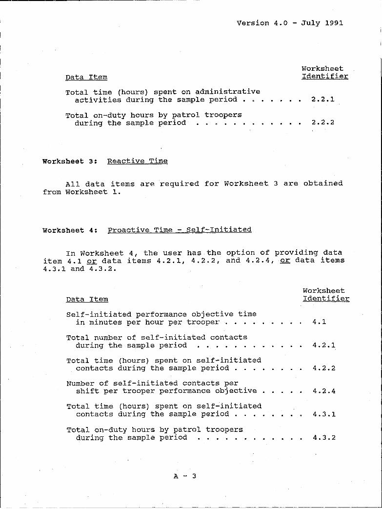
Version 4.0 - July 1991
Data Item
Total time (hours) spent on administrative activities during the sample period .
Total on-duty hours by patrol troopers during the sample period . . . • • •
Worksheet 3: Reactive Time
Worksheet Identifier
2.2.1
2.2.2
All data items are required for Worksheet 3 are obtained from Worksheet 1.
Worksheet 4: Proactive Time - Self-Initiated
In Worksheet 4, the user has the option of providing data item 4.1 ~ data items 4.2.1, 4.2.2, and 4.2.4, or data items 4.3.1 and 4.3.2.
Data Item
Self-initiated performance objective time in minutes per hour per trooper . . . •
Total number of self-initiated contacts during the sample period . . • . • .
Total time (hours) spent on self-initiated contacts during the sample period . . . •
Number of self-initiated contacts per shift per trooper performance objective .
Total time (hours) spent on self-initiated contacts during the sample period . .
Total on-duty hours by patrol troopers during the sample period • . . . . •
A - 3
· ·
· ·
· ·
· ·
· ·
· ·
· ·
· ·
Worksheet Identifier
4.1
4.2.1
4.2.2
4.2.4
4.3.1
4.3.2

version 4.0 - July 1991
Worksheet 5: Proactive - Patrol
In Worksheet 5, the user has the option of providing data items 5.2.2 and 5.2.6 or data items 5.3.2, 5.3.3, 5.3.4, and 5.3.5, or data items 5.4.2, 5.4.3, 5.4.4, and 5.4.5.
Data Item
Coverage per week for immediate response (hours) •.•••.
Performance objective percentage of accidents, CFS, and self-initiated activities for which there will be at least one trooper available
Coverage per week for area patrol (hours)
Area (square miles) of the APA
Average response speed (MPH)
Average travel time performance objective (minutes) . . . • .
Coverage per week for line patrol (hours)
Total highway miles to be patrolled in the APA
Average response speed (MPH)
Average travel time performance objective (minutes) . . • . .
Worksheet 6: Average Daily Number of On-Duty Troopers
Worksheet Identifier
5.2.2
5.2.6
5.3.2
5.3.3
5.3.4
5.3.5
5.4.2
5.4.3
5.4.4
5.4.5
In Worksheet 6, the user can provide data item 6.2.1 ~ data item 6.3.1.
Data Item
Percentage of time patrol units are staffed with two troopers . • . • •. ..••
A - 4
Worksheet Identifier
6.2.1

Version 4.0 - July 1991
Data Item
Average minimum number of on-duty troopers required per day for all patrol activities, based on agency policy . . . • • . . . • •
Worksheet 7: special Assignments and Field supervision
Worksheet Identifier
6.3.1
In Worksheet 7, the user has the option of using all, some, or none of the data items listed below.
Data Item
Name of special assignment 1
Average number of on-duty troopers on
Worksheet Identifier
7.2.1.1
specialized assignment 1 • . . . • . • . . • . • 7.2.1.2
Percentage of on-duty time spent on patrol by troopers assigned to special assignments 1 . . • •
Name of special assignment 2
Average number of on-duty troopers on
7.2.1.3
7.2.2.1
specialized assignment 2 . • . . • . • . • • • . 7.2.2.2
Percentage of on-duty time spent on patrol by troopers assigned to special assignments 2 . • . .
Name of special assignment 3
Average number of on-duty troopers on
7.2.2.3
7.2.3.1
specialized assignment 3 . • • . . • • • • • • • 7.2.3.2
Percentage of on-duty time spent on patrol by troopers assigned to special assignments 3 . . • .
A - 5
. . . . . . . . 7.2.3.3
l
J

version 4.0 - July 1991
Worksheet 8: Total Staff Requirements
In Worksheet 8, the user may provide data item 8.4 or data items 8.5.1 and 8.5.
Worksheet Data Item Identifier
Number of staff and command personnel -agency policy • . . • . . . • • • • • • • • • •• 8.4
Current number of troopers and field supervisors 8.5.1
Current number of staff and command personnel . .• 8.5.2
Worksheet 9: Allocation of Patrol Personnel Among Several APAs
Worksheet Data Item Identifier
Total number of additional personnel for all APAs (enter a negative value for personnel reduction) ..•
Total number of current personnel .
Number of current personnel in each APA .
Number of personnel estimated for each APA by the PAM model . . . .. •..•.
9.1.1
9.1. 2
9.1. 3
9.1. 5
supplemental Worksheet: Patrol Availability - Immediate Response
The Supplemental Worksheet for Section 5.2 is located in Appendix A in the Manual.
Data Item Identifier
Percent of on-duty staff on shift 1 · A. 2.1
Percent of on-duty staff on shift 2 · A.2.2
Percent of on-duty staff on shift 3 · A.2.3
A - 6
----------
I

Version 4.0 - July 1991
Data Item
Performance objective percentage of accidents, CFS, and self-initiated activities on shift 1 for which there will be at least one trooper available . . . . . . . . . . . . ft • • • • •
Performance objective percentage of accidents, CFS, and self-initiated activities on shift 2 for which there will be at least one trooper available . . . . . . . . . . . . . . . . . .
Performance objective percentage of accidents, CFS, and self-initiated activities on shift 3 for which there will be at least one trooper available . . . . . . tit • • • • • • • • • • •
A - 7
Worksheet. Identifier
A.6.1.1
A.6.2.1
A.6.3.1

version 4.0 - July 1991
APPENDIX B: Glossary and Worksheet Abbreviations and Notation
Glossary
Accident In PAM, an accident refers to a sequence of events involving one or more vehicles that produces injury, death, or property damage and requires investigative time by one or more troopers.
Administrative time Time spent by patrol personnel on activi-ties other than reactive, self-initiated, or patrol. May include supervision, meals, on-duty court time, auto maintenance, training, and agency administrative duties.
Agency policy The specification of performance objectives for use in the PAM model. (See "Performance Objective.")
Allocation In the PAM model, allocation refers to the distri-bution of a specified number of troopers over several APAs or several time periods.
Area - The geographic area of the APA in square miles. Large areas within the jurisdiction without roads (e.g., lakes, wilderness areas, etc.) should not be included. The area is used to determine the number of troopers needed to provide a specified average travel time to accidents and other CPS. The value used in the model may include areas outside of the jurisdiction of the agency if passage through these areas is routinely used in responding to accidents and other CPS.
Area patrol Patrol assignment which includes responsibility for both traffic services and general police response within a specified geographic area. (See "Line Patrol.")
B-1

Version 4.0 - July 1991
Autonomous patrol area (APA) - Patrol area in which one or more troopers are assigned which has the following characteristics: (1) CFS may be assigned to any of the troopers in the APA, (2) CFS are rarely dispatched to troopers assigned outside of the APA, and (3) troopers assigned to the APA rarely respond to CFS outside of the APA.
Availability In ' .. he Pl~ model, one criterion for determining the number of troopers required for patrol is based on an analysis of the number of troopers that must be "available" in order to meet two performance standards: (1) the likelihood or probability (set by the user) that at least one trooper will be available for immediate dispatch to a CFS, and (2) that enough troopers will be available to insure that a specified average travel time (set by the user) will be met.
Backup unit A patrol unit that is assigned or responds to a CFS to assist the primary unit.
Benefit days off Paid time off taken by officers in addition to regular days off provided by the work schedule. Benefit time off includes vacation leave, sick leave, holidays, and compensatory time off.
CFS CFS stands for "calls for service" (i.e., calls to the police agency which require the dispatch of one or more troopers). The PAM model uses the total time required to service CFS as the workload measure for reactive time. For state agencies with full police powers, CFS include criminal activities, traffic accidents, and various other police services. Highway patrol agencies may limit their reactive time to CFS which consist primarily of traffic aCl~idents and assistance to motorists and other agencies.
citation A summons or notice to appear issued by an officer for a traffic law violation.
Compensatory time off Time off granted in lieu of monetary payment for overtime work. Compensatory time or "comp time" may be granted at different rates. A straight time rate implies that one hour of comp time is given for each hour of overtime worked. A comp time rate of time and a half implies that 1 1/2 hours of comp time is granted for each hour of overtime.
B-2
I

Version 4.0 - July 1991
constrained allocation Constrained allocation refers to the distribution of a specific number of officers over several APAs with limitations on the number of officers that can be assigned to each APA. In the PAM model, constrained allocation is used for two cases: (1) when a specific number of officers are to be added to an existing allocation, the constrained allocation will determine a new allocation of the existing and new officers with the limitation or "constraint" that the revised staffing level for each APA must equal or exceed the existing level for each APA, and (2) when a specific number of officers are to be subtracted from an existing allocation, the constrained allocation will determine a new allocation of the reduced number of officers with the limitation or constraint that the revised staffing level for each APA must not exceed the existing staffing level for each APA. (See "Unconstrained Allocation. ")
contacts In the PAM model, contacts refers to self-initiated activities. One measure of the level of self-initiated activity is a count of the number of self-initiated contacts (i.e., the number of stops for traffic violations, warnings, and assists) per shift.
Controlled-access highway A highwa.y in which owners or occu-pants of abutting lands have no legal right of access to or from the highway except at such points only and in such manner as may be determined by the public authority having jurisdiction over the highway (e.g., most interstate highways). In the PAM model, the highway system is divided into three categories: controlled-access, primary, and secondary. The PAM user is not required to use all three categories and may, if desired, redefine the categories to insure compatibility with agency data.
Deployment plan A generic term that refers to the resource allocation staffing plan for an agency. A comprehensive deployment plan may indicate the level of staff resources that are needed and how those resources should be allocated by time (e.g., by time of day and day of the week) and by geography (e.g., by APA).
Deterrence The impact of visible patrol units on potential traffic and criminal offenders. (See "Preventive Patrol. ")
Dispatching time The time interval that begins when a call is received at the dispatching center and ends when the assignment is communicated to a trooper.
B-3
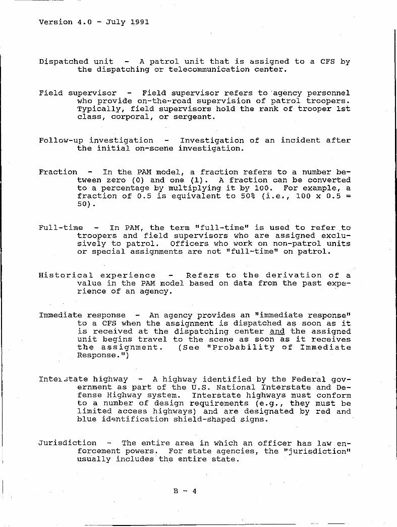
Version 4.0 - July 1991
Dispatched unit A patrol unit that is assigned to a CFS by the dispatching or telecommunication center.
Field supervisor Field supervisor refers to agency personnel who provide on-the-road supervision of patrol troopers. Typically, field supervisors hold the rank of trooper 1st class, corporal, or sergeant.
Follow-up investigation Investigation of an incident after the initial on-scene investigation.
Fraction In the PAM model, a fraction refers to a number be-tween zero (0) and one (1). A fraction can be converted to a percentage by multiplying it by 100. For example, a fraction of 0.5 is equivalent to 50% (i.e., 100 x 0.5 = 50) .
Full-time In PAM, the term "full-time" is used to refer to troopers and field supervisors who are assigned exclusively to patrol. Officers who work on non-patrol units or special assignments are not "full-time" on patrol.
Historical experience Refers to the derivation of a value in the PAM model based on data from the past experience of an agency.
Immediate response An agency provides an "immediate response" to a CFS when the assignment is dispatched as soon as it is received at the dispatching center and the assigned unit begins travel to the scene as soon as it receives the assignment. (See "Probability of Immediate Response.")
InteL~tate highway A highway identified by the Federal gov-ernment as part of the u.S. National Interstate and Defense Highway system. Interstate highways must conform to a number of design requirements (e.g., they must be limited access highways) and are designated by red and blue id~ntification shield-shaped signs.
Jurisdiction The entire area in which an officer has law en-forcement powers. For state agencies, the "jurisdiction" usually includes the entire state.
B - 4

Version 4.0 - July 1991
Line patrol Patrol assignment for which troopers are assigned exclusively to highway segments. (3ee "Area Patrol.")
Linear patrol Same as "Line Patrol."
Model The PAM model is a systematic procedure for representing the relationships between the staff requirements for state and provincial law enforcement a0encies and a number of workload, operational, and policy descriptors.
Moving patr?l Patrol time during which a patrol vehicle is mOVl.ng with the normal flow of traffic. (See "stationary Patrol.")
Non-patrol time In PAM, "non-patrol time" refers to on-duty time spent on special assignments.
Non-permanent assignment A temporary special assignment. (See "special Assignments.")
Non-supervisory work Work done by a field supervisor that does not involve the supervision of subordinates. Nonsupervisory work usually includes patrol activities that could be performed by troopers.
Obligated time The total time required by patrol units to respond to and service CFS. Obligated time includes the travel time, on-scene time, report writing time, and follow-up investigation time expended by all patrol units that respond to a CFS. In the PAM model, total obligated time is based on the time spent by each unit, not each officer. Total obligated time serves as the workload measure to determine the number of patrol units required for reactive time activities. Total obligated time is also referred to as total service time or total reactive time.
Officers A generic term that refers to sworn personnel in a law enforcement agency.
B - 5
l
I

Version 4.0 - July 1991
On-duty time In the PAM model, on-duty time refers to the actual time that an officer appears for work. Actual onduty time can be determined by assuming that an officer works every day and subtracting the number of days that an officer is off duty for both scheduled time off (i.e., regular days off) and benefit time off (i.e., vacation time, holidays, sick leave, etc.). If this method is used, paid overtime must be added to determine the total on-duty time.
One-trooper unit to it.
A patrol unit with only one trooper assigned
Patrol activity Generic term that refers collectively to both CPS and self-initiated activities.
Patrol area See "Area."
Patrol coverage Patrol coverage is used in the PAM model to indicate the presence of agency patrol activities by highway category. Coverage is indicated in terms of hours per week. Complete coverage of a highway segment (i.e., 24 hours per day, seven days per week) is 168 hours per week. Some agencies may only provide partial patrol coverage on some high,.".ays (e. g., coverage may only be provided during the day and afternoon shifts). If coverage is provided for only two shifts a day, the coverage is 112 hours per week (i.e., 2 shifts per day x 8 hours per shift x 7 days per week). The extent or intensity of patrol coverage is measured by the patrol interval. (See "Patrol Interval. ")
Patrol time Time spent by patrol personnel on activities oth-er than reactive, self-initiated, or administrative. Patrol time is used to provide agency visibility for the deterrence of traffic violators and agency availability for reactive and self-initiated activities.
Patrol interval A measure of the extent or intensity of pa-trol coverage. The patrol interval is defined as the frequency with which a trooper will pass a given point on the highway or the average time a stranded motorist would have to wait for a trooper to come by on patrol. Patrol interval is determined by the number of highway miles, the number of patrol units, the amount of patrol time per hour per unit, and the average patrol speed.
B - 6
------------------------~ I

... ,-----------------------------------------------------------------
Version 4.0 - July 1991
Patrol speed The average speed in miles per hour of a unit while on patrol. The speed can be determined by dividing the miles driven per shift by patrol time. The total miles should not include miles driven while responding to an accident or other CFD~ and the time should not include time spent on administrative, reactive, or self-initiated activities. The time spent on patrol should include time spent on both moving and stationary patrol.
Patrol unit A vehicle used by one or two troopers for patrol activities. In the PAM model, the procedures used in worksheets 2 - 5 and section 6.1 in Worksheet 6 are based on the assumption that each patrol unit has one trooper. As a result, in these worksheets, the terms "number of patrol units" and "number of troopers on patrol" are used interchangeably. (An adjustment for the use of twotrooper patrol units is presented in Worksheet 6.)
Performance objective A target or specified performance standard that is set either by policy or by historical experience. In the PAM model, performance objectives may be set for (1) the number of minutes per hour per trooper spent on administrative activities, (2) the number of minutes per hour per trooper spent on self-initiated activities, (3) the number of self-initiated contacts per shift per trooper, (4) the average patrol interval, (5) the percentage of accidents and other CFS for which a trooper can be dispatched immediately, (6) the average travel time to accidents and other CFS, (7) the percentage of two-trooper units, (8) the average number of troopers per field supervisor, and (9) the number of staff and command personnel required.
Permanent assignment An assignment that will continue for an indefinite period of time. In PAM, all assignments, whether on patrol or special units, are considered to be permanent.
Preventive patrol Visible patrol designed to prevent or limit unlawful activity. (See "Deterrence.")
Primary highway A u.s., state-numbered route, or other major highway designated by authorities as part of a major system of highways within their jurisdiction. In the PAM model, the highway system is divided into three categories: controlled-access, primary, and secondary. The PAM user is not required to use all three categories and may, if desired, redefine the categories in order to insure compatibility with agency data.
B - 7

Version 4.0 - July 1991
Primary unit Patrol unit that is assigned to or initiates a patrol activity and has responsibility for investigating and reporting the activity.
Proactive time Proactive time refers to time spent by a trooper on self-initiated activities and patrol. Proactive self-initiated time only includes time actually spent performing the self-initiated activity (e.g., issuing a citation) and does not include the time spent on preventative patrol looking for the activity (e.g., looking for traffic violators). Proactive patrol time refers to time not spent on administrative, reactive, or self-initiated activities.
Probability of immediate response The probability that when the next CFS arrives, at least one trooper will be free or available for assignment to the call.
Queuing theory A branch of mathematics that uses statistics and probability to describe the operating characteristics of queues (i.e., waiting lines). The receiving and assigning of CFS at a police dispatching center can be viewed as a waiting line operation in which CFS are viewed as customers which will have to be queued (i.e., stacked) if all of the servers (i.e., patrol units) are busy. The determination of the "probability of immediate response" in the PAM model is based on formulas derived from queuing theory.
Reactive time The total time required by all patrol units to respond to and handle a CFS. (See "Obligated Time.")
Reallocation In PAM, the term "reallocation" is used to iden-tify or distinguish a revised allocation of a specific number of officers over several APAs from the original or initial distribution of the officers.
Regular duty The usual or permanent assignment for a trooper or field supervisor. Regular duty may consist of patrol duty, special assignment, or a combination of both. An officer is not on regular duty while on temporary assignment.
Response speed The average speed in miles per hour of a pa-trol unit responding to an accident or other CFS.
B - 8

Version 4.0 - July 1991
Resource allocation In PAM, resource allocation refers to the systematic determination of the number and allocation of state or provincial personnel whose primary mission is the delivery of police traffic services.
Roadway A generic term used in PAM to refer to any type of highway.
Sample period In PAM, the sample period refers to the time period for which data is collected. It is not necessary that all of the input data used in the PAM model be obtained from the same "sample period."
Secondary highway Any non-arterial or rural roadway. In the PAM model, the highway system is divided into three categories: controlled-access, primary, and secondary. All highways that are not classified as either controlledaccess or primary are, by definition, secondary highways. The PAM user is not required to use all three categories and may, if desired, redefine the categories in order to insure compatibility with agency data.
Self-initiated activities Activities carried out by patrol officers that are not assigned by a dispatcher. Examples include most traffic enforcement and motorist assists.
Self-initiated contact See "contacts."
service time The total time expended by a patrol unit to han-dle an accident, CFS, or self-initiated activity. Service time includes travel time (for dispatched calls), onscene time, report writing time, and follow-up investigation time expended by all units that provide service. service time does not include dispatching time. Service time spent on dispatched calls is used to determine the total obligated time for an agency. (See "Obligated Time.")
Service-on-demand A term used to characterize CFS in order to
Shift
distinguish them from self-initiated activities.
An officer's regular on-duty period; sometimes called a tour or watch.
B - 9

Version 4.0 - July 1991
Shift length shift.
The length in hours of each tour, watch, or
Shift relief factor The shift relief factor indicates the average number of personnel needed to provide one on-duty officer for one shift every day. Shift relief factors for agencies with eight-hour shift lengths are usually between 1.6 and 1.9. The shift relief factor is multiplied by the average on-duty personnel required per day to determine the total staff size. Shift relief factors depend on shift length, work schedule characteristics, and benefit time off policies of an agency.
Special assignments Additional assignments given to patrol
Staff
personnel (e.g., trucks/weight, accident reconstruction, hazardous materials, etc.). (See "Non-Patrol Time.")
The PAM model uses the term "staff" to refer to the total number of sworn personnel (both on- and off--duty) that are required to provide a specified number of onduty officers per day.
Staff and command personnel Those personnel assigned to an APA or several APAs who provide support services (e.g., trainin~, range, or desk officers) and the command staff above the rank of field supervisor.
Stationary patrol Patrol time in which the patrol vehicle is not in motion. Examples include running stationary mode radar and observing an intersection or high accident location for traffic violators.
Temporary assignment See "Non-Permanent Assignment."
Tour See "Shift."
Travel time The time interval that begins when a patrol unit receives a CFS assignment from a dispatcher and ends when the unit arrives on scene. Travel time does not include dispatching time.
Trooper The initial rank for patrol officers in state agen-cies.
B - 10

Version 4.0 - July 1991
Two-trooper unit it.
A patrol unit with two officers assigned to
Uncommitted time See "Patrol Time."
Unconstrained allocation Unconstrained allocation refers to the distribution of a specific number of officers over several APAs with no limitations on the number of officers that can be assigned to each APA. (See "Constrained Allocation.")
Uniform staffing Uniform staffing by shift or APA refers to an allocation in which the same number of officers are assigned to each shift or APA.
Visibility One purpose of patrol time is to promote tb,e gen-·
Watch
eral deterrence of traffic and criminal violators by maintaining a high level of trooper visibility.
See "Shift."
Work activity See "Patrol Activity.1I
Workload In the PAM model, the term workload refers to the
APA
CAD
CFS
total obligated time generated by all accidents and other CFS, and the total time required to provide a userspecified level of self-initiated activities.
Worksheet Abbreviations and Notation
Autonomous patrol area.
Compu~er-aided dispatching.
Calls for service.
Fraction of on-duty time spent on non-patrol activities by troopers assigned to special unit i.
B - 11
J

version 4.0 - July 1991
H· 1
K
M· 1
MPH
N
Hours of coverage on highway segment i.
Number used in section 5.3 to determine the number of troopers required to meet the travel time performance objective for area patrol. Based on the average response speed and the travel time objective in minutes.
Factor used in WorkSheet 7 to adjust the daily number of on-duty troopers. Based on the average number of troopers that report to each field supervisor and the percentage of time supervisors spend on patrol work.
Number used in Appendix A in the Manual to determine which table to use to estimate the number of troopers required for immediate response. Based on ma and ms'
Length (miles) of highway segment i.
The average number of minutes per hour per trooper spent on administrative time.
MilE' :; per hour.
The average number of minutes per hour per trooper spent on reactive activities (i.e., dispatched accidents and other CFS).
The average number of minutes per hour per trooper spent on self-initiated activities (e.g., traffic citations, traffic warnings, and motorist assists).
The average number of on-duty troopers required per day unadjusted for two-trooper units, special assignments, or field supervision.
Adjusted average daily number of on-duty troopers.
Adjusted daily number of on-duty troopers assigned to special assignment i.
The average number of full-time, on-duty troopers required per day.
The total number of personnel required for staff and command, both on and off-duty.
The average minimum number of on-duty patrol troopers required per day.
B - 12
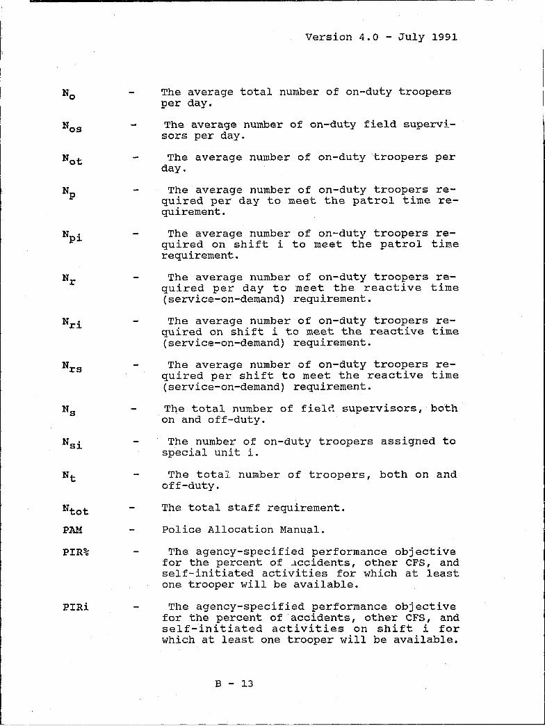
PIR%
PIRi
Version 4.0 - July 1991
The average total number of on-duty troopers per day_
The average number of on-duty field supervisors per day.
The average number of on-duty troopers per day.
The average number of on-duty troopers required per day to meet the patrol time requirement.
The average number of on-duty troopers required on shift i to meet the patrol time requirement.
The average number of on-duty troopers required per day to meet the reactive time (service-on-demand) requirement.
The average number of on-duty troopers required on shift i to meet the reactive time (service-an-demand) requir~ment.
The average number of on-duty troopers required per shift to meet the reactive time (service-an-demand) requirement.
The total number of fiel~ supervisors, both on and off-duty.
The number of on-duty troopers assigned to special unit i.
The total number of troopers, both on and off-duty.
The total staff requirement.
Police Allocation Manual.
The agency-specified performance objective for the percent of ~ccidents, other CFS, and self-initiated activities for which at least one trooper will be available.
The agency-specified performance objective for the percent of accidents, other CFS, and self-initiated activities on shift i for which at least one trooper will be available.
B - 13

Version 4.0 - July 1991
SRF
TA
TC
TE
TN
The shift relief factor.
The total staff to be added (or subtracted) for the allocation.
The total current staff.
The total staff requirement based on PAM estimates.
Total overstaffing (or understaffing) based on current staff levels and PAM staff estimates for each APA.
B - 14

Version 4.0 - July 1991
APPENDIX C: Example using PAM Worksheets 1 - 9 To Determine Staffing Requirements and Allocation
Introduction
This appendix illustrates the use of worksheets 1-8 to determine staffing levels for one APA and Worksheet 9 to allocate staff among six APAs. The data used for this example are based on information obtained from the field test agencies during Phase I of the PAM project.
The remainder of this appendix is divided into two parts. The first presents observations about the example agency and the particular options used in each worksheet. Comparisons between the data values used or calculated for the example and the field test results (see Table 1) are also discussed. The second part consists of the completed worksheets.
Observations
In the discussion below, references to specific values in the worksheets are made by identifying the corresponding worksheet step numbers in parentheses.
Worksheet 1: Operations, Workload, and Highway Data
The example APA covers a large geographic area near a major metropolitan center. The state agency has full police powers and handles a large number of accidents (1.3.2) and other calls-forservice (CFS) (1.3.4) per year. The APA contains 52.7 miles of interstate highways (1.4.1) and 191.4 miles of primary highways (1.4.2). The state agency provides full coverage (i.e., 168 hours per week) «1.2.5.1) and (1.2.6.1» and high visibility «1.2.5.3) and (1.2.6.3» on the interstate and primary highways. Coverage and visibility on secondary highways are limited «1.2.7.1) and (1.2.7.3».
Worksheet 2: Administrative Time
The agency uses Section 201 to set administrative time to 9.7 minutes per hour per trooper. The field test average for Section 2.1 was 10.83 minutes.
C - 1

Version 4.0 - July 1991
Wor~9heet 3: Reactive Time
The total obligated time per day for the agency is 57.47 hours (3.3.1) which consists of 39.6 hours for accidents (3.1.5) and 17.87 hours for all other CFS (3.2.5). Based on an 3-hour shift, this level of workload requires 7.18 on-duty troopers per day (3.3.3). The average service time for accidents is 3.82 hours (3.1. 2) which is slightly higher than the field test av/~rage of 3.10 hours. The average time of 0.90 hours for all other CFS (3.2.2) is considerably lower than the field test average of 1.66 hours.
Worksheet 4: Proactive Time - Self-Initiated
The agency determines the self-initiated time based on the historical experience of the agency in section 4.3. The average of 8.97 minutes per hour per trooper is slightly lower than the field test average of 11.57 minutes for the same section.
Worksheet 5: Proactive Time - Patrol
In section 5. 1, 'the agency determines a total requirement of 10.91 on-duty troopers per day (5.l.S) to provide the desired level of patrol visibility. The 10.91 troopers consist of 3.16 troopers (5.1.2.5) for controlled-access highways to meet a 1-hour patrol interval objective (5.1.2.4) and 7.18 troopers (5.1.3.5) on primary highways to meet a 2-hour patrol interval goal (5.1.3.4). Only 0.57 on-duty troopers per day are needed for the secondary highways (5.1.4.5) because of limited coverage (5.1.4.2) and low visibility (5.1.4.4».
For patrol availability, the agency examines two options: the immediate response option in Section 5.2 and the t::r'avel time for line patrol option in section 5.4. Based on an immediate response objective of 95% (5.2.6), the agency determines that 4.2 on-duty troopers (5.2.7) are needed per shift to insure that at least one trooper will be available for 95% of the accidents, other CFS, and self-initiated activities when they occur. The daily requirement for 3 shifts is 12.6 troopers (5.2.8).
The assumptions implied with the use of section 5.2 are that ma equals 9 minutes, ms equals 15 minutes, and that staffing is equal over all shifts. For the example, the actual values are ms = 9.7 minutes (2.3), ms = 8.97 minutes (4.4), and staffing over the 3 shifts is approxlmately 20, 40, and 40 %. If the Supplemental Worksheet in Appendix F (not shown) is used, the total number of on-duty troopers per day is 12.6 which is the same number derived in section 5.2. The adjustment factor (Kf ) in the Supplemental Worksheet, based on ma = 9.7 and ms = 8.97, equals 0.22 which is very close to the Kf = 0.25 value used for Table 3-1.
C - 2

Version 4.0 - July 1991
In Section 5.4, the required on-duty staffing for line patrol operations is determined. The agency operates line patrol units 128 hours a week (5.4.2) over 97.3 highway miles (5.4.3). This provides coverage over all of the interstate and selected primary highways in the jurisdiction during high accident periods. Based on the shift length (5.4.1), response speed (5.4.4), and travel time objective of 12 minutes, a total of 8.24 on-duty troopers (5.4.6) are needed.
To determine the number of troopers for availability, the agency compares the results of sections 5.2 and 5.4 and selects the larger value (i.e., 12.6 on-duty troopers for immediate response, Section 5.2) The last step in Worksheet 5 (5.6) is to determine the number of on-duty troopers for patrol. This is done by comparing the number of on-duty troopers needed for "visibility" (i.e, 10.91 troopers in Step 5.1.5) with the number of troopers needed for "availability" (i.e., 12.6 troopers in Step 5.5) and selecting the larger value. Hence, a value of 12.6 troopers is entered in Step 5.6.
Worksheet 6: Average Daily Number of On-Duty Troopers
The agency uses section 6.1 to determine that 28.72 on-duty troopers (6.1.5) will be needed each day. Since some patrol units are staffed with two troopers for evening patrols (estimated to be about 25% of the patrols (6.2.1», the number of troopers is increased to 35.89 (6.2.4). section 6.3 is not used since no minimum staffing requirements are used in the APA.
Worksheet 7: Special Assignment and Field Supervision
Worksheet 7 is used to adjust the number of troopers for patrol work performed by field supervisors and troopers on special assignment. For the example agency, each field supervisor is responsible for an average of 7 troopers and spends approximately 25% of his/her time on patrol (i.e., non-supervisory) activities. In section 7.1, the agency determines that the adjusted number of on-duty, fulL-time troopers is 34.67 (7.1.6).
The agency has an average of 6 troopers (7.2.1.2) on-duty each day for commercial vehicle enforcement. Each trooper assigned to the unit spends about 40% of his/her time on patrol (7.2.1.3). The adjusted number of on-duty troopers for commercial vehicle enforcement is 3.48 (7.2.1.6).
The total adjusted daily number of on-duty troopers equals 38.15 (7.2.4). The number of on-duty, full-time troopers can be obtained by subtracting all of the on-duty special assignment staff (i.e, 6 troopers in the example) from the total adjusted number of troopers found in S'tep 7.2.4; that is, the number of on-duty, full-time troopers equal 32.15.
C - 3

Version 4.0 - July 1991
The -total number of on--duty field supervisors required per day is 5.45 (7.3.1). This value is obtained by dividing the adjusted number of on-duty troopers (7.2.4) by the average number of troopers that report to each supervisor (7.1.1).
Worksheet 8: Total Staff Requirement
Based on the average number of on-duty hours spent on patrol per year (8.2.3), the shift relief factor for the agency is 1.716 (8.2.4). Multiplying the on<oduty trooper and field supervisor estimates by the shift relief factor yields the total staff requirements (i.e., 65.47 troopers (8.3.1) and 9.35 field supervisors ( 8 . 3 . 2) ) •
The agency uses section 8.4 to specify a total of 5 staff and command personnel. The total staff requirement of 79.82 officers for the APA is de-termined in section 8.7.
Worksheet 9: Allocation of Patrol Personnel Among Several APAs
Only Table 4-1 from Worksheet 9 is shown below to illustrate the allocation procedure. The allocation example is based on 6 APAs. The current staffing levels for each APA are shown in column 1. The sum of column 1 indicates that the total current staffing (TC) is 382 troopers. The PAM staffing estimates for each APA are shown in column 2. (APA 1 is the example used for worksheets 1-8.) The sum of column 2 indicates that the total staff estimate (TE) for the 6 APAs from the PAM model is 412.52 troopers. Comparison of the columns 1 and 2 indicates that all of the APAs are understaffed except APA 2. For the example allocation, 20 additional troopers (TA) are to be added to the current staffing total of 382 troopers.
The values for the unconstrained allocation of the 402 troopers (i.e., 382 + 20) are shown in column 3. (See step 9.1.7 in Worksheet 9 for the formula used to determine the values in column 3.) Note that the allocation shown in column 3 could only be achieved by reassigning some of the current staff (e.g., some troopers would have be taken from APA 2).
Columns 4 - 8 are used to determine the constrained allocation of the 402 troopers. The difference between the values in columns 1 and 3 for each AP'A are shown in column 4. The difference indicates the amount of over or understaffing for each APA. (Only APA 2 has a positive value which indicates it is overstaffed.) Since the total staff is to be increased (i.e., TA > 0), the procedures described in step 9.2.3 are used to determine the values in column 5. (For each APA, if a column 4 value is negative, it is copied in column 5. If a column 4 value is positive, a zero is entered in column 5.) step 9.2.3.3 is used to calculate how the 20 new troopers will be distributed over the 6
C - 4

Version 4.0 - July 1991
APAs (column 6). For the constrained allocation procedure, staff is only added to APAs that are understaffed (i.e, APAs that have negative values in column 5). The values in column 6 are rounded to whole numbers and entered column 7. (The sum of the values in column 7 must equal the number of staff to be added; that is, column 7 must sum to 20.) The final value for each APA for the constrained allocation, shown in column 8 t is obtained by adding the current staff (column 1) to the staff to be added (column 7).
C - 5

Version 4.0 - July 1991
WORKSHEET 1: Operations, Workload, and Highway Data
Objective: Identify data items to be used for determining the number of state-wide traffic services personnel within an APA.
Method: Data is identified as either operations, workload, or highway.
1.1 Autonomous Patrol Area Name 1 Detailed Example
(1.1)
============================= .. -
1.2 Operations Data for the APA
1.2.1 Shift length (hours) ••.•...
1.2.2 Average number of on-duty hours per year per trooper
1.2.3 Average number of troopers to be supervised by each field supervisor • . . . .
1.2.4 Percentage of field supervisor on-duty time spent on patrol, reactive, and self-initiated activities . . . . . . . . . .
C - 6
8.0
(1.2.1)
1,702.0
(1.2.2)
7.0
(1.2.3)
25.0
(1.2.4)

Version 4.0 - July 1991
1.2.5 Patrol operations - controlled-access highways
1.2.5.1 Coverage per week (hours), (maximum value = 168) . • •
1.2.5.2 Average patrol speed (MPH) • • • • • • • •
1.2.5.3 Patrol interval performance objective (hours) • . • • • • .
1·2.6 Patrol operations - primary highways
1.2.6.1 Coverage per week (hours), (maximum value = 168) • • •
1.2.6.2 Average patrol speed (MPH) • • • • • • • •
1.2.6.3 Patrol interval performance objective (hours) • . • • . • •
1.2.7 Patrol operations - secondary highways
1.2.7.1 Coverage per week (hours) (maximum value = 168) • .
1.2.7.2 Average patrol speed (MPH) • • • • • • • •
1.2.7.3 Patrol interval performance objective (hours) . . . . . . .
C - 7
168.0 .J (1.2.5.1)
50.0
(1.2.5.2)
1.0
(1.2.5.3)
168.0
(1.2.6.1)
40.0
(1.2.6.2)
2.0
(1.2.6.3)
128.0
(1.2.7.1)
30.0
(1.2.7,,2)
168.0 ] (1.2.7.3)

Version 4.0 - July 1991
1.3 Workload Data for the APA
1.3.1 Total number of days in the sample period • . .
1.3.2 Total number of accidents handled by state the agency during the sample period • •
1.3.3 Average service time (hours) per accident • • • • • • • •
1.3.4 Total number of other CFS handled by the state agency during the sample peri~)d . •
1.3.5 Average service time (hours) per CFS ••. . • . • • • •
1.4 Highway Data for the APA
1.4.1 Controlled-access highways (miles) .•••.••..
1.4.2 ~rimary highways (miles) •••••
1.4.3 Secondary highways (miles) ••••
C - 8
365.0
(1.3.1)
3,784.0
(1.3.2)
3.82~ (1.3.3)
7,249.0
(1.3.4)
0.90
(1.3.5)
52.7
(1.4.1)
191.~
(1.4.2)
1,265.1
(1.4.3)

version 4.0 - July 1991
WORKSHEET 2: Administrativo Time
objective: Determine the average number of minutes per hour per trooper to be spent on administrative activities within the APA (rna)'
Method: Based either on policy decision or historical experience.
OPTION: Complete section 2.1 ~ Section 2.2.
2.1 Average Number of Minutes Per Hour Per Trooper - Policy Deoision
Select administrative time performance objective in minutes per hour per trooper . . . . . .
continue with section 2.3.
OR
r~ 9.7 L._
(2.1)
2.2 Average Number of Minutes Per Hour Per Trooper -Historioa1 Experience
2.2.1 Total time (hours) spent on administrative activities within the APA during the sample period
2.2.2 Total on-duty hours by patrol troopers within the APA during the sample period . . . . . . . .
c - 9
(2.2.1)
(2.2.2)
~------------------- ------------------------------------ --------------- --

version 4.0 - July 1991
2.2.3 Fraction of time spent on administrative activities, divide: (2.2.1) + (2.2.2)
(2.2.3)
2.2.4 Average number of minutes per l hour per trooper, multiply: _ (2.2.3) x 60 • • • • • • . . • ~--------~
2.3 Administrative Time
Minutes per hour per trooper, select either (2.1) or (2.2.4) (note: 0 ~ rna < 60 )
C - 10
(2.2.4)
Ik=II =9=.7===:!.J11 (rna)
(2.3)

Version 4.0 - July 1991
WORKSHEET 3: Reactive Time
Objective: Determine the number of troopers required to handle accidents and other CFS within an APA (Nr ).
Method: Based on the total time required to handle all accidents and other CFS, and the shift length.
3.1 Daily Service Time Requirement for Accidents
3.1.1 Total number of accidents within the APA during the sample period, use (1.3.2)
3.1.2 Average service time (hours) for each accident, use (1.3.3)
3.1.3 Total obligated time for accidents within the APA during the sample period, mul tiply: (3. 1. 1) x (3. 1. 2) (or enter directly from CAD system)
3.1.4 Total number of days in the sample period, use (1.3.1) .
3.1.5 Average workload per day for accidents (hours), divide: (3.1.3) + (3.1.4) ..•
C - 11
3,784.0
(3.1.1)
3.82
(3.1.2)
14,454888
(3.1.3)
365.0
(3.1.4)
39.6
(3.1.5)

----------------------------------------------------------------------------
Version 4.0 - July 1991
3.2 Daily service Time Requirement for Other CFS
3.2.1 Total number of other CFS within the APA during the 7,249.0 sample period, use (1.3.4) · · · · (3.2.1)
I 3.2.2 Average service time (hours) 0.90 fc)r each CFS, use (1.3.5) · · · · (3.2.2)
3.2.3 Total obligated time for other CFS within the APA during the sample period, 6,524.1 multiply: (3.2.1) x (3.2.2) · · · (or enter directly from CAD system) (3.2.3)
3.2.4 Total number of days in the 365.0 ] sample period, use (1.3.1) · · · · (3.2.4)
3.2.5 Average workload per day for other CFS (hours), divide: 17 .. 87 (3.2.3) . (3.2.4) . . . . · · · · (3.2.5)
3.3 Total Number of Troopers Required per Day for R4~acti ve Time
3.3.1 Total average workload per L57.47 day within the APA (hours),
add: (3.1.5) + (3.2.5) . . .. (3.3.1)
[ 3.3.2 Shift length (hours), 8.0 l use (1.2.1) . . . . . · · · · (3.3.2)
3.3.3 Average number of on-duty troopers required per day within the APA to meet the
II II average daily workload, 7.18 (Nr ) divide: (3.3.1) (3.3.2) . . . . .
(3.3.3)
C - 12

version 4.0 - July 1991
WORKSHEET 4: Proactive Time - Self-initiated
Objective: Determine the average number of minutes per hour per trooper to be spent on self-initiated activities within the APA (ms ).
Method: Based either ~n policy decision or historical experience within the APA.
OPTION: Complete section 4.1 or Section 4.2 or Section 4.3.
4.1 Average Number of Minutes Per Hour Per Trooper - Policy Decision (Direct)
Select self-initiated performance objective for the APA, minutes per hour per trooper
continue with Section 4.4
OR
(4.1)
4.2 Average Number of Minutes Per Hour Per Trooper - Policy Decision (Indirect)
4.2.1 Total number of self-initiated contacts within the APA during the sample period . • •
4.2.2 Total time (hours) spent on self-initiated contacts within the APA by all troopers on patrol during the sample period
C - 13
(4.2.1)
(4.2.2)

version 4.0 - July 1991
4.2.3 Average time (hours) per self-initiated contact within the APA during the sample period, divide: (4.2.2) + (4.2.1) •...
4.2.4 Select number of self-initiated contacts per shift per trooper performance objective . . • . • .
4.2.5 Shift length (hours), use (1.2.1) ..•••
4.2.6 Number of self-initiated contacts per hour per trooper, divide: (4.2.4) + (4.2.5)
4.2.7 Self-initiated performance objective for the APA in minutes per hour per trooper, multiply: 60 x (4.2.3) x (4.2.6) ..... .
continue with section 4.4
OR
(4.2.3)
(4.2.4)
(4.2.5)
(4.2.6)
(4.2.7)
4.3 Average Number of Minutes Per Hour Per Trooper -Historical Experience
4.3.1 Total time (hours) spent on self-initiated contacts within the APA by all troopers on patrol during the sample period, (same as (4. 2 . 2) ) ....•.•.
4.3.2 Total on-duty hours by troopers on patrol within the APA during the sample period, (same as (2.2.2» .•...•.•
c - 14
19,821.0
(4.3.1)
[132,614. 16 1
(4.3.2)
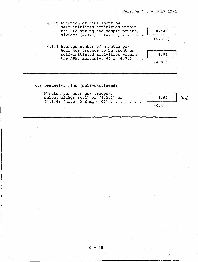
version 4.0 - July 1991
4.3.3 Fraction of time spent on self-initiated activities the APA during the sample divide: (4.3.1) + (4.3.2)
within period,
4.3.4 Average number of minutes per hour per trooper to be spent on self-initiated activities within the APA, multiply: 60 x (4.3.3) .
4.4 Proactive Time (Self-initiated)
0.149
(4.3.3)
8.97
(4.3.4)
Minutes per hour per trooper, I I select either (4.1) or (4.2.7) or 8.97 l (ms) (4.3.4) (note: 0 ~ ms < 60) . . . . . .. ~========~
(4.4)
C - 15

Version 4.0 - July 1991
WORKSHEET 5: Proactive Time - Patrol
Objective: Determine the number of troopers required within the APA to provide an adequate level of visibility and availability.
Method: Based on: (1) the patrol interval, and (2) th~ probability of immediate response to accidents and other CFS or the average tr~vel time to accidents and other CFS.
5.1 Patrol visibility
5.1.1 Shift le-ngth (hours), use (1. 2 ~ 1) •••••
5.1.2 Number of troopers needed per day for patrol on controlled-access highways in the APA
5.1.2.1 Miles of highway, use (1.4.1) ••.
5.1.2.2 Hours of coverage per week, use (1.2.5.1) .
5.1.2.3 Average patrol speed (MPH), use (1.2.5.2)
5.1. 2.4 Performance objective patrol interval (hours), use (1.2.5.3) ••.•••
C - 16
8.0
(5.1.1)
52.7
(5.1.2.1)
[ 168.0
(5.1.2.2)
50.0
(5.1.2.3)
1.0
(5.1.2.4)
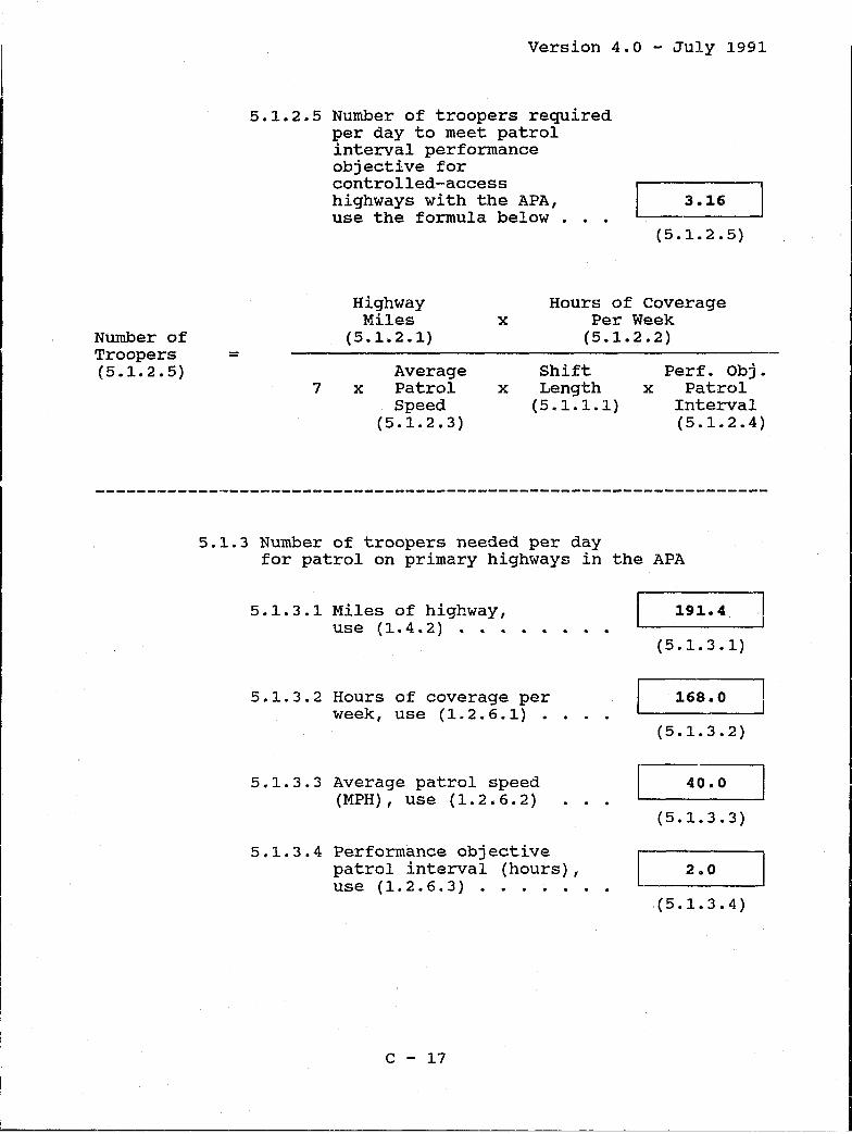
Number of Troopers (5.1.2.5)
=
Version 4.0 - July 1991
5.1.2.5 Number of troopers required per day to meet patrol interval performance objective for controlled-access highways with the APA, 3.16
7
use the formula below •
Highway Miles
(5.1.2.1)
Average x Patrol
Speed (5.1.2.3)
x
(5.1.2.5)
Hours of Coverage Per Week
(5.1.2.2)
Shift x Length
(5.1.1.1.)
Perf. Obj. x Patrol
Interval (5.1.2.4)
5.1.3 Number of troopers needed per day for patrol on primary highways in the APA
5.1.3.1 Miles of highway, use (1.4.2) .••
5.1.3.2 Hours of coverage per week, use (1.2.6.1) .
5.1.3.3 Average patrol speed (MPH), use (1.2.6.2)
5.1.3.4 Performance objective patrol interval (hours), use (1.2.6.3) ..... .
C - 17
191.4
(5.1.3.1)
168.0
(5.1.3.2)
40.0
(5.1.3.3)
2.0
(5.1.3.4)
J

--~--~------------------------------------------------------------------------
Version 4.0 - July 1991
Number of Troopers (5.1.3.5)
=
5.1.3.5 Number of troopers required per day to meet patrol interval performance objective for primary highways within the APA, use the formula below . •
7.18
(5.1.3.5)
Highway Miles
(5.1.3.1) x
Hours of Coverage Per Week
(5.1.3.2)
7 Average
x Patrol Speed
(5.1.3.3)
Shift x Length
(5.1.1.1)
Perf. Obj. x Patrol
Interval (5.1.3.4)
5.1.4 Number of troopers needed per day for patrol on secondary highways in the APA
5.1.4.1 Miles of highway, use (1.4.3) •••
5.1.4.2 Hours of coV'erage per week, use (1.2.7.1) .
5.1.4.3 Average patrol speed (MPH), use (1.2.7.2)
5.1.4.4 Performance objective patrol interval (hours), use (1.2.7.3)
C - 18
1,265.1
(5.1.4.1)
128.0
(5.1.4.2)
(5.1.4.3)
168.0
(5.1.4.4)

Number of Troopers (5.1.4.5)
=
version 4.0 - July 1991
5.1.4.5 Number of troopers required per day to meet patrol interval performance objective for
~I
secondary highways within the APA, use 0.57 the formula below . . • • •
Highway Miles
(5.1.4.1)
Average x Patrol
Speed (5.1.4.3)
x
(5.1.4.5)
Hours of Coverage Per Week
(5.1.4.2)
Shift x Length
(5.1.1.1)
Perf. Obj. x Patrol
Interval (5.1.4.4)
5.1.5 Total nunilier of troopers required per day to meet patrol interval performance objective within the APA, add: (5.1.2.5) + (5.1.3.5) + (5.1.4.5)
[ 10.91 .J (5.1.5)
OPTION: Complete Section 5.2 or section 5.3 ~ Section 5.4 or the Supplemental Worksheet in Appendix F.
5.2 Patrol Availability - Immediate Response
5.2.1 Shift length (hours), use (1,2,1) ..•..
C - 19
8.0
(5.2.1)
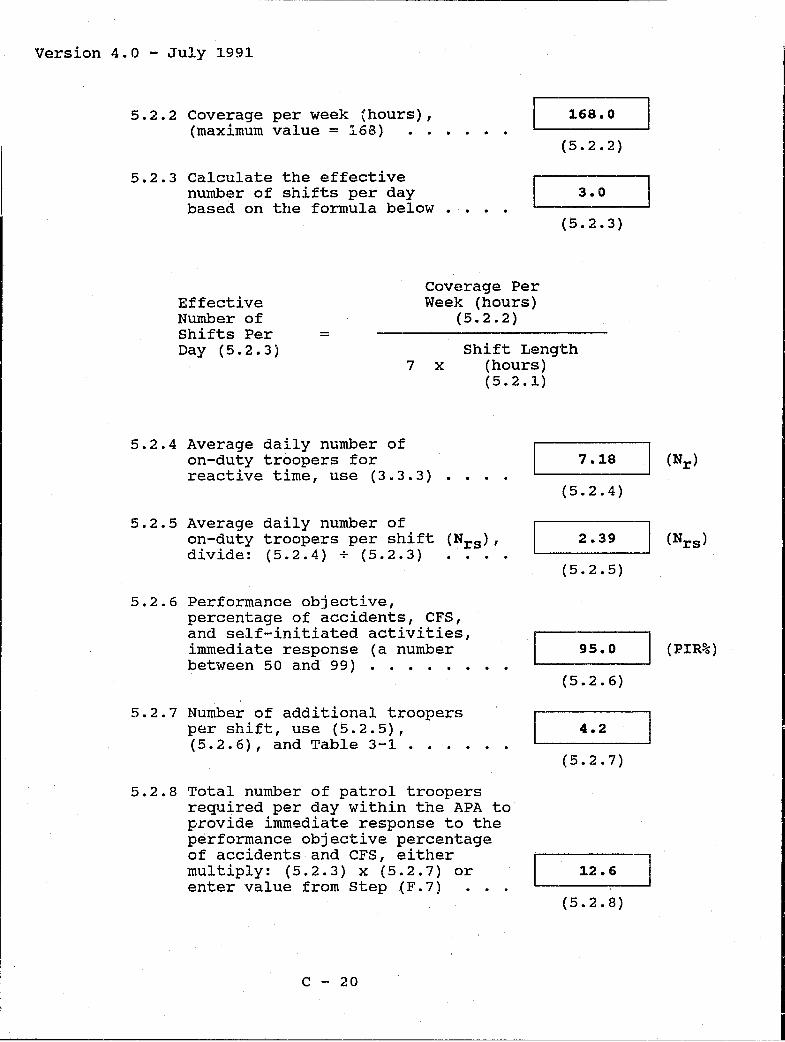
~-----------------------------------------------------------------------
version 4.0 - July 1991
5.2.2 Coverage per week {hours), (maximum value = 168)
5.2.3 Calculate the effective number of shifts per day based on the formula below
=
Coverage Per Week (hours)
(5.2.2)
168.0
(5.2.2)
3.0
(5.2.3)
Effective Number of Shifts Per Day (5.2.3j Shift Length
7 x (hours) (5.2.1)
5.2.4 Average daily number of on-duty troopers for reactive time, use (3.3.3)
5.2.5 Average daily number of on-duty troopers per shift (Nrs )' divide: (5.2.4) . (5.2.3) ....
5.2.6 Performance objective, percentage of accidents, CFS, and self-initiated activities, immediate response (a number between 50 and 99) • • . . . •
5.2.7 Number of additional troopers per shift, use (5.2.5), (5.2.6), and Table 3-1 ...•
5.2.8 Total number of patrol troopers required per day within the APA to ~rovide immediate response to the performance objective percentage of accidents and CFS, either multiply: (5.2.3) x (5.2.7) or enter value from step (F.7) ••.
C - 20
[
7.18
(5.2.4)
2.39
(5.2.5)
95.0 ] (PIR%)
(5.2.6)
4.2
(5.2.7)
12.6
(5.2.8)
_J

Table 3-1
Number of Patrol Troopers Required To Provide Immediate Response Capability Based On the Average Number of Reactive Troopers Required and the Selected Response Percentage (Ks = 0.25)
Number of ----- Performance objective Immediate Response Percentage (PIR%) (5.2.6) -----
Reactive Troopers 50 60 70 75 80 85 90 95 97 98 99 (Nrs ) (5.2.5)
.05 0.3 0.4 0.6 0.8 0.9 1.1 1.4 2.0 2.4 2.7 3.3
.10 0.3 0.5 0.7 0.8 1.0 1.2 1.5 2.1 2.S 2.8 3.4
.15 0.3 0.5 0.8 0.9 1.1 1.3 1.6 2.2 2.6 2.9 3.5 ()
.20 0.4 0.6 0.8 1.0 1.1 1.3 1.7 2.2 2.7 3.0 3.6
.25 0.4 0.6 0.9 1.0 1.2 1.4 1.7 2.3 2.8 3.1 3.7 t\) .30 0.5 0.7 0.9 1.0 1.2 1.5 1.8 2.4 2.8 3.2 3.8 I-'
.40 0.5 0.7 1.0 1.1 1.3 1.6 1.9 2.5 3.0 3.4 4.0
.50 0.6 0.8 1.0 1.2 1.4 1.7 2.0 2.7 3.1 3.5 4.2
.60 0.6 0.8 1.1 1.3 I.!':> 1.7 2.1 2.8 3.3 3.6 4.3
.80 0.6 0.9 1.2 1.4 1.6 1.9 2.3 3.0 3.5 3.9 4.6 1. 00 0.8 1.0 1.3 1.5 1.7 2.0 2.5 3.2 3.7 4.1 4.8 <l
(!) 1. 20 0.8 1.1 1.4 1.6 1.8 2.2 2.6 3.4 3.9 4.3 5.1 Ii rn ..... 1.60 0.9 1.2 1.5 1.8 2.0 2.4 2.9 3.7 4.3 4.7 5.5 0 2.00 1.0 1.3 1.7 1.9 2.2 2.6 3.1 4.0 4.6 5.0 5.9 ::1
2.50 1.1 1.4 1.8 2.1 2.4 2.8 3.4 4.3 4.9 5.4 6.3 ,r:.
0 3.00 1.2 1.5 2.0 2.3 2.6 3.0 3.6 4.6 5.2 5.8 6.7 4.00 1.3 1.7 2.2 2.5 2.9 3.4 4.0 5.1 5.8 6.4 7.4 I
5.00 1.5 1.9 2.4 2.8 3.2 3.7 4.4 5.5 6.3 6.9 8.0 C-j C r-'
"< I-' \0 \0 I-'
................ ~ ............................ --...... ------.. ----------------~------------------------~-----------------------------------------------------------------------------------------

Version 4.0 - July 1991
continue with section 5.5.
OR
5.3 Patrol Availability - Travel Time for Are~ Patrol
5.3.1 Shift length (hours), use (1,2,1) •..••
5.3.2 Coverage per week (hours) (maximum value = 168)
5.3.3 Area (square miles) of the APA . . . . • . • • .
5.3.4 Average response speed (MPH) (equal to or greater than average patrol speed) •••
5.3.5 Average travel time performance objective (minutes) ...••.•
5.3.6 Number of troopers requi~ed within the APA to meet the av(~rage travel time performance objective
5.3.6.1 Calculate K based on formula below • •
(5.3.1)
(5.3.2)
(5.3.3)
(5.3.4)
(5.3.5)
(5.3.6.1)
K = Speed (MPH)
(5.3.4)
C - 22
40
x Time (min) (5.3.5)
(K)

version 4.0 - July 1991
=
5.3.6.2 Calculate K x K, multiply (5.3.6.1) x (5.3.6.1) .•.
5.3.6.3 Number of troopers required, use the formula below • . •
K2 (5.3.6.2)
x Area (5.3.3)
x
(5.3.6.2)
(5.3.6.3)
coverage Per Week (Hours)
(5.3.2) No. of on-Duty
Troopers, Area Patrol
(5.3.6.3) 7 x Shift Length
(hours) (5.3.1)
continue with Section 5.5.
OR
5.4 Patrol Availability - Travel Time for Line Patrol
5.4.1 Shift l~~gth (hours), use ( 1 , 2 , 1) •.... . . . . . . 8.0
(5.4.1)
]
5.4.2 Coverage per week (hours), (maximum value = 168) • :9 • .,
128.0 ~ (5.4.2)
5.4.3 Total highway miles to be patrolled within the APA .
c - 23
• • • f
97.30
(5.4.3)
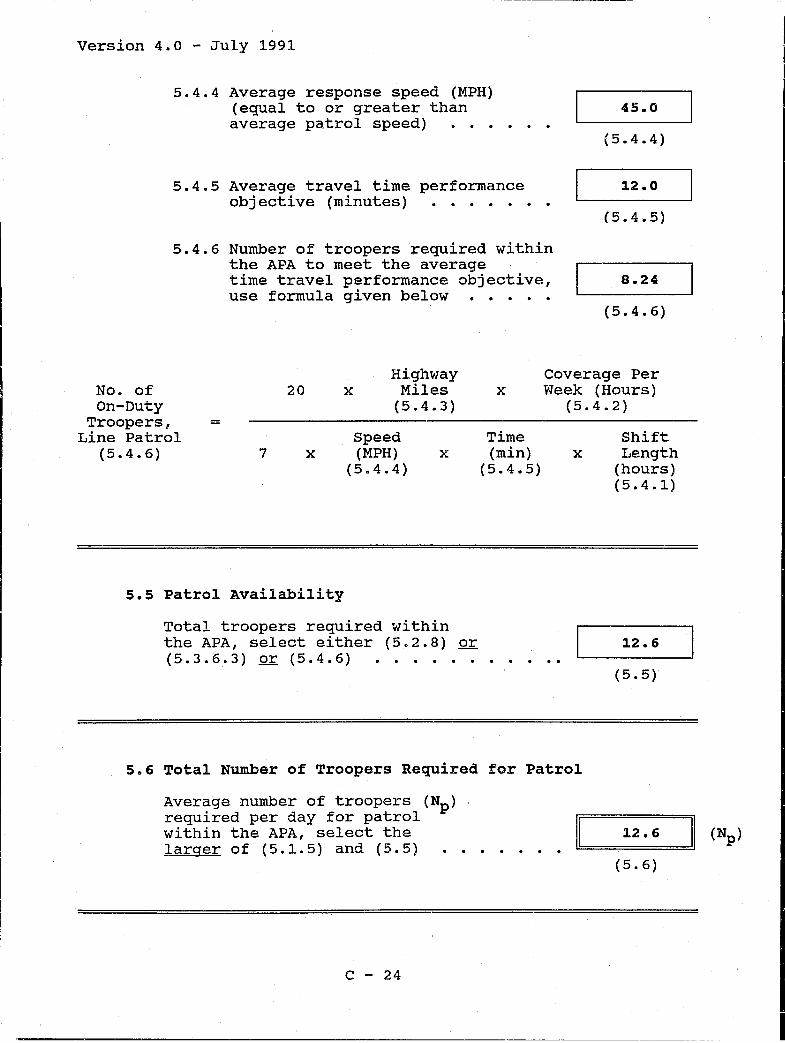
Version 4.0 - July 1991
5.4.4 Average response speed (MPH) (equal to or greater than average patrol speed) •..
5.4.5 Average travel time performance objective (minutes) ..•..•.
5.4.6 Number of troopers required within the APA to meet the average time travel performance objective, use formula given below . . . . .
45.0
(5.4.4)
12.0
(5.4.5)
8.24
(5.4.6)
No. of On-Duty
Troopers, Line Patrol
(5.4.6)
20 Highway
x Miles (5.4.3)
x Coverage Per Week (Hours)
(5.4.2) =
Speed 7 x (MPH) x
(5.4.4)
5.5 Patrol Availability
Total troopers required within the APA, select either (5.2.8) or ( 5 • 3 • 6 • 3 ) or ( 5 • 4 • 6) ••••••
Time (min)
(5.4.5)
Shift x Length
(hours) (5.4.1)
12.6
(5.5)
5.6 Total Number of Troopers Required for Patrol
Average number of troopers (Np ) required per day for patrol within the APA, select the larger of (5.1.5) and (5.5)
C - 24
. . . . . l!:::::11 =12=. 6====:!J11 (Np )
(5.6)
I

Version 4.0 - July 1991
WORKSHEET 6: Average Daily Number of On-Duty Troopers
Ob'jective: Determine the average total number of troopers required per day within the APA.
Method: Combine the total number of troopers required for reactive (Nr > and patrol activities (Ng ) with the per trooper time requirements for selr-initiated (ms) and administrative (ma ) activities. Adjust the required number of troopers based on the percentage of two-trooper patrols and, if applicable, minimum daily staffing levels.
6.1 Number of on-Duty Troopers per Day - All One-Trooper Patrols
6.1.1 Administrative time - minutes per hour per trooper, use (2.3) •••••.•••.
6.1.2 Average number of troopers required per day to meet reactive time workload, use (3. 3 • 3 ) ..••••••...
6.1.3 Self-initiated time - minutes per hour per trooper, use (4.4) •.•.••....
6.1.4 Average number of troopers required per day to meet patrol time requirements, use (5.6) .•
6.1.5 Average total number of on-duty troopers required per day for all patrol activities within the APA, one trooper per unit, use the formula below . • . . • •
C - 25
9.7
(6.1.1)
7.18
(6.1.2)
8.97
(6.1.3)
(6.1.4)
28.72
(6.1.5)

version 4.0 ~ July 1991
Average Total Number of On-Duty Troopers Per Day (6.1. 5)
=
1
Nr (6.1.2) +
ma (6.1.1)
60
Np (6.1. 4)
ms (6.1. 3)
60
===="========================================================
6.2 Adjustment for Two~Trooper Patrols
NOTE: If two-trooper patrols are not used, enter (6.1.5) into (6.2.4) and continue with section 6.3.
6.2.1 Percentage of time patrol units within the APA are staffed with two troopers
6.2.2 Fraction of time patrol units within the APA are staffed with two troopers, divide: (6.2.1) + 100
6.2.3 Adjustment factor: average number of troopers per unit, add: 1 + (6.2.2) •..•••
6.2.4 Average total number of on-duty
25.0
(6.2.1)
0.25
(6.2.2)
1.25
(6.2.3)
troopers required per day for all r---patrol activities, multiply: ~35.89 (6.1.5) x (6.2.3) •.•....•. '-------'
(6.2.4)
C - 26

Version 4.0 - July 1991
6.3 Adjustment for Minimum staffing Levels
Note: If mlnlmum staffing levels are not used, enter (6.2.4) into (6.3.2) and continue with Worksheet 7.
6.3.1 Average minimum number of on-duty troopers required per day for all patrol activities, based on agency policy . • . • • • • • • •
6.3.2 Average daily number of on-duty troopers required for all patrol activities (No)' select the larger of (6.2.4) and (6.3.1)
C - 27
-.;..-(6.3.1)
35.89
(6.3.2)
I

version 4.0 - July 1991
WORKSHEET 7: Special Assignments and Field Supervision
Objective: Determine the additional on-duty personnel required per day because of special assignments and field supervision.
Method: The number of troopers for special assignments is based on the number of specialists assigned by the agency and the percentage of time each spends on field patrol activities. The number of field supervisors is based on the span of supervision (set by agency policy) and the percentage of field supervisor on-duty time spent on patrol activities.
7.1 Number of On-Duty Troopers Required per Day, Adjusted for Field supervisors
7.1.1 Average number of troopers to be supervised by each field supervisor, use (1. 2 • 3) • • •
7.1.2 Percentage of field supervisor on-duty time spent on patrol activities (a number between a and 100), use (1.2.4) ...•..
7.1.3 Fraction of field supervisor on-duty time spent on patrol activities, divide:
7.1. 4
(7.1.2) + 100 ...... .
Total number of on-duty troopers required per day within the APA (N ) for all patrol activi~ies, use (6.3.2)
C - 28
7.00
(7.1.1)
25.00
(7.1.2)
0.25
(7.1.3)
35.89
(7.1.4)

Version 4.0 - July 1991
7.1.5 Adjustment factor (Rf ), use formula below . . .
Adjustment Factor (Rf)
(7.1.5) =
Troopers Per Sgt. (7.1.1)
Troopers Per Sgt. (7.1.1)
0.966
(7.1.5)
Fraction of + Sgt. Time on
Patrol (7.1.3)
7.1.6 Adjusted daily number of full-time, an-duty troopers (Nao ) required per day, use formula below .•.
[[1:==34=. 6=7 ====::!.III (N ao)
Adjusted Number of Full-Time, On-Duty Troopers Per Day
(Nao ) (7.1.6) = x
(7.1.6)
No. of On-Duty Troopers Per Da.y
(No) (7.1.4)
NOTE: If no special assignment personnel are to be included, enter (7.1.6) into (7.2.4) and continue with section 7.3. If special assignment personnel are to be included, continue with section 7.2.
7.2 Number of On-Duty Troopers Required Per Day, Adjusted for special Assignment Personnel
7.2.1 special Assignment 1
7.2.1.1 Assign. 1 name
C - 29
Icommercial Vehicle Ent.
(7.2.1.1)
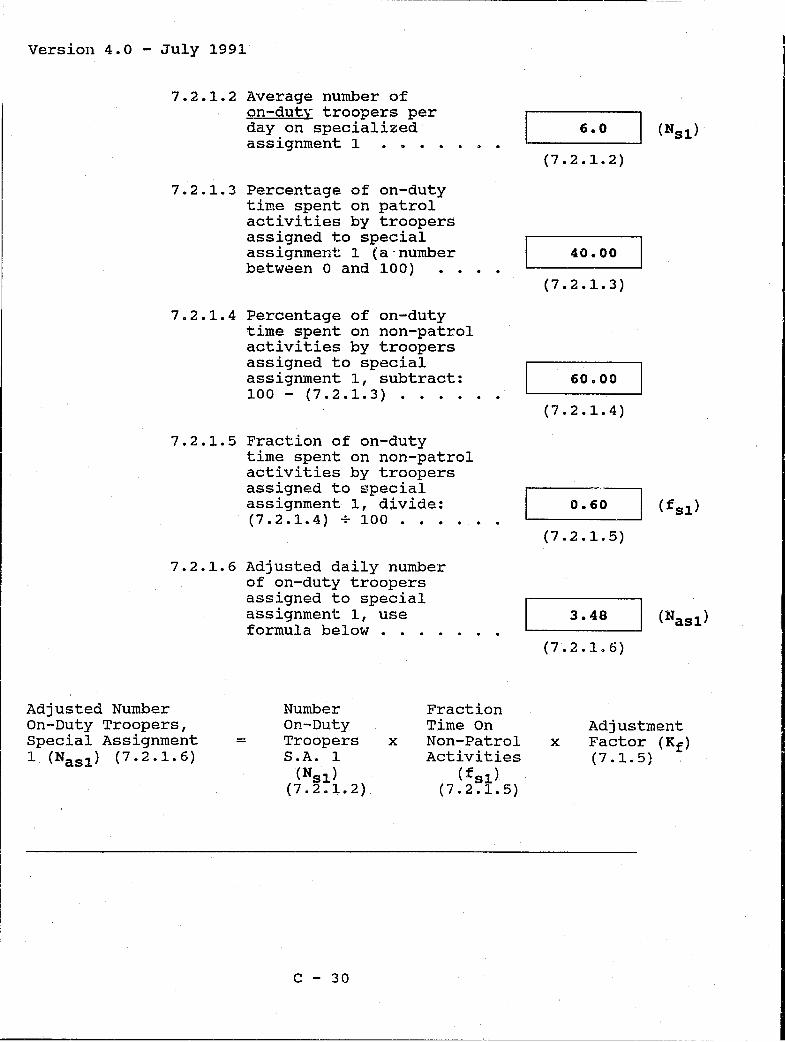
version 4.0 - July 1991
7.2.1.2 Average number of on-duty troopers per day on specialized assignment 1 . · · · · · ·
7.2.1.3 Percentage of on-duty time spent on patrol activities by troopers assigned to special assignment 1 (a "number between 0 and 100)
7.2.1.4 Percentage of on-duty time spent on non-patrol activities by troopers assigned to special assignment 1, subtract: 100 - (7.2.1.3) · ·
7.2.1.5 Fraction of on-duty time spent on non-patrol activities by troopers assigned to special assignment 1, divide: (7.2.1.4) 100 · · · · · ·
7.2.1.6 Adjusted daily number
Adjusted Number On-Duty Troopers, Special Assignment 1 (Nas1 ) (7.2.1.6)
=
of on-duty troopers assigned to special assignment 1, use formula below .
Number On-Duty Troopers x S.A. 1
(Ns1 ) (7.2.1.2)
C - 30
· · · · · ·
Fraction Time On Non-Patrol Activities
(fS1 ) (7.2.1.5)
6.0 (Ns1 )
(7.2.1.2)
40.00
(7.2.1.3)
60.00
(7.2.1.4)
O.6~ I (fS1 )
(7.2.1.5)
3.48 (Nas1 )
(7.2.1.6)
x Adjustment Factor (Rf ) (7.1.5)
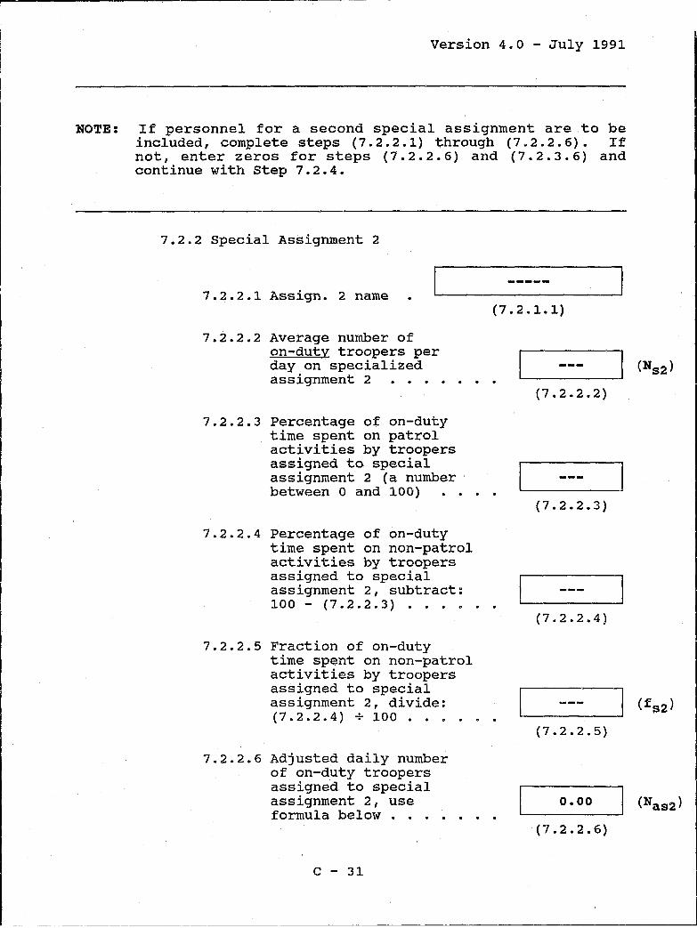
I~------------------~--
version 4.0 - July 1991
NOTE: If personnel for a second special assignment are to be included, complete steps (7.2.2.1) through (7.2.2.6). If not, enter zeros for steps (7.2.2.6) and (7.2.3.6) and continue with step 7.2.4.
7.2.2 special Assignment 2
7.2.2.1 Assign. 2 name (7.2.1.1)
7.2.2.2 Average number of on-duty troopers per day on specialized assignment 2 ...•
7.2.2.3 Percentage of on-duty time spent on patrol activities by troopers assigned to special assignment 2 (a number between 0 and 100)
7.2.2.4 Percentage of on-duty time spent on non-patrol activities by troopers assigned to special assignment 2, subtract: 100 - (7.2.2.3) ..
7.2.2.5 Fraction of on-duty time spent on non-patrol activities by troopers assigned to special assignment 2, divide: (7.2.2.4) + 100 •.....
7.2.2.6 Adjusted daily number of on-duty troopers assigned to special assignment 2, use formula below • . • . . . .
C - 31
~--- -------------~---~---------
_______ --'J (Ns2 )
(7.2.2.2)
(7.2.2.3)
(7.2.2.4)
(7.2.2.5)
0.00
(7.2.2.6)
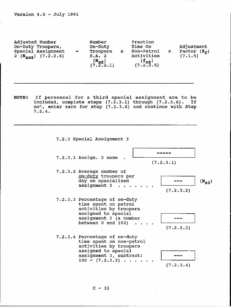
Version 4.0 - July 1991
Adjusted Number On-Duty Troopers, Special Assignment 2 (NaS2 ) (7.2.2.6)
=
Number On-Duty Troopers x S.A. 2
(NS2 ) (7.2.2.::')
Fraction Time On Non-Patrol Activities
(fs2 ) (7.2.2.5)
x Adjustment Factor (Rf ) (7.1.5)
NOTE: If personnel for a third special assignment are to be included, complete steps (7.2.3.1) through (7.2.3.6). If no-!-., en·cer zero for step (7.2.3.6) and continue with step 7.2.4.
7.2.3 Special Assignment 3
7.2.3.1 Assign. 3 name
7.2.3.2 Average number of on-duty troopers per day on specialized assignment 3 . . • •
7.2.3.3 Percentage of on-duty time spent on patrol activities by troopers assigned to special assignment 3 (a number between 0 and 100)
7.2.3.4 Percentage of on-duty time spent on non-patrol activities by troopers assigned to special assignment 3, subtract: 100 - (7.2.3.3) ••.•
C - 32
(7.2.3.1)
(7.2.3.2)
(7.2.3.3)
(7.2.3.4)
J

------------l Version 4.0 - July 1991
7.2.3.5 Fraction of on-duty time spent on non-patrol activities by troopers assigned to special assignment 3, divide: (7.2.3.4) + 100 ••.•.•
7.2.3.6 Adjusted daily number of on-duty troopers assigned to special assignment 3, use
Adjusted Number On-Duty Troopers, Special Assignment 3 (Nas3) (7.2.3.6)
=
formula below . • • • • • •
Number On-Duty Troopers x S.A. 3
(NS3 ) (7.2.3.2)
Fraction Time On Non-Patrol lI .. cti vi ti,es
(fS3) (7.2.3.5)
7.2.4 Adjusted total daily number of on-duty troopers required per day, use formula below •••.
(7.2.3.5)
'--__ o_,,_o_o_~] (Nas3)
II
(7.2.3.6)
x Adjustment Factor (Xf ) (7.1.5)
38.15 II (Not)
(7.2.4)
Adjusted Total Number of On-Duty
Troopers Per Day (Not)
(7.2.4)
= Nao + Nas1 + Nas2 + Nas3 (7.1.6) (7.2.1.6) (7.2.2.6) (7.2.3.6)
C - 33
I
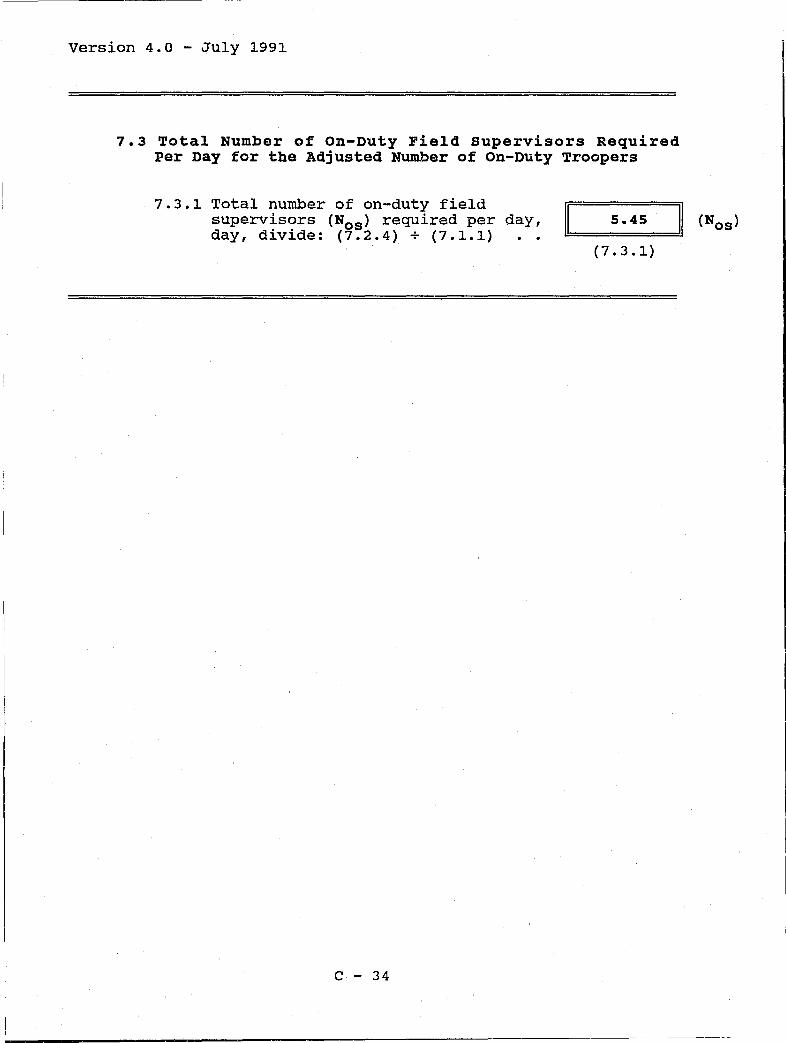
version 4.0 - July 1991
7.3 Total Number of On-Duty Field supervisors Required Per Day for the Adjusted Number of on-Duty Troopers
7.3.1 Total number of on-duty field /1 I superv~sc:>rs (Nos) required per day, I 5.45 I (Nos) day, d1v1de: (7.2.4) + (7.1.1) ~========~
(7.3.1)
C - 34
J

-------,-------------~
Version 4.0 - July 1991
WORKSHEET B: Total Staff Requirements
objective: Determine total staff needed to support the required daily on-duty field personnel.
Method: Use the shift relief factor, daily on-duty staff requirements, and the number of staff and command positions based on either historical data or agency policy.
8$1 On-Duty Troopers and Field Supervisors Required per Day
B.1.1 Total number of on-duty troopers per day within the APA, use (7.2.4) •.•..•.
B.1.2 Total number of on-duty field supervisors per day within the APA, use (7.3.1) ••..•
8.2 Shift Relief Factor
B.2.1 Shift length (hours), use (1.2.1) ....•
B.2.2 Total hours on one shift during one year, multiply: 365 x (B.2.1) •..•.•
C - 35
38.14
(B.1.1)
[ 5.45
(B.1.2)
8.C
(B.2.1)
2,920.0
(B.2.2)
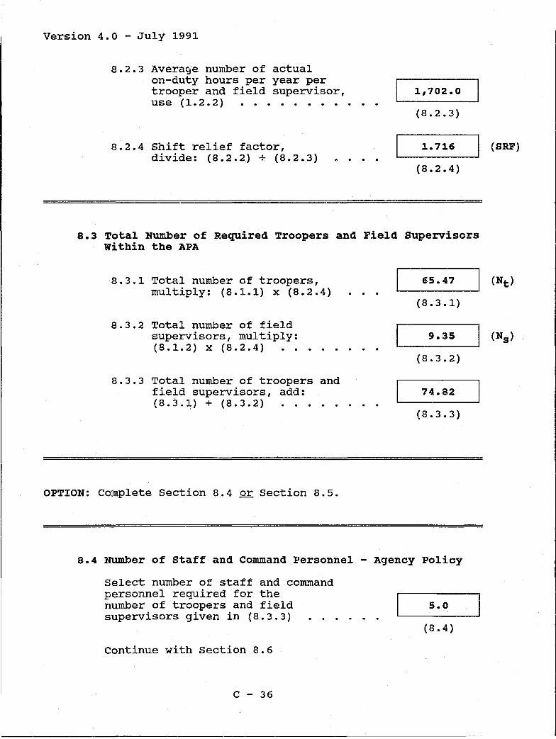
version 4.0 - July 1991
B.2.3 Avera~e number of actual on-duty hours per year per trooper and field supervisor, use (1.2.2) •.••.•••.
B.2.4 Shift relief factor, divide: (B.2.2) + (B.2.3) . . . .
1,702.0
(B.2.3)
1.716
(B.2.4)
8.3 Total Number of Required Troopers and Field supervisors within the APA
B.3.1 Total number of troopers, 65 .. 47 multiply: (B.1.1) x (B.2.4) · · · (B.3.1)
B.3.2 Total number of field supervisors, multiply: 9.35 (B.1.2) x (B.2.4) . . . · · · (B.3.2)
B.3.3 Total number of troopers and field supervisors, add: 74.82 (B.3.1) + (B.3.2) . . . · · · (B.3.3)
OPTION: co:mplete Section B. 4 or Section B. 5.
8.4 Number of staff and Command Personnel - Agency policy
Select number of staff and command personnel required for the number of troopers and field 5.0 supervisors given in (B.3.3) ..... .
(B.4)
Continue with section B.6
C - 36
(SRF)

version 4.0 - July 1991
OR
8.5 Number of staff and Command Personnel - Historical Experience
8.5.1 Current number of troopers and field supervisors within the APA
8.5.2 Current number of staff and command personnel within the APA . • . • •
8.5.3 Average number of staff and command personnel for each trooper and field supervisor, divide: (8.5.2) . (8.5.1)
8.5.4 Required number of troopers and field supervisors within the APA, use (8.3.3) ••
8.5.5 Required number of staff and command personnel within the APA, multiply: (8.5.4) x (8.5.3) .•.•
(8.5.1)
(8.5.2)
(8.5.3)
(8.5.4)
(8.5.5)
8.6 Total Number of Staff and Command Personnel for the APA
Select either (8.4) or (8.5~5) (8.6)
C - 37

Version 4.0 - July 1991
8.7 Total Staff Requirements for the APA
B.7.1 Number of troopers within the APA, use (B.3.1)
B.7.2 Number of field supervisors within the APA, use (B.3.2)
B.7.3 Number of staff and command personnel within the APA, use (B.6)
B.7.4 Total required staff for the APA, add: (B.7.1) + (B.7.2) + (B.7.3)
C - 3B
65.47 (Nt)
(B.7.1)
9.35 1
(Ns )
(B.7.2)
5.00 (Nh )
(B.7.3)
II.!:=:I =7=9.=8=2 ==:::!.III (Ntot>
(8.7.4)

Version 4.0 - July 1991
WORKSHEET 9: Allocation of Patrol Personnel Among Several APAs
Objective: Determine the appropriate number of personnel to be assigned to each APA based on the estimated PAM staffing levels for each APA.
Method: Based on the number or personnel estimated for each APA by PAM, two reallocations of current and new personnel are determined. The unconstrained allocation redistributes all personnel, both current and new, among the APAs in the same proportion as the PAM estimates. The constrained allocation restricts the allocation to only new (or reduced) personnel insuring that no APA loses staffing when new personnel are added (or that no APA gains staffing when personnel reductions are applied) .
See Chapter 4 for the instructions for Worksheet 9.
C - 39
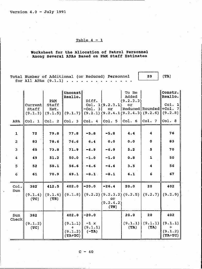
version 4.0 - July 1991
'rable 4 - 1
Worksheet for the Allocation of Patrol Personnel Among Several APAs Based on PAM Staff Estimates
Total Number of Additional (or Reduced) Personnel 20 (TA) for All APAs (9.1.1) •. . ••••.•...
Current Staff
(9.l.3)
PAM Staff Est.
(9.1.5)
unconst Reallo.
(9.1.7)
I i~d:~ I constr. Reallo.
Diff. (9.2.3.3) Col. 1(9.2.3.1) or I Col. 1
-Col. 31 or IReduced Rounded +Col. 7 (9.2.1) (9.2.4.1{9.2.4.3) (9.2.6) (9.2.8)
APA Col. 1 Col. 2 Col. 3 Col. 4 Col. 5 Col. 6 Col. 7 Col. 8
1 72 79.8 77.8 -5.8 -5.8 4.4 4 76
2 83 78.6 76.6 6.4 0.0 0.0 0 83
3 65 73.8 71.9 -6.9 -6.9 502 5 70
4 49 51.2 50.0 -1.0 -1.0 0.8 1 50
5 52 58.1 56.6 -4.6 -4.6 3.5 4 56
6 61 70.9 69.1 -8.1 -8.1 6.1 6 67
Col. 382 41205 402.0 -20.0 -26.4 20.0 20 402 Sum
Sum Check
(9.1.4) (9.1.6) (9.1.8) (9.2.2) (9.2.3.2) (9.2.5) 1 or 1 (9.2.4.2)
(9.2.7) (9.2.9) (TC) (TE)
382
(9.1.2) (TC)
402.0 -20.0
(9.1.1) +
(9.1.2) (TA+TC)
-1 x (9.1.1)
(-TA)
C - 40
(TN)
20.0 20
(9.1.1) (9.1.1) (TA) (TA)
402
(9.1.1) +
(9.1.2) (TA+TC)

Version 4.0 - July 1991
APPENDIX D: Derivations of the Major Formulas Used in PAM
The following ten sections contain derivations of all of the major formulas used in the PAM model and is intended for those users who wish to examine more closely the relationships between *the input data and the calculated results. For some derivations, familiarity with algebraic operations is needed to follow the discussion and considerable use is made of notational shortcuts to reduce the length of each ~ection. Since many of the notations are not used elsewhere in the Manual, definitions are supplied in each section as new terminology and variables are introduced.
D - 1

version 4.0 - July 1991
APPENDIX 0.1: Average Number of On-Duty Troopers (Nr ) Required Per Day Within the APA To Meet the Average Daily (Obligated Time) Workload, (3.3.3)
The formula in Worksheet 3 that is used to determine the average number of on-duty troopers required per day within the APA to meet the average daily obligated time workload is given by:
Nr (3.3.3) =
Total Average Daily obligated Time Workload (3.3.1)
Shift Length (3.3.2) (0.1.1)
where obligated time refers to the time required by all patrol units to respond to and service all C!<'S and accidents in the APA. (See page 3-17 in the ~anual for a more detailed discussion of obligated time.) The formula for Nr in Worksheet 3 is based on the assumption that all patrol units are one-trooper units only. An adjustment for two-trooper units is available in Worksheet 6.
The derivation of formula (0.1.1) is based on the recognition that, at a minimum, there mu~t be sufficient reactive patrol resources to provide enough on-uuty time (i.e., there must be enough patrol units) to respond to and service all reactive (obligated time) workload; that is,
Total Reactive Patrol
Resources =
Total Reactive Workload.
(0.1.2)
The total reactive workload for any period of time (days) can be measured by determining the total obligated time (TOT) required for all CFS and accidents during the period. The total reactive patrol resources for any period of time can be expressed in hours as:
Total Reactive Patrol
Resources = (0.1.3)
0-2

where~
version 4.0 - July 1991
the average number of on-duty troopers per day,
shift length in hours, and
total number of days in the time period used to measure the total obligated time workload.
Replacing total reactive patrol resources in (0.1.2) with (0.1.3) and replacing the total reactive workload with total obligated time (TOT) yields.
= TOT (0.1.4)
Solving (0.1.4) for Nr gives:
* TOT
= (D.1.5)
The expression TOT/D equals the average daily obligated time workload (ADOT); that is,
TOT ADOT = (D.1.6)
D
Replacing TOT/D with ADOT in (0.1.5) yields the result (D.1.1): that is,
ADOT (3. 3 . 1) Nr (3.3.3) = (D.l. 7)
Sl (3.3.2)
D - 3
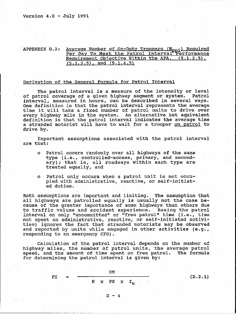
version 4.0 - July'1991
APPENDIX 0.2: Average Number of on-Duty Troopers (Nppi} Required Per Day To Meet the Patrol Inte~val ~erformance Requirement Objective within the APA r (5.1.2.5) r (5.1.3.5) rand (5.1.4.5)
Derivation of the General Formula for Patrol Interval
The patrol interval is a measure of the intensity or level of patrol coverage of a given highway segment or system. Patrol interval, measured in hours, can be described in several ways. One definition is that the patrol interval represents the average time it will take a fixed number of patrol units to drive over every highway mile in the system. An alternative but equivalent definition is that the patrol interval indicates the average time a stranded motorist will have to wait for a trooper on patrol to drive by.
Important assumptions associated with the patrol interval are that:
o Patrol occurs randomly over all highways of the same type (i.e., controlled-access, primary, and secondary); that is, all roadways within each type are treated equally, and
o Patrol only occurs when a patrol unit is not occupied with administrative, reactive, or self-initiated duties.
Both assumptions are important and limiting. The assumption that all highways are patrolled equally is usually not the case because of the greater importance of some highways than others due to traffic volume and accident experience. Basing the patrol interval on only "uncommitted" or "free patrol" time (Le., time not spent on administrative, reactive, or self-initiated activities) ignores the fact that stranded motorists may be observed and reported by units while engaged in other activities (e.g., responding to an emergency CFS).
Calculation of the patrol interval depends on the number of highway miles, the number of patrol units, the average patrol speed, and the amount of time spent on free patrol. The formula for determining the patrol interval is given by:
HM PI = (0.2.1)
N X PS x fu
D - 4

version 4.0 - July- 1991
where:
PI patrol interval (hours)q
HM total number of highway miles,
N total number of patrol units on duty,
PS average patrol speed (MPH), and
fu fraction of time spent on uncommitted time.
The derivation of formula (0.2.1) is mostly easily shown by starting with the definition that the patrol interval represents the average amount of time that it will take a fixed number of patrol units to cover the entire highway system. This definition can also be stated as a question: If it is known how many miles per hour all units drive collectively while on patrol, how many hours will it take to cover the entire highway system? The question implies that the total highway miles (HM) and the average miles driven per hour (ARM) by all units are known and are related to the patrol interval (PI) as:
HM = AHM x PI (0.2.2)
Rearranging the terms in (0.2.2) yields:
HM PI = (D.2.3)
AHM
The average number of highway miles driven per hour (ARM) by all units can be expressed as:
AHM = AM x N (0.2.4)
where:
N total number of units on duty, and
0-5
'------------------------------------ ~-------~ ----

Version 4.0 - July 1991
AM - average miles driven per hour per unit.
Replacing ARM in (0.2.3) with (0.2.4) yields:
HM PI = (0.2.5)
AM x N'
The average miles driven per hour by each unit (AM) can be expressed as:
AM = PS x fu (0.2.6)
where AM, PS, and fu are defined above. Replacing AM in (0.2.5) with (0.2.6) yields formula (0.2.1). For computational purposes, however, it is advantageous to express the fraction of time spent on uncommitted time as:
= (0.2.7) 60
where mu represents the average number of minutes per hour spent on uncommitr.ed time by each unit. Oividing mu by 60 yields the fraction of time spent on uncommitted time. Replacing fu in (D.2.6) with (0.2.7) yields:
AM = PS x (D.2.8) 60
and replacing AM in (D.2.5) with (D.2.8) yields the final expression for PI:
D - 6
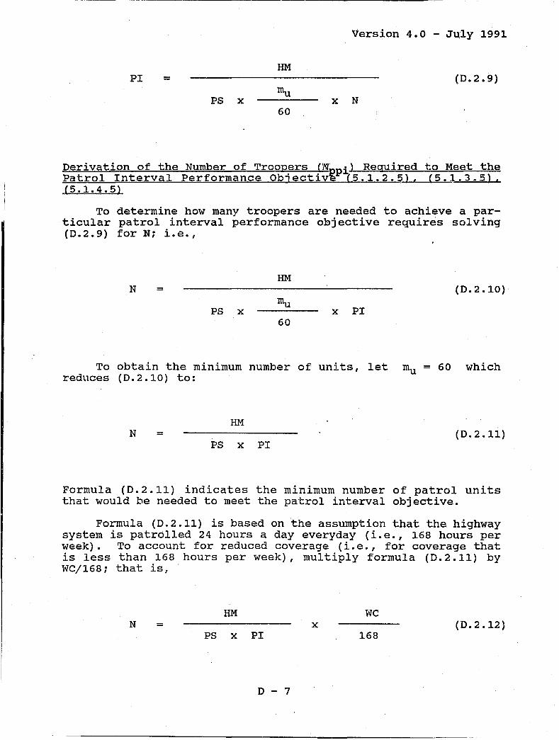
Version 4.0 - Ju,ly1991
HM PI = (0.2.9)
PS x x N 60
Derivation of the Number of Troopers (l~ppi) Required to Meet the Patrol Interval Performance Objectiv~ [5.1.2.5), (5.1.3.5) , (5.1.4.5)
To determine how many troopers are needed to achieve a particular patrol interval performance objective requires solving (0.2.9) for N; Le.,
HM N = (0.2.10)
PS x x PI 60
To obtain the m1n1mum number of units, let mu = 60 which reduces (0.2.10) to:
HM N = (0.2.11)
PS x PI
Formula (0.2.11) indicates the minimum number of patrol units that would be needed to meet the patrol interval objective.
Formula (0.2.11) is based on the assumption that the highway system is patrolled 24 hours a day everyday (i.e., 168 hours per week). To account for reduced coverage (i.e., for coverage that is less than 168 hours per week), multiply formula (0.2.11) by We/168; that is,
HM we N = x (D.2.12)
PS x PI 168
0-7

version 4.0 - July 1991
w~ere we represents the r.otal hours of coverage per week.
To determine the number of on-duty troopers that will be required per day (Nppi), use the relationship:
24 = N x (D.2.13)
where:
N number of patrol units given in (D.2.12), and
81 shift length in hours.
substituting (D.2.12) for N in (D.2.13) and simplifying yields:
HM x we = (D.2.14)
7 x PS x Sl x PI
which is the formula used in section 5.1 to determine the number of troopers required to meet patrol interval performance objectives for controlled-access highways (5.1.2.5), primary highways (5.1.3.5), and secondary highways (5.1.4.5). The sum of these results is recorded in (5.1.5)
D - 8

APPENDIX 0.3:
Version 4.0 - July 1991
Total Number of Troopers (~pir) Required Per Day within the APA To Provide Immediate Response To the Performance Objective Percentage of CFS, Accidents, and Self-Initiated Activities, (5.2.8)
In the PAM model, the appearance and serv1c1ng of CFS (i.e., accidents and other dispatched incidents) and self-initiated activities (e.g., motorist assists) are treated as a simple multiserver queuing process. CFS and self-initiated activities are assumed to occur randomly (i.e., as a Poisson process) and the service times associated with each activity are assumed to be independent and exponentially distributed.
The term "exponentially-distributed service times" describes the particular matherodi:ical distribution or formula that is used to describe the nature of the service times fqr dispatched CFS (e.g., what would the histogram of a sample of service times look like). A key property of exponentially-distributed service times is that the likelihood (or probability) of service time tl will be less than the likelihood (or probability) of service t1me t2 if t~ > t 2 • This property implies that the indiv"dual bars in the histogram of sample service times will be smal: .. er for longer service times. Field experience indicates that exponentiallydistributed service times are appropriate for describing many operations; for example, the lengths of telephone calls, the times required to complete transactions with bank tellers, the times required to checkout at grocery stores, and the average service times associated with dispatched CFS.
In a standard, steady-state queuing formulation with these assumptions and a fixed number of servers (i.e., a fixed number of patrol troopers), the average number of busy troopers at any given time (Nb ) is given by:
= CR x ST (0.3.1)
where CR represents the number of activities per hour and ST represents the average service time in hours.
The likelihood or probability that all of the troopers will be busy (Psat ) when the next activity occurs is called the "probability of saturation" and is given by Erlang's formula found in many introductory texts on queuing theory:
0-9

Version 4.0 - July 1991
= (D.3.2)
where NH represents the total number of troopers in the area, the term Nb t is interperted as Nb raised to the Nt th power, and
= N k
b
k! + (D.3.3)
Note that unless Nt equals or exceeds Nb'
there will not be enough troopers to handle the workload and the system will be continuously "saturated;" that is, the queue (or stack) wi],l grow larger and larger. Readers who wish to examine the derivation of these formulas as referred to any standard text on queueing theory or operations research such as Introduction to operations Research by Hillier and Lieberman (Holden-Day, Inc., 1967).
The likelihood or probability that at least one trooper will be available (Pavail) when the next activity occurs is given by:
Pavail = 1 (D.3.4)
For this derivation, the total number of troopers (Nt) available for assigned and self-initiated activities consists of the total number of on-duty troopers for reactive activities (Nr ) determined in Worksheet 3, the total number of on-duty troopers for self-initiated activities (Ns )' and the total number of onduty troopers for patrol activities (Np ); i.e.,
= + (D.3.5)
Troopers working on administrative activities (Na ) are assumed not to be available for field assignments. The number of on-duty troopers required for self-initiated activities per day can be determined from the number of on-duty troopers required per day for reactive activities (Nr ), the number of on-duty
D - 10
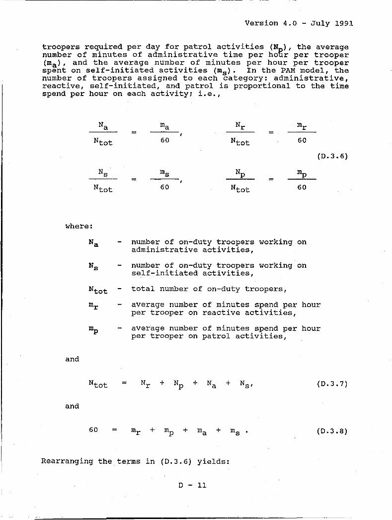
Version 4.0 - July 1991
troopers required per day for patrol activities (Np ), the average number of minutes of administrative time per hour per trooper (ma ) , and the average number of minutes per hour per trooper spent on self-initiated activities (ms )' In the PAM model, the number of troopers assigned to each category: administrative, reactive, self-initiated, and patrol is proportional to the time spend per hour on each activity; i.e.,
Na
Ntot
Ns
Ntot
where:
and
=
and
60 =
ma Nr mr = , =
60 Ntot 60
ms Np mp = =
60 Ntot 60
number of on-duty troopers working on administrative activities,
number of on-duty troopers working on self-initiated activities,
total number of on-duty troopers,
(0.3.6)
average number of minutes spend per hour per trooper on reactive activities,
average number of minutes spend per hour per trooper on patrol activities,
(D.3.7)
(0.3.8)
Rearranging the terms in (0.3.6) yields:
o - 11

~ __ "",.,_",,,,,,_,,,_,-,,,,,_,,,_,. __ .,.r~ .. _~" ________ ~ .. ·.-t""""'~'--I
version 4.0 - July 1991
= = =
Noting that the following is true:
= 60
and combining (0.3.9) and (D.3.10) yields:
=
Ntot
60 (0.3.9)
(0.3.10)
(D.3.11)
Using (0.3.8) to replace rnr + rnp with 60 - rna - rns in (D.3.11) yields:
= (D.3.12) 60
Using (D.3.12) to solve for Ns yields:
= (D.3.13)
where Ks equals:
= (D.3.14) 60
D - 12

version 4.0 - July 1991
Replacing Ns in (D.3.5) with (D.3.13) and rearranging yields:
= (D.3.15)
The right side of formula (D.3.15) consists of four terms. Three of the terms, Nr + (Ks x Nr ) + (Ks x Np )' represent the troopers that are busy on assigned and self-init~ated activities: i.e.,
= (D.3.16)
where Nr represents the troopers on reactive activities and (Ks x Nr ) + (Ks x N~) represents the troopers on self-initiated activit1es. The orriy troopers represented in formula in (D.3.15) that are not busy or available are represented by Np,. If no on-duty troopers are provided for patrol activities (i.e, if Np = 0), then Nt = Nr + (Ks x N ) which says that all troopers in the field are busy. The numEer of on-duty troopers required for reactive and self-initiated activities, Nr + (K x Nr ), is the minimum num~er of troopers required to handle t~e CFS and selfinitiated activities. Hence, by definition, if only Nr + (Ks x Nr ) troopers are available, every trooper will be busy for 60 m1nutes an hour which is equivalent to Psat = 1 and Pavail = o.
As troopers are added for patrol activities (i.e., as N becomes greater zero), Nt increases and the hourly reactiv~ and self-initiated workload for each trooper becomes less than 60 minutes per hour. As this happens, Psat decreases and P~va11 increases. As more troopers are added, Pavail increases unt1i 1t equals or exceeds the immediate response performance objective expressed as a probability (Pobj)i that is, Np is increased until
Pavail ~ Pobj (D.3.17)
where:
PIR% Pobj =
100
D - 13

Version 4.0 - July 1991
and PIR% represents the immediate response performance objective expressed as percent entered by the user in step 5.2.6.
Because of the complexity of formulas (D.3.2) and (D.3.3), it is not possible to derive a closed expression for Np based on Nr , Ks ' and Pob'. To overcome this difficulty, the PAM manual uses a table lo~-up procedure to determine N. Two options a.re available. The first option, described in se~ion 5.2 uses Table 3-1. This simplified procedure is based on three assumptions. The first is that Ks = 0.25. Use of this assumption permits the use of only one table and avoids the necessity for the user to calculate K. Using Ks = 0.25 is equivalent to using values of 9 and 15 minu~es per hour respectively for ma and ms. The second assumption is that staffing is uniform over all shifts. This assumption avoids the necessity of determining separate Np values for each shift. The third assumption is that the same performance objective (i.e., the same PIR% value) is used for each shift.
To use the procedure in section 5.2, the user must determine the average number of on-duty troopers per shift (Nrs ) in steps (5.2.1) through (5.2.5) and select an immediate response performance obj ecti ve percen.t (PIR%) in step (5. 2 . 6) . Once Nrs and; PIR% are known, Table 3-1 is used in step (5.2.7) to estimate the number of on-duty patrol troopers that are needed on each shift (Npir) to meet the immediate response objective. The total numbe~ of on-duty troopers for patrol per day, step (5.2.8), is obtained by mUltiplying the average number required per shift by the effective number of shifts per day.
If either or both of the simplifying assumptions used in section 5.2 are not valid, the user can use the Supplemental Worksheet in Appendix A in the Manual to estimate N ire This worksheet requires the use of rna and ms' determined inPworksheets 2 and 4, to calculate K (Step A.5.1). The value for Ks is used to select the appropria~e table based on the guidelines given on page A-6. The number of trooper8 required for patrol is determined for each shift (steps (A.6.1.3), (A.6.2.3), and (A.6.3.3», and the results are added together to obtain the total daily onduty requirement for patrol, Step (A.7).
The values in Table 3-1 and tables A-I through A-10 were determined using formulas (D.3.2), (D.3.3), (D.3.4), and (D.3.15) with the following logic:
o For a range of values (0.05 - 5.00) for the average number of on-duty troopers for reactive and selfinitiated activities on each shift (Nri) and a range of values (0.0 - 1.0) for Ks ' calculate p~v '1 values for integer values of Nt beginning with tfie smallest value of Nt such that Nt ~ Nr .
o For each value of Nt, determine the number of troopers available for patrol (Npir) based on (D.3.16): i. e. I
D - 14

o
Version 4.0 - July 1991
= (D.3.18)
Increase Nt until Pavail ~ .995.
Estimate Npir for specific values of Nr , Pavail' and Ks by int~rpolating between the calculated values for N ·r and Pavail for specific values for Ks. Each ~a\ue of K~ represents a separate table in Appendix F. with1n each table, each estimated value for Npir corresponds to specific values for Nr and Pavail·
D - 15

version 4.0 - July 1991
APPENDIX D.4: Average Number of On-Duty Troopers (Npapl Required within the APA To Meet the Average Trav~l Time Performance Objective for Area Patrol, (5.3.6.3)
In the PAM model, the average number of on-duty troopers required per day to meet the average travel time performance objective for area patrol is given by:
=
where:
A
A x we
7 x
average number of troopers required to meet the travel time performance objective for area patrol,
area (square miles) of the APA,
we coverage (hours) per week,
.NS number of shifts per day,
(D.4.1)
PTT average travel time (minutes) performance objective,
RS average response speed (MPH), and
81 shift length (hours).
Formula (D.4.1) is based on the so-called "square root law" which can be used to estimate the average travel distance (D) for a responding pol~ce unit in an area of size A with N available units. The generic formula is given by:
JA J N
(D.4.2) D = K x
where:
D - 16

version 4.0 - July 1991
D average distance (miles),
K a constant based on the geography of the area,
A the area of the region (square miles), and
N the number of police units available.
Using the time (T), speed (8), and distance (D) relationship from basic physics; i.e.,
o T = (0.4.3)
S
and replacing D in (0.4.3) with (0.4.2) yields:
K x j A T = (0.4.4)
s x j N
Under certain conditions, Larson (Urban Police Patrol Analysis, MIT Press, 1972) found that a value of 2/3 for the constant in (0.4.~) gives good results. (Key conditions are relatively low workload levels, uniformity of workload over the area, and ap-proximately equal travel times in all directions.) putting 2/3 in for K in formula (0.4.4) and multiplying by 60 to change travel time to minutes yields:
60 x 2 x j A T =
3 x S x j N (D.4.5)
Simplifying expression (0.4.5) yields:
40 x j A T =
s x j N (D.4.6)
D - 17

~~--~~--------~.-----------------------------------------------------------------------
version 4.0 - July 199J.
Solving formula (D.4.6) for N yields:
[ 40 r N = x A (D.4.7) T x S
Replacing speed (8) with the average response speed (RS) and time (T) with the average travel time performance objective (PTT) yields:
N = A (D.4.8)
which indicates the number of patrol units required each day to meet the performance travel time objective.
Formula (D.4.8) ~~ based on the assumption that the area is patroled 24 hours a day, 7 days a week (i.e., 168 hours per week). To account for reduced coverage (i.e., less than 168 hours per week), (D.4.8) can by multiplied by WC/168; that is,
WC N = A x (D.4.9)
168
where we represents the total hours of coverage per week.
Since each patrol unit represents one trooper, the total number of troopers needed per day for area patrol is given by:
24 = N x (D.4.10)
D - 18
I

version 4.0 - July 1991
where N is the number of units calculated in (0.4.9) and 8 1 is the shift length in hours. Replacing N in (0.4.10) with (0.4.9) and simplifying yields:
A x we = (0.4.11)
7 x
which is the formula given in (0.4.1). In section 5.3, formula (0.4.11) is used in step (5.3.6) to determine the number of troopers required to meet the target ~ravel time for area patrol.
D - 19

version 4.0 - July 1991
APPENDIX 0.5: Average Number of On-Duty Troopers (Np1p ) Required Within the APA To Meet the Average Trav~l Time Performance Objective for Line Patrol, (5.4.6)
In the PAM model, the average number of troopers required to meet the average travel time performance objective for line patrol is given by:
=
where:
L
NS
RS
PTT
we
20 x L x we (0.5.1)
7 x RS x PTT x
average number of troopers required to meet the travel time performance objective for line patrol,
highway miles in the line patrol segment,
number of shifts per day,
average response speed (MPH),
average travel time (minutes) performance objective,
coverage (hours) per week, and
shift length (hours).
The average travel distance to an incident on a highway segment patrolled by one unit is given by:
L o = (0.5.2)
3
where D represents the distance traveled in miles and L represents the number of miles in the highway segment. The basis for formula (0.5.2) is observation that if calls-for-service occur uniformly over the highway segment and the unit patrols uniformly
o - 20
I

version 4.0 - July 1991
over the segment, then the average distance between the unit and the location of the CFS is equivalent to the expected difference (or range) in a sample of two observations drawn from a uniform probability density function over the interval [O,L].
using the time (T), distance (D), and speed (S) relationship, D = S x T, and solving for T yields:
D T = (D.5.3)
S
Replacing D in (D.5.3) with formula (D.5.2) and multiplying by 60 to calculate travel time in minutes yields:
60 x L T = (D.5.4)
3 x S
Assuming that N units are used over the entire highway segment and each unit is assigned to a subsegment approximately equal to liN of the entire segment, then the average travel time formula for each sub segment becomes:
60 x (LIN) T = (D.5.5)
3 x S
Solving (D.5.5) for N and simplifying yields:
20 x L N = (D.5.5)
S x T
Replacing speed (S) with the average response speed (RS) and time (T) with the travel time performance objective for line patrol (PTT) in (D.5.6) yields:
D - 21

version 4.0 - July 1991
20 x L N = (0.5.6)
RS x PTT
Formula (0.5.6) indicates the m1n1ffium number of units (N) that are required each day to meet the travel time objective (PTT) for line patrol.
Formula (0.5.6) is based on the assumption that the highway segment is patroled 24 hours per day, 7 days a week (i.e, 168 hours per week). To account for reduced coverage (i.e., less than 168 hours per week), multiply (0.5.6) by We/168; that is,
20 x L we N = x (0.5.7)
RS x PTT 168
where we represents the total hours of coverage per week.
since each patrol unit has only one trooper, the number of on-duty troopers required per day (Np1p ) equals:
24 = N x (0.5.8)
where N is the number of units calculated in (0.5.7) and S1 is the shift length in hOurs. substituting (0.5.7) for N in (0.5.8) and simplifying yields:
20 x L x we = (0.5.9)
7 x RS x PTT x
Formula (0.5.9) is used in step (5.4.6) to determine Np1p .
o - 22

Version 4.0 - July 1991
APPENDIX D.6: Average Total Number of On-Duty Troopers (N) Required Per Day for All Patrol Activities within the APA, One Trooper Per unit, (6.1.5)
Introduction
The basic formula in the PAM model, used to derive the average daily number of on-duty troopers, is given by:
N =
1
where:
N
+ (D.6.1)
60 60
the average number of on-duty troopers per day (i.e., per 24-hour period),
the average number of on-duty troopers required per day for reactive activities,
the average number of on-duty troopers required per day for patrol activities,
average number of minutes spend per hour per trooper on administrative activities, and
average number of minutes spend per hour per trooper on self-initiated activities.
Four Workload Components
Derivation of formula (D.6.1) is based on the assumption that the average total number of on-duty troopers required per day (N) consists of four components; that is,
N = + + + (D.6.2)
where Nt, Nr, and Np are defined above and
D - 23

Version 4.0 - July 1991
the average number of on-duty troopers required per day for self-initiated activities, and
the average number of on-duty troopers required per day for administrative activities.
Much of the PAM model is devoted to providing the user with procedures for determining each of the four components identified above. The derivation of formula (D.6.1) is based on the procedures that are used to determine the number of troopers for each component. The procedure for each component is presented below.
Reactive and patrol activities. In the PAM model, the number of on-duty troopers required per day for reactive activities (Nr ) depends on two measures: (1) the total obligated time per day and (2) the shift length of the agency. Neither measure is dependent upon the total number of troopers (N) that are present. The number of on-duty troopers required per day for patrol activities (N ) is based on the availability of troopers for reactive and sel~initiated activities and trooper visibility for deterrence. The PAM model offers several options f9r determining Np based on the number of highway miles, patrol speed, patrol interval performance objectives set by the agency, area of the jurisdiction, response speed, and the number of on-duty troopers for reactive activities. Regardless of which option is used, all are independent of the total number of on-duty troopers (N). Hence, for both reactive and patrol activities, all of the workload measures are independent of the number of troopers that are available and, as a result, values for Nr and N can be obtained using historical data regardless of the staffi~g levels of the agency in the past.
Self-initiated and administrative activities. In contrast to the procedures used to determine Nr and Np ' the workload measures for Ns and N used in the PAM model are not independent of the number of on-guty troopers (N) that are present. The reason for this is the fact that for virtually all law enforcement agencies the amount of work that is recorded for administrative and self-initiated activities is, in fact, directly related to how many troopers are on-duty. The validity of this assertion is based on the following observations:
o Associated with each trooper is a certain amount of time that does not fall into either the reactive or self- initiated or patrol categories. As a result, the total administrative time for an agency is not fixed, but rather increases or decreases as the number of troopers increases or decreases.
o The total time devoted to self-initiated activities is also directly related to the number of troopers in the field; that is, as the number of troopers increases, the amount of self-initiated work increases. This occurs because the fraction of self-
D - 24

Version 4.0 - July 1991
initiated wcrk that can be performed with existing patrol resources is usually minor when compared to the total self-initiated work that could be pursued. As a result, there is, potentially, enough self-initiated work to absorb even a doubling or tripling of existing patrol resources.
Determination of Ns and Na
The dependency of Ns and Na upon the average total number of on-duty troopers per day (N) can be expressed as:
=
and
=
where:
(D.6.3)
(D.6.4)
fraction of time spend on self-initiated activities, and
fraction of time spend on administrative activities.
Inserting expressions (D.6.3) and (D.6.4) into (D.6.2) above yields:
N = + + (fs x N) + (fax N)
Solving (D.6.5) for N yields:
N = 1
Nr +
f a
The fractions fs and fa can be expressed as:
D - 25
(D.6.5)
(D.6.6)

version 4.0 - July 1991
fs rns
(0.6.7) = 60
and
fa rna
(0.6.8) = 60
where ms and ma are defined above. Placing expressions (D.6.7) and (D.6.8) into formula (D.6.5) yields the basic PAM formula:
+ N = (0.6.9)
1 60 60
D - 26

Version 4.0 - July 1991
APPENDIX D.7: Average Total Number of On-Duty Troopers (Nol Required Per Day for All Patrol Activities wi thin the APA, Adj usted fo!<;-., One and Two Trooper Units, (6.2.41
Determination of the total number of on-duty troopers required per day (No) is based on:
o the average total number of patrol units needed per day (NU ) , and
o the percent of patrol units that are staffed with two troopers (P2T%).
The average total number of patrol units needed per day (Nu ) is equal to the average total number of on-duty troopers needed each day if every patrol unit is staffed with only one trooper. The number of on-duty troopers required per day is calculated in step (6.1.5) of the PAM manual. (The derivation for the formula used in step (6.1.5) is given in section D.6 above.)
The percent of patrol units that are staffed with two troopers (P2T%) is entered by the user in step (6.2.1). Based on P2T%, define
P2T% f = (D.7.1)
100
where f, calculated in step (6.2.2), represents the fraction of units staffed with two troopers. using Nu and f, let
= (D.7.2)
where N2u represents the number of patrol units per day that are staffed with two troopers. If N1U represents the number of patrol units per day that are staffed with one trooper, then
= (D.7.3)
D - 27

version 4.0 - July 1991
Solving (D.7.3) for N1u and replacing N2u with (D.7.2) yields
=
=
= (1 - f) x Nu (D.7.3)
The total number of on-duty officers is given by
= + (D.7.4)
Replacing Nl~ with (D.7.3) and N2U with (D.7.2) in (D.7.4) and rearranging Ylelds:
= 1 x (1 - f) x Nu + 2 x (f x Nu )
= (1 + f) x Nu . (D.7.5)
Formula (D.7.5) is used in Step (6.2.4).
D - 28
I

Version 4.0 - July 1991
Appendix 0.8: Average Total Number of On-Duty Troopers (Not) and On-Duty Field Supervisors (Nos) Required Per Day For Patrol Activities ~ithin the APA, Adjusted for the Presence of Field Supervisors and Special Assignment Personnel, (7.2.4) and (7.3.1)
Introduction
The adjusted number of on-duty troopers required per day (Not) is based on the formula (7.2.4):
= x
where:
and
s
f
~o + + +
s
s + f
the unadjusted number of on-duty troopers required per day determined in Step (6.3.2) ;
the average span of control for field supervisors (i.e., the average number of troopers supervised by each field supervisor specified by the user in Step (1.2.3) and transferred to Step (7.1.1);
the fraction of supervisor on-duty time spent on patrol activities (i.e., non-supervisory activities); calculated in Step (7.1.3) ;
the fraction of on-duty time troopers assigned to special units spend on non-patrol activities; calculated in steps (7.2.1.5), (7.2.2.5), and (7.2.3.5) for special assignments 1, 2, and 3 respectively; and
D - 29
(0.8.1)

Version 4.0 - July 1991
the number of troopers assigned to special assignments 1, 2, and 3; user-supplied values entered in steps (7.2.1.2), (7.2.2.2), and (7.2.3.2) respectively.
The number of on-duty field supervisors required (Nos) is given by:
= (D.8.2) s
which is determined in step (7.3.1) of the Manual.
Derivation of the Formula for the Adjusted Number of On-Duty Troopers CNotl
If the percent of field supervisor on-duty time (Fs~) spent on patrol activities is known, the fraction (f) can be determined as:
f = (0.8.3) 100
The percent Fs~ is specified by the user in PAM in (1.2.4) and transferred toO (7.1.2). The calculation for (D.8.3) is step (7.1.3) in the manual.
If the percents of on-duty time (S~1' S~2' and S~3) that troopers assigned to special assignments 1~ 2, and 3 respectively spend on patrol activities are known, the fractions (fS1 ' fS2' and fS3) can be determined as:
100 = (D.8.4)
100
D - 30

version 4.0 - July 1991
100 8%2 fS2 = , and (0.8.5)
100
100 8%3 fs3 = (0.8.6)
100
The percents 8%1' 8%2 1 and 8%3 are supplied by the user,jn steps (7.2.1.3), (7.2.2.3), and (7.2.3.3); and calculatl.::ms for (0.8.4), (0.8.5), and (0.8.6) are completed in steps (7.2.1.5), (7.2.2.5), and (7.2.3.5) respectively.
The derivation of formula (0.8.1) depends on the observation that regardless of the values for s, Fs %' Ns1 ' Ns2 ' N~al 8%1' 8g,.2 f and 8g,.3 provided by the user, the total number of "full-tl.me equivalent fl on-duty troopers required per day after adjusting for the presence of field supervisors and troopers assigned to special units must equal the number of unadjusted on-duty troopers required per day (No) determined in Worksheet 6; that is:
= +
where:
+ + +
(0.8.7)
represents the adjusted number of on-duty troopers not assigned to a special unit;
represents the full-time equivalent number of troopers for patrol that will be provided by the presence of the Nos field supervisors;
represent the fraction of on-duty time troopers assigned to special units 1, 2, and 3 respectively spend on patrol activities
represents the full-time equivalent number of troopers for patrol that will be provided by the presence of the NSl troopers assigned to special assignment li
D - 31

version 4.0 - July 1991
=
represents the full-time equivalent number of troopers for patrol that will be provided by the presence of the NS2 troopers assigned to special assignment 2; and
represents the full-time equivalent number of troopers for patrol that will be provided by the presence of the NS3 troopers assigned to special assignment 3.
Replacing Nos in (0.8.7) with formula (0.8.2) yields:
+ f x + + + s
(0.8.8)
The term Not can be expressed as:
= (0.8.9)
Solving (0.8.9) for Naft yields:
= (0.8.10)
Replacing Naft in (0.8.8) with (0.8.10) and solving for Not yields:
Not = Kf x [No + Ns1 x (1-gs1 ) + Ns2 x (1-gs2 ) + NS3 x (1-gs3 )
(0.8.11)
where:
s Kf =
s + f
o - 32

Version 4.0 - July 1991
Formula (D.8.11) can be further simplified by noting that
(D.8.12)
which yields:
(D.8.13)
Using the results of (D.8.13) in (D.8.11) yields formula (D.8.1):
= x +
where:
s
s + f
+ + Ns3 x fS3]
(D.8.14)
The calculation of formula (D.8.14) in Worksheet 7 is completed in sections 7.1 and 7.2. The adjustment factor (Kf ) is calculated for step (7.1.5), and the term Kf x No is calculated in step (7.1.6). The remaining factors in (D.8.13) are calculated in steps (7.2.1.6), (7.2.2. 6), and (7. 2 • 3 . 6). The entire sum is produced for step (7.2.4).
Notice that if no patrol work is done by field supervisors (i.e., if f = 0) and no special assignment personnel are used (i.e., if Nsl = Ns2 = Ns3 = 0), then Not = No)·
D - 33

Version 4.0 - July 1991
APPENDIX D.9: Determination of the Shift Relief Factor (SRF) for the Calculation of the Total Number of Troopers !Nt) and Field Supervisors eNs) Required within the APA, (8.2.4), (8.3.1), and (8.3.2)
Introduction
The shift relief factor for a law enforcement agency is used to determine the total number of persons that an agency must have available (i.e., both on- and off-duty) in order to support a specified average number of on-duty troopers each day. The shift relief factor is defined as "the average number of persons required to cover one shift position every day."
For agencies with 8-hour shifts, shift relief factors typically fall in the range of 1.60 to 1.90. A shift relief factor of 1.70 for an agency using 8-hour shifts would indicate that the total staff for regular duty should be approximately 1.7 times the average number of on-duty positions that the agency plans to use per day. As an example, in order to cover 10 positions a day, this agency would have to have a total of 10 x 1.7 = 17 troopers available. (With 8-hour shifts and one trooper per unit, three positions are needed every day to support one 24-hour coverage unit.)
Shift relief factors increase as the shift length increases. Agencies using 10-hour shift will have shift relief factors in the range: 2.00 to 2.40. Relief factors for agencies with 12-hour shifts are 2.40 to 2.90.
Derivation of the Shift Relief Factor for Regular Duty
The shift relief factor is determined by the shift length, the work schedule us~d by the agency, the average amount of benefit time off given to each trooper, and the amount of time troopers spend on temporary special assignments. Calculation of the relief factor for an individual agency is usually based on data collected for one year and used in the following formula:
SRF = 365 x
Average Number of On-Duty Hours Per Trooper Per Year
D - 34
(D.9.1)
I

version 4.0 - July 1991
where:
8RF shift relief factor (number of troopers), and
81 shift length (hours).
The expression 365 x sl in (0.9.1) indicates the number of hours required to cover one position every day for an entire year. This value is calculated in step (8.2.2). The denominator in (0.9.2) is the average number of on-duty hours provided by each trooper in one year. This value is supplied by the user in step (8.2.3). Calculation of the shift relief factor is completed in step (8.2.4). The total number of troopers and total number of field supervisors required is calculated in steps (8.3.1) and (8.3.2).
Determination of the Average Number of on-Duty Hours Per Year Per Officer
One difficulty with the use of formula (0.9.1) is that few agencies actually keep track of hours worked. Rather, most personnel time-recording systems are designed to keep track of the amount of time off for each trooper (e.g." for vacation, holiday, personal leave, etc.). Recognizing that fact, it is often easier to determine the shift relief factor for an agency if formula (0.9.1) is rewritten as:
365 SRF =
x
Average Number of Off-Duty Hours Per Year Per Trooper
(0.9.2)
In this form, the average number of on-duty hours per year per trooper is calculated as:
Average Number of Off-Duty Hours Per Year Per Trooper.
(0.9.3)
The first term in (0.9.3) indicates the total number of hours that one trooper would be on-duty if he/she works every day of
o - 35

version 4.0 - July 1991
the year. The second term represents the average number of offduty hours per year per trooper. subtracting one term from the other in (D.9.3) gives the average number of on-duty hours per year per trooper. The usefulness of formula (D.9.2) is that it requires information (i.e., average time off per trooper) that is maintained by most agencies.
The average number of off-duty hours per year per trooper can be grouped into three categories:
o Regularly-scheduled days off given each week or schedule cycle. These are the days off every trooper receives because of the shift length, average work week, and particular work schedule being used. As an example, schedules based on 8-hour shifts and a 40-hour work week provide each trooper with an average of two days off per week.
o Benefit days off including vacation leave, holiday leave, personal time, compensatory time. The different kinds of benefit time off given varies from agency to agency and from one part of the country to another.
o Non-patrol time off includes those time when a trooper may be "on-duty,1l but is not on regular duty. For example, a trooper sent to a one-week training course in another state is obviously not available for regular duty, but is very likely still considered "on duty" while he is at the school. Whether non-regular duty time off should be included in the determination of the relief factor is not rigidly defined. An analyst trying to justify as many troopers as possible will likely include as much non-regular duty time off as possible in order to derive a higher relief factor. Another analyst, seeking to hold down staffing estimates, may exclude some non-regular duty time off to derive a lower value for the relief factor.
D - 36
~------------------------------------------------------------------I

Version 4.0 - July 1991
APPENDIX D.10: Allocation of Patrol Personnel Among Several APAs, Worksheet 9
Introduction
Worksheet 9 provides two methods for allocating a given number of staff among several APAs. Both methods rely on staffing estimates for each APA provided by the PAM model in worksheets 1 - 8. The first method, identified as "unconstrained allocation," indicates the ideal staffing if no limitations are imposed on how many troopers can be added or subtracted from the current staffing level in any APA (i.e., if there are no limitations on transfers between APAs). The second method, identified as "constrained allocation," can be used to determine staffing allocation when a fixed number of additional troopers are to be added to a group of APAs and no transfers of existing personnel are allowed. In this case, the no transfer constraint has the effect of insuring that no individual APA will lose staffing because of the allocation. The constrained allocation procedure can also be used to determine which APAs will lose personnel when staff reductions are required. In this case, the no transfer rule insures that no individual APA will gain personnel as a result of the overall staff reductions. All of the calculations for Worksheet 9 are summarized in Table 4-1.
The derivations below make use of the following notation:
T
TA
TA· -l.
TC
TC· -l.
TE
TB· -l.
total number of staff in all of the APAs after the reallocation,
total number of new staff (or total staff to be deleted) ,
total number of staff added to APA i (or staff deleted from APA i),
current total number of staff among all of the APAs,
current number of staff in APA i,
total number of staff estimated by the PAM model for all of the APAs,
total number of staff estimated by the PAM model for APA i, and
D - 37

version 4.0 - July 1991
T· 1 total number of staff in APA i after the reallocation.
The total staff to be allocated is given by:
T = TC + TA (D.10.l)
unconstrained Allocation
The rationale for the unconstrained allocation is that the total staff (T) should be distributed among the APAs in the same proportion as the PAM estimates; i.e.,
T· 1
T =
TE· 1
TE all APAs (D.10.2)
Solving for Ti and replacing T with (D.10.l) yields the formula for the number of staff that should be assigned to each APA;
T· 1 =
constrained Allocation
TA + TC (D.10.3)
TE
The total staff to be allocated is given by (D.10.l) above. The difference (di) for each APA between the number of staff provided by the unconstrained allocation for the APA (i.e, Ti given in (D.10.3» and the number of staff estimated for the APA by the PAM model (TEi)is given by:
d· 1 = T· 1 TE· 1 (D.10.4)
Expression (D.10.4) indicates whether an APA is under or overstaffed; i.e.,
D - 38
I

Version 4.0 - July 1991
if di > 0, the APA is overstaffed,
if di < 0, the APA is understaffed.
The di values are used to identify which APAs should gain (if TA > 0) and which APAs should lose staff (if TA < 0).
staff
Additional staff (TA > 0). If staff is to be added to APAs, the no transfer rule can be satisfied by distributing new staff only among those APAs that are understaffed (i.e., with di < 0). Let U represent the collection of APAs that understaffed and determine the total deficit staffing (TN) these APAs by summing the dis in U; i.e.,
the the
APAs are for
TN = d l + d 2 + d 3 + . . . + d n
-- only use APAs for which di < 0 --
(D.IO.5)
Allocation of the TA staff among the APAs in U is given by (D.IO.6) below where TAi represent~ the number of staff added to
APA i:
TA· 1 = TA
TN
The final allocation among all of the APAs is given by:
T· 1
T~ ~. 1 if d· ~ 0 1
if d· < 0 1
staff reduction (TA < 0). Fo~ staff reductions, strained allocation procedure uses the di values to those APAs that are overstaffed and, as a result, are for staff reductions. Let 0 represent the collection that are overstaffed and determine the total surplus (TN) for these APAs by summing the dis in 0; i.e.,
D - 39
(D.IO.6)
(D.10.7)
the conidentify eligible of APAs staffing

----------_._--------------------------------
version 4.0 - July 1991
TN = d 1 + d 2 + d 3 + . . . + dn
-- only use APAs for which di > 0 --
(0.10.8)
Allocation of the TA staff among the APAs in 0 is given by (0.10.9) below where TAi represents the number of staff to be taken from APA i:
TA· l. TA
TN (0.10.9)
Each TA· value for staff reductions will be a negative number. The final allocation among all of the APAs is given by:
T· l. = { Te· l. if d· ~ 0 l.
if d· > 0 l.
(0.10.10)
*U.S.GOV!RNMENTPRlNTINCOFFlCE: 1992.312.66765630
o - 40
I

DOT HS 807 793 December 1991