POLARIMETRY IN ASTROPHYSICS AND COSMOLOGY Lingzhen ...
207
POLARIMETRY IN ASTROPHYSICS AND COSMOLOGY by Lingzhen Zeng A dissertation submitted to The Johns Hopkins University in conformity with the requirements for the degree of Doctor of Philosophy. Baltimore, Maryland June, 2012 c Lingzhen Zeng 2012 All rights reserved
Transcript of POLARIMETRY IN ASTROPHYSICS AND COSMOLOGY Lingzhen ...
POLARIMETRY IN ASTROPHYSICS AND
COSMOLOGY
by
Lingzhen Zeng
A dissertation submitted to The Johns Hopkins University in conformity with the
requirements for the degree of Doctor of Philosophy.
Baltimore, Maryland
June, 2012
c© Lingzhen Zeng 2012
All rights reserved
Abstract
Astrophysicists are mostly limited to passively observing electromagnetic radia-
tion from a distance, which generally shows some degree of polarization. Polariza-
tion often carries a wealth of information on the physical state and geometry of the
emitting object and intervening material. In the microwave part of the spectrum,
polarization provides information about galactic magnetic fields and the physics of
interstellar dust. The measurement of this polarized radiation is central to much
modern astrophysical research.
The first part of this thesis is about polarimetry in astrophysics. In Chapter 1,
I review the basics of polarization and summarize the most important mechanisms
that generate polarization in astrophysics. In Chapter 2, I describe the data analysis
of polarization observation on M17 (a young, massive star formation region in the
Galaxy) from Caltech Submillimeter Observatory (CSO) and show the physics that
we learn about M17 from the polarimetry.
Polarimetry also plays an important role in modern cosmology. Inflation theory
predicts two types of polarization in the Cosmic Microwave Background (CMB) radi-
ation, called E-modes and B-modes. Measurements to date of the E-mode signal are
consistent with the predictions of anisotropic Thompson scattering, while the B-mode
signal has yet to be detected. The B-mode power spectrum amplitude can be param-
eterized by the relative amplitude of the tensor to scalar modes r. For the simplest
inflation models, the expected deviation from scale invariance (ns = 0.963± 0.012) is
coupled to gravitational waves with r ≈ 0.1. These considerations establish a strong
motivation to search for this remnant from when the universe was about 10−32 seconds
ii

old.
The second part of this thesis is about the Cosmology Large Angular Scale Sur-
veyor (CLASS) experiment, that is designed to have an unprecedented ability to
detect the B-mode polarization to the level of r ≤ 0.01. Chapter 3 is an introduction
to cosmology, including the big bang theory, inflation, ΛCDM model and polariza-
tion of the CMB radiation. Chapter 4 is about CLASS, including science motivation,
instrument optimization and lab testing.
Advisor: Prof. Charles L. Bennett
Second reader: Prof. Tobias Marriage
iii
Acknowledgements
The work described in this thesis would not have been possible without the support
of many people. Foremost, I would like to express my sincere gratitude to my advisor
Prof. Chuck Bennett for the continuous support of my Ph.D study and research, for
his patience, motivation, enthusiasm, and immense knowledge. His guidance helped
me in all the time of research and writing of this thesis. I could not have imagined
having a better advisor and mentor for my Ph.D study.
Besides my advisor, I would like to thank Dave Chuss. In many research projects,
I have been aided for many years by him. Dave is patient and always ready to discuss
whatever problems are on my mind. I would like to thank Prof. Giles Novak, who
offered me much advice and insight on the millimeter/submillimeter polarimetry. I
will miss the time when we worked together on Mauna Kea summit.
I gratefully acknowledge Prof. Toby Marriage for his valuable advice in lab dis-
cussions, supervision on lab instrument development. I would also like to thank Toby
for his great help in my job application.
I would like to thank David Larson and Joseph Eimer. We worked together for
many years and have so many useful discussions and collaborations.
My sincere thanks also goes to Ed Wollack, John Vaillancourt, George Voellmer,
Gary Hinshaw, John Karakla, Karwan Rostem, Tom Essinger-Hileman and Paul Mirel
for offering me help and discussions on the various research projects.
I thank my fellow graduate/undergraduate students in the research group at Johns
Hopkins University: Dominik Gothe, Zhilei Xu, Aamir Ali, Dave Holtz, Connor Hen-
ley and Tiffany Wei for the fun and proud of working together on the CLASS project.
It is a pleasure to thank my friends at JHU for making my life fun: Jiming Shi,
iv

Jianjun Jia, Jun Wu, Zhouhan Liang, Jian Su, Sunxiang Huang, Yuan Yuan, Longzhi
Lin, Hao Chang, Di Yang, Xin Guo, Jie Chen, Xiulin Sun, Jianhua Yu, Xin Yu, Wen
Wang, Hui Gao, Jinsheng Li, Jiarong Hong and Yuan Lu. I am grateful to many
others for making my time at JHU enjoyable. Unfortunately, there are too many to
name individually.
I would also like to thank my undergraduate classmates: Huaze Ding, Xiao Hu
and Jun Li for our longtime friendship. I wish all of you the best in the future.
Last but not the least, I would like to thank my family: my parents Xiangxiong
Zeng and Qiuying Li, for giving birth to me at the first place and supporting me
spiritually throughout my life, and my sister Lingfang Zeng and brother Lingyao
Zeng, for their understanding and support in so many years.
v
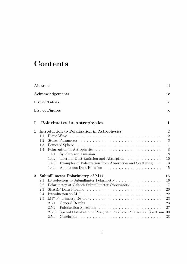
Contents
Abstract ii
Acknowledgements iv
List of Tables ix
List of Figures x
I Polarimetry in Astrophysics 1
1 Introduction to Polarization in Astrophysics 21.1 Plane Wave . . . . . . . . . . . . . . . . . . . . . . . . . . . . . . . . 21.2 Stokes Parameters . . . . . . . . . . . . . . . . . . . . . . . . . . . . 31.3 Poincare Sphere . . . . . . . . . . . . . . . . . . . . . . . . . . . . . . 71.4 Polarization in Astrophysics . . . . . . . . . . . . . . . . . . . . . . . 8
1.4.1 Synchrotron Emission . . . . . . . . . . . . . . . . . . . . . . 81.4.2 Thermal Dust Emission and Absorption . . . . . . . . . . . . 101.4.3 Examples of Polarization from Absorption and Scattering . . . 131.4.4 Anomalous Dust Emission . . . . . . . . . . . . . . . . . . . . 15
2 Submillimeter Polarimetry of M17 162.1 Introduction to Submillimter Polarimetry . . . . . . . . . . . . . . . . 162.2 Polarimetry at Caltech Submillimeter Observatory . . . . . . . . . . . 172.3 SHARP Data Pipeline . . . . . . . . . . . . . . . . . . . . . . . . . . 202.4 Introduction to M17 . . . . . . . . . . . . . . . . . . . . . . . . . . . 222.5 M17 Polarimetry Results . . . . . . . . . . . . . . . . . . . . . . . . . 23
2.5.1 General Results . . . . . . . . . . . . . . . . . . . . . . . . . . 232.5.2 Polarization Spectrum . . . . . . . . . . . . . . . . . . . . . . 272.5.3 Spatial Distribution of Magnetic Field and Polarization Spectrum 302.5.4 Conclusion . . . . . . . . . . . . . . . . . . . . . . . . . . . . . 38
vi
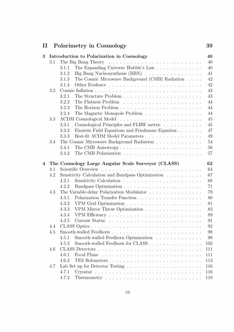
II Polarimetry in Cosmology 39
3 Introduction to Polarization in Cosmology 403.1 The Big Bang Theory . . . . . . . . . . . . . . . . . . . . . . . . . . 40
3.1.1 The Expanding Universe–Hubble’s Law . . . . . . . . . . . . . 403.1.2 Big Bang Nucleosynthesis (BBN) . . . . . . . . . . . . . . . . 413.1.3 The Cosmic Microwave Background (CMB) Radiation . . . . 423.1.4 Other Evidence . . . . . . . . . . . . . . . . . . . . . . . . . . 42
3.2 Cosmic Inflation . . . . . . . . . . . . . . . . . . . . . . . . . . . . . . 433.2.1 The Structure Problem . . . . . . . . . . . . . . . . . . . . . . 433.2.2 The Flatness Problem . . . . . . . . . . . . . . . . . . . . . . 443.2.3 The Horizon Problem . . . . . . . . . . . . . . . . . . . . . . . 443.2.4 The Magnetic Monopole Problem . . . . . . . . . . . . . . . . 44
3.3 ΛCDM Cosmological Model . . . . . . . . . . . . . . . . . . . . . . . 453.3.1 Cosmological Principles and FLRW metric . . . . . . . . . . . 453.3.2 Einstein Field Equations and Friedmann Equation . . . . . . . 473.3.3 Best-fit ΛCDM Model Parameters . . . . . . . . . . . . . . . . 49
3.4 The Cosmic Microwave Background Radiation . . . . . . . . . . . . . 543.4.1 The CMB Anisotropy . . . . . . . . . . . . . . . . . . . . . . . 563.4.2 The CMB Polarization . . . . . . . . . . . . . . . . . . . . . . 57
4 The Cosmology Large Angular Scale Surveyor (CLASS) 624.1 Scientific Overview . . . . . . . . . . . . . . . . . . . . . . . . . . . . 644.2 Sensitivity Calculation and Bandpass Optimization . . . . . . . . . . 67
4.2.1 Sensitivity Calculation . . . . . . . . . . . . . . . . . . . . . . 684.2.2 Bandpass Optimization . . . . . . . . . . . . . . . . . . . . . . 71
4.3 The Variable-delay Polarization Modulator . . . . . . . . . . . . . . . 794.3.1 Polarization Transfer Function . . . . . . . . . . . . . . . . . . 804.3.2 VPM Grid Optimization . . . . . . . . . . . . . . . . . . . . . 814.3.3 VPM Mirror Throw Optimization . . . . . . . . . . . . . . . . 834.3.4 VPM Efficiency . . . . . . . . . . . . . . . . . . . . . . . . . . 894.3.5 Current Status . . . . . . . . . . . . . . . . . . . . . . . . . . 91
4.4 CLASS Optics . . . . . . . . . . . . . . . . . . . . . . . . . . . . . . . 924.5 Smooth-walled Feedhorn . . . . . . . . . . . . . . . . . . . . . . . . . 98
4.5.1 Smooth-walled Feedhorn Optimization . . . . . . . . . . . . . 984.5.2 Smooth-walled Feedhorn for CLASS . . . . . . . . . . . . . . . 102
4.6 CLASS Detectors . . . . . . . . . . . . . . . . . . . . . . . . . . . . . 1114.6.1 Focal Plane . . . . . . . . . . . . . . . . . . . . . . . . . . . . 1114.6.2 TES Bolometers . . . . . . . . . . . . . . . . . . . . . . . . . . 113
4.7 Lab Set up for Detector Testing . . . . . . . . . . . . . . . . . . . . . 1164.7.1 Cryostat . . . . . . . . . . . . . . . . . . . . . . . . . . . . . . 1164.7.2 Thermometry . . . . . . . . . . . . . . . . . . . . . . . . . . . 118
vii
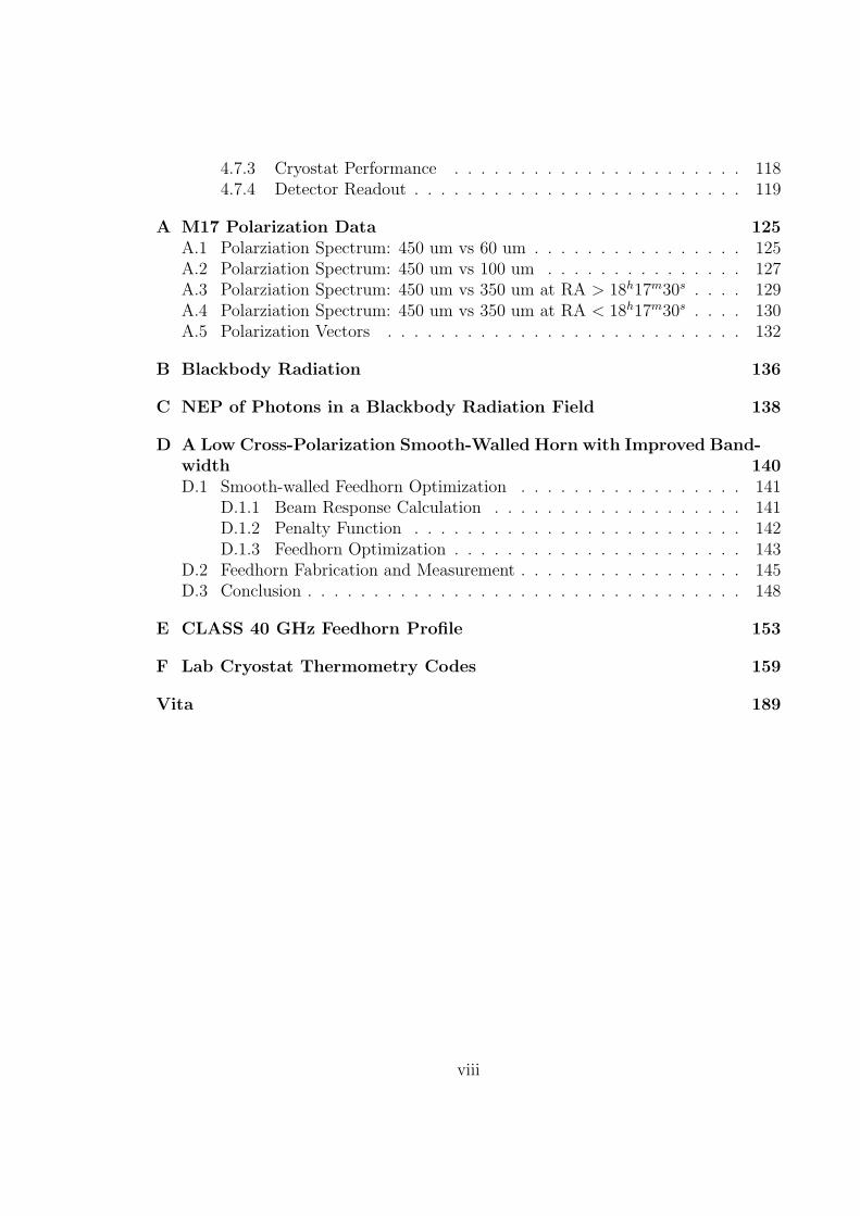
4.7.3 Cryostat Performance . . . . . . . . . . . . . . . . . . . . . . 1184.7.4 Detector Readout . . . . . . . . . . . . . . . . . . . . . . . . . 119
A M17 Polarization Data 125A.1 Polarziation Spectrum: 450 um vs 60 um . . . . . . . . . . . . . . . . 125A.2 Polarziation Spectrum: 450 um vs 100 um . . . . . . . . . . . . . . . 127A.3 Polarziation Spectrum: 450 um vs 350 um at RA > 18h17m30s . . . . 129A.4 Polarziation Spectrum: 450 um vs 350 um at RA < 18h17m30s . . . . 130A.5 Polarization Vectors . . . . . . . . . . . . . . . . . . . . . . . . . . . 132
B Blackbody Radiation 136
C NEP of Photons in a Blackbody Radiation Field 138
D A Low Cross-Polarization Smooth-Walled Horn with Improved Band-width 140D.1 Smooth-walled Feedhorn Optimization . . . . . . . . . . . . . . . . . 141
D.1.1 Beam Response Calculation . . . . . . . . . . . . . . . . . . . 141D.1.2 Penalty Function . . . . . . . . . . . . . . . . . . . . . . . . . 142D.1.3 Feedhorn Optimization . . . . . . . . . . . . . . . . . . . . . . 143
D.2 Feedhorn Fabrication and Measurement . . . . . . . . . . . . . . . . . 145D.3 Conclusion . . . . . . . . . . . . . . . . . . . . . . . . . . . . . . . . . 148
E CLASS 40 GHz Feedhorn Profile 153
F Lab Cryostat Thermometry Codes 159
Vita 189
viii
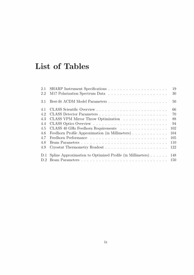
List of Tables
2.1 SHARP Instrument Specifications . . . . . . . . . . . . . . . . . . . . 192.2 M17 Polarization Spectrum Data . . . . . . . . . . . . . . . . . . . . 30
3.1 Best-fit ΛCDM Model Parameters . . . . . . . . . . . . . . . . . . . . 50
4.1 CLASS Scientific Overview . . . . . . . . . . . . . . . . . . . . . . . . 664.2 CLASS Detector Parameters . . . . . . . . . . . . . . . . . . . . . . . 704.3 CLASS VPM Mirror Throw Optimization . . . . . . . . . . . . . . . 884.4 CLASS Optics Overview . . . . . . . . . . . . . . . . . . . . . . . . . 944.5 CLASS 40 GHz Feedhorn Requirements . . . . . . . . . . . . . . . . 1024.6 Feedhorn Profile Approximation (in Millimeters) . . . . . . . . . . . . 1044.7 Feedhorn Performance . . . . . . . . . . . . . . . . . . . . . . . . . . 1054.8 Beam Parameters . . . . . . . . . . . . . . . . . . . . . . . . . . . . . 1104.9 Cryostat Thermometry Readout . . . . . . . . . . . . . . . . . . . . . 122
D.1 Spline Approximation to Optimized Profile (in Millimeters) . . . . . . 148D.2 Beam Parameters . . . . . . . . . . . . . . . . . . . . . . . . . . . . . 150
ix
List of Figures
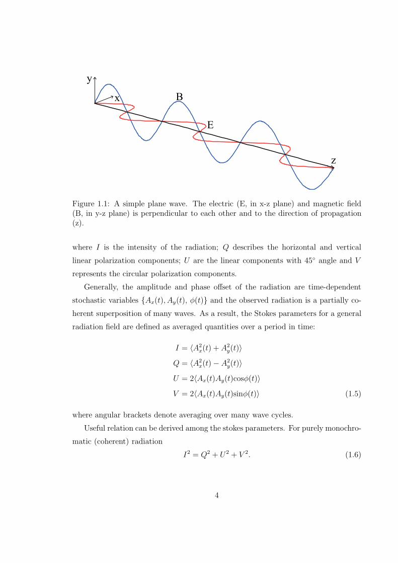
1.1 A simple plane wave. The electric (E, in x-z plane) and magnetic field(B, in y-z plane) is perpendicular to each other and to the direction ofpropagation (z). . . . . . . . . . . . . . . . . . . . . . . . . . . . . . . 4
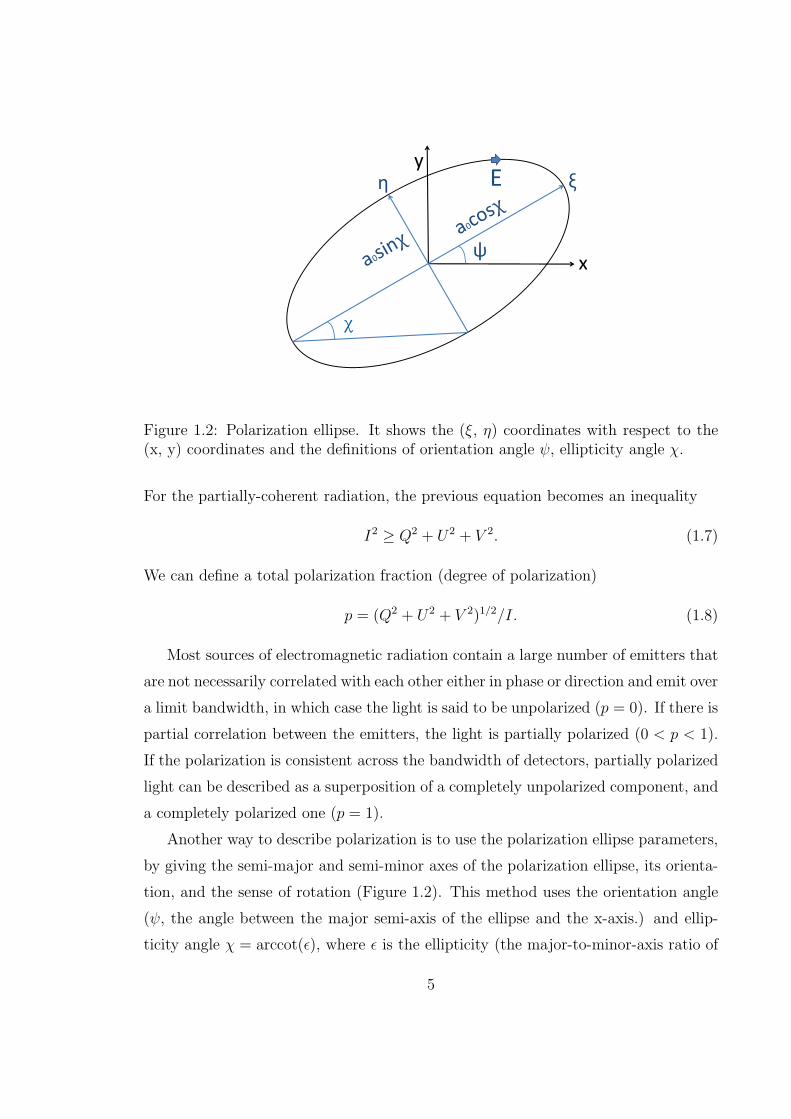
1.2 Polarization ellipse. It shows the (ξ, η) coordinates with respect to the(x, y) coordinates and the definitions of orientation angle ψ, ellipticityangle χ. . . . . . . . . . . . . . . . . . . . . . . . . . . . . . . . . . . 5
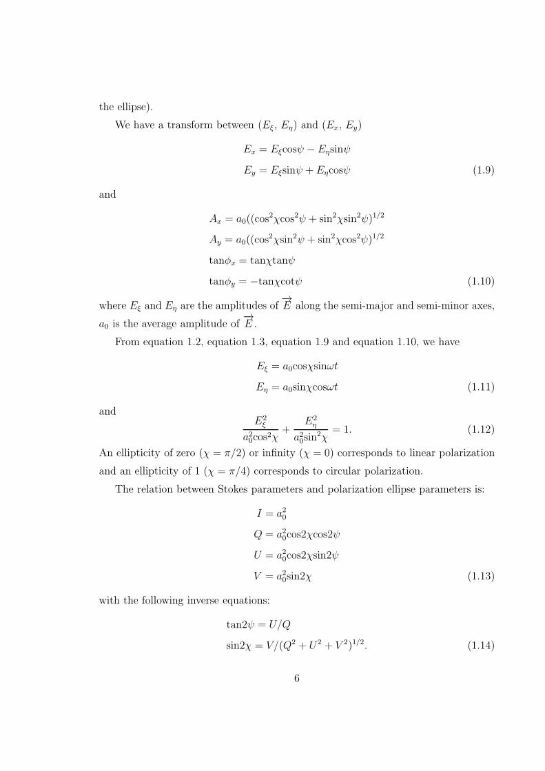
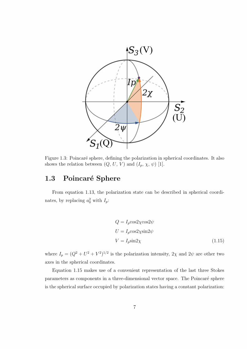
1.3 Poincare sphere, defining the polarization in spherical coordinates. Italso shows the relation between (Q, U , V ) and (Ip, χ, ψ) [1]. . . . . . 7
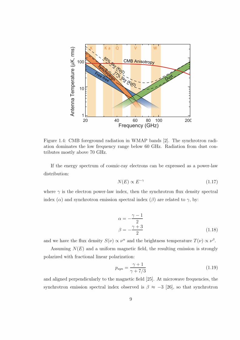
1.4 CMB foreground radiation in WMAP bands [2]. The synchrotron ra-diation dominates the low frequency range below 60 GHz. Radiationfrom dust contributes mostly above 70 GHz. . . . . . . . . . . . . . . 9
1.5 Starlight polarization vectors in Galactic coordinates. The upper panelshows polarization vectors in local clouds. The polarization averagedover many clouds in the Galactic plane is shown in the lower panel.The magnetic field is parallel to the polarization angle. . . . . . . . . 14
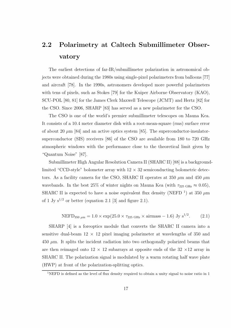
2.1 NEFD350 µm measurements (points) from Jan 2003 compared to theo-retical expectation (solid line) from equation 2.1 [3]. The performanceis about 1 Jy s1/2 for τ225 GHz = 0.05. . . . . . . . . . . . . . . . . . . 18
2.2 The polarization splitting optics of SHARP [4] for reconstituting theimage with an offset between the two polarization components. Left:The expanding beam from the CSO focus is reflected by P1 (paraboloid),F1 (flat mirror), through the HWP (half wave plate), and reaches theXG (crossed grid), where the polarization radiation is separated intotwo orthogonal (horizontal and vertical) components. Right: View to-ward the CSO focus. The vertical and horizontal components undergofurther reflections by a series of mirrors and grids, and are displacedlaterally at the BC (beam combiner), before being directed towardSHARC II. . . . . . . . . . . . . . . . . . . . . . . . . . . . . . . . . . 19
x
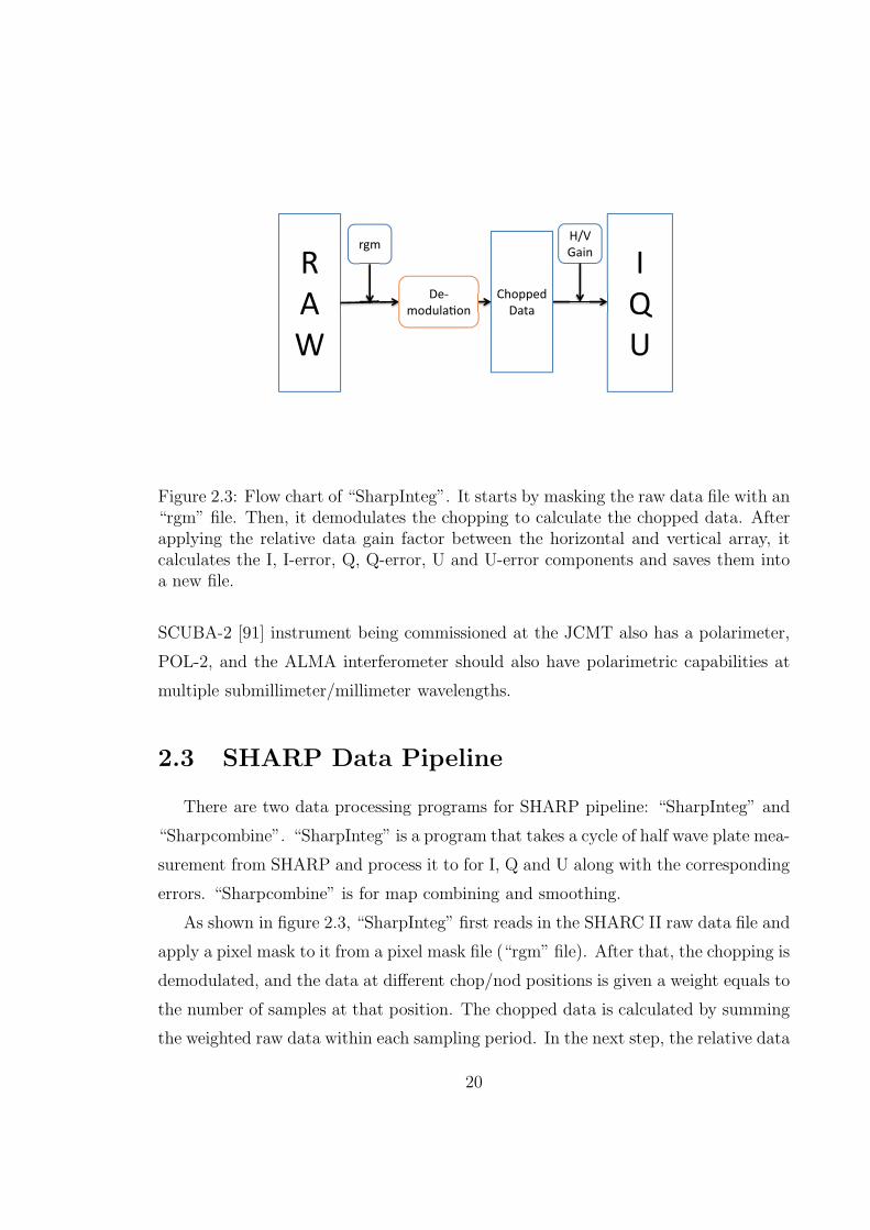
2.3 Flow chart of “SharpInteg”. It starts by masking the raw data filewith an “rgm” file. Then, it demodulates the chopping to calculate thechopped data. After applying the relative data gain factor between thehorizontal and vertical array, it calculates the I, I-error, Q, Q-error, Uand U-error components and saves them into a new file. . . . . . . . . 20
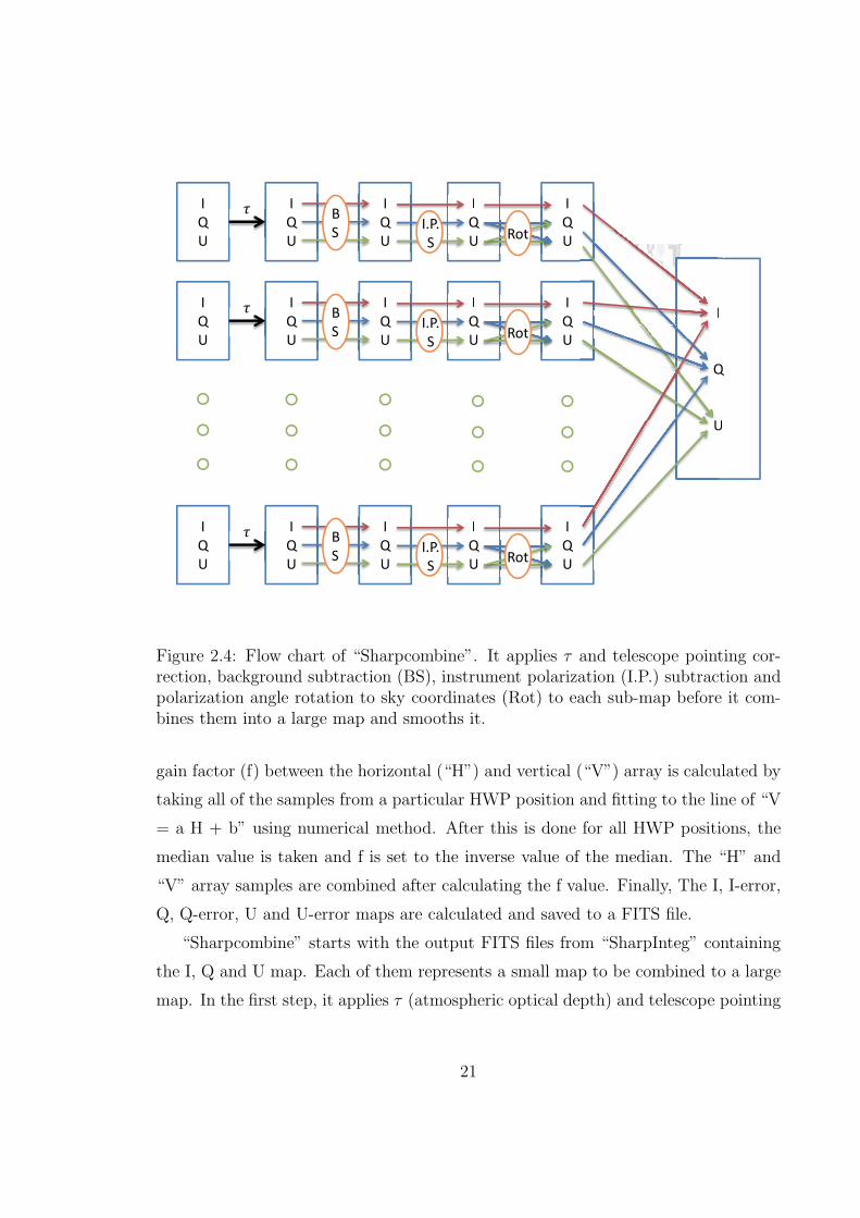
2.4 Flow chart of “Sharpcombine”. It applies τ and telescope pointingcorrection, background subtraction (BS), instrument polarization (I.P.)subtraction and polarization angle rotation to sky coordinates (Rot) toeach sub-map before it combines them into a large map and smooths it. 21
2.5 M17 is a premier example of a young, massive star formation regionin the Galaxy. Left: A M17 image from my 80 mm aperture opticaltelescope. Right: A false color image from Spitzer GLIMPSE (red: 5.8um; green: 4.5 um; blue: 3.6 um.) [5]. . . . . . . . . . . . . . . . . . . 22
2.6 A M17 model from [6]. The system can be described as a central clusterof stars surrounded by successive layers of H+, H0, and H2 gas, thatexpanding with different velocities to the outer side of the cloud. . . . 24
2.7 M17 polarization fraction vectors are plotted over the 450 um uncali-brated flux map. Thick vectors are detected with greater than or equalto 3σ level and thin vectors are between 2σ and 3σ level. The circle onthe bottom right shows the SHARP beamsize. Some parts of the fluxmap is removed due to high noise levels. Offsets are from 18h17m32s,-1614′25′′ (B1950.0). . . . . . . . . . . . . . . . . . . . . . . . . . . . 25
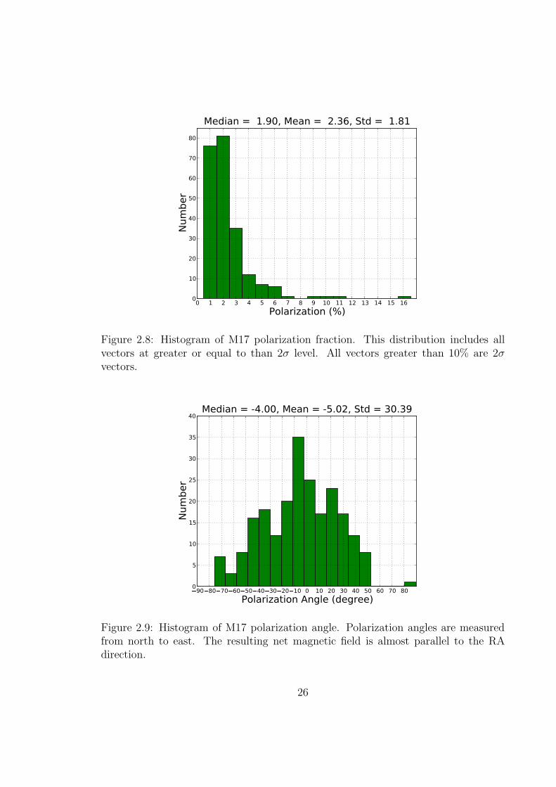
2.8 Histogram of M17 polarization fraction. This distribution includes allvectors at greater or equal to than 2σ level. All vectors greater than10% are 2σ vectors. . . . . . . . . . . . . . . . . . . . . . . . . . . . . 26
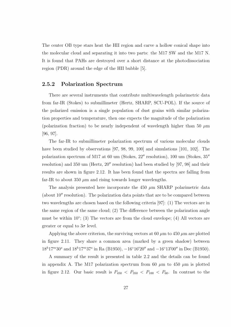
2.9 Histogram of M17 polarization angle. Polarization angles are measuredfrom north to east. The resulting net magnetic field is almost parallelto the RA direction. . . . . . . . . . . . . . . . . . . . . . . . . . . . 26
2.10 Magnetic field vectors from SHARP (red, 450 um), Stokes (green,100um) [7] and optical observation [8] (purple) plotted on top of SpitzerGLIMPSE 8.00 um flux map. The magnetic vectors from SHARPand Stokes are perpendicular to their polarization angles, while thosefrom optical polarization measurement are parallel to their polarizationangles. All magnetic vectors (plotted with the same length) are usedto indicate the direction only. Offsets are from 18h17m32s, -1614′25′′
(B1950.0). . . . . . . . . . . . . . . . . . . . . . . . . . . . . . . . . . 282.11 The common area (green shadow) for polarization spectrum analysis.
It is between 18h17m30s and 18h17m37s in Ra (B1950), −1616′20′′ and−1613′00′′ in Dec (B1950). The selected polarization vectors are at60 µm (yellow), 100 µm (green), 350 µm (blue) and 450 µm (red).Background is the 450 µm flux map. Offsets are from 18h17m32s, -1614′25′′ (B1950.0). . . . . . . . . . . . . . . . . . . . . . . . . . . . 29
xi
2.12 Polarization spectrum of some popular interstellar molecular clouds [9].The median polarization ratio are normalize by the value at 350 µm.In contrast to the results from other clouds, our work shows that, theM17 has lower median polarization at 450 µm than at 350 µm. Thepolarization spectrum falls monotonically from 60 µm to 450 µm. . . 31
2.13 Magnetic vectors from SHARP plotted over the [21 cm]/[450 µm] fluxratio map, showing that the shock front is passing through the cloud.The contour levels are 0.1, 0.3, 0.5, 0.7, 0.9. The “X” axis is definedby fitting contour level = 0.1. The new “X-Y” coordinate system isabout 66.3 with respect to the “Ra-Dec” coordinates. The shock isfollowing the “-Y” direction. The “y=0” and “y=-50 arcsec” lines sepa-rate the cloud into “post-shocked” (y > 0), “shock front” (-50 < y < 0)and “pre-shocked” (y < -50) regions. The polarization directions andmagnitudes in these regions are different (figure 2.14 and 2.15). Themagnetic fields in the dense cloud (can also be seen in figure 2.10) atthe top of the map survive the windswept. Offsets are from 18h17m32s,-1614′25′′ (B1950.0). . . . . . . . . . . . . . . . . . . . . . . . . . . . 33
2.14 Correlation between polarization angle and the Y direction (zero at18h17m32s, −1614′25′′), showing a linear relationship. The “post-shocked” region is at y > 0 and the “pre-shocked” region is at y < −50arcsec. . . . . . . . . . . . . . . . . . . . . . . . . . . . . . . . . . . . 34
2.15 Correlation between polarization fraction and Y direction (zero at18h17m32s, −1614′25′′), showing a “U” like shape. The polarizationfraction is higher at the “post-shocked” region at y > 0 and the “pre-shocked” region at y < −50 arcsec. . . . . . . . . . . . . . . . . . . . 34
2.16 Magnetic field vectors (red) and intensity contours of SHARP (green,levels = 0.0, 0.2, 0.4, 0.6, 0.8, 1.0) are over plotted on the 21 cmabsorption-line contour and the ratio of neutral HI (NHI) column den-sity to the spin temperature Tspin distribution map in the 17.5-22 km/svelocity area from [6]. This velocity component is correlated with the“post-shocked” and part of “shock front” region. The NHI/Tspin den-sity at the dense cloud region (see figure 2.13) is low. . . . . . . . . . 35
2.17 The [450 µm]/[350 µm] polarization ratio vectors over plotted on the[21 cm]/[450 µm] flux ratio map with contour levels = 0.1, 0.3, 0.5,0.7, 0.9. The blue (red) vectors represent P450 < (>) P350. Thelength of the 2% bar at bottom left is equivalent to P450/P350 = 1.0.The directions of the vectors are parallel to their polarization angles.Offsets are from 18h17m32s, -1614′25′′ (B1950.0). . . . . . . . . . . . 36
2.18 The [450 µm]/[350 µm] polarization ratio vectors and 450 µm intensitycontours of SHARP (green, levels = 0.0, 0.2, 0.4, 0.6, 0.8, 1.0) overplotted on the Fig.1 from [7]. The blue vectors is found to be correlatedwith the [OI] line, which is a tracer for the atomic gas. . . . . . . . . 37
xii
3.1 Timeline of the universe. The CMB radiation from the last scatteringsurface (LSS) when the universe is about 380,000 years old with thetemperature of about 3,000 K [10]. . . . . . . . . . . . . . . . . . . . 55
3.2 The internal linear combination map from WMAP [11], showing theall sky CMB temperature anisotropy. . . . . . . . . . . . . . . . . . . 56
3.3 The angular power spectrum from WMAP [12], showing the detectionof the first three peaks. The first peak is at ℓ ≈ 220, corresponding toan angular scale of about 1. . . . . . . . . . . . . . . . . . . . . . . . 58
3.4 Left: Quadrupole polarization from Thomson scattering of the CMBphotons with free electrons. Right: The E and B mode patterns. TheE-modes are curl-free components with no handedness. The B-modesare curl components with handedness. . . . . . . . . . . . . . . . . . . 59
3.5 Plots of signal for TT (black), TE (red ), and EE ( green). The not-yet-detected BB (blue dots) signal is from a model with r = 0.3. TheBB lensing signal is shown as a blue dashed line. The foreground modelfor synchrotron plus dust emission is shown as straight dashed lines [13]. 60
4.1 Two-dimensional joint marginalized constraint (68% and 95% CL) onscalar spectral index (ns) and tensor to scalar ratio (r), derived fromthe data combination of WMAP + BAO + H0 [14]. Three linear fitsare from different simple inflation models. . . . . . . . . . . . . . . . 63
4.2 The background is the WMAP 7 year all sky Q band polarization mapin Galactic coordinates showing the sky coverage of CLASS experi-ment. Observing from the Atacama Desert in Chile, CLASS covers∼ 65.1% of the sky above 45 elevation. Excluding the Galactic maskarea, the visible sky left is ∼ 46.8% (bright region). The dark circle atthe south pole is about 22 in radius. Figure courtesy of David Larson. 64
4.3 CLASS instrument overview for the 40 GHz band. The instrumentconsists a front-end variable-delay polarization modulator, catadioptricoptic system and a field cryostat. The lenses are cooled to about 4 Kand the smooth-walled feedhorn-coupled TES bolometer array operatesat 100 mK. Figure courtesy of Joseph Eimer. . . . . . . . . . . . . . . 65
4.4 CLASS wavebands and sensitivity curve from [15]. Left: The frequencybands of CLASS are chosen to straddle the Galactic foreground spec-tral minimum and to minimize atmospheric effects (see section 4.2.2).Right: The CLASS sensitivity curve, shown by the dashed curve alongthe shaded boundary, is the 1σ limit for each l and assumes 3 yearsof observing with a conservative 50% efficiency for down-time (see sec-tion 4.2.1). CLASS has the sensitivity to definitively detect B-modesat the cosmologically interesting limit of r ∼ 0.01. . . . . . . . . . . . 68
xiii
4.5 Annual variation of the Precipitable Water Vapor (PWV) content atChajnantor, based on 10 years of site testing. Conditions are worseduring the winter from the end of December to early April. The ex-pected median PWV for the rest of the year is around 1 mm, whileconditions of PWV < 0.5 mm can be expected up to 25% of the time[16]. . . . . . . . . . . . . . . . . . . . . . . . . . . . . . . . . . . . . 73
4.6 Atmospheric transmission and brightness temperature at CLASS sitefrom 5 to 1000 GHz. ATM parameters: ground temperature = 275 K,ground pressure = 558 mb, PWV = 1.0 mm, elevation = 45, altidude= 5180 m. ATM version: atm2011 03 15.exe. . . . . . . . . . . . . . . 74
4.7 Top: the CMB signal (equation 4.20) and Bottom: atmospheric noisesource (equation 4.16) for the relative signal-to-noise ratio calculation(equation 4.21). The red, green and blue lines shows our optimizedbandwidth for 40, 90 and 150 GHz band: (30.3 GHz - 40.3 GHz), (77.3GHz - 108.3 GHz) and (126.8 GHz - 164.3 GHz). . . . . . . . . . . . 77
4.8 The 2-D plot of relative signal-to-noise ratio (equation 4.22) from 0 to200 GHz showing our optimization results. The cross points of red,green and white lines are the locations of the local maxima. For the40 GHz band, we only search for the maximum in the range of ν > 30GHz. The coordinates are (30.3, 40.3), (77.3, 108.3) and (126.8, 164.3). 78
4.9 As shown in Poincare sphere, VPM modulates between Q and V , whilethe HWP mix Q and U . In the case of VPM, the residuals due to thespectral effects (shown in blue) are a function of measurable modula-tion parameters. Figure courtesy of David Chuss. . . . . . . . . . . . 79
4.10 VPM modulates polarization by introducing a controlled variable pathdifference between two orthogonal linear polarizations. Dots show thecomponent with polarization angle parallel to the grid; Double arrowshow that with angle perpendicular to the grid. By moving the mir-ror up and down, VPM introduces a path difference x(t) = 2d(t)cosθbetween these two orthogonal polarization components. . . . . . . . . 80
4.11 The wire grid performances for two different wavelengths from a sim-ulation [17]. In the limit of g/λ ≪ 1, a sinusoidal form for Stokes Qis in good agreement with an ideal grid (equation 4.29). The VPMreflection phase delay differs from the free-space grid-mirror delay ifthe conditions are changed. . . . . . . . . . . . . . . . . . . . . . . . 82
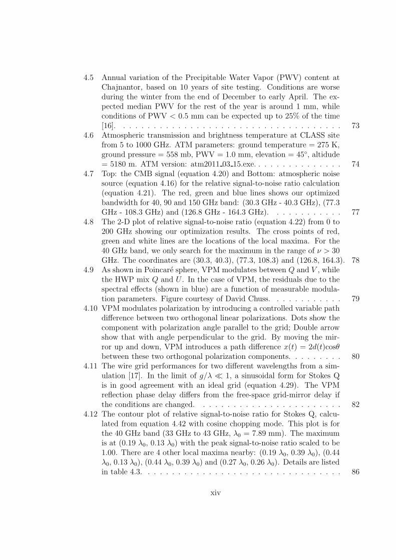
4.12 The contour plot of relative signal-to-noise ratio for Stokes Q, calcu-lated from equation 4.42 with cosine chopping mode. This plot is forthe 40 GHz band (33 GHz to 43 GHz, λ0 = 7.89 mm). The maximumis at (0.19 λ0, 0.13 λ0) with the peak signal-to-noise ratio scaled to be1.00. There are 4 other local maxima nearby: (0.19 λ0, 0.39 λ0), (0.44λ0, 0.13 λ0), (0.44 λ0, 0.39 λ0) and (0.27 λ0, 0.26 λ0). Details are listedin table 4.3. . . . . . . . . . . . . . . . . . . . . . . . . . . . . . . . . 86
xiv
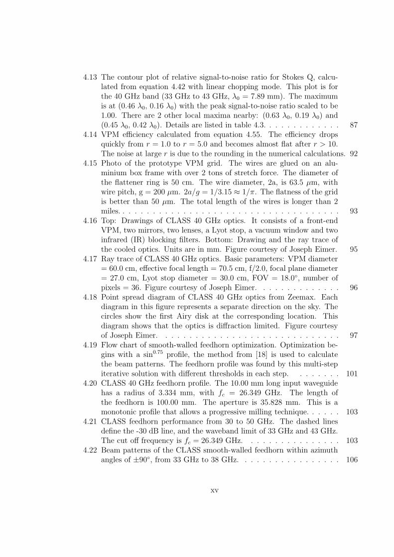
4.13 The contour plot of relative signal-to-noise ratio for Stokes Q, calcu-lated from equation 4.42 with linear chopping mode. This plot is forthe 40 GHz band (33 GHz to 43 GHz, λ0 = 7.89 mm). The maximumis at (0.46 λ0, 0.16 λ0) with the peak signal-to-noise ratio scaled to be1.00. There are 2 other local maxima nearby: (0.63 λ0, 0.19 λ0) and(0.45 λ0, 0.42 λ0). Details are listed in table 4.3. . . . . . . . . . . . . 87
4.14 VPM efficiency calculated from equation 4.55. The efficiency dropsquickly from r = 1.0 to r = 5.0 and becomes almost flat after r > 10.The noise at large r is due to the rounding in the numerical calculations. 92
4.15 Photo of the prototype VPM grid. The wires are glued on an alu-minium box frame with over 2 tons of stretch force. The diameter ofthe flattener ring is 50 cm. The wire diameter, 2a, is 63.5 µm, withwire pitch, g = 200 µm. 2a/g = 1/3.15 ≈ 1/π. The flatness of the gridis better than 50 µm. The total length of the wires is longer than 2miles. . . . . . . . . . . . . . . . . . . . . . . . . . . . . . . . . . . . . 93
4.16 Top: Drawings of CLASS 40 GHz optics. It consists of a front-endVPM, two mirrors, two lenses, a Lyot stop, a vacuum window and twoinfrared (IR) blocking filters. Bottom: Drawing and the ray trace ofthe cooled optics. Units are in mm. Figure courtesy of Joseph Eimer. 95
4.17 Ray trace of CLASS 40 GHz optics. Basic parameters: VPM diameter= 60.0 cm, effective focal length = 70.5 cm, f/2.0, focal plane diameter= 27.0 cm, Lyot stop diameter = 30.0 cm, FOV = 18.0, number ofpixels = 36. Figure courtesy of Joseph Eimer. . . . . . . . . . . . . . 96
4.18 Point spread diagram of CLASS 40 GHz optics from Zeemax. Eachdiagram in this figure represents a separate direction on the sky. Thecircles show the first Airy disk at the corresponding location. Thisdiagram shows that the optics is diffraction limited. Figure courtesyof Joseph Eimer. . . . . . . . . . . . . . . . . . . . . . . . . . . . . . 97
4.19 Flow chart of smooth-walled feedhorn optimization. Optimization be-gins with a sin0.75 profile, the method from [18] is used to calculatethe beam patterns. The feedhorn profile was found by this multi-stepiterative solution with different thresholds in each step. . . . . . . . 101
4.20 CLASS 40 GHz feedhorn profile. The 10.00 mm long input waveguidehas a radius of 3.334 mm, with fc = 26.349 GHz. The length ofthe feedhorn is 100.00 mm. The aperture is 35.828 mm. This is amonotonic profile that allows a progressive milling technique. . . . . . 103
4.21 CLASS feedhorn performance from 30 to 50 GHz. The dashed linesdefine the -30 dB line, and the waveband limit of 33 GHz and 43 GHz.The cut off frequency is fc = 26.349 GHz. . . . . . . . . . . . . . . . 103
4.22 Beam patterns of the CLASS smooth-walled feedhorn within azimuthangles of ±90, from 33 GHz to 38 GHz. . . . . . . . . . . . . . . . . 106
xv
4.23 Beam patterns of the CLASS smooth-walled feedhorn within azimuthangles of ±90, from 39 GHz to 44 GHz. . . . . . . . . . . . . . . . . 107
4.24 Beam patterns of the CLASS smooth-walled feedhorn within azimuthangles of ±15, from 33 GHz to 38 GHz. . . . . . . . . . . . . . . . . 108
4.25 Beam patterns of the CLASS smooth-walled feedhorn within azimuthangles of ±15, from 39 GHz to 44 GHz. . . . . . . . . . . . . . . . . 109
4.26 The averaged cross-pol, return-loss and edge-taper plot for the toler-ance calculation from 0 to 300 um. For each tolerance, these valueswere from the average of 120 calculations. (The plots are noisy at largetolerance, more calculation would be required to smooth the plots.) . 111
4.27 Section view of CLASS 40 GHz focal plane. It consists of a array of 36smooth-walled feedhorns, waveguide adapter, detector mounting plateand clips. The focal plane will operate at a temperature of 100 mK.Figure courtesy of Thomas Essinger-Hileman. . . . . . . . . . . . . . 112
4.28 The feedhorn-couple TES bolometers set up [15] and prototype de-tector chip for the 40 GHz CLASS [19]. Left: The detector set upshowing the feedhorn, detector housing, detector chip and backshort.Right: Photo of a 40 GHz prototype detector chip, showing the OMT,Magic Tees, filters and TES membranes. . . . . . . . . . . . . . . . . 113
4.29 The electro-thermal circuit diagram of a TES bolometer (modified from[20]). Left: Each pix with a heat capacity of C at temperature T isconnected by a thermal link G to a thermal source with a temperatureof Tbath. The total power to the pixel is Pγ + PJ − PG. Right: TESis biased by IB = VB/RB, in the case of RB ≫ RSH. For R ≫ RSH,the TES is bias by V = IBRSH, then fluctuations of R will result influctuation in current, which is read out by the inductor L and thesuperconducting quantum interference device (SQUID) amplifier. . . 114
4.30 Section view of model 104 Olympus ADR cryostat showing mechanicalheat switch controller, vacuum valve, pulse tube (PT) head, 60 K plate,4 K plate, adiabatic demagnetization refrigerator (ADR), high tempsuperconducting leads for 4 T magnet, thermal shielding, and vacuumjacket [21]. . . . . . . . . . . . . . . . . . . . . . . . . . . . . . . . . . 117
4.31 Left: The ADR and the He-4 refrigerator mounted on the 4 K plate ofthe HPD cryostat in the experimental cosmology lab at Johns HopkinsUniversity. Photo courtesy of David Larson. Right: the rack-mounteddevices for cryostat thermometry. From top to bottom, they are, aSRS SIM900 mainframe with 2 MUXs, a diode moniter and an ACbridge, a front panel, a NI GPIB to Ethernet adapter, a Lakeshore 370AC resistance bridge and two Keithley 2440 current sources. . . . . . 119
4.32 Cryostat cool down curves. It takes about 24 hours for the cryostat tocool down to the state with stable temperature readouts. The typicalvalues of the thermometers are listed in table 4.9. . . . . . . . . . . . 120
xvi
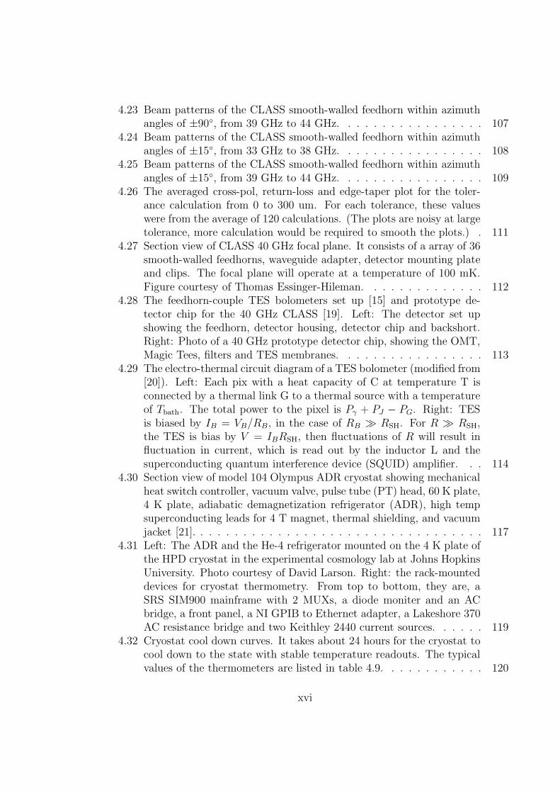
4.33 ADR cooling curves at 100 mK, showing the magnet current versustime of the ADR with the loads of from 2.0 to 10.0 µW. Based onthese curves, the FAA pill of the ADR have higher cooling capacitiesat lower loads. . . . . . . . . . . . . . . . . . . . . . . . . . . . . . . . 121
4.34 The FLL block diagram for TES detector readout, showing the coldelectronics inside the cryostat and the warm electronics (MCE) [22]. . 123
4.35 This photo shows the Multi-Channel Electronics (MCE) mounted onthe wall the cryostat in the experimental cosmology lab at Johns Hop-kins University. The MCE is connected to a data-acquisition computerby a pair of fiber optic cables (the orange wires). Photo courtesy ofDavid Larson. . . . . . . . . . . . . . . . . . . . . . . . . . . . . . . . 124
A.1 60 um polarization vectors from Stokes ([23], Yellow) and the 450um result from SHARP (smoothed to 22′′ resolution, Red), center at18h17m32s,-1614′25′′ (B1950.0). . . . . . . . . . . . . . . . . . . . . . 126
A.2 100 um polarization vectors from Stokes ([23], Green) and the 450umresult from SHARP (smoothed to 35′′ resolution, Red), center at 18h17m32s,-1614′25′′ (B1950.0). . . . . . . . . . . . . . . . . . . . . . . . . . . . 128
A.3 350 um polarization vectors from Hertz ([24]) and the 450 um resultfrom SHARP (smoothed to 20′′ resolution, Red), center at 18h17m32s,-1614′25′′ (B1950.0). Blue: Hertz vectors at RA > 18h17m30s, Green:Hertz vectors at RA < 18h17m30s . . . . . . . . . . . . . . . . . . . . 131
B.1 The Planck, Wien and Rayleigh-Jeans spectrum of a 2.725 K blackbody. The Wien limit is a good approximation at ν > 250 GHz andthe Rayleigh-Jeans limit works well below 20 GHz. . . . . . . . . . . 137
D.1 The initial, intermediate and final profiles are shown. All dimensionsare given in units of the cuttoff wavelength of the input circular waveg-uide. . . . . . . . . . . . . . . . . . . . . . . . . . . . . . . . . . . . . 145
D.2 (Top) The maximum cross-polar response across the band is shownfor the three profiles in Figure D.1. Measurements of the maximumcross-polarization are superposed. (Bottom) The reflected power mea-surements for the final feed horn are shown plotted over the predictedreflected power for the initial, intermediate, and final feedhorn profiles.Frequency is given in units of the cutoff frequency of the input circularwaveguide. . . . . . . . . . . . . . . . . . . . . . . . . . . . . . . . . . 146
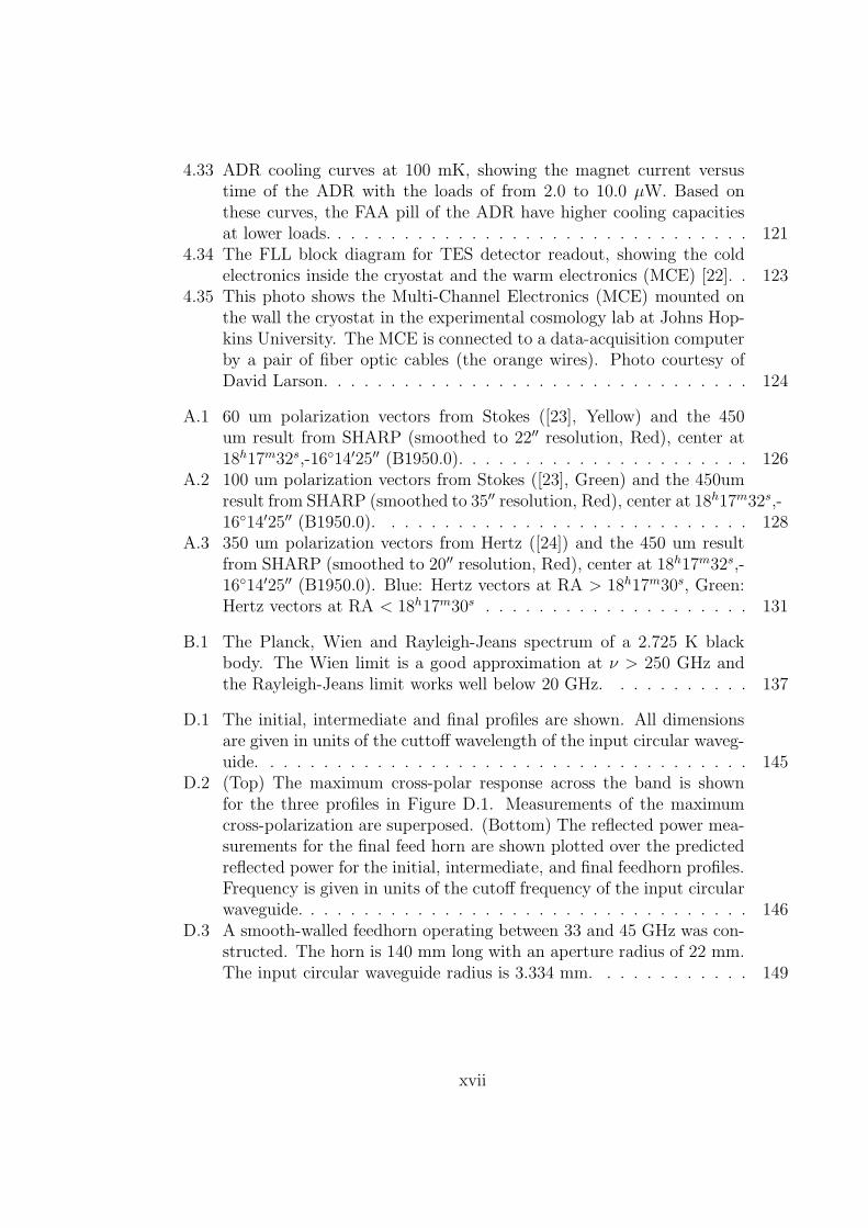
D.3 A smooth-walled feedhorn operating between 33 and 45 GHz was con-structed. The horn is 140 mm long with an aperture radius of 22 mm.The input circular waveguide radius is 3.334 mm. . . . . . . . . . . . 149
xvii
D.4 The measured E-, H-, and diagonal-plane angular responses for thelower edge (33 GHz), center (39 GHz), and upper edge (45 GHz) ofthe optimization band are shown. The cross-polar patterns in thediagonal plane are shown in the bottom three panels for each of thethree frequencies. . . . . . . . . . . . . . . . . . . . . . . . . . . . . 151
D.5 The maximum cross-polar response of the prototype feedhorn is com-pared to other implementations of smooth-walled feedhorns. The datapresented have been normalized to the design center frequencies asspecified by the respective authors. . . . . . . . . . . . . . . . . . . . 152
F.1 SRS readout program front panel. . . . . . . . . . . . . . . . . . . . . 160F.2 PID control program front panel. . . . . . . . . . . . . . . . . . . . . 160F.3 Block diagram of the SRS readout program. . . . . . . . . . . . . . . 161F.4 Block diagram of the PID control program. Part 1 of 3. . . . . . . . . 162F.5 Block diagram of the PID control program. Part 2 of 3. . . . . . . . . 163F.6 Block diagram of the PID control program. Part 3 of 3. . . . . . . . . 164
xviii
Part I
Polarimetry in Astrophysics
1
Chapter 1
Introduction to Polarization in
Astrophysics
Astrophysicists are mostly limited to passively observing electromagnetic radiation
from a distance. This radiation is most generally described by a specific intensity
as a function of sky direction (θ, φ), frequency (ν) and polarization state. The
polarization information is important for astronomy. Radiation from astronomical
sources generally shows some degree of polarization. Although it is usually only
a small fraction of the total radiation, the polarization component often carries a
wealth of information on the physical state and geometry of the emitting object and
intervening material. In the microwave part of the spectrum, polarization provides
information about galactic magnetic fields and the physics of interstellar dust. The
measurement of this polarized radiation is central to much modern astrophysical
research.
1.1 Plane Wave
Polarization describes the orientation and phase coherence of the oscillations of
electromagnetic waves. Specifically, the polarization of a wave is described by spec-
ifying the orientation of the wave’s electric field at a point in space. Polarization is
most usefully illustrated using the concept of a plane wave, a monochromatic wave
2
having planar wave fronts that are infinite in extent. Figure 1.1 shows a simple plane
wave with its electric component parallel to the x axis.
Generally, the electric field of a plane wave can be written as:
~E(~r, t) = (Ex, Ey, Ez) = (Axcos(kz − ωt+ φx), Aycos(kz − ωt+ φy), 0) (1.1)
where (Ax, Ay) and (φx, φy) are the amplitudes and phase offsets of the x and y
component of the electric field; ω is the angular frequency; k is the wave number.
In the x− y plane, equation 1.1 can be simplified as:
Ex = Axsin(ωt− φx)
Ey = Aysin(ωt− φy). (1.2)
By defining φ = φx − φy, equation 1.2 can be written into an elliptical form:
E2x
A2x
+E2
y
A2y
− 2ExEy
AxAycosφ = sin2φ. (1.3)
For different phase offsets, the polarization state varies. From equation 1.3, if
φ = mπ (where m = 0,±1,±2, ...), then Ex/Ax ± Ey/Ay = 0 (linear polarization); if
φ = (2m+1)π/2 and Ax = Ay, then E2x+E
2y = A2
x (circular polarization); if φ 6= mπ,
then it will be an elliptical polarization. In the latter cases (circular and elliptical
polarization), the oscillations can rotate either towards the right (0 < φ < π) or
towards the left (−π < φ < 0) in the direction of propagation.
1.2 Stokes Parameters
The parameters Ax, Ay, φ above, used to describe polarization have different
units. In 1852, George G. Stokes defined a set of 4 parameters (the Stokes parame-
ters) as a mathematically convenient alternative. For the monochromatic plane wave
described above, the Stokes parameters are:
I = A2x + A2
y
Q = A2x −A2
y
U = 2AxAycosφ
V = 2AxAysinφ (1.4)
3
y
x
z
E
B
Figure 1.1: A simple plane wave. The electric (E, in x-z plane) and magnetic field(B, in y-z plane) is perpendicular to each other and to the direction of propagation(z).
where I is the intensity of the radiation; Q describes the horizontal and vertical
linear polarization components; U are the linear components with 45 angle and V
represents the circular polarization components.
Generally, the amplitude and phase offset of the radiation are time-dependent
stochastic variables Ax(t), Ay(t), φ(t) and the observed radiation is a partially co-
herent superposition of many waves. As a result, the Stokes parameters for a general
radiation field are defined as averaged quantities over a period in time:
I = 〈A2x(t) + A2
y(t)〉
Q = 〈A2x(t)− A2
y(t)〉
U = 2〈Ax(t)Ay(t)cosφ(t)〉
V = 2〈Ax(t)Ay(t)sinφ(t)〉 (1.5)
where angular brackets denote averaging over many wave cycles.
Useful relation can be derived among the stokes parameters. For purely monochro-
matic (coherent) radiation
I2 = Q2 + U2 + V 2. (1.6)
4
ψ x
y ξ η
E
χ
Figure 1.2: Polarization ellipse. It shows the (ξ, η) coordinates with respect to the(x, y) coordinates and the definitions of orientation angle ψ, ellipticity angle χ.
For the partially-coherent radiation, the previous equation becomes an inequality
I2 ≥ Q2 + U2 + V 2. (1.7)
We can define a total polarization fraction (degree of polarization)
p = (Q2 + U2 + V 2)1/2/I. (1.8)
Most sources of electromagnetic radiation contain a large number of emitters that
are not necessarily correlated with each other either in phase or direction and emit over
a limit bandwidth, in which case the light is said to be unpolarized (p = 0). If there is
partial correlation between the emitters, the light is partially polarized (0 < p < 1).
If the polarization is consistent across the bandwidth of detectors, partially polarized
light can be described as a superposition of a completely unpolarized component, and
a completely polarized one (p = 1).
Another way to describe polarization is to use the polarization ellipse parameters,
by giving the semi-major and semi-minor axes of the polarization ellipse, its orienta-
tion, and the sense of rotation (Figure 1.2). This method uses the orientation angle
(ψ, the angle between the major semi-axis of the ellipse and the x-axis.) and ellip-
ticity angle χ = arccot(ǫ), where ǫ is the ellipticity (the major-to-minor-axis ratio of
5
the ellipse).
We have a transform between (Eξ, Eη) and (Ex, Ey)
Ex = Eξcosψ − Eηsinψ
Ey = Eξsinψ + Eηcosψ (1.9)
and
Ax = a0((cos2χcos2ψ + sin2χsin2ψ)1/2
Ay = a0((cos2χsin2ψ + sin2χcos2ψ)1/2
tanφx = tanχtanψ
tanφy = −tanχcotψ (1.10)
where Eξ and Eη are the amplitudes of−→E along the semi-major and semi-minor axes,
a0 is the average amplitude of−→E .
From equation 1.2, equation 1.3, equation 1.9 and equation 1.10, we have
Eξ = a0cosχsinωt
Eη = a0sinχcosωt (1.11)
andE2
ξ
a20cos2χ
+E2
η
a20sin2χ
= 1. (1.12)
An ellipticity of zero (χ = π/2) or infinity (χ = 0) corresponds to linear polarization
and an ellipticity of 1 (χ = π/4) corresponds to circular polarization.
The relation between Stokes parameters and polarization ellipse parameters is:
I = a20
Q = a20cos2χcos2ψ
U = a20cos2χsin2ψ
V = a20sin2χ (1.13)
with the following inverse equations:
tan2ψ = U/Q
sin2χ = V/(Q2 + U2 + V 2)1/2. (1.14)
6
(V)
(U)
(Q)
Figure 1.3: Poincare sphere, defining the polarization in spherical coordinates. It alsoshows the relation between (Q, U , V ) and (Ip, χ, ψ) [1].
1.3 Poincare Sphere
From equation 1.13, the polarization state can be described in spherical coordi-
nates, by replacing a20 with Ip:
Q = Ipcos2χcos2ψ
U = Ipcos2χsin2ψ
V = Ipsin2χ (1.15)
where Ip = (Q2 + U2 + V 2)1/2 is the polarization intensity, 2χ and 2ψ are other two
axes in the spherical coordinates.
Equation 1.15 makes use of a convenient representation of the last three Stokes
parameters as components in a three-dimensional vector space. The Poincare sphere
is the spherical surface occupied by polarization states having a constant polarization:
7
S =1
Ip
Q
U
V
(1.16)
The Poincare sphere provides a convenient way of representing polarization and
representing how any given retarder (i.e. the VPM described in section 4.3) will
change the polarization form. The north and south poles of the sphere represent
left and right circular polarization (V ). The points on the equator correspond to
linear polarization state (Q and U). Other points on the sphere represent elliptical
polarizations. If an arbitrarily chosen point on the equator designates horizontal
polarization, then the point which locates 180 opposite to it designates vertical
polarization. A general point (Ip) on the surface of the Poincare sphere is specific in
terms of the longitude (2ψ) and the latitude (2χ). The factor of 2 before ψ represents
the fact that any polarization ellipse is indistinguishable from one rotated by 180,
and the factor of 2 before χ indicates that an ellipse is indistinguishable from one
with the semi-axis lengths swapped by a 90 rotation.
1.4 Polarization in Astrophysics
Many mechanisms generate polarized emission in astrophysics, including syn-
chrotron emission, dust emission, absorption (extinction) and scattering, such as
starlight polarization and free-free (bremsstrahlung) emission from cloud edges. Ad-
ditional polarized components like the anomalous emission from dust have also been
discovered.
1.4.1 Synchrotron Emission
Synchrotron emission arises from the acceleration of cosmic-ray electrons in mag-
netic fields. Based on the results of Cosmic Microwave Background (CMB) foreground
studies [2] (Figure 1.4), synchrotron radiation dominates at frequencies below 60 GHz
(≥ 5 mm).
8
K K a Q V W
CMB Anisotropy
Frequency (GHz)
Ante
nna
Tem
pera
ture
(K,
rms)
1
10
100
10020 6040 80 200
85%Sky (Kp2)
Synchrotron
Free-free Dust
Synchrotron
77%Sky (Kp0)
Figure 1.4: CMB foreground radiation in WMAP bands [2]. The synchrotron radi-ation dominates the low frequency range below 60 GHz. Radiation from dust con-tributes mostly above 70 GHz.
If the energy spectrum of cosmic-ray electrons can be expressed as a power-law
distribution:
N(E) ∝ E−γ (1.17)
where γ is the electron power-law index, then the synchrotron flux density spectral
index (α) and synchrotron emission spectral index (β) are related to γ, by:
α = −γ − 1
2
β = −γ + 3
2(1.18)
and we have the flux density S(ν) ∝ να and the brightness temperature T (ν) ∝ νβ .
Assuming N(E) and a uniform magnetic field, the resulting emission is strongly
polarized with fractional linear polarization:
psyn =γ + 1
γ + 7/3(1.19)
and aligned perpendicularly to the magnetic field [25]. At microwave frequencies, the
synchrotron emission spectral index observed is β ≈ −3 [26], so that synchrotron
9
emission could have fractional polarization as high as psyn = 75% (equation 1.18
and equation 1.19), which is almost never observed. The main reason for that is the
magnetic field distribution and the electron energy distribution are not uniform in the
Galaxy. The line of sight and beam averaging effects reduce the observed polarization
fraction by averaging over different regions in the Galaxy. At low frequencies (below
a few GHz) Faraday rotation (∝ λ2) will also reduce the polarization fraction for a
sufficiently wide passband.
1.4.2 Thermal Dust Emission and Absorption
The dominant source of Galactic emission at far-infrared (far-IR) and submillime-
ter (SMM) wavelengths (100 GHz - 6000 GHz) is thermal emission from interstellar
dust grains at temperatures of 10 - 100 K. The spectrum of this radiation is gener-
ally modelled with one or more thermal components with different temperatures by
a frequency dependent emission:
I(ν) =n
∑
i=1
AiνβiBν(Ti) (1.20)
Where ν is frequency, n is the total number of thermal components, Ai, νi and Ti
are the coefficient, spectral index and temperature of component i, Bν is the Planck
blackbody function (equation B.1).
Multiple temperatures and spectral indices are often needed to model the intensity
spectrum at any single point on the sky. For example, The Galactic dust emission has
been modelled by a two temperature component model of T1 = 9.5 K with β1 = 1.7
and T2 = 16 K with β2 = 2.7 [27].
Dust Grain Alignment
The radiation from the dust grains that have been aligned by interstellar magnetic
fields is partially polarized. The alignment requires: (1) The small axis (symmetry
axis) with the largest moment of inertia of the grain to be aligned with the spin axis;
(2) The spin axis is then aligned with the local magnetic field [28, 29, 30, 31, 32].
10
(1) Internal Dissipation Consider a dust grain with rotational energy of
Erot =1
2(IxΩ
2x + IyΩ
2y + IzΩ
2z) (1.21)
where Ix < Iy < Iz are the principal axes of inertia and Ωx,Ωy,Ωz are the angular
velocities. Such a dust grain has an angular momentum,
J = (I2xΩ2x + I2yΩ
2y + I2zΩ
2z)
1/2 (1.22)
Suppose the total angular velocity Ω is not parallel to any of the principal axes, then
periodic motions will be executed with respect to these axes, which will mechani-
cally stress the grain by the alternating centrifugal forces. As a result, heat will be
generated at the expense of Erot. Since J will not change (conservation of angular
momentum), this requires an increase in the time-average value of Ω2z relative to Ω2
y
(or Ω2y to Ω2
x). The dissipation will not stop until Ω2x = Ω2
y = 0 and Ω2z = J2/I2z .
The internal dissipation of the rotational energy in a free rotator forces the angular
velocity Ω toward the axis with the largest moment of inertia Ωz [33].
(2) Barnett Dissipation In 1915, Barnett found the magnetization of an un-
charged body when spun on its axis [34]. A paramagnetic or ferromagnetic body
rotating freely will develop spontaneously a magnetic moment M parallel to the axis
of rotation (Barnett Effect):
M = χΩ/γ (1.23)
where Ω is the angular velocity, χ is the magnetic susceptibility and γ is the gyromag-
netic ratio for the material. The Barnett effect can be explained by considering that
some of the angular momentum is transferred to the unpaired electrons thus aligning
the magnetic moments. In the case of a dust grain, if the initial Ω is not parallel
to any principal axis, it will precess in the grain coordinates. The magnetic moment
will lag behind the precession, which will cause a dissipation (Barnett Dissipation)
of the rotational energy Erot. As a result, Ω will become parallel to Ωz and the local
magnetic field.
There is a balance between the alignment of the symmetry and spin axis of dust
grains with magnetic field and the collisions between the grains and gas molecules.
11
In order for the dust grains to become aligned, the time scale of the alignment must
be shorter than the time scale of the damping of collision. This condition is satisfied
if the grains are rotating supra thermally, Erot ≫ kT . The torques produced by the
formation and subsequent ejection of H2 molecules from grain surfaces could spin up
the grain to the necessary speeds [35, 33].
Photons can also provide the necessary torques to spin up the grain [36, 37, 38, 39].
It has been suggested by observation that photons can produce a net torque on
irregularly shaped grains because they present different cross sections to right- and
left-hand circularly polarized photons [30]. Modern grain alignment theory favors
radiative torques over H2 torques as the mechanism by which grains achieve high
angular velocities and align with magnetic fields. The angular momentum of a grain
may flip suddenly because of thermal fluctuations. One reason for this is that the H2
torques will change direction when the spin vector flips, causing the grain to spin-
down [40, 41]. Due to these “thermal flipping” and “thermal trapping” effects, grains
smaller than 1 µm cannot reach supra thermal velocities [42]. However, this is not
the case for radiative torques because the helicity of a grain does not depend on its
orientation.
While other alignment mechanisms may dominate in some select environments
[43], the above mechanism is favored in conditions prevalent throughout most of the
interstellar medium (ISM). The result of this mechanism is to align the grains with the
longest axis perpendicular to the magnetic field. Since the grains will emit, and ab-
sorb, most efficiently along the long grain axis, polarization is observed perpendicular
to the magnetic field in emission, but parallel to the field in absorption (extinction).
Polarization by Emission from Elongated Dust
The polarization of radiation emitted from dust grains is parallel to the long axis
of the grain and perpendicular to the aligning magnetic field. The lower limit on the
column densities of the clouds that can be traced by emission polarimetry is set by
the earth atmosphere absorption and instrument sensitivity. In some dense clouds,
which the interstellar radiation cannot penetrate deeply into, the embedded stars can
12
still provide the necessary radiative torques to spin up the grains [44].
Polarization by Absorption from Elongated Dust
Polarization of starlight from ultraviolet to near-infrared (NIR) wavelengths is
mostly due to selective extinction by grains that have been aligned by a local mag-
netic field [28]. The polarization will be parallel to the magnetic field, since starlight
is preferentially absorbed along the long axis of the grain. Observations of starlight
polarization have proven to be a useful tool for tracing the magnetic field structure
in diffuse ISM regions [45, 46]. However, at high extinctions, photons are completely
absorbed. Even at moderate extinctions, polarization by absorption is not a reliable
tracer of the magnetic field due to the drop in grain alignment efficiency [47]. Po-
larization by absorption cannot be used to reliably trace magnetic field structure in
regions where the extinction (AV ) is greater than 1.3 [48].
1.4.3 Examples of Polarization from Absorption and Scat-
tering
Starlight Polarization
The polarization of starlight was first observed by [49] and [50]. As concluded in
the last section, starlight polarization is only measureable in regions of low extinction
(AV less than a few magnitudes for near-infrared observations), where near-visible
photons can traverse the ISM. This makes it a feasible tool for inferring the Galactic
magnetic field. The extinction places a limit on the most distant stars for which
polarization can be observed. At high Galactic latitude, most stars observed with
polarization are within 1 kpc of the Sun. While at low latitude, this distance extends
to as far as 2 kpc [45, 51].
Figure 1.5 shows an analysis [51] using the data from [45]. The low latitude
stars have higher polarization fraction (p ≈ 1.7%) and extinctions (E(B − V ) ≈ 0.5
mag), while the high latitude stars have significantly lower values (p ≈ 0.5% and
E(B − V ) ≈ 0.15 mag). There is a strong alignment of net starlight polarization
13
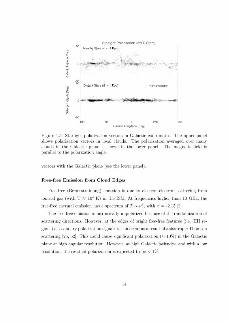
Figure 1.5: Starlight polarization vectors in Galactic coordinates. The upper panelshows polarization vectors in local clouds. The polarization averaged over manyclouds in the Galactic plane is shown in the lower panel. The magnetic field isparallel to the polarization angle.
vectors with the Galactic plane (see the lower panel).
Free-free Emission from Cloud Edges
Free-free (Bremsstrahlung) emission is due to electron-electron scattering from
ionized gas (with T ≈ 104 K) in the ISM. At frequencies higher than 10 GHz, the
free-free thermal emission has a spectrum of T ∼ νβ , with β = -2.15 [2].
The free-free emission is intrinsically unpolarized because of the randomization of
scattering directions. However, at the edges of bright free-free features (i.e. HII re-
gions) a secondary polarization signature can occur as a result of anisotropic Thomson
scattering [25, 52]. This could cause significant polarization (≈ 10%) in the Galactic
plane at high angular resolution. However, at high Galactic latitudes, and with a low
resolution, the residual polarization is expected to be < 1%.
14
1.4.4 Anomalous Dust Emission
There are additional dust emission mechanisms that could produce a low level
of polarized emission. Some studies at high Galactic latitude [53, 54, 55, 56] and
individual Galactic clouds [57, 58], have observed unexpected emission in excess of
that from the three components discussed above (synchrotron, thermal dust, and free-
free emission). This emission has been termed “anomalous” for the reason that its
provenance was not completely understood at this time. Some studies [57, 59, 60, 61]
show that this emission is correlated with large-scale maps of far infrared emission
from thermal dust.
There are two main hypotheses for the anomalous emission. The first mechanism
is the spinning dust model: small (≈ 1 nm), rapidly rotating dust grains emit electric
dipole radiation at microwave frequencies [62, 63, 64]. The second is the vibrat-
ing magnetic dust model: large (≥ 100 nm), thermally vibrating grains undergoing
fluctuations in their magnetization will emit magnetic dipole radiation at microwave
frequencies [65].
The spinning dust model is favored by some observations [66, 67]. However, emis-
sion from vibrating magnetic dust should exist at some level, because large grains are
known to exist from observed emission in the far infrared, and contain ferromagnetic
material [68, 69]. This is important for polarization observations as magnetic dust is
predicted to be better aligned to the magnetic fields than the spinning dust.
The spinning dusts aligned by paramagnetic dissipation [28] emit polarized radi-
ation. Theory predicts the polarization from spinning dust peaks at about 2 GHz
(≈ 7%) and falls below 0.5% above 30 GHz [70]. Observations [71, 72] suggest that
the spinning dust grains are inefficiently aligned and will produce little polarization at
any frequency. There is evidence that the vibrating magnetic grains are well aligned
with the magnetic field. Theory predicts a maximum polarization fraction to be 40%
[65] with the polarization angle flipping within the ∼ 1 - 100 GHz range. The po-
larization is perpendicular to the magnetic field at higher frequencies, but parallel to
the field at lower frequencies.
15
Chapter 2
Submillimeter Polarimetry of M17
In this chapter, I present the data analysis process of 450 µm polarization observa-
tions of the M17 molecular cloud from the Caltech Submillimeter Observatory (CSO)
and discuss the physics of the cloud that we learn from the submillimeter polarimetry.
2.1 Introduction to Submillimter Polarimetry
Although it is possible to measure polarized thermal emission of aligned grains
from mid-IR to millimeter wavelengths [73, 23], for a blackbody spectrum, the peak
of the thermal emission spectrum of a typical molecular cloud (with a temperature
of about 10 K [74]) falls in the submillimeter band (see appendix B). Thus, the
submillimeter waveband is a very important window for studying the physics of these
interstellar medium.
Submillimeter polarimetry provides one of the best methods for mapping interstel-
lar magnetic fields in star forming regions and other interstellar clouds [75]. Magnetic
fields are believed to play an important role in the support and evolution of molecular
clouds via the magnetic flux freezing effect [76].
The way in which polarization data traces the magnetic field is described in sec-
tion 1.4.2. Basically, the magnetically aligned interstellar dust grains emit partially
polarized thermal radiation. The direction of polarization gives the orientation of the
interstellar magnetic field, as projected onto the plane of the sky (B⊥).
16
2.2 Polarimetry at Caltech Submillimeter Obser-
vatory
The earliest detections of far-IR/submillimeter polarization in astronomical ob-
jects were obtained during the 1980s using single-pixel polarimeters from balloons [77]
and aircraft [78]. In the 1990s, astronomers developed more powerful polarimeters
with tens of pixels, such as Stokes [79] for the Kuiper Airborne Observatory (KAO),
SCU-POL [80, 81] for the James Clerk Maxwell Telescope (JCMT) and Hertz [82] for
the CSO. Since 2006, SHARP [83] has served as a new polarimeter for the CSO.
The CSO is one of the world’s premier submillimeter telescopes on Mauna Kea.
It consists of a 10.4 meter diameter dish with a root-mean-square (rms) surface error
of about 20 µm [84] and an active optics system [85]. The superconductor-insulator-
superconductor (SIS) receivers [86] of the CSO are available from 180 to 720 GHz
atmospheric windows with the performance close to the theoretical limit given by
“Quantum Noise” [87].
Submillimeter High Angular Resolution Camera II (SHARC II) [88] is a background-
limited “CCD-style” bolometer array with 12 × 32 semiconducting bolometric detec-
tors. As a facility camera for the CSO, SHARC II operates at 350 µm and 450 µm
wavebands. In the best 25% of winter nights on Mauna Kea (with τ225 GHz ≈ 0.05),
SHARC II is expected to have a noise equivalent flux density (NEFD 1) at 350 µm
of 1 Jy s1/2 or better (equation 2.1 [3] and figure 2.1).
NEFD350 µm = 1.0× exp(25.0× τ225 GHz × airmass− 1.6) Jy s1/2. (2.1)
SHARP [4] is a foreoptics module that converts the SHARC II camera into a
sensitive dual-beam 12 × 12 pixel imaging polarimeter at wavelengths of 350 and
450 µm. It splits the incident radiation into two orthogonally polarized beams that
are then reimaged onto 12 × 12 subarrays at opposite ends of the 32 ×12 array in
SHARC II. The polarization signal is modulated by a warm rotating half wave plate
(HWP) at front of the polarization-splitting optics.
1NEFD is defined as the level of flux density required to obtain a unity signal to noise ratio in 1
17
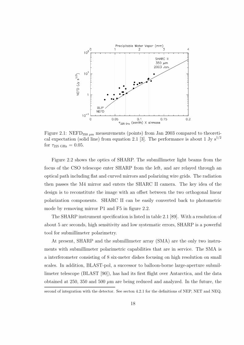
Figure 2.1: NEFD350 µm measurements (points) from Jan 2003 compared to theoreti-cal expectation (solid line) from equation 2.1 [3]. The performance is about 1 Jy s1/2
for τ225 GHz = 0.05.
Figure 2.2 shows the optics of SHARP. The submillimeter light beams from the
focus of the CSO telescope enter SHARP from the left, and are relayed through an
optical path including flat and curved mirrors and polarizing wire grids. The radiation
then passes the M4 mirror and enters the SHARC II camera. The key idea of the
design is to reconstitute the image with an offset between the two orthogonal linear
polarization components. SHARC II can be easily converted back to photometric
mode by removing mirror P1 and F5 in figure 2.2.
The SHARP instrument specification is listed in table 2.1 [89]. With a resolution of
about 5 arc seconds, high sensitivity and low systematic errors, SHARP is a powerful
tool for submillimeter polarimetry.
At present, SHARP and the submillimeter array (SMA) are the only two instru-
ments with submillimeter polarimetric capabilities that are in service. The SMA is
a interferometer consisting of 8 six-meter dishes focusing on high resolution on small
scales. In addition, BLAST-pol, a successor to balloon-borne large-aperture submil-
limeter telescope (BLAST [90]), has had its first flight over Antarctica, and the data
obtained at 250, 350 and 500 µm are being reduced and analyzed. In the future, the
second of integration with the detector. See secton 4.2.1 for the definitions of NEP, NET and NEQ.
18
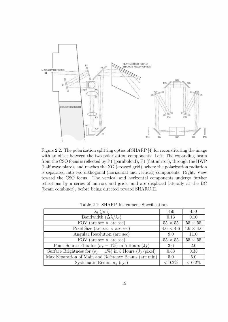
Figure 2.2: The polarization splitting optics of SHARP [4] for reconstituting the imagewith an offset between the two polarization components. Left: The expanding beamfrom the CSO focus is reflected by P1 (paraboloid), F1 (flat mirror), through the HWP(half wave plate), and reaches the XG (crossed grid), where the polarization radiationis separated into two orthogonal (horizontal and vertical) components. Right: Viewtoward the CSO focus. The vertical and horizontal components undergo furtherreflections by a series of mirrors and grids, and are displaced laterally at the BC(beam combiner), before being directed toward SHARC II.
Table 2.1: SHARP Instrument Specifications
λ0 (µm) 350 450Bandwidth (∆λ/λ0) 0.13 0.10
FOV (arc sec × arc sec) 55 × 55 55 × 55Pixel Size (arc sec × arc sec) 4.6 × 4.6 4.6 × 4.6Angular Resolution (arc sec) 9.0 11.0FOV (arc sec × arc sec) 55 × 55 55 × 55
Point Source Flux for (σp = 1%) in 5 Hours (Jy) 3.6 2.0Surface Brightness for (σp = 1%) in 5 Hours (Jy/pixel) 0.63 0.35Max Separation of Main and Reference Beams (arc min) 5.0 5.0
Systematic Errors, σp (sys) < 0.2% < 0.2%
19
I
Q
U
R
A
W
rgm H/V
Gain
De-
modula!on
Chopped
Data
C
Figure 2.3: Flow chart of “SharpInteg”. It starts by masking the raw data file with an“rgm” file. Then, it demodulates the chopping to calculate the chopped data. Afterapplying the relative data gain factor between the horizontal and vertical array, itcalculates the I, I-error, Q, Q-error, U and U-error components and saves them intoa new file.
SCUBA-2 [91] instrument being commissioned at the JCMT also has a polarimeter,
POL-2, and the ALMA interferometer should also have polarimetric capabilities at
multiple submillimeter/millimeter wavelengths.
2.3 SHARP Data Pipeline
There are two data processing programs for SHARP pipeline: “SharpInteg” and
“Sharpcombine”. “SharpInteg” is a program that takes a cycle of half wave plate mea-
surement from SHARP and process it to for I, Q and U along with the corresponding
errors. “Sharpcombine” is for map combining and smoothing.
As shown in figure 2.3, “SharpInteg” first reads in the SHARC II raw data file and
apply a pixel mask to it from a pixel mask file (“rgm” file). After that, the chopping is
demodulated, and the data at different chop/nod positions is given a weight equals to
the number of samples at that position. The chopped data is calculated by summing
the weighted raw data within each sampling period. In the next step, the relative data
20
I
Q
U
I
Q
U
I
Q
U
B
S
I
Q
U
I
Q
U
I.P.
S
I
Q
U Rot
I
Q
U
I
Q
U
I
Q
U
B
S
I
Q
U
I
Q
U
I.P.
S
I
Q
U Rot
I
Q
U
I
Q
U
I
Q
U
B
S
I
Q
U
I
Q
U
I.P.
S
I
Q
U Rot
I
Q
U
I
Q
U
III
Q
U
UU
Figure 2.4: Flow chart of “Sharpcombine”. It applies τ and telescope pointing cor-rection, background subtraction (BS), instrument polarization (I.P.) subtraction andpolarization angle rotation to sky coordinates (Rot) to each sub-map before it com-bines them into a large map and smooths it.
gain factor (f) between the horizontal (“H”) and vertical (“V”) array is calculated by
taking all of the samples from a particular HWP position and fitting to the line of “V
= a H + b” using numerical method. After this is done for all HWP positions, the
median value is taken and f is set to the inverse value of the median. The “H” and
“V” array samples are combined after calculating the f value. Finally, The I, I-error,
Q, Q-error, U and U-error maps are calculated and saved to a FITS file.
“Sharpcombine” starts with the output FITS files from “SharpInteg” containing
the I, Q and U map. Each of them represents a small map to be combined to a large
map. In the first step, it applies τ (atmospheric optical depth) and telescope pointing
21
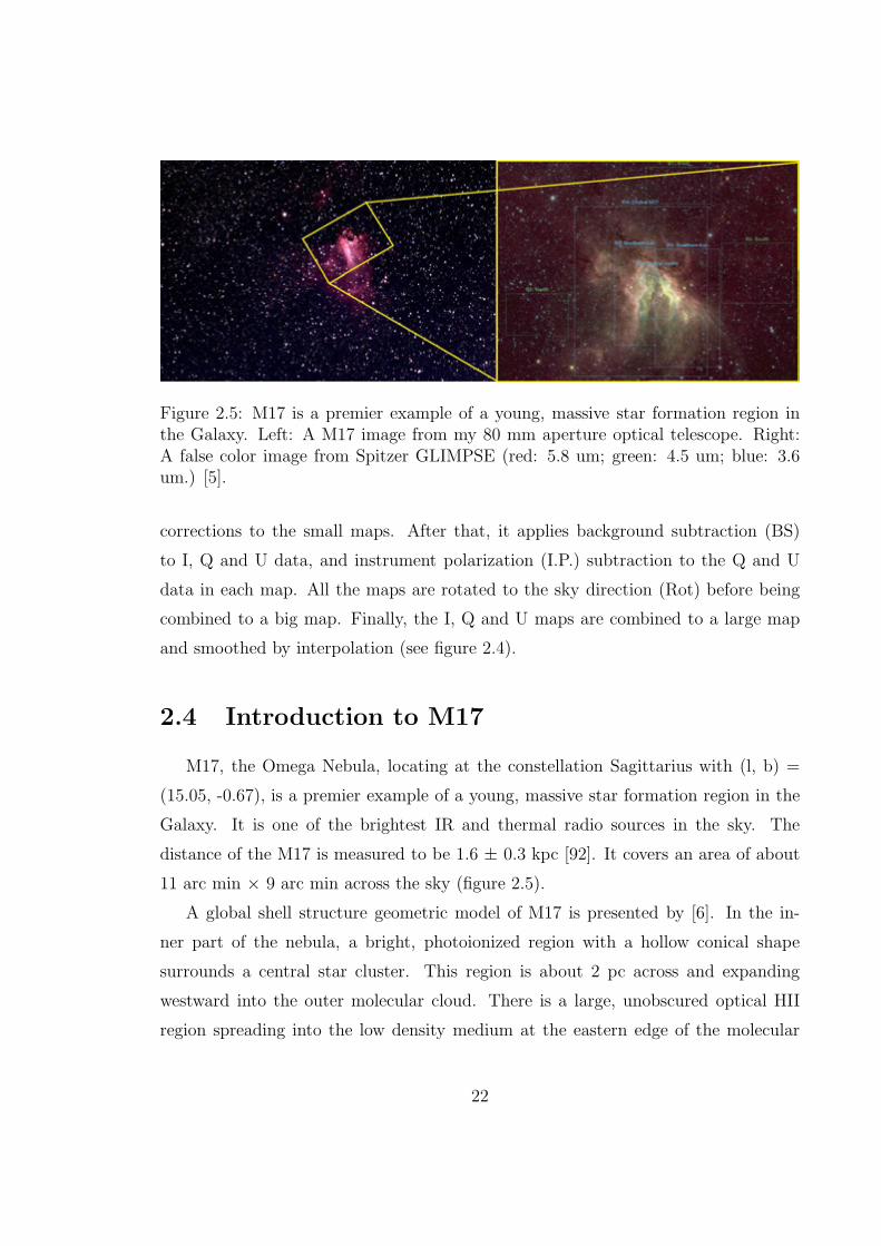
Figure 2.5: M17 is a premier example of a young, massive star formation region inthe Galaxy. Left: A M17 image from my 80 mm aperture optical telescope. Right:A false color image from Spitzer GLIMPSE (red: 5.8 um; green: 4.5 um; blue: 3.6um.) [5].
corrections to the small maps. After that, it applies background subtraction (BS)
to I, Q and U data, and instrument polarization (I.P.) subtraction to the Q and U
data in each map. All the maps are rotated to the sky direction (Rot) before being
combined to a big map. Finally, the I, Q and U maps are combined to a large map
and smoothed by interpolation (see figure 2.4).
2.4 Introduction to M17
M17, the Omega Nebula, locating at the constellation Sagittarius with (l, b) =
(15.05, -0.67), is a premier example of a young, massive star formation region in the
Galaxy. It is one of the brightest IR and thermal radio sources in the sky. The
distance of the M17 is measured to be 1.6 ± 0.3 kpc [92]. It covers an area of about
11 arc min × 9 arc min across the sky (figure 2.5).
A global shell structure geometric model of M17 is presented by [6]. In the in-
ner part of the nebula, a bright, photoionized region with a hollow conical shape
surrounds a central star cluster. This region is about 2 pc across and expanding
westward into the outer molecular cloud. There is a large, unobscured optical HII
region spreading into the low density medium at the eastern edge of the molecular
22
cloud. Gas photoexcited by the early OB stars is concentrated in the northern and
southern bars.
X-ray observations [93, 94] indicate that the region interior to the HII region is
filled by hot (106 - 107 K) gas, which is flowing out to the east. [93] noted that this
region is too young to have produced a supernova remnant and interpret the X-ray
emission as hot gas filling a super bubble blown by the OB star winds. In the middle
of the nebula, velocity studies show an ionized shell with a diameter of about 6 pc.
On the western side of the outer part, all tracers of warm and hot gas are truncated
by a wall of dense, cold molecular material which includes the dense cores known
as “M17 Southwest” and “M17 North”, which exhibit many other tracers of current
massive star formation. At this region, Only the most massive members of the young
NGC6618 stellar cluster [95] exciting the nebula have been characterized, due to the
comparatively high extinction.
Figure 2.6 shows a simple M17 model. We can represent the system as a central
cluster of stars surrounded by successive layers of H+, H0, and H2 gas to the SW side
and by a background sheet of ionized and neutral gas wrapping around to the NE.
2.5 M17 Polarimetry Results
2.5.1 General Results
Our M17 map from the SHARP 450 µm observation, is centered at 18h17m32.0s,
−1614′25.0′′ (B1950) or 18h20m25.2s, −1613′02.1′′ (J2000). It covers an area of
about 4′25′′ × 2′45′′ at the SW bar of M17 (figure 2.10). Taking the distance to M17
to be about 1.6 kpc (section 2.4), our map coverage is equivalent to an area of 2.05
pc × 1.28 pc.
M17 polarization vectors are plotted in figure 2.7 and a table of the vectors is
listed in appendix A.5. As we can see in figure 2.7, for regions of high submillimeter
flux, the average polarization fraction is lower than that in low flux regions. This is
caused by the line of sight (LOS) effect: assuming the polarization angles at different
distances along the los to be variable, the measured polarization fraction trends to
23
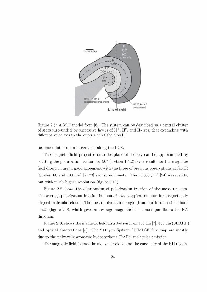
Figure 2.6: A M17 model from [6]. The system can be described as a central clusterof stars surrounded by successive layers of H+, H0, and H2 gas, that expanding withdifferent velocities to the outer side of the cloud.
become diluted upon integration along the LOS.
The magnetic field projected onto the plane of the sky can be approximated by
rotating the polarization vectors by 90 (section 1.4.2). Our results for the magnetic
field direction are in good agreement with the those of previous observations at far-IR
(Stokes, 60 and 100 µm) [7, 23] and submillimeter (Hertz, 350 µm) [24] wavebands,
but with much higher resolution (figure 2.10).
Figure 2.8 shows the distribution of polarization fraction of the measurements.
The average polarization fraction is about 2.4%, a typical number for magnetically
aligned molecular clouds. The mean polarization angle (from north to east) is about
−5.0 (figure 2.9), which gives an average magnetic field almost parallel to the RA
direction.
Figure 2.10 shows the magnetic field distribution from 100 um [7], 450 um (SHARP)
and optical observations [8]. The 8.00 µm Spitzer GLIMPSE flux map are mostly
due to the polycyclic aromatic hydrocarbons (PAHs) molecular emission.
The magnetic field follows the molecular cloud and the curvature of the HII region.
24
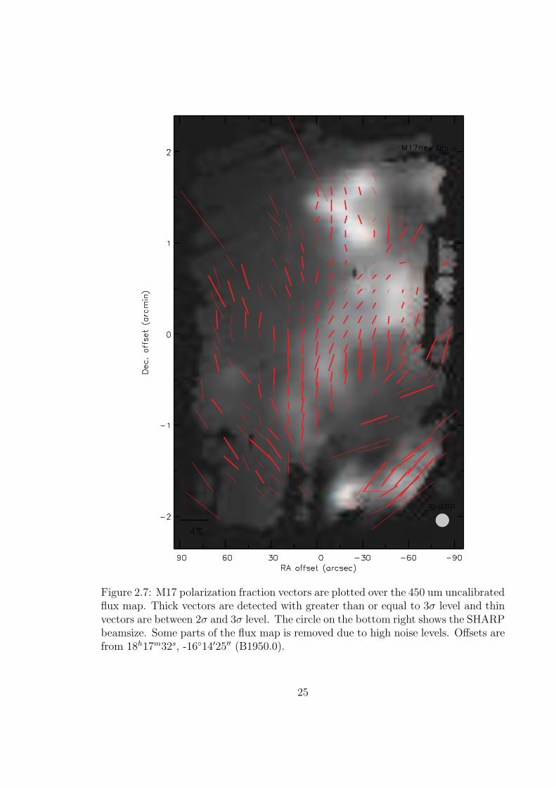
Figure 2.7: M17 polarization fraction vectors are plotted over the 450 um uncalibratedflux map. Thick vectors are detected with greater than or equal to 3σ level and thinvectors are between 2σ and 3σ level. The circle on the bottom right shows the SHARPbeamsize. Some parts of the flux map is removed due to high noise levels. Offsets arefrom 18h17m32s, -1614′25′′ (B1950.0).
25
0 1 2 3 4 5 6 7 8 9 10 11 12 13 14 15 16Polarization (%)
0
10
20
30
40
50
60
70
80
Num
ber
Median = 1.90, Mean = 2.36, Std = 1.81
Figure 2.8: Histogram of M17 polarization fraction. This distribution includes allvectors at greater or equal to than 2σ level. All vectors greater than 10% are 2σvectors.
908070605040302010 0 10 20 30 40 50 60 70 80Polarization Angle (degree)
0
5
10
15
20
25
30
35
40
Num
ber
Median = -4.00, Mean = -5.02, Std = 30.39
Figure 2.9: Histogram of M17 polarization angle. Polarization angles are measuredfrom north to east. The resulting net magnetic field is almost parallel to the RAdirection.
26
The center OB type stars heat the HII region and carve a hollow conical shape into
the molecular cloud and separating it into two parts: the M17 SW and the M17 N.
It is found that PAHs are destroyed over a short distance at the photodissociation
region (PDR) around the edge of the HII bubble [5].
2.5.2 Polarization Spectrum
There are several instruments that contribute multiwavelength polarimetric data
from far-IR (Stokes) to submillimeter (Hertz, SHARP, SCU-POL). If the source of
the polarized emission is a single population of dust grains with similar polariza-
tion properties and temperature, then one expects the magnitude of the polarization
(polarization fraction) to be nearly independent of wavelength higher than 50 µm
[96, 97].
The far-IR to submillimeter polarization spectrum of various molecular clouds
have been studied by observations [97, 98, 99, 100] and simulations [101, 102]. The
polarization spectrum of M17 at 60 um (Stokes, 22′′ resolution), 100 um (Stokes, 35′′
resolution) and 350 um (Hertz, 20′′ resolution) had been studied by [97, 98] and their
results are shown in figure 2.12. It has been found that the spectra are falling from
far-IR to about 350 µm and rising towards longer wavelengths.
The analysis presented here incorporate the 450 µm SHARP polarimetric data
(about 10′′ resolution). The polarization data points that are to be compared between
two wavelengths are chosen based on the following criteria [97]: (1) The vectors are in
the same region of the same cloud; (2) The difference between the polarization angle
must be within 10; (3) The vectors are from the cloud envelope; (4) All vectors are
greater or equal to 3σ level.
Applying the above criterion, the surviving vectors at 60 µm to 450 µm are plotted
in figure 2.11. They share a common area (marked by a green shadow) between
18h17m30s and 18h17m37s in Ra (B1950), −1616′20′′ and −1613′00′′ in Dec (B1950).
A summary of the result is presented in table 2.2 and the details can be found
in appendix A. The M17 polarization spectrum from 60 µm to 450 µm is plotted
in figure 2.12. Our basic result is P450 < P350 < P100 < P60. In contrast to the
27
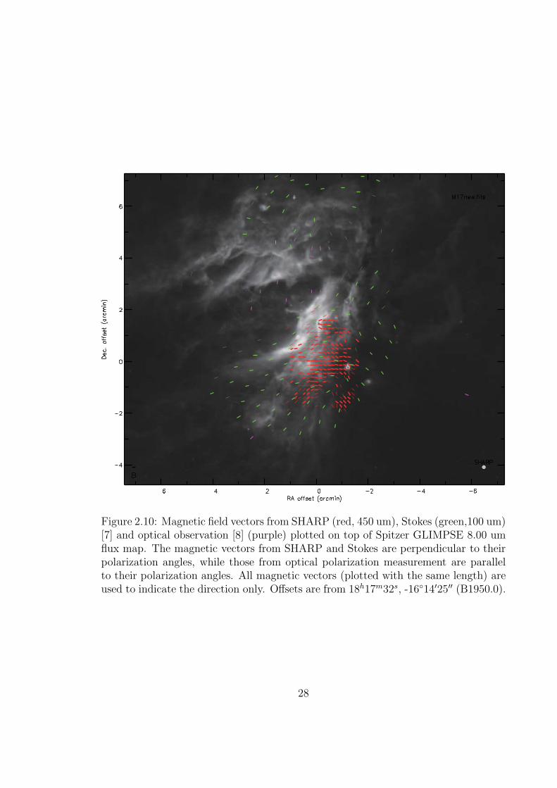
Figure 2.10: Magnetic field vectors from SHARP (red, 450 um), Stokes (green,100 um)[7] and optical observation [8] (purple) plotted on top of Spitzer GLIMPSE 8.00 umflux map. The magnetic vectors from SHARP and Stokes are perpendicular to theirpolarization angles, while those from optical polarization measurement are parallelto their polarization angles. All magnetic vectors (plotted with the same length) areused to indicate the direction only. Offsets are from 18h17m32s, -1614′25′′ (B1950.0).
28
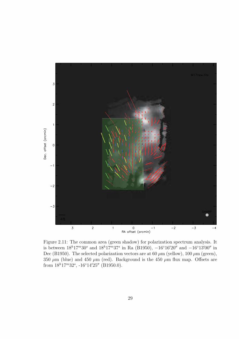
Figure 2.11: The common area (green shadow) for polarization spectrum analysis. Itis between 18h17m30s and 18h17m37s in Ra (B1950), −1616′20′′ and −1613′00′′ inDec (B1950). The selected polarization vectors are at 60 µm (yellow), 100 µm (green),350 µm (blue) and 450 µm (red). Background is the 450 µm flux map. Offsets arefrom 18h17m32s, -1614′25′′ (B1950.0).
29
Table 2.2: M17 Polarization Spectrum Data
Ratio Points Median Mean Std NoteP450/P60 13 0.390 0.395 0.056 see appendix A.1 for detailsP450/P100 11 0.520 0.525 0.128 see appendix A.2 for detailsP450/P350 22 0.795 0.887 0.289 see appendix A.3 for details
results from other clouds, our work shows that, in the common area, the M17 has
lower median polarization at 450 µm than at 350 µm. The polarization spectrum
falls monotonically from 60 µm to 450 µm.
There are many models to explain the rising (or falling) of the polarization spec-
trum from far-IR to submillimeter wavelength. Generally speaking, the radiation
environment plays an important role in forming the polarization spectrum, since the
grain alignment efficiency is dependent on radiative torques (section 1.4.2). In a weak
radiation field, the polarization spectrum normally has a positive slope (towards long
wavelengths) [101]. That is what we observed from many clouds from 350 µm to 450
µm (figure 2.12). Our result of a negative slope (P450 < P350) from the east part of
the cloud indicates the existence of a strong radiation field from that direction.
2.5.3 Spatial Distribution of Magnetic Field and Polarization
Spectrum
As already shown in figure 2.10, the center OB type stars in M17 heat the HII
region and carve a hollow conical shape into the molecular cloud. Our analysis shows
that this shock front is passing through our sampled region. Figure 2.13 shows 450
µm magnetic vectors plotted over the [21 cm]/[450 µm] ratio map (with the peak
normalized to 1.0). The shock is following the “-Y” direction. We can separate the
cloud into three regions: “post-shocked”, “shock front” and “pre-shocked” by the “y
= 0” and “y = -50 arcsec” lines.
The “post-shocked” region has consistent polarization angles with an average of
about 18; in the “shock front” region, where the magnetic field is being distorted, the
30
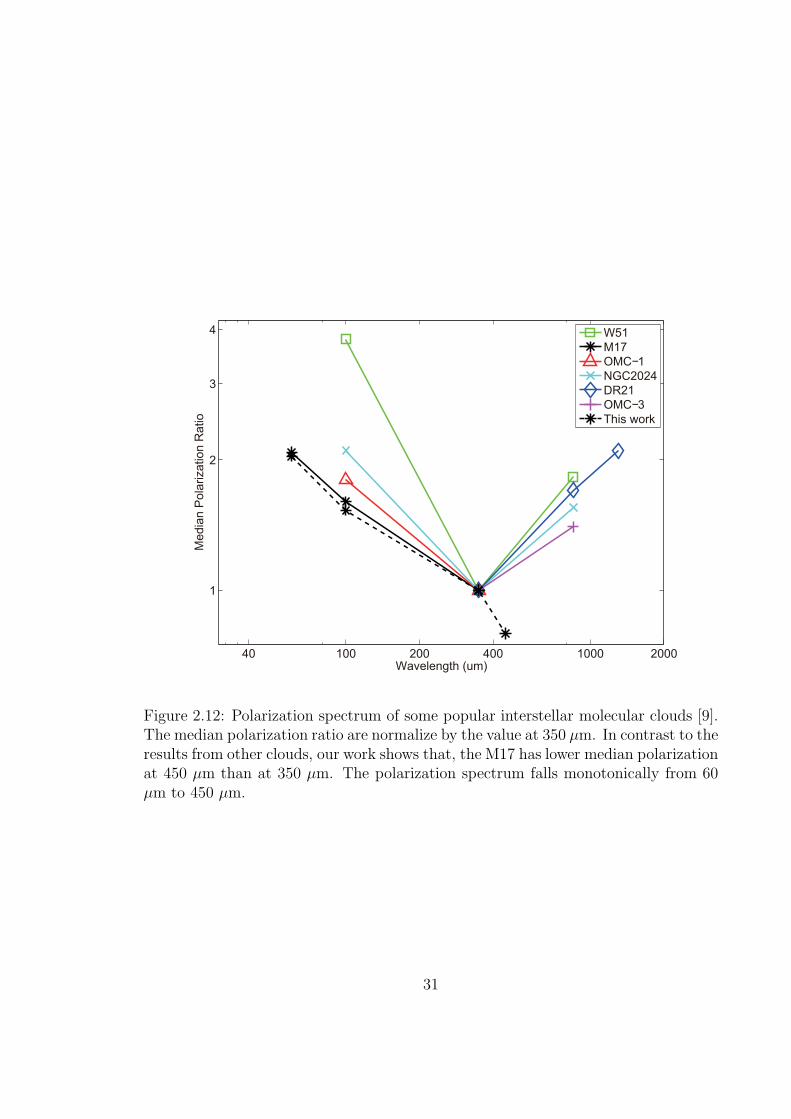
40 100 200 400 1000 2000
1
2
3
4
Wavelength (um)
Med
ian
Pol
ariz
atio
n R
atio
W51M17OMC−1NGC2024DR21OMC−3This work
Figure 2.12: Polarization spectrum of some popular interstellar molecular clouds [9].The median polarization ratio are normalize by the value at 350 µm. In contrast to theresults from other clouds, our work shows that, the M17 has lower median polarizationat 450 µm than at 350 µm. The polarization spectrum falls monotonically from 60µm to 450 µm.
31
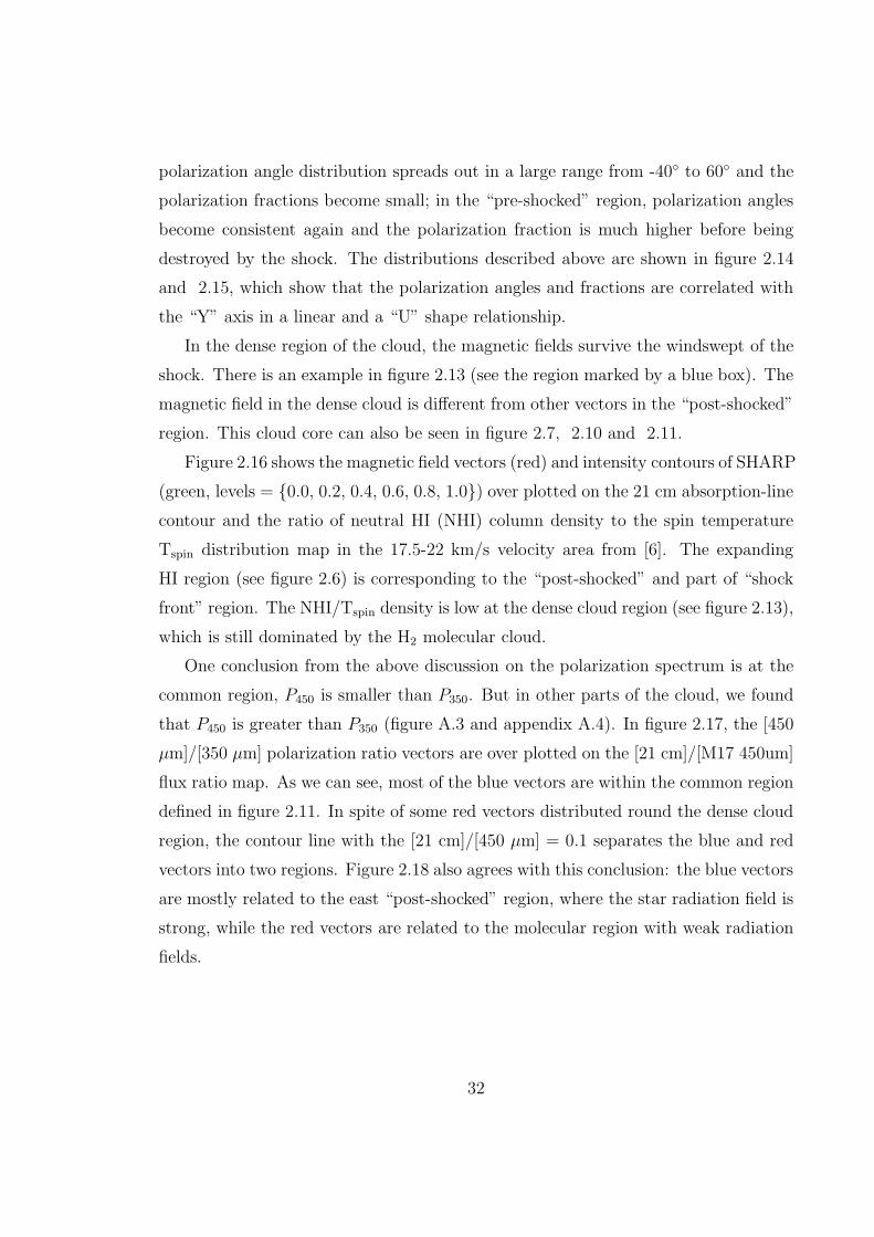
polarization angle distribution spreads out in a large range from -40 to 60 and the
polarization fractions become small; in the “pre-shocked” region, polarization angles
become consistent again and the polarization fraction is much higher before being
destroyed by the shock. The distributions described above are shown in figure 2.14
and 2.15, which show that the polarization angles and fractions are correlated with
the “Y” axis in a linear and a “U” shape relationship.
In the dense region of the cloud, the magnetic fields survive the windswept of the
shock. There is an example in figure 2.13 (see the region marked by a blue box). The
magnetic field in the dense cloud is different from other vectors in the “post-shocked”
region. This cloud core can also be seen in figure 2.7, 2.10 and 2.11.
Figure 2.16 shows the magnetic field vectors (red) and intensity contours of SHARP
(green, levels = 0.0, 0.2, 0.4, 0.6, 0.8, 1.0) over plotted on the 21 cm absorption-line
contour and the ratio of neutral HI (NHI) column density to the spin temperature
Tspin distribution map in the 17.5-22 km/s velocity area from [6]. The expanding
HI region (see figure 2.6) is corresponding to the “post-shocked” and part of “shock
front” region. The NHI/Tspin density is low at the dense cloud region (see figure 2.13),
which is still dominated by the H2 molecular cloud.
One conclusion from the above discussion on the polarization spectrum is at the
common region, P450 is smaller than P350. But in other parts of the cloud, we found
that P450 is greater than P350 (figure A.3 and appendix A.4). In figure 2.17, the [450
µm]/[350 µm] polarization ratio vectors are over plotted on the [21 cm]/[M17 450um]
flux ratio map. As we can see, most of the blue vectors are within the common region
defined in figure 2.11. In spite of some red vectors distributed round the dense cloud
region, the contour line with the [21 cm]/[450 µm] = 0.1 separates the blue and red
vectors into two regions. Figure 2.18 also agrees with this conclusion: the blue vectors
are mostly related to the east “post-shocked” region, where the star radiation field is
strong, while the red vectors are related to the molecular region with weak radiation
fields.
32
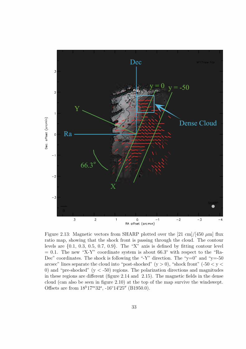
Y
X
Dec
Ra
66.3o
y = 0 y = -50
Dense Cloud
Figure 2.13: Magnetic vectors from SHARP plotted over the [21 cm]/[450 µm] fluxratio map, showing that the shock front is passing through the cloud. The contourlevels are 0.1, 0.3, 0.5, 0.7, 0.9. The “X” axis is defined by fitting contour level= 0.1. The new “X-Y” coordinate system is about 66.3 with respect to the “Ra-Dec” coordinates. The shock is following the “-Y” direction. The “y=0” and “y=-50arcsec” lines separate the cloud into “post-shocked” (y > 0), “shock front” (-50 < y <0) and “pre-shocked” (y < -50) regions. The polarization directions and magnitudesin these regions are different (figure 2.14 and 2.15). The magnetic fields in the densecloud (can also be seen in figure 2.10) at the top of the map survive the windswept.Offsets are from 18h17m32s, -1614′25′′ (B1950.0).
33
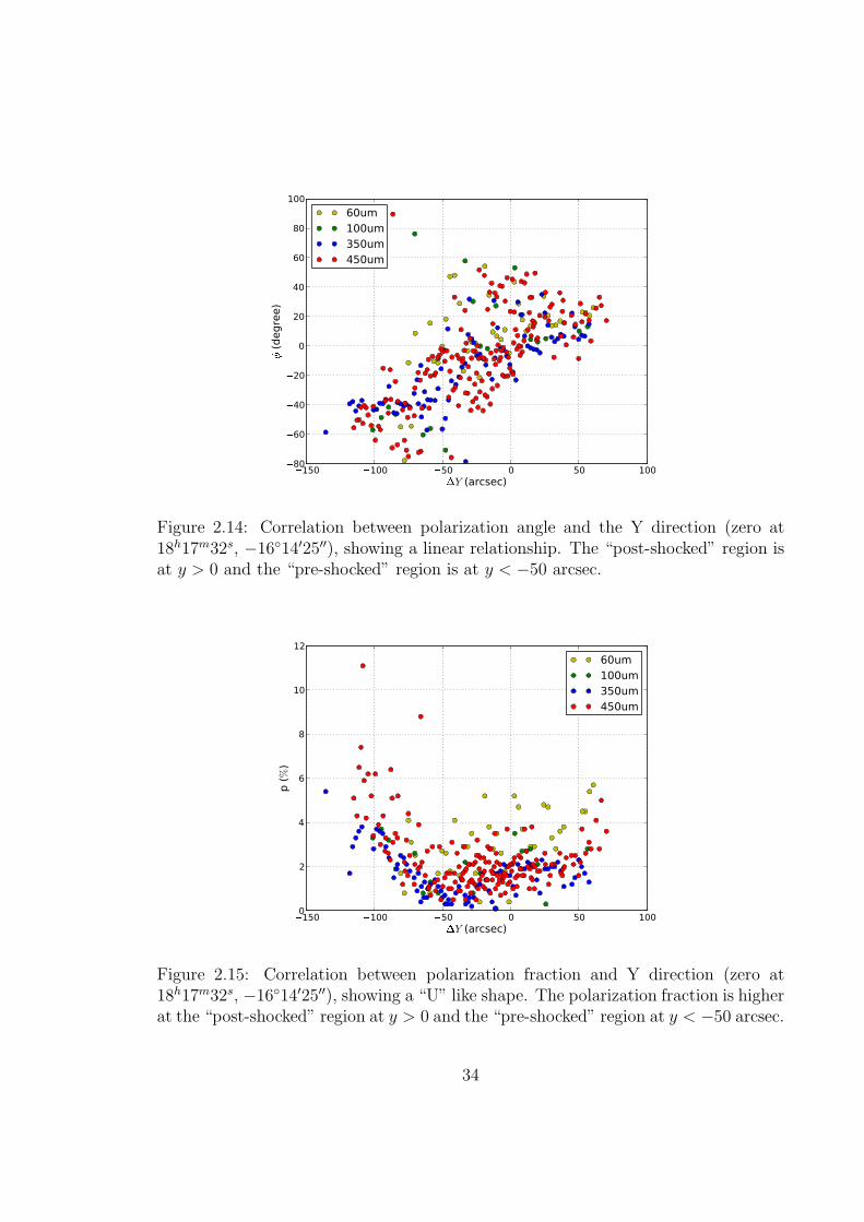
150 100 50 0 50 100Y (arcsec)
80
60
40
20
0
20
40
60
80
100
(deg
ree)
60um100um350um450um
Figure 2.14: Correlation between polarization angle and the Y direction (zero at18h17m32s, −1614′25′′), showing a linear relationship. The “post-shocked” region isat y > 0 and the “pre-shocked” region is at y < −50 arcsec.
150 100 50 0 50 100Y (arcsec)
0
2
4
6
8
10
12
p (%
)
60um100um350um450um
Figure 2.15: Correlation between polarization fraction and Y direction (zero at18h17m32s, −1614′25′′), showing a “U” like shape. The polarization fraction is higherat the “post-shocked” region at y > 0 and the “pre-shocked” region at y < −50 arcsec.
34
Figure 2.16: Magnetic field vectors (red) and intensity contours of SHARP (green,levels = 0.0, 0.2, 0.4, 0.6, 0.8, 1.0) are over plotted on the 21 cm absorption-linecontour and the ratio of neutral HI (NHI) column density to the spin temperatureTspin distribution map in the 17.5-22 km/s velocity area from [6]. This velocitycomponent is correlated with the “post-shocked” and part of “shock front” region.The NHI/Tspin density at the dense cloud region (see figure 2.13) is low.
35
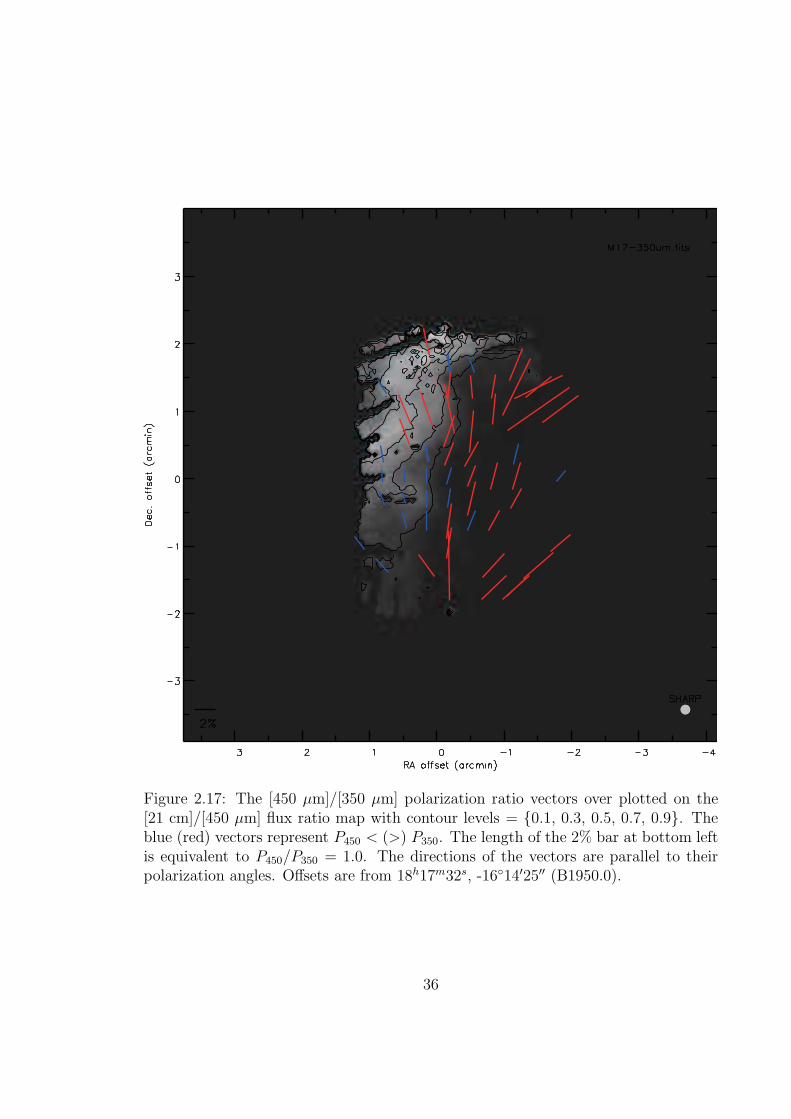
Figure 2.17: The [450 µm]/[350 µm] polarization ratio vectors over plotted on the[21 cm]/[450 µm] flux ratio map with contour levels = 0.1, 0.3, 0.5, 0.7, 0.9. Theblue (red) vectors represent P450 < (>) P350. The length of the 2% bar at bottom leftis equivalent to P450/P350 = 1.0. The directions of the vectors are parallel to theirpolarization angles. Offsets are from 18h17m32s, -1614′25′′ (B1950.0).
36
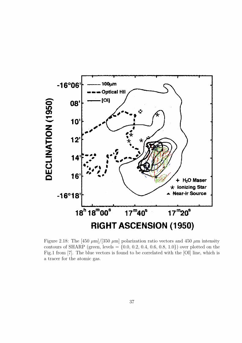
Figure 2.18: The [450 µm]/[350 µm] polarization ratio vectors and 450 µm intensitycontours of SHARP (green, levels = 0.0, 0.2, 0.4, 0.6, 0.8, 1.0) over plotted on theFig.1 from [7]. The blue vectors is found to be correlated with the [OI] line, which isa tracer for the atomic gas.
37
2.5.4 Conclusion
The combination of multi wavelength study and the polarimetric data from far-IR
to submillimeter reveal the violent physical process in the M17 cloud.
At large scale, the young OB type stars in the center of the cloud heat the HII
region up to 106 - 107 K and create a high energy fountain towards the southeast
direction. The HII wind push the HI and H2 regions outwards, creating a hollow
conical shape into the cloud. The magnetic field is found following the curve of the
HII region.
On small scales, within our field of view, the shock is passing through the boundary
between the HI and H2 region. There are significant differences between the dust
alignment before and after the shock. The polarization properties and temperature
of the dust population are also changed by the wind. Our study also shows that a high
density molecular clump is being blasted by the out-going wind, while the magnetic
field distribution in the area remains unchanged.
It is the first time to observe the variance of polarization ratios across a molecular
cloud. There are still no models that can explain this result. One conclusion we can
make is that the grains in the cloud are not always aligned with the magnetic field
perfectly, and any model trying to explain the polarization spectrum should take into
account the variance of interstellar physical condition along the line of sight.
38
Part II
Polarimetry in Cosmology
39
Chapter 3
Introduction to Polarization in
Cosmology
3.1 The Big Bang Theory
The Big Bang theory describes the evolution of our universe. It posits that our
universe started from a hot and dense phase about 13.75 billion years [14] ago and
the content of the universe kept evolving after that. In inflation theory, the universe
was dominated by an energy field with a negative pressure, which drove an early
period of accelerated expansion. It was then dominated by radiation, and later by
matter. And now, it has again become dominated by a dark energy that is driving a
slower accelerated expansion (equation 3.27). The term “Big Bang” was first coined
by Fred Hoyle, when he was trying to belittle the credibility of the theory. However,
The Big Bang has became the standard cosmological framework for understanding
the universe and is supported by many lines of evidence.
3.1.1 The Expanding Universe–Hubble’s Law
In 1929, Edwin Hubble announced his discovery (now Hubble’s Law) [103], that
describes the relation between radial velocity (V ) and distance (D) of extra-Galactic
40
“nebulae” (galaxies):
V = H0D (3.1)
where H0 is Hubble constant.
Hubble’s law basically describes that the more distant the galaxy, the faster it is
receding from us and galaxies are moving away from each other. It is the result that
we expect for a uniformly expanding universe.
3.1.2 Big Bang Nucleosynthesis (BBN)
At the time of about 3 minutes after the Big Bang, the universe is hot and dense.
There were no atomic elements, but rather a sea of neutrons, protons, electrons,
positrons, photons and neutrinos. As the universe cooled, the following processes
occurred:
n→ p+ + e− + νe n+ p+ →21 D+ γ
21D + p+ →3
2 He + γ 21D +2
1 D →42 He + γ
21D+2
1 D →31 T+ p+ 2
1D +31 T →4
2 He + n
... ... (3.2)
This process of light element formation in the early universe is called “Big Bang
nucleosynthesis” (BBN). It lasted for only about 17 minutes. After that, the limited
lifetime of free neutrons ended the process, while the temperature and density of
the universe fell below that which is required for nuclear fusion. The brevity of
BBN is important because it predicts that only light elements could be form, and
the abundance of light elements are: Hydrogen(1H) ≈ 75%, Helium(4He) ≈ 25%,
Deuterium(2H) ≈ 0.01%, Helium(3H) ≈ 0.001%, Lithium(7Li) ≈ 10−10 [104, 105].
This prediction is in agreement with observations.
In 2011, pristine clouds of the primordial gas were found [106]. These clouds of gas
was discovered by analysing the light from distant quasars. Absorption lines that can
be used to measure the composition of the gas appeared in the spectrum where the
41
light was absorbed by the gas. The composition of the gas matches the predictions
from BBN, providing the latest direct evidence in support of the modern cosmological
explanation for the origins of elements in the universe.
3.1.3 The Cosmic Microwave Background (CMB) Radiation
The CMB radiation was predicted as radiation left over from an early stage in the
development of the universe (section 3.4), and its discovery is considered a landmark
success of the Big Bang theory, ruling out the competing Steady State Theory [107].
In 1964, Arno Penzias and Robert Wilson discovered the cosmic background radia-
tion while conducting diagnostic observations using a microwave receiver [108]. Their
discovery confirmed the CMB predictions from the Big Bang theory–an isotropic and
consistent blackbody spectrum with a temperature of about 3 K.
The Cosmic Background Explorer (COBE) satellite was launched in 1989. Its
findings were consistent with the Big Bang’s predictions regarding the CMB. COBE
found a precise blackbody spectrum (reflecting thermal equilibrium between matter
and radiation in the early universe) with a temperature of 2.725±0.001 K and detected
for the first time the fluctuations (anisotropy) in the CMB, at a level of about one
part in 105 [109].
In early 2003, the first results of the Wilkinson Microwave Anisotropy Probe
(WMAP) were released [11]. These results tested and refined a standard cosmological
model with accurate values for the cosmological parameters. The WMAP results were
also consistent with the inflation theory.
A new generation space probe – the Planck satellite, was launched in 2009. It has
goals similar to WMAP –to provide even more accurate measurements of the CMB
anisotropy while further testing the model. There are also many other ground- and
balloon-based experiments targeting various aspects of the CMB.
3.1.4 Other Evidence
Observations of the morphology and distribution of galaxies and quasars also
provide strong evidence for the standard model of cosmology. Observations suggest
42
that the first quasars and galaxies formed when the age of the universe was only about
0.5 billion years and distant galaxies (galaxies formed in the early universe) appear
very different from nearby galaxies (galaxies formed recently). These observations
agree well with numerical simulations [110]. The age of universe determined to < 1%
from the CMB is also in good agreement with other estimations, i.e. using the ages
of the oldest stars.
3.2 Cosmic Inflation
Cosmic inflation was originally proposed by Alan Guth [111, 112], Alexei Starobin-
sky [113], Andrei Linde [114], Andreas Albrecht and Paul Steinhardt [115]. It posits
that there was a rapid exponential expansion of the early universe by a factor of at
least 1078 in volume, driven by a negative pressure energy (ω < −1/3). Following
the grand unification epoch (between 10−43 s and 10−36 s after the Big Bang), the
inflationary epoch comprises the first part of the electroweak epoch (between 10−36 s
and 10−12 s after the Big Bang). It lasted from 10−36 s to about 10−32 s. After that,
the universe continued to expand at a rate that was much slower than inflation.
While the detailed physics mechanism responsible for inflation is still unknown,
inflation makes a number of predictions that have been confirmed by observations,
such as CMB observations, galaxy surveys and 21 cm radiation observations. Inflation
is thus now considered to be an extension of the Big Bang theory. It resolves several
problems in the Big Bang cosmology.
3.2.1 The Structure Problem
Considerable structures in the universe, from stars to galaxies to clusters and
super clusters of galaxies have been observed. How did these structures form? The
Big Bang theory does not account for the needed fluctuations to produce the structure
we see. Inflation gives a solution to this problem: Quantum fluctuations in the
nearly-uniform density of the early universe expanded to cosmic scales during cosmic
inflation. These fluctuations also would have left an imprint in the CMB radiation
43
in the form of temperature fluctuations from point to point across the sky (the CMB
anisotropy). The structures that we observe today grew from the gravitational pull
of these fluctuations.
3.2.2 The Flatness Problem
Observations show that the geometry of the current universe is nearly flat (sec-
tion 3.3.3). However, under the nominal Big Bang theory, curvature grows with time.
A universe as flat as we see it today would require an extreme fine-tuning of conditions
in the past, which would be an unbelievable coincidence. Inflation provides a solu-
tion to this problem via the stretching of any initial curvature of the 3-dimensional
universe to near flatness, resulting Ωk ≈ 0.
3.2.3 The Horizon Problem
The uniformity of the CMB temperature (section 3.4) implies that the entire
observable universe must have been in causal contact in the past. But now the
distance between two regions with ≥ 2 apart in the sky are so far apart that, they
could never have been in causal contact with each other, because the light travel
time between them is greater than the age of the universe. This can be explained by
inflation theory: Distant regions were actually much closer together prior to inflation
than they would have been with only standard Big Bang expansion. Thus, such
regions could have been in causal contact prior to inflation and could have attained
a uniform temperature.
3.2.4 The Magnetic Monopole Problem
The Big Bang theory predicts that the early universe produced a very large num-
ber of heavy and stable magnetic monopoles. However, these magnetic monopoles
have never been observed so far. The explanation from inflation is that, during in-
flation, the density of monopoles drops exponentially, so their abundance drops to
undetectable levels.
44
3.3 ΛCDM Cosmological Model
The Λ Cold Dark Matter (ΛCDM) model is a model of the content of the uni-
verse that includes baryons, cold dark matter, photons, neutrinos and a cosmological
constant Λ.
3.3.1 Cosmological Principles and FLRW metric
The cosmological principle is that, on sufficiently large scales, the universe is ho-
mogeneous and isotropic. Homogeneity implies translational invariance and isotropy
implies rotational invariance. These principles are distinct but closely related, because
a universe that appears isotropic from any two locations must also be homogeneous.
The isotropic principle is supported by the observations: (1) Radio galaxies are
randomly distributed across the sky; (2) The large scale distribution of galaxies is
isotropic in the range of greater than 200 Mpc; (3) The observed redshift distribution
of distant galaxies is isotropic, which implies a uniform expansion of space in all
directions; (4) The Cosmic Microwave Background (CMB) radiation is constant in
all directions to within 1 part in 105 (section 3.1.3).
A universe must be non-static if it follows the cosmological principle. In 1923,
Alexander Friedmann derived a version of Einstein’s equations of general relativity
describing the dynamics of a homogeneous and isotropic universe. After that, Georges
Lemaıtre, Howard P. Robertson and Arthur G. Walker also derived the general rela-
tivity metric for the cosmological principle independently. It is named Friedmann -
Lemaıtre - Robertson - Walker (FLRW) metric.
In the four space-time dimensions, using Einstein notation, the invariant is:
ds2 = gµνdxµdxν (3.3)
where the µ and ν indices range from 0 to 3.
The FLRW metric can be written as:
45
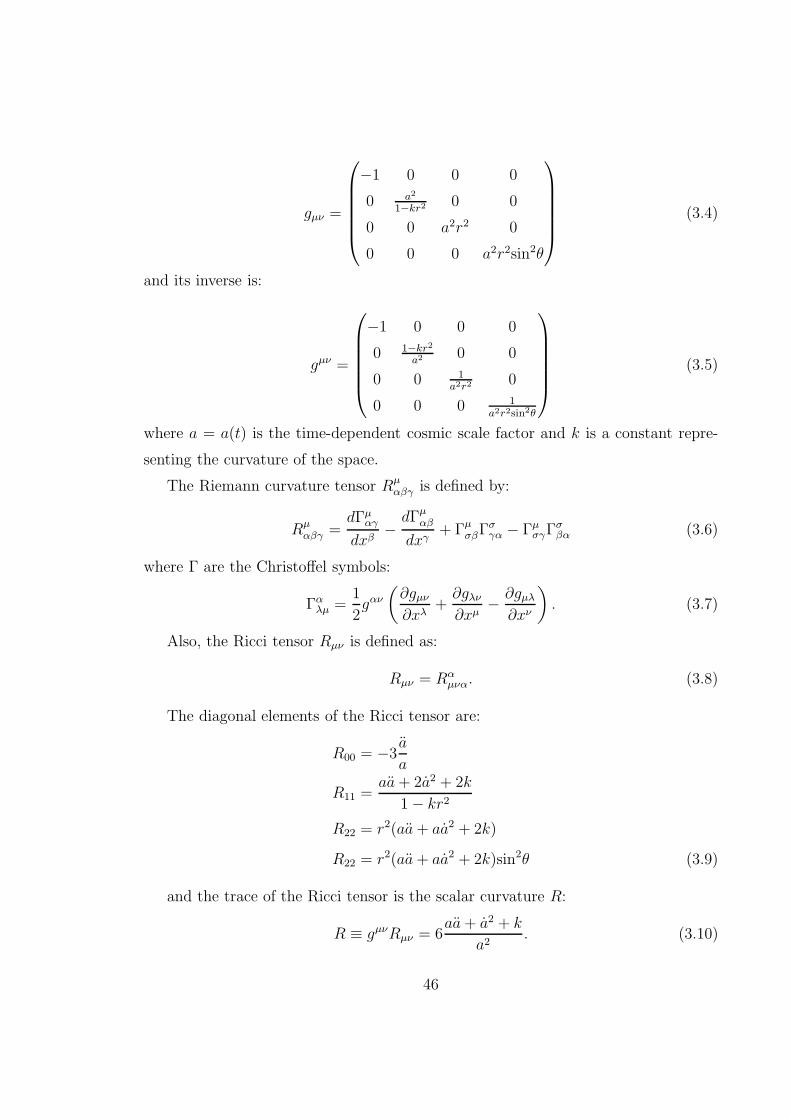
gµν =
−1 0 0 0
0 a2
1−kr20 0
0 0 a2r2 0
0 0 0 a2r2sin2θ
(3.4)
and its inverse is:
gµν =
−1 0 0 0
0 1−kr2
a20 0
0 0 1a2r2
0
0 0 0 1a2r2sin2θ
(3.5)
where a = a(t) is the time-dependent cosmic scale factor and k is a constant repre-
senting the curvature of the space.
The Riemann curvature tensor Rµαβγ is defined by:
Rµαβγ =
dΓµαγ
dxβ−dΓµ
αβ
dxγ+ Γµ
σβΓσγα − Γµ
σγΓσβα (3.6)
where Γ are the Christoffel symbols:
Γαλµ =
1
2gαν
(
∂gµν∂xλ
+∂gλν∂xµ
− ∂gµλ∂xν
)
. (3.7)
Also, the Ricci tensor Rµν is defined as:
Rµν = Rαµνα. (3.8)
The diagonal elements of the Ricci tensor are:
R00 = −3a
a
R11 =aa+ 2a2 + 2k
1− kr2
R22 = r2(aa+ aa2 + 2k)
R22 = r2(aa+ aa2 + 2k)sin2θ (3.9)
and the trace of the Ricci tensor is the scalar curvature R:
R ≡ gµνRµν = 6aa+ a2 + k
a2. (3.10)
46
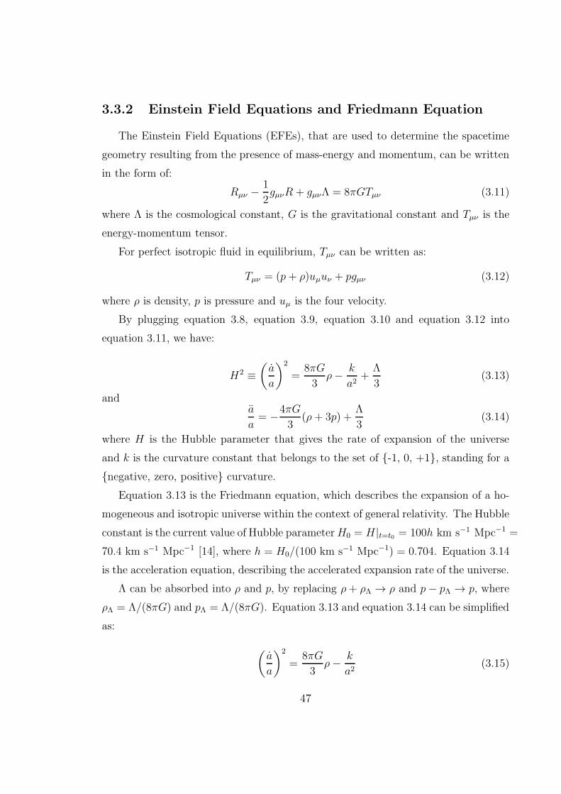
3.3.2 Einstein Field Equations and Friedmann Equation
The Einstein Field Equations (EFEs), that are used to determine the spacetime
geometry resulting from the presence of mass-energy and momentum, can be written
in the form of:
Rµν −1
2gµνR + gµνΛ = 8πGTµν (3.11)
where Λ is the cosmological constant, G is the gravitational constant and Tµν is the
energy-momentum tensor.
For perfect isotropic fluid in equilibrium, Tµν can be written as:
Tµν = (p+ ρ)uµuν + pgµν (3.12)
where ρ is density, p is pressure and uµ is the four velocity.
By plugging equation 3.8, equation 3.9, equation 3.10 and equation 3.12 into
equation 3.11, we have:
H2 ≡(
a
a
)2
=8πG
3ρ− k
a2+
Λ
3(3.13)
anda
a= −4πG
3(ρ+ 3p) +
Λ
3(3.14)
where H is the Hubble parameter that gives the rate of expansion of the universe
and k is the curvature constant that belongs to the set of -1, 0, +1, standing for a
negative, zero, positive curvature.
Equation 3.13 is the Friedmann equation, which describes the expansion of a ho-
mogeneous and isotropic universe within the context of general relativity. The Hubble
constant is the current value of Hubble parameterH0 = H|t=t0 = 100h km s−1 Mpc−1 =
70.4 km s−1 Mpc−1 [14], where h = H0/(100 km s−1 Mpc−1) = 0.704. Equation 3.14
is the acceleration equation, describing the accelerated expansion rate of the universe.
Λ can be absorbed into ρ and p, by replacing ρ+ ρΛ → ρ and p− pΛ → p, where
ρΛ = Λ/(8πG) and pΛ = Λ/(8πG). Equation 3.13 and equation 3.14 can be simplified
as:
(
a
a
)2
=8πG
3ρ− k
a2(3.15)
47
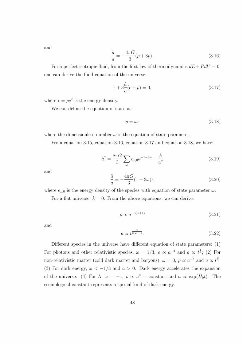
anda
a= −4πG
3(ρ+ 3p). (3.16)
For a perfect isotropic fluid, from the first law of thermodynamics dE+PdV = 0,
one can derive the fluid equation of the universe:
ǫ+ 3a
a(ǫ+ p) = 0, (3.17)
where ǫ = ρc2 is the energy density.
We can define the equation of state as:
p = ωǫ (3.18)
where the dimensionless number ω is the equation of state parameter.
From equation 3.15, equation 3.16, equation 3.17 and equation 3.18, we have:
a2 =8πG
3
∑
ω
ǫω,0a−1−3ω − k
a2(3.19)
anda
a= −4πG
3(1 + 3ω)ǫ. (3.20)
where ǫω,0 is the energy density of the species with equation of state parameter ω.
For a flat universe, k = 0. From the above equations, we can derive:
ρ ∝ a−3(ω+1) (3.21)
and
a ∝ t2
3(ω+1) . (3.22)
Different species in the universe have different equation of state parameters: (1)
For photons and other relativistic species, ω = 1/3, ρ ∝ a−4 and a ∝ t12 ; (2) For
non-relativistic matter (cold dark matter and baryons), ω = 0, ρ ∝ a−3 and a ∝ t23 ;
(3) For dark energy, ω < −1/3 and a > 0. Dark energy accelerates the expansion
of the universe. (4) For Λ, ω = −1, ρ ∝ a0 = constant and a ∝ exp(H0t). The
cosmological constant represents a special kind of dark energy.
48
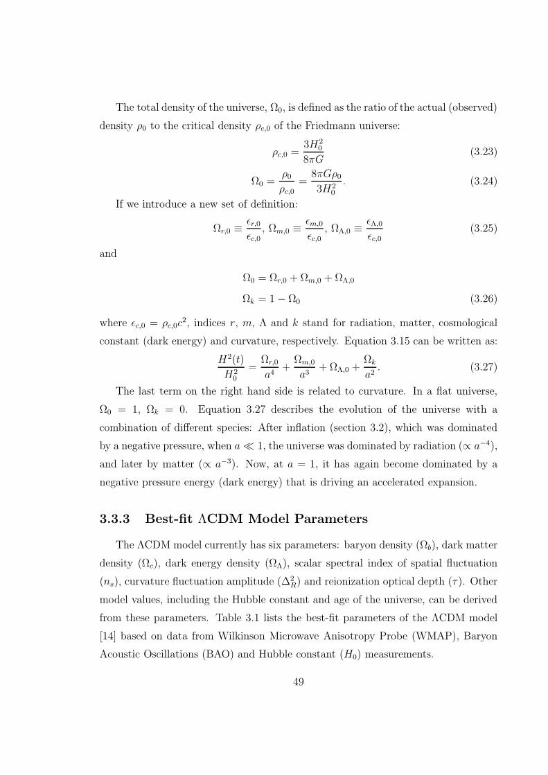
The total density of the universe, Ω0, is defined as the ratio of the actual (observed)
density ρ0 to the critical density ρc,0 of the Friedmann universe:
ρc,0 =3H2
0
8πG(3.23)
Ω0 =ρ0ρc,0
=8πGρ03H2
0
. (3.24)
If we introduce a new set of definition:
Ωr,0 ≡ǫr,0ǫc,0
, Ωm,0 ≡ǫm,0
ǫc,0, ΩΛ,0 ≡
ǫΛ,0ǫc,0
(3.25)
and
Ω0 = Ωr,0 + Ωm,0 + ΩΛ,0
Ωk = 1− Ω0 (3.26)
where ǫc,0 = ρc,0c2, indices r, m, Λ and k stand for radiation, matter, cosmological
constant (dark energy) and curvature, respectively. Equation 3.15 can be written as:
H2(t)
H20
=Ωr,0
a4+
Ωm,0
a3+ ΩΛ,0 +
Ωk
a2. (3.27)
The last term on the right hand side is related to curvature. In a flat universe,
Ω0 = 1, Ωk = 0. Equation 3.27 describes the evolution of the universe with a
combination of different species: After inflation (section 3.2), which was dominated
by a negative pressure, when a≪ 1, the universe was dominated by radiation (∝ a−4),
and later by matter (∝ a−3). Now, at a = 1, it has again become dominated by a
negative pressure energy (dark energy) that is driving an accelerated expansion.
3.3.3 Best-fit ΛCDM Model Parameters
The ΛCDM model currently has six parameters: baryon density (Ωb), dark matter
density (Ωc), dark energy density (ΩΛ), scalar spectral index of spatial fluctuation
(ns), curvature fluctuation amplitude (∆2R) and reionization optical depth (τ). Other
model values, including the Hubble constant and age of the universe, can be derived
from these parameters. Table 3.1 lists the best-fit parameters of the ΛCDM model
[14] based on data from Wilkinson Microwave Anisotropy Probe (WMAP), Baryon
Acoustic Oscillations (BAO) and Hubble constant (H0) measurements.
49
Table 3.1: Best-fit ΛCDM Model Parameters
Basic parameter Value DescriptionΩb 0.0456± 0.0016 Baryon densityΩc 0.227± 0.014 Cold dark matter densityΩΛ 0.728+0.015
−0.016 Dark energy densityns 0.963± 0.012 Scalar spectral index
∆2R(k0 = 0.002Mpc−1) (2.441+0.088
−0.092)× 10−9 Curvature fluctuation amplitudeτ 0.087± 0.014 Reionization optical depth
Extended parameter Value DescriptionH0 70.4+1.3
−1.4 Hubble constant (km s−1 Mpc−1)t0 13.75± 0.11 Age of the universe (Gyr)r < 0.24(95% CL) Tensor-to-scalar ratioΩ0 1.0023+0.0056
−0.0054 Total densityΩk −0.0023+0.0054
−0.0056 Curvature densityz∗ 1090.89+0.68
−0.69 Redshift at decouplingt∗ 377730+3205
−3200 Age at decoupling (yr)zreion 10.4± 1.2 Redshift of reionization
The universe is nearly flat
If the density of the universe, ρ0, is greater than critical density, ρc,0, then Ω0 > 1.0,
Ωk < 0, the geometry of space is closed. In this space, initially parallel photon paths
converge and return back to their starting point; If ρ0 < ρc,0, Ωk > 0, then the
geometry of space is open and negatively curved like the surface of a saddle; From
table 3.1, we have Ω0 = 1.0023+0.0056−0.0054, Ωk = −0.0023+0.0054
−0.0056. These measurements
show that the geometry of the universe is within measurement error of a flat space.
If flat or negatively curved, it is infinite in extent, unless the cosmological principle
does not hold on scales much greater than the horizon scale.
A solution to the flatness problem is given by the inflation theory (section 3.2).
It proposes a period of extremely rapid (a factor of ∼ 1026 in scale in only a small
fraction of a second) expansion of the universe prior to the more gradual Big Bang
expansion. Inflation stretches the geometry of the universe towards flatness.
50
Relativistic species in the universe
The main relativistic species are the Cosmic Microwave Background (CMB) pho-
tons (see section 3.4) and neutrinos. The energy density of photon can be calculated
by Bose-Einstein distribution:
ρ = g
∫
d3p
(2π)3f(~x, ~p)E(p), (3.28)
where, ρ is the energy density, g is the degeneracy, f(~x, ~p) is the distribution function,
and E(p) = (p2 +m2)1/2 is the energy at a given stage p.
For photons, g = 2, f(~x, ~p) = 1/(eE(p)/Tγ − 1) and E(p) = (p2 +m2)1/2 = p, thus
(note that d3p = 4πp2dp):
ργ = 2
∫
d3p
(2π)3p
ep/Tγ − 1
=8π
(2π)3
∫ ∞
0
p3
ep/Tγ − 1dp
=π2
15T 4γ (3.29)
So,
Ωγ,0 =ργ,0ρc,0
=π2
15T 4γ,0
1
ρc,0=π2
15T 4γ,0
8πG
3H20
=π2
15T 4γ,0h
−2 × 6.808× 10−7 = 4.98× 10⁻⁵ (3.30)
where Tγ,0 = 2.725 K is the temperature of the CMB measured today and h = 0.704.
Cosmic neutrinos have not been directly observed, because they are weakly inter-
acting particles. We can compute the relative energy density of neutrinos by relating
the temperature of neutrinos to the temperature of photons in CMB radiation, since
neutrinos were once in equilibrium with the rest of the cosmic plasma. Theory pre-
dicts Tν,0 ≈ 0.71 × Tγ,0 = 1.945 K and Ων,0 ≈ 0.68 × Ωγ,0 = 3.40 × 10⁻⁵. WMAP
has found that a cosmic neutrino background is also needed as a part of the standard
model of cosmology.
51
Matter in the universe
Observations have indicated the presence of dark matter in the universe, including
the rotation curves of galaxies, gravitational lensing of background objects by galaxy
clusters, the temperature distribution of hot gas in galaxies and clusters of galaxies,
and the CMB measurement, which can distinguish the dim baryon “dark matter”
from the non-baryonic dark matter.
There are three types of hypothetical dark matter: cold, warm and hot dark mat-
ter. Cold dark matter is the dark matter composed of particles with typical speeds
much below the speed of light (generally < 0.1c). Warm dark matter are particles
traveling at relativistic speeds, but less than ultra-relativistic speeds (typically be-
tween 0.1c and 0.95c). Hot dark matter are particles that travel at ultra-relativistic
velocities (> 0.95c). Cold dark matter is currently the area of greatest interest for
dark matter research, as hot and warm dark matter do not seem to be viable for
galaxy and galaxy cluster formation.
Most of the matter in the universe is cold dark matter. The measurements of
cosmic abundances of light elements suggest that the baryon density is only a small
fraction of the critical density. From table 3.1, we have Ωb = 0.0456 and Ωc = 0.227.
The cold dark matter constitute about 83% of the matter in the universe. The visible
universe (baryon) only contributes about 17% of the total mass and 4.56% of the
total mass-energy.
Weakly Interacting Massive Particles (WIMPs) are candidates for cold dark mat-
ter. These particles interact only through the weak force and gravity. WIMPs do
not interact via electromagnetism, so they cannot be observed directly. They do not
react with atomic nuclei because they do not interact with the strong force either.
There are many experiments currently running (or planned), aiming to search for
WIMPs [116, 117, 118, 119, 120]. WIMPs could also be produced in the laboratory.
Experiments with the Large Hadron Collider (LHC) may be able to detect WIMPs
produced in collisions of the proton beams.
Although WIMPs are a more popular dark matter candidate, there are also ex-
periments searching for other particle candidates. It is also possible that dark matter
52
consists of very heavy hidden sector particles that only interact with ordinary matter
via gravity.
Dark energy in the universe
Dark energy is a hypothetical energy that permeates the entire space and tends
to accelerate the expansion of the universe. Dark energy is the most accepted theory
to explain that the universe is expanding at an accelerating rate [121]. In the ΛCDM
model, dark energy needs to account for 72.8% of the total mass-energy of the universe
(table 3.1) to reconcile the measured flat geometry of space with the total density
equals the critical density. A direct signal of dark energy in a flat universe is from the
late-time Integrated Sachs-Wolfe effect (ISW) [122, 123, 124]. Dark energy is thought
to be homogeneous, and is not known to interact through any of the fundamental
forces other than gravity. With ω < −1/3, dark energy has negative pressure as
gravitational repulsion to accelerate the expension of the universe.
There are two proposed forms for dark energy: the cosmological constant and
scalar fields having a time-dependant energy density. The cosmological constant may
includes the contribution from scalar fields that are constant in time. It may be
difficult to distinguish scalar fields from the cosmological constant because the time
variation of the fields could be extremely small and the value of ω could be very close
to -1.
The simplest explanation for dark energy is the cosmological constant and the
simplest explanation for the cosmological constant is vacuum energy. That is, a
volume of space has some intrinsic, fundamental energy. There are many ways to
predict and estimate this energy, including quantum field theory and string theory.
The cosmological constant remains a subject of theoretical and empirical interest.
The explanation of this small but positive value is still an outstanding challenge.
53
3.4 The Cosmic Microwave Background Radiation
Figure 3.1 shows the timelime of CMB radiation formation. The ΛCDM model
includes the abrupt appearance of expanding space-time containing radiation at tem-
peratures of around 1019 K. The universe was intensely hot, remarkably smooth and
essentially homogeneous. However, small fluctuations in density originating as quan-
tum fluctuations, began to appear and grow. Inflation stretched the curvature of the
universe to be nearly (but not exactly) flat and expanded these quantum fluctuations
in the density of the early universe to the cosmic scale. At redshift (z > 1100), when
the temperature was still above 3000 K, photons were tightly coupled to free electrons
through Thomson scattering. As the universe cooled down to about 3000 K, clumps
of matter (baryons) began to condense and within them protons captured electrons
and became atoms (recombination). Radiation decoupled from matter at 377730+3205−3200
years (table 3.1) after the Big Bang. The last scattering of the CMB photons was at
redshift of about 1100, at which point the universe was almost exclusively composed
of hydrogen, helium, dark matter, photons and neutrinos. This is the period when the
CMB radiation was last scattered. After that, the CMB photons were free streaming.
The color temperature of the CMB photons has continued to diminish ever since
the Last Scattering Surface (LSS) and now down to about 2.7 K. Their tempera-
ture will continue dropping as the universe expands. The radiation from the sky we
measure today comes from the surface of last scattering (figure 3.1). Most of the
radiation energy in the universe is in the CMB radiation, making up a fraction of
roughly 5× 10⁻⁵ (equation 3.30) of the total density of the universe.
Precise measurements of cosmic background radiation are critical to cosmology.
The CMB has a thermal black body spectrum at a temperature of 2.725 K. In the
Planck spectrum, it peaks at the microwave range frequency of about 160.2 GHz,
corresponding to a 1.873 mm wavelength (see appendix B for details).
54
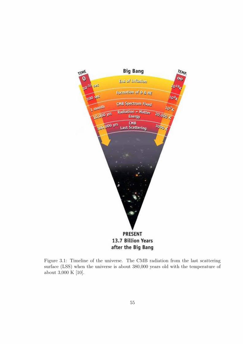
Figure 3.1: Timeline of the universe. The CMB radiation from the last scatteringsurface (LSS) when the universe is about 380,000 years old with the temperature ofabout 3,000 K [10].
55
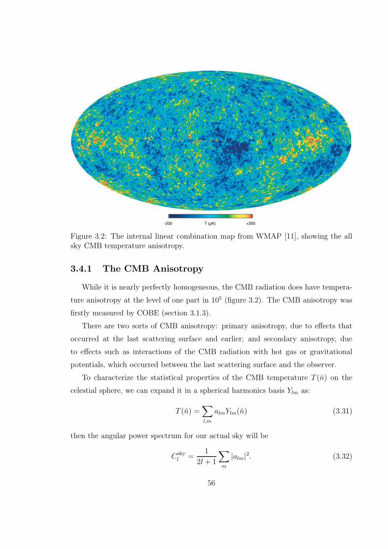
Figure 3.2: The internal linear combination map from WMAP [11], showing the allsky CMB temperature anisotropy.
3.4.1 The CMB Anisotropy
While it is nearly perfectly homogeneous, the CMB radiation does have tempera-
ture anisotropy at the level of one part in 105 (figure 3.2). The CMB anisotropy was
firstly measured by COBE (section 3.1.3).
There are two sorts of CMB anisotropy: primary anisotropy, due to effects that
occurred at the last scattering surface and earlier; and secondary anisotropy, due
to effects such as interactions of the CMB radiation with hot gas or gravitational
potentials, which occurred between the last scattering surface and the observer.
To characterize the statistical properties of the CMB temperature T (n) on the
celestial sphere, we can expand it in a spherical harmonics basis Ylm as:
T (n) =∑
l,m
almYlm(n) (3.31)
then the angular power spectrum for our actual sky will be
Cskyl =
1
2l + 1
∑
m
|alm|2. (3.32)
56
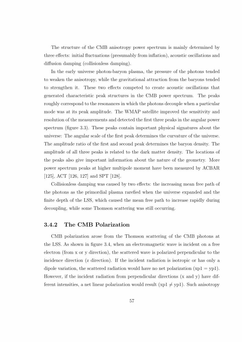
The structure of the CMB anisotropy power spectrum is mainly determined by
three effects: initial fluctuations (presumably from inflation), acoustic oscillations and
diffusion damping (collisionless damping).
In the early universe photon-baryon plasma, the pressure of the photons tended
to weaken the anisotropy, while the gravitational attraction from the baryons tended
to strengthen it. These two effects competed to create acoustic oscillations that
generated characteristic peak structures in the CMB power spectrum. The peaks
roughly correspond to the resonances in which the photons decouple when a particular
mode was at its peak amplitude. The WMAP satellite improved the sensitivity and
resolution of the measurements and detected the first three peaks in the angular power
spectrum (figure 3.3). These peaks contain important physical signatures about the
universe: The angular scale of the first peak determines the curvature of the universe.
The amplitude ratio of the first and second peak determines the baryon density. The
amplitude of all three peaks is related to the dark matter density. The locations of
the peaks also give important information about the nature of the geometry. More
power spectrum peaks at higher multipole moment have been measured by ACBAR
[125], ACT [126, 127] and SPT [128].
Collisionless damping was caused by two effects: the increasing mean free path of
the photons as the primordial plasma rarefied when the universe expanded and the
finite depth of the LSS, which caused the mean free path to increase rapidly during
decoupling, while some Thomson scattering was still occurring.
3.4.2 The CMB Polarization
CMB polarization arose from the Thomson scattering of the CMB photons at
the LSS. As shown in figure 3.4, when an electromagnetic wave is incident on a free
electron (from x or y direction), the scattered wave is polarized perpendicular to the
incidence direction (z direction). If the incident radiation is isotropic or has only a
dipole variation, the scattered radiation would have no net polarization (xp1 = yp1).
However, if the incident radiation from perpendicular directions (x and y) have dif-
ferent intensities, a net linear polarization would result (xp1 6= yp1). Such anisotropy
57
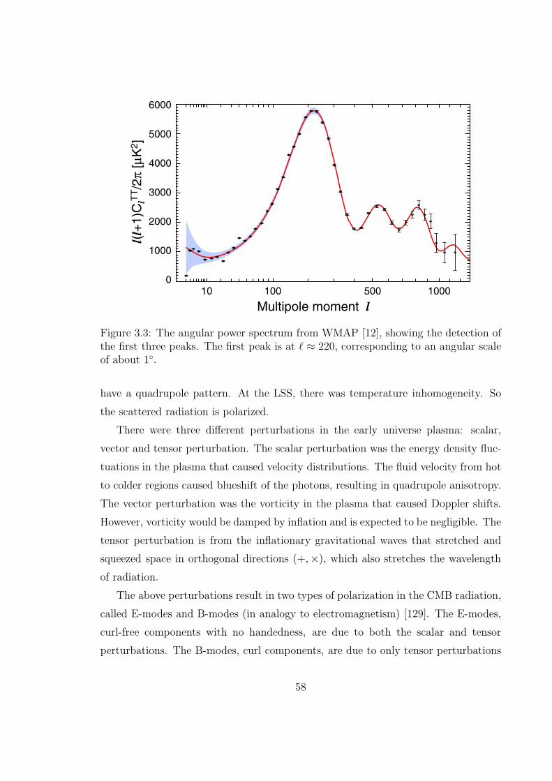
Figure 3.3: The angular power spectrum from WMAP [12], showing the detection ofthe first three peaks. The first peak is at ℓ ≈ 220, corresponding to an angular scaleof about 1.
have a quadrupole pattern. At the LSS, there was temperature inhomogeneity. So
the scattered radiation is polarized.
There were three different perturbations in the early universe plasma: scalar,
vector and tensor perturbation. The scalar perturbation was the energy density fluc-
tuations in the plasma that caused velocity distributions. The fluid velocity from hot
to colder regions caused blueshift of the photons, resulting in quadrupole anisotropy.
The vector perturbation was the vorticity in the plasma that caused Doppler shifts.
However, vorticity would be damped by inflation and is expected to be negligible. The
tensor perturbation is from the inflationary gravitational waves that stretched and
squeezed space in orthogonal directions (+,×), which also stretches the wavelength
of radiation.
The above perturbations result in two types of polarization in the CMB radiation,
called E-modes and B-modes (in analogy to electromagnetism) [129]. The E-modes,
curl-free components with no handedness, are due to both the scalar and tensor
perturbations. The B-modes, curl components, are due to only tensor perturbations
58
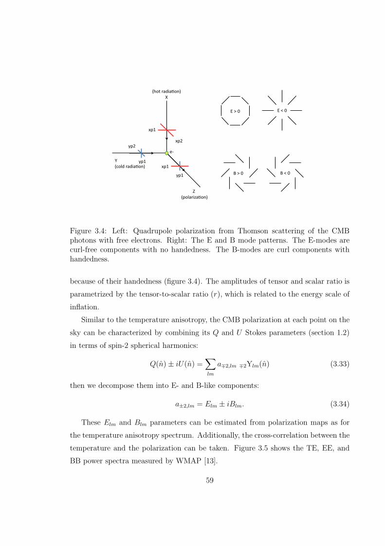
(hot radiaon)
X
Y
(cold radiaon)
Z
(polarizaon)
xp1
xp2 yp2
yp1
yp1
xp1
e-
E > 0 E < 0
B > 0 B < 0
Figure 3.4: Left: Quadrupole polarization from Thomson scattering of the CMBphotons with free electrons. Right: The E and B mode patterns. The E-modes arecurl-free components with no handedness. The B-modes are curl components withhandedness.
because of their handedness (figure 3.4). The amplitudes of tensor and scalar ratio is
parametrized by the tensor-to-scalar ratio (r), which is related to the energy scale of
inflation.
Similar to the temperature anisotropy, the CMB polarization at each point on the
sky can be characterized by combining its Q and U Stokes parameters (section 1.2)
in terms of spin-2 spherical harmonics:
Q(n)± iU(n) =∑
lm
a∓2,lm ∓2Ylm(n) (3.33)
then we decompose them into E- and B-like components:
a±2,lm = Elm ± iBlm. (3.34)
These Elm and Blm parameters can be estimated from polarization maps as for
the temperature anisotropy spectrum. Additionally, the cross-correlation between the
temperature and the polarization can be taken. Figure 3.5 shows the TE, EE, and
BB power spectra measured by WMAP [13].
59
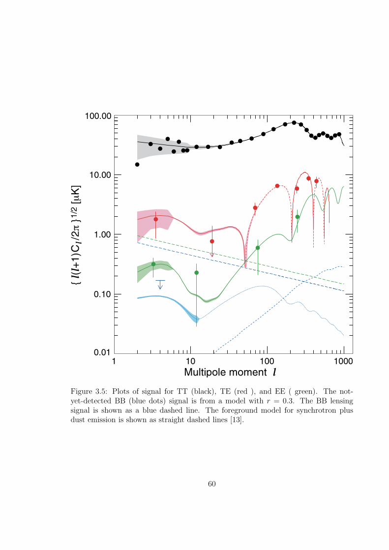
Figure 3.5: Plots of signal for TT (black), TE (red ), and EE ( green). The not-yet-detected BB (blue dots) signal is from a model with r = 0.3. The BB lensingsignal is shown as a blue dashed line. The foreground model for synchrotron plusdust emission is shown as straight dashed lines [13].
60
The E-modes polarization had been measured over a range of angular scales [130,
131]. The B-modes, which have not been detected, are expected to be extraordinarily
faint. To set meaningful limits on inflationary models, any experiment designed to
detect the inflationary B-mode signal should have a polarization sensitivity near 30
nK. That is 10−8 of the CMB blackbody temperature and 10−3 of the primordial
CMB temperature anisotropy. The B-mode observation provides the only known way
to measure the energy scale of inflation since inflation produced these gravitational
waves whose amplitude depends only on the energy scale at which inflation occurred.
Detection of B-modes would also be the first ever direct detection of gravitational
waves.
61
Chapter 4
The Cosmology Large Angular
Scale Surveyor (CLASS)
In chapter 3, we discussed the origin and evolution of the universe. A fundamental
question is, “Did inflation really happen?” Inflation posits that the universe grew from
quantum fluctuations of the vacuum driven by negative pressure energy to expand
exponentially to astronomical scales. The simplest (and therefore most compelling)
versions of inflation produce a stochastic background of gravitational waves whose
amplitude depends only on the energy scale at which inflation occurred. The gravita-
tional waves imprint a polarization pattern on the CMB (B-mode polarization), that
then provides a direct way to measure the energy scale of inflation (section 3.4.2).
Measurements to date of the E-mode signal are consistent with the predictions
of anisotropic Thompson scattering [130, 131], while the B-mode signal has yet to
be detected. The B-mode power spectrum amplitude can be parameterized by the
relative amplitude of the tensor to scalar modes (the tensor-to-scalar ratio), given by
r ≡ ∆2h(k0)
∆2ℜ(k0)
, (4.1)
where, ∆2ℜ(k) and ∆2
h(k) denote the dimensionless scalar and tensor power spectra, ℜdenotes the intrinsic curvature perturbation, h denotes the amplitude of gravitational
waves, and k0 is some pivot wavenumber [132, 133].
62
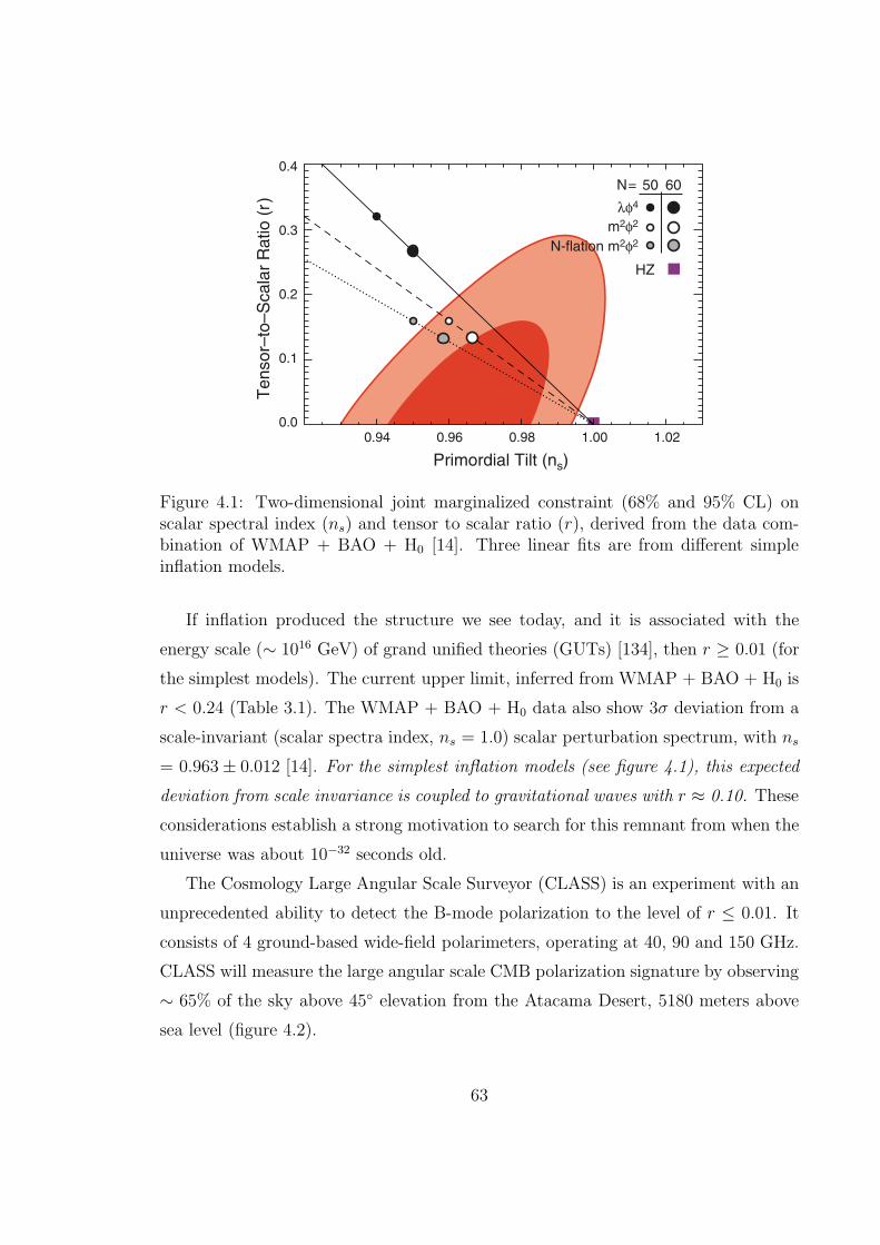
Figure 4.1: Two-dimensional joint marginalized constraint (68% and 95% CL) onscalar spectral index (ns) and tensor to scalar ratio (r), derived from the data com-bination of WMAP + BAO + H0 [14]. Three linear fits are from different simpleinflation models.
If inflation produced the structure we see today, and it is associated with the
energy scale (∼ 1016 GeV) of grand unified theories (GUTs) [134], then r ≥ 0.01 (for
the simplest models). The current upper limit, inferred from WMAP + BAO + H0 is
r < 0.24 (Table 3.1). The WMAP + BAO + H0 data also show 3σ deviation from a
scale-invariant (scalar spectra index, ns = 1.0) scalar perturbation spectrum, with ns
= 0.963± 0.012 [14]. For the simplest inflation models (see figure 4.1), this expected
deviation from scale invariance is coupled to gravitational waves with r ≈ 0.10. These
considerations establish a strong motivation to search for this remnant from when the
universe was about 10−32 seconds old.
The Cosmology Large Angular Scale Surveyor (CLASS) is an experiment with an
unprecedented ability to detect the B-mode polarization to the level of r ≤ 0.01. It
consists of 4 ground-based wide-field polarimeters, operating at 40, 90 and 150 GHz.
CLASS will measure the large angular scale CMB polarization signature by observing
∼ 65% of the sky above 45 elevation from the Atacama Desert, 5180 meters above
sea level (figure 4.2).
63
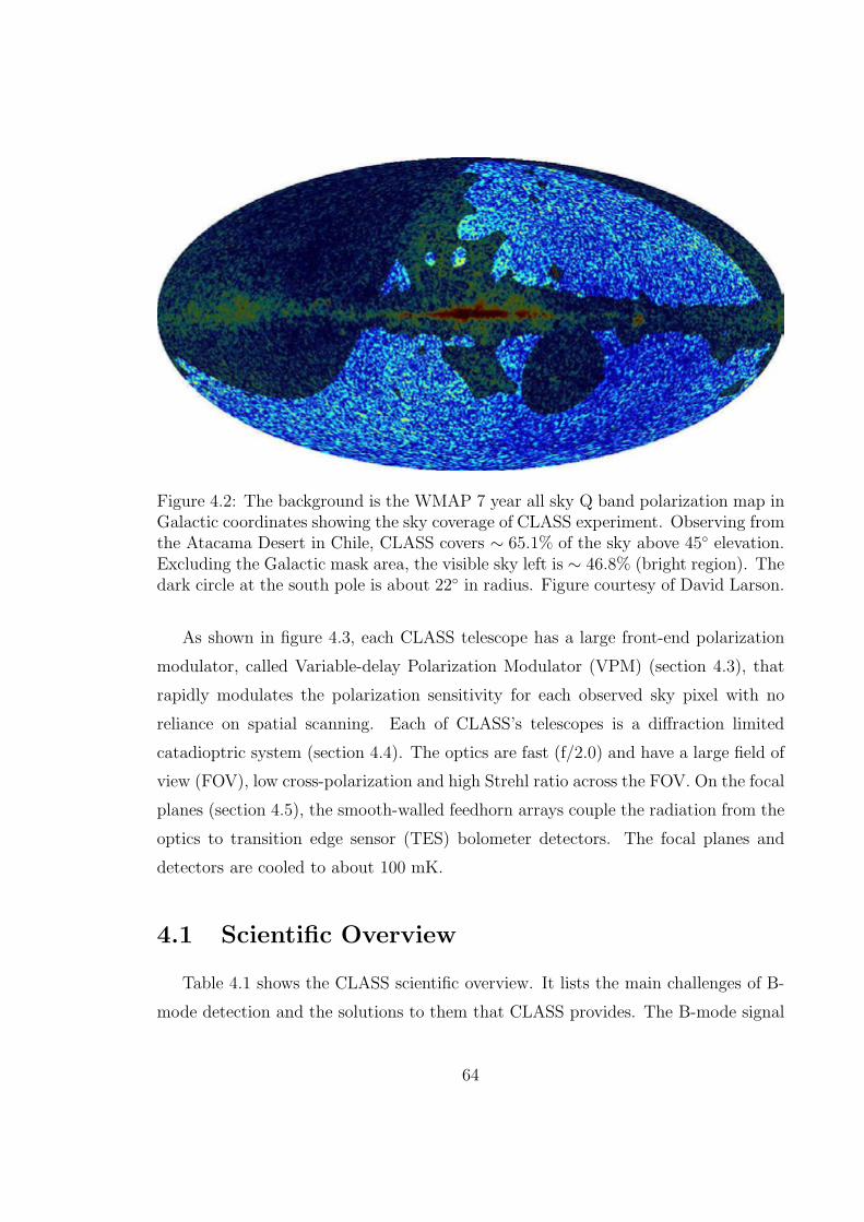
Figure 4.2: The background is the WMAP 7 year all sky Q band polarization map inGalactic coordinates showing the sky coverage of CLASS experiment. Observing fromthe Atacama Desert in Chile, CLASS covers ∼ 65.1% of the sky above 45 elevation.Excluding the Galactic mask area, the visible sky left is ∼ 46.8% (bright region). Thedark circle at the south pole is about 22 in radius. Figure courtesy of David Larson.
As shown in figure 4.3, each CLASS telescope has a large front-end polarization
modulator, called Variable-delay Polarization Modulator (VPM) (section 4.3), that
rapidly modulates the polarization sensitivity for each observed sky pixel with no
reliance on spatial scanning. Each of CLASS’s telescopes is a diffraction limited
catadioptric system (section 4.4). The optics are fast (f/2.0) and have a large field of
view (FOV), low cross-polarization and high Strehl ratio across the FOV. On the focal
planes (section 4.5), the smooth-walled feedhorn arrays couple the radiation from the
optics to transition edge sensor (TES) bolometer detectors. The focal planes and
detectors are cooled to about 100 mK.
4.1 Scientific Overview
Table 4.1 shows the CLASS scientific overview. It lists the main challenges of B-
mode detection and the solutions to them that CLASS provides. The B-mode signal
64
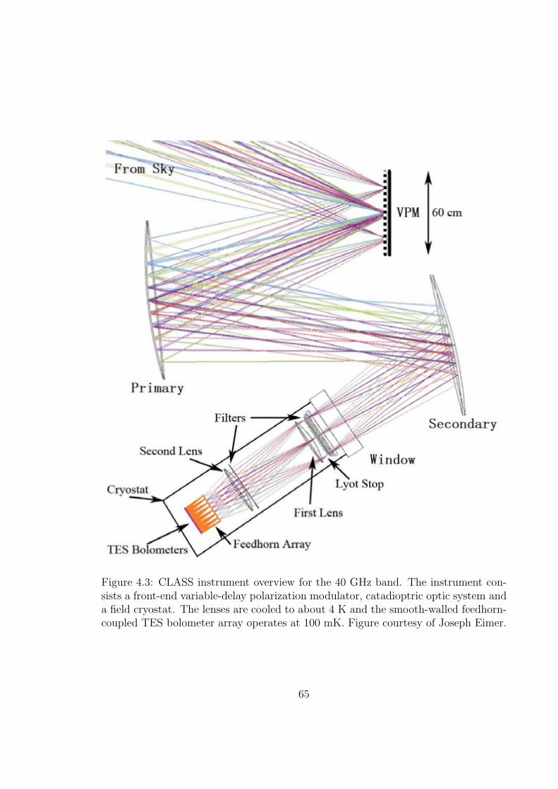
Figure 4.3: CLASS instrument overview for the 40 GHz band. The instrument con-sists a front-end variable-delay polarization modulator, catadioptric optic system anda field cryostat. The lenses are cooled to about 4 K and the smooth-walled feedhorn-coupled TES bolometer array operates at 100 mK. Figure courtesy of Joseph Eimer.
65
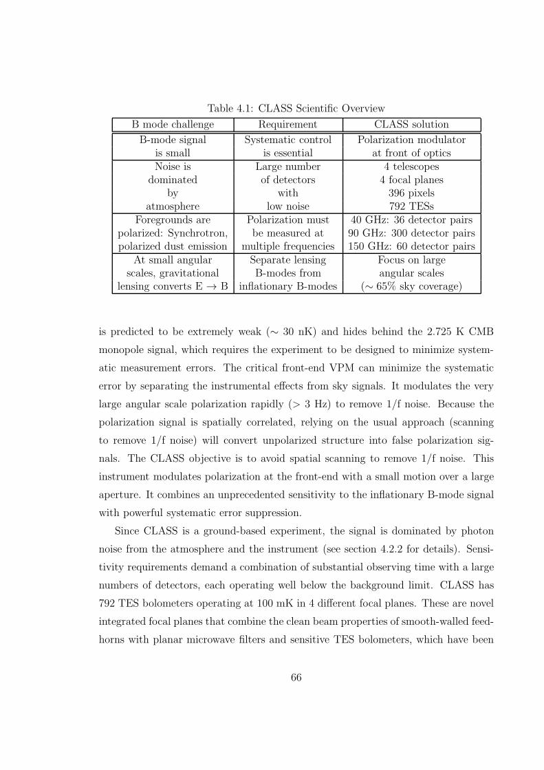
Table 4.1: CLASS Scientific Overview
B mode challenge Requirement CLASS solution
B-mode signal Systematic control Polarization modulatoris small is essential at front of opticsNoise is Large number 4 telescopes
dominated of detectors 4 focal planesby with 396 pixels
atmosphere low noise 792 TESsForegrounds are Polarization must 40 GHz: 36 detector pairs
polarized: Synchrotron, be measured at 90 GHz: 300 detector pairspolarized dust emission multiple frequencies 150 GHz: 60 detector pairs
At small angular Separate lensing Focus on largescales, gravitational B-modes from angular scales
lensing converts E → B inflationary B-modes (∼ 65% sky coverage)
is predicted to be extremely weak (∼ 30 nK) and hides behind the 2.725 K CMB
monopole signal, which requires the experiment to be designed to minimize system-
atic measurement errors. The critical front-end VPM can minimize the systematic
error by separating the instrumental effects from sky signals. It modulates the very
large angular scale polarization rapidly (> 3 Hz) to remove 1/f noise. Because the
polarization signal is spatially correlated, relying on the usual approach (scanning
to remove 1/f noise) will convert unpolarized structure into false polarization sig-
nals. The CLASS objective is to avoid spatial scanning to remove 1/f noise. This
instrument modulates polarization at the front-end with a small motion over a large
aperture. It combines an unprecedented sensitivity to the inflationary B-mode signal
with powerful systematic error suppression.
Since CLASS is a ground-based experiment, the signal is dominated by photon
noise from the atmosphere and the instrument (see section 4.2.2 for details). Sensi-
tivity requirements demand a combination of substantial observing time with a large
numbers of detectors, each operating well below the background limit. CLASS has
792 TES bolometers operating at 100 mK in 4 different focal planes. These are novel
integrated focal planes that combine the clean beam properties of smooth-walled feed-
horns with planar microwave filters and sensitive TES bolometers, which have been
66
demonstrated in astronomical instruments [135].
To characterize the Galactic foreground contamination from synchrotron and po-
larized dust emission (section 1.4), CLASS observes in three frequency bands (40,
90 and 150 GHz), accessible from the ground, as seen in figure 4.4. The data from
these bands will be used to characterize the foreground signals for subsequent re-
moval. Free-free emission is unpolarized so it does not affect the CMB polarization
measurement.
Gravitational lensing can convert E-mode polarization to B-mode polarization in
small angular scales, but on large angular scales inflation is the only known extra-
galactic source of B-mode polarization. Thus, observations of the large angular scale
CMB polarization signals provide a clean way to directly verify inflation and measure
the energy scale of inflation [136]. By targeting the large scale “reionization bump” of
the B-mode signal at l ≤ 10, where the B-mode signal emerges most clearly from the
gravitational lensing foreground, CLASS avoids gravitational lensing contamination
(see section 4.2).
In summary, the CLASS experiment has the following design criteria for B-mode
searching: (1) Improves instrument sensitivity by using a larger number of back-
ground limited detectors; (2) Achieves excellent systematic control by placing the
polarization modulator at front of the optics; (3) Observes in multi-waveband for
foreground removal. (4) Focuses on large angular scale to avoid gravitational lensing
contamination.
4.2 Sensitivity Calculation and Bandpass Optimiza-
tion
Figure 4.4 shows the results of CLASS waveband optimization and sensitivity
calculation. CLASS observing near the frequency of minimum Galactic foregrounds,
achieves maximum sensitivity to the level of r ∼ 0.01 at the “reionization bump”
and avoids the lensing contamination that dominates at small scales. Additional
experiments, such as PIPER [137], SPIDER [138], and EBEX [139] will take various
67
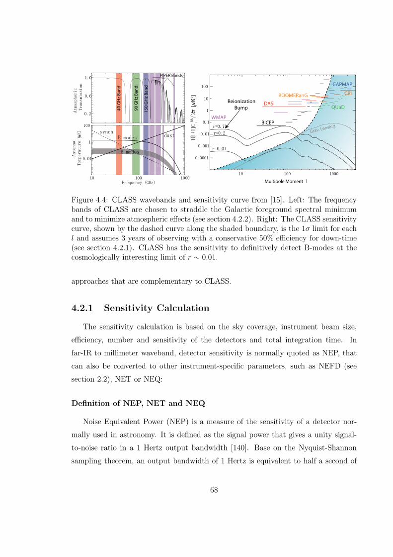
µ
dn
aB z
HG
04
dn
aB z
HG
09
dn
aB z
HG
05
1
PIPER Bands
Multipole Moment
)π
[µK
2]
Grav. Lensing
Reionization
Bump
BOOMERanG
DASI
WMAP
QUaD
CBI
CAPMAP
BICEP
Figure 4.4: CLASS wavebands and sensitivity curve from [15]. Left: The frequencybands of CLASS are chosen to straddle the Galactic foreground spectral minimumand to minimize atmospheric effects (see section 4.2.2). Right: The CLASS sensitivitycurve, shown by the dashed curve along the shaded boundary, is the 1σ limit for eachl and assumes 3 years of observing with a conservative 50% efficiency for down-time(see section 4.2.1). CLASS has the sensitivity to definitively detect B-modes at thecosmologically interesting limit of r ∼ 0.01.
approaches that are complementary to CLASS.
4.2.1 Sensitivity Calculation
The sensitivity calculation is based on the sky coverage, instrument beam size,
efficiency, number and sensitivity of the detectors and total integration time. In
far-IR to millimeter waveband, detector sensitivity is normally quoted as NEP, that
can also be converted to other instrument-specific parameters, such as NEFD (see
section 2.2), NET or NEQ:
Definition of NEP, NET and NEQ
Noise Equivalent Power (NEP) is a measure of the sensitivity of a detector nor-
mally used in astronomy. It is defined as the signal power that gives a unity signal-
to-noise ratio in a 1 Hertz output bandwidth [140]. Base on the Nyquist-Shannon
sampling theorem, an output bandwidth of 1 Hertz is equivalent to half a second of
68
integration time. NEP is a detector-specific parameter. It has the unit of WHz−1/2.
NET is Noise Equivalent Temperature. It is defined as the signal (in temperature
units) from a source needed to produce a signal-to-noise ratio value of unity in a 1.0
second integration [141]. It is an instrument-specific parameter and quoted in units
of µKs1/2.
To measure polarization signal, we have an equivalent definition to the NET, that
is Noise Equivalent Q Stokes parameter (NEQ). It is defined as the polarized signal
from a linearly polarized source aligned with the detector orientation that is required
to produce a signal-to-noise ratio value of unity in a 1.0 second integration. It is also
quoted in units of µKs1/2.
The above definitions can be quoted for a single detector or a pair of detectors
following the relations:
NEPs =√2NEPp
NETs =√2NETp
NEQs =√2NEQp (4.2)
where the indices “s” means a single detector and “p” means a detector pair.
The conversion between NET and NEP is [142]:
NET =NEP√
2ηdηtAΩ∆ν∂Bν/∂T(4.3)
where, ηd and ηt are the detector and instrument efficiencies, AΩ describes the optics,
∆ν is the bandwidth and ∂Bν/∂T is the derivative of the source emission (the CMB)
with respect to temperature (Tcmb). The factor of√2 is from the conversion between
Hz and second. We also have [141]:
NEQs =√2NEQp = 2NETs = 2
√2NETp (4.4)
Table 4.2 shows CLASS detector sensitivities in NEQp.
69
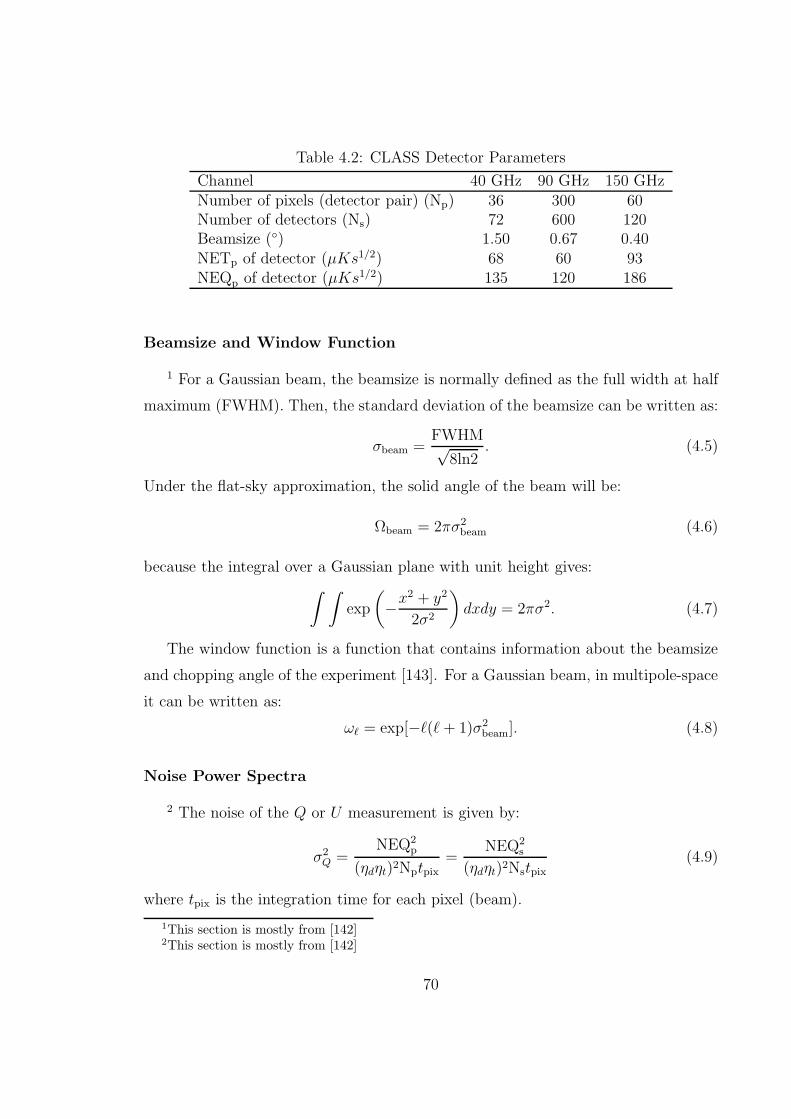
Table 4.2: CLASS Detector Parameters
Channel 40 GHz 90 GHz 150 GHzNumber of pixels (detector pair) (Np) 36 300 60Number of detectors (Ns) 72 600 120Beamsize () 1.50 0.67 0.40NETp of detector (µKs1/2) 68 60 93NEQp of detector (µKs1/2) 135 120 186
Beamsize and Window Function
1 For a Gaussian beam, the beamsize is normally defined as the full width at half
maximum (FWHM). Then, the standard deviation of the beamsize can be written as:
σbeam =FWHM√
8ln2. (4.5)
Under the flat-sky approximation, the solid angle of the beam will be:
Ωbeam = 2πσ2beam (4.6)
because the integral over a Gaussian plane with unit height gives:
∫ ∫
exp
(
−x2 + y2
2σ2
)
dxdy = 2πσ2. (4.7)
The window function is a function that contains information about the beamsize
and chopping angle of the experiment [143]. For a Gaussian beam, in multipole-space
it can be written as:
ωℓ = exp[−ℓ(ℓ + 1)σ2beam]. (4.8)
Noise Power Spectra
2 The noise of the Q or U measurement is given by:
σ2Q =
NEQ2p
(ηdηt)2Nptpix=
NEQ2s
(ηdηt)2Nstpix(4.9)
where tpix is the integration time for each pixel (beam).
1This section is mostly from [142]2This section is mostly from [142]
70
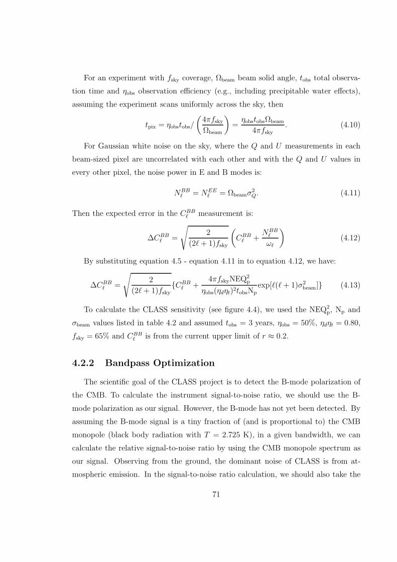
For an experiment with fsky coverage, Ωbeam beam solid angle, tobs total observa-
tion time and ηobs observation efficiency (e.g., including precipitable water effects),
assuming the experiment scans uniformly across the sky, then
tpix = ηobstobs/
(
4πfskyΩbeam
)
=ηobstobsΩbeam
4πfsky. (4.10)
For Gaussian white noise on the sky, where the Q and U measurements in each
beam-sized pixel are uncorrelated with each other and with the Q and U values in
every other pixel, the noise power in E and B modes is:
NBBℓ = NEE
ℓ = Ωbeamσ2Q. (4.11)
Then the expected error in the CBBℓ measurement is:
∆CBBℓ =
√
2
(2ℓ+ 1)fsky
(
CBBℓ +
NBBℓ
ωℓ
)
(4.12)
By substituting equation 4.5 - equation 4.11 in to equation 4.12, we have:
∆CBBℓ =
√
2
(2ℓ+ 1)fskyCBB
ℓ +4πfskyNEQ
2p
ηobs(ηdηt)2tobsNp
exp[ℓ(ℓ+ 1)σ2beam] (4.13)
To calculate the CLASS sensitivity (see figure 4.4), we used the NEQ2p, Np and
σbeam values listed in table 4.2 and assumed tobs = 3 years, ηobs = 50%, ηdηt = 0.80,
fsky = 65% and CBBℓ is from the current upper limit of r ≈ 0.2.
4.2.2 Bandpass Optimization
The scientific goal of the CLASS project is to detect the B-mode polarization of
the CMB. To calculate the instrument signal-to-noise ratio, we should use the B-
mode polarization as our signal. However, the B-mode has not yet been detected. By
assuming the B-mode signal is a tiny fraction of (and is proportional to) the CMB
monopole (black body radiation with T = 2.725 K), in a given bandwidth, we can
calculate the relative signal-to-noise ratio by using the CMB monopole spectrum as
our signal. Observing from the ground, the dominant noise of CLASS is from at-
mospheric emission. In the signal-to-noise ratio calculation, we should also take the
71
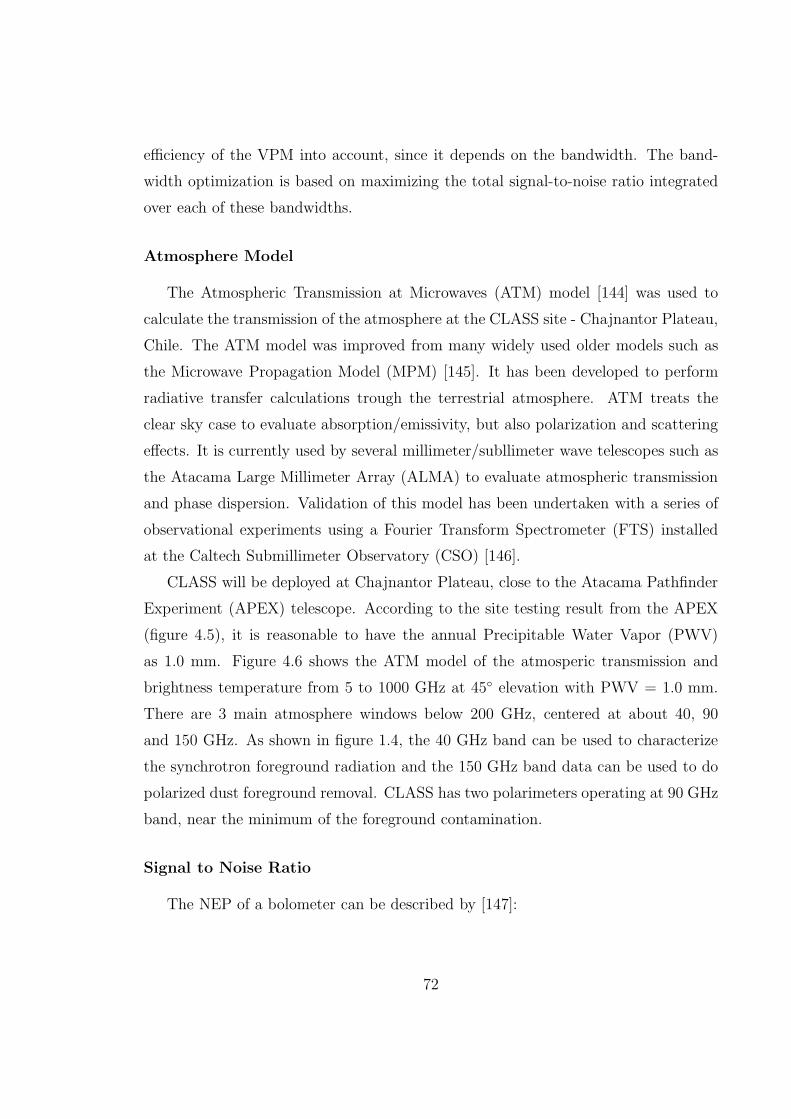
efficiency of the VPM into account, since it depends on the bandwidth. The band-
width optimization is based on maximizing the total signal-to-noise ratio integrated
over each of these bandwidths.
Atmosphere Model
The Atmospheric Transmission at Microwaves (ATM) model [144] was used to
calculate the transmission of the atmosphere at the CLASS site - Chajnantor Plateau,
Chile. The ATM model was improved from many widely used older models such as
the Microwave Propagation Model (MPM) [145]. It has been developed to perform
radiative transfer calculations trough the terrestrial atmosphere. ATM treats the
clear sky case to evaluate absorption/emissivity, but also polarization and scattering
effects. It is currently used by several millimeter/subllimeter wave telescopes such as
the Atacama Large Millimeter Array (ALMA) to evaluate atmospheric transmission
and phase dispersion. Validation of this model has been undertaken with a series of
observational experiments using a Fourier Transform Spectrometer (FTS) installed
at the Caltech Submillimeter Observatory (CSO) [146].
CLASS will be deployed at Chajnantor Plateau, close to the Atacama Pathfinder
Experiment (APEX) telescope. According to the site testing result from the APEX
(figure 4.5), it is reasonable to have the annual Precipitable Water Vapor (PWV)
as 1.0 mm. Figure 4.6 shows the ATM model of the atmosperic transmission and
brightness temperature from 5 to 1000 GHz at 45 elevation with PWV = 1.0 mm.
There are 3 main atmosphere windows below 200 GHz, centered at about 40, 90
and 150 GHz. As shown in figure 1.4, the 40 GHz band can be used to characterize
the synchrotron foreground radiation and the 150 GHz band data can be used to do
polarized dust foreground removal. CLASS has two polarimeters operating at 90 GHz
band, near the minimum of the foreground contamination.
Signal to Noise Ratio
The NEP of a bolometer can be described by [147]:
72
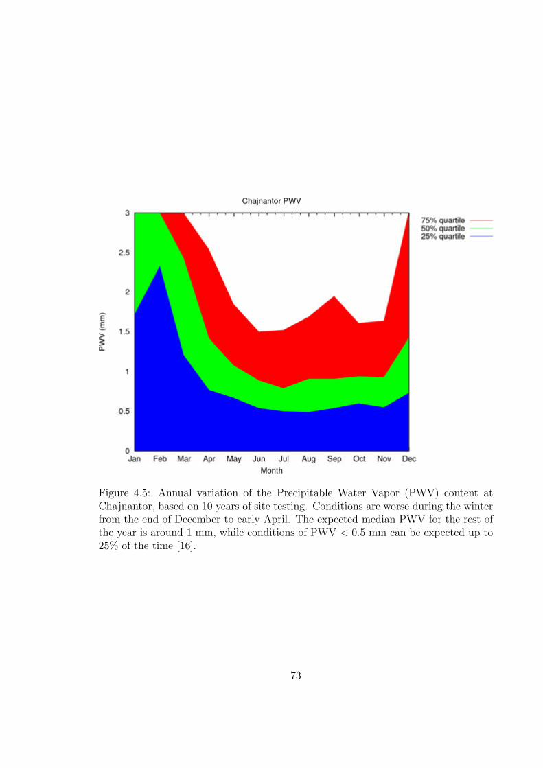
Figure 4.5: Annual variation of the Precipitable Water Vapor (PWV) content atChajnantor, based on 10 years of site testing. Conditions are worse during the winterfrom the end of December to early April. The expected median PWV for the rest ofthe year is around 1 mm, while conditions of PWV < 0.5 mm can be expected up to25% of the time [16].
73
0 100 200 300 400 500 600 700 800 900 10000
0.1
0.2
0.3
0.4
0.5
0.6
0.7
0.8
0.9
1Atmospheric Transmission
Frequency (GHz)
Tran
smis
sion
0 100 200 300 400 500 600 700 800 900 10000
50
100
150
200
250
300Atmospheric Brightness Temperature
Frequency (GHz)
Brig
htne
ss T
empe
ratu
re (K
)
Figure 4.6: Atmospheric transmission and brightness temperature at CLASS site from5 to 1000 GHz. ATM parameters: ground temperature = 275 K, ground pressure= 558 mb, PWV = 1.0 mm, elevation = 45, altidude = 5180 m. ATM version:atm2011 03 15.exe.
NEP2 = NEP2Johnson +NEP2
thermal +NEP2photon
+NEP2load +NEP2
amplifier +NEP2excess. (4.14)
Since detectors for the CLASS experiment are background limited, NEP2photon from
atmosphere and instrument dominates over other sources of noise. In a black-body
radiation field, NEP2photon can be written as [147] (see appendix C for details):
NEP2photon = 4
AΩ
c2(kBTs)
5
h3
∫
x4
ex − 1
(
1 +αǫf
ex − 1
)
(αǫf)dx (4.15)
Where AΩ describes the optics, f is the transmissivity of the optics, Ts is the tem-
perature of the source, ǫ is the emissivity of the source, α is the detector absorptivity,
α, ǫ, and f are evaluated at ν, and x = hν/(kBTs).
The atmosphere is treated as a blackbody source with varying emissivity:
Iν =
(
2hν3/c2
ehν/(kBTs) − 1
)
ǫ (4.16)
where Iν is the intensity of the atmosphere emission.
74
The number of photons in a given state x is:
n(ν) = n(x) =αǫf
ex − 1. (4.17)
From equation 4.16 and equation 4.17 , we have:
n = αfIν/(ex − 1)/
(
2hν3/c2
ehν/(kBTs) − 1
)
=αfc2
2hν3Iν . (4.18)
Equation 4.15 can be written in n as:
NEP2photon = 4
AΩh2
c2(kBTs)
5
h3
∫
n(1 + n)ν4dν
= 4h2
c2
∫
AΩn(1 + n)ν4dν = 4h2∫
n(1 + n)ν2dν (4.19)
where AΩ = c2/ν2 for diffraction-limited optics.
The CMB signal has a blackbody spectrum. Since NEP is the standard deviation
in power from a 0.5 second integration, our signal is
S = (0.5 s)
∫
AΩαfξ2hν3/c2
ehν/(kBTcmb) − 1dν =
∫
αfξhν
ehν/(kBTcmb) − 1dν (4.20)
where ξ is the transmission of the atmosphere.
From equation 4.19 and equation 4.20, we have:
S
N=
S
NEP=
∫ ν2ν1αfξhν/(ehν/(kBTcmb) − 1)dν
(4h2∫ ν2ν1n(1 + n)ν2dν)1/2
(4.21)
for the waveband between ν1 and ν2. This equation teats the atmosphere with a
single temperature model and does not include the loading from the instrument.
Optimization Results
The VPM efficiency is strongly depend on its operational bandwidth (see sec-
tion 4.3.4 for details). Theoretically, we should absorb the VPM efficiency into the
coefficient f in equation 4.21 to calculate the total signal-to-noise ratio, but this would
result in complicated calculations. As an approximation, we multiply equation 4.21
by equation 4.55 to get the total relative signal-to-noise ratio:
SNR ∝ η(ν2/ν1)
∫ ν2ν1αfξhν/(ehν/(kBTcmb) − 1)dν
(4h2∫ ν2ν1n(1 + n)ν2dν)1/2
(4.22)
75
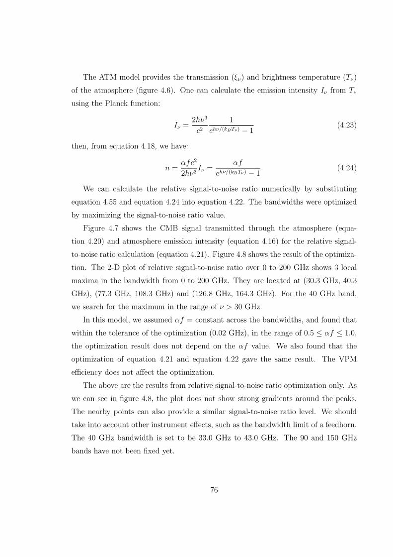
The ATM model provides the transmission (ξν) and brightness temperature (Tν)
of the atmosphere (figure 4.6). One can calculate the emission intensity Iν from Tν
using the Planck function:
Iν =2hν3
c21
ehν/(kBTν) − 1(4.23)
then, from equation 4.18, we have:
n =αfc2
2hν3Iν =
αf
ehν/(kBTν) − 1. (4.24)
We can calculate the relative signal-to-noise ratio numerically by substituting
equation 4.55 and equation 4.24 into equation 4.22. The bandwidths were optimized
by maximizing the signal-to-noise ratio value.
Figure 4.7 shows the CMB signal transmitted through the atmosphere (equa-
tion 4.20) and atmosphere emission intensity (equation 4.16) for the relative signal-
to-noise ratio calculation (equation 4.21). Figure 4.8 shows the result of the optimiza-
tion. The 2-D plot of relative signal-to-noise ratio over 0 to 200 GHz shows 3 local
maxima in the bandwidth from 0 to 200 GHz. They are located at (30.3 GHz, 40.3
GHz), (77.3 GHz, 108.3 GHz) and (126.8 GHz, 164.3 GHz). For the 40 GHz band,
we search for the maximum in the range of ν > 30 GHz.
In this model, we assumed αf = constant across the bandwidths, and found that
within the tolerance of the optimization (0.02 GHz), in the range of 0.5 ≤ αf ≤ 1.0,
the optimization result does not depend on the αf value. We also found that the
optimization of equation 4.21 and equation 4.22 gave the same result. The VPM
efficiency does not affect the optimization.
The above are the results from relative signal-to-noise ratio optimization only. As
we can see in figure 4.8, the plot does not show strong gradients around the peaks.
The nearby points can also provide a similar signal-to-noise ratio level. We should
take into account other instrument effects, such as the bandwidth limit of a feedhorn.
The 40 GHz bandwidth is set to be 33.0 GHz to 43.0 GHz. The 90 and 150 GHz
bands have not been fixed yet.
76
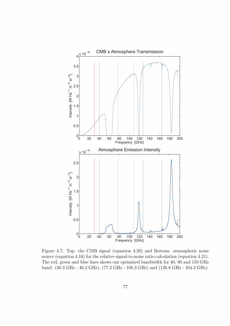
0 20 40 60 80 100 120 140 160 180 2000
0.5
1
1.5
2
2.5
3
3.5
4 x 10⁻¹⁸
Frequency [GHz]
Inte
nsity
[W
Hz−1
m−2
sr−2
]
CMB x Atmosphere Transmission
0 20 40 60 80 100 120 140 160 180 2000
0.5
1
1.5
2
2.5
x 10−15
Frequency [GHz]
Inte
nsity
[W
Hz−1
m−2
sr−2
]
Atmosphere Emission Intensity
Figure 4.7: Top: the CMB signal (equation 4.20) and Bottom: atmospheric noisesource (equation 4.16) for the relative signal-to-noise ratio calculation (equation 4.21).The red, green and blue lines shows our optimized bandwidth for 40, 90 and 150 GHzband: (30.3 GHz - 40.3 GHz), (77.3 GHz - 108.3 GHz) and (126.8 GHz - 164.3 GHz).
77
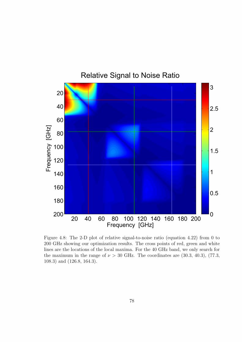
Frequency [GHz]
Freq
uenc
y [G
Hz]
Relative Signal to Noise Ratio
20 40 60 80 100 120 140 160 180 200
20
40
60
80
100
120
140
160
180
200 0
0.5
1
1.5
2
2.5
3
Figure 4.8: The 2-D plot of relative signal-to-noise ratio (equation 4.22) from 0 to200 GHz showing our optimization results. The cross points of red, green and whitelines are the locations of the local maxima. For the 40 GHz band, we only search forthe maximum in the range of ν > 30 GHz. The coordinates are (30.3, 40.3), (77.3,108.3) and (126.8, 164.3).
78
V (circular)
U
Q
HWP VPM
V (circular)
U
Q
Figure 4.9: As shown in Poincare sphere, VPM modulates between Q and V , whilethe HWP mix Q and U . In the case of VPM, the residuals due to the spectral effects(shown in blue) are a function of measurable modulation parameters. Figure courtesyof David Chuss.
4.3 The Variable-delay Polarization Modulator
VPM is the the first element of CLASS instrument. It modulates the sky polar-
ization signal by introducing a controlled variable path difference between two or-
thogonal linear polarizations of the incident radiation. Compared to the conventional
spinning Half Wave Plate (HWP), the advantages of the VPM can be summarized
as follows: [148] (1) The VPM is used in reflection, eliminating the effects from the
dielectrics (e.g., nonuniformity, birefringence, ...); (2) The VPM modulation employs
small motions, making it easier to achieve rapid modulation; (3) The VPM has more
flexibility in size than the HWP. This allows larger apertures that enable front-end
modulators for low frequency systems; (4) The modulation symmetry of the VPM
allows spectro-polarimetry; (5) The VPM does not convert between Stokes Q and U,
as opposed to the HWP (figure 4.9).
79
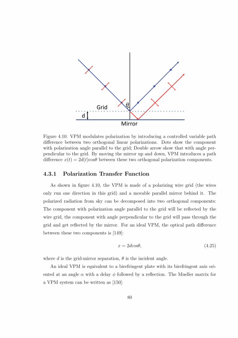
d
Mirror
Grid
Figure 4.10: VPM modulates polarization by introducing a controlled variable pathdifference between two orthogonal linear polarizations. Dots show the componentwith polarization angle parallel to the grid; Double arrow show that with angle per-pendicular to the grid. By moving the mirror up and down, VPM introduces a pathdifference x(t) = 2d(t)cosθ between these two orthogonal polarization components.
4.3.1 Polarization Transfer Function
As shown in figure 4.10, the VPM is made of a polarizing wire grid (the wires
only run one direction in this grid) and a movable parallel mirror behind it. The
polarized radiation from sky can be decomposed into two orthogonal components:
The component with polarization angle parallel to the grid will be reflected by the
wire grid, the component with angle perpendicular to the grid will pass through the
grid and get reflected by the mirror. For an ideal VPM, the optical path difference
between these two components is [149]:
x = 2dcosθ, (4.25)
where d is the grid-mirror separation, θ is the incident angle.
An ideal VPM is equivalent to a birefringent plate with its birefringent axis ori-
ented at an angle α with a delay φ followed by a reflection. The Mueller matrix for
a VPM system can be written as [150]:
80
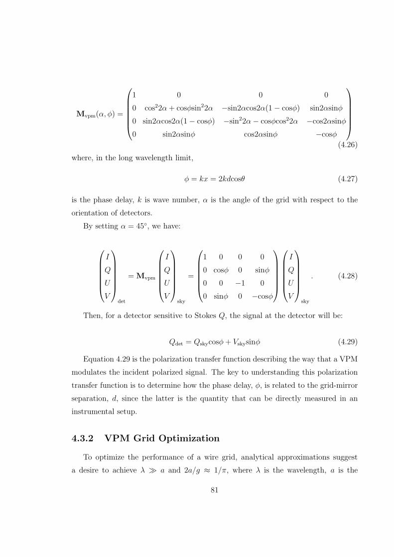
Mvpm(α, φ) =
1 0 0 0
0 cos22α+ cosφsin22α −sin2αcos2α(1− cosφ) sin2αsinφ
0 sin2αcos2α(1− cosφ) −sin22α− cosφcos22α −cos2αsinφ
0 sin2αsinφ cos2αsinφ −cosφ
(4.26)
where, in the long wavelength limit,
φ = kx = 2kdcosθ (4.27)
is the phase delay, k is wave number, α is the angle of the grid with respect to the
orientation of detectors.
By setting α = 45, we have:
I
Q
U
V
det
= Mvpm
I
Q
U
V
sky
=
1 0 0 0
0 cosφ 0 sinφ
0 0 −1 0
0 sinφ 0 −cosφ
I
Q
U
V
sky
. (4.28)
Then, for a detector sensitive to Stokes Q, the signal at the detector will be:
Qdet = Qskycosφ+ Vskysinφ (4.29)
Equation 4.29 is the polarization transfer function describing the way that a VPM
modulates the incident polarized signal. The key to understanding this polarization
transfer function is to determine how the phase delay, φ, is related to the grid-mirror
separation, d, since the latter is the quantity that can be directly measured in an
instrumental setup.
4.3.2 VPM Grid Optimization
To optimize the performance of a wire grid, analytical approximations suggest
a desire to achieve λ ≫ a and 2a/g ≈ 1/π, where λ is the wavelength, a is the
81
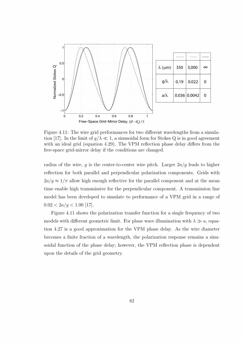
Figure 4.11: The wire grid performances for two different wavelengths from a simula-tion [17]. In the limit of g/λ≪ 1, a sinusoidal form for Stokes Q is in good agreementwith an ideal grid (equation 4.29). The VPM reflection phase delay differs from thefree-space grid-mirror delay if the conditions are changed.
radius of the wire, g is the center-to-center wire pitch. Larger 2a/g leads to higher
reflection for both parallel and perpendicular polarization components. Grids with
2a/g ≈ 1/π allow high enough reflective for the parallel component and at the mean
time enable high transmissive for the perpendicular component. A transmission line
model has been developed to simulate to performance of a VPM grid in a range of
0.02 < 2a/g < 1.00 [17].
Figure 4.11 shows the polarization transfer function for a single frequency of two
models with different geometric limit. For plane wave illumination with λ≫ a, equa-
tion 4.27 is a good approximation for the VPM phase delay. As the wire diameter
becomes a finite fraction of a wavelength, the polarization response remains a sinu-
soidal function of the phase delay; however, the VPM reflection phase is dependent
upon the details of the grid geometry.
82
4.3.3 VPM Mirror Throw Optimization
In the above discussion, a VPM grid with λ≫ a and 2a/g ≈ 1/π is a reasonable
approximation to an ideal VPM. This section will focus on the optimization of the
mirror throw for an ideal VPM base on maximizing the signal-to-noise ratio of its
output.
From equation 4.29, for a given bandpass kl to kh, the average output signal of an
ideal VPM as a function of x is:
S(x) =1
2(kh − kl)
∫ kh
kl
[I(k) +Q(k)cos(kx) + V (k)sin(kx)]dk (4.30)
where, I(k), Q(k), V (k) are the stokes parameters of the incident signal from the sky,
kl and kh are the wave numbers of the lower and higher limit of the waveband.
In CLASS wavebands, the atmospheric transmission is high and roughly constant
(figure 4.6), thus I(k), Q(k) and V (k) can be fit by a black body spectrum (∝AΩBν(T )):
I(k) = I0k
ehν/(kBTcmb) − 1=
I0k
eAk − 1
Q(k) = Q0k
ehν/(kBTcmb) − 1=
Q0k
eAk − 1
V (k) = V0k
ehν/(kBTcmb) − 1=
V0k
eAk − 1(4.31)
where, I0, Q0, V0 are constants and A = hc/(2πkBTcmb).
Then, equation 4.30 can be written as:
S(x) =1
2(kh − kl)
∫ kh
kl
[
I0k
eAk − 1+
Q0k
eAk − 1cos(kx) +
V0k
eAk − 1sin(kx)
]
dk
= SI × I0 + SQ(x)×Q0 + SV (x)× V0 (4.32)
83
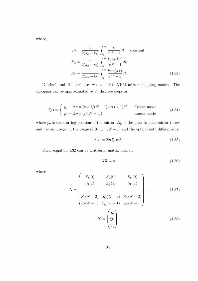
where,
SI =1
2(kh − kl)
∫ kh
kl
k
eAk − 1dk = constant
SQ =1
2(kh − kl)
∫ kh
kl
kcos(kx)
eAk − 1dk
SV =1
2(kh − kl)
∫ kh
kl
ksin(kx)
eAk − 1dk. (4.33)
“Cosine” and “Linear” are two candidate VPM mirror chopping modes. The
chopping can be approximated by N discrete steps as:
d(i) =
p0 +∆p× (cos(i/(N − 1) ∗ π) + 1)/2 Cosine mode
p0 +∆p× (i/(N − 1)) Linear mode(4.34)
where p0 is the starting position of the mirror, ∆p is the peak-to-peak mirror throw
and i is an integer in the range of (0, 1, ..., N − 1) and the optical path difference is:
x(i) = 2d(i)cosθ (4.35)
Then, equation 4.32 can be written in matrix format:
AX = s (4.36)
where
A =
SI(0) SQ(0) SV (0)
SI(1) SQ(1) SV (1)
... ... ...
SI(N − 2) SQ(N − 2) SV (N − 2)
SI(N − 1) SQ(N − 1) SV (N − 1)
, (4.37)
X =
I0
Q0
V0
(4.38)
84
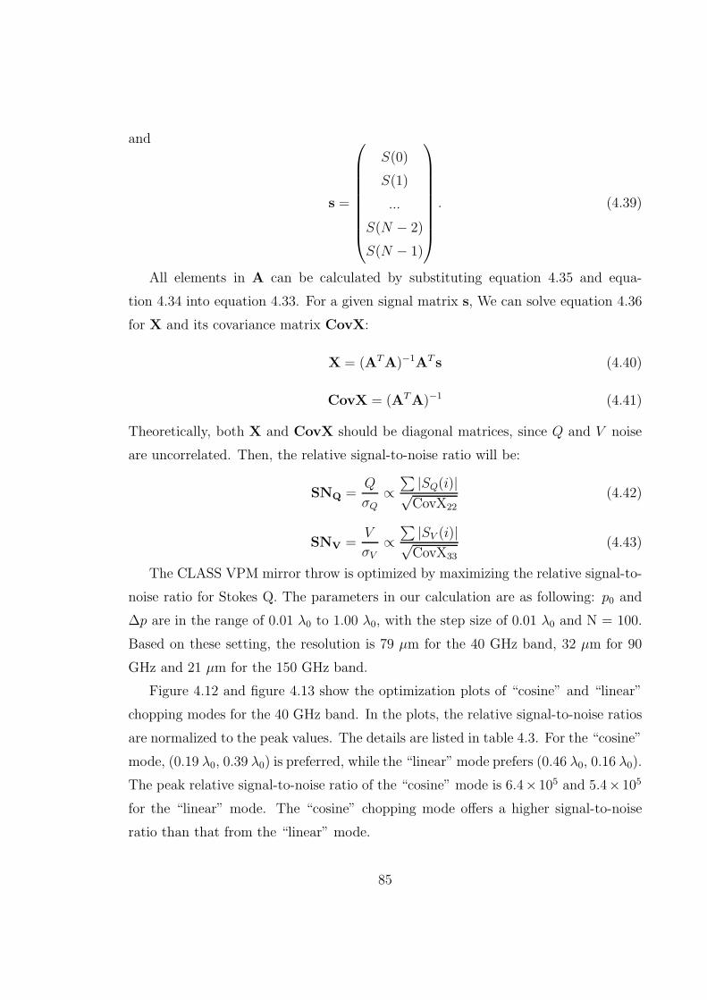
and
s =
S(0)
S(1)
...
S(N − 2)
S(N − 1)
. (4.39)
All elements in A can be calculated by substituting equation 4.35 and equa-
tion 4.34 into equation 4.33. For a given signal matrix s, We can solve equation 4.36
for X and its covariance matrix CovX:
X = (ATA)−1AT s (4.40)
CovX = (ATA)−1 (4.41)
Theoretically, both X and CovX should be diagonal matrices, since Q and V noise
are uncorrelated. Then, the relative signal-to-noise ratio will be:
SNQ =Q
σQ∝
∑ |SQ(i)|√CovX22
(4.42)
SNV =V
σV∝
∑
|SV (i)|√CovX33
(4.43)
The CLASS VPM mirror throw is optimized by maximizing the relative signal-to-
noise ratio for Stokes Q. The parameters in our calculation are as following: p0 and
∆p are in the range of 0.01 λ0 to 1.00 λ0, with the step size of 0.01 λ0 and N = 100.
Based on these setting, the resolution is 79 µm for the 40 GHz band, 32 µm for 90
GHz and 21 µm for the 150 GHz band.
Figure 4.12 and figure 4.13 show the optimization plots of “cosine” and “linear”
chopping modes for the 40 GHz band. In the plots, the relative signal-to-noise ratios
are normalized to the peak values. The details are listed in table 4.3. For the “cosine”
mode, (0.19 λ0, 0.39 λ0) is preferred, while the “linear” mode prefers (0.46 λ0, 0.16 λ0).
The peak relative signal-to-noise ratio of the “cosine” mode is 6.4×10⁵ and 5.4×10⁵
for the “linear” mode. The “cosine” chopping mode offers a higher signal-to-noise
ratio than that from the “linear” mode.
85
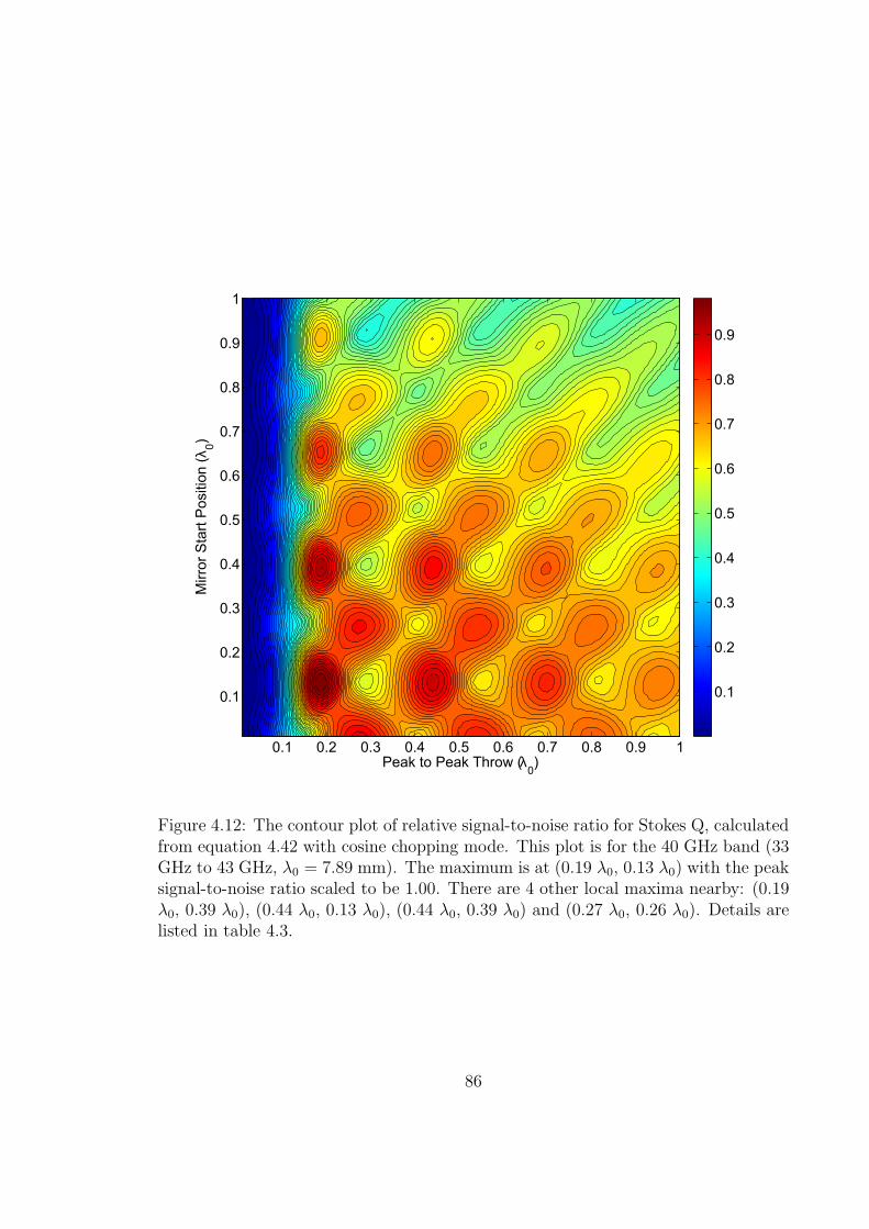
Peak to Peak Throw (λ0)
Mirr
or S
tart
Pos
ition
(λ0)
0.1 0.2 0.3 0.4 0.5 0.6 0.7 0.8 0.9 1
0.1
0.2
0.3
0.4
0.5
0.6
0.7
0.8
0.9
1
0.1
0.2
0.3
0.4
0.5
0.6
0.7
0.8
0.9
Figure 4.12: The contour plot of relative signal-to-noise ratio for Stokes Q, calculatedfrom equation 4.42 with cosine chopping mode. This plot is for the 40 GHz band (33GHz to 43 GHz, λ0 = 7.89 mm). The maximum is at (0.19 λ0, 0.13 λ0) with the peaksignal-to-noise ratio scaled to be 1.00. There are 4 other local maxima nearby: (0.19λ0, 0.39 λ0), (0.44 λ0, 0.13 λ0), (0.44 λ0, 0.39 λ0) and (0.27 λ0, 0.26 λ0). Details arelisted in table 4.3.
86
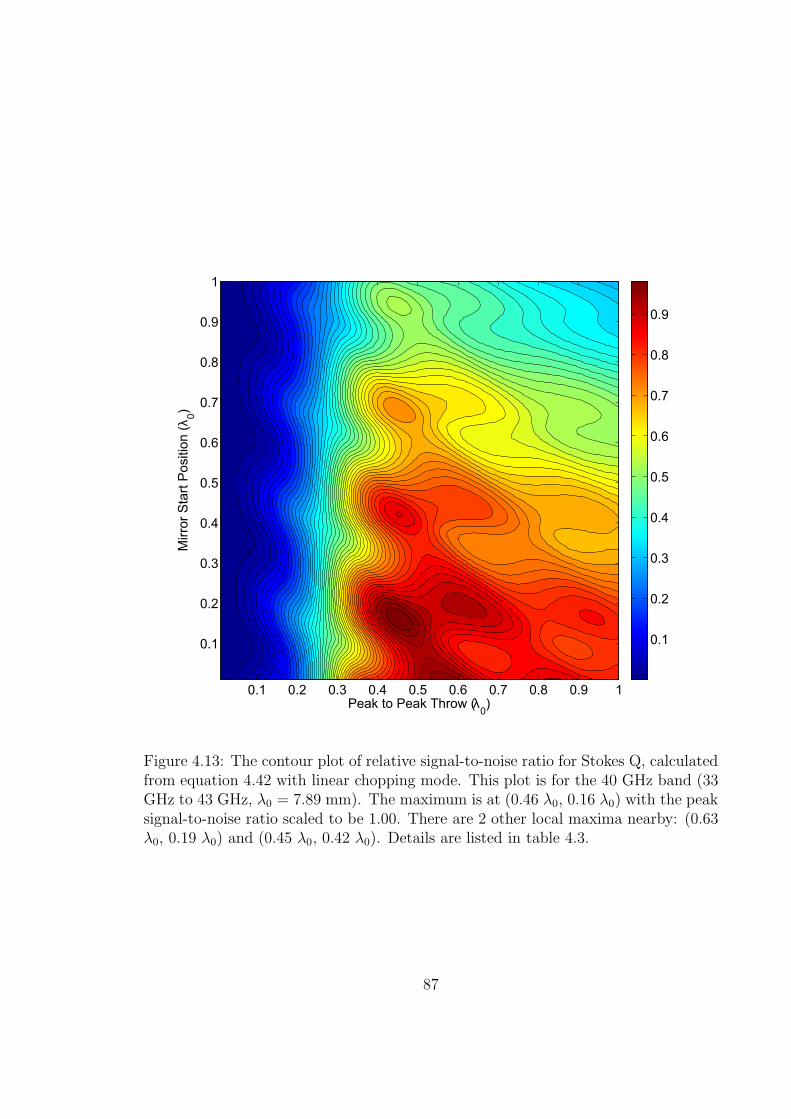
Peak to Peak Throw (λ0)
Mirr
or S
tart
Pos
ition
(λ0)
0.1 0.2 0.3 0.4 0.5 0.6 0.7 0.8 0.9 1
0.1
0.2
0.3
0.4
0.5
0.6
0.7
0.8
0.9
1
0.1
0.2
0.3
0.4
0.5
0.6
0.7
0.8
0.9
Figure 4.13: The contour plot of relative signal-to-noise ratio for Stokes Q, calculatedfrom equation 4.42 with linear chopping mode. This plot is for the 40 GHz band (33GHz to 43 GHz, λ0 = 7.89 mm). The maximum is at (0.46 λ0, 0.16 λ0) with the peaksignal-to-noise ratio scaled to be 1.00. There are 2 other local maxima nearby: (0.63λ0, 0.19 λ0) and (0.45 λ0, 0.42 λ0). Details are listed in table 4.3.
87
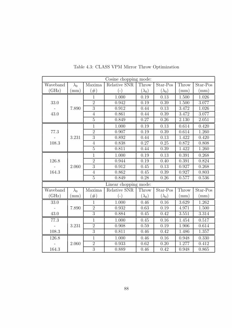
Table 4.3: CLASS VPM Mirror Throw Optimization
Cosine chopping mode:Waveband λ0 Maxima Relative SNR Throw Star-Pos Throw Star-Pos(GHz) (mm) (#) (-) (λ0) (λ0) (mm) (mm)
7.890
1 1.000 0.19 0.13 1.500 1.02633.0 2 0.942 0.19 0.39 1.500 3.077- 3 0.912 0.44 0.13 3.472 1.026
43.0 4 0.861 0.44 0.39 3.472 3.0775 0.849 0.27 0.26 2.130 2.051
3.231
1 1.000 0.19 0.13 0.614 0.42077.3 2 0.907 0.19 0.39 0.614 1.260- 3 0.892 0.44 0.13 1.422 0.420
108.3 4 0.838 0.27 0.25 0.872 0.8085 0.811 0.44 0.39 1.422 1.260
2.060
1 1.000 0.19 0.13 0.391 0.268126.8 2 0.944 0.19 0.40 0.391 0.824- 3 0.912 0.45 0.13 0.927 0.268
164.3 4 0.862 0.45 0.39 0.927 0.8035 0.849 0.28 0.26 0.577 0.536
Linear chopping mode:Waveband λ0 Maxima Relative SNR Throw Star-Pos Throw Star-Pos(GHz) (mm) (#) (-) (λ0) (λ0) (mm) (mm)
33.07.890
1 1.000 0.46 0.16 3.629 1.262- 2 0.932 0.63 0.19 4.971 1.500
43.0 3 0.884 0.45 0.42 3.551 3.314
77.33.231
1 1.000 0.45 0.16 1.454 0.517- 2 0.908 0.59 0.19 1.906 0.614
108.3 3 0.811 0.46 0.42 1.486 1.357
126.82.060
1 1.000 0.46 0.16 0.948 0.330- 2 0.933 0.62 0.20 1.277 0.412
164.3 3 0.889 0.46 0.42 0.948 0.865
88
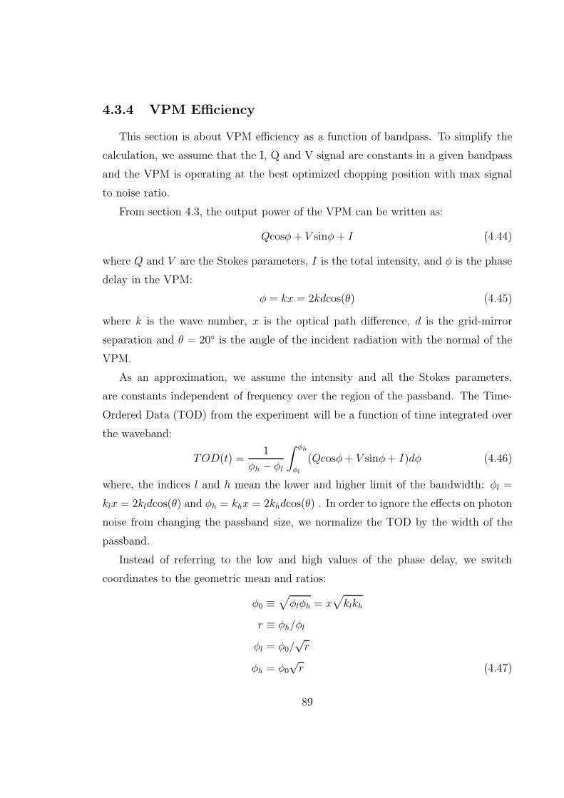
4.3.4 VPM Efficiency
This section is about VPM efficiency as a function of bandpass. To simplify the
calculation, we assume that the I, Q and V signal are constants in a given bandpass
and the VPM is operating at the best optimized chopping position with max signal
to noise ratio.
From section 4.3, the output power of the VPM can be written as:
Qcosφ+ V sinφ+ I (4.44)
where Q and V are the Stokes parameters, I is the total intensity, and φ is the phase
delay in the VPM:
φ = kx = 2kdcos(θ) (4.45)
where k is the wave number, x is the optical path difference, d is the grid-mirror
separation and θ = 20 is the angle of the incident radiation with the normal of the
VPM.
As an approximation, we assume the intensity and all the Stokes parameters,
are constants independent of frequency over the region of the passband. The Time-
Ordered Data (TOD) from the experiment will be a function of time integrated over
the waveband:
TOD(t) =1
φh − φl
∫ φh
φl
(Qcosφ+ V sinφ+ I)dφ (4.46)
where, the indices l and h mean the lower and higher limit of the bandwidth: φl =
klx = 2kldcos(θ) and φh = khx = 2khdcos(θ) . In order to ignore the effects on photon
noise from changing the passband size, we normalize the TOD by the width of the
passband.
Instead of referring to the low and high values of the phase delay, we switch
coordinates to the geometric mean and ratios:
φ0 ≡√
φlφh = x√
klkh
r ≡ φh/φl
φl = φ0/√r
φh = φ0
√r (4.47)
89
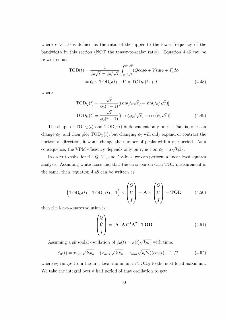
where r > 1.0 is defined as the ratio of the upper to the lower frequency of the
bandwidth in this section (NOT the tensor-to-scalar ratio). Equation 4.46 can be
re-written as:
TOD(t) =1
φ0
√r − φ0/
√r
∫ φ0√r
φ0/√r
(Qcosφ+ V sinφ+ I)dφ
= Q× TODQ(t) + V × TODV (t) + I (4.48)
where
TODQ(t) =
√r
φ0(r − 1)[(sin(φ0
√r)− sin(φ0/
√r)]
TODV (t) =
√r
φ0(r − 1)[(cos(φ0/
√r)− cos(φ0
√r)]. (4.49)
The shape of TODQ(t) and TODV (t) is dependent only on r. That is, one can
change φ0, and then plot TODQ(t), but changing φ0 will only expand or contract the
horizontal direction, it won’t change the number of peaks within one period. As a
consequence, the VPM efficiency depends only on r, not on φ0 = x√klkh.
In order to solve for the Q, V , and I values, we can perform a linear least squares
analysis. Assuming white noise and that the error bar on each TOD measurement is
the same, then, equation 4.48 can be written as:
(
TODQ(t), TODV (t), 1)
×
Q
V
I
= A×
Q
V
I
= TOD (4.50)
then the least-squares solution is:
Q
V
I
= (ATA)−1AT ·TOD (4.51)
Assuming a sinsoidal oscillation of φ0(t) = x(t)√klkh with time:
φ0(t) = xmin
√
klkh + (xmax
√
klkh − xmin
√
klkh)(cos(t) + 1)/2 (4.52)
where φ0 ranges from the first local minimum in TODQ to the next local maximum.
We take the integral over a half period of that oscillation to get:
90
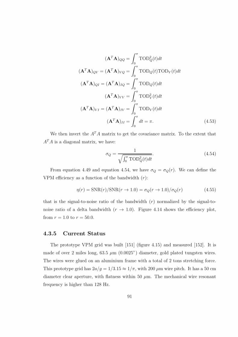
(ATA)QQ =
∫ π
0
TOD2Q(t)dt
(ATA)QV = (ATA)V Q =
∫ π
0
TODQ(t)TODV (t)dt
(ATA)QI = (ATA)IQ =
∫ π
0
TODQ(t)dt
(ATA)V V =
∫ π
0
TOD2V (t)dt
(ATA)V I = (ATA)IV =
∫ π
0
TODV (t)dt
(ATA)II =
∫ π
0
dt = π. (4.53)
We then invert the ATA matrix to get the covariance matrix. To the extent that
ATA is a diagonal matrix, we have:
σQ =1
√
∫ π
0TOD2
Q(t)dt. (4.54)
From equation 4.49 and equation 4.54, we have σQ = σQ(r). We can define the
VPM efficiency as a function of the bandwidth (r):
η(r) = SNR(r)/SNR(r → 1.0) = σQ(r → 1.0)/σQ(r) (4.55)
that is the signal-to-noise ratio of the bandwidth (r) normalized by the signal-to-
noise ratio of a delta bandwidth (r → 1.0). Figure 4.14 shows the efficiency plot,
from r = 1.0 to r = 50.0.
4.3.5 Current Status
The prototype VPM grid was built [151] (figure 4.15) and measured [152]. It is
made of over 2 miles long, 63.5 µm (0.0025”) diameter, gold plated tungsten wires.
The wires were glued on an aluminium frame with a total of 2 tons stretching force.
This prototype grid has 2a/g = 1/3.15 ≈ 1/π, with 200 µm wire pitch. It has a 50 cm
diameter clear aperture, with flatness within 50 µm. The mechanical wire resonant
frequency is higher than 128 Hz.
91
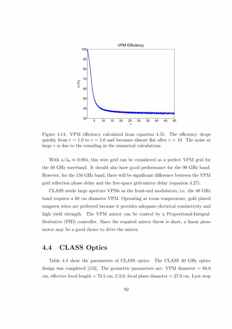
5 10 15 20 25 30 35 40 45 5030
40
50
60
70
80
90
100VPM Efficiency
r
η (%
)
Figure 4.14: VPM efficiency calculated from equation 4.55. The efficiency dropsquickly from r = 1.0 to r = 5.0 and becomes almost flat after r > 10. The noise atlarge r is due to the rounding in the numerical calculations.
With a/λ0 ≈ 0.004, this wire grid can be considered as a perfect VPM grid for
the 40 GHz waveband. It should also have good performance for the 90 GHz band.
However, for the 150 GHz band, there will be significant difference between the VPM
grid reflection phase delay and the free-space grid-mirror delay (equation 4.27).
CLASS needs large aperture VPMs as the front-end modulators, i.e. the 40 GHz
band requires a 60 cm diameter VPM. Operating at room temperature, gold plated
tungsten wires are preferred because it provides adequate electrical conductivity and
high yield strength. The VPM mirror can be control by a Proportional-Integral-
Derivative (PID) controller. Since the required mirror throw is short, a linear piezo
motor may be a good choice to drive the mirror.
4.4 CLASS Optics
Table 4.4 show the parameters of CLASS optics. The CLASS 40 GHz optics
design was completed [153]. The geometric parameters are: VPM diameter = 60.0
cm, effective focal length = 70.5 cm, f/2.0, focal plane diameter = 27.0 cm, Lyot stop
92
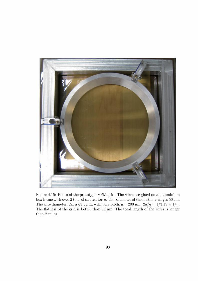
Figure 4.15: Photo of the prototype VPM grid. The wires are glued on an aluminiumbox frame with over 2 tons of stretch force. The diameter of the flattener ring is 50 cm.The wire diameter, 2a, is 63.5 µm, with wire pitch, g = 200 µm. 2a/g = 1/3.15 ≈ 1/π.The flatness of the grid is better than 50 µm. The total length of the wires is longerthan 2 miles.
93
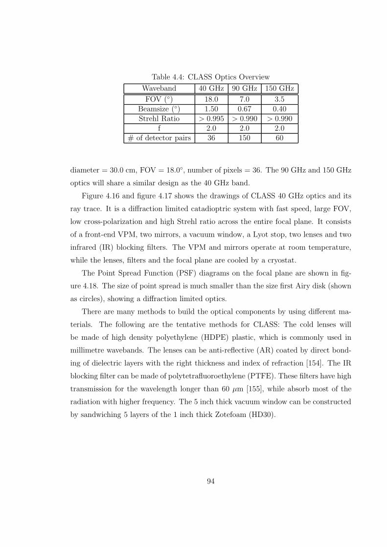
Table 4.4: CLASS Optics Overview
Waveband 40 GHz 90 GHz 150 GHz
FOV () 18.0 7.0 3.5Beamsize () 1.50 0.67 0.40Strehl Ratio > 0.995 > 0.990 > 0.990
f 2.0 2.0 2.0# of detector pairs 36 150 60
diameter = 30.0 cm, FOV = 18.0, number of pixels = 36. The 90 GHz and 150 GHz
optics will share a similar design as the 40 GHz band.
Figure 4.16 and figure 4.17 shows the drawings of CLASS 40 GHz optics and its
ray trace. It is a diffraction limited catadioptric system with fast speed, large FOV,
low cross-polarization and high Strehl ratio across the entire focal plane. It consists
of a front-end VPM, two mirrors, a vacuum window, a Lyot stop, two lenses and two
infrared (IR) blocking filters. The VPM and mirrors operate at room temperature,
while the lenses, filters and the focal plane are cooled by a cryostat.
The Point Spread Function (PSF) diagrams on the focal plane are shown in fig-
ure 4.18. The size of point spread is much smaller than the size first Airy disk (shown
as circles), showing a diffraction limited optics.
There are many methods to build the optical components by using different ma-
terials. The following are the tentative methods for CLASS: The cold lenses will
be made of high density polyethylene (HDPE) plastic, which is commonly used in
millimetre wavebands. The lenses can be anti-reflective (AR) coated by direct bond-
ing of dielectric layers with the right thickness and index of refraction [154]. The IR
blocking filter can be made of polytetrafluoroethylene (PTFE). These filters have high
transmission for the wavelength longer than 60 µm [155], while absorb most of the
radiation with higher frequency. The 5 inch thick vacuum window can be constructed
by sandwiching 5 layers of the 1 inch thick Zotefoam (HD30).
94
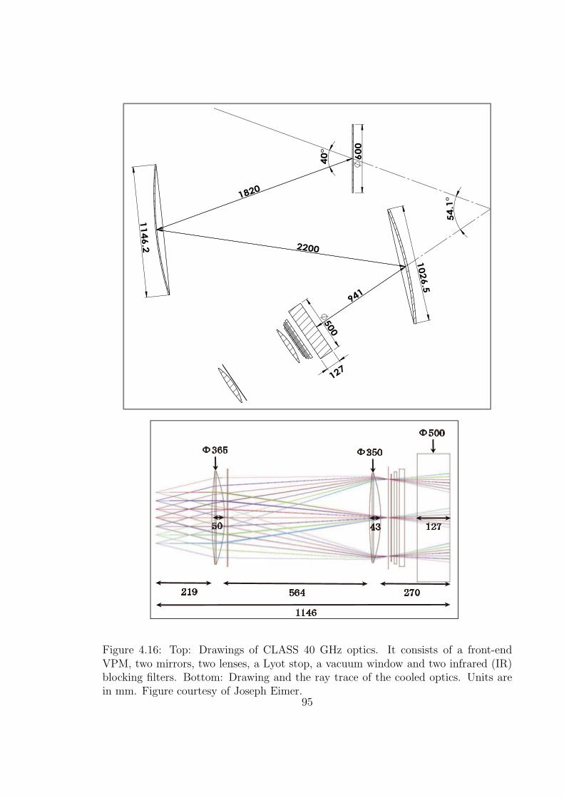
600
500
127
1026.5
1146.2
1820
2200
40°
54.1°
941
Figure 4.16: Top: Drawings of CLASS 40 GHz optics. It consists of a front-endVPM, two mirrors, two lenses, a Lyot stop, a vacuum window and two infrared (IR)blocking filters. Bottom: Drawing and the ray trace of the cooled optics. Units arein mm. Figure courtesy of Joseph Eimer.
95
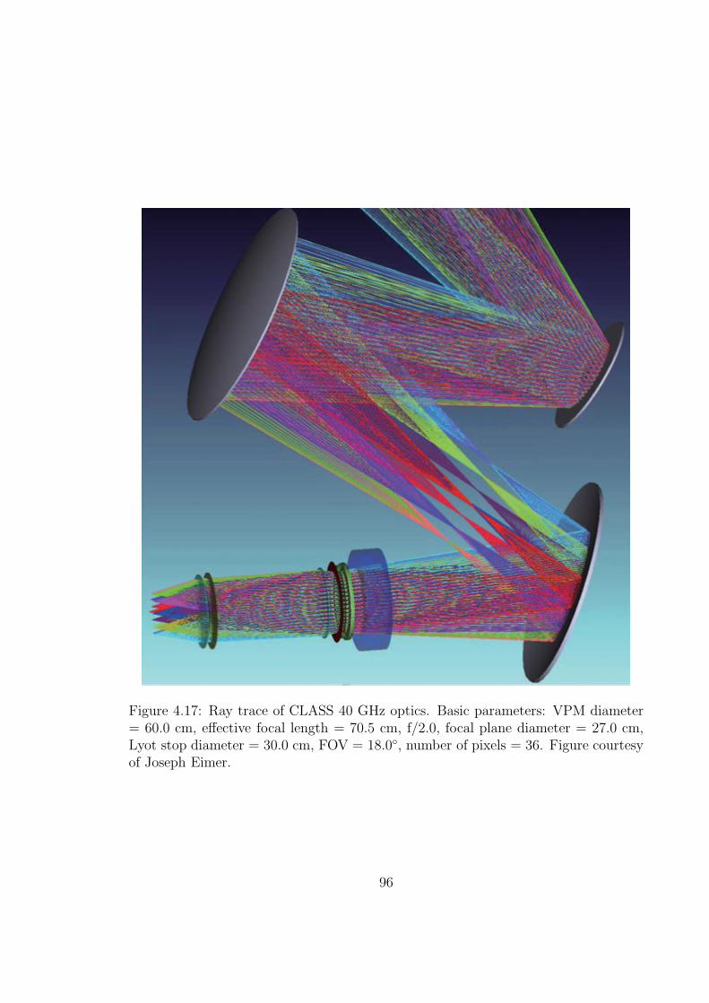
Figure 4.17: Ray trace of CLASS 40 GHz optics. Basic parameters: VPM diameter= 60.0 cm, effective focal length = 70.5 cm, f/2.0, focal plane diameter = 27.0 cm,Lyot stop diameter = 30.0 cm, FOV = 18.0, number of pixels = 36. Figure courtesyof Joseph Eimer.
96
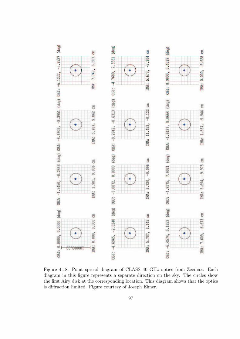
Figure 4.18: Point spread diagram of CLASS 40 GHz optics from Zeemax. Eachdiagram in this figure represents a separate direction on the sky. The circles showthe first Airy disk at the corresponding location. This diagram shows that the opticsis diffraction limited. Figure courtesy of Joseph Eimer.
97
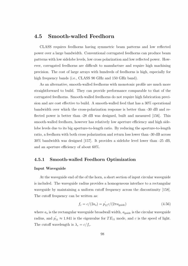
4.5 Smooth-walled Feedhorn
CLASS requires feedhorns having symmetric beam patterns and low reflected
power over a large bandwidth. Conventional corrugated feedhorns can produce beam
patterns with low sidelobe levels, low cross polarization and low reflected power. How-
ever, corrugated feedhorns are difficult to manufacture and require high machining
precision. The cost of large arrays with hundreds of feedhorns is high, especially for
high frequency bands (i.e., CLASS 90 GHz and 150 GHz band).
As an alternative, smooth-walled feedhorns with monotonic profile are much more
straightforward to build. They can provide performance comparable to that of the
corrugated feedhorns. Smooth-walled feedhorns do not require high fabrication preci-
sion and are cost effective to build. A smooth-walled feed that has a 30% operational
bandwidth over which the cross-polarization response is better than -30 dB and re-
flected power is better than -28 dB was designed, built and measured [156]. This
smooth-walled feedhorn, however has relatively low aperture efficiency and high side-
lobe levels due to its big aperture-to-length ratio. By reducing the aperture-to-length
ratio, a feedhorn with both cross polarization and return loss lower than -30 dB across
30% bandwidth was designed [157]. It provides a sidelobe level lower than -25 dB,
and an aperture efficiency of about 60%.
4.5.1 Smooth-walled Feedhorn Optimization
Input Waveguide
At the waveguide end of the of the horn, a short section of input circular waveguide
is included. The waveguide radius provides a homogeneous interface to a rectangular
waveguide by maintaining a uniform cutoff frequency across the discontinuity [158].
The cutoff frequency can be written as:
fc = c/(2ao) = p′
11c/(2πaguide) (4.56)
where ao is the rectangular waveguide broadwall width, aguide is the circular waveguide
radius, and p′
11 ≈ 1.841 is the eigenvalue for TE11 mode, and c is the speed of light.
The cutoff wavelength is λc = c/fc.
98
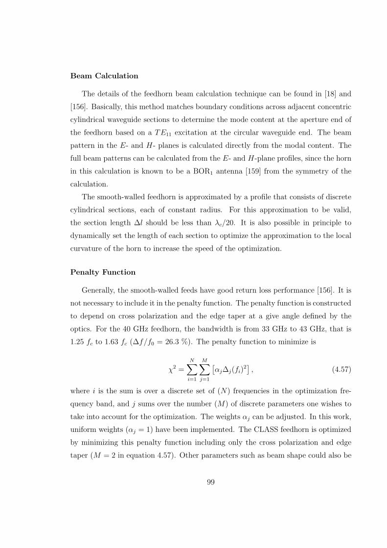
Beam Calculation
The details of the feedhorn beam calculation technique can be found in [18] and
[156]. Basically, this method matches boundary conditions across adjacent concentric
cylindrical waveguide sections to determine the mode content at the aperture end of
the feedhorn based on a TE11 excitation at the circular waveguide end. The beam
pattern in the E- and H- planes is calculated directly from the modal content. The
full beam patterns can be calculated from the E- and H-plane profiles, since the horn
in this calculation is known to be a BOR1 antenna [159] from the symmetry of the
calculation.
The smooth-walled feedhorn is approximated by a profile that consists of discrete
cylindrical sections, each of constant radius. For this approximation to be valid,
the section length ∆l should be less than λc/20. It is also possible in principle to
dynamically set the length of each section to optimize the approximation to the local
curvature of the horn to increase the speed of the optimization.
Penalty Function
Generally, the smooth-walled feeds have good return loss performance [156]. It is
not necessary to include it in the penalty function. The penalty function is constructed
to depend on cross polarization and the edge taper at a give angle defined by the
optics. For the 40 GHz feedhorn, the bandwidth is from 33 GHz to 43 GHz, that is
1.25 fc to 1.63 fc (∆f/f0 = 26.3 %). The penalty function to minimize is
χ2 =
N∑
i=1
M∑
j=1
[
αj∆j(fi)2]
, (4.57)
where i is the sum is over a discrete set of (N) frequencies in the optimization fre-
quency band, and j sums over the number (M) of discrete parameters one wishes to
take into account for the optimization. The weights αj can be adjusted. In this work,
uniform weights (αj = 1) have been implemented. The CLASS feedhorn is optimized
by minimizing this penalty function including only the cross polarization and edge
taper (M = 2 in equation 4.57). Other parameters such as beam shape could also be
99
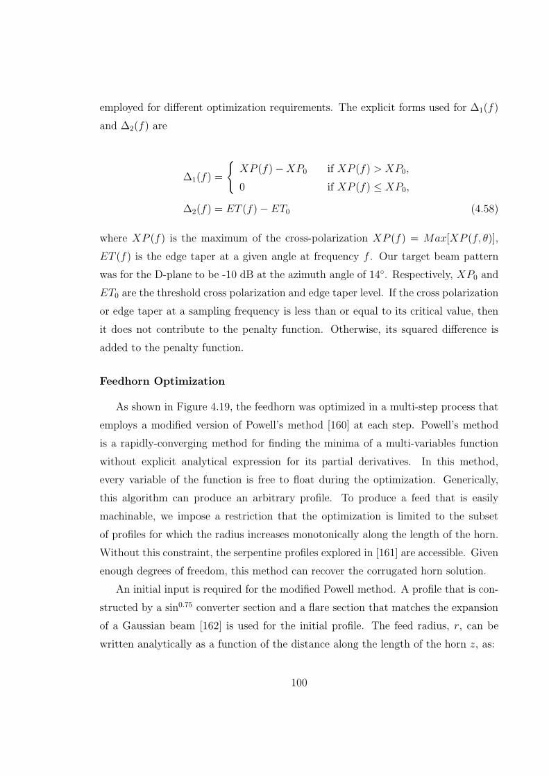
employed for different optimization requirements. The explicit forms used for ∆1(f)
and ∆2(f) are
∆1(f) =
XP (f)−XP0 if XP (f) > XP0,
0 if XP (f) ≤ XP0,
∆2(f) = ET (f)− ET0 (4.58)
where XP (f) is the maximum of the cross-polarization XP (f) = Max[XP (f, θ)],
ET (f) is the edge taper at a given angle at frequency f . Our target beam pattern
was for the D-plane to be -10 dB at the azimuth angle of 14. Respectively, XP0 and
ET0 are the threshold cross polarization and edge taper level. If the cross polarization
or edge taper at a sampling frequency is less than or equal to its critical value, then
it does not contribute to the penalty function. Otherwise, its squared difference is
added to the penalty function.
Feedhorn Optimization
As shown in Figure 4.19, the feedhorn was optimized in a multi-step process that
employs a modified version of Powell’s method [160] at each step. Powell’s method
is a rapidly-converging method for finding the minima of a multi-variables function
without explicit analytical expression for its partial derivatives. In this method,
every variable of the function is free to float during the optimization. Generically,
this algorithm can produce an arbitrary profile. To produce a feed that is easily
machinable, we impose a restriction that the optimization is limited to the subset
of profiles for which the radius increases monotonically along the length of the horn.
Without this constraint, the serpentine profiles explored in [161] are accessible. Given
enough degrees of freedom, this method can recover the corrugated horn solution.
An initial input is required for the modified Powell method. A profile that is con-
structed by a sin0.75 converter section and a flare section that matches the expansion
of a Gaussian beam [162] is used for the initial profile. The feed radius, r, can be
written analytically as a function of the distance along the length of the horn z, as:
100
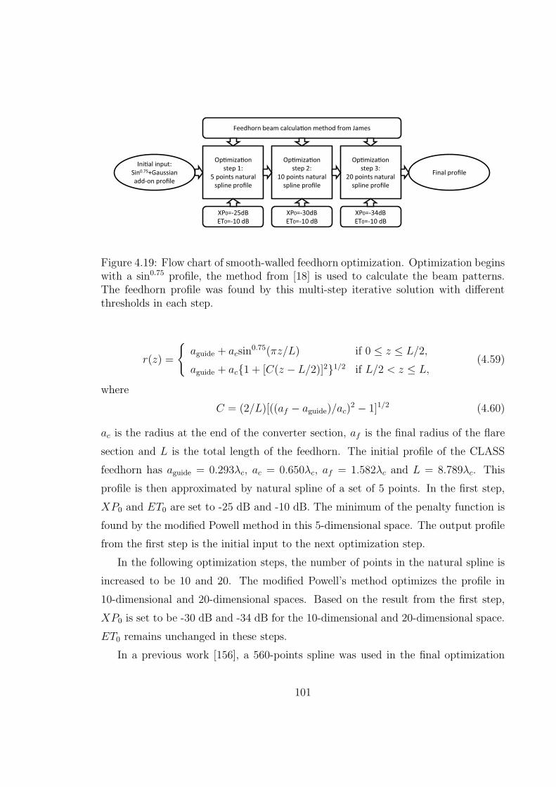
Inial input:
Sin0.75+Gaussian
add-on profile
XP0=-25dB
ET0=-10 dB
Feedhorn beam calculaon method from James
Opmizaon
step 1:
5 points natural
spline profile
Opmizaon
step 2:
10 points natural
spline profile
Opmizaon
step 3:
20 points natural
spline profile
Final profile
XP0=-30dB
ET0=-10 dB
XP0=-34dB
ET0=-10 dB
Figure 4.19: Flow chart of smooth-walled feedhorn optimization. Optimization beginswith a sin0.75 profile, the method from [18] is used to calculate the beam patterns.The feedhorn profile was found by this multi-step iterative solution with differentthresholds in each step.
r(z) =
aguide + acsin0.75(πz/L) if 0 ≤ z ≤ L/2,
aguide + ac1 + [C(z − L/2)]21/2 if L/2 < z ≤ L,(4.59)
where
C = (2/L)[((af − aguide)/ac)2 − 1]1/2 (4.60)
ac is the radius at the end of the converter section, af is the final radius of the flare
section and L is the total length of the feedhorn. The initial profile of the CLASS
feedhorn has aguide = 0.293λc, ac = 0.650λc, af = 1.582λc and L = 8.789λc. This
profile is then approximated by natural spline of a set of 5 points. In the first step,
XP0 and ET0 are set to -25 dB and -10 dB. The minimum of the penalty function is
found by the modified Powell method in this 5-dimensional space. The output profile
from the first step is the initial input to the next optimization step.
In the following optimization steps, the number of points in the natural spline is
increased to be 10 and 20. The modified Powell’s method optimizes the profile in
10-dimensional and 20-dimensional spaces. Based on the result from the first step,
XP0 is set to be -30 dB and -34 dB for the 10-dimensional and 20-dimensional space.
ET0 remains unchanged in these steps.
In a previous work [156], a 560-points spline was used in the final optimization
101
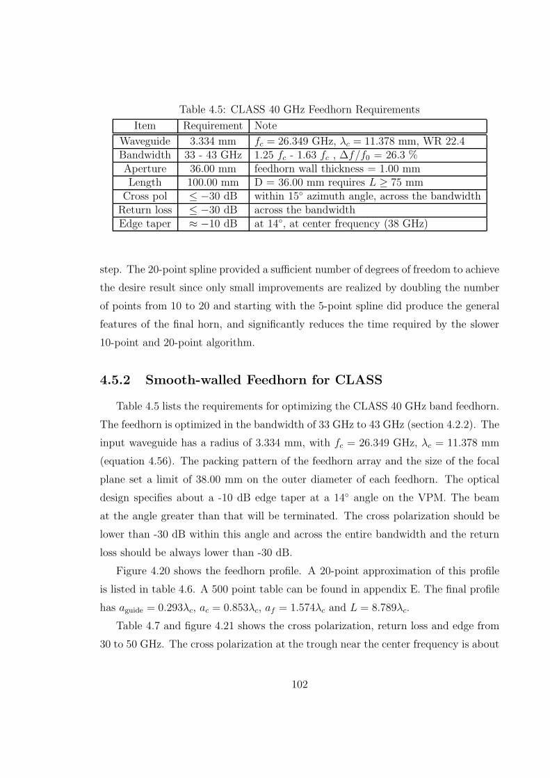
Table 4.5: CLASS 40 GHz Feedhorn Requirements
Item Requirement Note
Waveguide 3.334 mm fc = 26.349 GHz, λc = 11.378 mm, WR 22.4Bandwidth 33 - 43 GHz 1.25 fc - 1.63 fc , ∆f/f0 = 26.3 %Aperture 36.00 mm feedhorn wall thickness = 1.00 mmLength 100.00 mm D = 36.00 mm requires L ≥ 75 mm
Cross pol ≤ −30 dB within 15 azimuth angle, across the bandwidthReturn loss ≤ −30 dB across the bandwidthEdge taper ≈ −10 dB at 14, at center frequency (38 GHz)
step. The 20-point spline provided a sufficient number of degrees of freedom to achieve
the desire result since only small improvements are realized by doubling the number
of points from 10 to 20 and starting with the 5-point spline did produce the general
features of the final horn, and significantly reduces the time required by the slower
10-point and 20-point algorithm.
4.5.2 Smooth-walled Feedhorn for CLASS
Table 4.5 lists the requirements for optimizing the CLASS 40 GHz band feedhorn.
The feedhorn is optimized in the bandwidth of 33 GHz to 43 GHz (section 4.2.2). The
input waveguide has a radius of 3.334 mm, with fc = 26.349 GHz, λc = 11.378 mm
(equation 4.56). The packing pattern of the feedhorn array and the size of the focal
plane set a limit of 38.00 mm on the outer diameter of each feedhorn. The optical
design specifies about a -10 dB edge taper at a 14 angle on the VPM. The beam
at the angle greater than that will be terminated. The cross polarization should be
lower than -30 dB within this angle and across the entire bandwidth and the return
loss should be always lower than -30 dB.
Figure 4.20 shows the feedhorn profile. A 20-point approximation of this profile
is listed in table 4.6. A 500 point table can be found in appendix E. The final profile
has aguide = 0.293λc, ac = 0.853λc, af = 1.574λc and L = 8.789λc.
Table 4.7 and figure 4.21 shows the cross polarization, return loss and edge from
30 to 50 GHz. The cross polarization at the trough near the center frequency is about
102
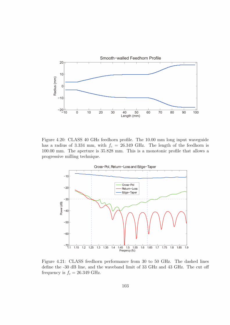
−10 0 10 20 30 40 50 60 70 80 90 100−20
−10
0
10
20Smooth−walled Feedhorn Profile
Length (mm)
Rad
ius
(mm
)
Figure 4.20: CLASS 40 GHz feedhorn profile. The 10.00 mm long input waveguidehas a radius of 3.334 mm, with fc = 26.349 GHz. The length of the feedhorn is100.00 mm. The aperture is 35.828 mm. This is a monotonic profile that allows aprogressive milling technique.
1.1 1.15 1.2 1.25 1.3 1.35 1.4 1.45 1.5 1.55 1.6 1.65 1.7 1.75 1.8 1.85 1.9−70
−60
−50
−40
−30
−20
−10
Cross−Pol, Return−Loss and Edge−Taper
Freqency (fc)
Pow
er (d
B)
Cross−PolReturn−LossEdge−Taper
Figure 4.21: CLASS feedhorn performance from 30 to 50 GHz. The dashed linesdefine the -30 dB line, and the waveband limit of 33 GHz and 43 GHz. The cut offfrequency is fc = 26.349 GHz.
103
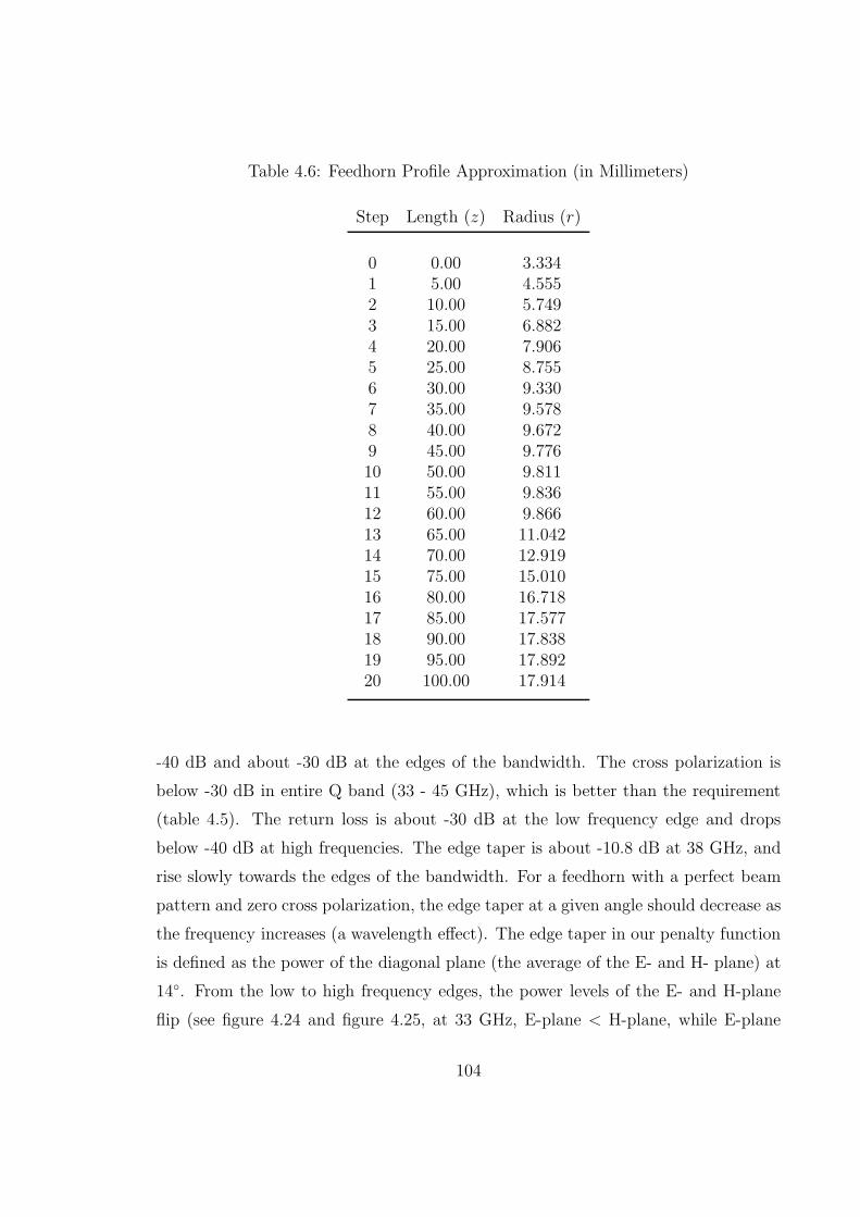
Table 4.6: Feedhorn Profile Approximation (in Millimeters)
Step Length (z) Radius (r)
0 0.00 3.3341 5.00 4.5552 10.00 5.7493 15.00 6.8824 20.00 7.9065 25.00 8.7556 30.00 9.3307 35.00 9.5788 40.00 9.6729 45.00 9.77610 50.00 9.81111 55.00 9.83612 60.00 9.86613 65.00 11.04214 70.00 12.91915 75.00 15.01016 80.00 16.71817 85.00 17.57718 90.00 17.83819 95.00 17.89220 100.00 17.914
-40 dB and about -30 dB at the edges of the bandwidth. The cross polarization is
below -30 dB in entire Q band (33 - 45 GHz), which is better than the requirement
(table 4.5). The return loss is about -30 dB at the low frequency edge and drops
below -40 dB at high frequencies. The edge taper is about -10.8 dB at 38 GHz, and
rise slowly towards the edges of the bandwidth. For a feedhorn with a perfect beam
pattern and zero cross polarization, the edge taper at a given angle should decrease as
the frequency increases (a wavelength effect). The edge taper in our penalty function
is defined as the power of the diagonal plane (the average of the E- and H- plane) at
14. From the low to high frequency edges, the power levels of the E- and H-plane
flip (see figure 4.24 and figure 4.25, at 33 GHz, E-plane < H-plane, while E-plane
104
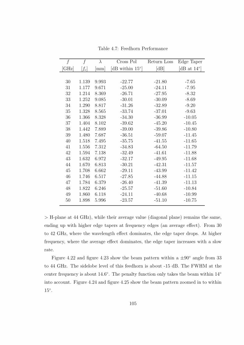
Table 4.7: Feedhorn Performance
f f λ Cross Pol Return Loss Edge Taper
[GHz] [fc] [mm] [dB within 15] [dB] [dB at 14]
30 1.139 9.993 -22.77 -21.80 -7.6531 1.177 9.671 -25.00 -24.11 -7.9532 1.214 8.369 -26.71 -27.95 -8.3233 1.252 9.085 -30.01 -30.09 -8.6934 1.290 8.817 -31.26 -32.89 -9.2035 1.328 8.565 -33.74 -37.01 -9.6336 1.366 8.328 -34.30 -36.99 -10.0537 1.404 8.102 -39.62 -45.20 -10.4538 1.442 7.889 -39.00 -39.86 -10.8039 1.480 7.687 -36.51 -59.07 -11.4540 1.518 7.495 -35.75 -41.55 -11.6541 1.556 7.312 -34.83 -64.50 -11.7942 1.594 7.138 -32.49 -41.61 -11.8843 1.632 6.972 -32.17 -49.95 -11.6844 1.670 6.813 -30.21 -42.31 -11.5745 1.708 6.662 -29.11 -43.99 -11.4246 1.746 6.517 -27.85 -44.88 -11.1547 1.784 6.379 -26.40 -41.39 -11.1348 1.822 6.246 -25.57 -51.60 -10.8449 1.860 6.118 -24.11 -40.68 -10.9950 1.898 5.996 -23.57 -51.10 -10.75
> H-plane at 44 GHz), while their average value (diagonal plane) remains the same,
ending up with higher edge tapers at frequency edges (an average effect). From 30
to 42 GHz, where the wavelength effect dominates, the edge taper drops. At higher
frequency, where the average effect dominates, the edge taper increases with a slow
rate.
Figure 4.22 and figure 4.23 show the beam pattern within a ±90 angle from 33
to 44 GHz. The sidelobe level of this feedhorn is about -15 dB. The FWHM at the
center frequency is about 14.6. The penalty function only takes the beam within 14
into account. Figure 4.24 and figure 4.25 show the beam pattern zoomed in to within
15.
105
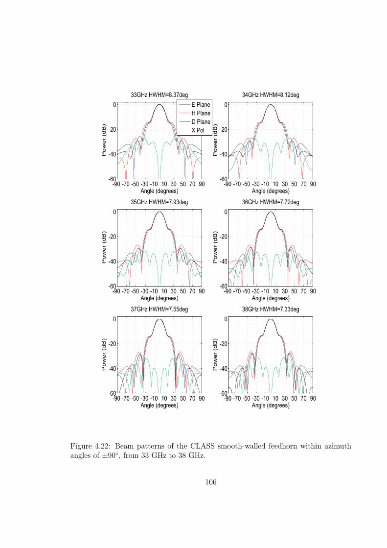
-90 -70 -50 -30 -10 10 30 50 70 90-60
-40
-20
0
Angle (degrees)
Po
we
r (d
B)
33GHz HWHM=8.37deg
E PlaneH PlaneD PlaneX Pol
-90 -70 -50 -30 -10 10 30 50 70 90-60
-40
-20
0
Angle (degrees)
Po
we
r (d
B)
34GHz HWHM=8.12deg
-90 -70 -50 -30 -10 10 30 50 70 90-60
-40
-20
0
Angle (degrees)
Po
we
r (d
B)
35GHz HWHM=7.93deg
-90 -70 -50 -30 -10 10 30 50 70 90-60
-40
-20
0
Angle (degrees)
Po
we
r (d
B)
36GHz HWHM=7.72deg
-90 -70 -50 -30 -10 10 30 50 70 90-60
-40
-20
0
Angle (degrees)
Po
we
r (d
B)
37GHz HWHM=7.55deg
-90 -70 -50 -30 -10 10 30 50 70 90-60
-40
-20
0
Angle (degrees)
Po
we
r (d
B)
38GHz HWHM=7.33deg
Figure 4.22: Beam patterns of the CLASS smooth-walled feedhorn within azimuthangles of ±90, from 33 GHz to 38 GHz.
106
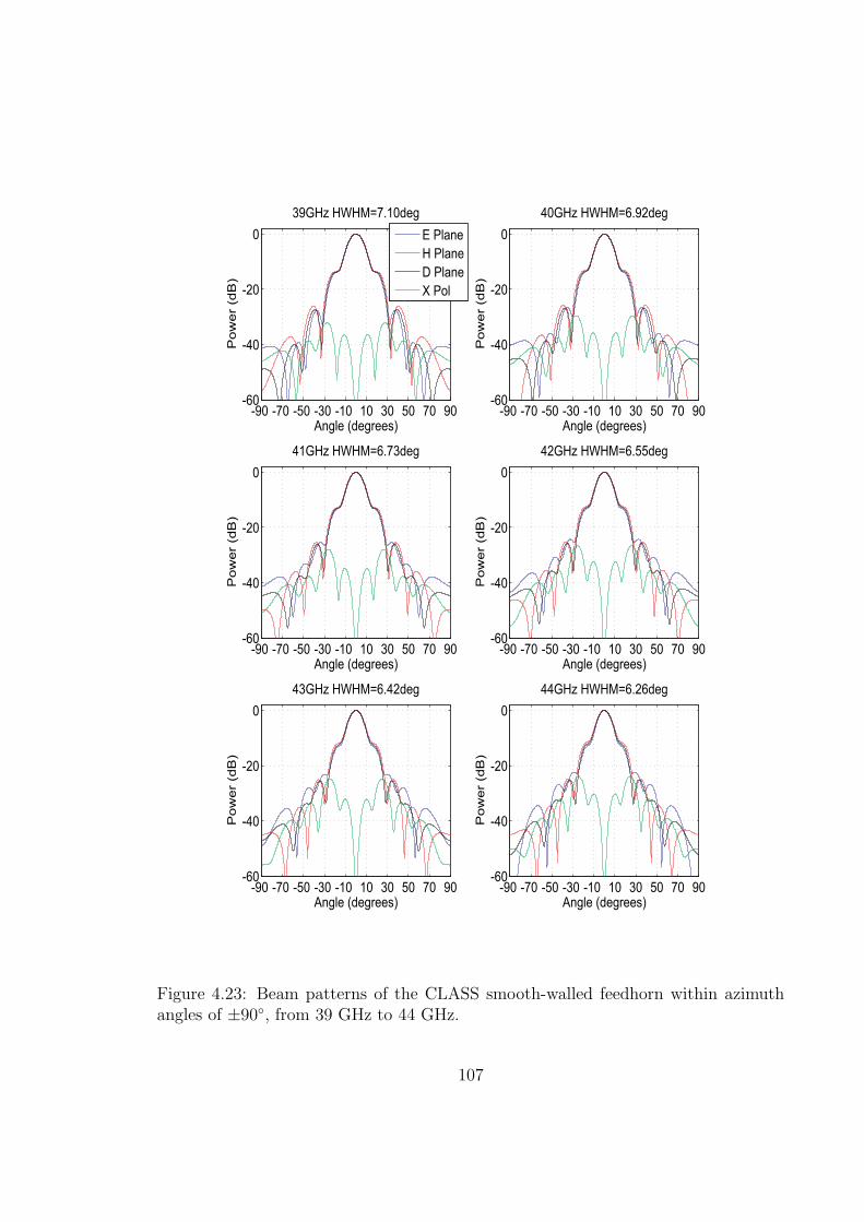
-90 -70 -50 -30 -10 10 30 50 70 90-60
-40
-20
0
Angle (degrees)
Pow
er (
dB)
39GHz HWHM=7.10deg
E PlaneH PlaneD PlaneX Pol
-90 -70 -50 -30 -10 10 30 50 70 90-60
-40
-20
0
Angle (degrees)
Pow
er (
dB)
40GHz HWHM=6.92deg
-90 -70 -50 -30 -10 10 30 50 70 90-60
-40
-20
0
Angle (degrees)
Pow
er (
dB)
41GHz HWHM=6.73deg
-90 -70 -50 -30 -10 10 30 50 70 90-60
-40
-20
0
Angle (degrees)
Pow
er (
dB)
42GHz HWHM=6.55deg
-90 -70 -50 -30 -10 10 30 50 70 90-60
-40
-20
0
Angle (degrees)
Pow
er (
dB)
43GHz HWHM=6.42deg
-90 -70 -50 -30 -10 10 30 50 70 90-60
-40
-20
0
Angle (degrees)
Pow
er (
dB)
44GHz HWHM=6.26deg
Figure 4.23: Beam patterns of the CLASS smooth-walled feedhorn within azimuthangles of ±90, from 39 GHz to 44 GHz.
107
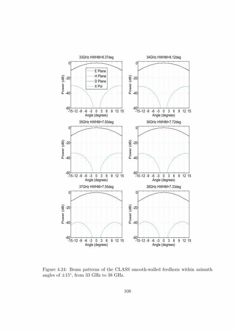
-15 -12 -9 -6 -3 0 3 6 9 12 15-60
-40
-20
0
Angle (degrees)
Po
we
r (d
B)
33GHz HWHM=8.37deg
E PlaneH PlaneD PlaneX Pol
-15 -12 -9 -6 -3 0 3 6 9 12 15-60
-40
-20
0
Angle (degrees)
Po
we
r (d
B)
34GHz HWHM=8.12deg
-15 -12 -9 -6 -3 0 3 6 9 12 15-60
-40
-20
0
Angle (degrees)
Po
we
r (d
B)
35GHz HWHM=7.93deg
-15 -12 -9 -6 -3 0 3 6 9 12 15-60
-40
-20
0
Angle (degrees)
Po
we
r (d
B)
36GHz HWHM=7.72deg
-15 -12 -9 -6 -3 0 3 6 9 12 15-60
-40
-20
0
Angle (degrees)
Po
we
r (d
B)
37GHz HWHM=7.55deg
-15 -12 -9 -6 -3 0 3 6 9 12 15-60
-40
-20
0
Angle (degrees)
Po
we
r (d
B)
38GHz HWHM=7.33deg
Figure 4.24: Beam patterns of the CLASS smooth-walled feedhorn within azimuthangles of ±15, from 33 GHz to 38 GHz.
108
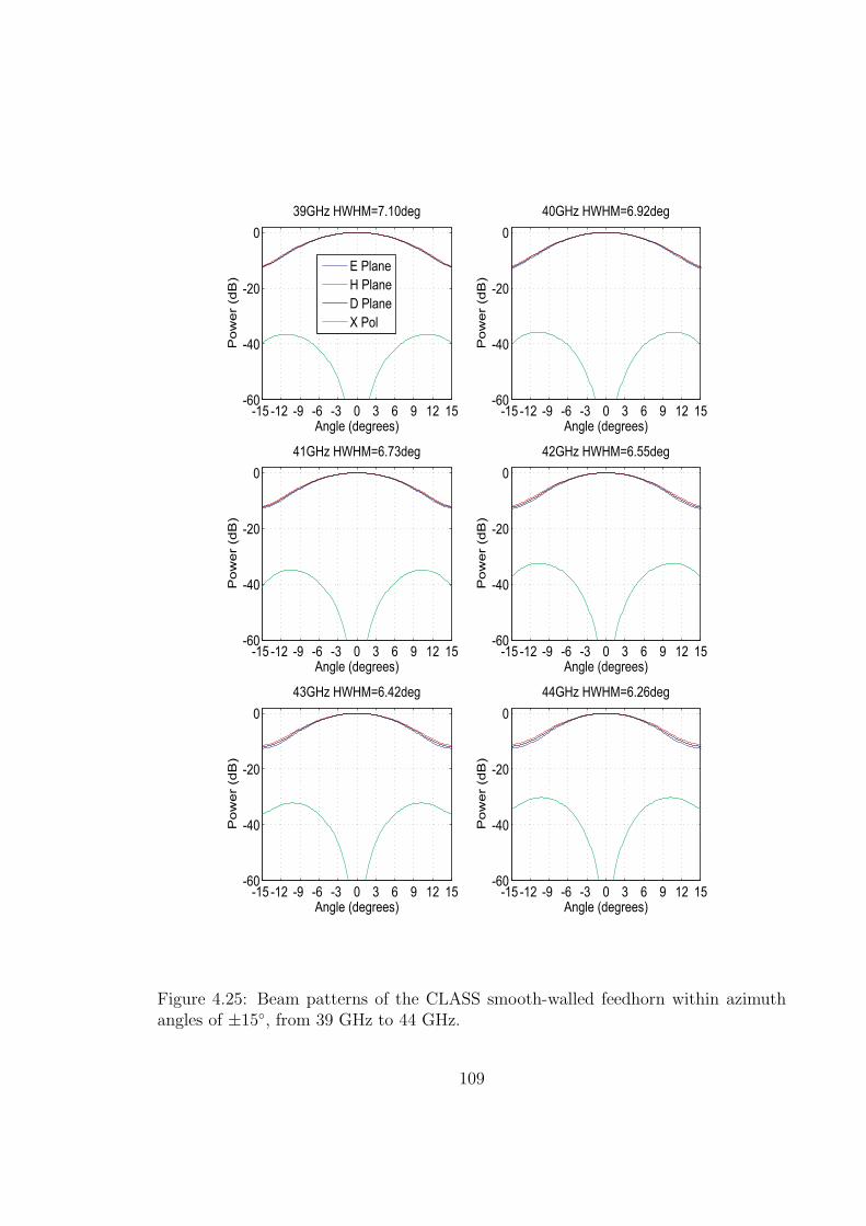
-15 -12 -9 -6 -3 0 3 6 9 12 15-60
-40
-20
0
Angle (degrees)
Pow
er
(dB
)
39GHz HWHM=7.10deg
E PlaneH PlaneD PlaneX Pol
-15 -12 -9 -6 -3 0 3 6 9 12 15-60
-40
-20
0
Angle (degrees)
Pow
er
(dB
)
40GHz HWHM=6.92deg
-15 -12 -9 -6 -3 0 3 6 9 12 15-60
-40
-20
0
Angle (degrees)
Pow
er
(dB
)
41GHz HWHM=6.73deg
-15 -12 -9 -6 -3 0 3 6 9 12 15-60
-40
-20
0
Angle (degrees)
Pow
er
(dB
)
42GHz HWHM=6.55deg
-15 -12 -9 -6 -3 0 3 6 9 12 15-60
-40
-20
0
Angle (degrees)
Pow
er
(dB
)
43GHz HWHM=6.42deg
-15 -12 -9 -6 -3 0 3 6 9 12 15-60
-40
-20
0
Angle (degrees)
Pow
er
(dB
)
44GHz HWHM=6.26deg
Figure 4.25: Beam patterns of the CLASS smooth-walled feedhorn within azimuthangles of ±15, from 39 GHz to 44 GHz.
109
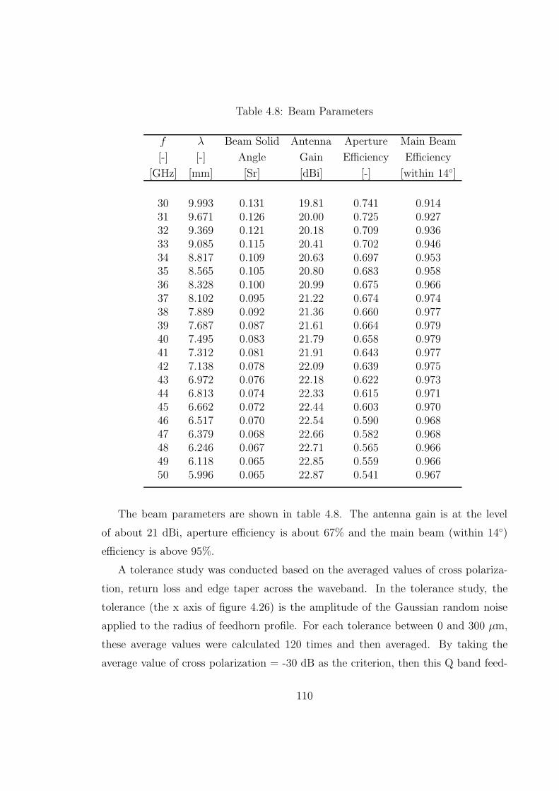
Table 4.8: Beam Parameters
f λ Beam Solid Antenna Aperture Main Beam
[-] [-] Angle Gain Efficiency Efficiency
[GHz] [mm] [Sr] [dBi] [-] [within 14]
30 9.993 0.131 19.81 0.741 0.91431 9.671 0.126 20.00 0.725 0.92732 9.369 0.121 20.18 0.709 0.93633 9.085 0.115 20.41 0.702 0.94634 8.817 0.109 20.63 0.697 0.95335 8.565 0.105 20.80 0.683 0.95836 8.328 0.100 20.99 0.675 0.96637 8.102 0.095 21.22 0.674 0.97438 7.889 0.092 21.36 0.660 0.97739 7.687 0.087 21.61 0.664 0.97940 7.495 0.083 21.79 0.658 0.97941 7.312 0.081 21.91 0.643 0.97742 7.138 0.078 22.09 0.639 0.97543 6.972 0.076 22.18 0.622 0.97344 6.813 0.074 22.33 0.615 0.97145 6.662 0.072 22.44 0.603 0.97046 6.517 0.070 22.54 0.590 0.96847 6.379 0.068 22.66 0.582 0.96848 6.246 0.067 22.71 0.565 0.96649 6.118 0.065 22.85 0.559 0.96650 5.996 0.065 22.87 0.541 0.967
The beam parameters are shown in table 4.8. The antenna gain is at the level
of about 21 dBi, aperture efficiency is about 67% and the main beam (within 14)
efficiency is above 95%.
A tolerance study was conducted based on the averaged values of cross polariza-
tion, return loss and edge taper across the waveband. In the tolerance study, the
tolerance (the x axis of figure 4.26) is the amplitude of the Gaussian random noise
applied to the radius of feedhorn profile. For each tolerance between 0 and 300 µm,
these average values were calculated 120 times and then averaged. By taking the
average value of cross polarization = -30 dB as the criterion, then this Q band feed-
110
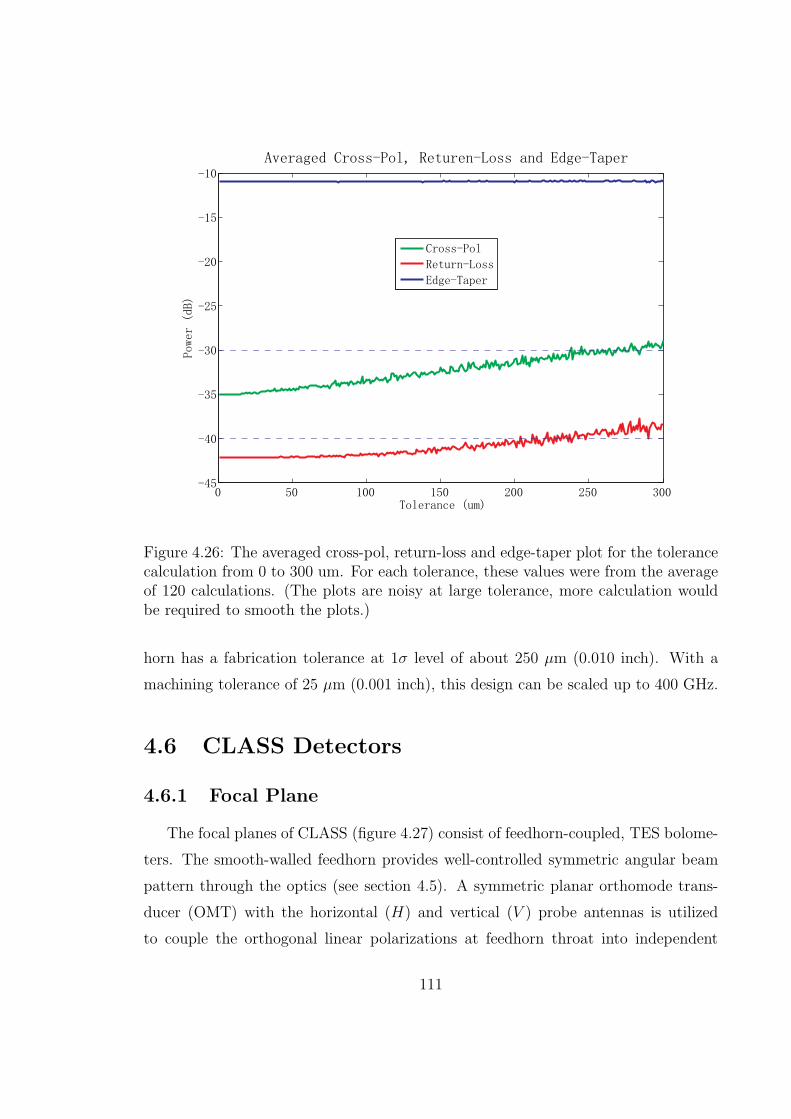
Figure 4.26: The averaged cross-pol, return-loss and edge-taper plot for the tolerancecalculation from 0 to 300 um. For each tolerance, these values were from the averageof 120 calculations. (The plots are noisy at large tolerance, more calculation wouldbe required to smooth the plots.)
horn has a fabrication tolerance at 1σ level of about 250 µm (0.010 inch). With a
machining tolerance of 25 µm (0.001 inch), this design can be scaled up to 400 GHz.
4.6 CLASS Detectors
4.6.1 Focal Plane
The focal planes of CLASS (figure 4.27) consist of feedhorn-coupled, TES bolome-
ters. The smooth-walled feedhorn provides well-controlled symmetric angular beam
pattern through the optics (see section 4.5). A symmetric planar orthomode trans-
ducer (OMT) with the horizontal (H) and vertical (V ) probe antennas is utilized
to couple the orthogonal linear polarizations at feedhorn throat into independent
111
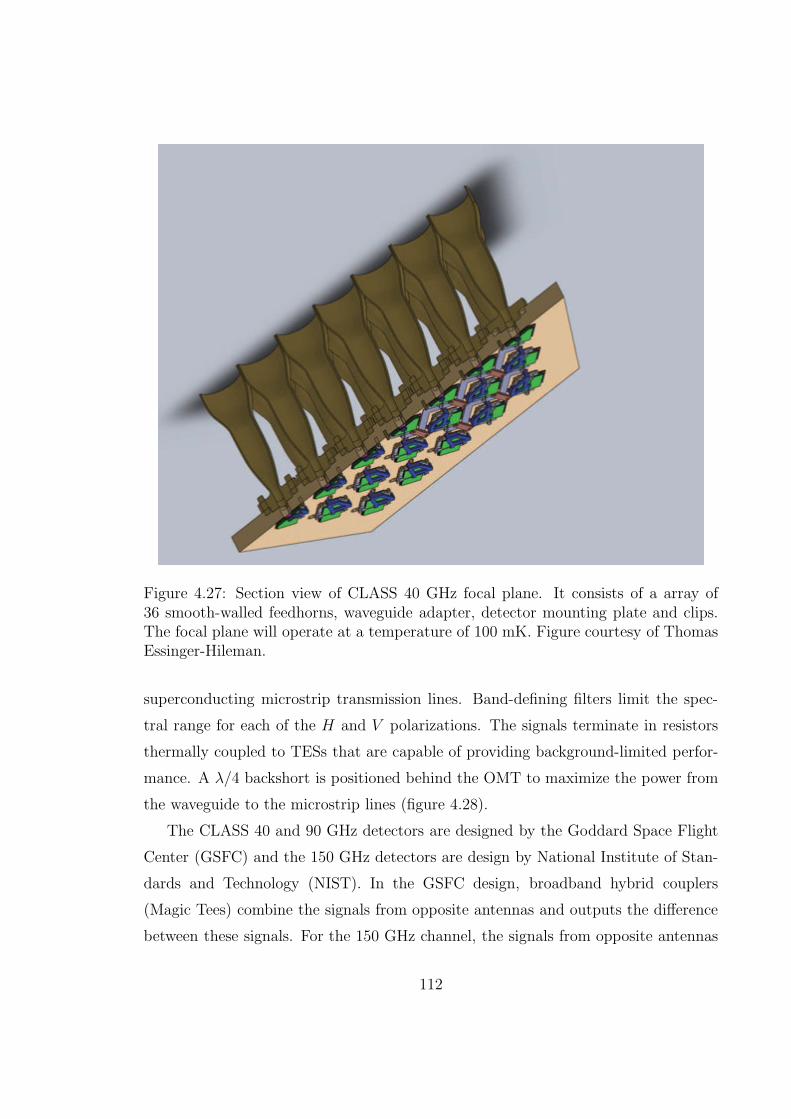
Figure 4.27: Section view of CLASS 40 GHz focal plane. It consists of a array of36 smooth-walled feedhorns, waveguide adapter, detector mounting plate and clips.The focal plane will operate at a temperature of 100 mK. Figure courtesy of ThomasEssinger-Hileman.
superconducting microstrip transmission lines. Band-defining filters limit the spec-
tral range for each of the H and V polarizations. The signals terminate in resistors
thermally coupled to TESs that are capable of providing background-limited perfor-
mance. A λ/4 backshort is positioned behind the OMT to maximize the power from
the waveguide to the microstrip lines (figure 4.28).
The CLASS 40 and 90 GHz detectors are designed by the Goddard Space Flight
Center (GSFC) and the 150 GHz detectors are design by National Institute of Stan-
dards and Technology (NIST). In the GSFC design, broadband hybrid couplers
(Magic Tees) combine the signals from opposite antennas and outputs the difference
between these signals. For the 150 GHz channel, the signals from opposite antennas
112
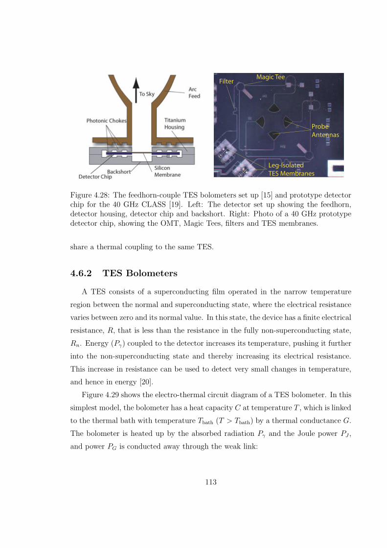
Figure 4.28: The feedhorn-couple TES bolometers set up [15] and prototype detectorchip for the 40 GHz CLASS [19]. Left: The detector set up showing the feedhorn,detector housing, detector chip and backshort. Right: Photo of a 40 GHz prototypedetector chip, showing the OMT, Magic Tees, filters and TES membranes.
share a thermal coupling to the same TES.
4.6.2 TES Bolometers
A TES consists of a superconducting film operated in the narrow temperature
region between the normal and superconducting state, where the electrical resistance
varies between zero and its normal value. In this state, the device has a finite electrical
resistance, R, that is less than the resistance in the fully non-superconducting state,
Rn. Energy (Pγ) coupled to the detector increases its temperature, pushing it further
into the non-superconducting state and thereby increasing its electrical resistance.
This increase in resistance can be used to detect very small changes in temperature,
and hence in energy [20].
Figure 4.29 shows the electro-thermal circuit diagram of a TES bolometer. In this
simplest model, the bolometer has a heat capacity C at temperature T , which is linked
to the thermal bath with temperature Tbath (T > Tbath) by a thermal conductance G.
The bolometer is heated up by the absorbed radiation Pγ and the Joule power PJ ,
and power PG is conducted away through the weak link:
113
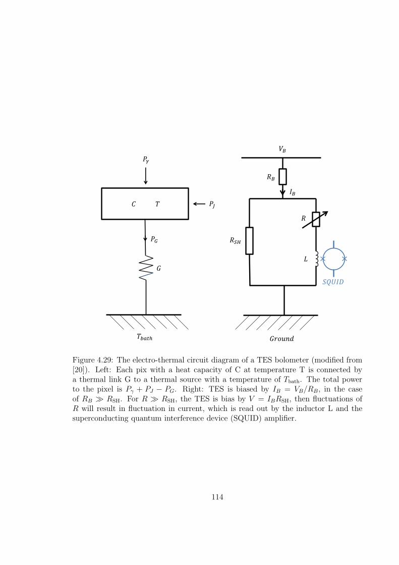
Figure 4.29: The electro-thermal circuit diagram of a TES bolometer (modified from[20]). Left: Each pix with a heat capacity of C at temperature T is connected bya thermal link G to a thermal source with a temperature of Tbath. The total powerto the pixel is Pγ + PJ − PG. Right: TES is biased by IB = VB/RB, in the caseof RB ≫ RSH. For R ≫ RSH, the TES is bias by V = IBRSH, then fluctuations ofR will result in fluctuation in current, which is read out by the inductor L and thesuperconducting quantum interference device (SQUID) amplifier.
114
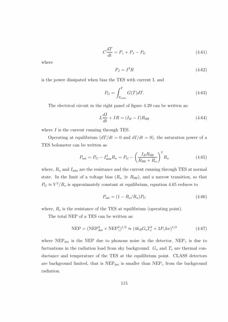
CdT
dt= Pγ + PJ − PG (4.61)
where
PJ = I2R (4.62)
is the power dissipated when bias the TES with current I, and
PG =
∫ T
Tbath
G(T )dT. (4.63)
The electrical circuit in the right panel of figure 4.29 can be written as:
LdI
dt+ IR = (IB − I)RSH (4.64)
where I is the current running through TES.
Operating at equilibrium (dT/dt = 0 and dI/dt = 0), the saturation power of a
TES bolometer can be written as
Psat = PG − I2minRn = PG −(
IBRSH
RSH +Rn
)2
Rn (4.65)
where, Rn and Imin are the resistance and the current running through TES at normal
state. In the limit of a voltage bias (Rn ≫ RSH), and a narrow transition, so that
PG ≈ V 2/Ro is approximately constant at equilibrium, equation 4.65 reduces to
Psat = (1−Ro/Rn)PG (4.66)
where, Ro is the resistance of the TES at equilibrium (operating point).
The total NEP of a TES can be written as:
NEP = (NEP2det +NEP2
γ)1/2 ≈ (4kBGoT
2o + 2Pγhν)
1/2 (4.67)
where NEPdet is the NEP due to phonons noise in the detector, NEPγ is due to
fuctuations in the radiation load from sky background. Go and To are thermal con-
ductance and temperature of the TES at the equilibrium point. CLASS detectors
are background limited, that is NEPdet is smaller than NEPγ from the background
radiation.
115
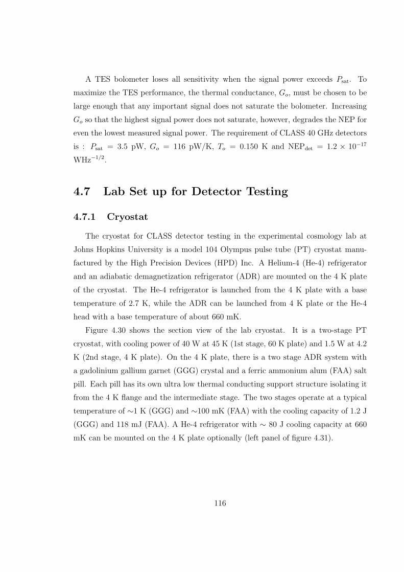
A TES bolometer loses all sensitivity when the signal power exceeds Psat. To
maximize the TES performance, the thermal conductance, Go, must be chosen to be
large enough that any important signal does not saturate the bolometer. Increasing
Go so that the highest signal power does not saturate, however, degrades the NEP for
even the lowest measured signal power. The requirement of CLASS 40 GHz detectors
is : Psat = 3.5 pW, Go = 116 pW/K, To = 0.150 K and NEPdet = 1.2 × 10⁻¹⁷
WHz−1/2.
4.7 Lab Set up for Detector Testing
4.7.1 Cryostat
The cryostat for CLASS detector testing in the experimental cosmology lab at
Johns Hopkins University is a model 104 Olympus pulse tube (PT) cryostat manu-
factured by the High Precision Devices (HPD) Inc. A Helium-4 (He-4) refrigerator
and an adiabatic demagnetization refrigerator (ADR) are mounted on the 4 K plate
of the cryostat. The He-4 refrigerator is launched from the 4 K plate with a base
temperature of 2.7 K, while the ADR can be launched from 4 K plate or the He-4
head with a base temperature of about 660 mK.
Figure 4.30 shows the section view of the lab cryostat. It is a two-stage PT
cryostat, with cooling power of 40 W at 45 K (1st stage, 60 K plate) and 1.5 W at 4.2
K (2nd stage, 4 K plate). On the 4 K plate, there is a two stage ADR system with
a gadolinium gallium garnet (GGG) crystal and a ferric ammonium alum (FAA) salt
pill. Each pill has its own ultra low thermal conducting support structure isolating it
from the 4 K flange and the intermediate stage. The two stages operate at a typical
temperature of ∼1 K (GGG) and ∼100 mK (FAA) with the cooling capacity of 1.2 J
(GGG) and 118 mJ (FAA). A He-4 refrigerator with ∼ 80 J cooling capacity at 660
mK can be mounted on the 4 K plate optionally (left panel of figure 4.31).
116
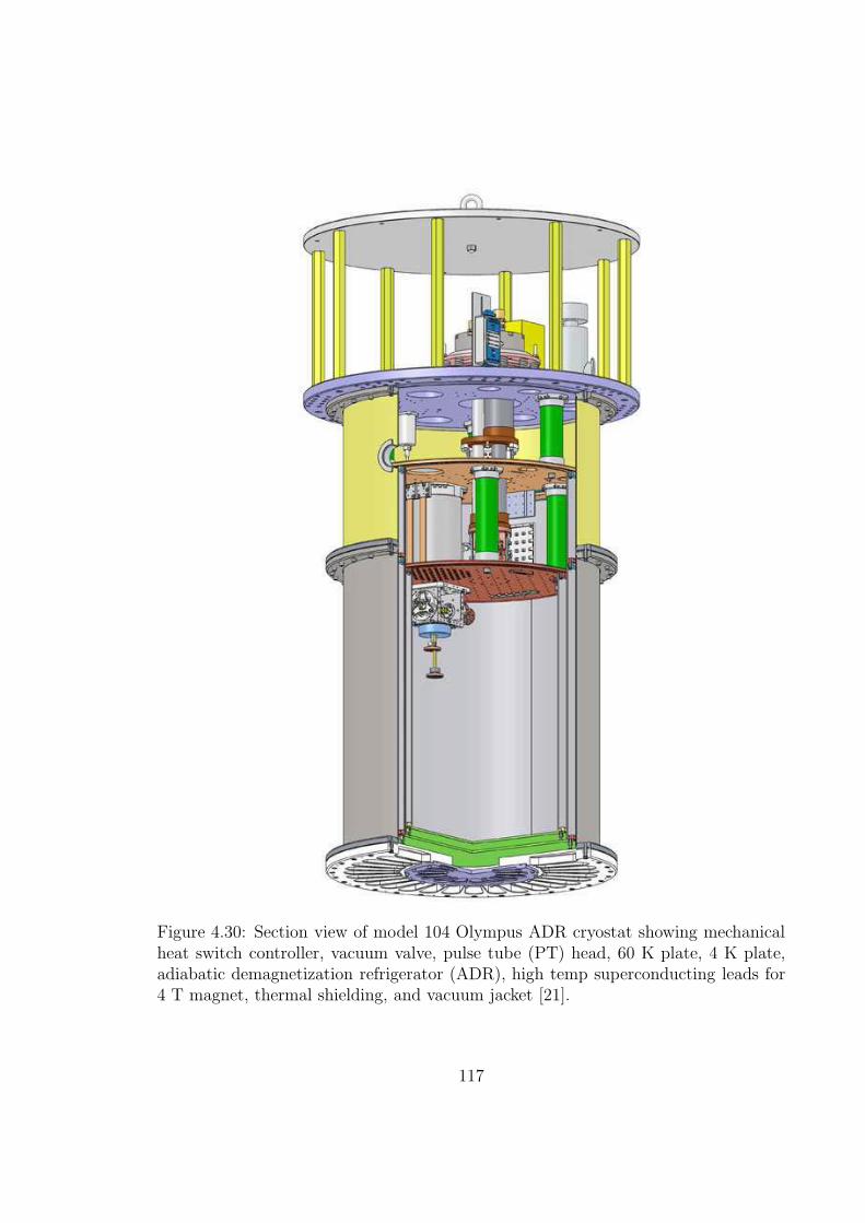
Figure 4.30: Section view of model 104 Olympus ADR cryostat showing mechanicalheat switch controller, vacuum valve, pulse tube (PT) head, 60 K plate, 4 K plate,adiabatic demagnetization refrigerator (ADR), high temp superconducting leads for4 T magnet, thermal shielding, and vacuum jacket [21].
117
4.7.2 Thermometry
The thermometry of the lab cryostat includes a general thermometer readout
system and an ADR Proportional-Integral-Derivative (PID) control system. The
general sensor readout system consists of a Stanford Research Systems (SRS) SIM900
mainframe with GPIB port, two SIM925 octal four-wire multiplexers (MUXs), a
SIM922 diode temperature monitor and a SIM921 AC resistance bridge. MUX 1
is for reading out silicon diodes and MUX 2 is for reading out ruthenium oxide
(RuOx) and other resistance temperature detectors (RTDs). The ADR PID control
system includes a Lakeshore model 370 AC resistance bridge, a calibrated GR-50-AA
germanium resistance temperature (GRT) sensor (mounted inside the cryostat) and
two Keithley model 2440 5 A sourcemeters. The above devices communicate with
a cryostat computer through a National Instruments (NI) model GPIB-ENET/100
GPIB to Ethernet adapter (right panel of figure 4.31). The mechanical heat switch
of the ADR is controlled via a NI USB-6009 Data Acquisition (DAQ) device.
The thermometry is control by LabVIEW programs (see appendix F for details).
For general thermometer readout, the program loops over the two octal MUXs to
produce real time plots. In the mean time, it also displays and saves all data with
time stamps. The readout process is in series. Due to the delay in each readout
caused by the response time of the diode monitor and the AC resistance bridge, it
take about 120 seconds to finish a single loop for reading out all channels of two
MUXs. To regulate the ADR temperature, the PID program reads the temperature
from the GRT sensor through the Lakeshore AC resistance bridge, calculates the
output to the Keithley current source by the PID algorithm, and controls the current
in the ADR magnet. This program also produces real time plots of the temperature
and error between the temperature and the set point. The temperature and the
magnet current are saved with time stamps in a file.
4.7.3 Cryostat Performance
Figure 4.32 shows the cool down curves of the cryostat from warm temperature
(∼ 300 K) to cool temperature (equilibrium temperature). It takes about 24 hours
118
Figure 4.31: Left: The ADR and the He-4 refrigerator mounted on the 4 K plate of theHPD cryostat in the experimental cosmology lab at Johns Hopkins University. Photocourtesy of David Larson. Right: the rack-mounted devices for cryostat thermometry.From top to bottom, they are, a SRS SIM900 mainframe with 2 MUXs, a diodemoniter and an AC bridge, a front panel, a NI GPIB to Ethernet adapter, a Lakeshore370 AC resistance bridge and two Keithley 2440 current sources.
for the cryostat to cool down to the state with stable temperature readouts. The
typical values of the thermometers are listed in table 4.9. The 60 K plate can reach
the temperature of 50.0 K and the 4 K plate can get as lower as 2.7 K.
Launching from the 4 K plate with a 2.7 K base temperature, the ADR can last
for about 210 hour at 100 mK with no load (FAA pill). Thus, the intrinsic thermal
load of the FAA pill is around 0.15 µW. Figure 4.33 shows the cooling curves (the
magnet current versus time) of the ADR with the loads of from 2.0 to 10.0 µW.
Based on these curves, the FAA pill of the ADR have higher cooling capacities at
lower loads. With a 2 µW load, the cooling capacity is about 130 mJ, which is close
to the theoretical number of 118 mJ. While with a 10 µW load, the capacity drops
to about 50 mJ.
4.7.4 Detector Readout
The signal from the TES bolometers is read out by two stages of the supercon-
ducting quantum interference device (SQUID) amplifier. The output of the SQUID
amplifier is a voltage that is approximately a sinusoidal function of the magnetic flux
119
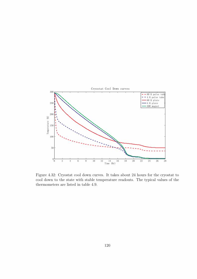
Figure 4.32: Cryostat cool down curves. It takes about 24 hours for the cryostat tocool down to the state with stable temperature readouts. The typical values of thethermometers are listed in table 4.9.
120
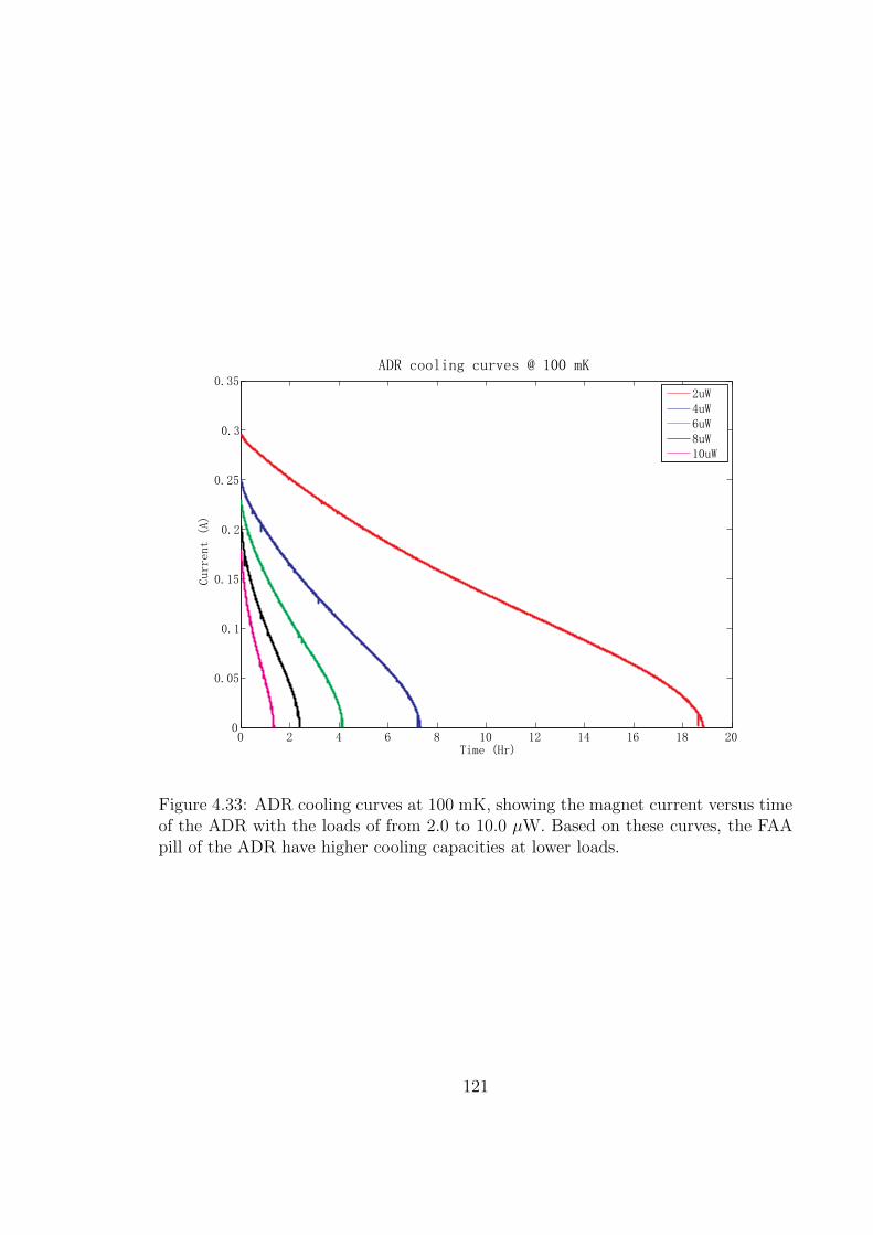
Figure 4.33: ADR cooling curves at 100 mK, showing the magnet current versus timeof the ADR with the loads of from 2.0 to 10.0 µW. Based on these curves, the FAApill of the ADR have higher cooling capacities at lower loads.
121
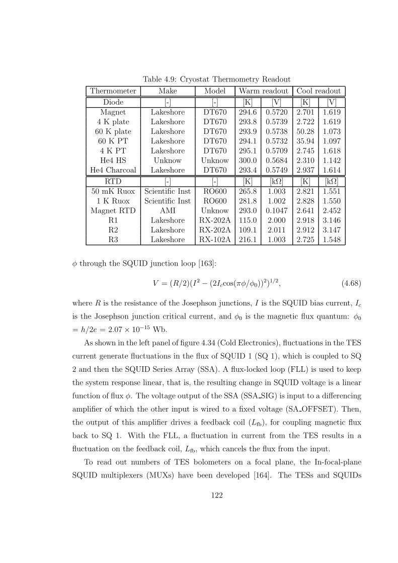
Table 4.9: Cryostat Thermometry Readout
Thermometer Make Model Warm readout Cool readout
Diode [-] [-] [K] [V] [K] [V]Magnet Lakeshore DT670 294.6 0.5720 2.701 1.6194 K plate Lakeshore DT670 293.8 0.5739 2.722 1.61960 K plate Lakeshore DT670 293.9 0.5738 50.28 1.07360 K PT Lakeshore DT670 294.1 0.5732 35.94 1.0974 K PT Lakeshore DT670 295.1 0.5709 2.745 1.618He4 HS Unknow Unknow 300.0 0.5684 2.310 1.142
He4 Charcoal Lakeshore DT670 293.4 0.5749 2.937 1.614
RTD [-] [-] [K] [kΩ] [K] [kΩ]50 mK Ruox Scientific Inst RO600 265.8 1.003 2.821 1.5511 K Ruox Scientific Inst RO600 281.8 1.002 2.828 1.550
Magnet RTD AMI Unknow 293.0 0.1047 2.641 2.452R1 Lakeshore RX-202A 115.0 2.000 2.918 3.146R2 Lakeshore RX-202A 109.1 2.011 2.912 3.147R3 Lakeshore RX-102A 216.1 1.003 2.725 1.548
φ through the SQUID junction loop [163]:
V = (R/2)(I2 − (2Iccos(πφ/φ0))2)1/2, (4.68)
where R is the resistance of the Josephson junctions, I is the SQUID bias current, Ic
is the Josephson junction critical current, and φ0 is the magnetic flux quantum: φ0
= h/2e = 2.07× 10⁻¹⁵ Wb.
As shown in the left panel of figure 4.34 (Cold Electronics), fluctuations in the TES
current generate fluctuations in the flux of SQUID 1 (SQ 1), which is coupled to SQ
2 and then the SQUID Series Array (SSA). A flux-locked loop (FLL) is used to keep
the system response linear, that is, the resulting change in SQUID voltage is a linear
function of flux φ. The voltage output of the SSA (SSA SIG) is input to a differencing
amplifier of which the other input is wired to a fixed voltage (SA OFFSET). Then,
the output of this amplifier drives a feedback coil (Lfb), for coupling magnetic flux
back to SQ 1. With the FLL, a fluctuation in current from the TES results in a
fluctuation on the feedback coil, Lfb, which cancels the flux from the input.
To read out numbers of TES bolometers on a focal plane, the In-focal-plane
SQUID multiplexers (MUXs) have been developed [164]. The TESs and SQUIDs
122
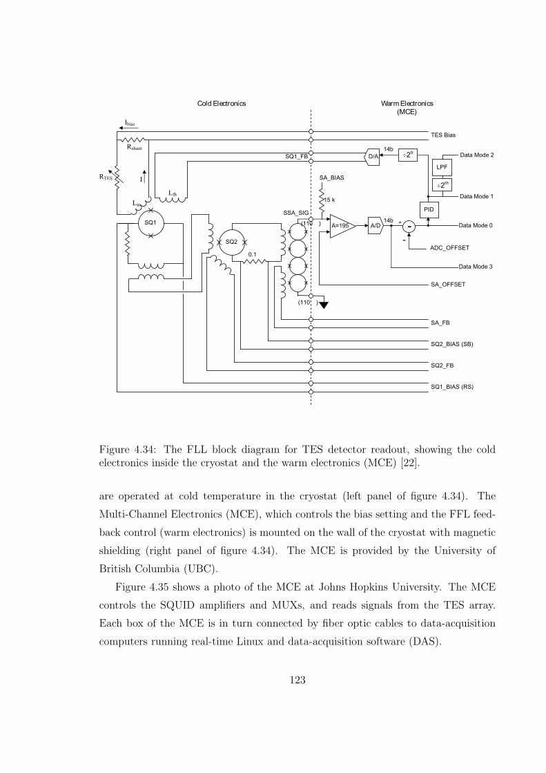
SQ1
SQ2
SA_BIAS
SA_OFFSET
A/D
D/A
PID
SA_FB
SQ2_BIAS (SB)
SQ2_FB
SQ1_BIAS (RS)
0.1
15 k
TES Bias
ADC_OFFSET
SQ1_FB
(110 )
(110 )
-
14b
14b
SSA_SIG
+
-
LPF
Cold Electronics Warm Electronics (MCE)
A=195
÷2n
÷2m
Ibias
I
Lin
Lfb
Rshunt
RTES
Data Mode 2
Data Mode 0
Data Mode 1
Data Mode 3
Figure 4.34: The FLL block diagram for TES detector readout, showing the coldelectronics inside the cryostat and the warm electronics (MCE) [22].
are operated at cold temperature in the cryostat (left panel of figure 4.34). The
Multi-Channel Electronics (MCE), which controls the bias setting and the FFL feed-
back control (warm electronics) is mounted on the wall of the cryostat with magnetic
shielding (right panel of figure 4.34). The MCE is provided by the University of
British Columbia (UBC).
Figure 4.35 shows a photo of the MCE at Johns Hopkins University. The MCE
controls the SQUID amplifiers and MUXs, and reads signals from the TES array.
Each box of the MCE is in turn connected by fiber optic cables to data-acquisition
computers running real-time Linux and data-acquisition software (DAS).
123
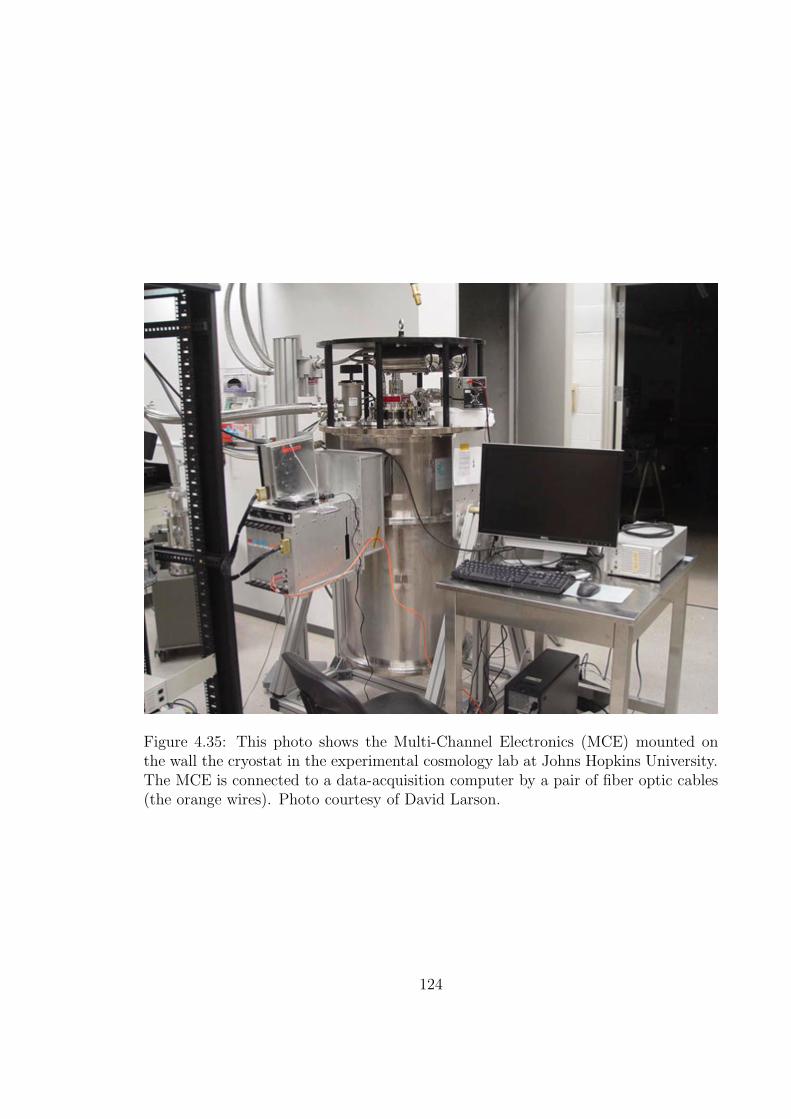
Figure 4.35: This photo shows the Multi-Channel Electronics (MCE) mounted onthe wall the cryostat in the experimental cosmology lab at Johns Hopkins University.The MCE is connected to a data-acquisition computer by a pair of fiber optic cables(the orange wires). Photo courtesy of David Larson.
124
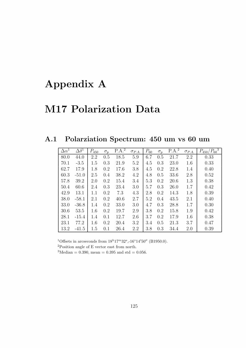
Appendix A
M17 Polarization Data
A.1 Polarziation Spectrum: 450 um vs 60 um
∆α1 ∆δ1 P450 σp P.A.2 σP.A. P60 σp P.A.2 σP.A. P450/P603
80.0 44.0 2.2 0.5 18.5 5.9 6.7 0.5 21.7 2.2 0.3370.1 -3.5 1.5 0.3 21.9 5.2 4.5 0.3 23.0 1.6 0.3362.7 17.9 1.8 0.2 17.6 3.8 4.5 0.2 22.8 1.4 0.4060.3 -51.0 2.5 0.4 38.2 4.2 4.8 0.5 33.6 2.8 0.5257.8 39.2 2.0 0.2 15.4 3.4 5.3 0.2 20.6 1.3 0.3850.4 60.6 2.4 0.3 23.4 3.0 5.7 0.3 26.0 1.7 0.4242.9 13.1 1.1 0.2 7.3 4.3 2.8 0.2 14.3 1.8 0.3938.0 -58.1 2.1 0.2 40.6 2.7 5.2 0.4 43.5 2.1 0.4033.0 -36.8 1.4 0.2 33.0 3.0 4.7 0.3 28.8 1.7 0.3030.6 53.5 1.6 0.2 19.7 2.9 3.8 0.2 15.8 1.9 0.4228.1 -15.4 1.4 0.1 12.7 2.6 3.7 0.2 17.9 1.6 0.3823.1 77.2 1.6 0.2 20.4 3.2 3.4 0.5 21.3 3.7 0.4713.2 -41.5 1.5 0.1 26.4 2.2 3.8 0.3 34.4 2.0 0.39
1Offsets in arcseconds from 18h17m32s,-1614′50′′ (B1950.0).2Position angle of E vector east from north.3Median = 0.390, mean = 0.395 and std = 0.056.
125

Figure A.1: 60 um polarization vectors from Stokes ([23], Yellow) and the 450 umresult from SHARP (smoothed to 22′′ resolution, Red), center at 18h17m32s,-1614′25′′
(B1950.0).
126
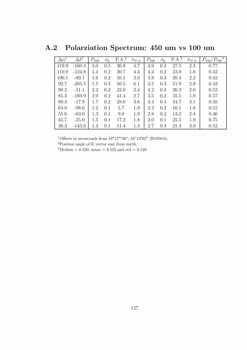
A.2 Polarziation Spectrum: 450 um vs 100 um
∆α1 ∆δ1 P450 σp P.A.2 σP.A. P100 σp P.A.2 σP.A. P450/P1003
119.9 -160.4 3.0 0.5 36.9 4.7 3.9 0.3 27.5 2.3 0.77110.0 -124.8 1.4 0.2 30.7 4.4 4.4 0.2 23.0 1.6 0.32100.1 -89.1 1.6 0.2 16.1 3.0 3.8 0.3 20.4 2.2 0.4292.7 -205.5 1.5 0.3 50.5 6.1 3.5 0.3 51.9 2.9 0.4390.2 -51.1 2.2 0.2 22.0 2.4 4.2 0.3 26.3 2.0 0.5285.3 -169.9 2.0 0.2 41.4 2.7 3.5 0.2 35.5 1.9 0.5780.3 -17.9 1.7 0.2 28.6 3.6 3.4 0.4 34.7 3.1 0.5063.0 -98.6 1.2 0.1 5.7 1.9 2.3 0.2 10.1 1.8 0.5255.6 -63.0 1.3 0.1 9.8 1.9 2.8 0.2 13.2 2.4 0.4645.7 -25.0 1.5 0.1 17.2 1.8 2.0 0.1 25.5 1.9 0.7538.3 -143.8 1.4 0.1 11.4 1.4 2.7 0.3 21.3 3.0 0.52
1Offsets in arcseconds from 18h17m30s,-1613′03′′ (B1950.0).2Position angle of E vector east from north.3Median = 0.520, mean = 0.525 and std = 0.128.
127
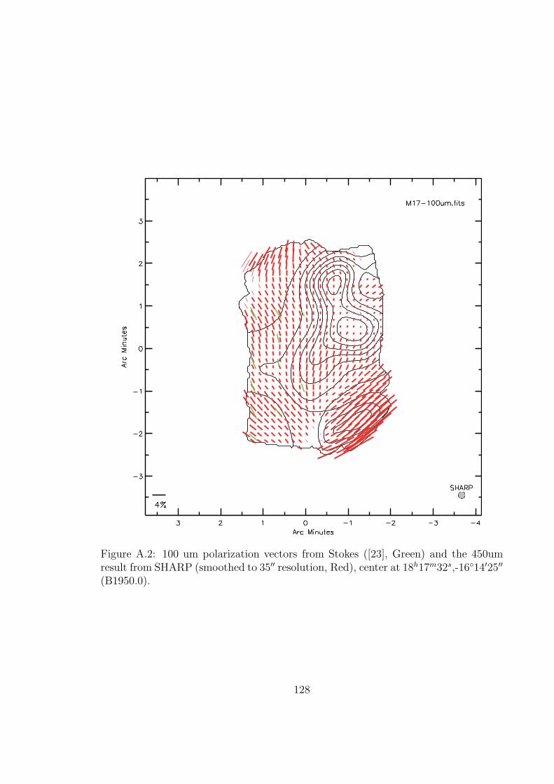
Figure A.2: 100 um polarization vectors from Stokes ([23], Green) and the 450umresult from SHARP (smoothed to 35′′ resolution, Red), center at 18h17m32s,-1614′25′′
(B1950.0).
128
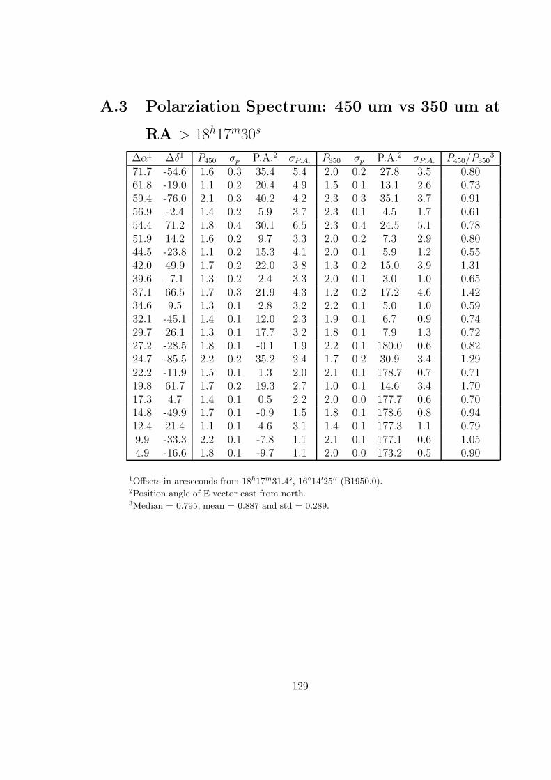
A.3 Polarziation Spectrum: 450 um vs 350 um at
RA > 18h17
m30
s
∆α1 ∆δ1 P450 σp P.A.2 σP.A. P350 σp P.A.2 σP.A. P450/P3503
71.7 -54.6 1.6 0.3 35.4 5.4 2.0 0.2 27.8 3.5 0.8061.8 -19.0 1.1 0.2 20.4 4.9 1.5 0.1 13.1 2.6 0.7359.4 -76.0 2.1 0.3 40.2 4.2 2.3 0.3 35.1 3.7 0.9156.9 -2.4 1.4 0.2 5.9 3.7 2.3 0.1 4.5 1.7 0.6154.4 71.2 1.8 0.4 30.1 6.5 2.3 0.4 24.5 5.1 0.7851.9 14.2 1.6 0.2 9.7 3.3 2.0 0.2 7.3 2.9 0.8044.5 -23.8 1.1 0.2 15.3 4.1 2.0 0.1 5.9 1.2 0.5542.0 49.9 1.7 0.2 22.0 3.8 1.3 0.2 15.0 3.9 1.3139.6 -7.1 1.3 0.2 2.4 3.3 2.0 0.1 3.0 1.0 0.6537.1 66.5 1.7 0.3 21.9 4.3 1.2 0.2 17.2 4.6 1.4234.6 9.5 1.3 0.1 2.8 3.2 2.2 0.1 5.0 1.0 0.5932.1 -45.1 1.4 0.1 12.0 2.3 1.9 0.1 6.7 0.9 0.7429.7 26.1 1.3 0.1 17.7 3.2 1.8 0.1 7.9 1.3 0.7227.2 -28.5 1.8 0.1 -0.1 1.9 2.2 0.1 180.0 0.6 0.8224.7 -85.5 2.2 0.2 35.2 2.4 1.7 0.2 30.9 3.4 1.2922.2 -11.9 1.5 0.1 1.3 2.0 2.1 0.1 178.7 0.7 0.7119.8 61.7 1.7 0.2 19.3 2.7 1.0 0.1 14.6 3.4 1.7017.3 4.7 1.4 0.1 0.5 2.2 2.0 0.0 177.7 0.6 0.7014.8 -49.9 1.7 0.1 -0.9 1.5 1.8 0.1 178.6 0.8 0.9412.4 21.4 1.1 0.1 4.6 3.1 1.4 0.1 177.3 1.1 0.799.9 -33.3 2.2 0.1 -7.8 1.1 2.1 0.1 177.1 0.6 1.054.9 -16.6 1.8 0.1 -9.7 1.1 2.0 0.0 173.2 0.5 0.90
1Offsets in arcseconds from 18h17m31.4s,-1614′25′′ (B1950.0).2Position angle of E vector east from north.3Median = 0.795, mean = 0.887 and std = 0.289.
129
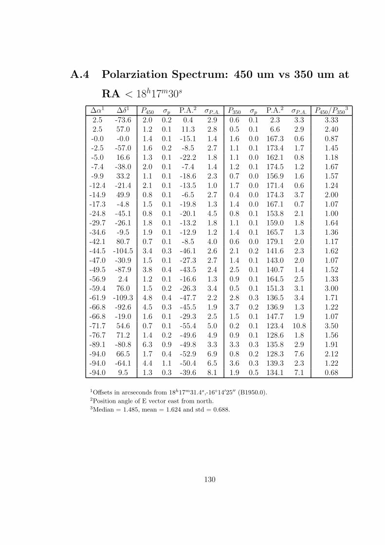
A.4 Polarziation Spectrum: 450 um vs 350 um at
RA < 18h17
m30
s
∆α1 ∆δ1 P450 σp P.A.2 σP.A. P350 σp P.A.2 σP.A. P450/P3503
2.5 -73.6 2.0 0.2 0.4 2.9 0.6 0.1 2.3 3.3 3.332.5 57.0 1.2 0.1 11.3 2.8 0.5 0.1 6.6 2.9 2.40-0.0 -0.0 1.4 0.1 -15.1 1.4 1.6 0.0 167.3 0.6 0.87-2.5 -57.0 1.6 0.2 -8.5 2.7 1.1 0.1 173.4 1.7 1.45-5.0 16.6 1.3 0.1 -22.2 1.8 1.1 0.0 162.1 0.8 1.18-7.4 -38.0 2.0 0.1 -7.4 1.4 1.2 0.1 174.5 1.2 1.67-9.9 33.2 1.1 0.1 -18.6 2.3 0.7 0.0 156.9 1.6 1.57-12.4 -21.4 2.1 0.1 -13.5 1.0 1.7 0.0 171.4 0.6 1.24-14.9 49.9 0.8 0.1 -6.5 2.7 0.4 0.0 174.3 3.7 2.00-17.3 -4.8 1.5 0.1 -19.8 1.3 1.4 0.0 167.1 0.7 1.07-24.8 -45.1 0.8 0.1 -20.1 4.5 0.8 0.1 153.8 2.1 1.00-29.7 -26.1 1.8 0.1 -13.2 1.8 1.1 0.1 159.0 1.8 1.64-34.6 -9.5 1.9 0.1 -12.9 1.2 1.4 0.1 165.7 1.3 1.36-42.1 80.7 0.7 0.1 -8.5 4.0 0.6 0.0 179.1 2.0 1.17-44.5 -104.5 3.4 0.3 -46.1 2.6 2.1 0.2 141.6 2.3 1.62-47.0 -30.9 1.5 0.1 -27.3 2.7 1.4 0.1 143.0 2.0 1.07-49.5 -87.9 3.8 0.4 -43.5 2.4 2.5 0.1 140.7 1.4 1.52-56.9 2.4 1.2 0.1 -16.6 1.3 0.9 0.1 164.5 2.5 1.33-59.4 76.0 1.5 0.2 -26.3 3.4 0.5 0.1 151.3 3.1 3.00-61.9 -109.3 4.8 0.4 -47.7 2.2 2.8 0.3 136.5 3.4 1.71-66.8 -92.6 4.5 0.3 -45.5 1.9 3.7 0.2 136.9 1.3 1.22-66.8 -19.0 1.6 0.1 -29.3 2.5 1.5 0.1 147.7 1.9 1.07-71.7 54.6 0.7 0.1 -55.4 5.0 0.2 0.1 123.4 10.8 3.50-76.7 71.2 1.4 0.2 -49.6 4.9 0.9 0.1 128.6 1.8 1.56-89.1 -80.8 6.3 0.9 -49.8 3.3 3.3 0.3 135.8 2.9 1.91-94.0 66.5 1.7 0.4 -52.9 6.9 0.8 0.2 128.3 7.6 2.12-94.0 -64.1 4.4 1.1 -50.4 6.5 3.6 0.3 139.3 2.3 1.22-94.0 9.5 1.3 0.3 -39.6 8.1 1.9 0.5 134.1 7.1 0.68
1Offsets in arcseconds from 18h17m31.4s,-1614′25′′ (B1950.0).2Position angle of E vector east from north.3Median = 1.485, mean = 1.624 and std = 0.688.
130
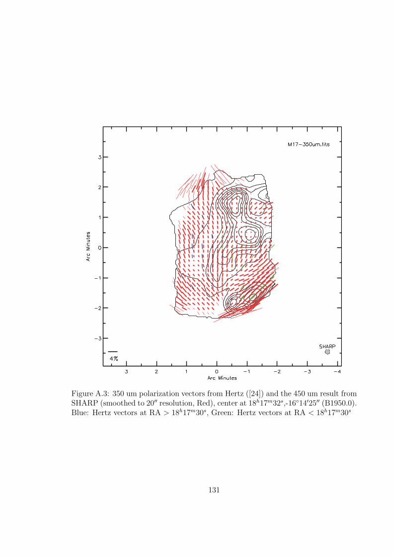
Figure A.3: 350 um polarization vectors from Hertz ([24]) and the 450 um result fromSHARP (smoothed to 20′′ resolution, Red), center at 18h17m32s,-1614′25′′ (B1950.0).Blue: Hertz vectors at RA > 18h17m30s, Green: Hertz vectors at RA < 18h17m30s
131

A.5 Polarization Vectors
∆α1 ∆δ1 P σp P.A.2 σP.A. ∆α ∆δ P σp P.A. σP.A.
70.2 -114.0 5.8 2.5 51.7 12.1 -18.9 -19.0 2.5 0.2 -18.4 2.7
70.2 -95.0 5.0 2.1 36.4 11.9 -18.9 -9.5 1.6 0.2 -23.6 3.9
70.1 -57.0 3.1 1.5 32.0 12.8 -18.9 -0.0 1.4 0.3 -34.6 5.9
70.1 -38.0 3.4 1.7 5.6 13.7 -18.9 9.5 1.4 0.3 -29.1 5.5
70.1 76.0 10.1 5.0 37.3 13.3 -18.9 19.0 1.6 0.2 -26.9 3.8
60.3 -47.5 2.6 0.8 36.1 8.8 -18.9 28.5 1.3 0.3 -19.8 7.6
60.2 -19.0 2.5 0.8 14.7 8.4 -18.9 38.0 1.2 0.3 -20.4 7.8
60.2 -9.5 2.2 0.9 28.8 11.7 -18.9 47.5 1.0 0.3 -19.2 8.9
60.2 -0.0 2.6 1.1 21.8 11.4 -18.9 57.0 1.0 0.3 -2.1 9.4
60.2 9.5 2.8 0.9 3.4 8.3 -18.9 66.5 1.9 0.4 -3.9 5.4
60.2 19.0 4.1 2.0 25.7 12.4 -18.9 76.0 1.1 0.2 2.8 6.3
60.2 28.5 5.0 1.3 27.5 6.7 -18.9 85.5 1.6 0.2 2.0 3.2
60.2 38.0 3.6 1.6 17.3 12.6 -18.9 95.0 1.2 0.3 10.3 7.2
50.4 -95.0 1.9 0.7 43.9 10.8 -18.9 104.5 1.7 0.8 30.2 12.8
50.4 -85.5 2.7 0.7 48.8 7.2 -28.8 -47.5 1.0 0.5 -34.8 13.3
50.4 -76.0 3.8 1.1 33.0 8.3 -28.8 -28.5 2.0 0.3 -8.6 4.9
50.4 -19.0 1.9 0.9 31.0 13.9 -28.8 -19.0 2.9 0.8 -3.0 8.0
50.4 -0.0 2.1 0.8 6.1 10.3 -28.8 -9.5 1.3 0.3 -22.3 6.0
50.4 9.5 1.6 0.7 -8.6 12.0 -28.8 -0.0 1.2 0.2 -26.0 5.8
50.4 28.5 3.1 0.8 17.5 7.4 -28.8 9.5 1.4 0.3 -31.2 6.1
50.3 47.5 2.8 1.0 33.1 9.5 -28.8 19.0 1.0 0.3 -33.3 7.7
40.5 -85.5 2.4 1.0 23.1 11.4 -28.8 28.5 0.8 0.3 -39.5 9.4
40.5 -66.5 3.7 1.3 42.9 9.3 -28.8 38.0 1.0 0.4 -12.5 13.2
40.5 -57.0 1.9 0.8 32.9 11.8 -28.8 47.5 0.7 0.2 -7.9 9.3
40.5 -47.5 2.0 0.7 49.5 9.5 -28.8 57.0 1.0 0.2 15.6 5.7
40.5 -28.5 2.1 0.6 36.4 7.9 -28.8 66.5 1.0 0.2 0.8 4.9
40.5 -0.0 1.7 0.7 6.8 10.9 -28.8 76.0 1.1 0.2 -15.0 4.8
40.5 9.5 2.4 0.6 0.8 7.1 -28.8 85.5 1.4 0.2 5.7 5.1
132
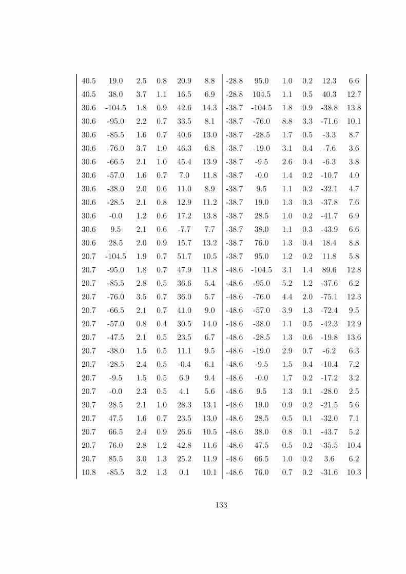
40.5 19.0 2.5 0.8 20.9 8.8 -28.8 95.0 1.0 0.2 12.3 6.6
40.5 38.0 3.7 1.1 16.5 6.9 -28.8 104.5 1.1 0.5 40.3 12.7
30.6 -104.5 1.8 0.9 42.6 14.3 -38.7 -104.5 1.8 0.9 -38.8 13.8
30.6 -95.0 2.2 0.7 33.5 8.1 -38.7 -76.0 8.8 3.3 -71.6 10.1
30.6 -85.5 1.6 0.7 40.6 13.0 -38.7 -28.5 1.7 0.5 -3.3 8.7
30.6 -76.0 3.7 1.0 46.3 6.8 -38.7 -19.0 3.1 0.4 -7.6 3.6
30.6 -66.5 2.1 1.0 45.4 13.9 -38.7 -9.5 2.6 0.4 -6.3 3.8
30.6 -57.0 1.6 0.7 7.0 11.8 -38.7 -0.0 1.4 0.2 -10.7 4.0
30.6 -38.0 2.0 0.6 11.0 8.9 -38.7 9.5 1.1 0.2 -32.1 4.7
30.6 -28.5 2.1 0.8 12.9 11.2 -38.7 19.0 1.3 0.3 -37.8 7.6
30.6 -0.0 1.2 0.6 17.2 13.8 -38.7 28.5 1.0 0.2 -41.7 6.9
30.6 9.5 2.1 0.6 -7.7 7.7 -38.7 38.0 1.1 0.3 -43.9 6.6
30.6 28.5 2.0 0.9 15.7 13.2 -38.7 76.0 1.3 0.4 18.4 8.8
20.7 -104.5 1.9 0.7 51.7 10.5 -38.7 95.0 1.2 0.2 11.8 5.8
20.7 -95.0 1.8 0.7 47.9 11.8 -48.6 -104.5 3.1 1.4 89.6 12.8
20.7 -85.5 2.8 0.5 36.6 5.4 -48.6 -95.0 5.2 1.2 -37.6 6.2
20.7 -76.0 3.5 0.7 36.0 5.7 -48.6 -76.0 4.4 2.0 -75.1 12.3
20.7 -66.5 2.1 0.7 41.0 9.0 -48.6 -57.0 3.9 1.3 -72.4 9.5
20.7 -57.0 0.8 0.4 30.5 14.0 -48.6 -38.0 1.1 0.5 -42.3 12.9
20.7 -47.5 2.1 0.5 23.5 6.7 -48.6 -28.5 1.3 0.6 -19.8 13.6
20.7 -38.0 1.5 0.5 11.1 9.5 -48.6 -19.0 2.9 0.7 -6.2 6.3
20.7 -28.5 2.4 0.5 -0.4 6.1 -48.6 -9.5 1.5 0.4 -10.4 7.2
20.7 -9.5 1.5 0.5 6.9 9.4 -48.6 -0.0 1.7 0.2 -17.2 3.2
20.7 -0.0 2.3 0.5 4.1 5.6 -48.6 9.5 1.3 0.1 -28.0 2.5
20.7 28.5 2.1 1.0 28.3 13.1 -48.6 19.0 0.9 0.2 -21.5 5.6
20.7 47.5 1.6 0.7 23.5 13.0 -48.6 28.5 0.5 0.1 -32.0 7.1
20.7 66.5 2.4 0.9 26.6 10.5 -48.6 38.0 0.8 0.1 -43.7 5.2
20.7 76.0 2.8 1.2 42.8 11.6 -48.6 47.5 0.5 0.2 -35.5 10.4
20.7 85.5 3.0 1.3 25.2 11.9 -48.6 66.5 1.0 0.2 3.6 6.2
10.8 -85.5 3.2 1.3 0.1 10.1 -48.6 76.0 0.7 0.2 -31.6 10.3
133
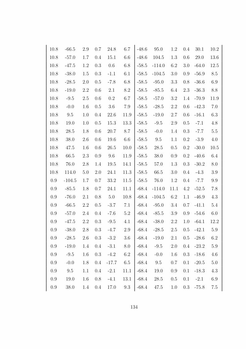
10.8 -66.5 2.9 0.7 24.8 6.7 -48.6 95.0 1.2 0.4 30.1 10.2
10.8 -57.0 1.7 0.4 15.1 6.6 -48.6 104.5 1.3 0.6 29.0 13.6
10.8 -47.5 1.2 0.3 0.6 6.8 -58.5 -114.0 6.2 3.0 -64.0 12.5
10.8 -38.0 1.5 0.3 -1.1 6.1 -58.5 -104.5 3.0 0.9 -56.9 8.5
10.8 -28.5 2.0 0.5 -7.8 6.8 -58.5 -95.0 3.3 0.8 -36.6 6.9
10.8 -19.0 2.2 0.6 2.1 8.2 -58.5 -85.5 6.4 2.3 -36.3 8.8
10.8 -9.5 2.5 0.6 0.2 6.7 -58.5 -57.0 3.2 1.4 -70.9 11.9
10.8 -0.0 1.6 0.5 3.6 7.9 -58.5 -28.5 2.2 0.6 -42.3 7.0
10.8 9.5 1.0 0.4 22.6 11.9 -58.5 -19.0 2.7 0.6 -16.1 6.3
10.8 19.0 1.0 0.5 15.3 13.3 -58.5 -9.5 2.9 0.5 -7.1 4.8
10.8 28.5 1.8 0.6 20.7 8.7 -58.5 -0.0 1.4 0.3 -7.7 5.5
10.8 38.0 2.6 0.6 19.6 6.6 -58.5 9.5 1.1 0.2 -3.9 4.0
10.8 47.5 1.6 0.6 26.5 10.0 -58.5 28.5 0.5 0.2 -30.0 10.5
10.8 66.5 2.3 0.9 9.6 11.9 -58.5 38.0 0.9 0.2 -40.6 6.4
10.8 76.0 2.8 1.4 19.5 14.1 -58.5 57.0 1.3 0.3 -30.2 8.0
10.8 114.0 5.0 2.0 24.1 11.3 -58.5 66.5 3.0 0.4 -4.3 3.9
0.9 -104.5 1.7 0.7 33.2 11.5 -58.5 76.0 1.2 0.4 -7.7 9.9
0.9 -85.5 1.8 0.7 24.1 11.1 -68.4 -114.0 11.1 4.2 -52.5 7.8
0.9 -76.0 2.1 0.8 5.0 10.8 -68.4 -104.5 6.2 1.1 -46.9 4.3
0.9 -66.5 2.2 0.5 -3.7 7.1 -68.4 -95.0 3.4 0.7 -41.1 5.4
0.9 -57.0 2.4 0.4 -7.6 5.2 -68.4 -85.5 3.9 0.9 -54.6 6.0
0.9 -47.5 2.2 0.3 -9.5 4.1 -68.4 -38.0 2.2 1.0 -64.1 12.2
0.9 -38.0 2.8 0.3 -4.7 2.9 -68.4 -28.5 2.5 0.5 -42.1 5.9
0.9 -28.5 2.6 0.3 -3.2 3.6 -68.4 -19.0 2.1 0.5 -28.6 6.2
0.9 -19.0 1.4 0.4 -3.1 8.0 -68.4 -9.5 2.0 0.4 -23.2 5.9
0.9 -9.5 1.6 0.3 -4.2 6.2 -68.4 -0.0 1.6 0.3 -18.6 4.6
0.9 -0.0 1.8 0.4 -17.7 6.5 -68.4 9.5 0.7 0.1 -20.5 5.0
0.9 9.5 1.1 0.4 -2.1 11.1 -68.4 19.0 0.9 0.1 -18.3 4.3
0.9 19.0 1.6 0.8 -4.1 13.1 -68.4 28.5 0.5 0.1 -2.1 6.9
0.9 38.0 1.4 0.4 17.0 9.3 -68.4 47.5 1.0 0.3 -75.8 7.5
134
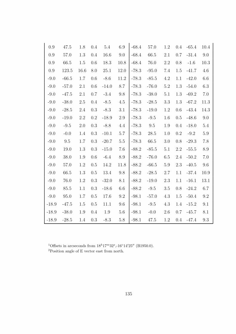
0.9 47.5 1.8 0.4 5.4 6.9 -68.4 57.0 1.2 0.4 -65.4 10.4
0.9 57.0 1.3 0.4 16.6 9.0 -68.4 66.5 2.1 0.7 -31.4 9.0
0.9 66.5 1.5 0.6 18.3 10.8 -68.4 76.0 2.2 0.8 -1.6 10.3
0.9 123.5 16.6 8.0 25.1 12.0 -78.3 -95.0 7.4 1.5 -41.7 4.6
-9.0 -66.5 1.7 0.6 -8.6 11.2 -78.3 -85.5 4.2 1.1 -42.0 6.6
-9.0 -57.0 2.1 0.6 -14.0 8.7 -78.3 -76.0 5.2 1.3 -54.0 6.3
-9.0 -47.5 2.1 0.7 -3.4 9.8 -78.3 -38.0 5.1 1.3 -69.2 7.0
-9.0 -38.0 2.5 0.4 -8.5 4.5 -78.3 -28.5 3.3 1.3 -67.2 11.3
-9.0 -28.5 2.4 0.3 -8.3 3.1 -78.3 -19.0 1.2 0.6 -43.4 14.3
-9.0 -19.0 2.2 0.2 -18.9 2.9 -78.3 -9.5 1.6 0.5 -48.6 9.0
-9.0 -9.5 2.0 0.3 -8.8 4.4 -78.3 9.5 1.9 0.4 -18.0 5.4
-9.0 -0.0 1.4 0.3 -10.1 5.7 -78.3 28.5 1.0 0.2 -9.2 5.9
-9.0 9.5 1.7 0.3 -20.7 5.5 -78.3 66.5 3.0 0.8 -29.3 7.8
-9.0 19.0 1.3 0.3 -15.0 7.6 -88.2 -85.5 5.1 2.2 -55.5 8.9
-9.0 38.0 1.9 0.6 -6.4 8.9 -88.2 -76.0 6.5 2.4 -50.2 7.0
-9.0 57.0 1.2 0.5 14.2 11.8 -88.2 -66.5 5.9 2.3 -40.5 9.6
-9.0 66.5 1.3 0.5 13.4 9.8 -88.2 -28.5 2.7 1.1 -37.4 10.9
-9.0 76.0 1.2 0.3 -32.0 8.1 -88.2 -19.0 2.3 1.1 -16.1 13.1
-9.0 85.5 1.1 0.3 -18.6 6.6 -88.2 -9.5 3.5 0.8 -24.2 6.7
-9.0 95.0 1.7 0.5 17.6 9.2 -98.1 -57.0 4.3 1.5 -50.4 9.2
-18.9 -47.5 1.5 0.5 11.1 9.6 -98.1 -9.5 4.3 1.4 -15.2 9.1
-18.9 -38.0 1.9 0.4 1.9 5.6 -98.1 -0.0 2.6 0.7 -45.7 8.1
-18.9 -28.5 1.4 0.3 -8.3 5.8 -98.1 47.5 1.2 0.4 -47.4 9.3
1Offsets in arcseconds from 18h17m32s,-1614′25′′ (B1950.0).2Position angle of E vector east from north.
135
Appendix B
Blackbody Radiation
All matter emits electromagnetic radiation when it has a temperature above ab-
solute zero. A black body is an idealized physical body that absorbs all incident
radiation. Because of this perfect absorptivity at all wavelengths, a black body is
also the best emitter of thermal radiation, which it radiates incandescently in a char-
acteristic, continuous spectrum that depends on the body’s temperature.
The thermal radiation from a black body is called black body radiation. Planck’s
law describes the radiation from a black body with a temperature of T:
Bν(T ) =2hν3
c21
ehν/(kT ) − 1(B.1)
Where h is Planck’s constant, c is the speed of light, k is Boltzmann’s constant
and Bν(T ) is in the unit of Js−1m−2sr−1Hz−1.
In the Wien limit, where hν ≫ kT , the Plank’s spectrum is approximately:
Bν(T ) ≈2hν3
c2e−hν/(kT ) (B.2)
At low frequency range, where hν ≪ kT (Rayleigh-Jeans limit), it is approxi-
mately:
Bν(T ) ≈ 2kTν2/c2 (B.3)
Figure B.1 shows the Plank spectrum, Wien limit and Rayleigh-Jeans limit of a
black body with a temperature of 2.725K. The black body radiation spectrum peaks
136
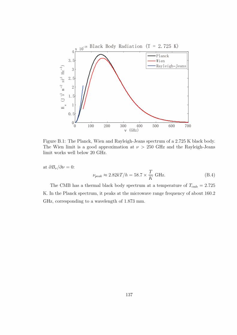
−
ν
ν
−−
−−
−
Figure B.1: The Planck, Wien and Rayleigh-Jeans spectrum of a 2.725 K black body.The Wien limit is a good approximation at ν > 250 GHz and the Rayleigh-Jeanslimit works well below 20 GHz.
at ∂Bν/∂ν = 0:
νpeak ≈ 2.82kT/h = 58.7× T
KGHz. (B.4)
The CMB has a thermal black body spectrum at a temperature of Tcmb = 2.725
K. In the Planck spectrum, it peaks at the microwave range frequency of about 160.2
GHz, corresponding to a wavelength of 1.873 mm.
137
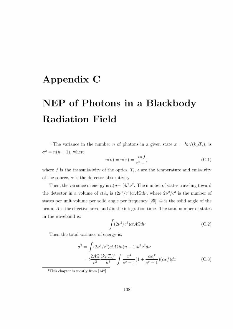
Appendix C
NEP of Photons in a Blackbody
Radiation Field
1 The variance in the number n of photons in a given state x = hν/(kBTs), is
σ2 = n(n+ 1), where
n(ν) = n(x) =αǫf
ex − 1(C.1)
where f is the transmissivity of the optics, Ts, ǫ are the temperature and emissivity
of the source, α is the detector absorptivity.
Then, the variance in energy is n(n+1)h2ν2. The number of states traveling toward
the detector in a volume of ctA, is (2ν2/c3)ctAΩdν, where 2ν2/c3 is the number of
states per unit volume per solid angle per frequency [25], Ω is the solid angle of the
beam, A is the effective area, and t is the integration time. The total number of states
in the waveband is:∫
(2ν2/c3)ctAΩdν (C.2)
Then the total variance of energy is:
σ2 =
∫
(2ν2/c3)ctAΩn(n + 1)h2ν2dν
= t2AΩ
c2(kBTs)
5
h3
∫
x4
ex − 1(1 +
αǫf
ex − 1)(αǫf)dx (C.3)
1This chapter is mostly from [142]
138
NEP is defined as the error in power in a half-second integration (section 4.2.1):
NEP2 =2σ2
t
=4AΩ
c2(kBTs)
5
h3
∫
x4
ex − 1(1 +
αǫf
ex − 1)(αǫf)dx (C.4)
NEP has the unit of W2Hz−1/2.
139
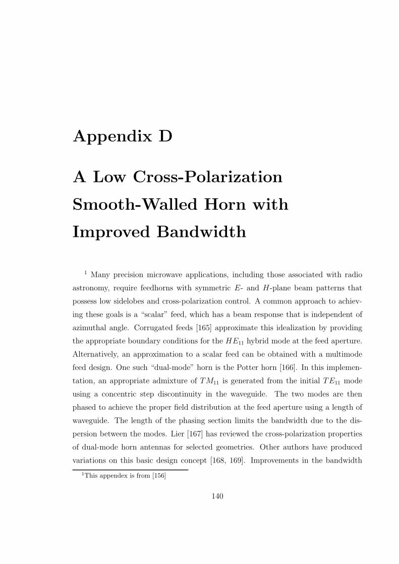
Appendix D
A Low Cross-Polarization
Smooth-Walled Horn with
Improved Bandwidth
1 Many precision microwave applications, including those associated with radio
astronomy, require feedhorns with symmetric E- and H-plane beam patterns that
possess low sidelobes and cross-polarization control. A common approach to achiev-
ing these goals is a “scalar” feed, which has a beam response that is independent of
azimuthal angle. Corrugated feeds [165] approximate this idealization by providing
the appropriate boundary conditions for the HE11 hybrid mode at the feed aperture.
Alternatively, an approximation to a scalar feed can be obtained with a multimode
feed design. One such “dual-mode” horn is the Potter horn [166]. In this implemen-
tation, an appropriate admixture of TM11 is generated from the initial TE11 mode
using a concentric step discontinuity in the waveguide. The two modes are then
phased to achieve the proper field distribution at the feed aperture using a length of
waveguide. The length of the phasing section limits the bandwidth due to the dis-
persion between the modes. Lier [167] has reviewed the cross-polarization properties
of dual-mode horn antennas for selected geometries. Other authors have produced
variations on this basic design concept [168, 169]. Improvements in the bandwidth
1This appendex is from [156]
140
have been realized by decreasing the phase difference between the two modes by 2π
[170, 171].
To increase the bandwidth, it is possible to add multiple concentric step continu-
ities with the appropriate modal phasing [172, 173]. A variation on this technique is
to use several distinct linear tapers to generate the proper modal content and phasing
[174, 175]. Operational bandwidths of 15-20% have been reported using such tech-
niques. A related class of devices is realized by allowing the feedhorn profile to vary
smoothly rather than in discrete steps. Examples of such smooth-walled feedhorns
with ∼15% fractional bandwidths exist in the literature [162, 176].
In this work, we describe the design and optimization of a smooth-walled feed that
has a 30% operational bandwidth, over which the cross-polarization response is better
than -30 dB. The optimization technique is described, and the performance of the feed
is compared with other published dual-mode feedhorns. The feedhorn described here
has a monotonic profile that allows it to be manufactured by progressively milling
the profile using a set of custom tools.
D.1 Smooth-walled Feedhorn Optimization
The performance of a feedhorn can be characterized by angle- and frequency-
dependent quantities that include beam width, sidelobe response and cross-polarization.
Quantities such as reflection coefficient and polarization isolation that only depend
on frequency are also important considerations. All of these functions are dependent
upon the shape of the feed profile. In the optimization approach described, a weighted
penalty function is used to explore and optimize the relationship between the feed
profile and the electromagnetic response.
D.1.1 Beam Response Calculation
The smooth-walled horn was approximated by a profile that consists of discrete
waveguide sections, each of constant radius. With this approach, it was important
to verify that each section is thin enough that the model is a valid approximation of
141
the continuous profile. For profiles relevant to our design parameters, section lengths
of ∆l ≤ λc/20 were found to be sufficient by trial and error, where λc is the cutoff
wavelength of the input waveguide section. It is possible in principle to dynamically
set the length of each section to optimize the approximation to the local curvature of
the horn. This would increase the speed of the optimization; however, for simplicity,
this detail was not implemented in our study.
For each trial feedhorn the angular response was calculated directly from the modal
content at the feed aperture. This in turn was calculated as follows. The throat
of the feedhorn was assumed to be excited by the circular waveguide TE11 mode.
The modal content of each successive section was then determined by matching the
boundary conditions at each interface using the method of James [18]. The cylindrical
symmetry of the feed limits the possible propagating modes to those with the same
azimuthal functional form as TE11 [177]. This azimuthal-dependence extends to
the resulting beam patterns, allowing the full beam pattern to be calculated from
the E- and H- plane angular response. Ludwig’s third definition [178] is employed
in calculation and measurement of cross-polar response. We note that an additional
consequence of the feedhorn symmetry is that to the extent that the E- and H-planes
are equal in both phase and amplitude, the cross-polarization is zero [159]. Changes
in curvature in the feed profile can excite higher order modes (e.g., TE12 and TM12),
the presence of which can potentially degrade the cross-polarization response of the
horn.
D.1.2 Penalty Function
We constructed a penalty function to optimize the antenna profile. The penalty
function with normalized weights, αj , is written as
χ2 =
N∑
i=1
M∑
j=1
(
αj∆j(fi)2)
, (D.1)
where i sums over a discrete set of (N) frequencies in the optimization frequency
band, and j sums over the number (M) of discrete parameters one wishes to take
into account for the optimization. In the parameter space considered, this function
142
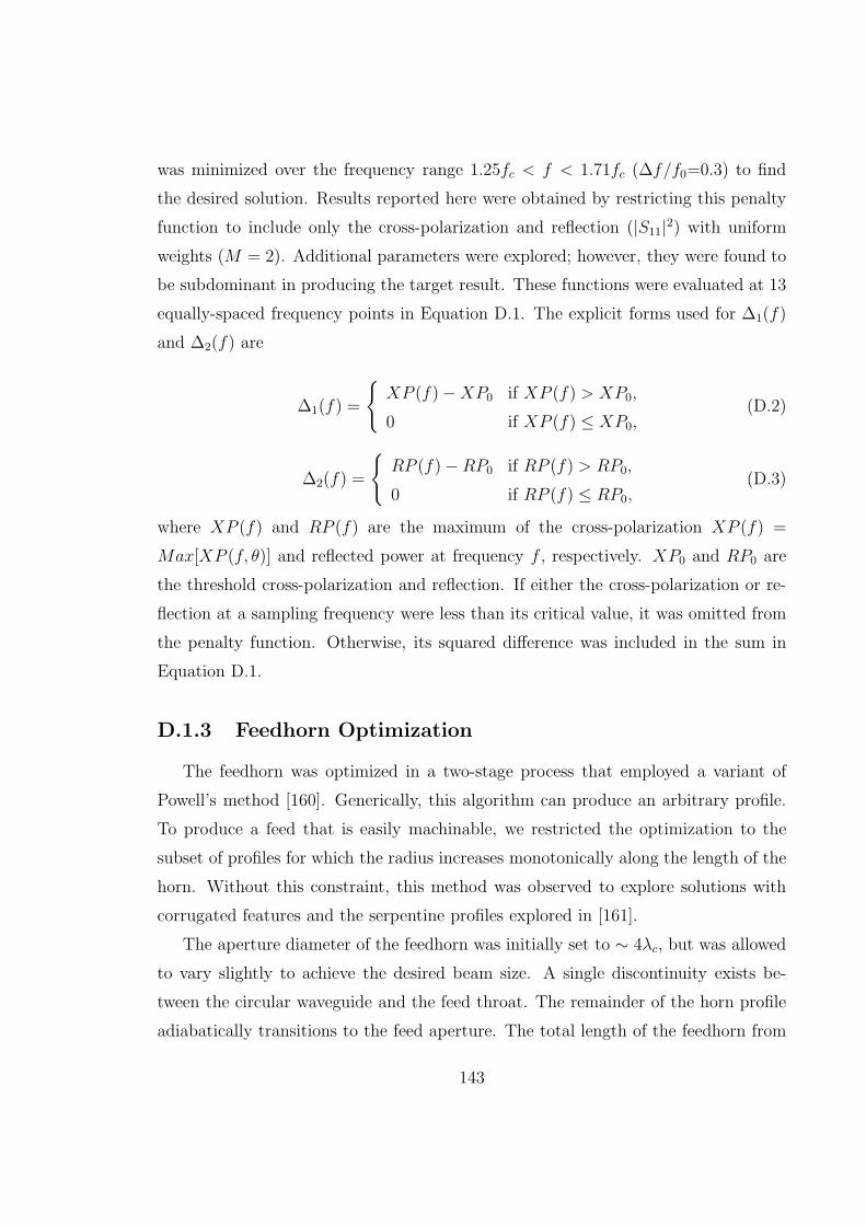
was minimized over the frequency range 1.25fc < f < 1.71fc (∆f/f0=0.3) to find
the desired solution. Results reported here were obtained by restricting this penalty
function to include only the cross-polarization and reflection (|S11|2) with uniform
weights (M = 2). Additional parameters were explored; however, they were found to
be subdominant in producing the target result. These functions were evaluated at 13
equally-spaced frequency points in Equation D.1. The explicit forms used for ∆1(f)
and ∆2(f) are
∆1(f) =
XP (f)−XP0 if XP (f) > XP0,
0 if XP (f) ≤ XP0,(D.2)
∆2(f) =
RP (f)− RP0 if RP (f) > RP0,
0 if RP (f) ≤ RP0,(D.3)
where XP (f) and RP (f) are the maximum of the cross-polarization XP (f) =
Max[XP (f, θ)] and reflected power at frequency f , respectively. XP0 and RP0 are
the threshold cross-polarization and reflection. If either the cross-polarization or re-
flection at a sampling frequency were less than its critical value, it was omitted from
the penalty function. Otherwise, its squared difference was included in the sum in
Equation D.1.
D.1.3 Feedhorn Optimization
The feedhorn was optimized in a two-stage process that employed a variant of
Powell’s method [160]. Generically, this algorithm can produce an arbitrary profile.
To produce a feed that is easily machinable, we restricted the optimization to the
subset of profiles for which the radius increases monotonically along the length of the
horn. Without this constraint, this method was observed to explore solutions with
corrugated features and the serpentine profiles explored in [161].
The aperture diameter of the feedhorn was initially set to ∼ 4λc, but was allowed
to vary slightly to achieve the desired beam size. A single discontinuity exists be-
tween the circular waveguide and the feed throat. The remainder of the horn profile
adiabatically transitions to the feed aperture. The total length of the feedhorn from
143
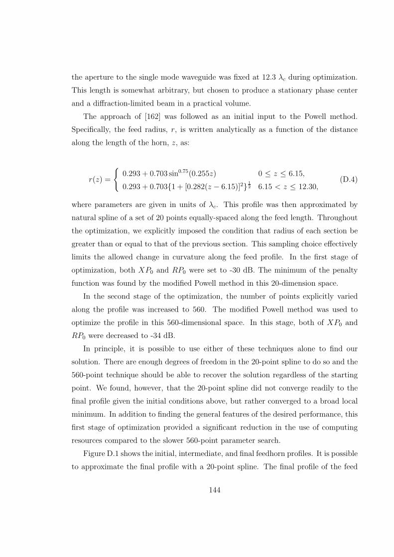
the aperture to the single mode waveguide was fixed at 12.3 λc during optimization.
This length is somewhat arbitrary, but chosen to produce a stationary phase center
and a diffraction-limited beam in a practical volume.
The approach of [162] was followed as an initial input to the Powell method.
Specifically, the feed radius, r, is written analytically as a function of the distance
along the length of the horn, z, as:
r(z) =
0.293 + 0.703 sin0.75(0.255z) 0 ≤ z ≤ 6.15,
0.293 + 0.7031 + [0.282(z − 6.15)]2 12 6.15 < z ≤ 12.30,
(D.4)
where parameters are given in units of λc. This profile was then approximated by
natural spline of a set of 20 points equally-spaced along the feed length. Throughout
the optimization, we explicitly imposed the condition that radius of each section be
greater than or equal to that of the previous section. This sampling choice effectively
limits the allowed change in curvature along the feed profile. In the first stage of
optimization, both XP0 and RP0 were set to -30 dB. The minimum of the penalty
function was found by the modified Powell method in this 20-dimension space.
In the second stage of the optimization, the number of points explicitly varied
along the profile was increased to 560. The modified Powell method was used to
optimize the profile in this 560-dimensional space. In this stage, both of XP0 and
RP0 were decreased to -34 dB.
In principle, it is possible to use either of these techniques alone to find our
solution. There are enough degrees of freedom in the 20-point spline to do so and the
560-point technique should be able to recover the solution regardless of the starting
point. We found, however, that the 20-point spline did not converge readily to the
final profile given the initial conditions above, but rather converged to a broad local
minimum. In addition to finding the general features of the desired performance, this
first stage of optimization provided a significant reduction in the use of computing
resources compared to the slower 560-point parameter search.
Figure D.1 shows the initial, intermediate, and final feedhorn profiles. It is possible
to approximate the final profile with a 20-point spline. The final profile of the feed
144
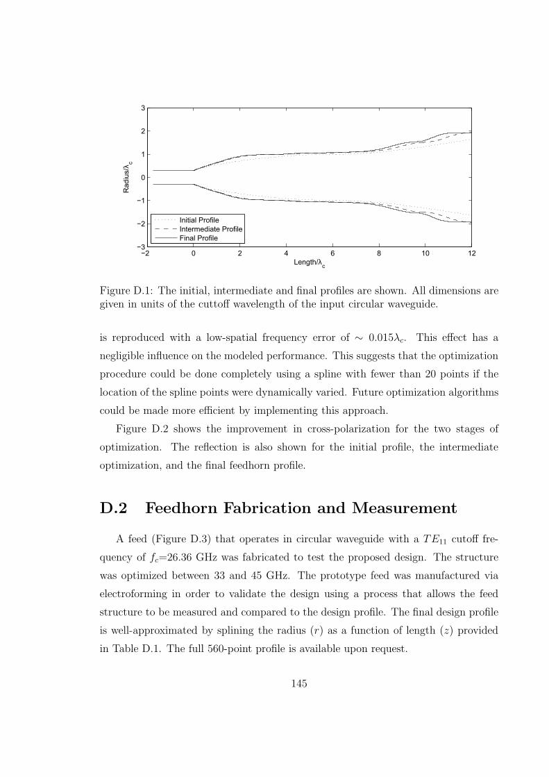
−2 0 2 4 6 8 10 12−3
−2
−1
0
1
2
3
Rad
ius/
λ c
Length/λc
Initial ProfileIntermediate ProfileFinal Profile
Figure D.1: The initial, intermediate and final profiles are shown. All dimensions aregiven in units of the cuttoff wavelength of the input circular waveguide.
is reproduced with a low-spatial frequency error of ∼ 0.015λc. This effect has a
negligible influence on the modeled performance. This suggests that the optimization
procedure could be done completely using a spline with fewer than 20 points if the
location of the spline points were dynamically varied. Future optimization algorithms
could be made more efficient by implementing this approach.
Figure D.2 shows the improvement in cross-polarization for the two stages of
optimization. The reflection is also shown for the initial profile, the intermediate
optimization, and the final feedhorn profile.
D.2 Feedhorn Fabrication and Measurement
A feed (Figure D.3) that operates in circular waveguide with a TE11 cutoff fre-
quency of fc=26.36 GHz was fabricated to test the proposed design. The structure
was optimized between 33 and 45 GHz. The prototype feed was manufactured via
electroforming in order to validate the design using a process that allows the feed
structure to be measured and compared to the design profile. The final design profile
is well-approximated by splining the radius (r) as a function of length (z) provided
in Table D.1. The full 560-point profile is available upon request.
145
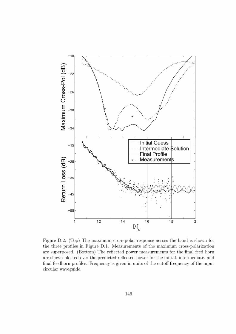
−34
−30
−26
−22
−18
Ret
urn
Loss
(dB
)
1 1.2 1.4 1.6 1.8 2
−55
−45
−35
−25
−15
Max
imum
Cro
ss-P
ol (d
B)
Final ProfileIntermediate Solution
Measurements
Initial Guess
f/fc
Figure D.2: (Top) The maximum cross-polar response across the band is shown forthe three profiles in Figure D.1. Measurements of the maximum cross-polarizationare superposed. (Bottom) The reflected power measurements for the final feed hornare shown plotted over the predicted reflected power for the initial, intermediate, andfinal feedhorn profiles. Frequency is given in units of the cutoff frequency of the inputcircular waveguide.
146
The feedhorn was measured in the Goddard Electromagnetic Anechoic Chamber
(GEMAC). The receivers and microwave sources used in the measurement provide
a > 50 dB dynamic range from the peak response over ∼ 2π steradians with an
absolute accuracy of < 0.5 dB. A five section constant cutoff transition from rect-
angular waveguide (WR 22.4, fc = 26.36 GHz) to circular waveguide [179] was used
to mate the feedhorn to the rectangular waveguide of the antenna range infrastruc-
ture. The constant cutoff condition was maintained in the transition by ensuring
acircle = abroadwalls11/π where acircle is the radius of the circular guide, abroadwall is the
width of the broadwall of the rectangular guide, and s11 ∼ 1.841 is the eigenvalue
for the TE11 mode [158]. The alignment of the circular waveguide feed interface was
maintained to avoid degradation of the cross-polar antenna response. Pinning of this
interface as specified in [180] or similar is recommended.
Beam plots and parameters at the extrema and the middle of the optimization
frequency range are shown in Figure D.4 and Table D.2. The cross-polarization
response as a function of frequency of this device is compared to other published
implementations of multi-mode scalar feeds (Fig. D.5). As is common for applications
requiring the beam symmetry provided by a scalar horn, the aperture efficiency is low.
In addition, we note that the phase center for this horn is near the aperture and is
stable in frequency.
An HP8510C network analzyer was used to measure the reflected power (see Fig.
D.2) with a through-reflect-line calibration in circular waveguide. If desired, the
match at the lower band edge can be improved by using a transition to a larger
diameter guide. The measured observations are in agreement with theory.
Imperfections in the profile may occur during manufacturing due to chattering of
the tooling or similar physical processes. We performed a tolerance study to deter-
mine the effect of such high-spatial frequency errors in the feed radius. Negligible
degradation in performance was observed for Gaussian errors in the radius up to
0.002 λc. The feed’s monotonic profile is compatible with machining by progressive
plunge milling in which successively more accurate tools are used to realize the feed
profile. This technique has been used for individual feeds and is potentially useful
for fabricating large arrays of feedhorns. Examples include fabrication of multimode
147
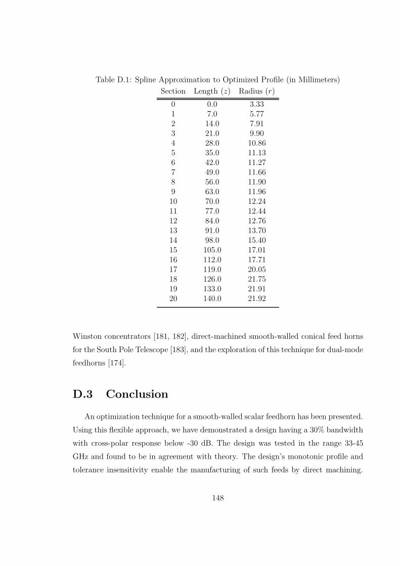
Table D.1: Spline Approximation to Optimized Profile (in Millimeters)
Section Length (z) Radius (r)
0 0.0 3.331 7.0 5.772 14.0 7.913 21.0 9.904 28.0 10.865 35.0 11.136 42.0 11.277 49.0 11.668 56.0 11.909 63.0 11.9610 70.0 12.2411 77.0 12.4412 84.0 12.7613 91.0 13.7014 98.0 15.4015 105.0 17.0116 112.0 17.7117 119.0 20.0518 126.0 21.7519 133.0 21.9120 140.0 21.92
Winston concentrators [181, 182], direct-machined smooth-walled conical feed horns
for the South Pole Telescope [183], and the exploration of this technique for dual-mode
feedhorns [174].
D.3 Conclusion
An optimization technique for a smooth-walled scalar feedhorn has been presented.
Using this flexible approach, we have demonstrated a design having a 30% bandwidth
with cross-polar response below -30 dB. The design was tested in the range 33-45
GHz and found to be in agreement with theory. The design’s monotonic profile and
tolerance insensitivity enable the manufacturing of such feeds by direct machining.
148
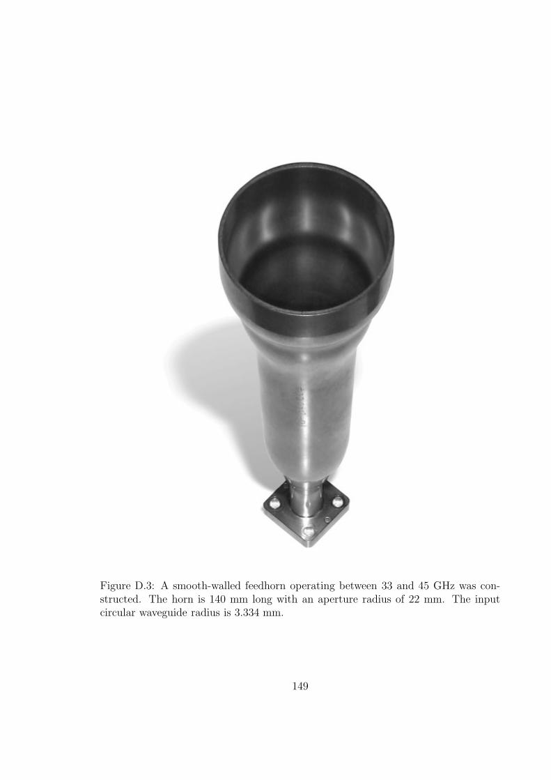
Figure D.3: A smooth-walled feedhorn operating between 33 and 45 GHz was con-structed. The horn is 140 mm long with an aperture radius of 22 mm. The inputcircular waveguide radius is 3.334 mm.
149
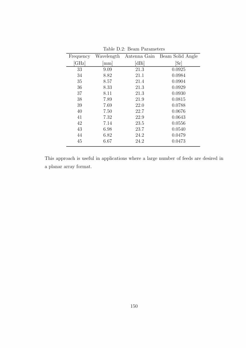
Table D.2: Beam Parameters
Frequency Wavelength Antenna Gain Beam Solid Angle
[GHz] [mm] [dBi] [Sr]33 9.09 21.3 0.092534 8.82 21.1 0.098435 8.57 21.4 0.090436 8.33 21.3 0.092937 8.11 21.3 0.093038 7.89 21.9 0.081539 7.69 22.0 0.078840 7.50 22.7 0.067641 7.32 22.9 0.064342 7.14 23.5 0.055643 6.98 23.7 0.054044 6.82 24.2 0.047945 6.67 24.2 0.0473
This approach is useful in applications where a large number of feeds are desired in
a planar array format.
150
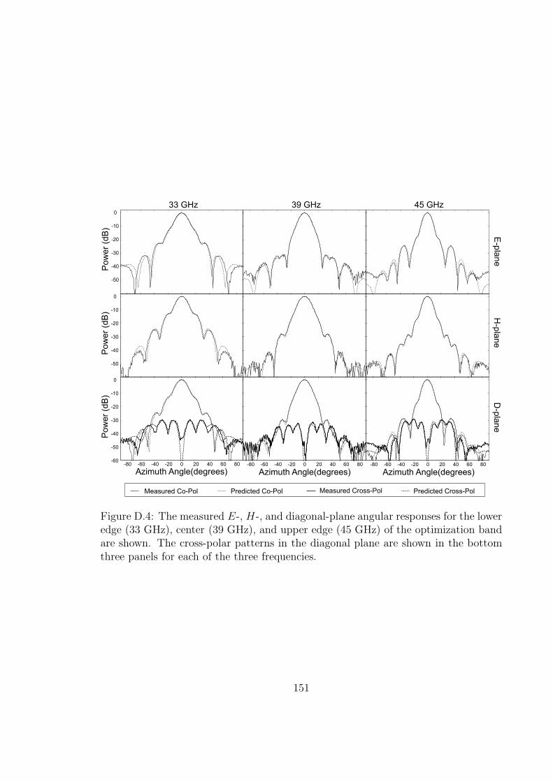
-50
-40
-30
-20
-10
0
Pow
er (d
B)
33 GHz
39 GHz
45 GHz
-50
-40
-30
-20
-10
0
Pow
er (d
B)
-80 -60 -40 -20 0 20 40 60 80Azimuth Angle(degrees)
-60
-50
-40
-30
-20
-10
0
Pow
er (d
B)
-80 -60 -40 -20 0 20 40 60 80
Azimuth Angle(degrees)-80 -60 -40 -20 0 20 40 60 80
Azimuth Angle(degrees)
Measured Co-Pol Predicted Co-Pol Measured Cross-Pol Predicted Cross-Pol
E-plane
H-plane
D-plane
Figure D.4: The measured E-, H-, and diagonal-plane angular responses for the loweredge (33 GHz), center (39 GHz), and upper edge (45 GHz) of the optimization bandare shown. The cross-polar patterns in the diagonal plane are shown in the bottomthree panels for each of the three frequencies.
151
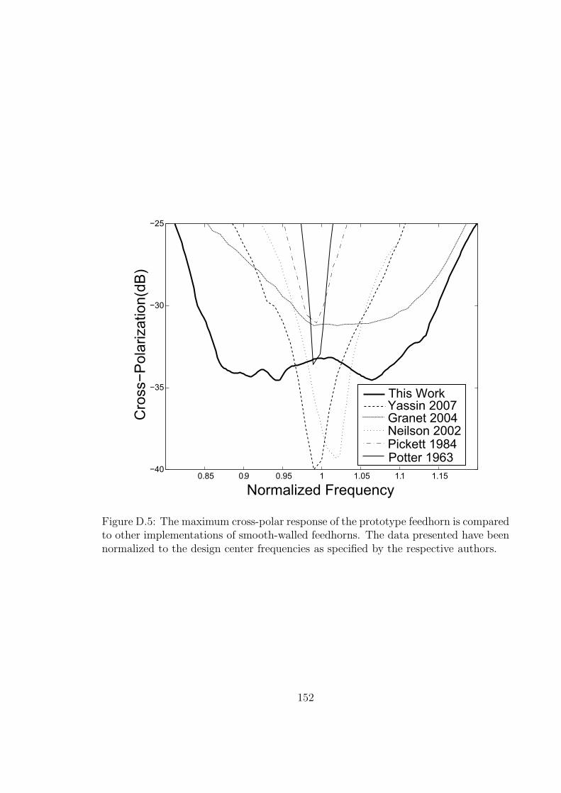
0.85 0.9 0.95 1 1.05 1.1 1.15−40
−35
−30
−25
Normalized Frequency
Cro
ss−P
olar
izat
ion(
dB)
This WorkYassin 2007Granet 2004Neilson 2002Pickett 1984Potter 1963
Figure D.5: The maximum cross-polar response of the prototype feedhorn is comparedto other implementations of smooth-walled feedhorns. The data presented have beennormalized to the design center frequencies as specified by the respective authors.
152
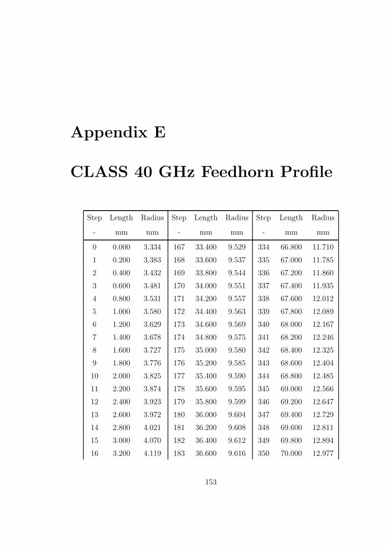
Appendix E
CLASS 40 GHz Feedhorn Profile
Step Length Radius Step Length Radius Step Length Radius
- mm mm - mm mm - mm mm
0 0.000 3.334 167 33.400 9.529 334 66.800 11.710
1 0.200 3.383 168 33.600 9.537 335 67.000 11.785
2 0.400 3.432 169 33.800 9.544 336 67.200 11.860
3 0.600 3.481 170 34.000 9.551 337 67.400 11.935
4 0.800 3.531 171 34.200 9.557 338 67.600 12.012
5 1.000 3.580 172 34.400 9.563 339 67.800 12.089
6 1.200 3.629 173 34.600 9.569 340 68.000 12.167
7 1.400 3.678 174 34.800 9.575 341 68.200 12.246
8 1.600 3.727 175 35.000 9.580 342 68.400 12.325
9 1.800 3.776 176 35.200 9.585 343 68.600 12.404
10 2.000 3.825 177 35.400 9.590 344 68.800 12.485
11 2.200 3.874 178 35.600 9.595 345 69.000 12.566
12 2.400 3.923 179 35.800 9.599 346 69.200 12.647
13 2.600 3.972 180 36.000 9.604 347 69.400 12.729
14 2.800 4.021 181 36.200 9.608 348 69.600 12.811
15 3.000 4.070 182 36.400 9.612 349 69.800 12.894
16 3.200 4.119 183 36.600 9.616 350 70.000 12.977
153
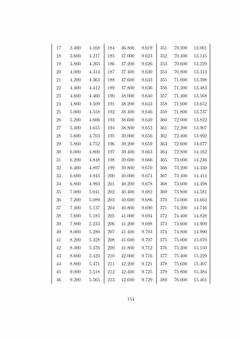
17 3.400 4.168 184 36.800 9.619 351 70.200 13.061
18 3.600 4.217 185 37.000 9.623 352 70.400 13.145
19 3.800 4.265 186 37.200 9.626 353 70.600 13.229
20 4.000 4.314 187 37.400 9.630 354 70.800 13.313
21 4.200 4.363 188 37.600 9.633 355 71.000 13.398
22 4.400 4.412 189 37.800 9.636 356 71.200 13.483
23 4.600 4.460 190 38.000 9.640 357 71.400 13.568
24 4.800 4.509 191 38.200 9.643 358 71.600 13.652
25 5.000 4.558 192 38.400 9.646 359 71.800 13.737
26 5.200 4.606 193 38.600 9.649 360 72.000 13.822
27 5.400 4.655 194 38.800 9.653 361 72.200 13.907
28 5.600 4.703 195 39.000 9.656 362 72.400 13.992
29 5.800 4.752 196 39.200 9.659 363 72.600 14.077
30 6.000 4.800 197 39.400 9.663 364 72.800 14.162
31 6.200 4.848 198 39.600 9.666 365 73.000 14.246
32 6.400 4.897 199 39.800 9.670 366 73.200 14.330
33 6.600 4.945 200 40.000 9.674 367 73.400 14.414
34 6.800 4.993 201 40.200 9.678 368 73.600 14.498
35 7.000 5.041 202 40.400 9.682 369 73.800 14.581
36 7.200 5.089 203 40.600 9.686 370 74.000 14.664
37 7.400 5.137 204 40.800 9.690 371 74.200 14.746
38 7.600 5.185 205 41.000 9.694 372 74.400 14.828
39 7.800 5.233 206 41.200 9.698 373 74.600 14.909
40 8.000 5.280 207 41.400 9.703 374 74.800 14.990
41 8.200 5.328 208 41.600 9.707 375 75.000 15.070
42 8.400 5.376 209 41.800 9.712 376 75.200 15.150
43 8.600 5.423 210 42.000 9.716 377 75.400 15.229
44 8.800 5.471 211 42.200 9.721 378 75.600 15.307
45 9.000 5.518 212 42.400 9.725 379 75.800 15.384
46 9.200 5.565 213 42.600 9.729 380 76.000 15.461
154
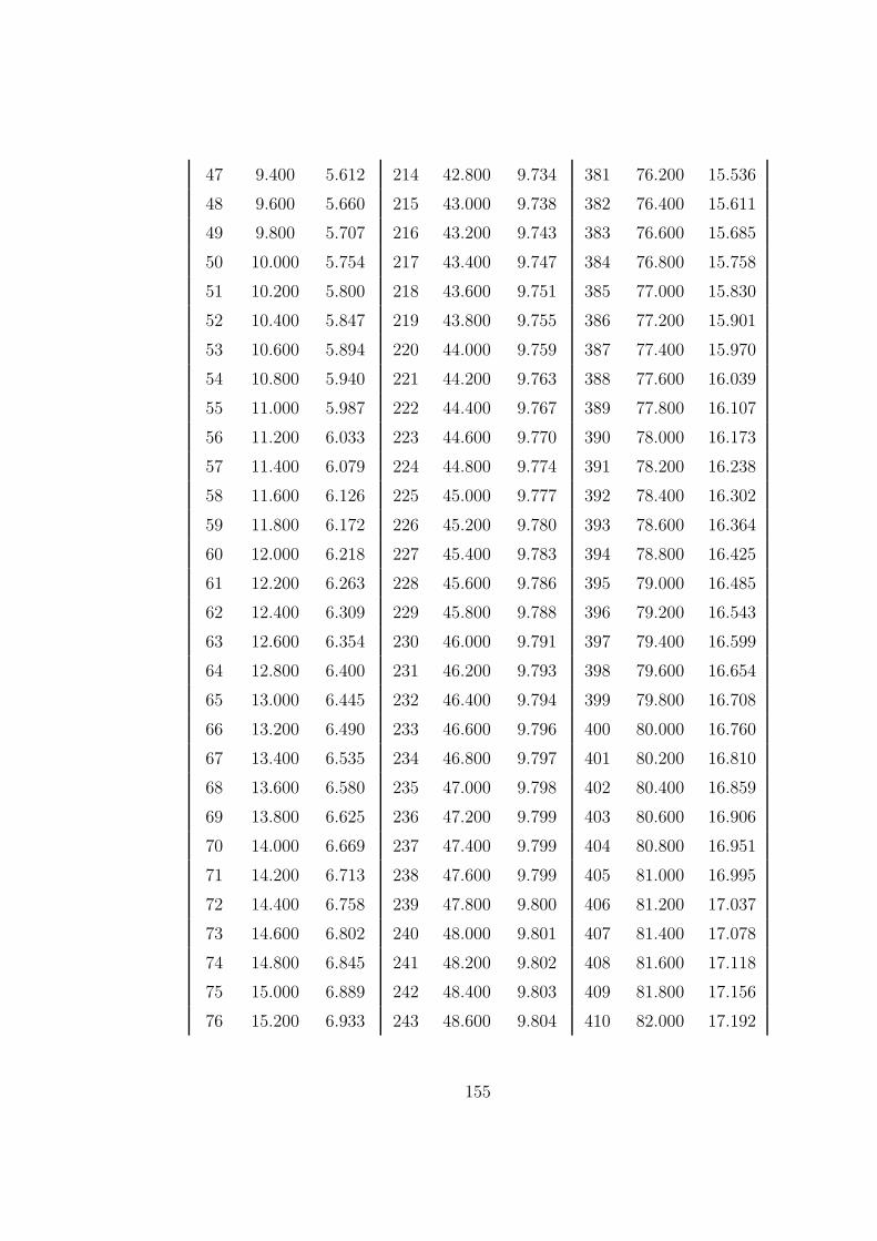
47 9.400 5.612 214 42.800 9.734 381 76.200 15.536
48 9.600 5.660 215 43.000 9.738 382 76.400 15.611
49 9.800 5.707 216 43.200 9.743 383 76.600 15.685
50 10.000 5.754 217 43.400 9.747 384 76.800 15.758
51 10.200 5.800 218 43.600 9.751 385 77.000 15.830
52 10.400 5.847 219 43.800 9.755 386 77.200 15.901
53 10.600 5.894 220 44.000 9.759 387 77.400 15.970
54 10.800 5.940 221 44.200 9.763 388 77.600 16.039
55 11.000 5.987 222 44.400 9.767 389 77.800 16.107
56 11.200 6.033 223 44.600 9.770 390 78.000 16.173
57 11.400 6.079 224 44.800 9.774 391 78.200 16.238
58 11.600 6.126 225 45.000 9.777 392 78.400 16.302
59 11.800 6.172 226 45.200 9.780 393 78.600 16.364
60 12.000 6.218 227 45.400 9.783 394 78.800 16.425
61 12.200 6.263 228 45.600 9.786 395 79.000 16.485
62 12.400 6.309 229 45.800 9.788 396 79.200 16.543
63 12.600 6.354 230 46.000 9.791 397 79.400 16.599
64 12.800 6.400 231 46.200 9.793 398 79.600 16.654
65 13.000 6.445 232 46.400 9.794 399 79.800 16.708
66 13.200 6.490 233 46.600 9.796 400 80.000 16.760
67 13.400 6.535 234 46.800 9.797 401 80.200 16.810
68 13.600 6.580 235 47.000 9.798 402 80.400 16.859
69 13.800 6.625 236 47.200 9.799 403 80.600 16.906
70 14.000 6.669 237 47.400 9.799 404 80.800 16.951
71 14.200 6.713 238 47.600 9.799 405 81.000 16.995
72 14.400 6.758 239 47.800 9.800 406 81.200 17.037
73 14.600 6.802 240 48.000 9.801 407 81.400 17.078
74 14.800 6.845 241 48.200 9.802 408 81.600 17.118
75 15.000 6.889 242 48.400 9.803 409 81.800 17.156
76 15.200 6.933 243 48.600 9.804 410 82.000 17.192
155
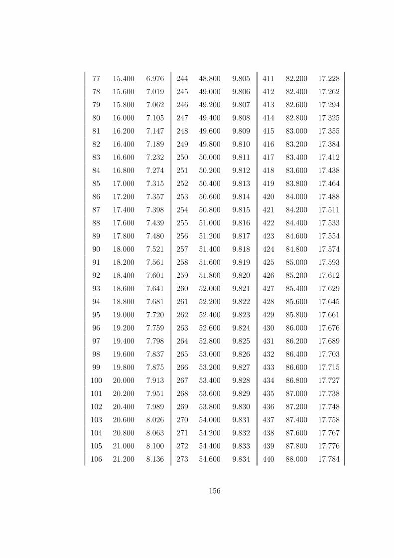
77 15.400 6.976 244 48.800 9.805 411 82.200 17.228
78 15.600 7.019 245 49.000 9.806 412 82.400 17.262
79 15.800 7.062 246 49.200 9.807 413 82.600 17.294
80 16.000 7.105 247 49.400 9.808 414 82.800 17.325
81 16.200 7.147 248 49.600 9.809 415 83.000 17.355
82 16.400 7.189 249 49.800 9.810 416 83.200 17.384
83 16.600 7.232 250 50.000 9.811 417 83.400 17.412
84 16.800 7.274 251 50.200 9.812 418 83.600 17.438
85 17.000 7.315 252 50.400 9.813 419 83.800 17.464
86 17.200 7.357 253 50.600 9.814 420 84.000 17.488
87 17.400 7.398 254 50.800 9.815 421 84.200 17.511
88 17.600 7.439 255 51.000 9.816 422 84.400 17.533
89 17.800 7.480 256 51.200 9.817 423 84.600 17.554
90 18.000 7.521 257 51.400 9.818 424 84.800 17.574
91 18.200 7.561 258 51.600 9.819 425 85.000 17.593
92 18.400 7.601 259 51.800 9.820 426 85.200 17.612
93 18.600 7.641 260 52.000 9.821 427 85.400 17.629
94 18.800 7.681 261 52.200 9.822 428 85.600 17.645
95 19.000 7.720 262 52.400 9.823 429 85.800 17.661
96 19.200 7.759 263 52.600 9.824 430 86.000 17.676
97 19.400 7.798 264 52.800 9.825 431 86.200 17.689
98 19.600 7.837 265 53.000 9.826 432 86.400 17.703
99 19.800 7.875 266 53.200 9.827 433 86.600 17.715
100 20.000 7.913 267 53.400 9.828 434 86.800 17.727
101 20.200 7.951 268 53.600 9.829 435 87.000 17.738
102 20.400 7.989 269 53.800 9.830 436 87.200 17.748
103 20.600 8.026 270 54.000 9.831 437 87.400 17.758
104 20.800 8.063 271 54.200 9.832 438 87.600 17.767
105 21.000 8.100 272 54.400 9.833 439 87.800 17.776
106 21.200 8.136 273 54.600 9.834 440 88.000 17.784
156
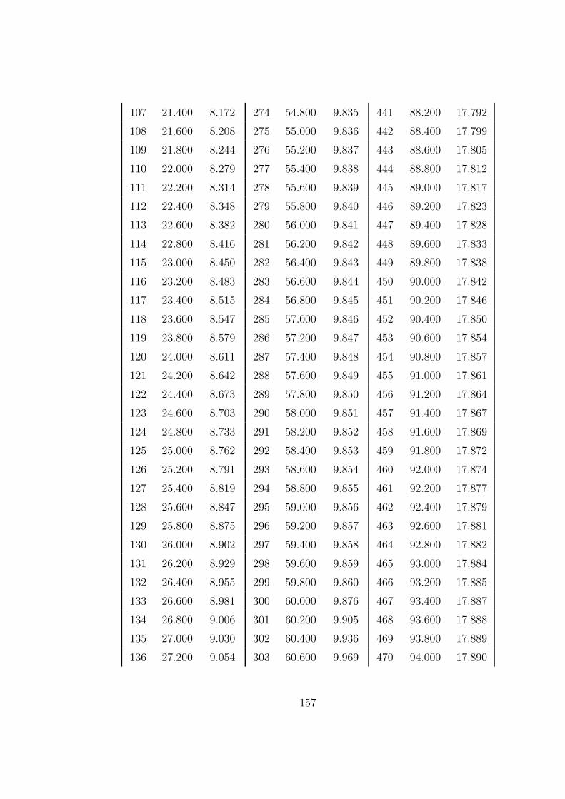
107 21.400 8.172 274 54.800 9.835 441 88.200 17.792
108 21.600 8.208 275 55.000 9.836 442 88.400 17.799
109 21.800 8.244 276 55.200 9.837 443 88.600 17.805
110 22.000 8.279 277 55.400 9.838 444 88.800 17.812
111 22.200 8.314 278 55.600 9.839 445 89.000 17.817
112 22.400 8.348 279 55.800 9.840 446 89.200 17.823
113 22.600 8.382 280 56.000 9.841 447 89.400 17.828
114 22.800 8.416 281 56.200 9.842 448 89.600 17.833
115 23.000 8.450 282 56.400 9.843 449 89.800 17.838
116 23.200 8.483 283 56.600 9.844 450 90.000 17.842
117 23.400 8.515 284 56.800 9.845 451 90.200 17.846
118 23.600 8.547 285 57.000 9.846 452 90.400 17.850
119 23.800 8.579 286 57.200 9.847 453 90.600 17.854
120 24.000 8.611 287 57.400 9.848 454 90.800 17.857
121 24.200 8.642 288 57.600 9.849 455 91.000 17.861
122 24.400 8.673 289 57.800 9.850 456 91.200 17.864
123 24.600 8.703 290 58.000 9.851 457 91.400 17.867
124 24.800 8.733 291 58.200 9.852 458 91.600 17.869
125 25.000 8.762 292 58.400 9.853 459 91.800 17.872
126 25.200 8.791 293 58.600 9.854 460 92.000 17.874
127 25.400 8.819 294 58.800 9.855 461 92.200 17.877
128 25.600 8.847 295 59.000 9.856 462 92.400 17.879
129 25.800 8.875 296 59.200 9.857 463 92.600 17.881
130 26.000 8.902 297 59.400 9.858 464 92.800 17.882
131 26.200 8.929 298 59.600 9.859 465 93.000 17.884
132 26.400 8.955 299 59.800 9.860 466 93.200 17.885
133 26.600 8.981 300 60.000 9.876 467 93.400 17.887
134 26.800 9.006 301 60.200 9.905 468 93.600 17.888
135 27.000 9.030 302 60.400 9.936 469 93.800 17.889
136 27.200 9.054 303 60.600 9.969 470 94.000 17.890
157
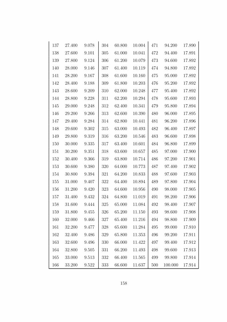
137 27.400 9.078 304 60.800 10.004 471 94.200 17.890
138 27.600 9.101 305 61.000 10.041 472 94.400 17.891
139 27.800 9.124 306 61.200 10.079 473 94.600 17.892
140 28.000 9.146 307 61.400 10.119 474 94.800 17.892
141 28.200 9.167 308 61.600 10.160 475 95.000 17.892
142 28.400 9.188 309 61.800 10.203 476 95.200 17.892
143 28.600 9.209 310 62.000 10.248 477 95.400 17.892
144 28.800 9.228 311 62.200 10.294 478 95.600 17.893
145 29.000 9.248 312 62.400 10.341 479 95.800 17.894
146 29.200 9.266 313 62.600 10.390 480 96.000 17.895
147 29.400 9.284 314 62.800 10.441 481 96.200 17.896
148 29.600 9.302 315 63.000 10.493 482 96.400 17.897
149 29.800 9.319 316 63.200 10.546 483 96.600 17.898
150 30.000 9.335 317 63.400 10.601 484 96.800 17.899
151 30.200 9.351 318 63.600 10.657 485 97.000 17.900
152 30.400 9.366 319 63.800 10.714 486 97.200 17.901
153 30.600 9.380 320 64.000 10.773 487 97.400 17.902
154 30.800 9.394 321 64.200 10.833 488 97.600 17.903
155 31.000 9.407 322 64.400 10.894 489 97.800 17.904
156 31.200 9.420 323 64.600 10.956 490 98.000 17.905
157 31.400 9.432 324 64.800 11.019 491 98.200 17.906
158 31.600 9.444 325 65.000 11.084 492 98.400 17.907
159 31.800 9.455 326 65.200 11.150 493 98.600 17.908
160 32.000 9.466 327 65.400 11.216 494 98.800 17.909
161 32.200 9.477 328 65.600 11.284 495 99.000 17.910
162 32.400 9.486 329 65.800 11.353 496 99.200 17.911
163 32.600 9.496 330 66.000 11.422 497 99.400 17.912
164 32.800 9.505 331 66.200 11.493 498 99.600 17.913
165 33.000 9.513 332 66.400 11.565 499 99.800 17.914
166 33.200 9.522 333 66.600 11.637 500 100.000 17.914
158
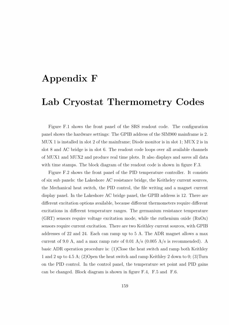
Appendix F
Lab Cryostat Thermometry Codes
Figure F.1 shows the front panel of the SRS readout code. The configuration
panel shows the hardware settings: The GPIB address of the SIM900 mainframe is 2.
MUX 1 is installed in slot 2 of the mainframe; Diode monitor is in slot 1; MUX 2 is in
slot 8 and AC bridge is in slot 6. The readout code loops over all available channels
of MUX1 and MUX2 and produce real time plots. It also displays and saves all data
with time stamps. The block diagram of the readout code is shown in figure F.3.
Figure F.2 shows the front panel of the PID temperature controller. It consists
of six sub panels: the Lakeshore AC resistance bridge, the Keitheley current sources,
the Mechanical heat switch, the PID control, the file writing and a magnet current
display panel. In the Lakeshore AC bridge panel, the GPIB address is 12. There are
different excitation options available, because different thermometers require different
excitations in different temperature ranges. The germanium resistance temperature
(GRT) sensors require voltage excitation mode, while the ruthenium oxide (RuOx)
sensors require current excitation. There are two Keithley current sources, with GPIB
addresses of 22 and 24. Each can ramp up to 5 A. The ADR magnet allows a max
current of 9.0 A, and a max ramp rate of 0.01 A/s (0.005 A/s is recommended). A
basic ADR operation procedure is: (1)Close the heat switch and ramp both Keithley
1 and 2 up to 4.5 A; (2)Open the heat switch and ramp Keithley 2 down to 0; (3)Turn
on the PID control. In the control panel, the temperature set point and PID gains
can be changed. Block diagram is shown in figure F.4, F.5 and F.6.
159
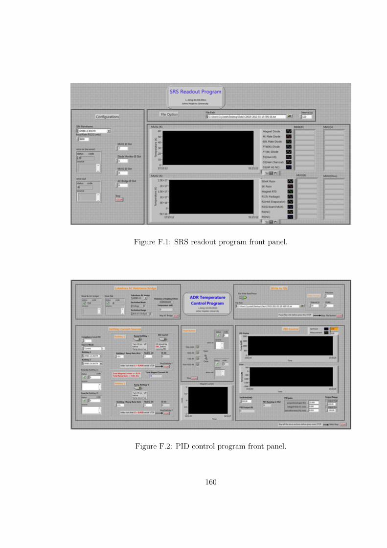
Figure F.1: SRS readout program front panel.
Figure F.2: PID control program front panel.
160
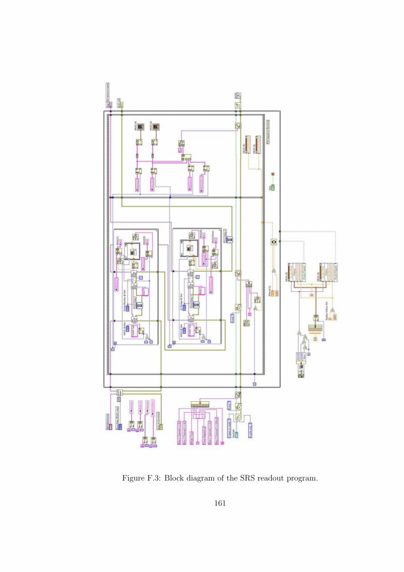
Figure F.3: Block diagram of the SRS readout program.
161
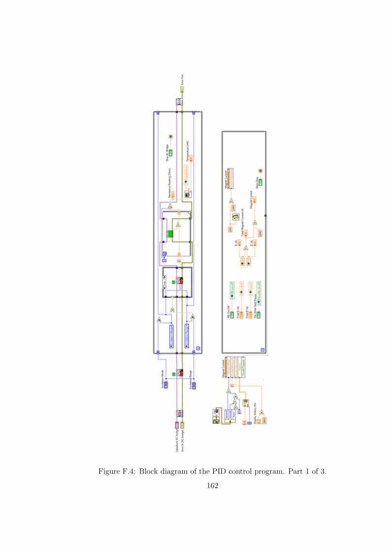
Figure F.4: Block diagram of the PID control program. Part 1 of 3.
162
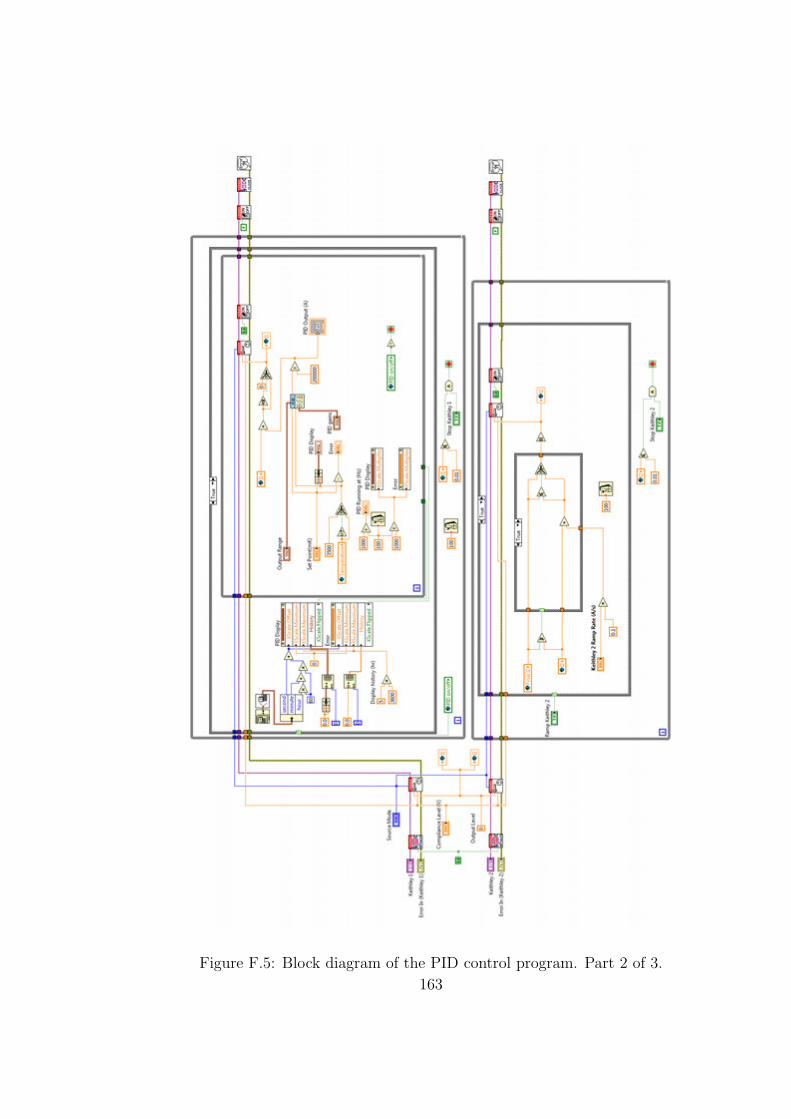
Figure F.5: Block diagram of the PID control program. Part 2 of 3.
163
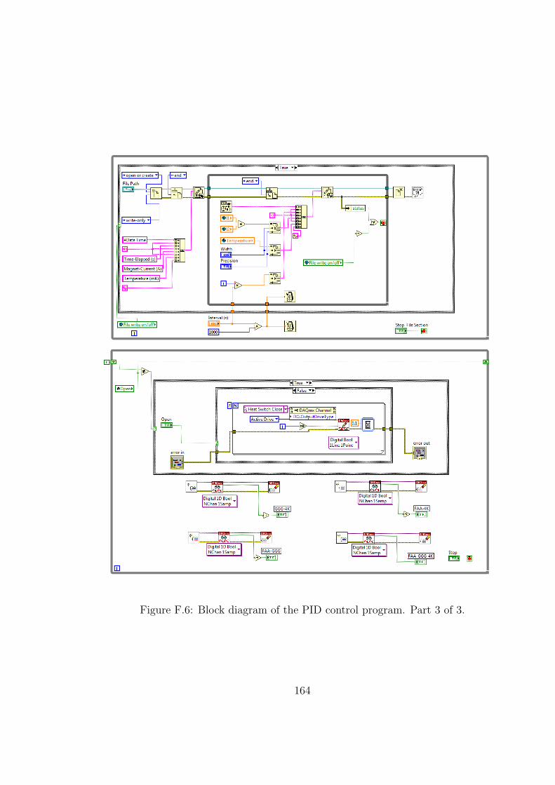
Figure F.6: Block diagram of the PID control program. Part 3 of 3.
164
Bibliography
[1] Polarization (waves). Website URLs, 2012.
http://en.wikipedia.org/wiki/Polarization_%28waves%29.
[2] C. L. Bennett, R. S. Hill, G. Hinshaw, M. R. Nolta, N. Odegard, L. Page,
D. N. Spergel, J. L. Weiland, E. L. Wright, M. Halpern, N. Jarosik, A. Kogut,
M. Limon, S. S. Meyer, G. S. Tucker, and E. Wollack. First-Year Wilkinson
Microwave Anisotropy Probe (WMAP) Observations: Foreground Emission.
Astrophys. J., Suppl. Ser., 148:97–117, September 2003.
[3] General overview of sharc-ii. Website URLs, 2004.
http://www.submm.caltech.edu/~sharc/.
[4] H. Li, C. D. Dowell, L. Kirby, G. Novak, and J. E. Vaillancourt. Design and
initial performance of SHARP, a polarimeter for the SHARC-II camera at the
Caltech Submillimeter Observatory. Applied Optics, 47:422–430, January 2008.
[5] M. S. Povich, J. M. Stone, E. Churchwell, E. G. Zweibel, M. G. Wolfire, B. L.
Babler, R. Indebetouw, M. R. Meade, and B. A. Whitney. A Multiwavelength
Study of M17: The Spectral Energy Distribution and PAH Emission Morphol-
ogy of a Massive Star Formation Region. Astrophys. J., 660:346–362, May
2007.
[6] E. W. Pellegrini, J. A. Baldwin, C. L. Brogan, M. M. Hanson, N. P. Abel, G. J.
Ferland, H. B. Nemala, G. Shaw, and T. H. Troland. A Magnetically Supported
Photodissociation Region in M17. Astrophys. J., 658:1119–1135, April 2007.
165
[7] J. L. Dotson. Polarization of the Far-Infrared Emission from M17. Astrophys.
J., 470:566, October 1996.
[8] A. Schulz, R. Lenzen, T. Schmidt, and K. Proetel. Polarization of starlight in
M 17. Astron. Astrophys., 95:94–99, February 1981.
[9] J. E. Vaillancourt. Polarized Emission from Interstellar Dust. In M.-A. Miville-
Deschenes & F. Boulanger, editor, EAS Publications Series, volume 23 of EAS
Publications Series, pages 147–164, 2007.
[10] Parameters of cosmology: What wmap records. Website URLs, 2010.
http://map.gsfc.nasa.gov/mission/sgoals_parameters_wmap.html.
[11] C. L. Bennett, M. Halpern, G. Hinshaw, N. Jarosik, A. Kogut, M. Limon,
S. S. Meyer, L. Page, D. N. Spergel, G. S. Tucker, E. Wollack, E. L. Wright,
C. Barnes, M. R. Greason, R. S. Hill, E. Komatsu, M. R. Nolta, N. Odegard,
H. V. Peiris, L. Verde, and J. L. Weiland. First-Year Wilkinson Microwave
Anisotropy Probe (WMAP) Observations: Preliminary Maps and Basic Re-
sults. Astrophys. J., Suppl. Ser., 148:1–27, September 2003.
[12] D. Larson, J. Dunkley, G. Hinshaw, E. Komatsu, M. R. Nolta, C. L. Bennett,
B. Gold, M. Halpern, R. S. Hill, N. Jarosik, A. Kogut, M. Limon, S. S. Meyer,
N. Odegard, L. Page, K. M. Smith, D. N. Spergel, G. S. Tucker, J. L. Weiland,
E. Wollack, and E. L. Wright. Seven-year Wilkinson Microwave Anisotropy
Probe (WMAP) Observations: Power Spectra and WMAP-derived Parameters.
Astrophys. J., Suppl. Ser., 192:16, February 2011.
[13] L. Page, G. Hinshaw, E. Komatsu, M. R. Nolta, D. N. Spergel, C. L. Bennett,
C. Barnes, R. Bean, O. Dore, J. Dunkley, M. Halpern, R. S. Hill, N. Jarosik,
A. Kogut, M. Limon, S. S. Meyer, N. Odegard, H. V. Peiris, G. S. Tucker,
L. Verde, J. L. Weiland, E. Wollack, and E. L. Wright. Three-Year Wilkinson
Microwave Anisotropy Probe (WMAP) Observations: Polarization Analysis.
Astrophys. J., Suppl. Ser., 170:335–376, June 2007.
166
[14] E. Komatsu, K. M. Smith, J. Dunkley, C. L. Bennett, B. Gold, G. Hinshaw,
N. Jarosik, D. Larson, M. R. Nolta, L. Page, D. N. Spergel, M. Halpern, R. S.
Hill, A. Kogut, M. Limon, S. S. Meyer, N. Odegard, G. S. Tucker, J. L. Weiland,
E. Wollack, and E. L. Wright. Seven-year Wilkinson Microwave Anisotropy
Probe (WMAP) Observations: Cosmological Interpretation. Astrophys. J.,
Suppl. Ser., 192:18, February 2011.
[15] C. L. Bennett et. al. MRI-R2: Development of a Low-Frequency Microwave
Polarimeter for Large-Scale Surveys. In A Proposal submitted to the National
Science Foundation August 2009 in response to program solicitation number
NSF 09-561, 2009.
[16] Annual variation of pwv at chajnantor. Website URLs, 2010.
http://www.apex-telescope.org/sites/chajnantor/atmosphere/pwvvar/.
[17] D. T. Chuss, E. J. Wollack, R. Henry, H. Hui, A. J. Juarez, M. Krejny, S. H.
Moseley, and G. Novak. Properties of a Variable-delay Polarization Modulator.
Applied Optics, 51(2):197–208, January 2012.
[18] G. L. James. Analysis and design of TE/11/-to-HE/11/ corrugated cylindrical
waveguide mode converters. IEEE Transactions on Microwave Theory Tech-
niques, 29:1059–1066, October 1981.
[19] D. T. Chuss, C. L. Bennett, N. Costen, E. Crowe, K. Denis, J. R. Eimer,
N. Lourie, T. A. Marriage, S. H. Moseley, K. Rostem, T. R. Stevenson,
D. Towner, K. U-Yen, G. Voellmer, E. J. Wollack, and L. Zeng. Electro-
magnetic Design of Feedhorn-Coupled Transition-Edge Sensors for Cosmic Mi-
crowave Background Polarimetry. Journal of Low Temperature Physics, page
132, November 2011.
[20] K.D. Irwin and G.C. Hilton. Transition-edge sensors. In Christian Enss, editor,
Cryogenic Particle Detection, volume 99 of Topics in Applied Physics. Springer
Berlin / Heidelberg, 2005.
167
[21] Cryostat model 104 olympus. Website URLs, 2010.
http://www.hpd-online.com/104_cryostat.php.
[22] Mce documents. Website URLs, 2012. http://e-mode.phas.ubc.ca/mcewiki/index.php/
[23] J. L. Dotson, J. Davidson, C. D. Dowell, D. A. Schleuning, and R. H. Hilde-
brand. Far-Infrared Polarimetry of Galactic Clouds from the Kuiper Airborne
Observatory. Astrophys. J., Suppl. Ser., 128:335–370, May 2000.
[24] M. Houde, P. Bastien, J. L. Dotson, C. D. Dowell, R. H. Hildebrand, R. Peng,
T. G. Phillips, J. E. Vaillancourt, and H. Yoshida. On the Measurement of
the Magnitude and Orientation of the Magnetic Field in Molecular Clouds.
Astrophys. J., 569:803–814, April 2002.
[25] G. B. Rybicki and A. P. Lightman. Radiative processes in astrophysics. New
York, Wiley-Interscience, 1979. 393 p., 1979.
[26] A. Kogut, J. Dunkley, C. L. Bennett, O. Dore, B. Gold, M. Halpern, G. Hin-
shaw, N. Jarosik, E. Komatsu, M. R. Nolta, N. Odegard, L. Page, D. N. Spergel,
G. S. Tucker, J. L. Weiland, E. Wollack, and E. L. Wright. Three-Year Wilkin-
son Microwave Anisotropy Probe (WMAP) Observations: Foreground Polar-
ization. Astrophys. J., 665:355–362, August 2007.
[27] D. P. Finkbeiner, M. Davis, and D. J. Schlegel. Extrapolation of Galactic
Dust Emission at 100 Microns to Cosmic Microwave Background Radiation
Frequencies Using FIRAS. Astrophys. J., 524:867–886, October 1999.
[28] L. Davis, Jr. and J. L. Greenstein. The Polarization of Starlight by Aligned
Dust Grains. Astrophys. J., 114:206, September 1951.
[29] D. C. B. Whittet, editor. Dust in the galactic environment, 2003.
[30] A. Lazarian. Magnetic Fields via Polarimetry: Progress of Grain Alignment
Theory. Journal of Quantitative Spectroscopy and Radiative Transfer, 79:881,
2003.
168
[31] A. Lazarian and T. Hoang. Radiative torques: analytical model and basic
properties. Mon. Not. R. Astron. Soc., 378:910–946, July 2007.
[32] W. G. Roberge. Alignment of Interstellar Dust. In A. N. Witt, G. C. Clayton, &
B. T. Draine, editor, Astrophysics of Dust, volume 309 of Astronomical Society
of the Pacific Conference Series, page 467, May 2004.
[33] E. M. Purcell. Suprathermal rotation of interstellar grains. Astrophys. J.,
231:404–416, July 1979.
[34] S. J. Barnett. Magnetization by Rotation. Physical Review, 6:239–270, October
1915.
[35] E. M. Purcell. Interstellar grains as pinwheels, pages 155–167. The Dusty
Universe, 1975.
[36] A. Z. Dolginov. Orientation of Interstellar and Interplanetary Grains. Astro-
physics and Space Science, 18:337–349, October 1972.
[37] A. Z. Dolginov and I. G. Mytrophanov. Orientation of Cosmic Dust Grains (In
Russian). Astrophysics and Space Science, 43:257, 1976.
[38] B. T. Draine and J. C. Weingartner. Radiative Torques on Interstellar Grains.
I. Superthermal Spin-up. Astrophys. J., 470:551, October 1996.
[39] B. T. Draine and J. C. Weingartner. Radiative Torques on Interstellar Grains.
II. Grain Alignment. Astrophys. J., 480:633, May 1997.
[40] A. Lazarian and B. T. Draine. Disorientation of Suprathermally Rotating
Grains and the Grain Alignment Problem. Astrophys. J., 487:248, September
1997.
[41] A. Lazarian and B. T. Draine. Thermal Flipping and Thermal Trapping: New
Elements in Grain Dynamics. Astrophys. J., Lett., 516:L37–L40, May 1999.
[42] A. Lazarian and B. T. Draine. Nuclear Spin Relaxation within Interstellar
Grains. Astrophys. J., Lett., 520:L67–L70, July 1999.
169
[43] T. Gold. The alignment of galactic dust. Mon. Not. R. Astron. Soc., 112:215,
1952.
[44] J. Cho and A. Lazarian. Grain Alignment by Radiation in Dark Clouds and
Cores. Astrophys. J., 631:361–370, September 2005.
[45] C. Heiles. 9286 Stars: An Agglomeration of Stellar Polarization Catalogs. As-
tron. J., 119:923–927, February 2000.
[46] A. Berdyugin, V. Piirola, and P. Teerikorpi. Interstellar polarization at high
galactic latitudes from distant stars. VII. A complete map for southern latitudes
b < −70. Astron. Astrophys., 424:873–876, September 2004.
[47] A. A. Goodman, T. J. Jones, E. A. Lada, and P. C. Myers. Does Near-Infrared
Polarimetry Reveal the Magnetic Field in Cold Dark Clouds? Astrophys. J.,
448:748, August 1995.
[48] H. G. Arce, A. A. Goodman, P. Bastien, N. Manset, and M. Sumner. The
Polarizing Power of the Interstellar Medium in Taurus. Astrophys. J., Lett.,
499:L93, May 1998.
[49] W. A. Hiltner. Polarization of Light from Distant Stars by Interstellar Medium.
Science, 109:165–+, February 1949.
[50] J. S. Hall. Observations of the Polarized Light from Stars. Science, 109:166–167,
February 1949.
[51] P. Fosalba, A. Lazarian, S. Prunet, and J. A. Tauber. Statistical Properties of
Galactic Starlight Polarization. Astrophys. J., 564:762–772, January 2002.
[52] B. Keating, P. Timbie, A. Polnarev, and J. Steinberger. Large Angular Scale
Polarization of the Cosmic Microwave Background Radiation and the Feasibility
of Its Detection. Astrophys. J., 495:580, March 1998.
170
[53] A. Kogut, A. J. Banday, C. L. Bennett, K. M. Gorski, G. Hinshaw, and W. T.
Reach. High-Latitude Galactic Emission in the COBE Differential Microwave
Radiometer 2 Year Sky Maps. Astrophys. J., 460:1, March 1996.
[54] A. de Oliveira-Costa, A. Kogut, M. J. Devlin, C. B. Netterfield, L. A. Page,
and E. J. Wollack. Galactic Microwave Emission at Degree Angular Scales.
Astrophys. J., Lett., 482:L17, June 1997.
[55] E. M. Leitch, A. C. S. Readhead, T. J. Pearson, and S. T. Myers. An Anomalous
Component of Galactic Emission. Astrophys. J., Lett., 486:L23, September
1997.
[56] S. R. Hildebrandt, R. Rebolo, J. A. Rubino-Martın, R. A. Watson, C. M.
Gutierrez, R. J. Hoyland, and E. S. Battistelli. COSMOSOMAS observations
of the cosmic microwave background and Galactic foregrounds at 11 GHz: evi-
dence for anomalous microwave emission at high Galactic latitude. Mon. Not.
R. Astron. Soc., 382:594–608, December 2007.
[57] D. P. Finkbeiner. Microwave Interstellar Medium Emission Observed by the
Wilkinson Microwave Anisotropy Probe. Astrophys. J., 614:186–193, October
2004.
[58] R. A. Watson, R. Rebolo, J. A. Rubino-Martın, S. Hildebrandt, C. M. Gutierrez,
S. Fernandez-Cerezo, R. J. Hoyland, and E. S. Battistelli. Detection of Anoma-
lous Microwave Emission in the Perseus Molecular Cloud with the COSMOSO-
MAS Experiment. Astrophys. J., Lett., 624:L89–L92, May 2005.
[59] R. D. Davies, C. Dickinson, A. J. Banday, T. R. Jaffe, K. M. Gorski, and
R. J. Davis. A determination of the spectra of Galactic components observed
by the Wilkinson Microwave Anisotropy Probe. Mon. Not. R. Astron. Soc.,
370:1125–1139, August 2006.
[60] G. Dobler, B. Draine, and D. P. Finkbeiner. Constraining Spinning Dust Pa-
rameters with the WMAP Five-Year Data. Astrophys. J., 699:1374–1388, July
2009.
171
[61] G. Dobler and D. P. Finkbeiner. Extended Anomalous Foreground Emission in
the WMAP Three-Year Data. Astrophys. J., 680:1222–1234, June 2008.
[62] B. T. Draine and A. Lazarian. Diffuse Galactic Emission from Spinning Dust
Grains. Astrophys. J., Lett., 494:L19, February 1998.
[63] B. T. Draine and A. Lazarian. Electric Dipole Radiation from Spinning Dust
Grains. Astrophys. J., 508:157–179, November 1998.
[64] Y. Ali-Haımoud, C. M. Hirata, and C. Dickinson. A refined model for spinning
dust radiation. Mon. Not. R. Astron. Soc., 395:1055–1078, May 2009.
[65] B. T. Draine and A. Lazarian. Magnetic Dipole Microwave Emission from Dust
Grains. Astrophys. J., 512:740–754, February 1999.
[66] A. de Oliveira-Costa, M. Tegmark, D. P. Finkbeiner, R. D. Davies, C. M.
Gutierrez, L. M. Haffner, A. W. Jones, A. N. Lasenby, R. Rebolo, R. J.
Reynolds, S. L. Tufte, and R. A. Watson. A New Spin on Galactic Dust.
Astrophys. J., 567:363–369, March 2002.
[67] S. Casassus, G. F. Cabrera, F. Forster, T. J. Pearson, A. C. S. Readhead, and
C. Dickinson. Morphological Analysis of the Centimeter-Wave Continuum in
the Dark Cloud LDN 1622. Astrophys. J., 639:951–964, March 2006.
[68] B. D. Savage and K. R. Sembach. Interstellar Abundances from Absorption-Line
Observations with the Hubble Space Telescope. Ann. Rev. Astron. Astrophys.,
34:279–330, 1996.
[69] K. R. Sembach and B. D. Savage. The Gas and Dust Abundances of Diffuse
Halo Clouds in the Milky Way. Astrophys. J., 457:211, January 1996.
[70] A. Lazarian and B. T. Draine. Resonance Paramagnetic Relaxation and Align-
ment of Small Grains. Astrophys. J., Lett., 536:L15–L18, June 2000.
172
[71] D. C. B. Whittet. Polarization of Starlight. In A. N. Witt, G. C. Clayton, &
B. T. Draine, editor, Astrophysics of Dust, volume 309 of Astronomical Society
of the Pacific Conference Series, page 65, May 2004.
[72] P. G. Martin. On Predicting the Polarization of Low Frequency Emission by
Diffuse Interstellar Dust. In M.-A. Miville-Deschenes & F. Boulanger, editor,
EAS Publications Series, volume 23 of EAS Publications Series, pages 165–188,
2007.
[73] D. K. Aitken, C. H. Smith, T. J. T. Moore, and P. F. Roche. Mid-infrared
polarization studies of SgrA: a three-dimensional study of the central parsec.
Mon. Not. R. Astron. Soc., 299:743–752, September 1998.
[74] A. G. G. M. Tielens. The Physics and Chemistry of the Interstellar Medium.
September 2005.
[75] R. M. Crutcher. Magnetic Fields in Molecular Clouds: Observations Confront
Theory. Astrophys. J., 520:706–713, August 1999.
[76] L. Mestel and P. A. Strittmatter. The magnetic field of a contracting gas cloud-
II. Finite diffusion effects-an illustrative example. Mon. Not. R. Astron. Soc.,
137:95, 1967.
[77] W. Cudlip, I. Furniss, K. J. King, and R. E. Jennings. Far infrared polarimetry
of W51A and M42. Mon. Not. R. Astron. Soc., 200:1169–1173, September 1982.
[78] R. H. Hildebrand, M. Dragovan, and G. Novak. Detection of submillimeter
polarization in the Orion nebula. Astrophys. J., Lett, 284:L51–L54, September
1984.
[79] S. R. Platt, R. H. Hildebrand, R. J. Pernic, J. A. Davidson, and G. Novak.
100-micron array polarimetry from the Kuiper Airborne Observatory - Instru-
mentation, techniques, and first results. Publ. Astron. Soc. Pac., 103:1193–1210,
November 1991.
173
[80] B. C. Matthews, C. A. McPhee, L. M. Fissel, and R. L. Curran. The Legacy
of SCUPOL: 850 µm Imaging Polarimetry from 1997 to 2005. Astrophys. J.,
Suppl. Ser., 182:143–204, May 2009.
[81] B. C. Matthews, C. A. McPhee, L. M. Fissel, and R. L. Curran. SCUPOL
Legacy polarimetry of SCUBA (Matthews+, 2009). VizieR Online Data Cata-
log, 218:20143, January 2010.
[82] D. A. Schleuning, C. D. Dowell, R. H. Hildebrand, S. R. Platt, and G. Novak.
HERTZ, A Submillimeter Polarimeter. Publ. Astron. Soc. Pac., 109:307–318,
March 1997.
[83] G. Novak, D. T. Chuss, J. A. Davidson, J. L. Dotson, C. D. Dowell, R. H.
Hildebrand, M. Houde, L. Kirby, M. Krejny, A. Lazarian, H.-b. Li, S. H.
Moseley, J. E. Vaillancourt, and F. Yusef-Zadeh. A polarimetry module for
CSO/SHARC-II. In C. M. Bradford, P. A. R. Ade, J. E. Aguirre, J. J. Bock,
M. Dragovan, L. Duband, L. Earle, J. Glenn, H. Matsuhara, B. J. Naylor,
H. T. Nguyen, M. Yun, & J. Zmuidzinas, editor, Society of Photo-Optical In-
strumentation Engineers (SPIE) Conference Series, volume 5498 of Society of
Photo-Optical Instrumentation Engineers (SPIE) Conference Series, pages 278–
289, October 2004.
[84] T.G. Phillips. The caltech submillimeter observatory. InMicrowave Symposium,
2007. IEEE/MTT-S International, pages 1849 –1852, june 2007.
[85] M. Leong, R. Peng, M. Houde, H. Yoshida, R. Chamberlin, and T. G. Phillips.
A CSO submillimeter active optics system. In Society of Photo-Optical In-
strumentation Engineers (SPIE) Conference Series, volume 6275 of Society of
Photo-Optical Instrumentation Engineers (SPIE) Conference Series, July 2006.
[86] T. G. Phillips and D. P. Woody. Millimeter- and submillimeter-wave receivers.
Ann. Rev. Astron. Astrophys., 20:285–321, 1982.
[87] J. W. Kooi, R. A. Chamberlin, R. Monje, B. Force, D. Miller, and T. G. Phillips.
174
Technology Development for the Caltech Submillimeter Observatory Balanced
Receivers. ArXiv e-prints, January 2012.
[88] C. D. Dowell, C. A. Allen, R. S. Babu, M. M. Freund, M. Gardner, J. Groseth,
M. D. Jhabvala, A. Kovacs, D. C. Lis, S. H. Moseley, Jr., T. G. Phillips, R. F.
Silverberg, G. M. Voellmer, and H. Yoshida. SHARC II: a Caltech submillimeter
observatory facility camera with 384 pixels. In T. G. Phillips and J. Zmuidzi-
nas, editors, Society of Photo-Optical Instrumentation Engineers (SPIE) Con-
ference Series, volume 4855 of Society of Photo-Optical Instrumentation Engi-
neers (SPIE) Conference Series, pages 73–87, February 2003.
[89] Sharp - the sharc ii polarimeter. Website URLs, 2012.
http://lennon.astro.northwestern.edu/SHARP/instrument.html.
[90] E. Pascale, P. A. R. Ade, J. J. Bock, E. L. Chapin, J. Chung, M. J. Devlin,
S. Dicker, M. Griffin, J. O. Gundersen, M. Halpern, P. C. Hargrave, D. H.
Hughes, J. Klein, C. J. MacTavish, G. Marsden, P. G. Martin, T. G. Martin,
P. Mauskopf, C. B. Netterfield, L. Olmi, G. Patanchon, M. Rex, D. Scott,
C. Semisch, N. Thomas, M. D. P. Truch, C. Tucker, G. S. Tucker, M. P. Viero,
and D. V. Wiebe. The Balloon-borne Large Aperture Submillimeter Telescope:
BLAST. Astrophys. J., 681:400–414, July 2008.
[91] W. Holland, M. MacIntosh, A. Fairley, D. Kelly, D. Montgomery, D. Go-
stick, E. Atad-Ettedgui, M. Ellis, I. Robson, M. Hollister, A. Woodcraft,
P. Ade, I. Walker, K. Irwin, G. Hilton, W. Duncan, C. Reintsema, A. Wal-
ton, W. Parkes, C. Dunare, M. Fich, J. Kycia, M. Halpern, D. Scott, A. Gibb,
J. Molnar, E. Chapin, D. Bintley, S. Craig, T. Chylek, T. Jenness, F. Economou,
and G. Davis. SCUBA-2: a 10,000-pixel submillimeter camera for the James
Clerk Maxwell Telescope. In Society of Photo-Optical Instrumentation Engi-
neers (SPIE) Conference Series, volume 6275 of Society of Photo-Optical In-
strumentation Engineers (SPIE) Conference Series, July 2006.
175
[92] M. Nielbock, R. Chini, M. Jutte, and E. Manthey. High mass Class I sources
in M 17. Astron. Astrophys., 377:273–284, October 2001.
[93] B. C. Dunne, Y.-H. Chu, C.-H. R. Chen, J. D. Lowry, L. Townsley, R. A.
Gruendl, M. A. Guerrero, and M. Rosado. Diffuse X-Ray Emission from the
Quiescent Superbubble M17, the Omega Nebula. Astrophys. J., 590:306–313,
June 2003.
[94] L. K. Townsley, E. D. Feigelson, T. Montmerle, P. S. Broos, Y.-H. Chu, and
G. P. Garmire. 10 MK Gas in M17 and the Rosette Nebula: X-Ray Flows in
Galactic H II Regions. Astrophys. J., 593:874–905, August 2003.
[95] V. A. Gagen-Torn and N. V. Voshchinnikov. Polarization study of the nebula
NGC 6618 and neighboring stars. Astrofizika, 13:569–586, November 1977.
[96] R. H. Hildebrand. Magnetic fields and stardust. Quarterly Journal of the RAS,
29:327–351, September 1988.
[97] R. H. Hildebrand, J. L. Dotson, C. D. Dowell, D. A. Schleuning, and J. E. Vail-
lancourt. The Far-Infrared Polarization Spectrum: First Results and Analysis.
Astrophys. J., 516:834–842, May 1999.
[98] J. E. Vaillancourt. Analysis of the Far-Infrared/Submillimeter Polarization
Spectrum Based on Temperature Maps of Orion. Astrophys. J., Suppl. Ser.,
142:53–69, September 2002.
[99] R. Hildebrand and L. Kirby. Polarization of FIR/Sub-mm Dust Emission. In
A. N. Witt, G. C. Clayton, and B. T. Draine, editors, Astrophysics of Dust,
volume 309 of Astronomical Society of the Pacific Conference Series, page 515,
May 2004.
[100] J. E. Vaillancourt, C. D. Dowell, R. H. Hildebrand, L. Kirby, M. M. Krejny,
H.-b. Li, G. Novak, M. Houde, H. Shinnaga, and M. Attard. New Results on the
Submillimeter Polarization Spectrum of the Orion Molecular Cloud. Astrophys.
J., Lett., 679:L25–L28, May 2008.
176
[101] T. J. Bethell, A. Chepurnov, A. Lazarian, and J. Kim. Polarization of Dust
Emission in Clumpy Molecular Clouds and Cores. Astrophys. J., 663:1055–1068,
July 2007.
[102] B. T. Draine and A. A. Fraisse. Polarized Far-Infrared and Submillimeter Emis-
sion from Interstellar Dust. Astrophys. J., 696:1–11, May 2009.
[103] E. Hubble. A Relation between Distance and Radial Velocity among Extra-
Galactic Nebulae. Proceedings of the National Academy of Science, 15:168–173,
March 1929.
[104] R. A. Alpher, H. Bethe, and G. Gamow. The Origin of Chemical Elements.
Physical Review, 73:803–804, April 1948.
[105] R. A. Alpher and R. C. Herman. On the Relative Abundance of the Elements.
Physical Review, 74:1737–1742, December 1948.
[106] M. Fumagalli, J. M. O’Meara, and J. X. Prochaska. Detection of Pristine Gas
Two Billion Years After the Big Bang. Science, 334:1245–, December 2011.
[107] F. Hoyle. A New Model for the Expanding Universe. Mon. Not. R. Astron.
Soc., 108:372, 1948.
[108] A. A. Penzias and R. W. Wilson. A Measurement of Excess Antenna Temper-
ature at 4080 Mc/s. Astrophys. J., 142:419–421, July 1965.
[109] N. W. Boggess, J. C. Mather, R. Weiss, C. L. Bennett, E. S. Cheng, E. Dwek,
S. Gulkis, M. G. Hauser, M. A. Janssen, T. Kelsall, S. S. Meyer, S. H. Moseley,
T. L. Murdock, R. A. Shafer, R. F. Silverberg, G. F. Smoot, D. T. Wilkinson,
and E. L. Wright. The COBE mission - Its design and performance two years
after launch. Astrophys. J., 397:420–429, October 1992.
[110] E. Bertschinger. Simulations of Structure Formation in the Universe. Ann. Rev.
Astron. Astrophys., 36:599–654, 1998.
177
[111] A. H. Guth and S.-H. H. Tye. Phase Transitions and Magnetic Monopole
Production in the Very Early Universe. Physical Review Letters, 44:963, April
1980.
[112] A. H. Guth. Inflationary universe: A possible solution to the horizon and
flatness problems. Phys. Rev. D, 23:347–356, January 1981.
[113] A. A. Starobinsky. A new type of isotropic cosmological models without singu-
larity. Physics Letters B, 91:99–102, March 1980.
[114] A. D. Linde. A new inflationary universe scenario: A possible solution of the
horizon, flatness, homogeneity, isotropy and primordial monopole problems.
Physics Letters B, 108:389–393, February 1982.
[115] A. Albrecht and P. J. Steinhardt. Cosmology for grand unified theories with
radiatively induced symmetry breaking. Physical Review Letters, 48:1220–1223,
April 1982.
[116] C. L. Chang. The Cryogenic Dark Matter Search (CDMS-II) experiment: First
results from the Soudan Mine. PhD thesis, Stanford University, California,
USA, 2005.
[117] A. Hime. SNOLAB - An International Facility for Underground Science. In
B. Cleveland, R. Ford, & M. Chen, editor, Topical Workshop on Low Radioac-
tivity Techniques: LRT 2004., volume 785 of American Institute of Physics
Conference Series, pages 27–36, September 2005.
[118] P. Picchi and F. Pietropaolo. Physics projects for a future CERN-LNGS neu-
trino programme. Nuclear Physics B Proceedings Supplements, 77:187–197, May
1999.
[119] A. S. Murphy and Uk Dark Matter Collaboration. The Boulby Underground
Laboratory. In N. J. C. Spooner & V. Kudryavtsev, editor, The Identification
of Dark Matter, pages 453–459, April 2005.
178
[120] Lbne/Dusel Collaborations and C. Mariani. DUSEL (Deep Underground Sci-
ence and Engineering Laboratory) and LBNE (Long Baseline Neutrino Experi-
ment). Nuclear Physics B Proceedings Supplements, 217:344–346, August 2011.
[121] A. G. Riess, A. V. Filippenko, P. Challis, A. Clocchiatti, A. Diercks, P. M.
Garnavich, R. L. Gilliland, C. J. Hogan, S. Jha, R. P. Kirshner, B. Leibundgut,
M. M. Phillips, D. Reiss, B. P. Schmidt, R. A. Schommer, R. C. Smith, J. Spy-
romilio, C. Stubbs, N. B. Suntzeff, and J. Tonry. Observational Evidence from
Supernovae for an Accelerating Universe and a Cosmological Constant. Astron.
J., 116:1009–1038, September 1998.
[122] R. G. Crittenden and N. Turok. Looking for a Cosmological Constant with the
Rees-Sciama Effect. Physical Review Letters, 76:575–578, January 1996.
[123] S. Ho, C. Hirata, N. Padmanabhan, U. Seljak, and N. Bahcall. Correlation
of CMB with large-scale structure. I. Integrated Sachs-Wolfe tomography and
cosmological implications. Phys. Rev. D, 78(4):043519, August 2008.
[124] T. Giannantonio, R. Scranton, R. G. Crittenden, R. C. Nichol, S. P. Boughn,
A. D. Myers, and G. T. Richards. Combined analysis of the integrated Sachs-
Wolfe effect and cosmological implications. Phys. Rev. D, 77(12):123520, June
2008.
[125] J. H. Goldstein, P. A. R. Ade, J. J. Bock, J. R. Bond, C. Cantalupo, C. R.
Contaldi, M. D. Daub, W. L. Holzapfel, C. Kuo, A. E. Lange, M. Lueker,
M. Newcomb, J. B. Peterson, D. Pogosyan, J. E. Ruhl, M. C. Runyan, and
E. Torbet. Estimates of Cosmological Parameters Using the Cosmic Microwave
Background Angular Power Spectrum of ACBAR. Astrophys. J., 599:773–785,
December 2003.
[126] J. W. Fowler, V. Acquaviva, P. A. R. Ade, P. Aguirre, M. Amiri, J. W. Ap-
pel, L. F. Barrientos, E. S. Battistelli, J. R. Bond, B. Brown, B. Burger,
J. Chervenak, S. Das, M. J. Devlin, S. R. Dicker, W. B. Doriese, J. Dunkley,
179
R. Dunner, T. Essinger-Hileman, R. P. Fisher, A. Hajian, M. Halpern, M. Has-
selfield, C. Hernandez-Monteagudo, G. C. Hilton, M. Hilton, A. D. Hincks,
R. Hlozek, K. M. Huffenberger, D. H. Hughes, J. P. Hughes, L. Infante, K. D.
Irwin, R. Jimenez, J. B. Juin, M. Kaul, J. Klein, A. Kosowsky, J. M. Lau,
M. Limon, Y.-T. Lin, R. H. Lupton, T. A. Marriage, D. Marsden, K. Mar-
tocci, P. Mauskopf, F. Menanteau, K. Moodley, H. Moseley, C. B. Netterfield,
M. D. Niemack, M. R. Nolta, L. A. Page, L. Parker, B. Partridge, H. Quintana,
B. Reid, N. Sehgal, J. Sievers, D. N. Spergel, S. T. Staggs, D. S. Swetz, E. R.
Switzer, R. Thornton, H. Trac, C. Tucker, L. Verde, R. Warne, G. Wilson,
E. Wollack, and Y. Zhao. The Atacama Cosmology Telescope: A Measurement
of the 600 < ℓ < 8000 Cosmic Microwave Background Power Spectrum at 148
GHz. Astrophys. J., 722:1148–1161, October 2010.
[127] S. Das, T. A. Marriage, P. A. R. Ade, P. Aguirre, M. Amiri, J. W. Appel,
L. F. Barrientos, E. S. Battistelli, J. R. Bond, B. Brown, B. Burger, J. Cherve-
nak, M. J. Devlin, S. R. Dicker, W. Bertrand Doriese, J. Dunkley, R. Dunner,
T. Essinger-Hileman, R. P. Fisher, J. W. Fowler, A. Hajian, M. Halpern,
M. Hasselfield, C. Hernandez-Monteagudo, G. C. Hilton, M. Hilton, A. D.
Hincks, R. Hlozek, K. M. Huffenberger, D. H. Hughes, J. P. Hughes, L. Infante,
K. D. Irwin, J. Baptiste Juin, M. Kaul, J. Klein, A. Kosowsky, J. M. Lau,
M. Limon, Y.-T. Lin, R. H. Lupton, D. Marsden, K. Martocci, P. Mauskopf,
F. Menanteau, K. Moodley, H. Moseley, C. B. Netterfield, M. D. Niemack, M. R.
Nolta, L. A. Page, L. Parker, B. Partridge, B. Reid, N. Sehgal, B. D. Sherwin,
J. Sievers, D. N. Spergel, S. T. Staggs, D. S. Swetz, E. R. Switzer, R. Thornton,
H. Trac, C. Tucker, R. Warne, E. Wollack, and Y. Zhao. The Atacama Cosmol-
ogy Telescope: A Measurement of the Cosmic Microwave Background Power
Spectrum at 148 and 218 GHz from the 2008 Southern Survey. Astrophys. J.,
729:62, March 2011.
[128] R. Keisler, C. L. Reichardt, K. A. Aird, B. A. Benson, L. E. Bleem, J. E.
Carlstrom, C. L. Chang, H. M. Cho, T. M. Crawford, A. T. Crites, T. de
Haan, M. A. Dobbs, J. Dudley, E. M. George, N. W. Halverson, G. P. Holder,
180
W. L. Holzapfel, S. Hoover, Z. Hou, J. D. Hrubes, M. Joy, L. Knox, A. T.
Lee, E. M. Leitch, M. Lueker, D. Luong-Van, J. J. McMahon, J. Mehl, S. S.
Meyer, M. Millea, J. J. Mohr, T. E. Montroy, T. Natoli, S. Padin, T. Plagge,
C. Pryke, J. E. Ruhl, K. K. Schaffer, L. Shaw, E. Shirokoff, H. G. Spieler,
Z. Staniszewski, A. A. Stark, K. Story, A. van Engelen, K. Vanderlinde, J. D.
Vieira, R. Williamson, and O. Zahn. A Measurement of the Damping Tail of the
Cosmic Microwave Background Power Spectrum with the South Pole Telescope.
Astrophys. J., 743:28, December 2011.
[129] M. Kamionkowski, A. Kosowsky, and A. Stebbins. A Probe of Primordial
Gravity Waves and Vorticity. Physical Review Letters, 78:2058–2061, March
1997.
[130] J. M. Kovac, E. M. Leitch, C. Pryke, J. E. Carlstrom, N. W. Halverson, and
W. L. Holzapfel. Detection of polarization in the cosmic microwave background
using DASI. Nature, 420:772–787, December 2002.
[131] QUIET Collaboration, C. Bischoff, A. Brizius, I. Buder, Y. Chinone, K. Cleary,
R. N. Dumoulin, A. Kusaka, R. Monsalve, S. K. Næss, L. B. Newburgh,
R. Reeves, K. M. Smith, I. K. Wehus, J. A. Zuntz, J. T. L. Zwart, L. Bronf-
man, R. Bustos, S. E. Church, C. Dickinson, H. K. Eriksen, P. G. Ferreira,
T. Gaier, J. O. Gundersen, M. Hasegawa, M. Hazumi, K. M. Huffenberger,
M. E. Jones, P. Kangaslahti, D. J. Kapner, C. R. Lawrence, M. Limon, J. May,
J. J. McMahon, A. D. Miller, H. Nguyen, G. W. Nixon, T. J. Pearson, L. Pic-
cirillo, S. J. E. Radford, A. C. S. Readhead, J. L. Richards, D. Samtleben,
M. Seiffert, M. C. Shepherd, S. T. Staggs, O. Tajima, K. L. Thompson, K. Van-
derlinde, R. Williamson, and B. Winstein. First Season QUIET Observations:
Measurements of Cosmic Microwave Background Polarization Power Spectra at
43 GHz in the Multipole Range 25 ≤ ℓ ≤ 475. Astrophys. J., 741:111, November
2011.
[132] S. M. Leach, A. R. Liddle, J. Martin, and D. J. Schwarz. Cosmological parame-
181
ter estimation and the inflationary cosmology. Phys. Rev. D, 66(2):023515, July
2002.
[133] H. V. Peiris, E. Komatsu, L. Verde, D. N. Spergel, C. L. Bennett, M. Halpern,
G. Hinshaw, N. Jarosik, A. Kogut, M. Limon, S. S. Meyer, L. Page, G. S. Tucker,
E. Wollack, and E. L. Wright. First-Year Wilkinson Microwave Anisotropy
Probe (WMAP) Observations: Implications For Inflation. Astrophys. J., Suppl.
Ser., 148:213–231, September 2003.
[134] V. A. Rubakov, M. V. Sazhin, and A. V. Veryaskin. Graviton creation in
the inflationary universe and the grand unification scale. Physics Letters B,
115:189–192, September 1982.
[135] Y. Zhao, C. Allen, M. Amiri, J. W. Appel, E. S. Battistelli, B. Burger, J. A.
Chervenak, A. J. Dahlen, S. Denny, M. J. Devlin, S. R. Dicker, W. B. Doriese,
R. Dunner, T. Essinger-Hileman, R. P. Fisher, J. W. Fowler, M. Halpern, G. C.
Hilton, A. D. Hincks, K. D. Irwin, N. Jarosik, J. Klein, J. M. Lau, T. A. Mar-
riage, K. L. Martocci, S. H. Moseley, M. D. Niemack, L. Page, L. P. Parker,
A. Sederberg, S. T. Staggs, O. R. Stryzak, D. S. Swetz, E. R. Switzer, R. J.
Thornton, and E. J. Wollack. Characterization of transition edge sensors for
the Millimeter Bolometer Array Camera on the Atacama Cosmology Telescope.
In Society of Photo-Optical Instrumentation Engineers (SPIE) Conference Se-
ries, volume 7020 of Society of Photo-Optical Instrumentation Engineers (SPIE)
Conference Series, August 2008.
[136] M. Kamionkowski, A. Kosowsky, and A. Stebbins. Statistics of cosmic mi-
crowave background polarization. Phys. Rev. D, 55:7368–7388, June 1997.
[137] J. Lazear, D. Benford, D. Chuss, D. Fixsen, J. Hinderks, G. Hinshaw, C. Jhab-
vala, B. Johnson, A. Kogut, P. Mirel, H. Mosely, J. Staghun, E. Wollack, A. We-
ston, K. Vlahacos, C. Bennett, J. Eimer, M. Halpern, K. Irwin, J. Dotson,
P. Ade, and C. Tucker. PIPER: Primordial Inflation Polarization Explorer. In
American Astronomical Society Meeting Abstracts 218, page 233.01, May 2011.
182
[138] T. E. Montroy, P. A. R. Ade, R. Bihary, J. J. Bock, J. R. Bond, J. Brevick,
C. R. Contaldi, B. P. Crill, A. Crites, O. Dore, L. Duband, S. R. Golwala,
M. Halpern, G. Hilton, W. Holmes, V. V. Hristov, K. Irwin, W. C. Jones, C. L.
Kuo, A. E. Lange, C. J. MacTavish, P. Mason, J. Mulder, C. B. Netterfield,
E. Pascale, J. E. Ruhl, A. Trangsrud, C. Tucker, A. Turner, and M. Viero. SPI-
DER: a new balloon-borne experiment to measure CMB polarization on large
angular scales. In Society of Photo-Optical Instrumentation Engineers (SPIE)
Conference Series, volume 6267 of Society of Photo-Optical Instrumentation
Engineers (SPIE) Conference Series, July 2006.
[139] P. Oxley, P. A. Ade, C. Baccigalupi, P. deBernardis, H.-M. Cho, M. J. De-
vlin, S. Hanany, B. R. Johnson, T. Jones, A. T. Lee, T. Matsumura, A. D.
Miller, M. Milligan, T. Renbarger, H. G. Spieler, R. Stompor, G. S. Tucker,
and M. Zaldarriaga. The EBEX experiment. In M. Strojnik, editor, Society
of Photo-Optical Instrumentation Engineers (SPIE) Conference Series, volume
5543 of Society of Photo-Optical Instrumentation Engineers (SPIE) Conference
Series, pages 320–331, November 2004.
[140] P. L. Richards. Bolometers for infrared and millimeter waves. Journal of Applied
Physics, 76:1–24, July 1994.
[141] M. Bowden, A. N. Taylor, K. M. Ganga, P. A. R. Ade, J. J. Bock, G. Cahill,
J. E. Carlstrom, S. E. Church, W. K. Gear, J. R. Hinderks, W. Hu, B. G.
Keating, J. Kovac, A. E. Lange, E. M. Leitch, B. Maffei, O. E. Mallie, S. J.
Melhuish, J. A. Murphy, G. Pisano, L. Piccirillo, C. Pryke, B. A. Rusholme,
C. O’Sullivan, and K. Thompson. Scientific optimization of a ground-based
CMB polarization experiment. Mon. Not. R. Astron. Soc., 349:321–335, March
2004.
[142] D. Larson. Private Communication, 2010.
[143] S. Dodelson. Modern cosmology. Academic Press. ISBN 0-12-219141-2, 2003,
XIII + 440 p., 2003.
183

[144] J. R. Pardo, J. Cernicharo, and E. Serabyn. Atmospheric transmission at mi-
crowaves (ATM): an improved model for millimeter/submillimeter applications.
IEEE Transactions on Antennas and Propagation, 49:1683–1694, December
2001.
[145] H. J. Liebe. MPM - An atmospheric millimeter-wave propagation model. In-
ternational Journal of Infrared and Millimeter Waves, 10:631–650, June 1989.
[146] J. R. Pardo, M. C. Wiedner, E. Serabyn, C. D. Wilson, C. Cunningham, R. E.
Hills, and J. Cernicharo. Side-by-Side Comparison of Fourier Transform Spec-
troscopy and Water Vapor Radiometry as Tools for the Calibration of Mil-
limeter/Submillimeter Ground-based Observatories. Astrophys. J., Suppl. Ser.,
153:363–367, July 2004.
[147] J. C. Mather. Bolometer noise: nonequilibrium thoery. Applied Optics, 21:1125–
1129, March 1982.
[148] D. T. Chuss, P. A. R. Ade, D. J. Benford, C. L. Bennett, J. L. Dotson, J. R.
Eimer, D. J. Fixsen, M. Halpern, G. Hilton, J. Hinderks, G. Hinshaw, K. Irwin,
M. L. Jackson, M. A. Jah, N. Jethava, C. Jhabvala, A. J. Kogut, L. Lowe,
N. McCullagh, T. Miller, P. Mirel, S. H. Moseley, S. Rodriguez, K. Rostem,
E. Sharp, J. G. Staguhn, C. E. Tucker, G. M. Voellmer, E. J. Wollack, and
L. Zeng. The Primordial Inflation Polarization Explorer (PIPER). In Society
of Photo-Optical Instrumentation Engineers (SPIE) Conference Series, volume
7741 of Society of Photo-Optical Instrumentation Engineers (SPIE) Conference
Series, July 2010.
[149] M. Krejny, D. Chuss, C. D. D’Aubigny, D. Golish, M. Houde, H. Hui, C. Kulesa,
R. F. Loewenstein, S. H. Moseley, G. Novak, G. Voellmer, C. Walker, and
E. Wollack. The Hertz/VPM polarimeter: design and first light observations.
Applied Optics, 47:4429, August 2008.
[150] D. T. Chuss, E. J. Wollack, S. H. Moseley, and G. Novak. Interferometric
polarization control. Applied Optics, 45:5107–5117, July 2006.
184
[151] G. M. Voellmer, C. Bennett, D. T. Chuss, J. Eimer, H. Hui, S. H. Moseley,
G. Novak, E. J. Wollack, and L. Zeng. A large free-standing wire grid for
microwave variable-delay polarization modulation. In Society of Photo-Optical
Instrumentation Engineers (SPIE) Conference Series, volume 7014 of Society
of Photo-Optical Instrumentation Engineers (SPIE) Conference Series, August
2008.
[152] J. R. Eimer, C. L. Bennett, D. T. Chuss, and E. J. Wollack. Note: Vector reflec-
tometry in a beam waveguide. Review of Scientific Instruments, 82(8):086101,
August 2011.
[153] J. R. Eimer, C. L. Bennett, D. T. Chuss, T. A. Marriage, E. J. Wollack, and
L. Zeng. The Cosmology Large Angular Scale Surveyor (CLASS): 40 GHz
optical design. in preparation, 2012.
[154] H. Tran and L. Page. Optical elements for a CMBPol mission. Journal of
Physics Conference Series, 155(1):012007, March 2009.
[155] D. J. Benford, M. C. Gaidis, and J. W. Kooi. Optical properties of Zitex in the
infrared to submillimeter. Applied Optics, 42:5118–5122, September 2003.
[156] L. Zeng, C. L. Bennett, D. T. Chuss, and E. J. Wollack. A Low Cross-
Polarization Smooth-Walled Horn With Improved Bandwidth. IEEE Trans-
actions on Antennas and Propagation, 58:1383–1387, April 2010.
[157] L. Zeng, C. L. Bennett, D. T. Chuss, and E. J. Wollack. A wide-band smooth-
walled feedhorn with low cross polarization for millimeter astronomy. In Society
of Photo-Optical Instrumentation Engineers (SPIE) Conference Series, volume
7741 of Society of Photo-Optical Instrumentation Engineers (SPIE) Conference
Series, July 2010.
[158] J. R. Pyle and R. J. Angley. Cutoff Wavelengths of Waveguides with Unusual
Cross Sections (Correspondence). IEEE Transactions on Microwave Theory
Techniques, 12:556–557, September 1964.
185
[159] P. S. Kildal. Foundations of Antennas: A Unified Approach. Studentlitteratur,
2000.
[160] W. H. Press, S. A. Teukolsky, W. T. Vetterling, and B. P. Flannery. Numerical
recipes in C. The art of scientific computing. Cambridge: University Press,
—c1992, 2nd ed., 1992.
[161] H. Deguchi, M. Tsuji, and H. Shigesawa. Compact Low-Cross-Polarization Horn
Antennas With Serpentine-Shaped Taper. IEEE Transactions on Antennas and
Propagation, 52:2510–2516, October 2004.
[162] C. Granet, G. L. James, R. Bolton, and G. Moorey. A Smooth-Walled
Spline-Profile Horn as an Alternative to the Corrugated Horn for Wide Band
Millimeter-Wave Applications. IEEE Transactions on Antennas and Propaga-
tion, 52:848–854, March 2004.
[163] M. Tinkham. Introduction to Superconductivity. McGraw-Hill, New York, USA,
1996.
[164] K. D. Irwin, M. D. Audley, J. A. Beall, J. Beyer, S. Deiker, W. Doriese, W. Dun-
can, G. C. Hilton, W. Holland, C. D. Reintsema, J. N. Ullom, L. R. Vale, and
Y. Xu. In-focal-plane SQUID multiplexer. Nuclear Instruments and Methods
in Physics Research A, 520:544–547, March 2004.
[165] P. J. B. Clarricoats and A. D. Oliver. Corrugated Horns for Microwave Anten-
nas. Peter Peregrinus, Ltd., 1984.
[166] P. D. Potter. A new horn antenna with suppressed sidelobes and equal
beamwidths. Journal of Physics Conference Series, pages 71–78, June 1963.
[167] E. Lier. Cross polarization from dual mode horn antennas. IEEE Transactions
on Antennas and Propagation, 34:106–110, January 1986.
[168] R. Turrin. Dual mode small-aperture antennas. IEEE Transactions on Anten-
nas and Propagation, 15:307–308, March 1967.
186
[169] G. Ediss. Technical memorandum. Dual-mode horns at millimetre and submil-
limetre wavelengths. Microwaves, Antennas and Propagation, IEE Proceedings
H, 132:215–218, June 1985.
[170] H. M. Pickett, J. C. Hardy, and J. Farhoomand. Characterization of a dual-
mode horn for submillimeter wavelengths. IEEE Transactions on Microwave
Theory Techniques, 32:936, August 1984.
[171] S. P. Skobelev, B. J. Ku, A. V. Shishlov, and D. S. Ahn. Optimum geometry and
performance of a dual-mode horn modification. IEEE Antennas Propagation
Magazine, 43:90–93, August 2001.
[172] T. S. Bird. A Multibeam Feed for the Parkes Radio-telescope. IEEE Antennas
& Propagation Symposium, pages 966–969, March 1994.
[173] S. M. Tun and P. R. Foster. Computer optimised wideband and dual-mode
horn. Electronics Letters, pages 768–769, July 2001.
[174] G. Yassin, P. Kittara, A. Jiralucksanawong, S. Wangsuya, J. Leech, and
M. Jones. A High Performance Horn for Large Format Focal Plane Arrays.
In A. Karpov, editor, Eighteenth International Symposium on Space Terahertz
Technology, page 199, 2007.
[175] P. Kittara, A. Jiralucksanawong, G. Yassin, S. Wangsuya, and J. Leech. The
Design of Potter Horns for THz Applications Using a Genetic Algorithm. In-
ternational Journal of Infrared and Millimeter Waves, 28:1103–1114, December
2007.
[176] J. M. Neilson. An improved multimode horn for Gaussian mode generation
at millimeter and submillimeter wavelengths. IEEE Transactions on Antennas
and Propagation, 50:1077–1081, August 2002.
[177] A. D. Olver, P. J. B Clarricoasts, A. A. Kishk, and L. Shafai. Microwave Horns
and Feeds. New York: IEEE Press, 1994.
187
[178] A. C. Ludwig. The definition of cross polarization. IEEE Transactions on
Antennas and Propagation, 21:116–119, 1973.
[179] E. J. Wollack. TCHEBx: Homogeneous Stepped Waveguide Transformers
NRAO. EDTN Memo Series # 176, May 1996.
[180] J. L. Hesler, A. R. Kerr, W. Grammer, and E. Wollack. Recommendations for
Waveguide Interfaces to 1 THz. In A. Karpov, editor, Eighteenth International
Symposium on Space Terahertz Technology, page 100, 2007.
[181] D. J. Fixsen. Multimode antenna optimization. In R. Winston, editor, Society
of Photo-Optical Instrumentation Engineers (SPIE) Conference Series, volume
4446 of Society of Photo-Optical Instrumentation Engineers (SPIE) Conference
Series, pages 161–170, November 2001.
[182] D. J. Fixsen, E. S. Cheng, T. M. Crawford, S. S. Meyer, G. W. Wilson, E. S.
Oh, and E. H. Sharp. Lightweight long-hold-time Dewar. Review of Scientific
Instruments, 72:3112–3120, July 2001.
[183] W. Holzapfel and J. Ruhl. Private Communication, 2009.
188
Vita
Lingzhen Zeng was born in Laibin, Guangxi province, China, on 02 October 1982,
the son of Xiangxiong Zeng and Qiuying Li. After completing his work at No.1 High
School of Laibin, he went on to the University of Science and Technology of China
(USTC) in Hefei, Anhui province, China, where he studied astronomy and received
his Bachelor degree in July 2005. After that, he entered the department of physics and
astronomy at Johns Hopkins University (JHU) in Baltimore, Maryland as a graduate
student.
189