
Polar Coding for the Binary Erasure Channel
32
TECHNICAL UNIVERSITY OF CRETE ELECTRICAL AND COMPUTER ENGINEERING DEPARTMENT Polar Coding for the Binary Erasure Channel by Eleni Antoniou A THESIS SUBMITTED IN PARTIAL FULFILLMENT OF THE REQUIREMENTS FOR THE DIPLOMA DEGREE OF ELECTRICAL AND COMPUTER ENGINEERING May 2018 THESIS COMMITTEE Associate Professor Georgios N. Karystinos, Thesis Supervisor Professor Athanasios P. Liavas Associate Professor Aggelos Bletsas
Transcript of Polar Coding for the Binary Erasure Channel
TECHNICAL UNIVERSITY OF CRETEELECTRICAL AND COMPUTER ENGINEERING DEPARTMENT
Polar Coding for the Binary Erasure
Channel
by
Eleni Antoniou
A THESIS SUBMITTED IN PARTIAL FULFILLMENT OFTHE REQUIREMENTS FOR THE DIPLOMA DEGREE OF
ELECTRICAL AND COMPUTER ENGINEERING
May 2018
THESIS COMMITTEE
Associate Professor Georgios N. Karystinos, Thesis SupervisorProfessor Athanasios P. Liavas
Associate Professor Aggelos Bletsas
2
Abstract
In this thesis, we present the basic principles of polar coding for the binary erasure
channel. We explain the process of channel polarization and demonstrate that polar
coding is capacity achieving. Then, we present efficient techniques for the coding
process, two different implementations of the successive decoder, and an efficient
method for the construction of the code (i.e., the selection of the virtual channels
that will carry the useful information). Finally, we show how polar coding can be
used for the degraded broadcast channel to transmit public data to two receivers
and private data to one of them.

3
Acknowledgements
I would like to thank my friends and my family for supporting me during my studies
and especially my sister Eleftheria. Also, I would like to thank my supervisor,
Professor Georgios Karystinos, for his guidance and assistance throughout these
months.
4
Contents
Table of Contents . . . . . . . . . . . . . . . . . . . . . . . . . . . . . . . . 4
List of Figures . . . . . . . . . . . . . . . . . . . . . . . . . . . . . . . . . . 5
1 Introduction . . . . . . . . . . . . . . . . . . . . . . . . . . . . . . . . . 6
1.1 Symmetric Capacity . . . . . . . . . . . . . . . . . . . . . . . . . . . 7
1.2 Bhattacharyya Parameter . . . . . . . . . . . . . . . . . . . . . . . . 7
1.3 Binary Symmetric Channel (BSC) . . . . . . . . . . . . . . . . . . . 7
1.4 Binary Erasure Channel (BEC) . . . . . . . . . . . . . . . . . . . . . 8
2 Polarization for Binary-input Channels . . . . . . . . . . . . . . . . 9
2.1 Basic Polarization . . . . . . . . . . . . . . . . . . . . . . . . . . . . 9
2.2 Encoding . . . . . . . . . . . . . . . . . . . . . . . . . . . . . . . . . 20
2.3 Successive Cancellation Decoding . . . . . . . . . . . . . . . . . . . . 22
2.4 Performance on BEC . . . . . . . . . . . . . . . . . . . . . . . . . . 24
2.5 Application of Polar Coding to the Degraded Broadcast Binary Era-
sure Channel . . . . . . . . . . . . . . . . . . . . . . . . . . . . . . . 25
Bibliography . . . . . . . . . . . . . . . . . . . . . . . . . . . . . . . . . . . 32
5
List of Figures
1.1 BSC(p) . . . . . . . . . . . . . . . . . . . . . . . . . . . . . . . . . . . 8
1.2 BEC(ε) . . . . . . . . . . . . . . . . . . . . . . . . . . . . . . . . . . . 8
2.1 The channel W2. . . . . . . . . . . . . . . . . . . . . . . . . . . . . . 9
2.2 Symmetric capacity of BSC and BEC, before and after the basic po-
larization step. . . . . . . . . . . . . . . . . . . . . . . . . . . . . . . 11
2.3 I(W2(0)) + I(W2
(1)) = 2C for BSC. . . . . . . . . . . . . . . . . . . . 16
2.4 Properties of BEC. . . . . . . . . . . . . . . . . . . . . . . . . . . . . 16
2.5 Channel polarization for a BEC with ε = 0.5 and N = 211. . . . . . . 18
2.6 Channel polarization for a BEC with ε = 0.2 and N = 211. . . . . . . 19
2.7 The channel W4 and its relation to W2 and W . . . . . . . . . . . . . . 20
2.8 Recursive construction of WN from two copies of WN/2. . . . . . . . . 21
2.9 BER of transmissions over BEC, with rate = 0.5. . . . . . . . . . . . 24
2.10 Signal model . . . . . . . . . . . . . . . . . . . . . . . . . . . . . . . . 25
2.11 Symmetric Capacities of new virtual channels N = 220. . . . . . . . . 25
2.12 Encoding. . . . . . . . . . . . . . . . . . . . . . . . . . . . . . . . . . 26
6
Chapter 1
Introduction
Polar codes are the first explicitly proven codes with implementable complexity that
can achieve Shannon capacity, due to Professor Erdal Arikan, whose breakthrough
in 2009 created a huge interest in academia [2]. Polar codes can be used in commu-
nication links that are vulnerable to errors due to random noise, interference etc.
that disrupt the original data stream at the receiving end. Channel coding basically
uses a set of algorithmic operations on the original data stream at the transmitter
and another set on the received data stream at the receiver, to correct these er-
rors. These operations at the transmitter and receiver are respectively denoted as
encoding and decoding operations [3].
The main goal of channel coding is to develop high-performance channel codes
that eliminate the errors in communications as much as possible. The real challenge
here is to accomplish this in low complexity that allows practical implementation.
The complexity of a code determines everything, e.g., how much power it consumes,
how much memory it needs, all of which that determine whether a code is good for
any practical use or not [3].
The polar-coding transformation involves two key operations called channel com-
bining and channel splitting. At the encoder, channel combining assigns combina-
tions of bits to specific channels. The channel splitting that follows performs an
implicit transformation operation, translating these bit combinations into decoder-
ready vectors. The decoding operation at the receiver tries to estimate the original
input bits by using a successive-cancellation decoding technique [3].
Channel combining, channel splitting, and successive-cancellation decoding es-
sentially convert a block of bits into a polarized bit stream at the receiver. In this
way, a received bit and its associated channel end up being either a “good channel”
or “bad channel.” It has been mathematically proven that, as the size of the bit
block increases, the received bit stream polarizes in a way that the number of “good
channels” approaches Shannon capacity. This phenomenon is what gives polar codes
their name and makes them the first explicitly proven capacity-achieving channel
codes [3].
In channel polarization, that we are going to explain in Chapter 2, we construct
a set of N channels out of N independent copies of a given B-DMC W , by combining
and splitting those copies. Two examples of binary-input symmetric-output mem-
1.1. Symmetric Capacity 7
oryless channels are the binary symmetric channel (BSC) and the binary erasure
channel (BEC).
1.1 Symmetric Capacity
Given a binary-discrete memoryless channel (B-DMC) W with input alphabet X =
{0, 1} and output alphabet Y , we define the symmetric capacity as
I(W ) =∑y∈Y
∑x∈X
1
2W (y|x) log2
W (y|x)12W (y|0) + 1
2W (y|1)
. (1.1)
Symmetric capacity is the mutual information between the input and the output of
the channel, when the input distribution is uniform (P (X = 0) = P (X = 1) = 12).
Consequently, when the channel is symmetric (where the optimal input distribution
is the uniform), its Shannon capacity is equal to its symmetric capacity.
1.2 Bhattacharyya Parameter
In addition to the symmetric capacity above, we introduce the Bhattacharyya pa-
rameter of a B-DMC W , which is used as measure of reliability of the channel, as it
constitutes an upper bound on the probability of maximum-likelihood (ML) decision
error when W is used only once to transmit a 0 or 1 [1].
Z(W ) =∑y∈Y
√W (y|0)W (y|1). (1.2)
The following are true for any B-DMC W channel, showing the relation between the
symmetric capacity and the Bhattacharyya parameter
I(W ) > log2
1 + Z(W ), (1.3)
I(W ) ≤√
1 + Z(W )2. (1.4)
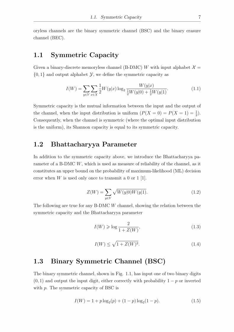
1.3 Binary Symmetric Channel (BSC)
The binary symmetric channel, shown in Fig. 1.1, has input one of two binary digits
(0, 1) and output the input digit, either correctly with probability 1− p or inverted
with p. The symmetric capacity of BSC is
I(W ) = 1 + p log2(p) + (1− p) log2(1− p). (1.5)
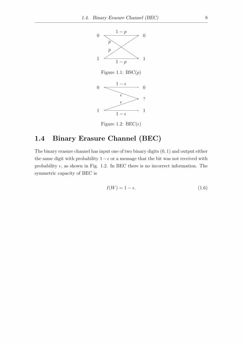
1.4. Binary Erasure Channel (BEC) 8
0
1
0
1
p
p
1− p
1− p
Figure 1.1: BSC(p)
0
1
0
1
?ε
ε
1− ε
1− ε
Figure 1.2: BEC(ε)
1.4 Binary Erasure Channel (BEC)
The binary erasure channel has input one of two binary digits (0, 1) and output either
the same digit with probability 1− ε or a message that the bit was not received with
probability ε, as shown in Fig. 1.2. In BEC there is no incorrect information. The
symmetric capacity of BEC is
I(W ) = 1− ε. (1.6)
9
Chapter 2
Polarization for Binary-input
Channels
Channel polarization is a method for constructing code sequences that achieve the
symmetric capacity I(W ) of any binary-input discrete memoryless channel W . The
symmetric capacity is the highest rate achievable, subject to using the input letters
of the channel with equal probability. In this chapter we will explain the construction
of the Polar codes, proposed by E. Arikan [1].
2.1 Basic Polarization
Channel polarization is an operation by which one manufactures a new set of N
channels {W (i)N : 1 ≤ i ≤ N} out of N independent copies of a given discrete mem-
oryless channel W , that show a polarization effect in the sense that, as N becomes
large, the symmetric capacity terms tend towards 0 or 1 for all but a vanishing
fraction of indices i [1].
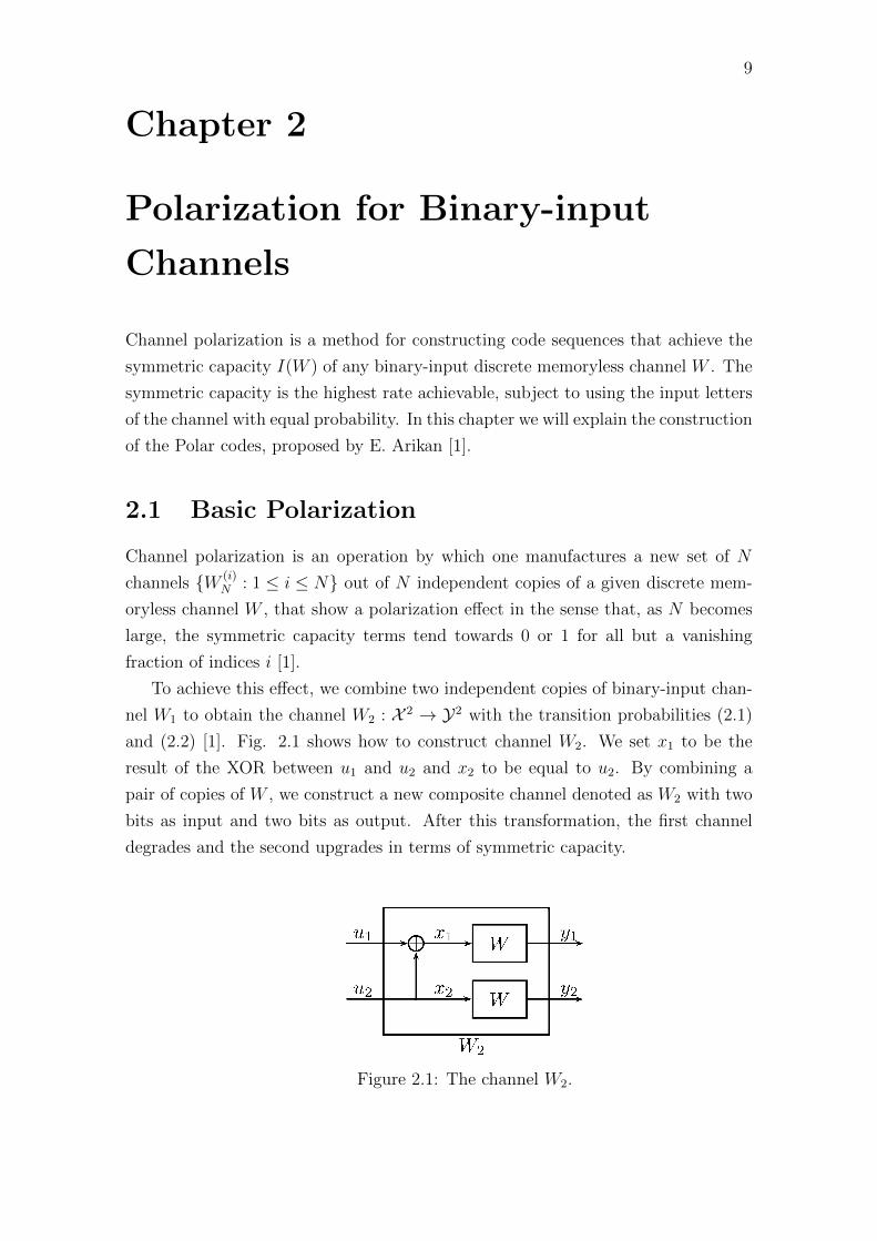
To achieve this effect, we combine two independent copies of binary-input chan-
nel W1 to obtain the channel W2 : X 2 → Y2 with the transition probabilities (2.1)
and (2.2) [1]. Fig. 2.1 shows how to construct channel W2. We set x1 to be the
result of the XOR between u1 and u2 and x2 to be equal to u2. By combining a
pair of copies of W , we construct a new composite channel denoted as W2 with two
bits as input and two bits as output. After this transformation, the first channel
degrades and the second upgrades in terms of symmetric capacity.
Figure 2.1: The channel W2.
2.1. Basic Polarization 10
We define the channel W2 : X 2 → Y2, shown in Fig. 2.1 as
W2(y1, y2|u1, u2) = W2(y1, y2|x1, x2)
= W (y1|x1)W (y2|x2) = W (y1|u1 ⊕ u2)W (y2|u2),
with the following transition probabilities for each channel
W2(1)(y1, y2|u1) =
∑u2
p(y1, y2|u1, u2)p(u2|u1)
=∑u2
p(y1, y2|u1, u2)p(u2)
=1
2p(y1, y2|u1, u2 = 0) +
1
2p(y1, y2|u1, u2 = 1)
=1
2p(y1, y2|x1, x2 = 0) +
1
2p(y1, y2|x1, x2 = 1)
=1
2p(y1|x1)p(y2|x2 = 0) +
1
2p(y1|x1)p(y2|x2 = 1)
=1
2
∑u2
p(y1|x1)p(y2|x2)
=1
2
∑u2
p(y1|u1 ⊕ u2)p(y2|u2), (2.1)
W2(2)(y1, y2, u1|u2) = p(y1, y2|u1, u2)p(u2|u1)
= p(y1, y2|u1, u2)p(u2)
=1
2p(y1, y2|u1, u2)
=1
2p(y1, y2|x1, x2)
=1
2p(y1|x1)p(y2|x2)
=1
2p(y1|u1 ⊕ u2)p(y2|u2), (2.2)
for all u1, u2 ∈ X , y1, y2 ∈ Y , with u1, u2 independent.
In the Appendix, we calculate the previous transition probabilities one-by-one,
for both BSC and BEC, and then we use them in (1.1) to compute the symmetric
capacity of the W2(1) and W2
(2) channels.
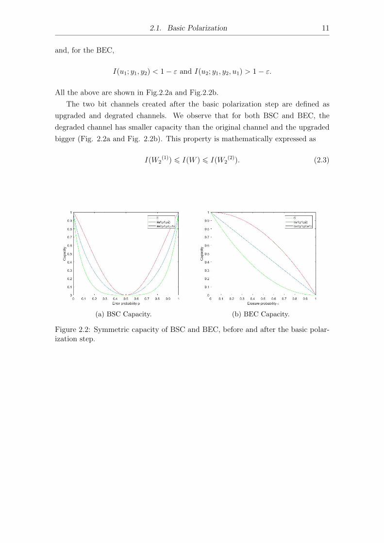
After the calculations, we observe that, for the BSC,
I(u1; y1, y2) < 1−H(p) and I(u2; y1, y2, u1) > 1−H(p)
2.1. Basic Polarization 11
and, for the BEC,
I(u1; y1, y2) < 1− ε and I(u2; y1, y2, u1) > 1− ε.
All the above are shown in Fig.2.2a and Fig.2.2b.
The two bit channels created after the basic polarization step are defined as
upgraded and degrated channels. We observe that for both BSC and BEC, the
degraded channel has smaller capacity than the original channel and the upgraded
bigger (Fig. 2.2a and Fig. 2.2b). This property is mathematically expressed as
I(W2(1)) 6 I(W ) 6 I(W2
(2)). (2.3)
(a) BSC Capacity. (b) BEC Capacity.
Figure 2.2: Symmetric capacity of BSC and BEC, before and after the basic polar-ization step.
2.1. Basic Polarization 12
It is important to mention that the single step channel transformation preserves
the symmetric capacity:
I(W2(1)) + I(W2
(2)) = 2I(W1). (2.4)
Proof.
I(W2(1)) + I(W2
(2)) = I(u1; y1, y2) + I(u2; y1, y2, u1)
= I(u1; y1, y2) + I(u2; y1, y2|u1) + I(u2;u1), according to chain rule
= I(u1; y1, y2) + I(u2; y1, y2|u1), u2, u1 are i.i.d. so I(u2;u1) = 0,
= I(u1, u2; y1, y2)
= I(x1, x2; y1, y2)
= I(x1; y1) + I(x2; y2) = 2I(W1).
Additionally, we can also prove that:
I(W4(1)) + I(W4
(2)) + I(W4(3)) + I(W4
(4)) = 4I(W1) (2.5)
Proof.
I(W4(1)) + I(W4
(2)) + I(W4(3)) + I(W4
(4)) =
= I(u1; y1, y2, y3, y4) + I(u2; y1, y2, y3, y4, u1)+
+ I(u3; y1, y2, y3, y4, u1, u2) + I(u4; y1, y2, y3, y4, u1, u2, u3)
(according to the chain rule),
= I(u1; y1, y2, y3, y4) + I(u2; y1, y2, y3, y4|u1) + I(u2;u1)+
+ I(u3; y1, y2, y3, y4, u2|u1) + I(u3;u1) + I(u4; y1, y2, y3, y4, u2, u3|u1) + I(u4;u1)
(u4, u3, u2, u1 are i.i.d. so I(u2;u1) = I(u3;u1) = I(u4;u1) = 0)
= I(u1; y1, y2, y3, y4) + I(u2; y1, y2, y3, y4) + I(u3; y1, y2, y3, y4|u2)+
+ I(u3;u2) + I(u4; y1, y2, y3, y4, u2|u2) + I(u4;u2)
2.1. Basic Polarization 13
(u4, u3, u2 are i.i.d. so I(u3;u2) = I(u4;u2) = 0)
= I(u1; y1, y2, y3, y4) + I(u2; y1, y2, y3, y4) + I(u3; y1, y2, y3, y4)+
+ I(u4; y1, y2, y3, y4|u3) + I(u4;u3)
(u4, u3 are i.i.d. so I(u2;u3) = 0)
= I(u1; y1, y2, y3, y4) + I(u2; y1, y2, y3, y4) + I(u3; y1, y2, y3, y4) + I(u4; y1, y2, y3, y4)
= I(u1, u2, u3, u4; y1, y2, y3, y4)
= I(x1, x2, x3, x4; y1, y2, y3, y4)
= I(x1; y1) + I(x2; y2) + I(x3; y3) + I(x4; y4) = 4I(W1).
Finally, the above properties can be generalized for N bits:
N∑i=1
I(WN(i)) = NI(W ) (2.6)
Proof.
N∑i=1
I(WN(i)) = I(u1; y
N1 ) + I(u2; y
N1 , u1) + I(u3; y
N1 , u1, u2) + ...+ I(uN ; yN1 , u
N−11 )
= I(u1; yN1 ) + I(u2; y
N1 |u1) + ...+ I(uN ; yN1 |uN−11 )
= I(u1...uN ; y1...yN) = I(x1...xN ; y1, ...yN)
= I(x1; y1) + I(x2; y2) + I(x3; y3) + ...+ I(xN ; yN) = NI(W )
with u1, u2, ..., un i.i.d.
2.1. Basic Polarization 14
For the BEC, the following two properties are true
I(W2(1)) = I(W )2, (2.7)
I(W2(2)) = 2I(W )− I(W )2. (2.8)
Proof.
According to (1.2),
Z(W2(2)) =
∑y21 ,u1
1
2
√W2
(2)(y1, y2, u1|0)√W2
(2)(y1, y2, u1|1)
=∑y21 ,u1
1
2
√W (y1|u1 ⊕ 0)W (y2|0)
√W (y1|u1 ⊕ 1)W (y2|1)
=∑y21 ,u1
1
2
√W (y1|u1)W (y2|0)
√W (y1|u1 ⊕ 1)W (y2|1)
=∑y2
√W (y2|0)W (y2|1)
∑u1
1
2
∑y1
√W (y1|u1)W (y1|u1 ⊕ 1)
= Z(W ) · 1 · Z(W )
= Z(W )2
For any BEC(ε) W, Z(W ) = ε,
Z(W ) =∑yεΥ
√W (y|0)W (y|1)
=√W (0|0)W (0|1) +
√W (e|0)W (e|1) +
√W (1|0)W (1|1)
=√
(1− ε) · 0 +√ε · ε+
√0 · (1− ε)
= ε
We also know that the symmetric capacity of BEC is
I(W ) = 1− ε.
2.1. Basic Polarization 15
We conclude that Z(W ) = 1− I(W ) for BEC.
Z(W2(2)) = Z(W )2 ⇔
⇔ 1− I(W2(2)) = (1− I(W ))2
⇔ 1− I(W2(2)) = 1 + I(W )2 − 2I(W )
⇔ I(W2(2)) = 2I(W )− I(W )2
considering that 2I(W ) = I(W2(1)) + I(W2
(2)), we can also prove that
I(W2(1)) = I(W )2.
2.1. Basic Polarization 16
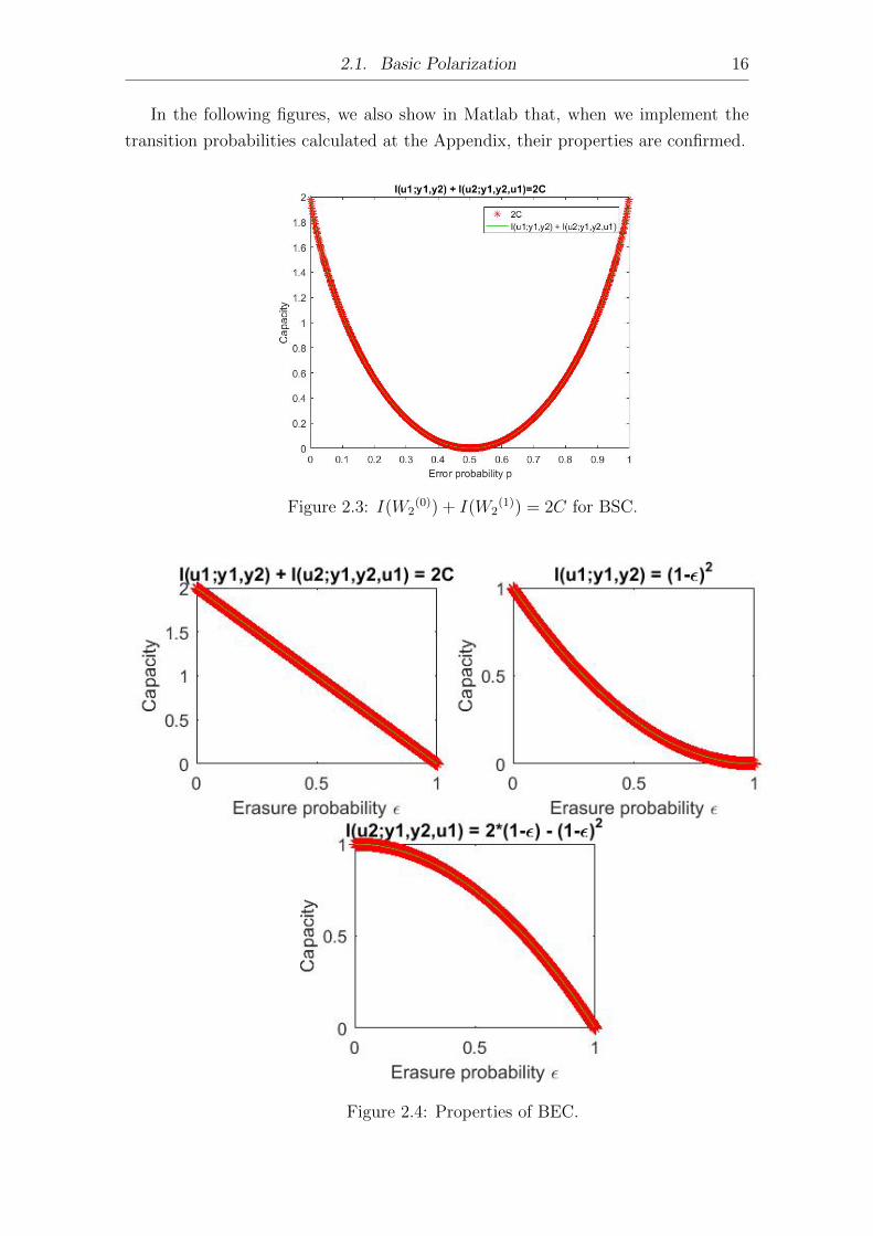
In the following figures, we also show in Matlab that, when we implement the
transition probabilities calculated at the Appendix, their properties are confirmed.
Figure 2.3: I(W2(0)) + I(W2
(1)) = 2C for BSC.
Figure 2.4: Properties of BEC.
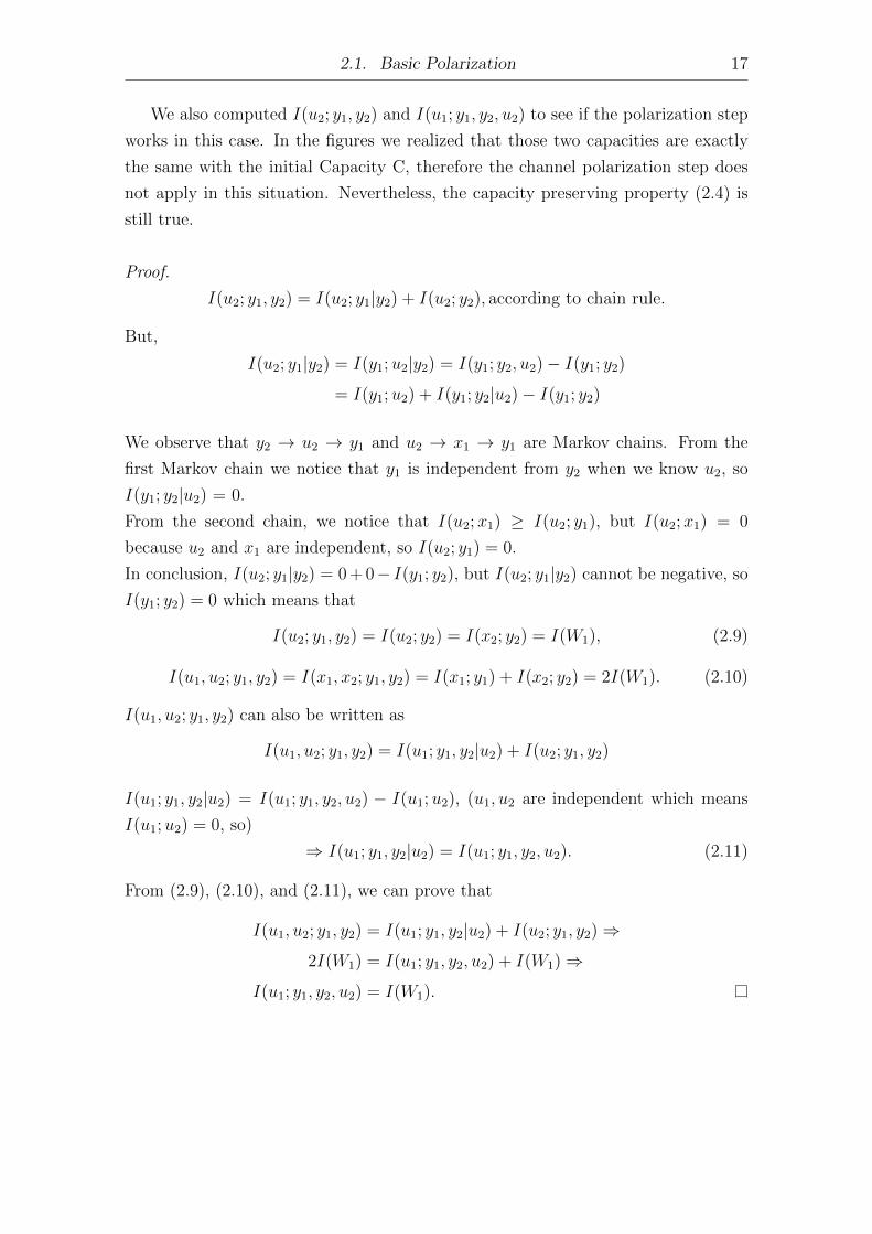
2.1. Basic Polarization 17
We also computed I(u2; y1, y2) and I(u1; y1, y2, u2) to see if the polarization step
works in this case. In the figures we realized that those two capacities are exactly
the same with the initial Capacity C, therefore the channel polarization step does
not apply in this situation. Nevertheless, the capacity preserving property (2.4) is
still true.
Proof.
I(u2; y1, y2) = I(u2; y1|y2) + I(u2; y2), according to chain rule.
But,
I(u2; y1|y2) = I(y1;u2|y2) = I(y1; y2, u2)− I(y1; y2)
= I(y1;u2) + I(y1; y2|u2)− I(y1; y2)
We observe that y2 → u2 → y1 and u2 → x1 → y1 are Markov chains. From the
first Markov chain we notice that y1 is independent from y2 when we know u2, so
I(y1; y2|u2) = 0.
From the second chain, we notice that I(u2;x1) ≥ I(u2; y1), but I(u2;x1) = 0
because u2 and x1 are independent, so I(u2; y1) = 0.
In conclusion, I(u2; y1|y2) = 0 + 0− I(y1; y2), but I(u2; y1|y2) cannot be negative, so
I(y1; y2) = 0 which means that
I(u2; y1, y2) = I(u2; y2) = I(x2; y2) = I(W1), (2.9)
I(u1, u2; y1, y2) = I(x1, x2; y1, y2) = I(x1; y1) + I(x2; y2) = 2I(W1). (2.10)
I(u1, u2; y1, y2) can also be written as
I(u1, u2; y1, y2) = I(u1; y1, y2|u2) + I(u2; y1, y2)
I(u1; y1, y2|u2) = I(u1; y1, y2, u2) − I(u1;u2), (u1, u2 are independent which means
I(u1;u2) = 0, so)
⇒ I(u1; y1, y2|u2) = I(u1; y1, y2, u2). (2.11)
From (2.9), (2.10), and (2.11), we can prove that
I(u1, u2; y1, y2) = I(u1; y1, y2|u2) + I(u2; y1, y2)⇒
2I(W1) = I(u1; y1, y2, u2) + I(W1)⇒
I(u1; y1, y2, u2) = I(W1).
2.1. Basic Polarization 18
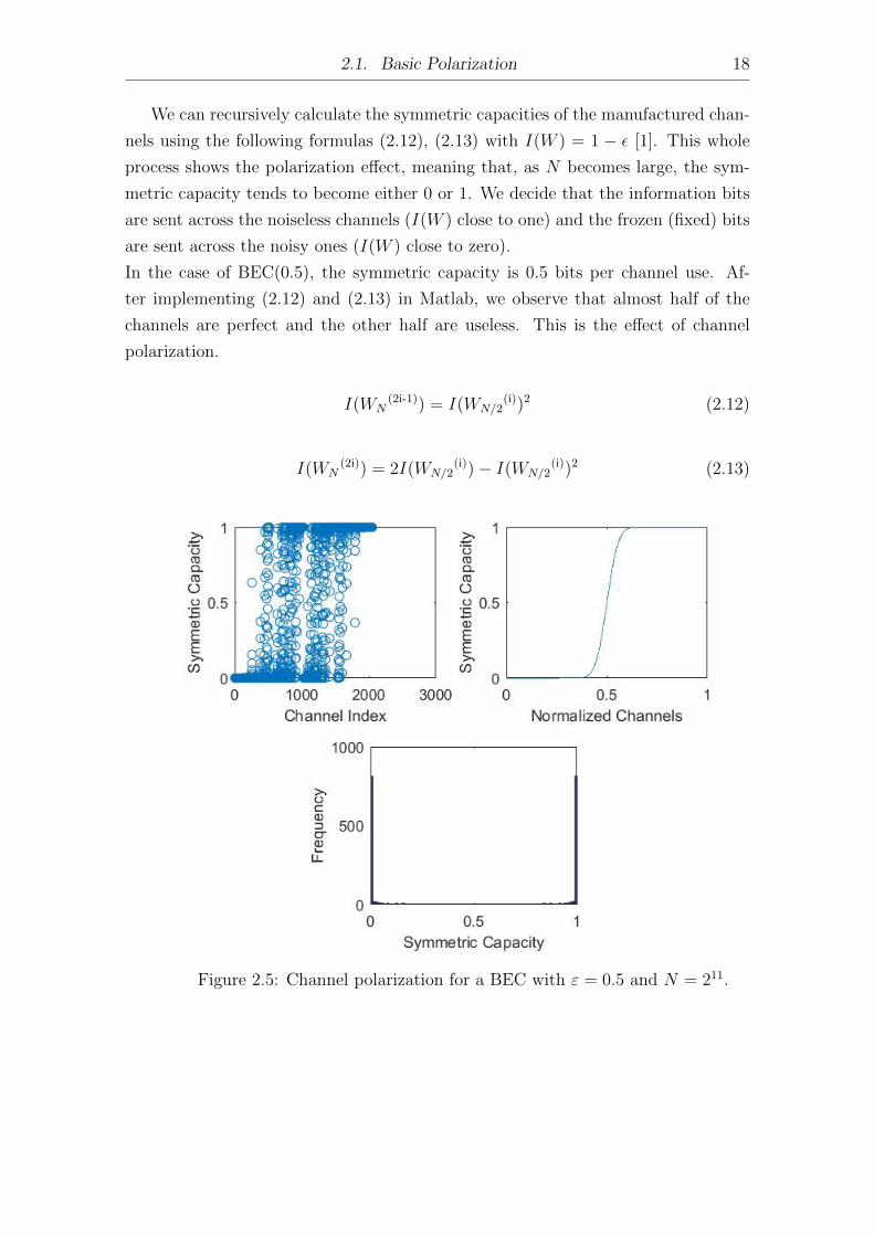
We can recursively calculate the symmetric capacities of the manufactured chan-
nels using the following formulas (2.12), (2.13) with I(W ) = 1 − ε [1]. This whole
process shows the polarization effect, meaning that, as N becomes large, the sym-
metric capacity tends to become either 0 or 1. We decide that the information bits
are sent across the noiseless channels (I(W ) close to one) and the frozen (fixed) bits
are sent across the noisy ones (I(W ) close to zero).
In the case of BEC(0.5), the symmetric capacity is 0.5 bits per channel use. Af-
ter implementing (2.12) and (2.13) in Matlab, we observe that almost half of the
channels are perfect and the other half are useless. This is the effect of channel
polarization.
I(WN(2i-1)) = I(WN/2
(i))2 (2.12)
I(WN(2i)) = 2I(WN/2
(i))− I(WN/2(i))2 (2.13)
Figure 2.5: Channel polarization for a BEC with ε = 0.5 and N = 211.
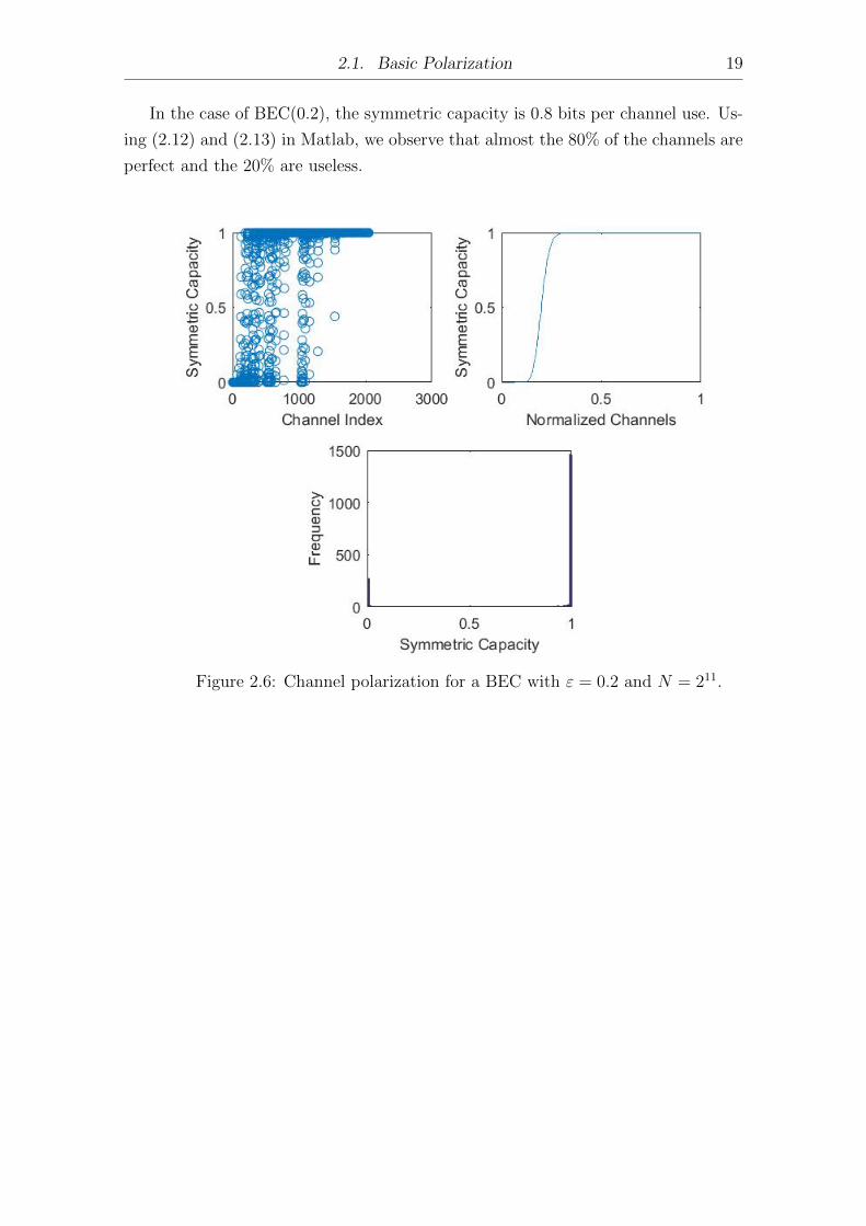
2.1. Basic Polarization 19
In the case of BEC(0.2), the symmetric capacity is 0.8 bits per channel use. Us-
ing (2.12) and (2.13) in Matlab, we observe that almost the 80% of the channels are
perfect and the 20% are useless.
Figure 2.6: Channel polarization for a BEC with ε = 0.2 and N = 211.
2.2. Encoding 20
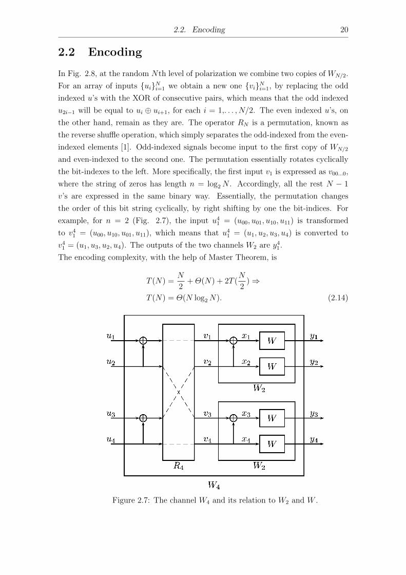
2.2 Encoding
In Fig. 2.8, at the random Nth level of polarization we combine two copies of WN/2.
For an array of inputs {ui}Ni=1 we obtain a new one {vi}Ni=1, by replacing the odd
indexed u’s with the XOR of consecutive pairs, which means that the odd indexed
u2i−1 will be equal to ui ⊕ ui+1, for each i = 1,. . . , N/2. The even indexed u’s, on
the other hand, remain as they are. The operator RN is a permutation, known as
the reverse shuffle operation, which simply separates the odd-indexed from the even-
indexed elements [1]. Odd-indexed signals become input to the first copy of WN/2
and even-indexed to the second one. The permutation essentially rotates cyclically
the bit-indexes to the left. More specifically, the first input v1 is expressed as v00...0,
where the string of zeros has length n = log2N . Accordingly, all the rest N − 1
v’s are expressed in the same binary way. Essentially, the permutation changes
the order of this bit string cyclically, by right shifting by one the bit-indices. For
example, for n = 2 (Fig. 2.7), the input u41 = (u00, u01, u10, u11) is transformed
to v41 = (u00, u10, u01, u11), which means that u41 = (u1, u2, u3, u4) is converted to
v41 = (u1, u3, u2, u4). The outputs of the two channels W2 are y41.
The encoding complexity, with the help of Master Theorem, is
T (N) =N
2+Θ(N) + 2T (
N
2)⇒
T (N) = Θ(N log2N). (2.14)
Figure 2.7: The channel W4 and its relation to W2 and W .
2.2. Encoding 21
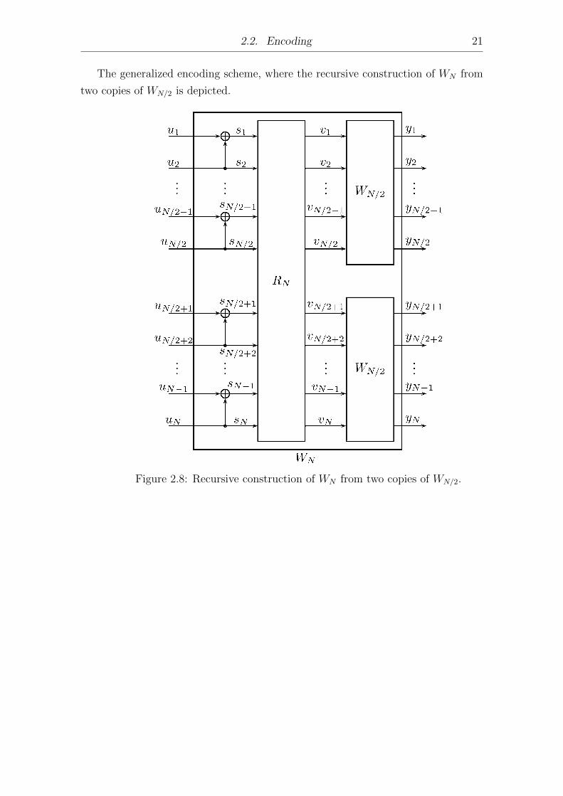
The generalized encoding scheme, where the recursive construction of WN from
two copies of WN/2 is depicted.
Figure 2.8: Recursive construction of WN from two copies of WN/2.
2.3. Successive Cancellation Decoding 22
2.3 Successive Cancellation Decoding
The successive cancellation (SC) decoder, introduced in [1], decides with the rule
of closest neighbor on the ith bit (1 ≤ i ≤ N) that is transmitted over W(i)N , by
computing (2.15) and (2.16) for BEC and (2.17) and (2.18) for BSC.
More specifically, for the BEC with erasure probability ε, first we use the recur-
sive formulas of the symmetric capacity (2.12), (2.13). After the recursive calcu-
lation, we assign the frozen bits (usually 0’s) wherever the capacity has its lowest
prices, so that we can use the good channels (those with high capacity) to transmit
the information bits.
To decode successfully, we calculate the transition probabilities by using the
efficient recursive formulas (2.15), (2.16). Each estimation is carried out by using
the knowledge of frozen and previously estimated symbols. More specifically, if ui
is a frozen bit, then ui takes the value of ui, and, if ui is an information bit, then
the decoder computes the transition probabilities for BEC or the likelihood ratios
(LR) for BSC.
We implemented two decoding approaches, a slow (complexity O(N2)) and a
fast (complexity O(N log2N)). In the slow decoder, we store each calculation of
(2.15) and (2.16) in a matrix and we estimate the original value of u by comparing
W(i)N (yN1 , u
i−11 |0) and W
(i)N (yN1 , u
i−11 |1). The fast, on the contrary, was generated by
observing that several computed values are calculated more than one time, so we
store them in a cell array of size N × (log2N + 1) to avoid recalculation and to use
the stored values when needed. In each cell, both probabilities W(i)N (yN1 , u
i−11 |0) and
W(i)N (yN1 , u
i−11 |1), are stored so that we can compare them easily and use them for the
calculations. Each cell is filled after Θ(1) calculations, which implies that the com-
plexity of this decoding is O(N log2N). The calculation of a probability at length
N for both decoders is reduced to the calculation of two probabilities. Accordingly,
at length N/2, each calculation of a probability at length N/2 requires the calcula-
tion of two probabilities at length N/4 and so on. This recursion can be computed
until it reaches the block length 1, at which point we calculate W (yi|0) and W (yi|1).
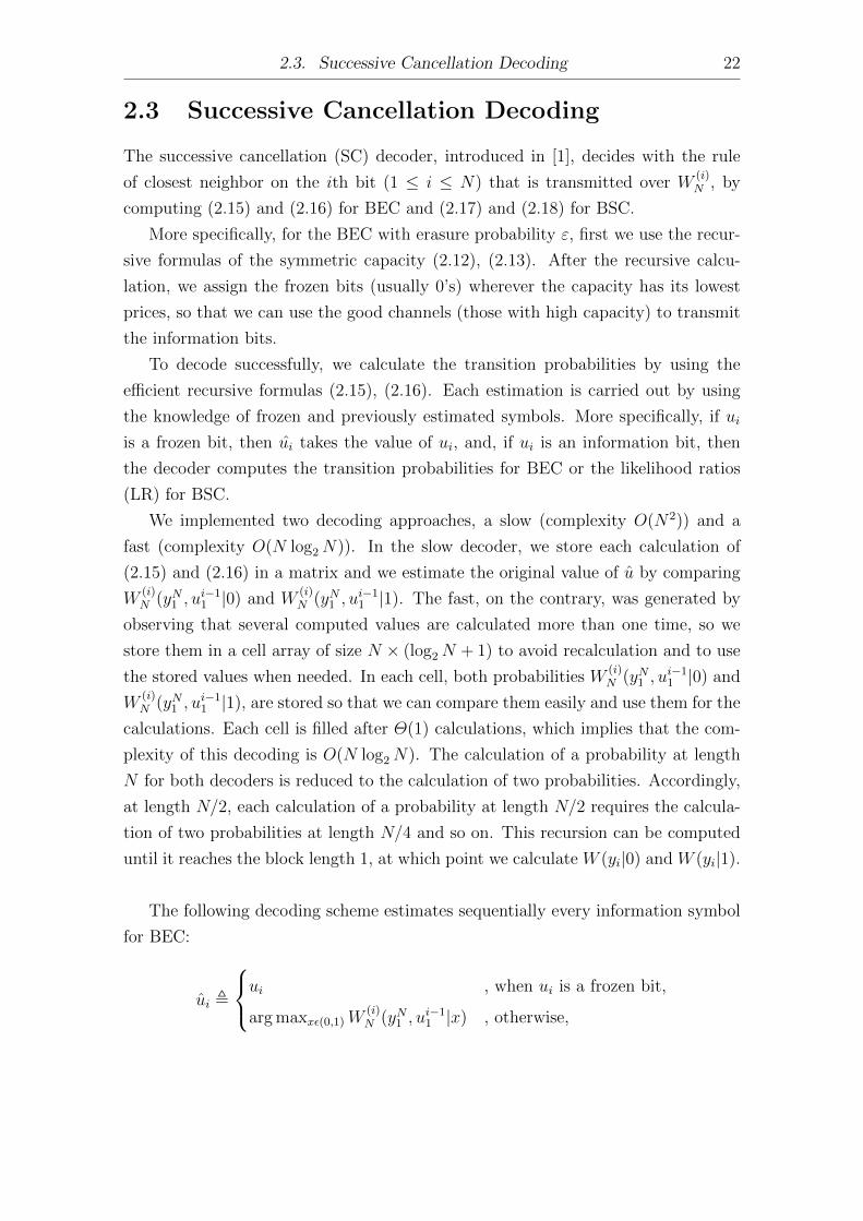
The following decoding scheme estimates sequentially every information symbol
for BEC:
ui ,
ui , when ui is a frozen bit,
arg maxxε(0,1)W(i)N (yN1 , u
i−11 |x) , otherwise,
2.3. Successive Cancellation Decoding 23
using the recursive formulas
W(2i−1)2N (y2N1 , u2i−21 |u2i−1) =
∑u2i
1
2W
(i)N (yN1 , u
2i−21,o ⊕ u2i−21,e |u2i−1 ⊕ u2i)
·W (i)N (y2NN+1, u
2i−21,e |u2i), (2.15)
and
W(2i)2N (y2N1 , u2i−11 |u2i) =
1
2W
(i)N (yN1 , u
2i−21,o ⊕ u2i−21,e |u2i−1 ⊕ u2i) ·W
(i)N (y2NN+1, u
2i−21,e |u2i).
(2.16)
For the BSC, we followed the same procedure as in BEC for the slow decoder.
For the fast decoder, we also took advantage of the fact that some of the recursions
were calculated more than once, with the only difference being the storage of the
computations in an array. The decoded ui for BSC is estimated as
ui
ui , if ui is a frozen bit,
0 , if L(i)N (yN1 , u
i−11 ) ≥ 1,
1 , otherwise.
The likelihood ratio is defined as
L(i)N (yN1 , u
i−11 ) =
W(i)N (yN1 , u
i−11 |0)
W(i)N (yN1 , u
i−11 |1)
.
To estimate L(i)N (yN1 , u
i−11 ), we use the recursive formulas
L(2i−1)N (yN1 , u
2i−21 ) =
L(i)N/2(y
N/21 , u2i−21,o ⊕ u2i−21,e )L
(i)N/2(y
NN/2+1, u
2i−21,e ) + 1
L(i)N/2(y
N/21 , u2i−21,o ⊕ u2i−21,e ) + L
(i)N/2(y
NN/2+1, u
2i−21,e )
(2.17)
and
L(2i)N (yN1 , u
2i−11 ) = [L
(i)N/2(y
N/21 , u2i−21,o ⊕ u2i−21,e )]1−2u2i−1 · L(i)
N/2(yNN/2+1, u
2i−21,e ). (2.18)
At the Nth level, each calculation of a LR at length N is reduced to the calcula-
tion of two LRs at length N/2, each calculation of a LR at length N/2 is reduced to
the calculation of two LRs at length N/4 and so on. This recursion can be computed
down to block length 1, at which point the LRs have the form
L(1)1 (y1) =
W (yi|0)
W (yi|1).
2.4. Performance on BEC 24
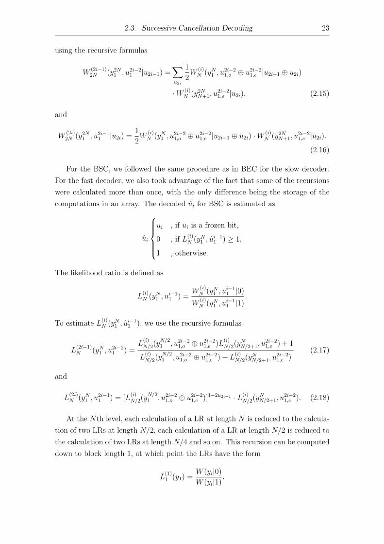
2.4 Performance on BEC
In Fig. 2.4, we observe the improvement of the BER performance as the block
length grows larger. This happens because perfect channel polarization is accom-
plished when the block length increases to infinity.
Figure 2.9: BER of transmissions over BEC, with rate = 0.5.
2.5. Application of Polar Coding to the Degraded Broadcast Binary Erasure Channel25
-Tx
-
C1-
C2-
R1
R2
Figure 2.10: Signal model
2.5 Application of Polar Coding to the Degraded
Broadcast Binary Erasure Channel
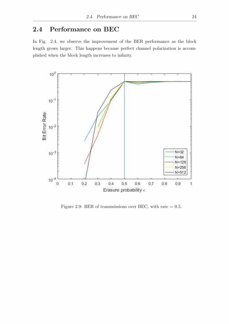
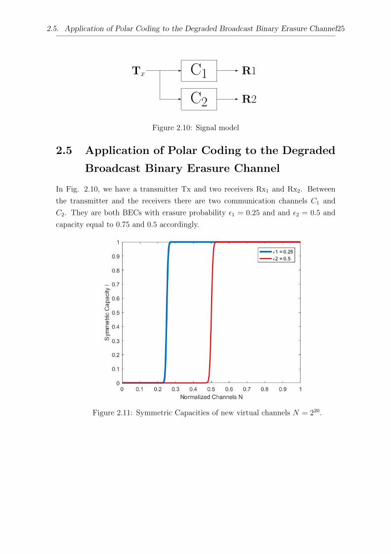
In Fig. 2.10, we have a transmitter Tx and two receivers Rx1 and Rx2. Between
the transmitter and the receivers there are two communication channels C1 and
C2. They are both BECs with erasure probability ε1 = 0.25 and and ε2 = 0.5 and
capacity equal to 0.75 and 0.5 accordingly.
Figure 2.11: Symmetric Capacities of new virtual channels N = 220.
2.5. Application of Polar Coding to the Degraded Broadcast Binary Erasure Channel26
-X1
-X2
-XN
W
W
W
-Y1
-Y2
-YN
publicbits
bit-channels good forboth R1 and R2
privatebits
bit-channels good forR1 but bad for R2
frozenbits
bit-channels bad forboth R1 and R2
...
...
...
...
...
...
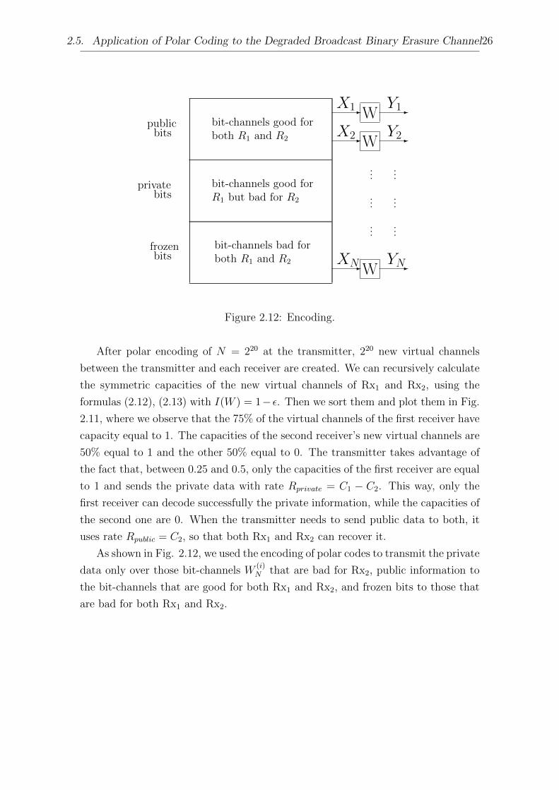
Figure 2.12: Encoding.
After polar encoding of N = 220 at the transmitter, 220 new virtual channels
between the transmitter and each receiver are created. We can recursively calculate
the symmetric capacities of the new virtual channels of Rx1 and Rx2, using the
formulas (2.12), (2.13) with I(W ) = 1− ε. Then we sort them and plot them in Fig.
2.11, where we observe that the 75% of the virtual channels of the first receiver have
capacity equal to 1. The capacities of the second receiver’s new virtual channels are
50% equal to 1 and the other 50% equal to 0. The transmitter takes advantage of
the fact that, between 0.25 and 0.5, only the capacities of the first receiver are equal
to 1 and sends the private data with rate Rprivate = C1 − C2. This way, only the
first receiver can decode successfully the private information, while the capacities of
the second one are 0. When the transmitter needs to send public data to both, it
uses rate Rpublic = C2, so that both Rx1 and Rx2 can recover it.
As shown in Fig. 2.12, we used the encoding of polar codes to transmit the private
data only over those bit-channels W(i)N that are bad for Rx2, public information to
the bit-channels that are good for both Rx1 and Rx2, and frozen bits to those that
are bad for both Rx1 and Rx2.
27
Appendix
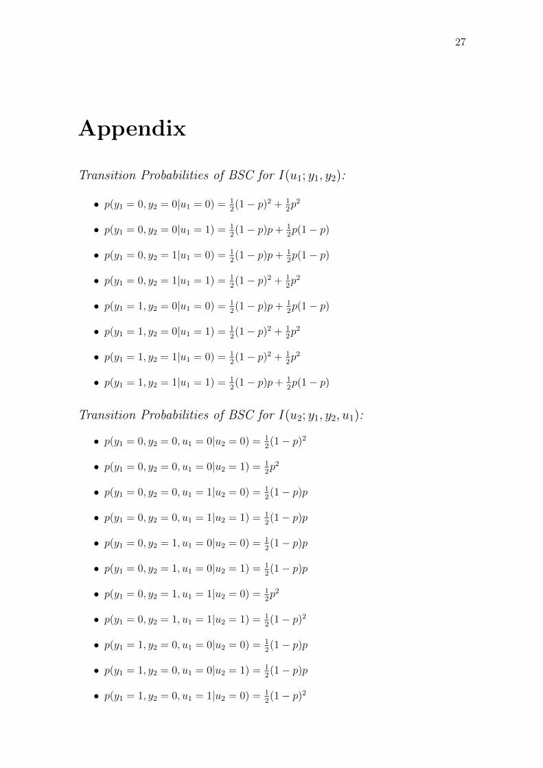
Transition Probabilities of BSC for I(u1; y1, y2):
• p(y1 = 0, y2 = 0|u1 = 0) = 12(1− p)2 + 1
2p2
• p(y1 = 0, y2 = 0|u1 = 1) = 12(1− p)p+ 1
2p(1− p)
• p(y1 = 0, y2 = 1|u1 = 0) = 12(1− p)p+ 1
2p(1− p)
• p(y1 = 0, y2 = 1|u1 = 1) = 12(1− p)2 + 1
2p2
• p(y1 = 1, y2 = 0|u1 = 0) = 12(1− p)p+ 1
2p(1− p)
• p(y1 = 1, y2 = 0|u1 = 1) = 12(1− p)2 + 1
2p2
• p(y1 = 1, y2 = 1|u1 = 0) = 12(1− p)2 + 1
2p2
• p(y1 = 1, y2 = 1|u1 = 1) = 12(1− p)p+ 1
2p(1− p)
Transition Probabilities of BSC for I(u2; y1, y2, u1):
• p(y1 = 0, y2 = 0, u1 = 0|u2 = 0) = 12(1− p)2
• p(y1 = 0, y2 = 0, u1 = 0|u2 = 1) = 12p2
• p(y1 = 0, y2 = 0, u1 = 1|u2 = 0) = 12(1− p)p
• p(y1 = 0, y2 = 0, u1 = 1|u2 = 1) = 12(1− p)p
• p(y1 = 0, y2 = 1, u1 = 0|u2 = 0) = 12(1− p)p
• p(y1 = 0, y2 = 1, u1 = 0|u2 = 1) = 12(1− p)p
• p(y1 = 0, y2 = 1, u1 = 1|u2 = 0) = 12p2
• p(y1 = 0, y2 = 1, u1 = 1|u2 = 1) = 12(1− p)2
• p(y1 = 1, y2 = 0, u1 = 0|u2 = 0) = 12(1− p)p
• p(y1 = 1, y2 = 0, u1 = 0|u2 = 1) = 12(1− p)p
• p(y1 = 1, y2 = 0, u1 = 1|u2 = 0) = 12(1− p)2
Appendix 28
• p(y1 = 1, y2 = 0, u1 = 1|u2 = 1) = 12p2
• p(y1 = 1, y2 = 1, u1 = 0|u2 = 0) = 12p2
• p(y1 = 1, y2 = 1, u1 = 0|u2 = 1) = 12(1− p)2
• p(y1 = 1, y2 = 1, u1 = 1|u2 = 0) = 12(1− p)p
• p(y1 = 1, y2 = 1, u1 = 1|u2 = 1) = 12(1− p)p
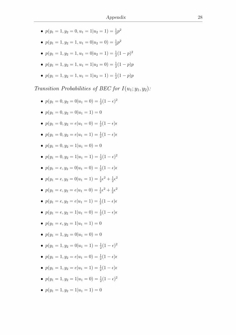
Transition Probabilities of BEC for I(u1; y1, y2):
• p(y1 = 0, y2 = 0|u1 = 0) = 12(1− ε)2
• p(y1 = 0, y2 = 0|u1 = 1) = 0
• p(y1 = 0, y2 = e|u1 = 0) = 12(1− ε)ε
• p(y1 = 0, y2 = e|u1 = 1) = 12(1− ε)ε
• p(y1 = 0, y2 = 1|u1 = 0) = 0
• p(y1 = 0, y2 = 1|u1 = 1) = 12(1− ε)2
• p(y1 = e, y2 = 0|u1 = 0) = 12(1− ε)ε
• p(y1 = e, y2 = 0|u1 = 1) = 12ε2 + 1
2ε2
• p(y1 = e, y2 = e|u1 = 0) = 12ε2 + 1
2ε2
• p(y1 = e, y2 = e|u1 = 1) = 12(1− ε)ε
• p(y1 = e, y2 = 1|u1 = 0) = 12(1− ε)ε
• p(y1 = e, y2 = 1|u1 = 1) = 0
• p(y1 = 1, y2 = 0|u1 = 0) = 0
• p(y1 = 1, y2 = 0|u1 = 1) = 12(1− ε)2
• p(y1 = 1, y2 = e|u1 = 0) = 12(1− ε)ε
• p(y1 = 1, y2 = e|u1 = 1) = 12(1− ε)ε
• p(y1 = 1, y2 = 1|u1 = 0) = 12(1− ε)2
• p(y1 = 1, y2 = 1|u1 = 1) = 0
Appendix 29
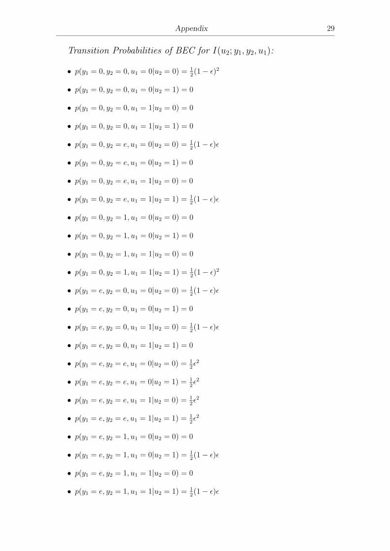
Transition Probabilities of BEC for I(u2; y1, y2, u1):
• p(y1 = 0, y2 = 0, u1 = 0|u2 = 0) = 12(1− ε)2
• p(y1 = 0, y2 = 0, u1 = 0|u2 = 1) = 0
• p(y1 = 0, y2 = 0, u1 = 1|u2 = 0) = 0
• p(y1 = 0, y2 = 0, u1 = 1|u2 = 1) = 0
• p(y1 = 0, y2 = e, u1 = 0|u2 = 0) = 12(1− ε)ε
• p(y1 = 0, y2 = e, u1 = 0|u2 = 1) = 0
• p(y1 = 0, y2 = e, u1 = 1|u2 = 0) = 0
• p(y1 = 0, y2 = e, u1 = 1|u2 = 1) = 12(1− ε)ε
• p(y1 = 0, y2 = 1, u1 = 0|u2 = 0) = 0
• p(y1 = 0, y2 = 1, u1 = 0|u2 = 1) = 0
• p(y1 = 0, y2 = 1, u1 = 1|u2 = 0) = 0
• p(y1 = 0, y2 = 1, u1 = 1|u2 = 1) = 12(1− ε)2
• p(y1 = e, y2 = 0, u1 = 0|u2 = 0) = 12(1− ε)ε
• p(y1 = e, y2 = 0, u1 = 0|u2 = 1) = 0
• p(y1 = e, y2 = 0, u1 = 1|u2 = 0) = 12(1− ε)ε
• p(y1 = e, y2 = 0, u1 = 1|u2 = 1) = 0
• p(y1 = e, y2 = e, u1 = 0|u2 = 0) = 12ε2
• p(y1 = e, y2 = e, u1 = 0|u2 = 1) = 12ε2
• p(y1 = e, y2 = e, u1 = 1|u2 = 0) = 12ε2
• p(y1 = e, y2 = e, u1 = 1|u2 = 1) = 12ε2
• p(y1 = e, y2 = 1, u1 = 0|u2 = 0) = 0
• p(y1 = e, y2 = 1, u1 = 0|u2 = 1) = 12(1− ε)ε
• p(y1 = e, y2 = 1, u1 = 1|u2 = 0) = 0
• p(y1 = e, y2 = 1, u1 = 1|u2 = 1) = 12(1− ε)ε
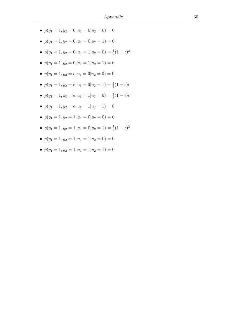
Appendix 30
• p(y1 = 1, y2 = 0, u1 = 0|u2 = 0) = 0
• p(y1 = 1, y2 = 0, u1 = 0|u2 = 1) = 0
• p(y1 = 1, y2 = 0, u1 = 1|u2 = 0) = 12(1− ε)2
• p(y1 = 1, y2 = 0, u1 = 1|u2 = 1) = 0
• p(y1 = 1, y2 = e, u1 = 0|u2 = 0) = 0
• p(y1 = 1, y2 = e, u1 = 0|u2 = 1) = 12(1− ε)ε
• p(y1 = 1, y2 = e, u1 = 1|u2 = 0) = 12(1− ε)ε
• p(y1 = 1, y2 = e, u1 = 1|u2 = 1) = 0
• p(y1 = 1, y2 = 1, u1 = 0|u2 = 0) = 0
• p(y1 = 1, y2 = 1, u1 = 0|u2 = 1) = 12(1− ε)2
• p(y1 = 1, y2 = 1, u1 = 1|u2 = 0) = 0
• p(y1 = 1, y2 = 1, u1 = 1|u2 = 1) = 0
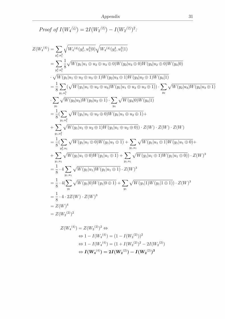
Appendix 31
Proof of I(W4(4)) = 2I(W2
(2))− I(W2(2))2:
Z(W4(4)) =
∑y41 ,u
31
√W4
(4)(y41, u31|0)
√W4
(4)(y41, u31|1)
=∑y41 ,u
31
1
8
√W (y1|u1 ⊕ u2 ⊕ u3 ⊕ 0)W (y2|u3 ⊕ 0)W (y3|u2 ⊕ 0)W (y4|0)
·√W (y1|u1 ⊕ u2 ⊕ u3 ⊕ 1)W (y2|u3 ⊕ 1)W (y3|u2 ⊕ 1)W (y4|1)
=1
8
∑y1,u31
(√W (y1|u1 ⊕ u2 ⊕ u3)W (y1|u1 ⊕ u2 ⊕ u3 ⊕ 1)) ·
∑y2
√W (y2|u3)W (y2|u3 ⊕ 1)
·∑y3
√W (y3|u2)W (y3|u2 ⊕ 1) ·
∑y4
√W (y4|0)W (y4|1)
=1
8(∑y1,u21
√W (y1|u1 ⊕ u2 ⊕ 0)W (y1|u1 ⊕ u2 ⊕ 1)+
+∑y1,u21
√W (y1|u1 ⊕ u2 ⊕ 1)W (y1|u1 ⊕ u2 ⊕ 0)) · Z(W ) · Z(W ) · Z(W )
=1
8(∑y21 ,u1
√W (y1|u1 ⊕ 0)W (y1|u1 ⊕ 1) +
∑y1,u1
√W (y1|u1 ⊕ 1)W (y1|u1 ⊕ 0)+
+∑y1,u1
√W (y1|u1 ⊕ 0)W (y1|u1 ⊕ 1) +
∑y1,u1
√W (y1|u1 ⊕ 1)W (y1|u1 ⊕ 0)) · Z(W )3
=1
8· 4
∑y1,u1
√W (y1|u1)W (y1|u1 ⊕ 1) · Z(W )3
=1
8· 4(
∑y1
√W (y1|0)W (y1|0⊕ 1) +
∑y1
√W (y1|1)W (y1|1⊕ 1)) · Z(W )3
=1
8· 4 · 2Z(W ) · Z(W )3
= Z(W )4
= Z(W2(2))2
Z(W4(4)) = Z(W2
(2))2 ⇔
⇔ 1− I(W4(4)) = (1− I(W2
(2)))2
⇔ 1− I(W4(4)) = (1 + I(W2
(2))2 − 2I(W2(2))
⇔ I(W4(4)) = 2I(W2
(2))− I(W2(2))2
32
Bibliography
[1] E. Arikan. Channel polarization: A method for constructing capacity-achieving
codes for symmetric binary-input memoryless channels. IEEE Transactions on
Information Theory, 55(7):3051–3073, 2009.
[2] A. Carlton. Surprise! polar codes are coming in from the cold, 2016 (ac-
cessed May 2018). https://www.computerworld.com/article/3151866/
mobile-wireless/surprise-polar-codes-are-coming-in-from-the-cold.
html
[3] A. Carlton. How polar codes work, 2017 (accessed May 2018).
https://www.computerworld.com/article/3228804/mobile-wireless/
how-polar-codes-work.html#tk.drr_mlt
[4] R. A. Chou and M. R. Bloch. Polar coding for the broadcast channel with confi-
dential messages: A random binning analogy. IEEE Transactions on Information
Theory, 62(5):2410–2429, 2016.
[5] Y. Fountzoulas, A. Kosta, and G. N. Karystinos. Polar-code-based security
on the bsc-modeled harq in fading. In Telecommunications (ICT), 2016 23rd
International Conference on, 1–5, IEEE, 2016.
[6] C. Leroux, A. J. Raymond, G. Sarkis, I. Tal, A. Vardy, and W. J. Gross. Hard-
ware implementation of successive-cancellation decoders for polar codes. Journal
of Signal Processing Systems, 69(3):305–315, 2012.
[7] H. Mahdavifar and A. Vardy. Achieving the secrecy capacity of wiretap channels
using polar codes. IEEE Transactions on Information Theory, 57(10):6428–6443,
2011.
[8] C. E. Shannon. Communication theory of secrecy systems. Bell Labs Technical
Journal, 28(4):656–715, 1949.
[9] A. D. Wyner. The wire-tap channel. Bell Labs Technical Journal, 54(8):1355–
1387, 1975.