Poisson’s ratio in cubic materials

BY ANDREW N. NORRIS*

Mechanical and Aerospace Engineering, Rutgers University, Piscataway,NJ 08854-8058, USA

Expressions are given for the maximum and minimum values of Poisson’s ratio n formaterials with cubic symmetry. Values less than K1 occur if and only if the maximumshear modulus is associated with the cube axis and is at least 25 times the value of theminimum shear modulus. Large values of jnj occur in directions at which the Youngmodulus is approximately equal to one half of its 111 value. Such directions, by theirnature, are very close to 111. Application to data for cubic crystals indicates that certainIndium Thallium alloys simultaneously exhibit Poisson’s ratio less than K1 and greaterthan C2.

Keywords: Poisson’s ratio; cubic symmetry; anisotropy

*no

RecAcc

1. Introduction

The Poisson’s ratio n is an important physical quantity in the mechanics ofsolids, arguably second only in significance to the Young modulus. It is strictlybounded between K1 and 1/2 in isotropic solids, but no such simple bounds existfor anisotropic solids, even for those closest to isotropy in material symmetry:cubic materials. In fact, Ting & Chen (2005) demonstrated that arbitrarily largepositive and negative values of Poisson’s ratio could occur in solids with cubicmaterial symmetry. The key requirement is that the Young modulus in the 111-direction is very large (relative to other directions), and as a consequence thePoisson’s ratio for stretch close to but not coincident with the 111-direction canbe large, positive or negative. Ting & Chen’s result replaces conventional wisdom(e.g. Baughman et al. 1998) that the extreme values of n are associated withstretch along the face diagonal (110-direction). Boulanger & Hayes (1998)showed that arbitrarily large values of jnj are possible in materials oforthorhombic symmetry. Both pairs of authors analytically constructed sets ofelastic moduli, which show the unusual properties while still physicallyadmissible. The dependence of the large values of Poisson’s ratio on elasticmoduli and the related scalings of strain are discussed by Ting (2004) for cubicand more anisotropic materials.

To date there is no anisotropic elastic symmetry for which there are analyticexpressions of the extreme values of Poisson’s ratio for all materials in thesymmetry class, although bounds may be obtained for some specific pairs ofdirections for certain material symmetries. For instance, Lempriere (1968)

Proc. R. Soc. A (2006) 462, 3385–3405

doi:10.1098/rspa.2006.1726

Published online 30 May 2006

rris@rutgers.edu

eived 22 July 2005epted 28 March 2006 3385 q 2006 The Royal Society

A. N. Norris3386

considered Poisson’s ratios for stretch and transverse strain along the principaldirections, and showed that it is bounded by the square root of the ratio of

principal Young’s moduli, jnðn;mÞj!ðEðnÞ=EðmÞÞ1=2 (in the notation definedbelow). Gunton & Saunders (1975) performed some numerical searches for theextreme values of n in materials of cubic symmetry. However, the larger questionof what limits on n exist for all possible pairs of directions remains open, ingeneral. This paper provides an answer for materials of cubic symmetry. Explicitformulae are obtained for the minimum and maximum values of n which allow usto examine the occurrence of the unusually large values of Poisson’s ratio and theconditions under which they appear. Conversely, we can also define the range ofmaterial parameters for which the extreme values are of ‘standard’ form, i.e.associated with principal pairs of directions such as nð110; 1�10Þ for stretch andmeasurement along the two face diagonals. For instance, we will see that anecessary condition that one or more of the extreme values of Poisson’s ratio isnot associated with a principal direction is that nð110; 1�10Þ must be less thanK1/2. The general results are also illustrated by application to a wide variety ofcubic materials, and it will be shown that values of n!K1 and nO2 are possiblefor certain stretch directions in existing solids.

We begin in §2 with definitions of moduli and some preliminary results.An important identity is presentedwhich enables us to obtain the extreme values ofboth the shear modulus and Poisson’s ratio for a given choice of the extensionaldirection. Section 3 considers the central problem of obtaining extreme values of nfor all possible pairs of orthogonal directions. The solution requires several newquantities, such as the values of n associatedwith principal direction pairs. Section 4describes the range of possible elastic parameters consistent with positive definitestrain energy. The explicit formulae, the global extrema, are presented and theiroverall properties are discussed in §5. It is shown that certain Indium Thalliumalloys simultaneously display values of n belowK1 and aboveC2.

2. Definitions and preliminary results

The fourth order tensors of compliance and stiffness for a cubic material, S andCZSK1, may be written (Walpole 1984) in terms of three moduli k, m1 and m2,

SG1 Z ð3kÞH1JCð2m1ÞH1ðIKDÞCð2m2ÞH1ðDKJÞ: ð2:1ÞHere, IijklZð1=2ÞðdikdjlCdildjkÞ is the fourth order identity, JijklZð1=3Þdijdkl , and

Dijkl Z di1dj1dk1dl1 Cdi2dj2dk2dl2Cdi3dj3dk3dl3: ð2:2Þ

The isotropic tensor J and the tensors of cubic symmetry ðIKDÞ and ðDKJÞ arepositive definite (Walpole 1984), so the requirement of positive strain energy isthat k, m1 and m2 are positive. These three parameters, called the ‘principalelasticities’ by Kelvin (Thomson 1856), can be related to the standard Voigtstiffness notation: kZðc11C2c12Þ=3, m1Zc44 and m2Zðc11Kc12Þ=2. Alterna-

tively, kZðs11C2s12ÞK1=3, m1ZsK144 and m2Zðs11Ks12ÞK1=2 in terms of the

compliance.Vectors, which are usually unit vectors, are denoted by lowercase boldface,

e.g. n. The triad fn;m; tg represents an arbitrary orthonormal set of vectors.

Proc. R. Soc. A (2006)

3387Poisson’s ratio in cubic materials

Directions are also described using crystallographic notation, e.g. nZ1�10 is theunit vector ð1=

ffiffiffi2

p;K1=

ffiffiffi2

p; 0Þ. The summation convention on repeated indices is

assumed.

(a ) Engineering moduli

The Young modulus EðnÞ sometimes written En, shear modulus Gðn;mÞ andPoisson’s ratio nðn;mÞ are (Hayes 1972)

EðnÞZ 1=s 011; Gðn;mÞZ 1=s 044; nðn;mÞZKs 012=s011; ð2:3Þ

where s 011Zsijklninjnknl , s012Zsijklninjmkml and s 044Z4sijklnimjnkml . Thus, EðnÞ

and nðn;mÞ are defined by the axial and orthogonal strains in the n- andm-directions, respectively, for a uniaxial stress in the n-direction. E and G arepositive, while n can be of either sign or zero. A material for which n!0 is calledauxetic, a term apparently introduced by K. Evans in 1991. Gunton & Saunders(1975) provide an earlier informative historical perspective on Poisson’s ratio.Love (1944) reported a Poisson’s ratio of ‘nearly K1/7’ in Pyrite, a cubiccrystalline material.

The tensors I and J are isotropic, and consequently the directional dependenceof the engineering quantities is through D. Thus,

1

EZ

1

9kC

1

3m2

K1

m2

K1

m1

� �FðnÞ; ð2:4Þ

1

GZ

1

m1

C1

m2

K1

m1

� �2Dðn;mÞ; ð2:5Þ

n

EZK

1

9kC

1

6m2

K1

m2

K1

m1

� �1

2Dðn;mÞ; ð2:6Þ

where

FðnÞZn21n

22 Cn2

2n23 Cn2

3n21; Dðn;mÞZn2

1m21 Cn2

2m22 Cn2

3m23: ð2:7Þ

We note for future reference the relations

Dðn;mÞCDðn; tÞZ 2FðnÞ: ð2:8Þ

(b ) General properties of E, G and related moduli

Although interested primarily in the Poisson’s ratio, we first discuss somegeneral results for E, G and related quantities in cubic materials: the areamodulus A, and the traction-associated bulk modulus K, defined below. Theextreme values of E and G follow from the fact that 0%F%1=3 and 0%D%1=2(Walpole 1986; Hayes & Shuvalov 1998). Thus, Gmin; maxZmin; maxðm1;m2Þ,Emin; maxZ3½ð3kÞK1CGK1

min; max�K1 and Emin;EmaxZE001;E111 for m1Om2, with thevalues reversed for m1!m2 (Hayes & Shuvalov 1998). As noted by Hayes &Shuvalov (1998), the difference in extreme values of E and G are related by

3=EminK3=Emax Z 1=GminK1=Gmax: ð2:9Þ

Proc. R. Soc. A (2006)

A. N. Norris3388

The extreme values also satisfy

3=Emin; maxK1=Gmin; max Z 1=ð3kÞ: ð2:10Þ

The shear modulus G achieves both minimum and maximum values if n isdirected along face diagonals, that is, Gmin%G%Gmax for nZ110.

The area modulus of elasticity AðnÞ for the plane orthogonal to n is the ratio ofan equibiaxial stress to the relative area change in the plane in which the stressacts (Scott 2000). Thus, 1=AðnÞZsijklðdijKninjÞðdklKnknlÞ. Using the equationsabove it may be shown that, for a cubic material,

1=AðnÞK1=EðnÞZ 1=ð3kÞ: ð2:11Þ

The averaged Poisson’s ratio �nðnÞ is defined as the average over m in theorthogonal plane, or �nðnÞZ ½nðn;mÞCnðn; tÞ�=2. The following result, appar-ently first obtained by Sirotin & Shaskol’skaya (1982), follows from the relations(2.8),

½1K2�nðnÞ�=EðnÞZ 1=ð3kÞ: ð2:12Þ

Equation (2.12) indicates that the extrema of �nðnÞ and EðnÞ coincide. Thetraction-associated bulk modulus KðnÞ, introduced by He (2004), relates theuniaxial stress in the n-direction to the relative change in volume in anisotropicmaterials. It is defined by 3KðnÞZ1=siiklnknl , and for cubic materials is simplyKðnÞZk. It is interesting to note that the relations (2.10)–(2.12) have the sameform as for isotropic materials, for whichE,G, n,A andK are constants. Equations(2.4)–(2.6) imply other identities, e.g. that the combination 1=GC4n=E isconstant.

Further discussion of the extremal properties of G and n requires knowledge ofhow they vary with m for given n, and in particular, the extreme values as afunction of m for arbitrary n, considered in §2c. Note that, nZ111 and nZ001are the only directions for which nðn;mÞ and Gðn;mÞ are independent of m. Itwill become evident that nZ111 is a critical direction, and we therefore rewriteE and n in forms emphasizing this direction:

1

EðnÞ Z1

E111

C1

3KFðnÞ

� �c;

nðn;mÞEðnÞ Z

n111

E111

C1

3KDðn;mÞ

� �c

2; ð2:13Þ

where E111ZEð111Þ, n111Znð111; $Þ and c (Hayes & Shuvalov 1998) are

E111 Z1

9kC

1

3m1

� �K1

; n111 Z3kK2m1

6kC2m1

; cZ1

m2

K1

m1

: ð2:14Þ

Both E111 and n111 are independent of m2. The fact that F%1=3 with equality fornZ111 implies that this is the only stretch direction for which E, and hence n,are independent of m2. Equations (2.13) indicate that EðnÞ and nðn;mÞ dependon m2 at any point in the neighbourhood of 111, with particularly strongdependence if m2 is small. This singular behaviour is the reason for theextraordinary values of n discovered by Ting & Chen (2005) and will be discussedat further length below after we have determined the global extrema for n.

Proc. R. Soc. A (2006)

3389Poisson’s ratio in cubic materials

(c ) Extreme values of G and n for fixed n

For a given n, consider the defined vector

mðlÞhrn1

n21Kl

;n2

n22Kl

;n3

n23Kl

� �; ð2:15Þ

with r chosen to make m a unit vector. Requiring n$mZ0 implies that mðlÞ isorthogonal to n if

n21

n21Kl

Cn22

n22Kl

Cn23

n23Kl

Z 0; ð2:16Þ

i.e. if l is a root of the quadratic

l2K2lðn21n

22 Cn2

2n23 Cn2

3n21ÞC3n2

1n22n

23 Z 0: ð2:17Þ

It is shown in appendix A that the extreme values of Dðn;mÞ for fixed n coincidewith these roots, which are non-negative, and that the corresponding unit mvectors provide the extremal lateral directions. The basic result is described next.

(i) A fundamental result

Let 0%lK%lC%1=2 be the roots of (2.17) and mK;mC the associated vectorsfrom (2.15), i.e.

lGZ ðn21n

22 Cn2

2n23 Cn2

3n21ÞG

ffiffiffiffiffiffiffiffiffiffiffiffiffiffiffiffiffiffiffiffiffiffiffiffiffiffiffiffiffiffiffiffiffiffiffiffiffiffiffiffiffiffiffiffiffiffiffiffiffiffiffiffiffiffiffiffiffiffiffiffiffiffiffiffiffiffiffiffiffiðn2

1n22 Cn2

2n23 Cn2

3n21Þ2K3n2

1n22n

23

q; ð2:18aÞ

mGZ rGn1

n21KlG

;n2

n22KlG

;n3

n23KlG

� �; ð2:18bÞ

rGZn21

ðn21KlGÞ2

Cn22

ðn22KlGÞ2

Cn23

ðn23KlGÞ2

" #K1=2

: ð2:18cÞ

The extreme values of D for a given n are lG associated with the orthonormaltriad fn;mK;mCg, i.e.

DminðnÞZDðn;mKÞZ lK; DmaxðnÞZDðn;mCÞZ lC: ð2:19Þ

The extreme values of G and n for fixed n follow from equations (2.5) and (2.6).The above result also implies that the extent of the variation of the shear

modulus and the Poisson’s ratio for a given stretch direction n are

1=GminðnÞK1=GmaxðnÞZ jcj4HðnÞ; ð2:20aÞ

nmaxðnÞKnminðnÞZ jcjEðnÞHðnÞ; ð2:20bÞ

Proc. R. Soc. A (2006)

1

23

[100] [110]

[111]3′

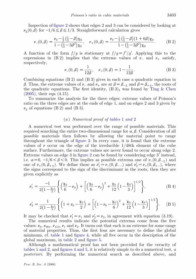
Figure 2. The irreducible 1/48th of the cube surface is defined by the isosceles triangle with edges 1,2 and 3. The vertices opposite these edges correspond to, nZ111, 110 and 001, respectively. Notethat the edge 30 is equivalent to 3 (which is used in appendix B).

0.25

0.20111

110

001

0.15H

0.10

0.05

00.6

0.4 0.20

00.2

0.40.6

0.8

n1

n2

Figure 1. The function H of equation (2.21) plotted versus n1 and n2 for the region of solid angledepicted in figure 2. Vertices nZ111, 110 and 001 are indicated. H vanishes at 111 and 001 and ispositive elsewhere, with maximum of 1/4 along nZ110 (face diagonals).

A. N. Norris3390

where HðnÞ is, see figure 1,

HðnÞZ ½ðn21n

22 Cn2

2n23 Cn2

3n21Þ2K3n2

1n22n

23�1=2: ð2:21Þ

3. Poisson’s ratio

We now consider the global extrema of nðn;mÞ over all directions n and m. Twomethods are used to derive the main results. The first uses general equations for astationary value of n in anisotropic media to obtain a single equation which mustbe satisfied if the stationary value lies in the interior of the triangle in figure 2. Itis shown that this condition, which is independent of material parameters, is notsatisfied, and hence all stationary values of n in cubic materials lie on the edges ofthe triangle. This simplifies the problem considerably, and permits us to deduce

Proc. R. Soc. A (2006)

3391Poisson’s ratio in cubic materials

explicit relations for the stationary values. The second method, described inappendix B, confirms the first approach by a comprehensive numerical test of allpossible material parameters.

(a ) General conditions for stationary Poisson’s ratio

General conditions can be derived which must be satisfied in order thatPoisson’s ratio is stationary in anisotropic elastic materials (Norris submitted).These are

s 014 Z 0; 2ns 015Cs 025 Z 0; ð2nK1Þs 016Cs 026 Z 0; ð3:1Þ

where the stretch is in the 10 direction ðnÞ and 20 is in the lateral direction ðmÞ.The conditions may be obtained by considering the derivative of n with respect torotation of the pair ðn;mÞ about an arbitrary axis. Setting the derivatives to zeroyields the stationary conditions (3.1).

The only non-zero contributions to s 014, s015, s

025, s

016 and s 026 in a material of

cubic symmetry come from D. Thus, we may rewrite the conditions forstationary values of n in terms of D 0

14ZD 01123, etc. as

D 014 Z 0; 2nD 0

15CD 025 Z 0; ð2nK1ÞD 0

16CD 026 Z 0: ð3:2Þ

The first is automatically satisfied by virtue of the choice of the direction-m aseither of mG. Regardless of which is chosen,

D 014 ZDijklninjmCkmKl

Z rCrKn41

ðn21KlCÞðn2

1KlKÞC

n42

ðn22KlCÞðn2

2KlKÞC

n43

ðn23KlCÞðn2

3KlKÞ

� �

Z 0:

ð3:3Þ

The final identity may be derived by first splitting each term into partialfractions and using the following (cf. appendix A):

n41

n21KlG

Cn42

n22KlG

Cn43

n23KlG

Z 1: ð3:4Þ

With no loss in generality, consider the specific case of mZma, lZla, whereaZG, and in either case, bZKa. It may be shown without much difficulty(appendix B) that rGO0 for n in the interior of the triangle of figure 2. It thenfollows that inside the triangle,

D 015

rbZ

D 016

raZ 1;

D 025

rbZ

la

laKlb;

D 026

raZ

la

laKlbK2: ð3:5Þ

These identities may be obtained using partial fraction identities similar to thosein equations (3.3) and (3.4). Equations (3.2)2 and (3.2)3 can be rewritten

D 015 D 0

25

D 016 D 0

26KD 016

" #2n

1

!Z

0

0

!: ð3:6Þ

Proc. R. Soc. A (2006)

A. N. Norris3392

However, using (3.5), the determinant of the matrix is

D 015D

026KðD 0

15CD 025ÞD 0

16 ZK3rCrK; ð3:7Þwhich is non-zero inside the triangle of figure 2. This gives us the importantresult: there are no stationary values of n inside the triangle of figure 2. Hence,the only possible stationary values are on the edges.

(b ) Stationary conditions on the triangle edges

The analysis above for the three conditions (3.2) is not valid on the triangleedges in figure 2, because the quantities rG become zero and careful limits mustbe taken. We avoid this route by considering the conditions (3.2) afresh for ndirected along the three edges. We find, as before, that D 0

14Z0 on the threeedges, so that (3.2)1 always holds. Of the remaining two conditions, one is alwayssatisfied, and imposing the other condition gives the answer sought.

The direction-n can be parametrized along each edge with a single variable.Thus, nZ1p0, 0%p%1, on edge 1. Similarly, edges 2 and 3 are together coveredby nZ11p, with 0%p!N. In each case, we also need to consider the twopossible values of m, which we proceed to do, focusing on the conditions (3.2)2and (3.2)3.

(i) Edge 1: nZ1p0, 0%p%1 and mZp�10 or 001

For mZp�10, we find that D 015ZD 0

25Z0 and D 016ZKD 0

26ZpKp3. Hence,equation (3.2)2 is automatically satisfied, while equation (3.2)3 becomes

ðnK1ÞðpKp3ÞZ 0: ð3:8Þ

Conversely, for mZ001 it turns out that D 016ZD 0

26Z0 and D 015ZKD 0

25ZpKp3.In this case, the only non-trivial equation from equations (3.2) is the second one,

nðpKp3ÞZ 0: ð3:9ÞApart from the specific cases nZ0 or 1, equations (3.8) and (3.9) imply thatstationary values of n occur only at the end points pZ0 and 1. Thus, nð001Þ,nð110; 1�10Þ and nð110; 001Þ are potential candidates for global extrema of n.

(ii) Edges 2 and 3: nZ11p, 0%p!N and mZ1�10

Proceeding as before, we find that D 016ZD 0

26Z0, D 015Z

ffiffiffi2

ppð1Kp2Þ=ð2Cp2Þ2

and D 025Zp=½

ffiffiffi2

pð2Cp2Þ�. Hence, equation (3.2)3 is automatically satisfied, while

equation (3.2)2 becomes

p½ð1K4nÞp2C2C4n�Z 0: ð3:10Þ

The zero pZ0 corresponds to nZ110 which was considered above. Thus, allthree conditions (3.2) are met if p is such that

p2 Z ðnC1=2Þ=ðnK1=4Þ: ð3:11Þ

Proc. R. Soc. A (2006)

3393Poisson’s ratio in cubic materials

Further progress is made using the representation of equation (2.13) combinedwith the limiting values of D which can be easily evaluated. We find

E111

E11p

Z 1C1

3

1Kp2

2Cp2

� �2E111c; ð3:12aÞ

nð11p; 1�10Þ E111

E11p

Z n111K1

6

1Kp2

2Cp2

� �E111c: ð3:12bÞ

Substituting for p2 from equation (3.11) into (3.12) gives two coupled equationsfor E11p and nð11p; 1�10Þ:

1

E11p

Z1

E111

Cc

48n2;

n

E11p

Zn111

E111

Cc

24n: ð3:13Þ

Eliminating E11p yields a single equation for possible stationary values ofnð11p; 1�10Þ,

n2Knn111K1

48E111cZ 0: ð3:14Þ

We will return to this after considering the other possible m vector.

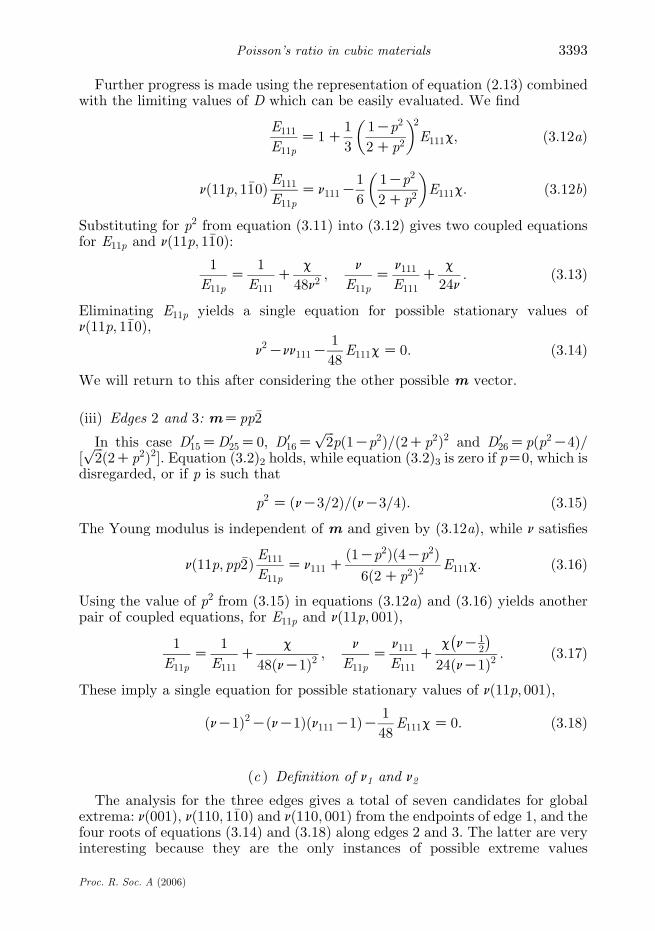
(iii) Edges 2 and 3: mZpp�2

In this case D 015ZD 0

25Z0, D 016Z

ffiffiffi2

ppð1Kp2Þ=ð2Cp2Þ2 and D 0

26Zpðp2K4Þ=½ffiffiffi2

pð2Cp2Þ2�. Equation (3.2)2 holds, while equation (3.2)3 is zero if pZ0, which is

disregarded, or if p is such that

p2 Z ðnK3=2Þ=ðnK3=4Þ: ð3:15ÞThe Young modulus is independent of m and given by (3.12a), while n satisfies

nð11p; pp�2Þ E111

E11p

Z n111Cð1Kp2Þð4Kp2Þ

6ð2Cp2Þ2E111c: ð3:16Þ

Using the value of p2 from (3.15) in equations (3.12a) and (3.16) yields anotherpair of coupled equations, for E11p and nð11p; 001Þ,

1

E11p

Z1

E111

Cc

48ðnK1Þ2;

n

E11p

Zn111

E111

Cc nK1

2

� �24ðnK1Þ2

: ð3:17Þ

These imply a single equation for possible stationary values of nð11p; 001Þ,

ðnK1Þ2KðnK1Þðn111K1ÞK 1

48E111cZ 0: ð3:18Þ

(c ) Definition of n1 and n2

The analysis for the three edges gives a total of seven candidates for globalextrema: nð001Þ, nð110; 1�10Þ and nð110; 001Þ from the endpoints of edge 1, and thefour roots of equations (3.14) and (3.18) along edges 2 and 3. The latter are veryinteresting because they are the only instances of possible extreme values

Proc. R. Soc. A (2006)

A. N. Norris3394

associated with directions other than the principal directions of the cube (axes,face diagonals). Results below will show that five of the seven candidates areglobal extrema, depending on the material properties. These are nð001Þ,nð110; 1�10Þ, nð110; 001Þ and the following two distinct roots of equations (3.14)and (3.18), respectively,

n1 h1

2n111K

1

2

ffiffiffiffiffiffiffiffiffiffiffiffiffiffiffiffiffiffiffiffiffiffiffiffiffiffiffiffiffiffiffiffiffiffiffiffiffiffiffiffiffiffiffiffiffiffiffiffiffiffiffiffiffiffiffiffiffin2111C

1

6ðn111C1Þ m1

m2

K1

� �s; ð3:19aÞ

n2 h1

2ðn111C1ÞC 1

2

ffiffiffiffiffiffiffiffiffiffiffiffiffiffiffiffiffiffiffiffiffiffiffiffiffiffiffiffiffiffiffiffiffiffiffiffiffiffiffiffiffiffiffiffiffiffiffiffiffiffiffiffiffiffiffiffiffiffiffiffiffiffiffiffiffiffiffiffiffiffiðn111K1Þ2 C 1

6ðn111C1Þ m1

m2

K1

� �s: ð3:19bÞ

The quantity E111c has been replaced to emphasize the dependence upon the twoparameters n111 and the anisotropy ratio m1=m2. The associated directions followfrom equations (3.11) and (3.15),

n1 Z nð11p1; 1�10Þ; p1 Zn1 C1=2

n1K1=4

� �1=2

; ð3:20aÞ

n2 Z nð11p2; p2p2�2Þ; p2 Zn2K3=2

n2K3=4

� �1=2

: ð3:20bÞ

A complete analysis is provided in appendix B. At this stage, we note that n1 isidentical to the minimum value of n deduced by Ting & Chen (2005), i.e. eqns(4.13) and (4.15) of their paper, with the minus sign taken in eqn (4.13).

4. Material properties in terms of Poisson’s ratios

Results for the global extrema are presented after we introduce several quantities.

(a ) Non-dimensional parameters

It helps to characterize the Poisson’s ratio in terms of two non-dimensionalmaterial parameters which we select as n0 and c0, where

n0 Z3kK2m2

6kC2m2

; c0 ZmK12 KmK1

1

ð9kÞK1 Cð3m2ÞK1: ð4:1Þ

That is, n0ZKs12=s11 is the axial Poisson’s ratio nð001; $Þ, independent of theorthogonal direction, and c0Zc=s11 is the non-dimensional analogue of c. Thus,

nðn;mÞZn0K

12 c0Dðn;mÞ

1Kc0FðnÞ; ð4:2Þ

a form which shows clearly that n is negative (positive) for all directions if n0!0and c0O0 (n0O0 and c0!0). These conditions for cubic materials to becompletely auxetic (non-auxetic) were previously derived byTing&Barnett (2005).

Proc. R. Soc. A (2006)

3395Poisson’s ratio in cubic materials

The extreme values of the Poisson’s ratio for a given n are

nGðnÞZn0K

12 c0ðFGHÞ1Kc0F

; ð4:3Þ

where F is defined in (2.7) and H in (2.21). Thus, nC is the minimum (maximum)and nK the maximum (minimum) if c0O0 ðc0!0Þ, respectively.

The Poisson’s ratio is a function of the direction pair ðn;mÞ and the materialparameter pair ðn0;c0Þ, i.e. nZnðn;m; n0;c0Þ. The dependence upon n0 has aninteresting property: for any orthonormal triad,

nðn;m; n0;c0ÞCnðn; t; 1Kn0;c0ÞZ 1: ð4:4ÞThis follows from (4.2) and the identities (2.8). Result (4.4) will prove usefullater.

Several particular values of Poisson’s ratio have been introduced:n0Znð001;mÞ, n111Znð111;mÞ associated with the two directions 001 and111 for which n is independent of m. These are two vertices of the trianglein figure 2. At the third vertex (nZ110 along the face diagonals), we havenð110;mÞZm2

3n001Cð1Km23Þn1�10 where, in the notation of (Milstein & Huang

1979) n001hnð110; 001Þ and n1�10 hnð110; 1�10Þ. Three of these four values ofPoisson’s ratio associated with principal directions can be global extrema, andthe fourth, n111 plays a central role in the definition of n1 and n2 of (3.19). Wetherefore consider them in terms of the non-dimensional parameters n0 and c0,

n111 Zn0K

16 c0

1K13 c0

; n001 Zn0

1K14 c0

; n1�10 Zn0K

14 c0

1K14 c0

: ð4:5Þ

We return to n1 and n2 later.

(b ) Positive definiteness and Poisson’s ratios

In order to summarize the global extrema of n, we first need to consider therange of possible material parameters. It may be shown that the requirements forthe strain energy to be positive definite: kO0, m2O0 and m1O0, can be expressedin terms of n0 and c0 as

K1!n0!1=2; c0!2ð1Cn0Þ: ð4:6ÞIt will become evident that the global extrema for n depend most simply on thetwo values for n along a face diagonal: n001 and n1�10. The constraints (4.6)become

K1!n1�10!1; K12 ð1Kn1�10Þ!n001!1Kn1�10; ð4:7Þ

which define the interior of a triangle in the n001; n1�10 plane, see figure 3. Thisfigure also indicates the lines n0Z0 and c0Z0 (isotropy). It may be checked thatthe four quantities fn0; n111; n001; n1�10g are different as long c0s0, with theexception of n001 and n0 which are distinct if n0c0s0. Consideration of the fourpossibilities yields the ordering

0!n001!n0!n111!n1�10!1 for n0O0; c0!0; ð4:8aÞ

K1!n0!n001!n111!n1�10!0 for n0!0; c0!0; ð4:8bÞ

Proc. R. Soc. A (2006)

–1.5 –1.0 –0.5 0 0.5 1.0 1.5 2.0 2.5–2.0

–1.5

–1.0

–0.5

0

0.5

1.0

1.5

n 001

m1=0

n0=0

m2=0

c0=0

m2=•

m1=•

k =•

k =0

b

a

c

d

n110_

Figure 3. The interior of the triangle in the n001; n1�10 plane represents the entirety of possible cubicmaterials with positive definite strain energy. The vertices correspond to kZ0, m1Z0 and m2Z0,as indicated. The edges of the triangle opposite the vertices are the limiting cases in which kK1, mK1

1

and mK12 vanish, respectively. The dashed curves correspond to n0Z0 (vertical) and c0Z0

(diagonal) and the regions a, b, c and d defined by these lines coincide with the four cases inequation (4.8), respectively.

A. N. Norris3396

K1!n1�10!n111!n001!n0!0 for n0!0; c0O0; ð4:8cÞ

0!n1�10!n111!n0!n001!2 for n0O0; c0O0: ð4:8dÞ

Note that n111 is never a maximum or minimum. We will see below that (4.8a) isthe only case for which the extreme values coincide with the global extrema for n.This is one of the reasons the classification of the extrema for n is relativelycomplicated, requiring that we identify several distinct values. In particular, theglobal extrema depend upon more than sgn n0 and sgn c0, but are bestcharacterized by the two independent non-dimensional parameters n001 and n1�10.

We are now ready to define the global extrema.

5. Minimum and maximum Poisson’s ratio

Tables 1 and 2 list the values of the global minimum nmin and the globalmaximum nmax, respectively, for all possible combinations of elastic parameters.For table 1, nð001Þ, n001 and n1�10 are defined in (4.5), and n1 and p1 are defined in(3.19a) and (3.20a). For table 2, n2 and p2 are defined in (3.19b) and (3.20b). Nosecond condition is necessary to define the region for case e, which is clear fromfigure 5. The data in tables 1 and 2 are illustrated in figures 4 and 5, respectively,which define the global extrema for every point in the interior of the triangle

Proc. R. Soc. A (2006)

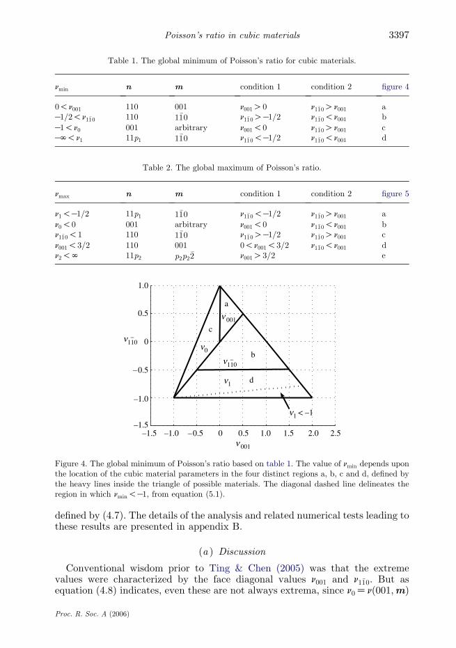
Table 1. The global minimum of Poisson’s ratio for cubic materials.

nmin n m condition 1 condition 2 figure 4

0!n001 110 001 n001O0 n1�10On001 aK1=2!n1�10 110 1�10 n1�10OK1=2 n1�10!n001 b

K1!n0 001 arbitrary n001!0 n1�10On001 cKN!n1 11p1 1�10 n1�10!K1=2 n1�10!n001 d

Table 2. The global maximum of Poisson’s ratio.

nmax n m condition 1 condition 2 figure 5

n1!K1=2 11p1 1�10 n1�10!K1=2 n1�10On001 a

n0!0 001 arbitrary n001!0 n1�10!n001 bn1�10!1 110 1�10 n1�10OK1=2 n1�10On001 c

n001!3=2 110 001 0!n001!3=2 n1�10!n001 dn2!N 11p2 p2p2�2 n001O3=2 e

n1 < –1

a

d

c

b

–1.5 –1.0 –0.5 0 0.5 1.0 1.5 2.0 2.5–1.5

–1.0

–0.5

0

0.5

1.0

n 001

n 001

n110_

n110_

n1

n0

Figure 4. The global minimum of Poisson’s ratio based on table 1. The value of nmin depends uponthe location of the cubic material parameters in the four distinct regions a, b, c and d, defined bythe heavy lines inside the triangle of possible materials. The diagonal dashed line delineates theregion in which nmin!K1, from equation (5.1).

3397Poisson’s ratio in cubic materials

defined by (4.7). The details of the analysis and related numerical tests leading tothese results are presented in appendix B.

(a ) Discussion

Conventional wisdom prior to Ting & Chen (2005) was that the extremevalues were characterized by the face diagonal values n001 and n1�10. But asequation (4.8) indicates, even these are not always extrema, since n0Znð001;mÞ

Proc. R. Soc. A (2006)

n 2 > 2

a

b

c

d

e

–1.5

–1.0

–0.5

0

0.5

1.0

n110_

n110_

–1.5 –1.0 –0.5 0 0.5 1.0 1.5 2.0 2.5n 001

n 001n 0n 1

n 2

Figure 5. The global maximum of Poisson’s ratio based on table 2. The value of nmax depends uponthe location of ðn001; n1�10Þ in five distinct regions defined by the heavy lines. The dashed linedelineates the (small) region in which nmaxO2, from equation (5.1).

A. N. Norris3398

can be maximum or minimum under appropriate circumstances (equations (4.8c)and (4.8d), respectively). The extreme values in equation (4.8) are all boundedby the limits of the triangle in figure 3. Specifically, they limit the Poisson’s ratioto lie between K1 and 2. Ting & Chen (2005) showed by explicit demonstrationthat this is not the case, and that values less than K1 and larger than 2 arefeasible, and remarkably, no lower or upper limits exist for n.

The Ting & Chen ‘effect’ occurs in figure 4 in the region, where nminZn1 and infigure 5 in the region nmaxZn2. Using equation (3.19a), we can determine thatnmin is strictly less than K1 if ðm1=m2K1ÞO24. Similarly, equation (3.19b)implies that nmax is strictly greater than 2 if ðm1=m2K1Þðn111C1ÞO24ð2Kn111Þ.By converting these inequalities, we deduce

nmin!K1 5 m2!m1

255 n001K13n1�10O12; ð5:1aÞ

nmaxO2 5 m2!25

m1

C16

k

!K1

5 13n001Kn1�10O24 : ð5:1bÞ

The two sub-regions defined by the n001, n1�10 inequalities are depicted in figures 4and 5. They define neighbourhoods of the m2Z0 vertex, i.e. ðn001; n1�10ÞZð2;K1Þ,where the extreme values of n can achieve arbitrarily large positive and negativevalues. The condition for nmin!K1 is independent of the bulk modulus k. Thus,the occurrence of negative values of n less than K1 does not necessarily implythat relatively large positive values (greater than 2) also occur, but the converseis true. This is simply a consequence of the fact that the dashed region near thetip m2Z0 in figure 5 is contained entirely within the dashed region of figure 4.

These results indicate that the necessary and sufficient condition for theoccurrence of large extrema for n is that m2 is much less than either m1 or k. m2 iseither the maximum or minimum of G, and it is associated with directions pairs

Proc. R. Soc. A (2006)

Table 3. Properties of the 11 materials of cubic symmetry in figure 6 with n1�10!K1=2. (Theboldfaced numbers indicate nmin and nmax. Unless otherwise noted the data are from Landolt &Bornstein (1992). G&S indicates Gunton & Saunders (1975).)

material n001 n1�10 n1 p1 n2 p2 m1=m2

b-brass (Musgrave 2003) 1.29 K0.52 K0.52 0.15 8.5Li 1.29 K0.53 K0.54 0.21 8.8AlNi (at 63.2% Ni and at 273 K) 1.28 K0.55 K0.55 0.25 9.1CuAlNi (Cu14% Al4.1% Ni) 1.37 K0.58 K0.59 0.32 10.2CuAlNi (Cu14.5% Al3.15% Ni) 1.41 K0.63 K0.66 0.42 12.1CuAlNi 1.47 K0.65 K0.69 0.45 13.1AlNi (at 60% Ni and at 273 K) 1.53 K0.68 K0.74 0.50 1.53 0.18 15.0InTl (at 27% Tl, 290 K) (G&S) 1.75 K0.78 K0.98 0.62 1.89 0.59 24.0InTl (at 28.13% Tl) 1.78 K0.81 K1.08 0.66 2.00 0.63 28.6InTl (at 25% Tl) 1.82 K0.84 K1.21 0.70 2.14 0.68 34.5InTl (at 27% Tl, 200 K) (G&S) 1.93 K0.94 K2.10 0.83 3.01 0.82 90.9

3399Poisson’s ratio in cubic materials

along orthogonal face diagonals, m2ZGð110; 1�10Þ. Hence, the Ting & Chen effectrequires that this shear modulus is much less than m1ZGð001;mÞ, and much lessthan the bulk modulus k. In the limit of very small m2, equations (3.19)

give n1;2zHffiffiffiffiffiffiffiffiffiffiffiffiffiffiffiffiffiffiffiffiffiffiffiffiffiffiffiffiffiffiffiffiffiffiffiffiffiffiffiffiðn111C1Þm1=ð24m2Þ

p. Ting (2004) found that the extreme values are

nzGffiffiffiffiffiffiffiffiffiffiffiffiffiffiffiffi3=ð16dÞ

pCOð1Þ for small values of their parameter d. In current notation,

this is dZ9=½1CE111c�, and replacing E111c the two theories are seen to agree.The implications of small m2 for Young’s modulus are apparent. Thus,

Emin=EmaxZOðm2=m1Þ, and equation (2.13)1 indicates that EðnÞ is smalleverywhere except near the 111-direction, at which it reaches a sharply peakedmaximum. Cazzani & Rovati (2003) provide numerical examples illustrating thedirectional variation of E for a range of cubic materials, some of which areconsidered below. Their three-dimensional plots of EðnÞ for materials with verylarge values of m1=m2 (see table 3 below) look like very sharp starfish. Although,the directions at which n1 and n2 are large in magnitude are close to the 111-direction, the value of E in the stationary directions can be quite different fromE111. The precise values of the Young modulus, E11p1 and E11p at the associatedstretch directions are given by

E111

E11p1

Cn111

n1Z 2;

E111

E11p2

Cn111K1

n2K1Z 2: ð5:2Þ

These identities, which follow from equations (3.13) and (3.17), respectively,indicate that if n1 or n2 become large in magnitude then the second term in theleft member is negligible. The associated value of the Young modulus isapproximately one half of the value in the 111-direction and consequently largevalues of jnj occur in directions at which Ezð1=2ÞE111. Such directions, by theirnature, are close to 111.

The appearance of n1 in both figures 4 and 5 is not surprising if oneconsiders that n001, n1�10 and n0 also occur in both the minimum and maximum.It can be checked that in the region where n1 is the maximum value infigure 5, it satisfiesK1!n1!K1=2. In fact, it is very close to but not equal to

Proc. R. Soc. A (2006)

n 1 <–1

nmin = n001

–1.0

–0.5

0

0.5

1.0

n110_

n001

n110_

–1.0 –0.5 0 0.5 1.0 1.5 2.0

n 1

n 0

Figure 6. The 44 materials considered are indicated by dots on the chart showing the nmin regions,cf. figure 4.

A. N. Norris3400

n1�10 in this region, and numerical results indicate that jn1Kn1�10j!4!10K4 inthis small sector.

What is special about the transition values in figures 4 and 5: n001Z3=2 andn1�10ZK1=2? Quite simply, they are the values of n1 and n2 as the stationarydirections n approach the face diagonal direction-110. Thus, n1 and n2 are boththe continuation of the face diagonal value n1�10, but on two different branches.See appendix B for further discussion.

(b ) Application to cubic materials

We conclude by considering elasticity data for 44 materials with cubicsymmetry, figure 6. The data are from Musgrave (2003) unless otherwisenoted. The 17 cubic materials in the region, where nminZn001 are as follows,with the coordinates ðn001; n1�10Þ for each: GeTeSnTe1 (mol% GeTeZ0)(0.01, 0.70), RbBr1 (0.06, 0.64), KI (0.06, 0.61), KBr (0.07, 0.59), KCl(0.07, 0.56), Nb1 (0.21, 0.61), AgCl (0.23, 0.61), KFl (0.12, 0.49), CsCl(0.14, 0.44), AgBr (0.26, 0.55), CsBr (0.16, 0.40), NaBr (0.15, 0.38), NaI(0.15, 0.38), NaCl (0.16, 0.37), CrV1 (Cr0.67 at.% V) (0.15, 0.35), CsI(0.18, 0.38), NaFl (0.17, 0.32). This lists them roughly in the order from topleft to lower right. Note that all the materials considered have positive n001.The 16 materials with nminZn001 also have nmaxZn1�10, so the coordinates ofthe above materials correspond to their extreme values of n. The extremevalues are also given by the coordinates in the region with nminZn1�10,nmaxZn001. The materials there are: Al (0.41, 0.27), diamond (0.12, 0.01), Si(0.36, 0.06), Ge (0.37, 0.02), GaSb (0.44, 0.03), InSb (0.53, 0.03), CuAu1

(0.73, 0.09), Fe (0.63, K0.06), Ni (0.64, K0.07), Au (0.88, K0.03), Ag

(0.82,K0.09), Cu (0.82,K0.14), a-brass (0.90,K0.21), Pb1 (1.02,K0.20),

Rb1 (1.15,K0.40), Cs1 (1.22,K0.46).

1Data from Landolt & Bornstein (1992), see also Cazzani & Rovati (2003).

Proc. R. Soc. A (2006)

3401Poisson’s ratio in cubic materials

Materials with n1�10!K1=2 are listed in table 3. These all lie within the regionwhere the minimum is n1, and of these, five materials are in the sub-region wherethe maximum is n2. Three materials are in the sub-regions with n1!K1 andn2O2. These indium thallium alloys of different composition and at differenttemperatures are close to the stability limit where they undergo a martensiticphase transition from face-centred cubic form to face-centred tetragonal. Thetransition is discussed by, for instance, Gunton & Saunders (1975), who alsoprovide data on another even more auxetic sample: InTl (at 27% Tl, 125 K). Thismaterial is so close to the m2Z0 vertex, with n001Z1:991, n1�10ZK0:997 andm1=m2Z1905 (!) that we do not include it in the table or the figure for being tooclose to the phase transition, or equivalently, too unstable (it has n1ZK7:92 andn2Z8:21).

We note that the stretch directions for the extremal values of n, defined bynZ11p1 and 11p2, are distinct. As the materials approach the m2Z0 vertex, thedirections coalesce as they tend towards the cube diagonal 111. The threematerials in table 3 with nmin!K1 and nmaxO2 are close to the incompressibilitylimit, the line kZN in figure 3. In this limit, the averaged Poisson’s ratio is�nðnÞZ1=2, and therefore those Poisson’s ratios which are independent of m tendto 1=2, i.e. n111Zn0Z1=2. Also, n001Cn1�10Z1 and n1Cn2Z1, with

n1 Z1

4K

1

4

ffiffiffiffiffiffim1

m2

r; n2 Z

3

4C

1

4

ffiffiffiffiffiffim1

m2

r; p1 Z p2 Z

ffiffiffiffiffiffiffiffiffiffiffiffiffiffiffiffiffiffiffiffi1K3

ffiffiffiffiffiffim2

m1

rs; k/N: ð5:3Þ

These are reasonable approximations for the last three materials in table 3,which clearly satisfy n1Cn2z1 and p1zp2.

6. Summary

Figures 4 and 5 along with tables 1 and 2 are the central results which summarizethe extreme values of Poisson’s ratio for all possible values of the elasticparameters for solids with positive strain energy and cubic material symmetry.The application of the related formulae to the materials in figure 6 shows thatvalues less than K1 and greater than C2 are associated with certain stretchdirections in some indium thallium alloys.

Discussions with Prof. T.C.T. Ting are appreciated.

Appendix A. Extreme values of D(n,m) for a given n

The extreme values of Dðn;mÞ as a function of m for a given direction-n can bedetermined using Lagrange multipliers l; r, and the generalized function

f ðmÞZDðn;mÞKljmj2K2rn$m: ðA 1Þ

Setting to zero, the partial derivatives of f with respect to m1, m2, m3, impliesthree equations, which may be solved to give

mZrn1

n21Kl

;rn2

n22Kl

;rn3

n23Kl

� �; ðA 2Þ

Proc. R. Soc. A (2006)

A. N. Norris3402

where l; r follow from the constraints n$mZ0 and jmj2Z1. These are,respectively, (2.16) and

n21

ðn21KlÞ2

Cn22

ðn22KlÞ2

Cn23

ðn23KlÞ2

" #r2 Z 1: ðA 3Þ

Equation (2.16) implies that l is a root of the quadratic (2.17) and (A 3) yieldsthe normalization factor r. These results are summarized in (2.18) and (2.19).

It may be easily checked that the function f is zero at the extremal values of D.But fZDKl, and hence the extreme values of Dðn;mÞ are simply the two rootsof the quadratic (2.17), 0%lK%lC%1=2. Note that the extreme values dependonly upon the invariants of the tensor M with components MijZDijklnknl .Although this is a second-order tensor and normally possesses three independent

invariants, one is trivially a constant: trMZ1. The others are, e.g. tr M2Zn41C

n42Cn4

3Z1K2FðnÞ (see equation (2.8)) and det MZn21n

22n

23.

The above formulation is valid as long as ðn21Kn2

2Þðn22Kn2

3Þðn23Kn2

1Þs0. For

instance, if n22Zn2

1, then lK; lCZmin;maxðn21; 3n

21n

23Þ. The m vector associated

with lZn21 is undefined, according to (A 2). However, by taking the limit n2

2/n21

it can be shown that m/Gð1;K1; 0Þ=ffiffiffi2

p. The other vector corresponding to

lZ3n21n

23 has no such singularity, and ismZGðn3; n3;K2n1Þ=

ffiffiffi2

p.

The identity (3.4) may be obtained by noting that each term can be split, e.g.n41=ðn2

1KlÞZn21Cl=ðn2

1KlÞ, then using the fundamental relation (2.16) with

n21Cn2

2Cn23Z1. Various other identities can be found, e.g.

n61

ðn21KlCÞðn2

1KlKÞC

n62

ðn22KlCÞðn2

1KlKÞC

n63

ðn23KlCÞðn2

1KlKÞZ 1: ðA 4Þ

Appendix B. Analysis

Here, we derive stationary conditions for directions n along the edges of thetriangle in figure 2 by direct analysis. Numerical tests are performed for theentire range of material parameters. The results are consistent with and reinforcethose of §3.

The limiting Poisson’s ratios of (4.3) are expressed nGðnÞhnGða; bÞ in terms oftwo numbers, where

n21 Z ð1CaÞ 1

3Kb

� �; n2

2 Z ð1KaÞ 1

3Kb

� �; n2

3 Z1

3C2b: ðB 1Þ

The range of ða; bÞ which needs to be considered is 0%a%1, ða=3ð3CaÞÞ%b%1=3, corresponding to the triangle in figure 2. This parametrization allowsquick numerical searching for global extreme values of n for a given cubic material.

We first consider the three edges as shown in figure 2 in turn. Edge 1 is definedby aZ1, 1=12%b%1=3. The limiting values are nKð1; bÞZn0=½1Kðð1=3ÞKbÞ!ðð1=3ÞC2bÞ2c0� and nCð1;bÞZ1KnKð1;bÞð1Kn0Þ=n0. The extreme valuesare obtained at the ends: nKð1; 1=12ÞZn001, nCð1; 1=12ÞZn1�10, nKð1; 1=3ÞZnCð1; 1=3ÞZn0. These possible global extreme values agree with those of §3.

Proc. R. Soc. A (2006)

3403Poisson’s ratio in cubic materials

Inspection of figure 2 shows that edges 2 and 3 can be considered by looking atnGð0; bÞ forK1=6%b%1=3. Straightforward calculation gives

nKð0;bÞZn0K

12

13Kb� �

c0

1K 13K3b2� �

c0

; nCð0; bÞZn0K

12

13Kb� �

ð1C6bÞc0

1K 13K3b2� �

c0

: ðB 2Þ

A function of the form f =g is stationary at f =gZ f 0=g 0. Applying this to theexpressions in (B 2) implies that the extreme values of nK and nC satisfy,respectively,

nKð0; bÞZ1

12b; nCð0;bÞZ 1K

1

12b: ðB 3Þ

Combining equations (B 2) and (B 3) gives in each case a quadratic equation inb. Thus, the extreme values of nK and nC are at bZbKG and bZbCG, the roots ofthe quadratic equations. The first identity, (B 3)1 was found by Ting & Chen(2005), their eqn (4.15).

To summarize the analysis for the three edges: extreme values of Poisson’sratio on the three edges are at the ends of edge 1, and on edges 2 and 3 given bynG of equations (B 2) and (B 3).

(a ) Numerical proof of tables 1 and 2

A numerical test was performed over the range of possible materials. Thisrequired searching the entire two-dimensional range for a; b. Consideration of allpossible materials then follows by allowing the material point to rangethroughout the triangle of figure 3. In every case, it is found that the extremevalues of n occur on the edge of the irreducible 1/48th element of the cubesurface. Furthermore, the extreme values are never found to occur along edge 2.Extreme values on edge 3 in figure 2 can be found by considering edge 30 instead,i.e. aZ0,K1=6!b!0. This implies as possible extrema one of nKð0; bKGÞ andone of nCð0;bCGÞ. We define these as n01ZnKð0;bKKÞ and n02ZnCð0; bCKÞ, wherethe signs correspond to the sign of the discriminant in the roots, then they aregiven explicitly as

n01 ZK1

2 1Kc0

3

� � c0

6Kn0

� C

c0

6Kn0

� 2C

c0

121K

c0

3

� � �1=2( ); ðB 4Þ

n02 Z1

2 1Kc0

3

� � 1Cn0Kc0

2

� C 1Kn0K

c0

6

� 2C

c0

121K

c0

3

� � �1=2( ): ðB 5Þ

It may be checked that n01Zn1 and n02Zn2, in agreement with equation (3.19).The numerical results indicate the potential extrema come from the five

values: n0, n001, n1�10, n1 and n2. It turns out that each is an extreme for some rangeof material properties. Thus, the first four are necessary to define the globalminimum, cf. table 1 and figure 4, while all five occur in the description of theglobal maximum, in table 2 and figure 5.

Although a mathematical proof has not been provided for the veracity oftables 1 and 2, and figures 4 and 5, it is relatively simple to do a numerical test, aposteriori. By performing the numerical search as described above, and

Proc. R. Soc. A (2006)

A. N. Norris3404

subtracting the extreme values of tables 1 and 2, one finds zero, or its numericalapproximant for all points in the interior of the triangle of possible materials,figure 2.

In order to further justify the results as presented, appendix Bb gives argumentsfor the occurrence of the special values K1/2 and 3/2 in figures 4 and 5.

(b ) Significance of K1/2 and 3/2

Suppose Poisson’s ratio is the same for two different pairs of directions:nðn;mÞZnðn�;m�Þ. The pairs ðn;mÞ and ðn�;m�Þ must satisfy, using (4.2),

Dðn;mÞKDðn�;m�ÞFðnÞKFðn�Þ Z 2n: ðB 6Þ

For instance, let n�Z110, m�Z001, so that nZn001. Equation (B 6) impliesthat the same Poisson’s ratio is achieved for directions ðn;mÞ satisfying

Dðn;mÞ2FðnÞK1=2

Z n001: ðB 7Þ

Note that this is independent of n0 and c0. We choose n001 specifically because ithas been viewed as the candidate for largest Poisson’s ratio, until Ting &Chen (2005). If it is not the largest, then there must be pairs ðn;mÞ other thanð110; 001Þ for which (B 7) holds. However, it may be shown using results from §2that the minimum of the left member in (B 7) is 3/2, and the minimum occurs atnZ110, as one might expect. This indicates that n001 must exceed 3/2 in orderfor the largest Poisson’s ratio to occur for n other than the face diagonal 110.

Returning to (B 6), let nZn1�10, then nðn;mÞZn1�10 if

12KDðn;mÞ2FðnÞK1

2

ZKn1�10: ðB 8Þ

Using equation (2.8) and the previous result, it can be shown that the minimumof the left member in (B 8) is 1/2, and the minimum is at nZ110. Hence, n1�10must be less than K1/2 in order for the smallest Poisson’s ratio to occur for nother than the face diagonal 110. These two results explain why the particularvalues n001Z3=2 and n1�10ZK1=2 appear in tables 1 and 2 and in figures 4 and 5.

References

Baughman, R. H., Shacklette, J. M., Zakhidov, A. A. & Stafstrom, S. 1998 Negative Poisson’sratios as a common feature of cubic metals. Nature 392, 362–365. (doi:10.1038/32842)

Boulanger, Ph. & Hayes, M. A. 1998 Poisson’s ratio for orthorhombic materials. J. Elasticity 50,87–89. (doi:10.1023/A:1007468812050)

Cazzani, A. & Rovati, M. 2003 Extrema of Young’s modulus for cubic and transversely isotropicsolids. Int. J. Solids Struct. 40, 1713–1744. (doi:10.1016/S0020-7683(02)00668-6)

Gunton, D. J. & Saunders, G. A. 1975 Stability limits on the Poisson ratio: application to amartensitic transformation. Proc. R. Soc. 343, 68–83.

Hayes, M. A. 1972 Connexions between the moduli for anisotropic elastic materials. J. Elasticity 2,135–141. (doi:10.1007/BF00046063)

Proc. R. Soc. A (2006)

3405Poisson’s ratio in cubic materials

Hayes, M. A. & Shuvalov, A. 1998 On the extreme values of Young’s modulus, the shear modulus,and Poisson’s ratio for cubic materials. J. Appl. Mech. ASME 65, 786–787.

He, Q. C. 2004 Characterization of the anisotropic materials capable of exhibiting an isotropic Youngor shear or area modulus. Int. J. Eng. Sci. 42, 2107–2118. (doi:10.1016/j.ijengsci.2004.04.009)

Landolt, H. H. & Bornstein, R. 1992 Numerical data and functional relationships in science andtechnology, III/29/a. Second and higher order elastic constants. Berlin: Springer.

Lempriere, B. M. 1968 Poisson’s ratio in orthotropic materials. AIAA J. 6, 2226–2227.Love, A. E. H. 1944 Treatise on the mathematical theory of elasticity. New York, NY: Dover.Milstein, F. & Huang, K. 1979 Existence of a negative Poisson ratio in fcc crystals. Phys. Rev. B

19, 2030–2033. (doi:10.1103/PhysRevB.19.2030)Musgrave, M. J. P. 2003 Crystal acoustics. New York, NY: Acoustical Society of America.Norris, A. N. Submitted. Extreme values of Poisson’s ratio and other engineering moduli in

anisotropic solids.Scott, N. H. 2000 An area modulus of elasticity: definition and properties. J. Elasticity 58, 269–275.

(doi:10.1023/A:1007675928019)Sirotin, Yu. I. & Shaskol’skaya, M. P. 1982 Fundamentals of crystal physics. Moscow: MIR.Thomson, W. 1856 Elements of a mathematical theory of elasticity. Phil. Trans. R. Soc. 146,

481–498.Ting, T. C. T. 2004 Very large Poisson’s ratio with a bounded transverse strain in anisotropic

elastic materials. J. Elasticity 77, 163–176. (doi:10.1007/s10659-005-2156-6)Ting, T. C. T. & Barnett, D. M. 2005 Negative Poisson’s ratios in anisotropic linear elastic media.

J. Appl. Mech. ASME 72, 929–931. (doi:10.1115/1.2042483)Ting, T. C. T. & Chen, T. 2005 Poisson’s ratio for anisotropic elastic materials can have no

bounds. Q. J. Mech. Appl. Math. 58, 73–82. (doi:10.1093/qjmamj/hbh021)Walpole, L. J. 1984 Fourth rank tensors of the thirty-two crystal classes: multiplication tables.

Proc. R. Soc. A391, 149–179.Walpole, L. J. 1986 The elastic shear moduli of a cubic crystal. J. Phys. D: Appl. Phys. 19, 457–462.

(doi:10.1088/0022-3727/19/3/014)

Proc. R. Soc. A (2006)