Point Cloud Data Filtering and Downsamplingusing Growing Neural Gas

Sergio Orts-Escolano Vicente Morell Jose Garcıa-Rodrıguez Miguel Cazorla

Abstract— 3D sensors provide valuable information for mo-bile robotic tasks like scene classification or object recognition,but these sensors often produce noisy data that makes impossi-ble applying classical keypoint detection and feature extractiontechniques. Therefore, noise removal and downsampling havebecome essential steps in 3D data processing. In this work, wepropose the use of a 3D filtering and downsampling techniquebased on a Growing Neural Gas (GNG) network. GNG methodis able to deal with outliers presents in the input data. Thesefeatures allows to represent 3D spaces, obtaining an inducedDelaunay Triangulation of the input space. Experiments showhow GNG method yields better input space adaptation to noisydata than other filtering and downsampling methods like VoxelGrid. It is also demonstrated how the state-of-the-art keypointdetectors improve their performance using filtered data withGNG network. Descriptors extracted on improved keypointsperform better matching in robotics applications as 3D sceneregistration.

I. INTRODUCTION

Historically, humans have the ability to recognize anenvironment they visited before based on the 3D model theyunconsciously build in their heads based on the differentperspectives of the scene. This 3D model is built with someextra information so that humans can extract relevant features[1] that will help in future experiences to recognize theenvironment and even possible present objects. This learningmethod has been transferred to mobile robotics field over theyears. So, most current approaches in scene understandingand visual recognition are based on the same principle:keypoint detection and feature extraction on the perceivedenvironment. Over the years most efforts in this area havebeen made towards feature extraction and keypoint detectionon information obtained by traditional image sensors [2],[3], existing a gap in feature-based approaches that use 3Dsensors as input devices. However, in recent years, the num-ber of research papers concerned with 3D data processinghas increased considerably due to the emergence of cheap3D sensors capable of providing a real time data streamand therefore enabling feature-based computation of threedimensional environment properties like curvature, gettingcloser to human learning processes.

The Kinect device1, the time-of-flight camera SR40002 or

Sergio Orts-Escolano and Jose Garcia-Rodriguez are with the Departmentof Computer Technology of the University of Alicante (email: {sorts,jgarcia}@dtic.ua.es).

Vicente Morell and Miguel Cazorla are with the Department of Scienceof the Computation and Artificial Intelligence Department of the Universityof Alicante (email: {vmorell, miguel}@dccia.ua.es).

1Kinect for XBox 360: http://www.xbox.com/kinect Microsoft2Time-of-Flight camera SR4000 http://www.mesa-

imaging.ch/prodview4k.php

the LMS-200 Sick laser3 mounted on a sweeping unit are ex-amples of these devices. Besides, providing 3D information,some of these devices like the Kinect sensor can also providecolor information of the observed scene. However, using 3Dinformation in order to perform visual recognition and sceneunderstanding is not an easy task. The data provided by thesedevices is often noisy and therefore classical approachesextended from 2D to 3D space do not work correctly. Thesame occurs to 3D methods applied historically on syntheticand noise-free data. Applying these methods to partial viewsthat contains noisy data and outliers produces bad keypointdetection and hence computed features does not containeffective descriptions. Consequently, in order to perform aneffective keypoint detection is needed to remove as muchnoise as possible keeping descriptive features as corners oredges.

Classical filtering techniques like median or mean havebeen widely used to filter noisy point clouds [4], [5] obtainedfrom 3D sensors like the ones previously mentioned. Themedian filter is one of the simplest and wide-spread filtersthat has been applied. It is efficient and simple to implementbut can remove noise only if the noisy pixels occupy less thanone half of the neighbourhood area. Moreover, it removesnoise but at the expense of smoothing corners and edges ofthe input data.

Another filtering technique frequently used in point cloudnoise removal is the Voxel Grid method. The Voxel Gridfiltering technique is based on the input space samplingusing a grid of 3D voxels to reduce the number of points.This technique has been traditionally used in the area ofcomputer graphics to subdivide the input space and reducethe number of points [6], [7]. The Voxel Grid methodpresents some drawbacks: sensitivity to noisy input spaces.Moreover, since all the points present will be approximated(i.e., downsampled) with their centroid it does not representthe underlying surface accurately.

More complex noise removal techniques from image pro-cessing [8] have been used also on point clouds: the Bilateralfiltering technique, [9] applied on depth maps obtained from3D sensors, allows to remove noise considering corners andedges using Gaussian functions and range kernels. However,Bilateral filtering is not able to deal with outliers in the inputpoint cloud.

Based on the Growing Neural Gas network [10] several au-thors proposed related approaches for surface reconstruction

3LMS-200 Sick laser: http://robots.mobilerobots.com/wiki/SICK LMS-200 Laser Rangefinder

Proceedings of International Joint Conference on Neural Networks, Dallas, Texas, USA, August 4-9, 2013

978-1-4673-6129-3/13/$31.00 ©2013 IEEE 60

applications [11], [12]. However, most of these contributionsdo not consider noisy data obtained from RGB-D camerasusing noise-free CAD models.

In this paper, we propose the use of a 3D filtering anddownsampling technique based on the GNG network. Bymeans of a competitive learning, it makes an adaptationof the reference vectors of the neurons as well as theinterconnection network among them, obtaining a mappingthat tries to preserve the topology of an input space. Besides,GNG method is able to deal with outliers in the inputdata. These features allow to represent 3D spaces, obtainingan induced Delaunay Triangulation of the input space veryuseful to easily obtain features like corners, edges and so on.Filtered point cloud produced by the GNG method is used asinput of many state-of-the-art 3D keypoint detectors in orderto demonstrate how the filtered and downsampled point cloudimproves keypoint detection and hence feature extraction andmatching in 3D registration methods. Proposed method iscompared with one state-of-the-art filtering techniques, theVoxel Grid method. Results presented in Section IV showhow the proposed method overperforms Voxel Grid methodin input space adaptation and noise removal. In Figure 1, itis shown a general system overview of the steps involved inthe 3D scene registration problem.

Capture PointCloud

Filtering andDownsampling

Keypointdetection

Featureextraction

FindCorrespondences Registration

Fig. 1. General system overview

In this work we focus on the processing of 3D informationprovided by the Kinect sensor. Experimental results showthat the random error of depth measurement increases withincreasing distance to the sensor, and ranges from a fewmillimeters up to about 4 cm at the maximum range of thesensor. More information about the accuracy and precisionof the Kinect device can be found in [13].

The rest of the paper is organized as follows: first, asection describing briefly the GNG algorithm is presented.In section III the state-of-the-art 3D keypoint detectors aredescribed. In section IV we present some experiments anddiscuss results obtained using our novel approach. Finally, insection V we give our conclusions and directions for futurework.

II. GNG ALGORITHM

With Growing Neural Gas (GNG) [10] method a growthprocess takes place from minimal network size and new unitsare inserted successively using a particular type of vectorquantization. To determine where to insert new units, localerror measures are gathered during the adaptation process andeach new unit is inserted near the unit which has the highestaccumulated error. At each adaptation step a connectionbetween the winner and the second-nearest unit is createdas dictated by the competitive Hebbian learning algorithm.

This is continued until an ending condition is fulfilled, as forexample evaluation of the optimal network topology or fixednumber of neurons. The network is specified as:

• A set N of nodes (neurons). Each neuron c ∈ N hasits associated reference vector wc ∈ Rd. The referencevectors can be regarded as positions in the input spaceof their corresponding neurons.

• A set of edges (connections) between pairs of neurons.These connections are not weighted and its purpose is todefine the topological structure. An edge aging schemeis used to remove connections that are invalid due tothe motion of the neuron during the adaptation process.

The GNG learning algorithm to map the network to theinput manifold is as follows:

1) Start with two neurons a and b at random positions wa

and wb in Rd.2) Generate at random an input pattern ξ according to the

data distribution P (ξ) of each input pattern.3) Find the nearest neuron (winner neuron) s1 and the

second nearest s2.4) Increase the age of all the edges emanating from s1.5) Add the squared distance between the input signal and

the winner neuron to a counter error of s1 such as:

�error(s1) = ‖ws1 − ξ‖2 (1)

6) Move the winner neuron s1 and its topological neigh-bors (neurons connected to s1) towards ξ by a learningstep εw and εn, respectively, of the total distance:

�ws1 = εw(ξ − ws1) (2)

�wsn = εn(ξ − wsn) (3)

For all direct neighbors n of s1.7) If s1 and s2 are connected by an edge, set the age of

this edge to 0. If it does not exist, create it.8) Remove the edges larger than amax . If this results

in isolated neurons (without emanating edges), removethem as well.

9) Every certain number λ of input patterns generated,insert a new neuron as follows:

• Determine the neuron q with the maximum accu-mulated error.

• Insert a new neuron r between q and its furtherneighbor f :

wr = 0.5(wq + wf ) (4)

• Insert new edges connecting the neuron r withneurons q and f , removing the old edge betweenq and f .

10) Decrease the error variables of neurons q and f mul-tiplying them with a consistent α. Initialize the errorvariable of r with the new value of the error variableof q and f .

11) Decrease all error variables by multiplying them witha constant γ.

61

12) If the stopping criterion is not yet achieved (in our casethe stopping criterion is the number of neurons), go tostep 2.

This method offers further benefits over simple noise re-moval and downsampling algorithms: due to the incrementaladaptation of the GNG, input space denoising and filteringis performed in such a way that only concise properties ofthe point cloud are reflected in the output representation.Moreover, the GNG method has been modified regard orig-inal version, considering also original point cloud colourinformation. Once GNG network has been adapted to theinput space and it has finished learning step, each neuron ofthe net takes colour information from nearest neighbours inthe original input space. Colour information of each neuronis calculated as the average of weighted values of the K-nearest neighbours, obtaining a interpolated value of thesurrounding point. Color values are weighted using Euclideandistance from input pattern to neuron reference vector. Inaddition, this search is considerably accelerated using a Kd-tree structure. Colour downsampling is performed to applykeypoint detectors and feature extractors that deal with colourinformation.

III. KEYPOINT DETECTORS/DESCRIPTORS

In this section, we present the state-of-the-art 3D keypointdetectors used to test and measure the improvement achievedusing GNG method to filter and downsample the input data.In addition, we describe main 3D descriptors and featurea correspondence matching method that we used in ourexperiments.

A. Keypoint detectors

First keypoint detector used is the widely known SIFT(Scale Invariant Feature Transform) [14] method. It performsa local pixel appearance analysis at different scales. SIFTfeatures are designed to be invariant to image scale and rota-tion. SIFT detector has been traditionally used in 2D imagebut it has been extended to 3D space. 3D implementation ofSIFT differs from original in the use of depth and curvatureas the intensity value. SIFT detector uses neighbourhood ateach point within a fixed-radius assigning its intensity as theGaussian weighted sum of the neighbours’ intensity valuesin order to archive the 4-dimensional difference of Gaussians(DoG) scale space. Then it detects local maxima in these 4DDoG scale space when the point value is greater than all itsneighbours.

Other keypoint detectors used are based on a classicalHarris 2D keypoint detector. In [15] a refined Harris detectoris presented in order to detect keypoints invariable to affinetransformations. 3D implementations of these Harris detec-tors [16] use surface normals of 3D points instead of 2Dgradient images. Harris detector and its variants, extendedfrom 2D keypoint detectors, have been tested using theproposed method in Section IV. All Harris variants havein common covariance matrix computation, but each variantmakes a different evaluation of the trace and the determinantof the covariance matrix. Noble’s variant corners detection

algorithm [17] evaluates the ratio between the determinantand the trace of the covariance matrix. Tomasi’s variant[18] performs eigenvalue decomposition over the covariancematrix using the smallest eigenvalue as keypoint score.Lowe’s variant performs in a similar way than Noble’s onebut evaluating the ratio between the determinant and thesquared trace of the covariance matrix. These small changesin the evaluation of the covariance matrix generate differentkeypoint detection as we will see in Section IV.

B. Descriptors

Once keypoints have been detected, it is necessary toextract a descriptor over these points. In the last few yearssome descriptors that take advantage of 3D information havebeen presented. In [19] a pure 3D descriptor called PointFeature Histograms (PFH) is presented. The goal of thePFH formulation is to encode the points k-neighborhoodgeometrical properties by generalizing the mean curvaturearound the point using a multi-dimensional histogram ofvalues. This highly dimensional hyperspace provides an in-formative signature for the feature representation, is invariantto the 6D pose of the underlying surface, and copes verywell with different sampling densities or noise levels presentin the neighbourhood. A PFH representation is based onthe relationships between the points in the k-neighborhoodand their estimated surface normals. Briefly, it attempts tocapture as best as possible the sampled surface variations byconsidering all the interactions between the directions of theestimated normals.

A simplification of the descriptor described above ispresented as Fast Point Feature Histograms (FPFH) [20] andis based on a histogram of the differences of angles betweenthe normals of the neighbour points. This method is a fastrefinement of the Point Feature Histogram (PFH) that com-putes its own normal directions and it represents all the pairpoint normal diferences instead of the subset of these pairswhich includes the keypoint. It reduces the computationalcomplexity of the PFH algorithm from O(nk2) to O(nk).

In addition, we used another descriptor called Signatureof Histograms of OrienTations (SHOT) [21], which is basedon obtaining a repeatable local reference frame using theeigenvalue decomposition around an input point. Given thisreference frame, a spherical grid centered on the point dividesthe neighbourhood so that in each grid bin a weighted his-togram of normals is obtained. The descriptor concatenatesall such histograms into the final signature. There is alsoa color version (CSHOT) proposed in [22] that adds colorinformation.

C. Feature matching

Correspondences between features or feature matchingmethods are commonly based on the euclidean distancesbetween feature descriptors. Moreover, a rejection step isnecessary in order to remove false positives from the previousstep. One of the most used method to check the transfor-mation between pairs of matched correspondences is basedon the RANSAC (RANdom SAmple Consensus) algorithm

62

[23]. It is an iterative method that estimates the parametersof a mathematical model from a set of observed data whichcontains outliers. In our case, we used this method to searcha 3D transformation (our model) which best explain thedata (matches between 3D features). At each iteration of thealgorithm, a subset of data elements (matches) is randomlyselected. These elements are considered as inliers and amodel (3D transformation) is fitted to those elements. Therest of the data is then tested against the fitted model andincluded as inliers if its error is below a given threshold.If the estimated model is reasonably good (its error is lowenough and it has enough matches), it is considered as a goodsolution. This process is repeated a number of iterations andthe best solution is returned.

IV. EXPERIMENTATION

We performed different experiments on indoor scenes toevaluate the effectiveness and robustness of the proposedmethod. First, a normal estimation method is computed inorder to show how simple features like estimated normals areconsiderably affected by noisy data. Secondly, accurate inputspace adaptation capabilities of the GNG method are showedcalculating the Mean Square Error (MSE) of filtered pointclouds regard their ground truth. Due to the impossibilityof obtaining ground truth data from the Kinect Device, theexperiment is performed using synthetic CAD models anddata obtained from a simulated Kinect sensor. Finally, theproposed method is applied to 3D scene registration to showhow keypoint detection methods are improved obtainingmore accurate transformations. 3D scene registration is per-formed on a dataset comprised of 90 overlapped partial viewsof a room. Partial views are rotated 4 degrees in order tocover 360 degrees of the scene. Partial views were capturedusing the Kinect device mounted in a robotic arm with theaim of knowing the ground truth transformation. Experimentsimplementation, 3D data management (data structures) andtheir visualization have been developed using the PCL4

library.

A. Improving normal estimationNormal estimation methods based on the analysis of the

eigenvectors and eigenvalues of a covariance matrix createdfrom the nearest neighbours are very sensitive to noisy data.Therefore, in the first experiment, we computed normals onraw and filtered point clouds in order to demonstrate how asimple 3D feature like normal or curvature estimation canbe affected by the presence of noise and how the proposedmethod improves normal estimation producing more stablenormals.

In Figure 2 it is visually explained the effect causedby normal estimation on noisy data. Normal estimation iscomputed on the original and filtered point cloud using thesame radius search: rs = 0.1 (meters).

In Figure 3 can be observed how more stable normals areestimated using filtered point cloud produced by the GNG

4The Point Cloud Library (or PCL) is a large scale, open project [24] for2D/3D image and point cloud processing.

Fig. 2. Noise causes error in the estimated normal

method. 20, 000 neurons and 1, 000 patterns are used asconfiguration parameters for the GNG method in the filteredpoint cloud showed in Figure 3 (Right).

B. Filtering quality: input space adaptation

In this experiment we demonstrated how the GNG methodyields better input space adaptation to noisy data than otherfiltering and downsampling methods like Voxel Grid. In orderto perform the experiment, ground truth data is requiredto calculate the MSE error regarding original data. As theKinect device does not provide ground truth information,synthetic CAD models and data obtained from a simulatedKinect sensor are used as ground truth. For simulatinga Kinect sensor and obtaining ground truth data, Blensorsoftware [25] has been used. It allows us to generate syntheticscenes and to obtain partial views of the generated scene asif a Kinect device was used. The main advantage of thissoftware is that it provides ground truth. In Figure 4 can beseen a synthetic scene generated using Blensor. On the leftside it is shown the ground truth scene without noise and inthe right side it is shown the partial view of the scene asif a Kinect device had captured it. Added noise is simulatedusing a Gaussian distribution with different deviation factors.

To perform this experiment, we calculated the MSE ofthe filtered point cloud with Voxel Grid and with the GNGmethod respect to the ground truth. The MSE is used tomeasure the filtered point cloud error relative to the groundtruth and therefore it is a quantitative measure of the accuracyof the filtered point cloud. MSE is expressed in meters. VoxelGrid method presents some drawbacks as it does not allowspecifying a fixed number of points, as the number of pointsis given by the voxel size used for building the grid. Weforced the convergence to an approximate number in ourexperiments, making it comparison fairer. By contrast, theGNG neural network allows us to specify the exact numberof end points that represent the input space. The experimentdemonstrates the accuracy of the representation generatedby the GNG network structure compared with Voxel Gridmethod.

Table I shows the adaptation MSE for different modelsand scenes using the GNG and the Voxel Grid method.On the top of the Table I, adaptation MSE is calculatedfor partial views obtained from a simulated Kinect sensor(meters) while in the bottom is calculated for syntheticCAD models (millimetres). Different levels of added noiseσ are applied to the ground truth data. Results presentedin Table I shows how the GNG method provides a lowermean error and therefore better adaptation to the original

63

Fig. 3. Normal estimation comparison. Left: Normal estimation on raw point cloud. Right: Normal estimation on filtered point cloud produced by theGNG method

Fig. 4. Synthetic scene. Left: Ground truth without noise. Right: simulated Kinect view with added noise: σ = 0.5

TABLE IINPUT SPACE ADAPTATION MSE FOR DIFFERENT MODELS. VOXEL GRID

VERSUS GNG.

simulated Kinect VG 5000 VG 10000 GNG 5000 250λ GNG 10000 500λscene 1 σ = 0.15 0.0067 0.0064 0.0017 0.0022scene 1 σ = 0.25 0.0197 0.0181 0.0053 0.0065scene 1 σ = 0.40 0.0475 0.0430 0.0156 0.0185scene 2 σ = 0.15 0.0053 0.0051 0.0013 0.0017scene 2 σ = 0.25 0.0148 0.0135 0.0041 0.0051scene 2 σ = 0.40 0.0372 0.0336 0.0122 0.0143

CAD model VG 5000 VG 10000 GNG 5000 250λ GNG 10000 500λmodel 1 σ = 0.15 0.0643 0.0641 0.0684 0.0559model 1 σ = 0.25 0.0981 0.0994 0.0768 0.0642model 1 σ = 0.40 0.2037 0.2276 0.0903 0.0924model 2 σ = 0.15 0.1540 0.1504 0.1756 0.1209model 2 σ = 0.25 0.3055 0.3227 0.1938 0.1430model 2 σ = 0.40 0.8259 0.8895 0.2346 0.2122

input space, maintaining a better quality of representation inareas with a high degree of curvature and removing the noise

generated by the sensor. The Voxel Grid method filters all thepoints present approximating (i.e., downsampling) them withtheir centroid, it does not represent the underlying surfaceaccurately causing a worse adaptation. Experiments wereperformed with a fixed number of points, and in the caseof GNG it was tested with different number of input signalsλ generated by iteration, and different number of neurons,obtaining better results with a higher number of adjustmentswith the sacrifice of higher computation times. In Figure 5can be visually observed adaptation MSE presented in tableI for model 1. Voxel Grid output representations does notaccurately fit input space, smoothing information in the edgesand corners. From Table I we can observe that for used CADmodels 10, 000 neurons are needed to represent accuratelythe input space, since that kind of models have more points.However for synthetic scenes are only needed 5, 000 neuronsto represent the input space due to resolution of the input

64

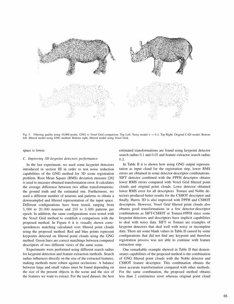
Fig. 5. Filtering quality using 10,000 points. GNG vs Voxel Grid comparison. Top Left: Noisy model σ = 0.4. Top Right: Original CAD model. Bottomleft: filtered model using GNG method. Bottom right: filtered model using Voxel Grid.

space is lower.

C. Improving 3D keypoint detectors performance

In the last experiment, we used some keypoint detectorsintroduced in section III in order to test noise reductioncapabilities of the GNG method for 3D scene registrationproblem. Root Mean Square (RMS) deviation measure [26]is used to measure obtained transformation error. It calculatesthe average difference between two affine transformations:the ground truth and the estimated one. Furthermore, weused a different number of neurons and patterns to obtain adownsampled and filtered representation of the input space.Different configurations have been tested, ranging from5, 000 to 20, 000 neurons and 250 to 2, 000 patterns perepoch. In addition, the same configurations were tested withthe Voxel Grid method to establish a comparison with theproposed method. In Figure 6 it is visually shown corre-spondences matching calculated over filtered point cloudsusing the proposed method. Red and blue points representkeypoints detected on filtered point clouds using the GNGmethod. Green lines are correct matchings between computeddescriptors of two different views of the same scene.

Experiments were performed using different search radiusfor keypoint detection and feature extraction methods. Searchradius influences directly on the size of the extracted features,making methods more robust against occlusions. A balancebetween large and small values must be found depending onthe size of the present objects in the scene and the size ofthe features we want to extract. For the used dataset, the best

estimated transformations are found using keypoint detectorsearch radius 0.1 and 0.05 and feature extractor search radius0.2.

In Table II it is shown how using GNG output represen-tation as input cloud for the registration step, lower RMSerrors are obtained in some detector-descriptor combinations.SIFT detector combined with the FPFH descriptor obtainslower RMS errors compared with Voxel Grid filtered pointclouds and original point clouds. Lowe detector obtainedlower RMS error for all descriptors. Tomasi and Noble de-tectors produced better results for the CSHOT descriptor andfinally, Harris 3D is also improved with FPFH and CSHOTdescriptors. However, Voxel Grid filtered point clouds alsoobtains good transformations in a few detector-descriptorcombinations as SIFT-CSHOT or Tomasi-FPFH since somekeypoint detectors and descriptors have implicit capabilitiesto deal with noisy data. SIFT or Tomasi are examples ofkeypoint detectors that deal well with noisy or incompletedata. There are some blank values in Table II caused by someconfigurations that did not find any keypoint and thereforeregistration process was not able to continue with featureextraction step.

One remarkable example showed in Table II that demon-strates capabilities of the proposed method is the combinationof GNG filtered point clouds with the Noble detector andCSHOT feature descriptor. This combination obtains themost accurate transformation compared with other methods.For the same combination, the proposed method obtainsless than 2 centimetres error whereas original point cloud

65

Fig. 6. Registration example done with the Lowe keypoint detector and the FPFH descriptor using a GNG representation with 20000 neurons.

TABLE IIRMS DEVIATION ERROR IN METERS OBTAINED USING DIFFERENT DETECTOR-DESCRIPTOR COMBINATIONS. COMBINATIONS ARE COMPUTED ON THE

ORIGINAL POINT CLOUD (RAW), AND DIFFERENT FILTERED POINT CLOUDS USING VOXEL GRID AND THE PROPOSED METHOD.

keypoint r = 0.15; descriptor r = 0.2Keypoint detector SIFT HARRIS 3D Tomasi Noble LoweDescriptor FPFH CSHOT FPH FPHRGB FPFH CSHOT FPH FPHRGB FPFH CSHOT FPH FPHRGB FPFH CSHOT FPH FPHRGB FPFH CSHOT FPH FPHRGBRaw point cloud 0.109 0.047 0.055 0.034 2.201 0.106 0.154 0.059 0.909 0.122 0.125 0.058 2.201 0.106 0.154 0.048 2.201 0.106 0.154 0.048GNG 20000n 1000p 0.065 0.043 0.088 0.053 0.058 0.182 0.060 0.049 0.810 0.073 0.088 0.075 0.060 0.182 0.098 0.108 0.060 0.182 0.098 0.108GNG 10000n 500p 0.047 0.036 0.069 0.042 0.148 0.035 0.108 0.062 0.529 0.065 0.305 0.295 0.148 0.045 0.108 0.036 0.148 0.076 0.108 0.036GNG 5000n 250p 0.160 0.117 0.535 0.035 0.263 0.299 0.125 0.101 0.081 0.054 0.102 0.189 0.251 0.221 0.125 0.088 0.251 0.457 0.125 0.088VG 20000 0.086 0.034 0.153 0.040 0.063 0.046 0.065 0.052 0.300 - 0.176 0.081 0.044 0.054 0.088 0.038 0.044 0.047 0.088 0.038VG 10000 0.055 0.022 0.086 0.025 0.213 0.623 0.248 0.053 0.240 0.056 0.105 0.066 0.055 0.881 0.383 0.053 0.055 0.404 0.383 0.053VG 5000 0.108 0.043 0.052 0.030 1.203 0.068 0.084 0.106 0.946 0.151 0.327 0.049 0.137 0.092 0.171 0.054 0.137 0.092 0.171 0.054

keypoint r = 0.1; descriptor r = 0.2Keypoint detector SIFT HARRIS 3D Tomasi Noble LoweDescriptor FPFH CSHOT FPH FPHRGB FPFH CSHOT FPH FPHRGB FPFH CSHOT FPH FPHRGB FPFH CSHOT FPH FPHRGB FPFH CSHOT FPH FPHRGBRaw point cloud 0.157 0.036 0.055 0.034 0.307 0.049 0.176 0.045 0.360 0.076 0.245 0.045 0.307 0.066 0.176 0.045 0.307 0.066 0.176 0.045GNG 20000n 1000p 0.184 0.031 0.088 0.053 0.116 0.069 0.053 0.051 2.282 0.042 0.753 0.052 0.109 0.065 0.149 0.066 0.109 0.065 0.149 0.066GNG 10000n 500p 0.155 0.068 0.069 0.042 0.153 0.047 0.136 0.064 0.178 0.035 1.727 0.065 0.153 0.079 0.096 0.034 0.153 0.079 0.096 0.034GNG 5000n 250p 0.043 0.096 0.535 0.035 0.155 0.057 0.058 0.113 0.181 0.073 0.120 0.057 0.344 0.093 0.133 0.081 0.344 0.093 0.133 0.081VG 20000 0.086 0.029 0.153 0.040 0.771 0.054 0.032 0.046 0.110 0.054 0.026 0.046 0.771 - 0.062 0.047 0.771 - 0.062 0.047VG 10000 0.055 0.020 0.086 0.025 0.338 0.148 0.071 0.058 0.281 0.077 0.238 0.071 0.338 0.117 0.063 0.058 0.338 0.095 0.050 0.058VG 5000 0.108 0.043 0.052 0.030 0.355 0.050 0.881 0.045 0.107 0.039 0.146 0.063 0.162 0.060 0.115 0.087 0.162 0.080 0.115 0.087

keypoint r = 0.05; descriptor r = 0.2Keypoint detector SIFT HARRIS 3D Tomasi Noble LoweDescriptor FPFH CSHOT FPH FPHRGB FPFH CSHOT FPH FPHRGB FPFH CSHOT FPH FPHRGB FPFH CSHOT FPH FPHRGB FPFH CSHOT FPH FPHRGBRaw point cloud 0.157 0.036 0.055 0.034 0.033 0.036 0.117 0.043 0.148 0.053 0.126 0.050 0.106 0.099 0.127 0.066 0.106 0.099 0.127 0.066GNG 20000n 1000p 0.184 0.031 0.088 0.053 0.117 0.041 0.079 0.056 0.070 0.067 0.088 0.071 0.223 0.052 0.094 0.049 0.223 0.052 0.094 0.049GNG 10000n 500p 0.155 0.068 0.069 0.042 0.077 0.063 0.056 0.070 0.103 0.026 0.051 0.064 0.032 0.020 0.102 0.055 0.032 0.020 0.071 0.049GNG 5000n 250p 0.043 0.096 0.535 0.035 0.155 0.057 0.486 0.079 0.111 0.045 0.231 0.094 0.060 0.033 0.037 0.081 0.060 0.033 0.037 0.081VG 20000 0.086 0.080 0.153 0.040 0.082 0.027 0.151 0.043 0.070 0.053 0.136 0.046 0.088 0.063 0.071 0.063 0.141 0.063 0.071 0.084VG 10000 0.055 0.020 0.086 0.025 0.056 0.062 0.140 0.037 0.045 0.044 0.032 0.043 0.106 0.062 0.101 0.042 0.106 0.056 0.101 0.042VG 5000 0.108 0.043 0.052 0.030 0.064 0.022 0.077 0.056 0.090 0.040 0.071 0.052 0.167 0.025 0.097 0.054 0.167 0.034 0.097 0.054

keypoint r = 0.02; descriptor r = 0.2Keypoint detector SIFT HARRIS 3D Tomasi Noble LoweDescriptor FPFH CSHOT FPH FPHRGB FPFH CSHOT FPH FPHRGB FPFH CSHOT FPH FPHRGB FPFH CSHOT FPH FPHRGB FPFH CSHOT FPH FPHRGBRaw point cloud 0.157 0.036 0.055 0.038 0.103 0.039 0.073 0.026 0.064 0.026 0.079 0.042 0.078 0.046 0.083 0.025 0.078 0.046 0.083 0.167GNG 20000n 1000p 0.184 0.031 0.088 0.053 0.066 0.036 0.175 0.049 0.101 0.033 0.049 0.018 0.071 0.030 0.081 0.060 0.071 0.030 0.081 0.060GNG 10000n 500p 0.155 0.068 0.069 0.042 0.084 0.050 0.061 0.036 0.018 0.030 0.084 0.044 0.064 0.017 0.086 0.063 0.064 0.017 0.086 0.063GNG 5000n 250p 0.043 0.096 0.535 0.035 0.099 0.046 0.034 0.058 0.049 0.038 0.064 0.065 0.101 0.020 0.034 0.058 0.101 0.020 0.034 0.058VG 20000 0.086 0.052 0.153 0.040 0.036 0.032 0.195 0.044 0.060 0.042 0.065 0.050 0.056 0.026 0.134 0.046 0.056 0.026 0.134 0.046VG 10000 0.055 0.022 0.086 0.025 0.084 0.034 0.081 0.034 0.074 0.026 0.072 0.027 0.058 0.039 0.074 0.036 0.058 0.040 0.074 0.036VG 5000 0.108 0.044 0.052 0.030 0.123 0.044 0.073 0.027 0.123 0.040 0.073 0.027 0.123 0.031 0.088 0.036 0.123 0.039 0.088 0.036

produces almost 6 centimetres error in the best case.

V. CONCLUSIONS AND FUTURE WORK

In this paper we have presented a filtering and down-sampling method which is able to deal with noisy 3D datacaptured using low cost sensors like the Kinect Device.

The proposed method calculates a GNG network over theraw point cloud, providing a 3D structure which has lessinformation than the original 3D data, but keeping the 3Dtopology. We demonstrated how the proposed method obtainsbetter adaptation to the input space than other filteringmethods like Voxel Grid, obtaining lower adaptation MSE

66

on simulated scenes and CAD models. Moreover, it is shownhow state-of-the-art keypoint detection algorithms performbetter on filtered point clouds using the proposed method.Improved keypoint detectors are tested in a 3D scene regis-tration process, obtaining lower transformation RMS errorsin most detector-descriptor combinations. The most accuratetransformations between different scenes are obtained usingthe proposed method.

Future work includes the integration of the proposed filter-ing method in a indoor mobile robot localization application.

REFERENCES

[1] A. M. Treisman and G. Gelade, “A feature-integration theory ofattention,” Cognitive Psychology, vol. 12, no. 1, pp. 97–136, Jan. 1980.[Online]. Available: http://dx.doi.org/10.1016/0010-0285(80)90005-5

[2] M. Szummer and R. Picard, “Indoor-outdoor image classification,” inContent-Based Access of Image and Video Database, 1998. Proceed-ings., 1998 IEEE International Workshop, jan 1998, pp. 42 –51.

[3] H. Tamimi, H. Andreasson, A. Treptow, T. Duckett, and A. Zell,“Localization of mobile with omnidirectional vision using particlefilter and iterative sift,” Robotics and Autonomous Systems, vol. 54,no. 9, pp. 758 – 765, 2006.

[4] A. Nuchter, H. Surmann, K. Lingemann, J. Hertzberg, and S. Thrun,“6d slam with an application in autonomous mine mapping,” in InProceedings of the IEEE International Conference on Robotics andAutomation, 2004, pp. 1998–2003.

[5] L. Kobbelt and M. Botsch, “A survey of point-based techniques incomputer graphics,” Computers & Graphics, vol. 28, pp. 801–814,2004.

[6] C. Connolly, “Cumulative generation of octree models from rangedata,” in Robotics and Automation. Proceedings. 1984 IEEE Inter-national Conference on, vol. 1, mar 1984, pp. 25 – 32.

[7] R. Martin, I. Stroud, and A. Marshall, “Data reduction for reverse en-gineering,” RECCAD, Deliverable Document 1 COPERNICUS project,No 1068, p. 111, 1997.

[8] C. Tomasi and R. Manduchi, “Bilateral filtering for gray and colorimages,” in Proceedings of the Sixth International Conference onComputer Vision, ser. ICCV ’98. Washington, DC, USA: IEEEComputer Society, 1998, pp. 839–846.

[9] J. Wasza, S. Bauer, and J. Hornegger, “Real-time preprocessing fordense 3-d range imaging on the gpu: Defect interpolation, bilateraltemporal averaging and guided filtering,” in ICCV Workshops, 2011,pp. 1221–1227.

[10] B. Fritzke, A Growing Neural Gas Network Learns Topologies. MITPress, 1995, vol. 7, pp. 625–632.

[11] Y. Holdstein and A. Fischer, “Three-dimensional surfacereconstruction using meshing growing neural gas (mgng),” Vis.Comput., vol. 24, no. 4, pp. 295–302, Mar. 2008. [Online]. Available:http://dx.doi.org/10.1007/s00371-007-0202-z

[12] D. Viejo, J. Garcia, M. Cazorla, D. Gil, and M. Johnsson, “Usinggng to improve 3d feature extraction-application to 6dof egomotion.”Neural Netw, 2012.

[13] K. Khoshelham and S. O. Elberink, “Accuracy and resolutionof kinect depth data for indoor mapping applications,” Sensors,vol. 12, no. 2, pp. 1437–1454, 2012. [Online]. Available:http://www.mdpi.com/1424-8220/12/2/1437

[14] D. G. Lowe, “Distinctive image features from scale-invariant key-points,” International Journal of Computer Vision, vol. 60, pp. 91–110,2004.

[15] K. Mikolajczyk and C. Schmid, “An affine invariant interest pointdetector,” in Computer Vision ECCV 2002, ser. Lecture Notes inComputer Science, A. Heyden, G. Sparr, M. Nielsen, and P. Johansen,Eds. Springer Berlin Heidelberg, 2002, vol. 2350, pp. 128–142.

[16] I. Sipiran and B. Bustos, “Harris 3d: a robust extension of the harrisoperator for interest point detection on 3d meshes,” Vis. Comput.,vol. 27, no. 11, pp. 963–976, Nov. 2011. [Online]. Available:http://dx.doi.org/10.1007/s00371-011-0610-y

[17] J. Noble, “Finding corners,” Image and Vision Computing, vol. 6, pp.121–128, 1988.

[18] J. Shi and C. Tomasi, “Good features to track,” in Computer Visionand Pattern Recognition, 1994. Proceedings CVPR’94., 1994 IEEEComputer Society Conference on. IEEE, 1994, pp. 593–600.

[19] R. B. Rusu, N. Blodow, Z. C. Marton, and M. Beetz, “Aligning PointCloud Views using Persistent Feature Histograms,” in Proceedings ofthe 21st IEEE/RSJ International Conference on Intelligent Robots andSystems (IROS), Nice, France, September 22-26, 2008.

[20] R. B. Rusu, N. Blodow, and M. Beetz, “Fast point feature histograms(fpfh) for 3d registration,” in Robotics and Automation, 2009. ICRA’09. IEEE International Conference on, may 2009, pp. 3212 –3217.

[21] F. Tombari, S. Salti, and L. Di Stefano, “Unique signaturesof histograms for local surface description,” in Proceedings ofthe 11th European conference on computer vision conferenceon Computer vision: Part III, ser. ECCV’10. Berlin,Heidelberg: Springer-Verlag, 2010, pp. 356–369. [Online]. Available:http://dl.acm.org/citation.cfm?id=1927006.1927035

[22] F. Tombari and Salti, “A combined texture-shape descriptor for en-hanced 3d feature matching,” in Image Processing (ICIP), 2011 18thIEEE International Conference on, sept. 2011, pp. 809 –812.

[23] M. A. Fischler and R. C. Bolles, “Random sample consensus: aparadigm for model fitting with applications to image analysis andautomated cartography,” Commun. ACM, vol. 24, no. 6, pp. 381–395,1981.

[24] R. B. Rusu and S. Cousins, “3D is here: Point Cloud Library (PCL),”in Proceedings of the IEEE International Conference on Robotics andAutomation (ICRA), Shanghai, China, May 9-13 2011.

[25] M. Gschwandtner, R. Kwitt, A. Uhl, and W. Pree, “BlenSor: BlenderSensor Simulation Toolbox Advances in Visual Computing,” ser.Lecture Notes in Computer Science, G. Bebis, R. Boyle, B. Parvin,D. Koracin, S. Wang, K. Kyungnam, B. Benes, K. Moreland, C. Borst,S. DiVerdi, C. Yi-Jen, and J. Ming, Eds. Berlin, Heidelberg: SpringerBerlin / Heidelberg, 2011, vol. 6939, ch. 20, pp. 199–208. [Online].Available: http://dx.doi.org/10.1007/978-3-642-24031-7 20

[26] M. Jenkinson, “Measuring transformation error by rms derivation,”Oxford Centre for Functional Magnetic Resonance Imaging of theBrain (FMRIB), Departament of Clinical Neurology, University ofOxford, John Radcliffe Hospital, Headley Way, Headington, Oxford,UK, Tech. Rep., 2003.

67