POINCARE-BIRKHOFF THEOREMS IN RANDOM´ DYNAMICS ALVARO PELAYO FRAYDOUN...
43
POINCAR ´ E-BIRKHOFF THEOREMS IN RANDOM DYNAMICS ´ ALVARO PELAYO FRAYDOUN REZAKHANLOU To Alan Weinstein on his 70th birthday, with admiration. Abstract. We propose a generalization of the Poincar´ e-Birkhoff Theo- rem on area-preserving twist maps to area-preserving twist maps F that are random with respect to an ergodic probability measure. In this direc- tion, we will prove several theorems concerning existence, density, and type of the fixed points. To this end first we introduce a randomized version of generalized generating functions, and verify the correspondence between its critical points and the fixed points of F , a fact which we successively exploit in order to prove the theorems. The study we carry out needs to combine probabilistic techniques with methods from nonlinear PDE, and from differential geometry, notably Moser’s method and Conley-Zehnder theory. Our stochastic model in the periodic case coincides with the clas- sical setting of the Poincar´ e-Birkhoff Theorem. 1. Introduction Poincar´ e understood that preserving area has global implications for a dy- namical system. We give instances when this connection persists in a random setting. We do it by using random generating functions to reduce the proofs to finding critical points of random maps. This paper proposes an extension of the classical theory of area-preserving twist maps to the random setting. In his work in celestial mechanics [Po93] Poincar´ e showed the study of the dynamics of certain cases of the restricted 3-Body Problem may be reduced to investigating area-preserving maps (see Le Calvez [Le91] and Mather [Ma86] for an introduction to area-preserving maps). He concluded that there is no reasonable way to solve the problem explicitly in the sense of finding formulae for the trajectories. New insights appear regularly (eg. Albers et al. [AFFHO12], Bruno [Br94], Galante et al. [GK11], and Weinstein [We86]). Instead of aiming at finding the trajectories, in dynamical systems one aims at describing their analytical and topological behavior. Of a particular interest are the constant ones, i.e., the fixed points. The development of the mod- ern field of dynamical systems was markedly influenced by Poincar´ e’s work in mechanics, which led him to state (1912) the Poincar´ e-Birkhoff Theorem [Po12, Bi13]. It was proved in full by Birkhoff in 1925. The result says that an area-preserving periodic twist map F : S → S 1
Transcript of POINCARE-BIRKHOFF THEOREMS IN RANDOM´ DYNAMICS ALVARO PELAYO FRAYDOUN...
POINCARE-BIRKHOFF THEOREMS IN RANDOM
DYNAMICS
ALVARO PELAYO FRAYDOUN REZAKHANLOU
To Alan Weinstein on his 70th birthday, with admiration.
Abstract. We propose a generalization of the Poincare-Birkhoff Theo-rem on area-preserving twist maps to area-preserving twist maps F thatare random with respect to an ergodic probability measure. In this direc-tion, we will prove several theorems concerning existence, density, and typeof the fixed points. To this end first we introduce a randomized version ofgeneralized generating functions, and verify the correspondence betweenits critical points and the fixed points of F , a fact which we successivelyexploit in order to prove the theorems. The study we carry out needs tocombine probabilistic techniques with methods from nonlinear PDE, andfrom differential geometry, notably Moser’s method and Conley-Zehndertheory. Our stochastic model in the periodic case coincides with the clas-sical setting of the Poincare-Birkhoff Theorem.
1. Introduction
Poincare understood that preserving area has global implications for a dy-namical system. We give instances when this connection persists in a randomsetting. We do it by using random generating functions to reduce the proofsto finding critical points of random maps. This paper proposes an extensionof the classical theory of area-preserving twist maps to the random setting.
In his work in celestial mechanics [Po93] Poincare showed the study of thedynamics of certain cases of the restricted 3-Body Problem may be reduced toinvestigating area-preserving maps (see Le Calvez [Le91] and Mather [Ma86]for an introduction to area-preserving maps). He concluded that there isno reasonable way to solve the problem explicitly in the sense of findingformulae for the trajectories. New insights appear regularly (eg. Albers etal. [AFFHO12], Bruno [Br94], Galante et al. [GK11], and Weinstein [We86]).Instead of aiming at finding the trajectories, in dynamical systems one aims atdescribing their analytical and topological behavior. Of a particular interestare the constant ones, i.e., the fixed points. The development of the mod-ern field of dynamical systems was markedly influenced by Poincare’s workin mechanics, which led him to state (1912) the Poincare-Birkhoff Theorem[Po12, Bi13]. It was proved in full by Birkhoff in 1925. The result says thatan area-preserving periodic twist map
F : S → S
1
2 ALVARO PELAYO FRAYDOUN REZAKHANLOU
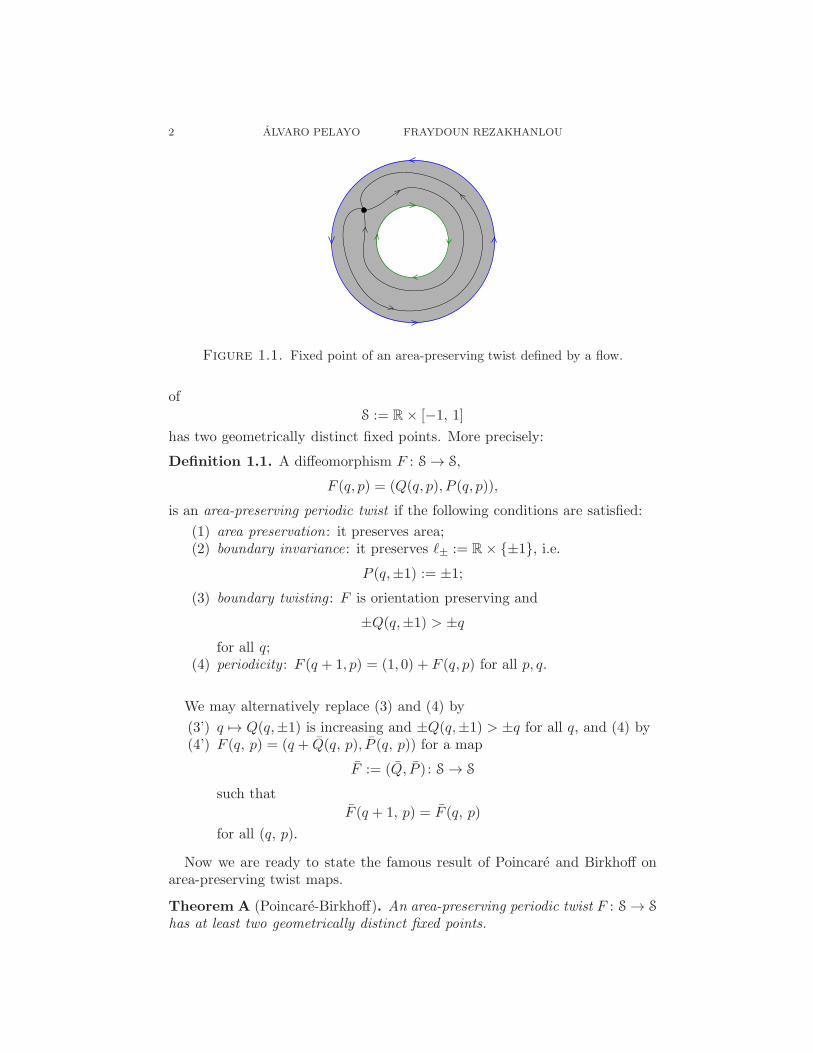
Figure 1.1. Fixed point of an area-preserving twist defined by a flow.
of
S := R× [−1, 1]
has two geometrically distinct fixed points. More precisely:
Definition 1.1. A diffeomorphism F : S → S,
F (q, p) = (Q(q, p), P (q, p)),
is an area-preserving periodic twist if the following conditions are satisfied:
(1) area preservation: it preserves area;(2) boundary invariance: it preserves ℓ± := R× ±1, i.e.
P (q,±1) := ±1;
(3) boundary twisting : F is orientation preserving and
±Q(q,±1) > ±q
for all q;(4) periodicity : F (q + 1, p) = (1, 0) + F (q, p) for all p, q.
We may alternatively replace (3) and (4) by
(3’) q 7→ Q(q,±1) is increasing and ±Q(q,±1) > ±q for all q, and (4) by(4’) F (q, p) = (q + Q(q, p), P (q, p)) for a map
F := (Q, P ) : S → S
such that
F (q + 1, p) = F (q, p)
for all (q, p).
Now we are ready to state the famous result of Poincare and Birkhoff onarea-preserving twist maps.
Theorem A (Poincare-Birkhoff). An area-preserving periodic twist F : S → S
has at least two geometrically distinct fixed points.
POINCARE-BIRKHOFF THEOREMS IN RANDOM DYNAMICS 3
For the purpose of our article, the most useful proof of Theorem A fol-lows Chaperon’s viewpoint [Ch84, Ch84b, Ch89] and the so called theory of“generating functions”. Generalizations including a number of new ideas havebeen obtained by several authors, eg. see Carter [Ca82], Ding [Di83], Franks[Fr88, Fr88b, Fr06], Le Calvez-Wang [Le10], Neumann [Ne77], and Jacobowitz[Ja76, Ja77]. Theorem A was proved1 in certain cases by Poincare [Po12].Later Birkhoff gave a full proof and presented generalizations [Bi13, Bi26]; in[Bi66] he explored its applications to dynamics. See [BG97, Section 7.4] and[BN77] for an expository account.
There is no unique way to generalize Theorem A, but at least one shouldhope that a generalization to the random setting recovers it as a particu-lar case. In our paper we prove a parallel generalization of Theorem A totwist maps that are random with respect to a given probability measure. Ourstochastic model in the so called periodic case coincides with the classicalsetting of Poincare-Birkhoff theorem. While random dynamics has been ex-plored quite throughly, eg. Brownian motions [Ei56, Ne67], the implicationsof the area preservation assumption remain relatively unknown. We recom-mend [AA68, KH95, Ko57, Mo73, Sm67] for modern accounts of dynamics,and [BH12, HZ94, MS98, Pol01] for treatments emphasizing symplectic tech-niques.
2. The space of all twist maps and Main Theorems
The primary goal of this article is the study of the set of fixed points ofan area preserving twist map that is not necessarily periodic. To describeour results, let us write T for the space of area preserving twist maps. Thatis, the set of diffeomorphism F : S → S, such that the Axioms (1) − (3) ofIntroduction are valid. For our purposes, let us also write T for the space ofmaps F : S → S such that if
ℓ(F )(q, p) := (q, 0) + F (q, p),
then ℓ(F ) ∈ T. We think of the operator ℓ : T → T as sending F to its liftF = ℓ(F ). We have a natural family of shifts
τa : T → T : a ∈ R
, that aredefined by
τaF (q, p) = F (q + a, p).
Given F ∈ T, we write
Fix(F ) =
x ∈ S : F (x) = x
⊂ S,
for the set of its fixed points. If we abuse the notation and write τa for
τaA = x : x+ a ∈ A,
then we have the trivial commutative relationship
(2.1) τaFix(ℓ(F )) = Fix(ℓ(τaF )).
1One can use symplectic dynamics to study area-preserving maps, see [BH12]. Section3.4 of Bramham et al. [BH12] proves Theorem A using the important tool of finite energyfoliations [HWZ03].
4 ALVARO PELAYO FRAYDOUN REZAKHANLOU
The type of results we will establish in this paper have the following fla-vor: For generic members of T we will show that the set Fix(F ) is infinite,and in some cases of positive density. We use probabilist means to decide ongenericness; we explore quantitative properties of Fix(F ) that are valid withprobability one with respect to a probability measure that is defined on theset T, or equivalently on T. More precisely, we take a probability measure Q
on (T,F), where F denotes the Borel σ-algebra associated with the topologyof uniform norm, and show that the probability of those F for which the setFix(ℓ(F )) enjoys certain quantitative properties is one. The type of quanti-tative properties we have in mind, would not be affected if the set Fix(F ) istranslated. In view of the translation property (2.4), it is natural to assumethat the probability measure Q is translation invariant (or in the probabilitytheory jargon stationary). This property also allows us to apply the ErgodicTheorem to guarantee that density of Fix(ℓ(F )) is well-defined for Q-almostall choices of F . We also assume that the probability measure Q is ergodicwith respect to the translations τa : a ∈ R. This is simply an irreducibilityassumption; if Q is not ergodic, then we can express it as an average over itsergodic components and our results would be valid for each component. Theadvantage/raison d’etre of the ergodicity is that the Q-almost sure density ofFix(F ) is a constant independent of F .
We note that in the periodic case, the fact that we have at least two ge-ometrically distinct fixed points, translates to asserting that in the interval[0, ℓ], ℓ ∈ N, there are at least 2ℓ fixed points. How much of this is true in therandom case? On account of Theorem A, let us formulate a wish-list that wewould like to have for the set of fixed points Fix(F ) of a randomly selectedarea-preserving twist map F (·, ·):
(i) At the very least, we would like to show that the set Fix(F ) is nonempty(and in fact unbounded from both sides by ergodicity) almost surely.
(ii) Better yet, we would like to show that the set Fix(F ) has a positive density.That is, the large ℓ limit of ℓ−1#
(
Fix(F )∩ [0, ℓ])
exists and is positive almostsurely. (For a set B, #B denote its cardinality.)
(iii) Ideally, we can come up with two distinct properties (formulated in termsof the derivative dF at the fixed point) such that if the set of fixed points withthose properties are denoted by Fix1(F ) and Fix2(F ), then both Fix1(F ) andFix2(F ) are of positive density almost surely. This would be our analog of “twogeometrically distinct” aspect of Poincare-Birkhoff Theorem in the randomsetting.
2.1. Monotone Twist Maps. As we will demonstrate in our first theorem,we have a rather satisfactory result in the case that Q is concentrated on thespace of monotone twists.
Definition 2.1. (1) We write MT+ for the space of maps F = (Q, P ) ∈ T
such that for every q, the function f : [−1, 1] → R, given by f(p) := Q(q, p) isincreasing. We also write MT+ for the set of ℓ(F ), with F ∈ MT+. We refer
POINCARE-BIRKHOFF THEOREMS IN RANDOM DYNAMICS 5
to the members of MT+ as the (positive) monotone twist maps. Similarly, wewrite MT− for the space of maps F such that F−1 ∈ MT+. We refer to themembers of MT− as the negative monotone twist maps.
(2) A fixed point x = (q, p) of F (·, ·) : S → S is of + (respectively -) type ifthe eigenvalues of dF (q, p) are positive (respectively negative). We write
Fix±(F ) =
x ∈ Fix(F ) : x is of ± type
.
Our interest in MT± stems from the fact that all monotone twist mapspossess generating functions. That is, for F = ℓ(F ) ∈ MT+, we can find ascalar-valued function G(q,Q) = G(q,Q; F ) such that
(2.2) F (q,−Gq(q,Q)) = (Q,GQ(q,Q)).
Because of the boundary conditions of F (q, p) = (P (q, p), Q(q, p)), we onlyneed to define G(q,Q) for the pair (q,Q), such that
(2.3) Q(q,−1) 6 Q 6 Q(q,+1).
In particularψ(q; F ) := G(q, q; F ),
is well defined. As we will see later (see (2.4) below)
ψ(·; τaF ) = τaψ(·; F ).
This implies that the law of ψ(q; F ) is translation invariant (hence independentof q), by the stationarity of Q.
As is demonstrated in our Theorem B below, (iii) of our wish-list is (almost)materialized for randomly selected monotone twist maps:
Theorem B. Let Q be a translation invariant ergodic probability measure on(
T,F)
, such that Q(
MT+
)
= 1. Then the following statements are true withprobability one with respect to Q:
(1) The sets Fix±(
ℓ(F ))
are nonempty.
(2) If the random pair(
d
dqψ(q; F ),
d2
dq2ψ(q; F )
)
,
has a probability density ρ(a, b) (which is independent of q by translation in-variance), then the sets Fix±
(
ℓ(F ))
have positive density λ±, given by
λ± =
∫ ∞
−∞
b±ρ(0, b) db.
As we mentioned earlier, each monotone twist map has a generating func-tion that is unique modulo a constant. It may appear that it would be hardto come up with examples of probability measures that are concentrated onmonotone twist maps because the set MT+ is rather complicated; after all afunction F ∈ MT+ must satisfy (1) − (3) of the Introduction, and the mono-tonicity condition. However, it would be easier if we start from a randomly
6 ALVARO PELAYO FRAYDOUN REZAKHANLOU
selected generating function G, and construct F from it with the aid of (2.2).For this to be useful, we need to figure out what conditions must be satisfiedby G in order to be in the range of the map F 7→ G(·, ·; F ). It is not hard tosee
(2.4) G(q + a,Q+ a; F ) = G(q,Q; τaF ).
(See Section 5.) This suggests defining L by
G(q,Q; F ) = L(q,Q− q; F ),
and try to find the range of the map A(F ) := L(·, ·; F ). In some sense,L(q, v) = L(q, v; F ) is the Lagrangian of F , with v playing the role of thevelocity. We also note that in terms of the Lagrangian,
ψ(q; F ) = L(q, 0; F ).
For our second result, we determine the range of the map A and give a preciserecipe for constructing A−1, and an ergodic stationary law on MT+. We notethat in view of (2.3), the domain of definition for the function L(q, v) is
Q(q,−1) 6 v 6 Q(q, 1).
However, it is more convenient to start with an extension of L to R2, andfigure out what the domain of L is from this extension. To have a simplerdescription for the operator A−1, we would even start from a suitable translateof the extended Lagrangian function, denoted by ω, and build G from thistranslation. In the following Definition, we give the necessary axioms for ωand make preparations for the construction of G from ω.
Definition 2.2. Let us write Ω0 for the space of functions
ω : R2 → R
such that ω(q, a) > 0 for a > 0, ω(q, 0) = 0, and,
η(q;ω) = infa | ω(q, a) = 2 <∞,
for every q. We then set
Q−(q;ω) =1
2
∫ η(q;ω)
0ω(q, a)da− η(q;ω),
G(q,Q;ω) = ω(q,Q− q −Q−(q;ω)).
We write Ω1 for the space of ω ∈ Ω0 such that Gq(q,Q;ω) < 0 for all (q,Q).
Theorem C. For every ω ∈ Ω1, there exists a unique function F (·, ·;ω) suchthat if F (·, ·;ω) = ℓ
(
F (·, ·;ω))
, then the equation (2.2) is valid for the functionG(q,Q) = G(q,Q;ω), that is given by
G(q,Q;ω) =
∫ Q
q+Q−(q;ω)ω(q, a)da− (Q− q).
Moreover, if τaω(q, v) = ω(q + a, v), then
(2.5) F (·, ·; τaω) = τaF (·, ·;ω).
POINCARE-BIRKHOFF THEOREMS IN RANDOM DYNAMICS 7
Theorem C provides a recipe for constructing examples of randommonotonetwist maps for which Theorem B is applicable.
Recipe for Monotone Twist Map: Take any probability measure P on Ω0
that is stationary and ergodic with respect to τa : a ∈ R. If P(Ω1) = 1,then the push forward Q := B♯P of P with respect to the map
B : Ω1 → MT+, B(ω)(·, ·) = F (·, ·;ω),
gives a stationary and ergodic probability measure on MT+.It is straightforward to construct stationary and ergodic probability mea-
sures on Ω0. The only nontrivial condition to worry about is P(Ω1) = 1. Tosee how in practice such a condition is verified, let us consider a concreteexample.
Example 2.3 If we assume that ω is linear in a, and write ω(q, a) = R(q)a,for a function R : R → R, then ω ∈ Ω0 means that R > 0. On the other hand,if the derivative of R satisfies 2|R′| 6 R2, P-almost surely, then P(Ω1) = 1. Forexample, we can start from an arbitrary uniformly positive stationary processR0 with bounded derivative, and build ω via ω(q, a) = cR0(q)a. This wouldsatisfy P(Ω1) = 1 provided that c is sufficiently large. See Example 5.7 fordetails.
2.2. Hamiltonian Systems. We now describe an important class of twistmaps that may include non-monotone examples. Let Ω2 denote the set C2
(Hamiltonian) functions ω(q, p, t) with uniformly bounded second derivativessuch that
±ωp(q,±1, t) > 0, ωq(q,±1, t) = 0.
(Note that even though ω(q,±1, t) is independent of q, the function ωp(q,±1, t)may depend on q.) Given ω ∈ Ω2, set
τaω(q, p, t) = ω(q + a, p, t),
as before, and write φωt (q, p) for the flow of the corresponding Hamiltoniansystem
q = ωp(q, p, t), p = −ωq(q, p, t).
It is not hard to show that if
F t(q, p;ω) = φωt (q, p), F t(q, p;ω) = φωt (q, p)− (q, 0),
then F t(·, ·;ω) ∈ T, and
F t(
q, p; τaω)
= τaFt(
q, p;ω)
.
This means that if we start with a τ -invariant ergodic probability measure P
on Ω2, then its push-forward Qt under the map ω 7→ F t(·, ·;ω) is a τ -invariantergodic probability measure on MT+.
8 ALVARO PELAYO FRAYDOUN REZAKHANLOU
Theorem D. Let P be a τ -invariant ergodic probability measure P on Ω2.Then the probability that F t(·, ·;ω) has infinitely many fixed points is one forevery t ≥ 0, i.e.
P(
#Fix(
F t(·, ·, ;ω))
= ∞)
= 1.
Example 2.4 In contrast with Theorem C, it is not hard to come up with ex-amples of Qt because any q-stationary process ω(q, p, t) does the job providedthat the boundary conditions are satisfied. Here are two examples:
(i) Let A(q, t) be a positive C2, q-stationary random process with boundedsecond q-derivative. Take any deterministic C2 function B(p, t) with boundedsecond p-derivative such that ±Bp(±1, t) > 0, and B(±1, t) = 0. Then theHamiltonian function ω(q, p, t) = A(q, t)B(p, t) will be in Ω2.
(ii) One classical way of constructing a stationary Hamiltonian function isstarting from a fixed deterministic Hamiltonian functionH0(q, p, t) of compactsupport in q-variable that satisfies the boundary conditions, and set
ω(q, p, t;α) =∑
i
H0(q − qi, p, t),
where
α = qi : i ∈ Z,
is a stationary point process. By this we mean that the set α is a discretesubset R that is selected randomly with a law that is invariant with respectto the translations
τaα = q − a : q ∈ α.
A Poisson point process of constant intensity is an example of a stationarypoint process.
Theorem C raises two questions:
(i) Let Q be a stationary ergodic measure on T. Can we find a stationaryergodic measure P on Ω2 such that Q = Q1? In other words, Q is thepush-forward of P with respect to the map ω 7→ F 1(·, ·;ω)?
(ii) What can be said about the type of the fixed points we have in The-orem D?
To rephrase the first question, let us write C([0, 1];T) for the space of C1
maps γ : [0, 1] → T, such that ℓ(γ(0)) is identity. The shift operator τ onT induces a shift operator (again denoted by τ) on C([0, 1];T) by (τaγ)(t) =τa(γ(t)). Note that if we have a stationary ergodic measure P on Ω2, then themap
ω 7→(
F t(q, p;ω) = φωt (q, p)− (q, 0) : t ∈ [0, 1])
,
pushes forward P onto a stationary ergodic probability measure Q on C([0, 1];T).It is not hard to show that the converse is also true; a stationary ergodic proba-bility measure Q on C([0, 1];T) is necessarily comes from a unique a stationaryergodic measure P on Ω2. As a result, we may rephrase the first question as
POINCARE-BIRKHOFF THEOREMS IN RANDOM DYNAMICS 9
(i’) Let Q be a stationary ergodic measure on T. Can we find a stationaryergodic measure Q on C([0, 1];T), such that Q is the push forward of Qunder the time-1 map π1 : C([0, 1];T) → T? (By time-1 map we meanπ1γ := γ(1).)
We conjecture that the answer to this question is affirmative. In Theorem Ebelow, we partially resolve this conjecture by showing that if there is a pathγ such that ℓ(γ) is area preserving only in the average sense, then it can bedeformed to a path of area preserving maps. To state this carefully, we makea definition.
Definition 2.5. Let D denotes the space of diffeomorphism F : S → S.We write D for the space of functions F such that ℓ(F ) ∈ D. Let Q be astationary ergodic measure on C([0, 1];D). We say that Q is regular if thefollowing conditions are true:
(a)∫
supt∈[0,1]
[
‖γ(t)‖∞ + ‖dγ(t)‖∞ +∥
∥dγ(t)−1∥
∥
∞
]
Q(dγ) <∞,
with ‖ · ‖∞ denoting the L∞ norm, and γ(t) and dγ(t) denoting thederivatives of γ(t) with respect to t and x = (q, p).
(b)
1
2
∫[∫ 1
−1det(dγ(t)(q, p)) dp
]
Q(dγ) = 1;
for every t ∈ [0, 1]. (This expression is independent of q by the sta-tionarity of Q.)
We note that the condition (b) is trivially satisfied if Q is concentrated onC([0, 1];T), because for an area preserving ℓ(γ(t)), we simply have
det(dγ(t)(q, p)) = 1.
Theorem E. Let Q be a stationary ergodic measure on T. If there exists aregular stationary ergodic measure Q on C([0, 1];D), such that Q is the pushforward of Q under the time-1 map π1γ := γ(1), then there exits anotherstationary ergodic measure Q′ on C([0, 1];T), such that Q is also the pushforward of Q under the time-1 map π1.
2.3. The Complexity of an Isotopy. We now would like to address thesecond question we asked in Subsection 2.2:
(ii) What can be said about the type of the fixed points we have in The-orem D?
To address this question, we first need to explain what role the measure Q
on C([0, 1];T) plays in the proof of Theorem D. When the measure Q on T
comes from a measure P on Ω2, or when the assumptions of Theorem D aresatisfied, we have an isotopy of area preserving twists F t(·, ·;ω) that connectsthe identity to F (·, ·;ω) := F 1(·, ·;ω), with F 1 distributed according to Q.
10 ALVARO PELAYO FRAYDOUN REZAKHANLOU
Following the Chaperon’s strategy for proving Conley-Zehnder’s Theorem, wemay use this isotopy to express F as a finite composition of monotone twistmaps. More precisely,
Theorem F. Let P be a τ -invariant ergodic probability measure P on Ω2. LetF = F 1 be as in Theorem D. Then there exists a deterministic integer N > 0and area-preserving random twists Fj , 0 6 j 6 N, such that for P almost allω ∈ Ω2, we have a decomposition:
(2.6) F (·, ·;ω) = FN (·, ·;ω) . . . F2(·, ·;ω) F1(·, ·;ω) F0(·, ·;ω),
where
• Fj is negative monotone if j is even;• Fj is positive monotone if j is odd;• Fj(q, p;ω) := Fj(q, p;ω) − (q, 0) is stationary i.e. Fj(q, p; τaω) =τaFj(q, p;ω), for every j.
The integer N in (2.6) is the complexity of F . We may use an L∞ boundon the first derivative of ω to get an upper bound on N . Statements [Le91,Propositions 2.6 & 2.7, Lemma 2.16] have the flavor to Theorem F for classicaltwists (see also [MS98, Section 9.2]).
When N = 1 or 2, more can be said about the set of fixed points and thenature of dF at the fixed points. We refer to Theorems 6.5 and 6.6 whenN = 1, and Theorem 7.3 when N = 2.
2.4. Almost periodic twists. In fact our main results do cover the clas-sical Poicare-Birkhoff Theorem A in some cases. For example, Theorem Dimplies that the flow of any deterministic Hamiltonian function H0(q, p, t) onstrip S, that is 1-periodic in q, and satisfies the twist boundary conditions(H0
q (q,±1, t) = 0,±H0p (q,±, t) > 0), possesses 1-periodic orbits (or its time
one map has fixed points). In other words, we may recast the deterministicperiodic model as an example of a random twist model. The interpretationwe have in mind is also applicable if H0 is almost periodic in q. We explainthis by three models of random area-preserving twist maps:
Example 2.6 (Periodic Twists) As the simplest example, take any F0 ∈ T,that is 1-periodic in q-variable, and set
(2.7) Γ(F0) =
τaF0 : a ∈ R
⊂ T.
We now take a τ -invariant probability measure Q on T that is concentratedon Γ(F0). Since F0 is a 1-periodic function in q-variable, the set Γ(F ) ishomeomorphic to the circle. (Here were are thinking of circle as the interval[0, 1] with 0 = 1.) Since Q is τ -invariant, it can only be the push forward of theLebesgue measure under the map a 7→ τaF . Now any almost sure statementfor the fixed points of the lifts of maps in the support of Q is equivalent toan analogous statement for the map F0. This is because if (q0, p0) is a fixedpoint for
F (q, p) := ℓ(
τaF)
= (q, 0) + τaF0(q, p),
POINCARE-BIRKHOFF THEOREMS IN RANDOM DYNAMICS 11
then (q0 + a, p0) is a fixed point for F0 = ℓ(F0). For example, the statementthat for Q-almost choices of F , its lift ℓ(F ) has a fixed point is equivalentto asserting that F0 has a fixed point. In summary, our stochastic modelcoincides with the classical setting of Poincare-Birkhoff in this case.
Example 2.7 (Quasi-periodic twists) Pick a function
F1 : Tk × [−1,−1] → R× [−1, 1],
where Tk denotes the k-dimensional torus. Pick a vector v ∈ Rk that satisfiesthe following condition:
(2.8) 〈v, n〉 = 0, n ∈ Zk ⇒ n = 0.
Let
F0(q, p) = F1(qv, p)
and define Γ(F0) as in (2.7). Note that if k > 1, the set Γ(F0) is not closed.However, the condition (2.8) guarantees that its topological closure Γ′(F0)consists of functions of the form
F (q, p; b) = F0(qv + b, p),
with b ∈ Tk. (Here we regard Tk as [0, 1]k with 0 = 1, and qv − b is a Mod1 summation.) Assume that Q is concentrated on the set Γ′(F0). Again,since Q is τ -invariant, the pull-back of Q with respect to the transformationb ∈ Tk 7→ F (·, ·; b) can only be the uniform measure on Tk. Hence, a Q-almostsure statement regarding the fixed points of F = ℓ(F ), is equivalent to ananalogous statement for the map
F (·, ·; b) = ℓ(
F (·, ·; b))
,
for almost all b ∈ Tk. In other words, our main result does not guarantee theexistence of fixed points for a given quasi-periodic map F0 = ℓ(F0). Insteadour main results say that for almost all choices of b, the map F (·, ·; b) possessesfixed points.
Example 2.8 (Almost periodic-twists) Given a function F0 ∈ T, let us assumethat the corresponding Γ(F0) is precompact with respect to the topology ofuniform convergence. We write Γ′(F0) for the topological closure of Γ(F0). Bythe classical theory of almost periodic functions, the set Γ′(F0) can be turnedto a compact topological group and for Q, we may choose a normalized Haarmeasure on Γ′(F0). Again, our main results only guarantee the existence offixed points for F (q, p) = ℓ(F ), for Q-almost all choices of F .
In the random stationary setting, we may start with a function F0 such thatthe corresponding Γ′(F0) is not compact and may not have a group structure.Instead we may insist on the existence of an ergodic translation invariantmeasure that is concentrated on Γ′(F0). Even the last requirement can berelaxed and our measure Q may not be concentrated on Γ′(F0) for some F0.The measure Q in some sense plays the role of the normalized Haar measurein our third example above.
12 ALVARO PELAYO FRAYDOUN REZAKHANLOU
2.5. Abstract Formulation. So far we have stated several results for theset of fixed point of ℓ(F ) where F is selected according to a suitable ergodicstationary probability measure Q on T. In all the models we have discussedin the preceding subsections, the measure Q is expressed as a push forwardof another ergodic stationary probability measure P that is now defined on aprobability space Ω. In other words, our Q-selected function can be expressedas F (·, ·;ω) with ω selected according to a suitable stationary ergodic measureP, and the map ω 7→ F (·, ·;ω) satisfies
τaF (·, ·;ω) = F (·, ·; τaω).
This is equivalent to
(2.9) F (q, p;ω) = F (0, p; τqω) := F0(τqω, p).
The space Ω takes different forms depending on the type of result we have inmind. For example
• Ω = Ω1 where Ω1 is the space of functions in Ω0 that satisfies a suitablenondegeneracy condition as was discussed in Subsection 2.1.
• Ω = Ω2 is the space of certain Hamiltonian functions as we describedin Subsection 2.3.
• Ω = Γ′(F0) is the topological closure of the translates of a fixed F0 ∈ T
as we discussed in Subsection 2.4.
For a more flexible formulation, we set up a framework for random area-preserving twist map that is defined on a general and unspecified Ω. Withthis goal in mind, we propose the following abstract setting to study area-preserving dynamics: a probability space, that is, a quadruple:
Ω := (Ω, F, P, τ).(2.10)
Here Ω is a separable metric space, F is the Borel sigma-algebra on Ω, τ : R×Ω → Ω is a continuous R-action, and P is a τ -invariant ergodic probabilitymeasure on (Ω,F). Denote τa := τ(a, ·) : Ω → Ω. In addition, we assume:
(i) P-positivity : if U ∈ F is a nonempty open set, then P(U) > 0.(ii) P-preservation by τ : P(τaA) = P(A) for every a ∈ R, and every A ∈ F.(iii) Ergodicity : for every A ∈ F, if τaA = A for all a ∈ R, then P(A) = 1 or
P(A) = 0.
If (i), (ii), and (iii) hold we say that P is a τ -invariant ergodic probabilitymeasure. For instance, take a smooth manifold Ω which admits a smoothglobal flow φ : R × Ω → Ω with an ergodic invariant probability measure P
that is positive on nonempty open subsets of Ω (it is non-trivial to find φ withthese properties), F the Borel sigma-algebra of Ω, and τa := φ(a, ·).
In what follows, let Ω be a probability space as in (2.10). Let
F0 : Ω× [−1, 1] → S
be a measurable map with respect to the product measure of P and theLebesgue measure on [−1, 1]. Write
F0(ω, p) = (Q(ω, p), P (ω, p))
POINCARE-BIRKHOFF THEOREMS IN RANDOM DYNAMICS 13
and suppose that F : S×Ω → S is of the form F (q, p;ω) = (Q(q, p; ω), P (q, p; ω)),with
(2.11)
Q(q, p; ω) = q + Q(τqω, p)
P (q, p; ω) = P (τqω, p).
Write E for the expected value with respect to the probability measure P.
Definition 2.9. We say that F in (2.11) is an area-preserving random twistif the following hold for P-almost all ω:
(1) area-preservation: F (· , · ; ω) : S → S is an area-preserving diffeomor-phism;
(2) boundary invariance: P (q,±1;ω) = ±1;(3) boundary twisting : q 7→ Q(q,±1;ω) is increasing, and ±Q(ω,±1) > 0.
If additionally Q(ω, p) is increasing in p, we refer to F as a (positive) monotonearea-preserving random twist. We call F a negative monotone area-preservingrandom twist, if F−1 is a positive area-preserving random twist. When thereis no danger of confusion, we may simply call such map as a positive/negativetwist.
It is this abstract formulation that will be used for the rest of the paper. Bya slight change of notion, we can readily restate our main results TheoremsB-F in terms of an abstract area-preserving random twist.
2.6. Arnol’d Conjecture. Arnol’d formulated the higher dimensional ana-logue of Theorem A: the Arnol’d Conjecture [Ar78] (see also [Au13], [Ho12],[HZ94], [Ze86]). The first breakthrough on the conjecture was by Conley andZehnder [CZ83], who proved it for the 2n-torus (a proof using generatingfunctions was later given by Chaperon [Ch84]). The second breakthroughwas by Floer [Fl88, Fl89, Fl89b, Fl91]. Related results were proven eg. byHofer-Salamon, Liu-Tian, Ono, Weinstein [Ho85, HS95, LT98, On95, We83].
The first breakthrough on Arnold’s Conjecture was achieved by Conleyand Zehnder [CZ83]. According to their theorem, any smooth symplecticmap F : T2d → T2d that is isotopic to identity has at least 2d + 1 manyfixed points. For the stochastic analog of [CZ83], we take a 2d-dimensionalstationary process
X(x;ω) = X(τxω)
withX : Ω → R2d; x ∈ R2d,
and assume that its lift
F (x;ω) = x+X(x;ω)
is symplectic with probability one. Our strategy of proof is also applicableto such random symplectic maps. The main ingredients for proving resultsanalogous to our main theorems are Morse Theory and Spectral Theoremfor multi-dimensional stationary processes. In a subsequent paper, we willwork out a generalization of Conley and Zehnder’s Theorem in the stochasticsetting.
14 ALVARO PELAYO FRAYDOUN REZAKHANLOU
2.7. Main Strategy and Outline of the Paper. As we mentioned earlier,we have adopted Chaperon’s approach to establish our main results. Here isan outline of what follows:
(i) In Section 3 we give a definition for the generalized generating function ofan area-preserving twist map F in our random setting and show that there isa one-to-one corresponding between fixed points F and the critical points ofits generalized generating function (Proposition 3.3).
(ii) The purpose of Section 4 is threefold:
• We show that if (2.6) is valid for F , then F has a generalized generatingfunction. On account of Proposition 3.3, we may prove our resultsabout the fixed points of F by proving analogous results for the criticalpoints of its generalized generating function. (See Lemma 4.4.)
• We establish Theorem F so that (2.6) is valid whenever our area-preserving random twist map comes from a Hamiltonian ODE.
• We establish Theorem E so that any regular Q comes from a Hamil-tonian ODE.
(iii) By Theorem F, we can associate a nonnegative integer N to our twist mapthat measures its complexity. The case N = 0 corresponds to the monotonetwist maps and they are studied in Section 5. In particular, we establishTheorems B and C in this Section.
(iv) In Sections 6 and 7 we study the case of an area-preserving twist map withcomplexity N ≤ 2. Most notably we show that if N = 1, then the correspond-ing F possesses infinitely many fixed points of different types (Theorems 6.5,6.6). In the case of N = 2, we have a similar result for the critical points ofits generating function. Though we have not been able to prove an analogousresult for the fixed points of F because of a complicated formula that relatesthe eigenvalues of the first derivative of F to the the second derivatives of itsgenerating function.
(v) Section 8 is devoted to the proof of Theorem D.
3. Calculus of random generating functions
We construct the principal novelty of the paper, random generating func-tions, and explain how to use them to find fixed points. Recall that Ω is as in(2.10).
Definition 3.1. We say that a measurable function G : Ω → R is ω-differentiable if the limit
∇G(ω) := limt↓0
t−1 (G(τtω)−G(ω))
exists for P-almost all ω. For a measurable map K : Ω× [0, 1] → R we writeKp =
∂K∂p
and Kω = ∂K∂ω
for the partial derivatives of K. We say that K is C1
if the partial derivatives of K exist and are continuous for P-almost all ω.
POINCARE-BIRKHOFF THEOREMS IN RANDOM DYNAMICS 15
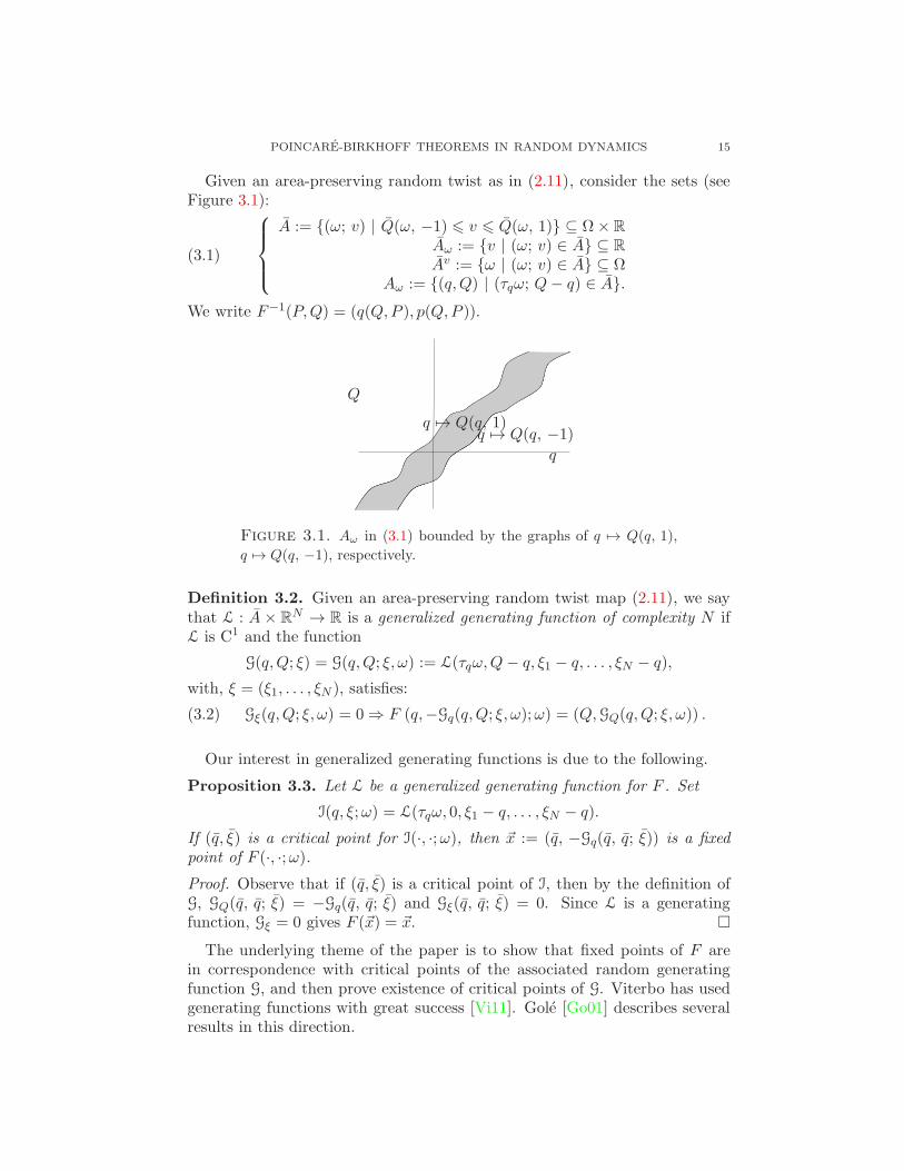
Given an area-preserving random twist as in (2.11), consider the sets (seeFigure 3.1):
A := (ω; v) | Q(ω, −1) 6 v 6 Q(ω, 1) ⊆ Ω× R
Aω := v | (ω; v) ∈ A ⊆ R
Av := ω | (ω; v) ∈ A ⊆ ΩAω := (q,Q) | (τqω; Q− q) ∈ A.
(3.1)
We write F−1(P,Q) = (q(Q,P ), p(Q,P )).
Q
q 7→ Q(q, −1)
q
q 7→ Q(q, 1)
Figure 3.1. Aω in (3.1) bounded by the graphs of q 7→ Q(q, 1),
q 7→ Q(q, −1), respectively.
Definition 3.2. Given an area-preserving random twist map (2.11), we saythat L : A× RN → R is a generalized generating function of complexity N ifL is C1 and the function
G(q,Q; ξ) = G(q,Q; ξ, ω) := L(τqω,Q− q, ξ1 − q, . . . , ξN − q),
with, ξ = (ξ1, . . . , ξN ), satisfies:
(3.2) Gξ(q,Q; ξ, ω) = 0 ⇒ F (q,−Gq(q,Q; ξ, ω);ω) = (Q,GQ(q,Q; ξ, ω)) .
Our interest in generalized generating functions is due to the following.
Proposition 3.3. Let L be a generalized generating function for F . Set
I(q, ξ;ω) = L(τqω, 0, ξ1 − q, . . . , ξN − q).
If (q, ξ) is a critical point for I(·, ·;ω), then ~x := (q, −Gq(q, q; ξ)) is a fixedpoint of F (·, ·;ω).
Proof. Observe that if (q, ξ) is a critical point of I, then by the definition ofG, GQ(q, q; ξ) = −Gq(q, q; ξ) and Gξ(q, q; ξ) = 0. Since L is a generatingfunction, Gξ = 0 gives F (~x) = ~x.
The underlying theme of the paper is to show that fixed points of F arein correspondence with critical points of the associated random generatingfunction G, and then prove existence of critical points of G. Viterbo has usedgenerating functions with great success [Vi11]. Gole [Go01] describes severalresults in this direction.
16 ALVARO PELAYO FRAYDOUN REZAKHANLOU
4. Proofs of Theorems E and F
We begin by introducing stationary lifts.
Definition 4.1. A function f(q, ω) is stationary if f(q, ω) = f(τqω) for acontinuous f : Ω → R. We say that f is a stationary lift if f(q, ω) = q+ f(τqω)for a continuous f : Ω → R.
Definition 4.2. A vector-valued map f(q, p;ω) with f(·, ω) : R2 → R2 isq-stationary if f(q, p, ω) = f(τqω, p) for some f : Ω × R → R2. A similardefinition is given for f(·, ω) : S → R2. We say that such f is a q-stationarylift if f can be expressed as f(q, p, ω) = (q, 0) + f(τqω, p).
Proposition 4.3. The following properties hold:
(P.1) If f(q, ω) is an increasing stationary lift in C1, then f−1 is an increasinglift. The same holds for q-stationary diffeomorphism lifts f(q, p, ω).
(P.2) The composition of q-stationary lifts is a q-stationary lift. If f is aq-stationary lift and g is q-stationary, g f is q-stationary.
(P.3) For every differentiable f : Ω → R we have that E∇f = 0.
Proof. The proof of (P.2) is trivial. We only prove (P.1) for a stationarylift f(q, p, ω) because the case of f(q, ω) is done in the same way. Assumethat f(q, p, ω) is a q-stationary lift so that for every a ∈ R, f(q + a, p, ω) =(a, 0)+f(q, p, τaω), and write g(q, p, ω) for its inverse. To show that g(q, p, ω) isa q-stationary lift it suffices to check that g(q + a, p, ω) = (a, 0) + g(q, p, τaω).In order to do this, let us fix a and write g(q, p, ω) for the right-hand side(a, 0) + g(q, p, τaω). Observe that since f is a q-stationary lift,
f(g(q, p, ω), ω) = (a, 0) + f(g(q, p, τaω), τaω) = (a, 0) + (q, p) = (q + a, p).
By uniqueness, g(q, p, ω) = g(q + a, p, ω), which concludes the proof of (P.2).As for (P.3), write f(x, ω) = f(τxω) and observe that for any smooth J : R →R of compact support, with
∫
R J(x)dx = 1,
E∇f =
∫
R
J(x) (Efx(x, ω)) dx
= −E
∫
R
J ′(x)f(x, ω) dx
= −
(∫
R
J ′(x) dx
)
(
Ef)
,(4.1)
so E∇f = 0.
The proof of Theorem E draws on spectral theory for random processes.To this end, let us recall the statement of the Spectral Theorem for randomprocesses. The Spectral Theorem allows us to represent a random process interms of an auxiliary process with randomly orthogonal increments. Such arepresentation reduces to a Fourier series expansion if the stationary processis periodic. In order to apply the Spectral Theorem to a stationary processa(q) = a(τqω), one follows the steps:
POINCARE-BIRKHOFF THEOREMS IN RANDOM DYNAMICS 17
(i) Assume that a(q) is centered in the sense that Ea(ω) = 0. We definethe correlation R(z) = Ea(ω)a(τzω).
(ii) There always exists a nonnegative measure G such that
R(z) =
∫ ∞
−∞
eizξG(dξ).
(iii) One can construct an auxiliary process (Y (ξ) : ξ ∈ R) or alternativelythe random measure Y (dξ) = Y (dξ, ω) that are related by Y (I) =Y (b)−Y (a), where I = [a, b]. The process Y has orthogonal incrementsin the following sense:
I ∩ J = ∅ =⇒ EY (I)Y (J) = 0.(4.2)
The relationship between the measure G(dξ) or its associated nonde-creasing function G(ξ) is given by EY (I)2 = G(b) −G(a) = G(I).
The Spectral Theorem ([Do53]) says that for any stationary process a forwhich Ea2 <∞, we may find a process Y satisfying (4.2) such that a(τqω) =∫∞
−∞eiqξY (dξ). Note that
Ea(τqω)a(ω) = E
∫ ∞
−∞
eiqξ Y (dξ)
∫ ∞
−∞
Y (dξ′) =
∫ ∞
−∞
eiqξG(dξ).(4.3)
Also, a(ω) =∫∞
−∞Y (dξ, ω), and the stationarity of a(q, ω) means
Y (dξ, τqω) = eiqξY (dξ, ω).
For our application below, we will have a family of random maps (a(q, t) | t ∈[0, 1]) that varies smoothly with t. In this case we can guarantee that theassociated measures Y (dξ, t) depend smoothly in t.
The main difficulties of the proof are due to the fact that the “random andarea-preservation properties” do not integrate well, for instance when arguingabout t-dependent deformations which must preserve both properties. Theproof consists of four steps.
Proof of Theorem E. Write x = (q, p). Since F is random isotopic to theidentity, there is a path F = (F t | t ∈ [0, 1]) of diffeomorphisms that connectsF to the identity map, F t is a stationary lift for each t ∈ [0, 1], we have the
normalization 12
∫ 1−1 E det(dF t)dp = 1 for every t ∈ [0, 1], and F t is regular for
a constant independent of t. There are four steps to the proof:Step 1. (General strategy to turn F into a path of area-preserving randomtwists). Write
ρt(x) = ρt(q, p) = ρt(τqω, p) = det(dF t(x)),
so that (F t)∗ dx = ρt dx, where dx = dq ∧ dp, and by assumption,
1
2
∫ 1
−1Eρtdp =
1
2
∫ 1
−1Eρtdp = 1, ρ0 = ρ1 = 1.
18 ALVARO PELAYO FRAYDOUN REZAKHANLOU
Since F t is regular uniformly on t, the function ρt is bounded and boundedaway from 0 by a constant that is independent of t. That is, there existsa constant C0 > 0 such that C−1
0 6 ρt(x;ω) 6 C0, almost surely. We nowconstruct, out of F t, an area-preserving path Λt which is a stationary liftfor every t. We achieve this by using Moser’s deformation trick, namely weconstruct a path Gt such that Λt = F t Gt is an area-preserving stationarylift for all t. As it will be clear from the construction of Gt below, G0 and G1
are both the identity and, as a result, Λt is a path of area-preserving mapsthat connects F to identity. We need
(Gt)∗(ρtdx) = dx,
and Gt is constructed as a 1-flow map of a vector field
X(x, θ) = X(x, θ; t).
So we wish to find some vector field X such that Gt = φ1 where φθ, θ ∈ [0, 1],denotes the flow of X. In fact, we also have to make sure that the vector field±X is parallel to the q-axis at p = ±1. This guarantees that the strip S isinvariant under the flow of X.
Let
m(θ, x) := θρt(x) + (1− θ),
so that m(θ, x) dx is connecting the area form dx to ρt dx. We need to find avector field X such that its flow φθ satisfies (φθ)∗dx = m(θ, x) dx. Equivalently,m must satisfies the Liouville’s equation
mθ +∇ · (Xm) = ρt − 1 +∇ · (Xm) = 0.(4.4)
The strategy to solve equation (4.4) for X is as follows. Search for a solution X
such that mX = ∇xu is a gradient. Of course we insist that u is q-stationaryso that X is also q-stationary;
u(q, p, θ) = u(τqω, p, θ),
(mX)(q, p, θ) = (mX)(q, p, θ;ω) = (mX)(τqω, p, θ)
= (uω(τqω, p, θ), up(τqω, p, θ)).
Since t is fixed, we drop t from our notations and write ρt = ρ. The equation(4.4) in terms of u is an elliptic partial differential equation of the form
∆u = 1− ρ =: η,(4.5)
with η(q, p) = η(τqω, p) and∫ 1−1 Eη(ω, p)dp = 0. This concludes Step 1.
Step 2. (Applying Spectral Theorem to solve (4.5)). To apply the SpectralTheorem for each p, set
η(ω, p) = η(ω, p)− k(p)
for k(p) = Eη(ω, p), and write
R(q; p) := Eη(ω, p)η(τqω, p) =
∫ ∞
−∞
eiqz G(dz, p).
POINCARE-BIRKHOFF THEOREMS IN RANDOM DYNAMICS 19
Note that Eη(ω, p) = 0 for every p and∫ 1−1 k(p)dp = 0. We have the represen-
tation
η(q, p) = k(p) + η(τqω, p) = k(p) +
∫ ∞
−∞
eiqz Y (dz, p),(4.6)
where Y (dz, p) = Y (dz, p;ω) satisfies
(4.7) Y (dz, p; τqω) = eiqzY (dz, p;ω).
We want to find a solution to the partial differential equation
∆u(q, p) = η(q, p),
which is still stationary in the q variable. First choose h0(p) such that h′′0(p) =k(p) and satisfy the boundary conditions
h0(±1) = 0.(4.8)
We write u = h0 + v and search for a random v satisfying
∆v(q, p) = η(q, p) := η(τqω, p).
Since γ(q, p) = e(iq±p)z is harmonic for each z ∈ R, the function h given by
h(q, p) :=
∫ ∞
−∞
eiqz(
ezp Γ1(dz) + e−zp Γ2(dz))
,(4.9)
is harmonic for any measures Γ1 and Γ2. We will find a solution of the formv = w + h where ∆w = η and h will be selected to satisfy the boundaryconditions vp(q,±1) = 0. Indeed w given by
w(q, p) :=
∫ p
−1
∫ ∞
−∞
eiqz
zsinh((p − a)z)Y (dz, a)da
=
∫ p
−1
∫ ∞
−∞
eiqze(p−a)z − e(a−p)z
2zY (dz, a)da,
satisfies all of the required properties. In order to verify this observe that
wqq(q, p) = −1
2
∫ p
−1
∫ ∞
−∞
zeiqz(
e(p−a)z − e(a−p)z)
Y (dz, a)da,
wp(q, p) =1
2
∫ p
−1
∫ ∞
−∞
eiqz(
e(p−a)z + e(a−p)z)
Y (dz, a)da,
wpp(q, p) =1
2
∫ p
−1
∫ ∞
−∞
zeiqz(
e(p−a)z − e(a−p)z)
Y (dz, a)da + η(q, p).
This clearly implies that ∆w = η.On the other hand, the process w is q-stationary. In other words
w(q, p) = w(q, p;ω) = w(τqω, p),
for a process w. This can be verified by checking that
w(q + b, p;ω) = w(q, p; τbω),
20 ALVARO PELAYO FRAYDOUN REZAKHANLOU
which is an immediate consequence of (4.7):
w(q + b, p;ω) =
∫ ∞
−∞
∫ p
−1
eiqz
zsinh((p− a)z)eibzY (dz, a;ω)da = w(q, p; τbω).
This concludes Step 2.Step 3. (Checking that Γ1 and Γ2 in (4.9) can be chosen to satisfy the boundaryconditions (4.8)). At p = ±1, ±∇u should point in the direction of the q-axis,we need to have that
up(q,±1) = vp(q,±1) = 0,
because h0(±1) = 0. First, the condition vp(q, 1) = 0, means
∫ ∞
−∞
eiqzz(ezΓ1(dz)− e−zΓ2(dz))(4.10)
+1
2
∫ 1
−1
∫ ∞
−∞
eiqz(e(1−a)z + e(a−1)z)Y (dz, a)da = 0,
and the condition vp(q,−1) = 0, means
∫ ∞
−∞
eiqzz(e−zΓ1(dz)− ezΓ2(dz)) = 0.
Since we need to verify the above conditions for all q, we must have thatΓ1 = e2zΓ2, and
zez(e2z − e−2z)Γ2(dz) + Y ′(dz) = 0,
where
Y ′(dz) =1
2
∫ 1
−1(e(1−a)z + e(a−1)z)Y (dz, a)da.
In summary,
(4.11) Γ2(dz) = −z−1e−z(e2z − e−2z)−1Y ′(dz), Γ1 = e2zΓ2.
Since Y satisfies (4.7), the same property holds true for both Γ1 and Γ2. Fromthis it follows that the process h (and hence u) is q-stationary; this is provenin the same way we established the stationarity of w. The q-stationarity ofu implies that X is q-stationary. This in turn implies that the flow φθ is aq-stationary lift for each θ. To see this, observe that since both φθ(q+ a, p;ω)and (a, 0) + φθ(q, p; τaω) satisfy the ordinary differential equation y′(θ) =X(y(θ), θ;ω) for the same initial data (q + a, p), we deduce φθ(q + a, p;ω) =(a, 0) + φθ(q, p; τaω), which concludes this step.
POINCARE-BIRKHOFF THEOREMS IN RANDOM DYNAMICS 21
Step 4. (Producing a twist decomposition for F from the path Λ). We claimthat there exists a q-stationary process H(q, p, t;ω) = H(τqω, p, t) such that
dΛt
dt= J ∇H Λt
holds. Indeed, since Λt is a q-stationary lift, dΛt
dt is q-stationary. Hence by
Proposition 4.3, the composite ddtΛ
t (Λt)−1 is q-stationary. Set
A(t, q, p;ω) =dΛt
dt (Λt)−1(q, p, ω).
We need to express A as J ∇H. Observe that since Λt is area preserving,A is divergence free. Write A(t, q, p;ω) = (a(τqω, p, t), b(τqω, p, t)). We haveaω + bp = 0. Set
H(q, p, t;ω) =
∫ p
0a(τqω, p
′, t)dp′ − b(τqω, 0, t).
Clearly Hq = −b, Hp = a, and H is stationary. Note that since dΛt
dt and
(Λt)−1 are bounded in C1, A is bounded in C1.
Proof of Theorem F. Set A(ω) = (ωp,−ωq),
Ω2(k) = ω : ‖A(ω)‖, ‖DA(ω)‖ ≤ k.
Let us write (Λs,t | s ≤ t) for the flow of the vector field A so that Λ0,t = Λt
and Λs,s = id. On the other handd
dtΛs,t = A Λs,t,
implies thatd
dtDΛs,t = DA Λs,t DΛs,t.
Hence for ω ∈ Ω2(k),
‖DΛs,t‖ 6 ek(t−s),
and ‖DΛs,t − id‖ 6 (t− s)ek(t−s). It follows that
sup0≤s≤t≤1
‖Λs,t − id‖C1 6 c0 (t− s),
for a constant c0. So we may write
F = Λ1 = ψ1 ψ2 . . . ψn with ψj = Λjt
n,(j−1)t
n
satisfying ‖ψj − id‖ 6 c0 n−1. Hence, for large n, we can arrange
max16j6n
‖ψj − id‖C1 6 δ.
Let ϕ0(q, p) = (q + p, p). Then
‖ψj ϕ0 − ϕ0‖C1 6 δ.
The map ϕ0 is a positive monotone twist map and we can readily show thatψjϕ0 is positive monotone twist if δ < 1. Hence ψj = ηj(ϕ0)−1 where ηj is a
22 ALVARO PELAYO FRAYDOUN REZAKHANLOU
positive monotone twist and (ϕ0)−1 is a negative monotone twist. In summary,we have established (2.6) for ω ∈ Ω2(k), for a positive integer N that dependsonly on k. However, if we define N(ω) for the smallest nonnegative integersuch that (2.6) is true, then we can readily check that N(ω) = N(τaω). SinceP is ergodic, we deduce that N(ω) is constant P-almost surely. This concludesthe proof of Theorem F.
Next we give an application to random generating functions of complexityN . For the following, recall the definition of A in (3.1).
Lemma 4.4. Let F be a area-preserving random twist map of the form F =FN . . . F0, where each Fi is a monotone area-preserving random twist withgenerating function of the form Gi(q,Q;ω) := Li(τqω,Q − q). Then F has ageneralized generating function L : A× RN → R of complexity N , L(ω, v; ξ),that is given by
L0(ω, ξ1) +
N−1∑
j=1
Lj(τξjω, ξj+1 − ξj) + LN (τξNω, v − ξN ),
or equivalently
G(q, Q; ξ) = G0(q, ξ1) +N−1∑
j=1
Gj(ξj , ξj+1) + GN (ξN , Q)
where ξ = (ξ1, . . . , ξN ) ∈ RN .
Proof. We write ξ0 = q, ξN+1 = Q. To verify (3.2), observe that Gξ = 0means that Gi
Q(ξi, ξi+1) = −Gi+1q (ξi+1, ξi+2) for i = 0, . . . , N − 1. We have
that Fi(qi, pi) = (Qi(qi, pi), Pi(qi, pi)), with GiQ(qi, Qi) = Pi, G
iq(qi, Qi) =
−pi. By definition we have that F0(q1,−G0q(q, ξ1)) = (ξ1, G
0Q(q, ξ1)). Since
G0Q(q, ξ1) = −G1
q(ξ1, ξ2) we have that
F1(ξ1, −G1q(ξ1, ξ2)) = (ξ2, G
1Q(ξ1, ξ2)).
Iterating N times we get
FN (ξN , −GNq (ξN , Q)) = (Q, GN
Q (ξN , Q)),
so F (q, −Gq(q, Q; ξ)) = (Q, GQ(q, Q; ξ)).
5. Area-preserving random monotone twists
5.1. Existence of random generating functions. The map v 7→ p(ω, v)is defined to be the inverse of the map p 7→ Q(ω, p). This means that
Q 7→ p(q,Q) = p(τqω,Q− q)
is the inverse of
p 7→ Q(q, p) = q + Q(τqω, p).
Note that the map p is defined on the set A so that v ∈ [Q(ω,−1), Q(ω, 1)].The following explicit description is needed in upcoming proofs.
POINCARE-BIRKHOFF THEOREMS IN RANDOM DYNAMICS 23
Proposition 5.1. Write Q±(ω) = Q(ω,±1) and set
L(ω, v) :=
∫ v
Q−(ω)P (ω, p(ω, a)) da−Q−(ω).(5.1)
Then L(ω, v) is a generating function of F of complexity 0.
Proof. We prove it if F is positive monotone; the negative monotone case issimilar. From (5.1) we deduce that the corresponding G(q,Q;ω) = L(τqω,Q−q) is equal to
∫ Q
q+Q−(τqω)P (q, p(q, Q)) dQ−Q−(τqω) =: G′(q,Q;ω)− (Q− q)
which is equal to∫ Q
q+Q−(τqω)
(
P (q, p(q, Q)) + 1)
dQ− (Q− q)
=
∫ Q+q−(τQω)
q
(p(q, Q) + 1) dq − (Q− q)
=
∫ Q+q−(τQω)
q
p(q, Q)dq + q−(τQω).(5.2)
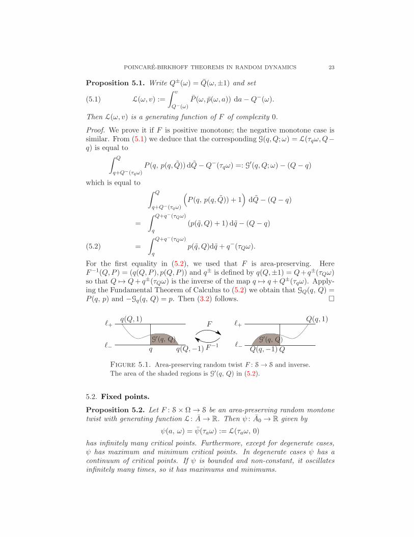
For the first equality in (5.2), we used that F is area-preserving. HereF−1(Q,P ) = (q(Q,P ), p(Q,P )) and q± is defined by q(Q,±1) = Q+ q±(τQω)so that Q 7→ Q+ q±(τQω) is the inverse of the map q 7→ q+Q±(τqω). Apply-ing the Fundamental Theorem of Calculus to (5.2) we obtain that GQ(q, Q) =P (q, p) and −Gq(q, Q) = p. Then (3.2) follows.
F
G′(q, Q)G′(q, Q)ℓ−ℓ−
ℓ+ℓ+
F−1q Q
q(Q, 1)
q(Q,−1)
Q(q, 1)
Q(q,−1)
Figure 5.1. Area-preserving random twist F : S → S and inverse.
The area of the shaded regions is G′(q, Q) in (5.2).
5.2. Fixed points.
Proposition 5.2. Let F : S× Ω → S be an area-preserving random montonetwist with generating function L : A→ R. Then ψ : A0 → R given by
ψ(a, ω) = ψ(τaω) := L(τaω, 0)
has infinitely many critical points. Furthermore, except for degenerate cases,ψ has maximum and minimum critical points. In degenerate cases ψ has acontinuum of critical points. If ψ is bounded and non-constant, it oscillatesinfinitely many times, so it has maximums and minimums.

24 ALVARO PELAYO FRAYDOUN REZAKHANLOU
Proof. We prove the last statement by contradiction. Suppose that ψ(a, ω)is monotone for large a. Then lima→∞ ψ(a, ω) = ψ(∞, ω) is well-defined.By ergodicity ψ(∞, ω) = ψ(∞) is independent of ω. On the other hand, forany bounded continuous function J : R → R we have that E J(ψ(a, ω)) =E J(ψ(ω)) for every a, and therefore J(ψ(∞)) = E J(ψ(ω)). Thus ψ(ω) =ψ(∞) a.s. In other words, if ψ(a, ω) doesn’t oscillate, then ψ(a, ω) is constant.
5.3. Construction of random monotone twists and spectral natureof fixed points. As we argued in Proposition 5.1, a monotone twist mapmay be determined in terms of its generating function. We now explain howwe can start from a scalar-valued function H(ω, v) and construct a monotonetwist map from it. To explain this construction, let us derive a useful propertyof generating functions. Recall Q±(ω) = Q(ω,±1).
Proposition 5.3. Let L(ω, v) be as in Proposition 5.1. Then the function
(5.3) L(ω,Q+(ω))−Q+(ω),
is constant and L(ω,Q−(ω)) = −Q−(ω).
Proof. From F (q,−Gq(q,Q;ω)) = (Q,GQ(Q, q;ω)), we deduce
F (ω,Lv(ω, v)− Lω(ω, v)) = (v,Lv(ω, v)).
Since P = ±1 if and only if p = ±1, we obtain Lω(ω,Q±(ω)) = 0 and
Lv(ω,Q±(ω)) = ±1. But
∇ω
(
L(ω,Q±(ω)))
= Lω(ω,Q±(ω)) + Lv(ω,Q
±(ω))Q±ω (ω) = ±Q±
ω (ω),
which means that the function L(ω,Q±(ω)) ∓ Q±(ω) is constant by the er-godicity of P. On the other hand, by the definition of L (see (5.1)) we knowthat L(ω,Q−(ω)) = −Q−(ω).
We are ready to give a recipe for constructing a monotone twist map froma C2 function H : Ω× R → R, which satisfy the following conditions
H(ω, 0) = 0, H(ω, a) > 0 for a > 0,
η(ω) = infa > 0 | H(ω, a) = 2 < +∞,(5.4)
almost surely. For such a function H, we set
σ(ω) = η(ω)−1
2
∫ η(ω)
0H(ω, a)da
and
Q−(ω) = −σ(ω), Q+(ω) = (η − σ)(ω);(5.5)
G(ω, v) = H(ω, v + σ(ω)), G(q,Q;ω) = G(τqω,Q− q);(5.6)
L(ω, v) =
∫ v+σ(ω)
0H(ω, a)da− v; G(q,Q;ω) = L(τqω,Q− q).
POINCARE-BIRKHOFF THEOREMS IN RANDOM DYNAMICS 25
Theorem 5.4. Assume that H : Ω×R → R satisfies (5.4) and the conditionGq < 0 with G defined as in (5.6). Then there exists a unique monotonetwist map F such that F (q,−Gq(q,Q)) = (Q,GQ(q,Q)), and F (q,±1) = (q +Q±(τqω),±1) with Q± defined by (5.5). Moreover, if q is a local maximum(respectively minimum) for q 7→ ψ(q) = G(q, q), then DF at the F -fixed point(q,−Gq(q, q)) has negative (respectively positive) eigenvalues.
Proof. By the definition,
G(q,Q) =
∫ Q
q+Q−(τqω)G(q,Q′) dQ′ − (Q− q),
which implies
GQ = G− 1, GQq = Gq < 0.(5.7)
From (5.7) we learn that the map Q 7→ Gq(q,Q) is decreasing and, as a result,the equation
Gq(q,Q) = −p(5.8)
may be solved for Q, to yield a p-increasing function Q = Q(q, p). We set
P (q, p) = GQ(q,Q(q, p)) = G(q,Q(q, p)) − 1,
so that
F (q, p) = (Q(q, p), P (q, p)).
Note that the monotonicity condition is satisfied because Q is increasing inp. We need to show that the boundary conditions are satisfied and thatF is area-preserving. For the latter, observe that by differentiating bothsides of the relationship (5.8), we obtain Gqq + GQqQq = 0, GqQQp = −1,Pq = GQq + GQQQq, and Pp = GQQQp. It follows that
(5.9) DF = −G−1Qq
[
Gqq 1GqqGQQ − G2
qQ GQQ
]
.
It follows from (5.9) that if the eigenvalues of DF are λ and λ−1, then λ > 0if and only if
Trace(DF ) =Gqq + GQQ
−GqQ= λ+ λ−1 > 2.
Equivalently DF has positive eigenvalues if and only if
ψ′′(q) = (Gqq + GQQ + 2GqQ)(q, q) > 0.
The case of negative eigenvalues may be treated in the same way.For the boundary conditions, we first establish
(5.10) Lω(ω,Q±(ω)) = 0, Lv(ω,Q
±(ω)) = ±1.
For the second equality in (5.10), observe that Lv = G− 1, and by definitionG(ω,Q−(ω)) = H(ω, 0) = 0, and G(ω,Q+(ω)) = H(ω,Q+(ω) − Q−(ω)) =
26 ALVARO PELAYO FRAYDOUN REZAKHANLOU
H(ω, η(ω)) = 2. As for the first equality in (5.10), observe that by the defini-tion of σ, G and L,
L(ω,Q−(ω)) +Q−(ω) = 0,
L(ω,Q+(ω))−Q+(ω) =
∫ Q+(ω)+σ(ω)
0H(ω, a)da− 2Q+(ω)
=
∫ η(ω)
0H(ω, a)da− 2(η − σ)(ω) = 0.
As a result
L(ω,Q±(ω))∓Q±(ω) = 0.(5.11)
Differentiating (5.11) with respect to ω yields
0 = Lω(ω,Q±(ω)) + Lv(ω,Q
±(ω))Q±ω (ω)∓Q±
ω (ω) = Lω(ω,Q±(ω)),
which is precisely the first equality in (5.10).We are now ready to verify the boundary conditions. We wish to show that
Q(q,±1) = q +Q±(τqω), or equivalently
±1 = −Gq(q, q +Q±(τqω)) = (Lv − Lω)(τqω,Q±(τqω)).
This is an immediate consequence of (5.10). It remains to verify P (q,±1) =±1. We certainly have
P (q,±1) = GQ(q, q +Q±(τqω)) = G(q, q +Q±(τqω))− 1 = G(τqω,Q±(τqω))− 1
This and (5.10) imply P (q,±1) = ±1, because G− 1 = Lv.
Remark 5.5. σ in (5.5) is motivated by (5.3). It is chosen so that L(ω,Q+(ω)) =Q+(ω).
Remark 5.6. The monotonicity condition Gq = GQq < 0 may be expressedas Hω(ω, a) < Ha(ω, a)(1−σ
′(ω)). The derivative of σ may be calculated withthe aid of (5.5):
σ′(ω) = η′(ω)−1
2H(ω, η(ω))η′(ω)−
1
2
∫ η(ω)
0Hω(ω, a)da
= −1
2
∫ η(ω)
0Hω(ω, a)da.
Example 5.7 We now give a concrete example of H that satisfies the as-sumptions of Theorem 8.4. Consider H(a, ω) = R(ω)a for R(q, ω) = R(τqω)a positive C1 stationary process. For such H, we have η = 2σ = 2R−1, andQ± = ±R−1. The condition Gq < 0 is equivalent to
(5.12) R′(Q− q)−R < 0.
for q,Q ∈ [Q−, Q+]. Eqivalently,
R′ > 0 ⇒ 2R′R−1 ≤ R,
R′ < 0 ⇒ −2R′R ≤ R.
POINCARE-BIRKHOFF THEOREMS IN RANDOM DYNAMICS 27
In summary, we need 2|R′| ≤ R2 to hold.
5.4. The density of fixed points. When F is a positive twist map, it hasa generating function G(q,Q, ω) = L(τqω,Q − q) and any fixed point of F isof the form (q0,Lv(τq0ω, 0)) where q0 is a critical point of the random processψ(q, ω) = ψ(τqω) (Propositions 3.3 and 5.1). We have also learned that anyrandom process ψ has infinitely many local maximums and minimums. In thissection we give sufficient conditions to ensure that such a random process hasa positive density of critical points, which in turn yields a positive density forfixed points of a monotone twist map. Let ♯B be the cardinality of a set B.
Definition 5.8. The density of A ⊂ R is den(A) := limℓ→∞ (2ℓ)−1♯(A ∩[−ℓ, ℓ]).
Let us state a set of assumptions for the random process ψ(q, ω) = ψ(τqω)that would guarantee the existence of a density for the set
Z(ω) := q | ψ′(q, ω) = 0.
Hypothesis 5.9. (i) ψ(q, ω) is twice differentiable almost surely and if
φℓ(δ;ω) = sup
|ψ′′(q, ω)− ψ′′(q, ω)| | q, q ∈ [−ℓ, ℓ], |q − q| 6 δ
,
then limδ→0 E φℓ(δ;ω) = 0 for every ℓ > 0.(ii) The random pair (ψω(ω), ψωω(ω)) has a probability density ρ(x, y). In
other words, for any bounded continuous function J(x, y),
EJ(ψ′(q, ω), ψ′′(q, ω)) =
∫
R
J(x, y) ρ(x, y) dxdy.
(iii) There exists ε > 0 such that ρ(x, y) is jointly continuous for x satis-fying |x| > ε.
We define Z±(ω) := q | ψ′(q, ω) = 0, ±ψ′′(q, ω) > 0 and N±ℓ (ω) :=
Z±(ω) ∩ [−ℓ, ℓ]. It is well known that if we assume Hypothesis 5.9, then
(5.13) E Nℓ(ω) = 2ℓ
∫
R
ρ(0, y)y± dy.
This is the celebrated Rice Formula and its proof can be found in [Ad00, Az09].Next we state a direct consequence of Rice Formula and the Ergodic Theorem.
Theorem 5.10. If ψ satisfies Hypothesis 5.9 then Z(ω) = Z(ω) almost surelyand
(5.14) limℓ→∞
E
∣
∣
∣
∣
1
2ℓN±
ℓ (ω)−
∫
R
ρ(0, y)y± dy
∣
∣
∣
∣
= 0.
Proof. Pick a smooth function ζ : R → [0,∞) such that its support iscontained in the interval [−1, 1], ζ(−a) = ζ(a), and
∫
Rζ(q)dq = 1. Set
ζε(q) := ε−1ζ(q/ε). It is not hard to show
(5.15)1
2ℓN±
ℓ (ω) >1
2ℓ
∫ ℓ−ε
−ℓ+ε
∣
∣
∣ζ ′ε ∗ ψ(q, ω)
∣
∣
∣dq =: X±
ε (ℓ, ω),
28 ALVARO PELAYO FRAYDOUN REZAKHANLOU
where ψ(q, ω) = 11(ψ′(q, ω) > 0) (this is [Az09, Lemma 3.2]). We note that if
ηε(ω) =∣
∣
∣
∫
Rζ ′ε(a)ψ(a, ω) da
∣
∣
∣, then
ηε(τqω) =
∣
∣
∣
∣
∫
R
ζ ′ε(a)ψ(a, τqω) da
∣
∣
∣
∣
=
∣
∣
∣
∣
∫
R
ζ ′ε(a)ψ(a+ q, ω) da
∣
∣
∣
∣
=∣
∣
∣ζ ′ε ∗ ψ(q)
∣
∣
∣.
From this and the Ergodic Theorem we deduce
(5.16) limℓ→∞
1
2ℓ
∫ ℓ
−ℓ
∣
∣
∣ζ ′ε ∗ ψ(q, ω)
∣
∣
∣dq = Eηε,
almost surely and in the L1(P) sense.On the other hand,
(5.17) limε→0
Eηε =
∫
R
ρ(0, y)y± dy =: X±.
This follows the proof of Rice Formula, see [Az09, proof of Theorem 3.4].Again by Rice Formula,
0 = E
[
1
2ℓN±
ℓ (ω)− X±
]
= E
[
1
2ℓN±
ℓ (ω)−X±ε (ℓ, ω)
]
− E[
X±ε (ℓ, ω)− X±
]
,
which implies
(5.18) limε→0
lim supℓ→∞
E
[
1
2ℓN±
ℓ (ω)−X±ε (ℓ, ω)
]
= 0,
because by (5.16) and (5.17),
(5.19) limε→0
lim supℓ→∞
E∣
∣X±ε (ℓ, ω)− X±
∣
∣ = 0.
From (5.15) and (5.18) we deduce
limε→0
lim supℓ→∞
E
∣
∣
∣
∣
1
2ℓN±
ℓ (ω)−X±ε (ℓ, ω)
∣
∣
∣
∣
= 0.(5.20)
Then (5.20) and (5.19) imply (5.14).
6. Complexity N = 1 area-preserving random twists
6.1. Domain of random generating functions. We begin by describingthe domain the random generating function of a complexity one twist.
Lemma 6.1. Let F be an area-preserving random twist of complexity one withdecomposition F = F1 F0, where F1 is a positive monotone area-preservingrandom twist and F0 is negative monotone area-preserving random twist. LetG0, G1 be the generating functions, respectively, of the monotone twists F0, F1.Then G1 := F−1
1 is a negative area-preserving random twist with generating
function given by G1(q, ξ) := −G1(ξ, q), and if
D0 := Domain(G0) and D1 := Domain(G1),(6.1)
POINCARE-BIRKHOFF THEOREMS IN RANDOM DYNAMICS 29
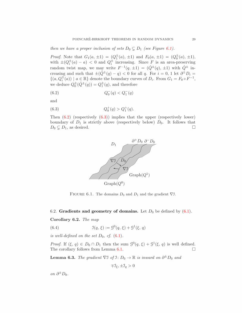
then we have a proper inclusion of sets D0 ( D1 (see Figure 6.1).
Proof. Note that G1(a, ±1) = (Q±1 (a), ±1) and F0(a, ±1) = (Q±
0 (a), ±1),with ±(Q±
i (a) − a) < 0 and Q±i increasing. Since F is an area-preserving
random twist map, we may write F−1(q, ±1) = (Q±(q), ±1) with Q± in-
creasing and such that ±(Q±(q) − q) < 0 for all q. For i = 0, 1 let ∂±Di =(a,Q∓
i (a)) | a ∈ R denote the boundary curves of Di. From G1 = F0 F−1,
we deduce Q±0 (Q
±(q)) = Q±1 (q), and therefore
Q−0 (q) < Q−
1 (q)(6.2)
and
Q+0 (q) > Q+
1 (q).(6.3)
Then (6.2) (respectively (6.3)) implies that the upper (respectively lower)boundary of D1 is strictly above (respectively below) D0. It follows thatD0 ( D1, as desired.
D0
D1
∇I
∇I
∂+D0 ∂−D0
Graph(Q0)
Graph(Q1)
Figure 6.1. The domains D0 and D1 and the gradient ∇I.
6.2. Gradients and geometry of domains. Let D0 be defined by (6.1).
Corollary 6.2. The map
I(q, ξ) := G0(q, ξ) + G1(ξ, q)(6.4)
is well-defined on the set D0, cf. (6.1).
Proof. If (ξ, q) ∈ D0 ∩ D1 then the sum G0(q, ξ) + G1(ξ, q) is well defined.The corollary follows from Lemma 6.1.
Lemma 6.3. The gradient ∇I of I : D0 → R is inward on ∂±D0 and
∓Iξ,±Iq > 0
on ∂±D0.
30 ALVARO PELAYO FRAYDOUN REZAKHANLOU
Proof. If F0(q, p) = (ξ, η) and F1(ξ, η′) = (q, P ), then Iq(q, ξ) = P − p
and Iξ(q, ξ) = η − η′ hold. We express the domain D0 of I given by (6.1)as (ξ, q) | p = p(q, ξ) = −G0
q(q, ξ) ∈ [−1, 1]. On ∂−D0, η = p = 1
and P, η′ < 1 (because D0 ( D1). So on ∂−D0 we have Iξ(q, ξ) > 0 andIq(q, ξ) < 0. On ∂+D0 we have η = p = −1 and η′, P < 1. So on ∂+D0
we have Iξ(q, ξ) < 0 and Iq(q, ξ) > 0. The lower boundary ∂−D0 is thegraph of an increasing function q 7→ h(q), and of course h′(q) > 0. So, thetangent to ∂−D0 is (1, h′(q)) and the inward normal is (−h′(q), 1). On ∂−D0
we have Iξ(q, ξ) > 0 and Iq(q, ξ) < 0. So we have that the dot product〈(Iq(q, ξ), Iξ(q, ξ)), (−h
′(q), 1)〉 = −h′(q)Iq(q, ξ) + Iξ(q, ξ) > 0. That is, onthe lower boundary ∇I is inward.
The case of the upper boundary is analogous.
6.3. Fixed points. If we set D := (q, a) | (q, q+a) ∈ D0, we have that, for
a pair of random processes B−(τqω), B+(τqω) > 0, D = (q, a) | −B−(τqω) <
a < B+(τqω). We then use the notation of Lemma 4.4 to set I(τqω, a) :=L0(τqω, a) +L1(τaτqω,−a) = I(q, q+ a). Define the map K : Ω× [−1, 1] → R
by
K(q, p;ω) = K(τqω, p) = I (τqω,B(τqω, p)) ,
where
B(τqω, p) =p+ 1
2B+(τqω) +
p− 1
2B−(τqω).
Note that
Kp(q, p;ω) =1
2Ia (τqω,B(τqω, p))
(
B+(τqω) +B−(τqω))
,
Kq(q, p;ω) =Iω (τqω,B(τqω, p)) + Ia (τqω,B(τqω, p))Bω(τqω, p).(6.5)
Hence there is a one-one correspondence between the critical points of K andI. From (6.5) and Lemma 6.3 we conclude the following.
Lemma 6.4. The gradient ∇K of K : S× Ω → R is inward on the boundaryof S.
Theorem 6.5. Let K : Ω× [−1, 1] → R be a C1-map such that ∓Kp(·,±1) >0. Let K(q, p;ω) := K(τqω, p).
(a) K has infinitely many critical points;(b) Furthermore, the critical points of K occur as follows:
(1) Either K has a continuum of critical points;(2) Or K has both infinitely many local maximums, and infinitely many
saddle points or local minimums.
Proof. We prove (b). If K(ω) := maxa∈[−1,1] K(ω, a), then either K is con-
stant or K(τqω) oscillates almost surely. In the former case for almost allω, there exists a(ω) such that K(ω, a(ω)) is a maximum and (of course)a(ω) /∈ −1, 1 by the assumption ∓Kp(·,±1) > 0. More concretely, we set
a(ω) = maxp ∈ [−1, 1] | K(ω, p) = K(ω).
POINCARE-BIRKHOFF THEOREMS IN RANDOM DYNAMICS 31
Hence K has a continuum of critical points of the form (q, a(τqω)) | q ∈R. In the latter case, there are infinitely many local maximums. Choose q
so that K(τqω) is a local maximum. For such (q, ω) choose a(τqω) so that
K(τqω, a(τqω)) = K(τqω). Therefore K has infinitely many local maximumsby Proposition 5.2.
Note that if
Ω0 :=
ω | τaω | a > a0 is dense for every a0
,
then P(Ω0) = 1. This is true because the family τa : a ∈ R is ergodic andby assumption P(U) > 0 for every open set U . Given ω ∈ Ω0, consider theordinary differential equation with initial value condition
q′(t) = Kω(τq(t)ω, p(t))
p′(t) = Kp(τq(t)ω, p(t))
q(0) = 0, p(0) = a.
(6.6)
There are two possibilities; the first possibility is that for some a, we havethat q(t) is unbounded as t → ∞, and in this case we claim that there isa continuum of critical points. The second possibility is that q(t) is alwaysbounded as t → ∞, and in this case we claim that K has either infinitelymany saddle points or local minimums. We proceed with case by case.Case 1 . (The map q(t) is unbounded as t → ∞ for some ω ∈ Ω0). We wantto prove that K has a continuum of critical points. Define ω(t) := τq(t)ω, andlet φr be the flow of (6.6). Note that
d
dtK(ω(t), p(t)) = |∇K(ω(t), p(t))|2 > 0.
Since q(t) is unbounded, ω(t) can approach almost any point in Ω. Moreoverif τq(tn)ω → ω and p(tn) → p, then we claim that ∇K(ω, p) = 0. Indeed, if
λ := supt>t0K(ω(t), p(t)), we have λ = K(ω, p), and since
λ = supt>t0
K(ω(t+ r), p(t+ r)),
we have, for any r > 0, that λ = K(ω, p) = K(φr(ω, p)). Hence ∇K(ω, p) =0; otherwise
d
drK(φr(ω, p))|r=0 > 0,
which is impossible. Note that ω could be any point in Ω and therefore forsuch ω there exists p = p(ω) such that ∇K(ω, p(ω)) = 0, i.e. we have acontinuum of critical points. This concludes Case 1.Case 2 . (The map q(t) = q(t, ω) is bounded for every ω ∈ Ω0). We claim thatif K does not have a continuum of fixed points, then K has infinitely manycritical points which are local minimums or saddle points. Suppose that thisis not the case, then we want to arrive at a contradiction. In order to do thislet x = (q, p) be a local maximum, which we know it always exists by theparagraphs preceding Case 1. In fact we may take a δ > 0 such that K(x) 6
32 ALVARO PELAYO FRAYDOUN REZAKHANLOU
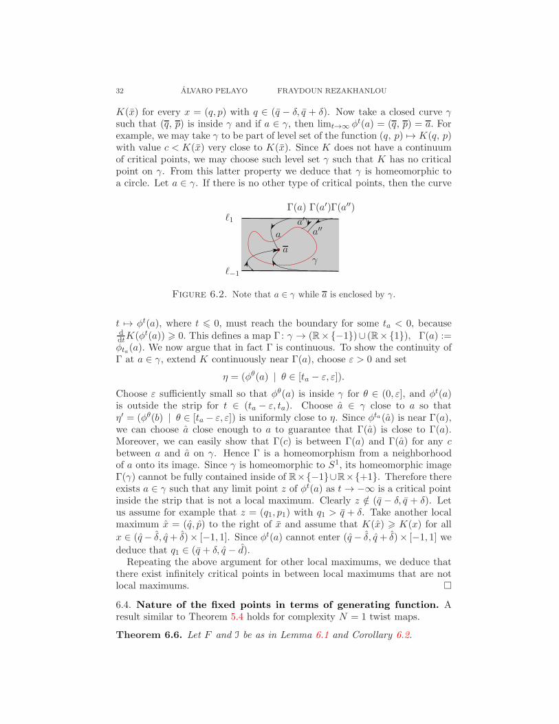
K(x) for every x = (q, p) with q ∈ (q − δ, q + δ). Now take a closed curve γsuch that (q, p) is inside γ and if a ∈ γ, then limt→∞ φt(a) = (q, p) = a. Forexample, we may take γ to be part of level set of the function (q, p) 7→ K(q, p)with value c < K(x) very close to K(x). Since K does not have a continuumof critical points, we may choose such level set γ such that K has no criticalpoint on γ. From this latter property we deduce that γ is homeomorphic toa circle. Let a ∈ γ. If there is no other type of critical points, then the curve
ℓ1
ℓ−1
a
a′
a′′
Γ(a) Γ(a′)Γ(a′′)
γa
Figure 6.2. Note that a ∈ γ while a is enclosed by γ.
t 7→ φt(a), where t 6 0, must reach the boundary for some ta < 0, becauseddtK(φt(a)) > 0. This defines a map Γ: γ → (R×−1)∪ (R×1), Γ(a) :=φta(a). We now argue that in fact Γ is continuous. To show the continuity ofΓ at a ∈ γ, extend K continuously near Γ(a), choose ε > 0 and set
η = (φθ(a) | θ ∈ [ta − ε, ε]).
Choose ε sufficiently small so that φθ(a) is inside γ for θ ∈ (0, ε], and φt(a)is outside the strip for t ∈ (ta − ε, ta). Choose a ∈ γ close to a so thatη′ = (φθ(b) | θ ∈ [ta − ε, ε]) is uniformly close to η. Since φta(a) is near Γ(a),we can choose a close enough to a to guarantee that Γ(a) is close to Γ(a).Moreover, we can easily show that Γ(c) is between Γ(a) and Γ(a) for any cbetween a and a on γ. Hence Γ is a homeomorphism from a neighborhoodof a onto its image. Since γ is homeomorphic to S1, its homeomorphic imageΓ(γ) cannot be fully contained inside of R×−1∪R×+1. Therefore thereexists a ∈ γ such that any limit point z of φt(a) as t → −∞ is a critical pointinside the strip that is not a local maximum. Clearly z /∈ (q − δ, q + δ). Letus assume for example that z = (q1, p1) with q1 > q + δ. Take another localmaximum x = (q, p) to the right of x and assume that K(x) > K(x) for all
x ∈ (q− δ, q+ δ)× [−1, 1]. Since φt(a) cannot enter (q − δ, q + δ)× [−1, 1] we
deduce that q1 ∈ (q + δ, q − d).Repeating the above argument for other local maximums, we deduce that
there exist infinitely critical points in between local maximums that are notlocal maximums.
6.4. Nature of the fixed points in terms of generating function. Aresult similar to Theorem 5.4 holds for complexity N = 1 twist maps.
Theorem 6.6. Let F and I be as in Lemma 6.1 and Corollary 6.2.
POINCARE-BIRKHOFF THEOREMS IN RANDOM DYNAMICS 33
Let (q, ξ) be a critical point of I and ~x be the corresponding fixed point ofF as in Proposition 3.3. Assume that Iξξ(q, ξ) 6= 0. Then DF (~x) has positive(respectively negative) eigenvalues if and only if det I(q, ξ) > 0 (respectively6 0).
Proof. Recall that S(q,Q; ξ) = S0(q, ξ) + S1(ξ,Q) and:
Gξ(q,Q; ξ) = 0 ⇒ F (q, −Gq(q,Q; ξ)) = (Q,GQ(q,Q; ξ)).
Observe that if cI(q, ξ) = cGξξ(q, q; ξ) 6= 0, then near (q, q, ξ), we can solveGξ(q,Q; ξ) = 0 as ξ = ξ(q,Q). Write T(q,Q) = G(q,Q; ξ(q,Q)). Then Tq =Gq, TQ = GQ, and F (q,−Tq(q,Q)) = (Q,TQ(q,Q)). As a result, we can show
DF =1
−TqQ
[
Tqq 1TqqTQQ − T2
qQ TQQ
]
,
in the same way we derived (5.9). Observe that Trace(DF ) =Tqq+TQQ
−TqQ. Since
Tqq = Gqq + Gqξξq, TQQ = GQQ + GQξξQ, TqQ = GqQ + GqξξQ, and TQq =GQq + GQξξq, we have that
Tqq + TQQ + 2TqQ = Gqq + GQQ + 2GqQ + (Gqξ + GQξ)(ξq + ξQ).
On the other hand, by differentiating the relationship Gξ(q,Q; ξ(q,Q)) = 0,
we have Gξq + Gξξξq = 0 and GξQ + GξξξQ = 0, or equivalently, ξq = −Gξq
Gξξ,
ξQ = −GξQ
Gξξ. In particular, Gξq +GξQ +Gξξ(ξq + ξQ) = 0, which in turn implies
Tqq + TQQ + 2TqQ = Gqq + GQQ + 2GqQ −1
Gξξ(Gqξ + GQξ)
2.
Furthermore, if I(q, ξ) = G(q, q; ξ), then Iq = Gq + GQ, Iξ = Gξ, and
D2I =
[
Gqq + GQQ + 2GqQ GξQ + Gξq
GξQ + Gξq Gξξ
]
.
So Tqq + TQQ + 2TqQ = det(D2I)Gξξ
. Also, TqQ = GqQ −GqξGQξ
Gξξ. Now
Trace(DF ) − 2 =Tqq + TQQ + 2TqQ
−TqQ=
det(D2I)
GqQGξξ − GqξGQξ.(6.7)
Recall G(q,Q; ξ) = G0(q, ξ) + G1(ξ,Q) with G0qξ > 0, and G1
Qξ < 0 because F 0
is a negative monotone twist and F 1 is a positive monotone twist. Hence weobtain −GqξGQξ > 0. On the other hand GqQ = 0, which simplifies (6.7) to
Trace(DF )− 2 =Tqq + TQQ + 2TqQ
−TqQ=
det(D2I)
−GqξGQξ.
This expression has the same sign as det(D2I). Finally DF has positive eigen-values if and only if Trace(DF ) > 2, if and only if det(D2I) ≥ 0, whichconcludes the proof.
34 ALVARO PELAYO FRAYDOUN REZAKHANLOU
7. Complexity N = 2 area-preserving random twists
7.1. Domain of random generating functions. Next we describe the do-main of a random generating function associated to a complexity N = 2 twist.
Lemma 7.1. Let F be an area-preserving random twist of complexity N = 2.Suppose that F decomposes as F = F2F1F0, where F1 is a positive monotonearea-preserving random twist and Fj is negative monotone area-preservingrandom twist for j = 0, 2. Let G0,G1,GN be the corresponding generatingfunctions. Write Gi = F−1
i and define Q±i and Q±
i by Fi(q,±1) = (Q±i (q),±1)
and Gi(q,±1) = (Q±i (q),±1). Then the function I(q, ξ1, ξ2) := G0(q, ξ1) +
G1(ξ1, ξ2) + G2(ξ2, q), is well-defined on the set
D =
(q, ξ1, ξ2) | Q+0 (q) 6 ξ1 6 Q−
0 (q), Q−2 (q) 6 ξ2 6 Q+
2 (q)
,
Moreover, if (q, ξ1, ξ2) ∈ D, then Q−1 (ξ1) < ξ2 < Q+
1 (ξ1).
Proof. Since F1 = G2 F G0, we have
(7.1) Q±2 Q± Q±
0 = Q±1 ,
where Q± are defined by the relationship F (q,±1) = (Q±(q),±1). On theset D, G0(q, ξ1) and G2(ξ2, q) are well defined. It is sufficient to check that if(q, ξ1, ξ2) ∈ D, then G1(ξ1, ξ2) is well-defined. That is, Q
−1 (ξ1) < ξ2 < Q+
1 (ξ1).To see this observe that by (7.1),
±Q±1 (ξ1) = ±
(
Q±2 Q± Q±
0
)
(ξ1) > ±(
Q±2 Q±
)
(q) > ±Q±2 (q) > ±ξ2,
as desired. Here for the first inequality we used the fact that Q± and Q±2
are increasing and that in D, we have Q−0 (ξ1) 6 q 6 Q+
0 (ξ1); for the secondinequality we used ±Q±(q) > ±q, which concludes the proof.
We define B±0 (ω), B
±2 (ω) > 0, by Q±
0 (q) = q ∓ B±0 (τqω) and Q±
2 (q) =q ±B±
2 (τqω). Let
K(q, p;ω) = K(τqω, p) = I(q, ξ(q, p)) = I(τqω, q + ξ(τqω, p)),(7.2)
where p = (p1, p2), ξ(ω, p) = (ξ1(ω, p1), ξ2(ω, p2)), ξ(q, p) = (q+ξ1(τqω, p1), q+
ξ2(τqω, p2)), and ξ1 and ξ2 are defined by ξ1(ω, p1) :=p1+12 B−
0 (ω)+p1−12 B+
0 (ω)
and ξ2(ω, p2) :=p2+12 B+
2 (ω) +p2−12 B−
2 (ω).
Lemma 7.2. Let K : R× [−1, 1]2×Ω → R be as in (7.2). The following hold:
(i) There exists a one-to-one correspondence between critical points of I andK.
(ii) The vector ∇K is pointing inward on the boundary of R× [−1, 1]2.
POINCARE-BIRKHOFF THEOREMS IN RANDOM DYNAMICS 35
Proof. Evidently K(q, p1, p2) = K(q, p;ω) satisfies
Kp1(q, p1, p2) =12Iξ1(q, ξ(q, p))
(
B+0 +B−
0
)
(τqω),Kp2(q, p1, p2) =
12Iξ2(q, ξ(q, p))
(
B+2 +B−
2
)
(τqω),Kq(q, p1, p2) = Iq(q, ξ(q, p)) + Iξ1(q, ξ(q, p)) + Iξ2(q, ξ(q, p))
+Iξ1(q, ξ(q, p))(
p1+12 ∇B−
0 + p1−12 ∇B+
0
)
(τqω)
+Iξ2(q, ξ(q, p))(
p1+12 ∇B−
2 + p1−12 ∇B+
2
)
(τqω).
(7.3)
It follows from (7.3) that there exists a one-to-one correspondence betweenthe critical points of I and K because B±
i > 0 for i = 0, 2. This proves (i).We now examine the behavior of K across the boundary. Observe that the
functionsKp1 and Iξ1 (respectivelyKp2 and Iξ2) have the same sign. Moreover,
p1 = ±1 ⇔ ξ1 = Q∓0 (q),
p2 = ±1 ⇔ q = Q±2 (ξ2).
It remains to verify
ξ1 = Q∓0 (q) ⇒ ±Iξ1 < 0,
q = Q±2 (ξ2) ⇒ ±Iξ2 < 0.
Let us write ξ0 for q and ξ3 for Q. We define functions pi(ξi, ξi+1) andP i(ξi, ξi+1) by F i
(
ξi, pi(ξi, ξi+1)
)
=(
ξi+1, Pi(ξi, ξi+1)
)
. We then have Iξ1 =
G0Q + G1
q = P 0 − p1 and Iξ2 = G1Q + G2
q = P 1 − p2. Finally we assert,
p1 = ±1 ⇒ ξ1 = Q∓0 (q) ⇒ p0 = P 0 = ∓1 ⇒ ±Iξ1 < 0,
p2 = ±1 ⇒ ξ2 = Q±2 (q) ⇒ p2 = P 2 = ±1 ⇒ ±Iξ2 < 0,
as desired. Here we are using the fact that if p0 = P 0 = ∓1 or p2 = P 2 = ±1,then Q−
1 (ξ1) < ξ2 < Q+1 (ξ1) or equivalently p
1, P 1 /∈ −1, 1.
7.2. Fixed points. The following proof is sketched because it is similar tothat of Theorem 6.5.
Theorem 7.3. Let K : R × [−1, 1]2 × Ω → R, and K(q, p;ω) := K(τqω, p)be C1 up to the boundary with ∇K pointing inwards on the boundary. Then
(a) K has infinitely many critical points.(b) The critical points of K occur as follows:
(1) Either K has a continuum of critical points;(2) Or K has both infinitely many local maximums, and infinitely many
saddle points or local minimums.
Proof. We prove (b). As in the proof of Theorem 6.5, we assume that Kdoes not have a continuum of critical points and deduce that K has infinitelymany isolated local maximums. The q component of the flow remains boundedalmost surely. We take a local maximum a and a connected component γ ofa level set of K associated with a regular value c of K, very close to the valueK(a). The surface γ is an oriented closed manifold and if K has no other type
36 ALVARO PELAYO FRAYDOUN REZAKHANLOU
of critical point, then Γ : γ → R×∂[−1, 1]2, is a homeomorphism from γ ontoits image. Since the set R× ∂[−1, 1]2 cannot contain a homeomorphic imageof γ, we arrive at a contradiction. From this we deduce the conclusion of thetheorem as in the proof of Theorem 6.5.
8. Complexity N > 3 area-preserving random twists
8.1. Geometry of the domain of the generating function. Let F bean area-preserving random twist of complexity N . As in Theorem F, weassume that N is an odd number and that F decomposes as in (2.6). Recallthat G0, . . . ,GN denote the generating functions, respectively, of the monotonetwists F0, . . . , FN . Set
I(q, ξ) = G(q, q; ξ) = L(τqω, 0; ξ − q), I′(q, η) = I(q, η + q) =: I(τqω, η),
where G and L are defined by Lemma 4.4, and η + q = (η1 + q, . . . , ηN + q).Given a realization ω, we write D = D(ω) for the domain of the definitionof I. We also set D′(ω) = η ∈ RN | (0, η) ∈ D(ω) so that the domain ofthe function I′ is exactly (q, η) | η ∈ D′(τqω). To simplify the notation, wewrite ξ0 for q and ξN+1 for Q. In this way, we can write
F i(ξi, pi) = (ξi+1, P
i),
where
pi = pi(ξi, ξi+1) = −Giq(ξi, ξi+1)
and
P i = P i(ξi, ξi+1) = GiQ(ξi, ξi+1).
Here by Giq and Gi
Q we mean the partial derivatives of Gi with respect to its
first and second arguments respectively. As before, we write Gi for the inverseof F i and define increasing functions Q±
i and Q±i by F i(q,±1) = (Q±
i (q),±1)
and Gi(q,±1) = (Q±i (q),±1). Let
E(ξ1, ξN ) =
N−1⋂
i=1
(ξ2, . . . , ξN−1) | (−1)i+1Q−i (ξi) 6 (−1)i+1ξi+1 6 (−1)i+1Q+
i (ξi)
.
Then the set D consists of points (q, ξ) such that ξ1 ∈ [Q+0 (q), Q
−0 (q)], ξN ∈
[Q+N (q), Q−
N (q)] and (ξ2, . . . , ξN−1) ∈ E(ξ1, ξN ). Alternatively, we can write
E(ξ1, ξN ) =N−1⋂
i=1
(ξ2, . . . , ξN−1) | − 1 6 pi(ξi, ξi+1), Pi(ξi, ξi+1) 6 1
.
POINCARE-BIRKHOFF THEOREMS IN RANDOM DYNAMICS 37
We write ∂D = ∂+D ∪ ∂−D, where ∂+D and ∂−D represent the upper andlower boundaries of D. Then ∂+D =
⋃Ni=0 ∂
+i D and ∂−D =
⋃Ni=0 ∂
−i D, where
∂±0 D =
(q, ξ) ∈ D | ξ1 = Q∓0 (q)
=
(q, ξ) ∈ D | p0(q, ξ1) = P 0(q, ξ1) = ∓1
,
∂±ND =
(q, ξ) ∈ D | ξN = Q∓N (q)
=
(q, ξ) ∈ D | pN (ξN , q) = PN (ξ1, q) = ∓1
,
∂±i D =
(q, ξ) ∈ D | ξi+1 = Q±i (ξi)
for i odd and 1 < i < N,
∂±i D =
(q, ξ) ∈ D | ξi = Q±i (ξi+1)
for i even and 1 < i < N.
We also write ∂iD = ∂+i D ∪ ∂−i D, ∂±i D = ∂±i D \(
∂±i−1D ∪ ∂±i D)
, ∂±0 D =
∂±0 D \(
∂±1 D ∪ ∂±ND)
, ∂±ND = ∂±ND \(
∂±0 D ∪ ∂±N−1D)
.
8.2. The gradient. Next examine the behavior of ∇I across the boundary.The randomness of D(ω) and I play no role and the proof is analogous in theperiodic case ([Go01]).
Proposition 8.1. Let F = FN · · · F1 F0 be an area-preserving randomtwist decomposition as in (2.6). Then the following properties hold.
(P.i) If 1 < i < N is even, ∇I is inward along ∂±i D;
(P.ii) If 1 < i < N is odd, ∇I is outward along ∂±i D;
(P.iii) ∇I is outward along ∂±ND;
(P.iv) ∇I is inward along ∂±0 D.
Proof. Evidently, Iq(q, ξ) = PN−p0 and Iξi(q, ξ) = P i−1−pi, for i = 1, . . . , N .We wish to study the behavior of the function I across the boundary of D.On ∂±0 D, we have p0 = P0 = ∓1. Since Iξ1 = P 0 − p1, we deduce
(8.1) ± Iq > 0, ±Iξ1 < 0 on ∂±0 D.
On ∂±ND, we have pN = PN = ∓1. Since IξN = PN−1 − pN , we deduce
(8.2) ± IξN−1< 0, ±IξN > 0 on ∂±ND.
On ∂±i D we have P i = pi = ±(−1)i+1; hence±(−1)iIξi(q, ξ) = ±(−1)i(P i−1−pi) > 0 and ±(−1)iIξi+1
(q, ξ) = ±(−1)i(P i − pi+1) 6 0 if 1 < i < N . The
inequalities are strict on ∂±i D.The boundary ∂±0 D is the set of points (q, ξ) such that ξ1 = Q∓
0 (q) with
q 7→ Q∓0 (q) increasing. So, if we write Q
∓0 (q) for the derivative of Q∓
0 (q), then
any vector that has (1, Q∓0 (q)) for its projection onto (q, ξ1)-space would be
tangent to ∂±0 D. Hence a vector n0 that has ±(Q∓0 (q), −1) for the first two
components and 0 for the other components, is an inward normal vector tothe ∂±0 D part of boundary. As a result, we have that on ∂±0 D
〈∇I, n0〉 = ±(
Q∓0 (q)Iq − Iξ1
)
> 0,
by (8.1). Here 〈·, ·〉 denotes the dot product. That is, on ∂±0 D, the gradient∇I is inward, proving (P.iv). Similarly we use (8.2) to establish (P.iii).
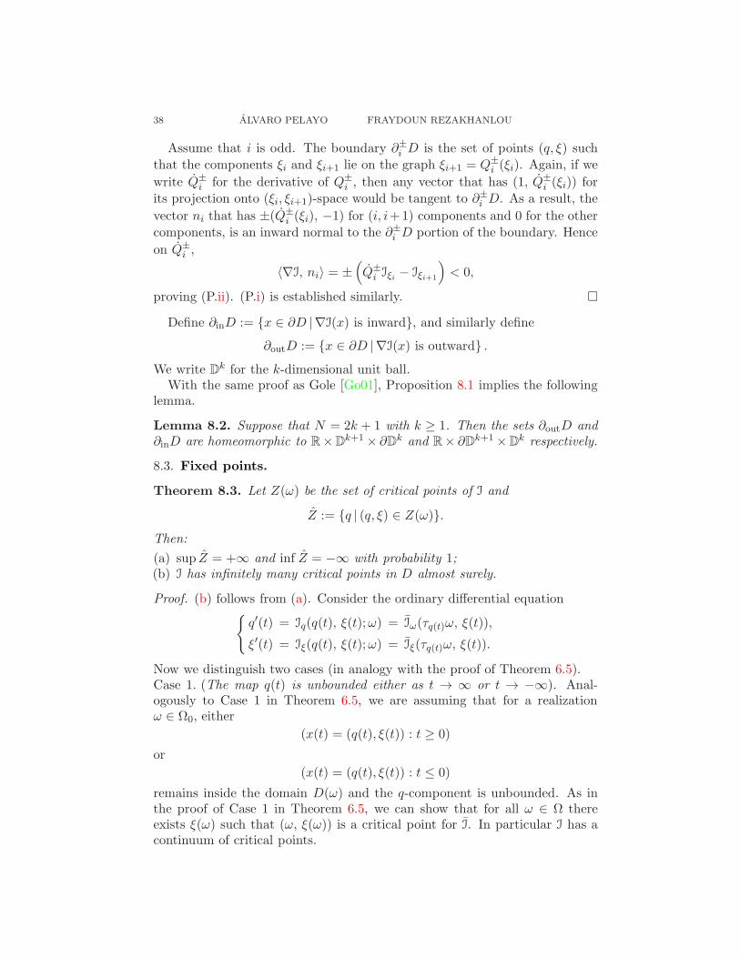
38 ALVARO PELAYO FRAYDOUN REZAKHANLOU
Assume that i is odd. The boundary ∂±i D is the set of points (q, ξ) such
that the components ξi and ξi+1 lie on the graph ξi+1 = Q±i (ξi). Again, if we
write Q±i for the derivative of Q±
i , then any vector that has (1, Q±i (ξi)) for
its projection onto (ξi, ξi+1)-space would be tangent to ∂±i D. As a result, the
vector ni that has ±(Q±i (ξi), −1) for (i, i+1) components and 0 for the other
components, is an inward normal to the ∂±i D portion of the boundary. Hence
on Q±i ,
〈∇I, ni〉 = ±(
Q±i Iξi − Iξi+1
)
< 0,
proving (P.ii). (P.i) is established similarly.
Define ∂inD := x ∈ ∂D |∇I(x) is inward, and similarly define
∂outD := x ∈ ∂D |∇I(x) is outward .
We write Dk for the k-dimensional unit ball.With the same proof as Gole [Go01], Proposition 8.1 implies the following
lemma.
Lemma 8.2. Suppose that N = 2k + 1 with k ≥ 1. Then the sets ∂outD and∂inD are homeomorphic to R×Dk+1 × ∂Dk and R× ∂Dk+1 ×Dk respectively.
8.3. Fixed points.
Theorem 8.3. Let Z(ω) be the set of critical points of I and
Z := q | (q, ξ) ∈ Z(ω).
Then:
(a) sup Z = +∞ and inf Z = −∞ with probability 1;(b) I has infinitely many critical points in D almost surely.
Proof. (b) follows from (a). Consider the ordinary differential equation
q′(t) = Iq(q(t), ξ(t);ω) = Iω(τq(t)ω, ξ(t)),
ξ′(t) = Iξ(q(t), ξ(t);ω) = Iξ(τq(t)ω, ξ(t)).
Now we distinguish two cases (in analogy with the proof of Theorem 6.5).Case 1. (The map q(t) is unbounded either as t → ∞ or t → −∞). Anal-ogously to Case 1 in Theorem 6.5, we are assuming that for a realizationω ∈ Ω0, either
(x(t) = (q(t), ξ(t)) : t ≥ 0)
or
(x(t) = (q(t), ξ(t)) : t ≤ 0)
remains inside the domain D(ω) and the q-component is unbounded. As inthe proof of Case 1 in Theorem 6.5, we can show that for all ω ∈ Ω thereexists ξ(ω) such that (ω, ξ(ω)) is a critical point for I. In particular I has acontinuum of critical points.
POINCARE-BIRKHOFF THEOREMS IN RANDOM DYNAMICS 39
Case 2. (The map q(t) is always bounded as t → ±∞). We want to showthat I has critical points strictly inside of D = D(ω). Let us first assume bycontradiction that I has no critical point inside of D(ω) for a realization of ω.Consider the flow
φt(q, ξ) := (q(t), ξ(t)) = x(t),
which starts at the point x = (q, ξ) ∈ ∂inD. Since q(t) stays bounded and weare assuming that there is no critical point inside, the flow must exit at somepositive time e(x). Write φ(x) = φe(x)(x). Note that the sets ∂inD and ∂outD
are open relative to ∂D. We now argue that the function φ(x) is continuous.
For example, φ is continuous at x Simply because we may extend I near φ(x)across the boundary so that for some small ε > 0, the flow φt(x) is well-definedand lies outside D for t ∈ (e(x), e(x)+ε). We can then guarantee that φt(y) isclose to φt(x) for t ∈ [0, e(x) + ε) and y sufficiently close to x. As a result, for
y sufficiently close to x, the point φe(y)(y) is close to φe(x)(x), concluding the
continuity of φ. In fact by interchanging ∂outD with ∂inD, we can show thatφ−1 is continuous. As a result φ is a homeomorphism from ∂inD onto ∂outD.This is impossible because ∂inD is not homeomorphic to ∂outDby Lemma 8.2.Hence I has at least one critical point in Int(D) and Z(ω) 6= ∅.
It remains to show that the set Z(ω) is unbounded on both sides. We onlyverify the unboundedness from above as the boundedness from below can beestablished in the same way. Suppose to the contrary that Z(ω) is boundedabove with positive probability. Since
(8.3) Z(τqω) = τ−qZ(ω) = (a− q, ξ) | (a, ξ) ∈ Z(ω),
by stationarity, we learn that the set Z(ω) is bounded above almost surely.Define x(ω) = (q(ω), ξ(ω)) by
q(ω) = maxq | (q, ξ) ∈ Z(ω)
and
ξ(ω) = maxξ | (q(ω), ξ) ∈ Z(ω).
Again by (8.3), q(τaω) + a = q(ω) and ξ(τaω) = ξ(ω), for every a ∈ R. As aresult,
P(
q(ω) > ℓ)
= P(
q(τaω) + a > ℓ)
= P(
q(τaω) > ℓ− a)
= P(
q(ω) > ℓ− a)
,
for every a and ℓ. Since this is impossible unless q = ∞, we deduce that theset Z(ω) is unbounded from above.
Acknowledgements. We thank Atilla Yilmaz for discussions, and Barney Bramhamand Kris Wysocki for comments on a preliminary version. AP is supportedby NSF grants DMS-1055897, DMS-1518420, and DMS-0635607, a J. TinselyOden Faculty Fellowship from the University of Texas, and an OberwolfachLeibniz Fellowship. He is grateful to the Institute for Advanced Study forproviding an excellent research environment for his research (December 2010 –September 2013), and to Helmut Hofer for fruitful discussions on many topics.
40 ALVARO PELAYO FRAYDOUN REZAKHANLOU
During the preparation of some parts of this paper he was hosted by Luis Caf-farelli, Alessio Figalli, and J. Tinsley Oden at the Institute for ComputationalSciences and Engineering in Austin, and he is thankful for the hospitality. FRis supported in part by NSF Grant DMS-1106526 and DMS-1407723. Partsof this paper were written during visits of AP to UC Berkeley and FR to theInstitute for Advanced Study and Washington University between 2010 and2013. Thanks to Tejas Kalelkar for help drawing some of the figures. Finally,we are grateful to the referee for helpful expository suggestions to make thepaper accessible to a wider audience.
Dedication . The authors dedicate this article to Alan Weinstein, whose fun-damental and deep insights in so many areas of geometry are a continuoussource of inspiration.
References
[Ad00] R. Adler and J.E. Taylor: Random Fields and Geometry. Springer Monographs inMathematics. Springer, New York, 2007.
[AFFHO12] P. Albers, J. Fish, U. Frauenfelder, H. Hofer, O. van Koert: Global surfaces ofsection in the planar restricted 3-body problem. Arch. Ration. Mech. Anal. 204 (2012)273-284.
[Ar78] V.I. Arnol’d: Mathematical Methods of Classical Mechanics, Springer-Verlag, Berlinand NY, 1978.
[AA68] V. I. Arnol’d and A. Avez: Ergodic Problems of Classical Mechanics, Benjamin,New York, 1968.
[Au13] M. Audin: Vladimir Igorevich Arnold and the inven-tion of symplectic topology, version de janvier 2013. athttp://www-irma.u-strasbg.fr/~maudin/mathematiques.html
[Az09] J. Azais and M. Wschebor: Level Sets and Extrema of Random Processes and Fields.John Wiley and Sons, Inc., Hoboken, NJ, 2009.
[BG97] J. Barrow-Green: Poincare and The Three Body Problem. History of Mathematics,11. American Mathematical Society, Providence, RI; London Mathematical Society,London, 1997. xvi+272 pp.
[Bi13] G. D. Birkhoff: Proof of Poincare’s last geometric theorem, Trans. AMS 14 (1913)14-22.
[Bi17] G. D. Birkhoff: Dynamical systems with two degrees of freedom, Trans. AMS 18
(1917) 199-300.[Bi26] G. D. Birkhoff: An extension of Poincare’s last geometric theorem, Acta. Math. 47
(1926) 297-311.[Bi66] G. D. Birkhoff: Dynamical Systems. With an addendum by Jurgen Moser. American
Mathematical Society Colloquium Publications, Vol. IX Amer. Math. Soc., Providence,R.I. 1966 xii+305 pp.
[BH12] B. Bramham and H. Hofer, First steps towards a symplectic dynamics, Surveys inDifferential Geometry 17 (2012) 127-178.
[BN77] L. E. J. M. Brown and W. D. Newmann: Proof of the Poincare-Birkhoff fixed pointtheorem, Michigan. Math. J. 24 (1977) 21-31.
[Br94] A. D. Bruno: The Restricted 3-Body Problem: Plane Periodic Orbits. Translated
from the Russian by Balint Erdi. With a preface by Victor G. Szebehely. de GruyterExpositions in Mathematics, 17. Walter de Gruyter & Co., Berlin, 1994. xiv+362 pp.
POINCARE-BIRKHOFF THEOREMS IN RANDOM DYNAMICS 41
[Ca82] P. H. Carter: An improvement of the Poincare-Birkhoff fixed point theorem, Trans.AMS 269 (1982) 285-299.
[Ch84] M. Chaperon: Une idee du type “geodesiques brisees” pour les systemes hamiltoniens.(French) [A ”broken geodesic” method for Hamiltonian systems] C. R. Acad. Sci. ParisSer. I Math. 298 (1984), no. 13, 293-296.
[Ch84b] M. Chaperon: An elementary proof of the Conley-Zehnder theorem in symplecticgeometry. Dynamical systems and bifurcations (Groningen, 1984), 1–8, Lecture Notesin Math., 1125, Springer, Berlin, 1985.
[Ch89] M. Chaperon: Recent results in symplectic geometry. Dynamical systems and ergodictheory (Warsaw, 1986), 143–159, Banach Center Publ., 23, PWN, Warsaw, 1989.
[CZ83] C.C. Conley and E. Zehnder: The Birkhoff-Lewis fixed point theorem and a conjec-ture of V. I. Arnol’d. Invent. Math. 73 (1983) 33-49.
[Di83] W.-Y. Ding : A generalization of the Poincare-Birkhoff theorem, Proc. AMS 88
(1983) 341-346.[Do53] J.L. Doob: Random Processes. John Wiley and Sons, Inc., New York; Chapman and
Hall, Limited, London, 1953. viii+654 pp.[DV80] D.J. Daley and D. Vere-Jones: A Introduction to the Theory of Point Processes.
Springer Series in Statistics, 1988.[Ei56] A. Einstein: Investigations on the theory of the Brownian movement. Edited with
notes by R. Furth. Translated by A. D. Cowper. Dover Publ., Inc., New York, 1956.vi+122 pp.
[Fl88] A. Floer: Morse theory for Lagrangian intersections. J. Diff. Geom. 28 (1988) 513-547.
[Fl89] A. Floer: Witten’s complex and infinite-dimensional Morse theory. J. Diff. Geom. 30(1989) 207-221.
[Fl89b] A. Floer: Symplectic fixed points and holomorphic spheres. Comm. Math. Phys.120 (1989) 575-611.
[Fl91] A. Floer: Elliptic methods in variational problems. A plenary address presented atthe International Congress of Mathematicians held in Kyoto, August 1990. ICM-90.Mathematical Society of Japan, Tokyo; distributed outside Asia by the AmericanMathematical Society, Providence, RI, 1990.
[Fr88] J. Franks: Generalizations of the Poincare-Birkhoff theorem, Ann. Math. (2) 128
(1988) 139-151.[Fr88b] J. Franks: Recurrence and fixed points of surface homeomorphisms. Ergodic Theory
Dynam. Systems 8 (1988), Charles Conley Memorial Issue, 99-107.[Fr06] J. Franks: Erratum to “Generalizations of the Poincare-Birkhoff theorem”, Ann.
Math. 164 (2006) 1097-1098.[GK11] J. Galante and V. Kaloshin: Destruction of invariant curves in the restricted circular
planar three-body problem by using comparison of action, Duke Math. J. 159 (2011)275-327.
[Go01] C. Gole: Symplectic Twist Maps. Global Variational Techniques. Advanced Seriesin Nonlinear Dynamics, 18. World Scient. Publis. Co., Inc., River Edge, NJ, 2001.xviii+305 pp.
[Gu94] L. Guillou: Theoreme de translation plane de Brouwer et generalisations du theoremede Poincare-Birkhoff, Topology 33 (1994) 331-351.
[Ho85] H. Hofer: Lagrangian embeddings and critical point theory. Ann. Inst. H. PoincareAnal. Non Lineaire 2 (1985) 407-462.
[Ho12] H. Hofer: Arnold and Symplectic Geometry, Not. AMS 59 (2012) 499-502.[HS95] H. Hofer and D. Salamon: Floer homology and Novikov rings. The Floer Memorial
Volume, 483-524, Progr. Math., 133, Birkhauser, Basel, 1995.[HWZ03] H. Hofer, K. Wysocki, and E. Zehnder: Finite energy foliations of tight three-
spheres and Hamiltonian dynamics, Ann. Math 157 (2003) 125-257.
42 ALVARO PELAYO FRAYDOUN REZAKHANLOU
[HZ94] H. Hofer and E. Zehnder: Symplectic Invariants and Hamiltonian Dynamics,Birkhauser, Basel (1994).
[Ja76] H. Jacobowitz: Periodic solutions of x′′ + f(x, t) = 0 via the Poincare-Birkhoff theo-rem, J. Diff. Equations 20 (1976) 37-52.
[Ja77] H. Jacobowitz: Corrigendum: The existence of the second fixed point: a correctionto Periodic solutions of x′′ + f(x, t) = 0 via the Poincare-Birkhoff theorem, J. Diff.Equations 25 (1977) 148-149.
[KH95] A. Katok and B. Hasselblatt: Introduction to The Modern Theory of Dynamical Sys-tems. With a supplem. chapter by Katok and L. Mendoza. Encyclopedia of Mathemat-ics and its Applications, 54. Cambridge University Press, Cambridge, 1995. xviii+802pp.
[Ko57] A. N. Kolmogorov: Theorie generale des systemes dynamiques et mecanique clas-sique, Proc. Internat. Congr. Math. (Amsterdam, 1954), Vol. 1, North-Holland, Ams-terdam, 1957, pp. 315-333.
[Le91] P. Le Calvez: Proprietes dynamiques des diffeomorphismes de l’anneau et du tore,Asterisque No. 204 (1991) 131 pp. Translation: Dynamical Properties of Diffeomor-phisms of the Annulus and of the Torus. Translated from the 1991 French originalby Philippe Mazaud. SMF/AMS Texts and Monographs, 4. Amer. Math. Soc., Prov-idence, RI; Societe Mathematique de France, Paris, 2000. x+105 pp.
[Le10] P. Le Calvez and J. Wang: Some remarks on the Poincare-Birkhoff theorem, Proc.AMS 138 (2010) 703-715.
[LT98] G. Liu and G. Tian: Floer homology and Arnol’d conjecture. J. Differential Geom.49 (1998) 1-74.
[Ma86] J. N. Mather: Dynamics of area-preserving maps. Proceedings of the Intern. Con-gress of Math., Vol. 1, 2 (Berkeley, Calif., 1986), 1190-1194, Amer. Math. Soc., Prov-idence, RI, 1987.
[MS98] D. McDuff and D. Salamon: Introduction to Symplectic Topology. Second edition.Oxford Mathematical Monographs. The Clarendon Press, Oxford University Press,New York, 1998. x+486 pp.
[Mo73] J. Moser: Stable and random motions in dynamical systems, Ann. of Math. Studies,no. 77, Princeton Univ. Press, Princeton, N.J., and Univ. of Tokyo Press, Tokyo, 1973.
[Ne67] E. Nelson: Dynamical Theories of Brownian motion. Princeton University Press,Princeton, N.J. 1967 iii+142p.
[Ne77] W.D. Neumann: Generalizations of the Poincare Birkhoff fixed point theorem, Bull.Austral. Math. Soc. 17 (1977) 375-389.
[On95] K. Ono: On the Arnol’d conjecture for weakly monotone symplectic manifolds,Invent. Math. 119 (1995) 519-537.
[Po93] H. Poincare: Les Methodes Nouvelles de la Mecanique Celeste, Tome I, Paris,Gauthier-Viltars, 1892. Republished by Blanchard, Paris, 1987.
[Po12] H. Poincare: Sur un theoreme de geometrie, Rend. Circ. Mat. Palermo 33 (1912)375-407.
[Pol01] L. Polterovich: The Geometry of the Group of Symplectic Diffeomorphisms. Lecturesin Mathematics ETH Zurich. Birkhauser Verlag, Basel, 2001. xii+132 pp.
[Sm67] S. Smale: Differentiable dynamical systems, Bull. AMS 73 (1967) 747-817.[Vi11] C. Viterbo: Symplectic topology as the geometry of generating functions. Math. Ann.
292 (1992) 685-710.[We83] A. Weinstein: The local structure of Poisson manifolds. J. Diff. Geom. 18 (1983)
523-557.[We86] A. Weinstein: On extending the Conley-Zehnder fixed point theorem to other man-
ifolds. Nonlinear functional analysis and its applications, Part 2 (Berkeley, Calif.,1983), 541–544, Proc. Sympos. Pure Math., 45, Part 2, Amer. Math. Soc., Provi-dence, RI, 1986,
POINCARE-BIRKHOFF THEOREMS IN RANDOM DYNAMICS 43
[Ze86] E. Zehnder: The Arnol’d conjecture for fixed points of symplectic mappings andperiodic solutions of Hamiltonian systems. Proceedings of the International Congress ofMathematicians, Vol. 1, 2 (Berkeley 1986), 1237-1246, Amer. Math. Soc., Providence,RI, 1987.
Alvaro PelayoUniversity of California, San DiegoDepartment of Mathematics9500 Gilman Dr #0112La Jolla, CA 92093-0112, USA.E-mail: [email protected]
Fraydoun RezakhanlouUniversity of California, BerkeleyDepartment of MathematicsBerkeley, CA, 94720-3840, USA.E-mail: [email protected]


![PLANETARY BIRKHOFF NORMAL FORMS · PLANETARY BIRKHOFF NORMAL FORMS 625 below. On the reduced phase spaces, one can construct Birkhoff normal forms ([6, Sect 7 and 9]; §2, §5.1below).](https://static.fdocuments.in/doc/165x107/6047d6bd37fe306c735bee69/planetary-birkhoff-normal-planetary-birkhoff-normal-forms-625-below-on-the-reduced.jpg)