Plume Delineation in the BC Cribs and Trenches Area...PNNL-14948 Plume Delineation in the BC Cribs...
84
PNNL-14948 Plume Delineation in the BC Cribs and Trenches Area D. F. Rucker M. D. Sweeney December 2004 Prepared for the U.S. Department of Energy under Contract DE-AC05-76RL01830
Transcript of Plume Delineation in the BC Cribs and Trenches Area...PNNL-14948 Plume Delineation in the BC Cribs...
PNNL-14948
Plume Delineation in the BC Cribs and Trenches Area D. F. Rucker M. D. Sweeney December 2004 Prepared for the U.S. Department of Energy under Contract DE-AC05-76RL01830
DISCLAIMER This report was prepared as an account of work sponsored by an agency of the United States Government. Reference herein to any specific commercial product, process, or service by trade name, trademark, manufacturer, or otherwise does not necessarily constitute or imply its endorsement, recommendation, or favoring by the United States Government or any agency thereof, or Battelle Memorial Institute.
PACIFIC NORTHWEST NATIONAL LABORATORY operated by BATTELLE
for the UNITED STATES DEPARTMENT OF ENERGY
under Contract DE-AC05-76RL01830
Printed in the United States of America
Available to DOE and DOE contractors from the Office of Scientific and Technical Information, P.O. Box 62, Oak Ridge, TN 37831;
prices available from (615) 576-8401.
Available to the public from the National Technical Information Service, U.S. Department of Commerce, 5285 Port Royal Rd., Springfield, VA 22161
This document was printed on recycled paper.
PNNL-14948
Plume Delineation in the BC Cribs and Trenches Area D. F. Rucker(a) M. D. Sweeney December 2004 Prepared for the U.S. Department of Energy under Contract DE-AC05-76RL01830 Pacific Northwest National Laboratory Richland, Washington 99352 (a) hydroGEOPHYSICS, Inc. Tucson, Arizona
iii
Summary
hydroGEOPHYSICS, Inc. and Pacific Northwest National Laboratory (PNNL) were contracted by Fluor Hanford Group, Inc. to conduct a geophysical investigation in the area of the BC Cribs and Trenches (subject site) at the Hanford Site in Richland, Washington. The BC Cribs and Trenches are located south of the 200 East Area. The purpose of the investigation was to identify existing infra-structure from legacy disposal activities and to delineate the edges of a plume that contains radiological and heavy metal constituents beneath the 216-B-26 and 216-B-52 Trenches, and the 216-B-14 through 216-B-19 Cribs.
Three surface geophysical methods were selected for the investigation, including magnetic gradiometry, electromagnetic induction, and high resolution resistivity (HRR). The magnetic and electromagnetic surveys, conducted simultaneously over the 30-hectare site, were intended to provide rapid reconnaissance coverage that would detect the presence of shallow, electrically-conductive material (liquid and metallic) and ferrous metallic material associated with historic disposal activities. Such features were of concern because they could influence the subsequent HRR survey interpretation. The investigation found that:
• only certain trenches displayed shallow electromagnetic responses • several trenches showed negligible shallow electromagnetic responses • several trenches showed unusual magnetic responses • all cribs responded in both magnetics and electromagnetic • only a very limited area (within the coverage) suggested “true” background electromagnetic response • several pipelines and infrastructural features were detected
The HRR data, interpreted from ten survey lines strategically placed around the site, were found to be the best method for plume delineation. The method was successful because the contaminant plume had electrical properties that were significantly different from the background alluvium (Hanford formation). The plume’s electrical signature, on the order of 50 to 250 ohm-meters, was shown to spread laterally beyond the edges of the trenches or cribs and vertically to rest upon a hydraulically resistive layer at a depth of 42 meters below ground surface.
Soil sampling was used to provide data to correlate HRR survey results to those of previous borehole investigations in the BC Cribs and Trenches Area. The laboratory results support the HRR survey modeling of gross contaminant distribution.
The results of the investigation identified the following information:
• The data from the total magnetic field and magnetic gradient can be used successfully to identify buried infrastructure and debris from waste disposal activities.
• The data from the electromagnetic survey can also be used successfully to identify buried infrastructure from waste disposal activities.

iv
• The data acquired through the HRR method can be used to delineate approximate extents of the heavy metal/radioactive contaminant plumes around the 216-B-26 Trench and in the area surrounding the 216-B-14 through 216-B-19 Cribs.
• HRR results also indicate a merging of contaminant plumes from individual trenches to form one large plume retained by a silty clay layer at depth.
• Improved calibration of the HRR survey results with soil sample laboratory analysis will be necessary to increase the predictive value of HRR.

v
Acknowledgements
The Pacific Northwest National Laboratory staff involved in the BC Cribs and Trenches Plume Delineation Project and their hydroGEOPHYSICS, Inc. partners thank Fluor Hanford Deactivation & Decommissioning Project, and in particular M. W. Benecke, for the opportunity to demonstrate the performance of near-surface geophysical characterization. Special thanks are also given to CH2M HILL Hanford Group, Inc. Closure Projects, led by F. J. Anderson, for the financial and technical assistance they have lent to this effort. The analytical services performed by the 325 Laboratory staff in support of this report were funded through the Vadose Zone Program. Also, our personal thanks are extended to F. Mann and D. A. Myers for their personal interest in this work.

vii
Contents Summary ................................................................................................................................................ iii Acknowledgments.................................................................................................................................. v 1.0 Introduction ................................................................................................................................... 1.1 1.1 Site Location ......................................................................................................................... 1.1 1.2 Objective of Investigation ..................................................................................................... 1.2 1.3 Site Description ..................................................................................................................... 1.2 1.4 Operational History ............................................................................................................... 1.3 1.5 Geology ................................................................................................................................. 1.3 2.0 Theory............................................................................................................................................ 2.1 2.1 Magnetometry ....................................................................................................................... 2.1 2.2 Electromagnetic Induction .................................................................................................... 2.2 2.3 Resistivity.............................................................................................................................. 2.2 2.4 Induced Polarization.............................................................................................................. 2.3 3.0 Methods ......................................................................................................................................... 3.1 3.1 Survey Area and Logistics .................................................................................................... 3.1 3.2 Equipment ............................................................................................................................. 3.2 3.2.1 Magnetometry and Electromagnetic Induction .......................................................... 3.3 3.2.2 High Resolution Resistivity and Induced Polarization............................................... 3.4 3.3 Data Processing ..................................................................................................................... 3.5 3.3.1 Magnetometry ............................................................................................................ 3.5 3.3.2 Electromagnetic Induction ......................................................................................... 3.6 3.3.3 High Resolution Resistivity ....................................................................................... 3.7 3.3.4 Induced Polarization................................................................................................... 3.7 3.4 Cone Penetrometer Sampling................................................................................................ 3.7
viii
4.0 Results and Interpretation.............................................................................................................. 4.1 4.1 Magnetometry ....................................................................................................................... 4.1 4.1.1 Total Magnetic Field .................................................................................................. 4.1 4.2 Electromagnetic Induction .................................................................................................... 4.6 4.2.1 In-Phase Data ............................................................................................................. 4.6 4.2.2 Electrical Conductivity............................................................................................... 4.14 4.3 Resistivity.............................................................................................................................. 4.24 4.3.1 Individual HRR Cross Sections.................................................................................. 4.24 4.3.2 Compiled HRR Cross Sections .................................................................................. 4.41 4.3.3 Three-Dimensional HRR Model ................................................................................ 4.42 4.4 Induced Polarization.............................................................................................................. 4.43 4.5 Laboratory Results ................................................................................................................ 4.44 5.0 Conclusions ................................................................................................................................... 5.1 6.0 Recommendations ......................................................................................................................... 6.1 7.0 References ..................................................................................................................................... 7.1 Appendix – Soil Sample Core Photographs from Wells C4674 and C4677.......................................... A.1
Figures 1.1 BC Cribs and Trenches Area Site Map ....................................................................................... 1.1 3.1 G.O. Cart Coverage ..................................................................................................................... 3.2 3.2 High Resolution Resistivity Coverage ........................................................................................ 3.3 4.1 Total Field Magnetics.................................................................................................................. 4.2 4.2 Vertical Gradient Magnetics........................................................................................................ 4.3 4.3 Magnetic Data Slices Through BC Cribs .................................................................................... 4.5 4.4 Electromagnetic Induction: In-Phase at 5 kHz ........................................................................... 4.6
ix
4.5 Electromagnetic Induction: In-Phase at 7.5 kHz ........................................................................ 4.8 4.6 Electromagnetic Induction: In-Phase at 10 kHz ......................................................................... 4.10 4.7 Electromagnetic Induction: In-Phase at 15 kHz ......................................................................... 4.11 4.8 Electromagnetic Induction: In-Phase at 20 kHz ......................................................................... 4.12 4.9 In-Phase Data Slices Through BC Cribs ..................................................................................... 4.14 4.10 Electromagnetic Induction: Electrical Conductivity at 5 kHz.................................................... 4.15 4.11 Electromagnetic Induction: Electrical Conductivity at 7.5 kHz................................................. 4.17 4.12 Electromagnetic Induction: Electrical Conductivity at 10 kHz.................................................. 4.18 4.13 Electromagnetic Induction: Electrical Conductivity at 15 kHz.................................................. 4.19 4.14 Electromagnetic Induction: Electrical Conductivity at 20 kHz.................................................. 4.21 4.15 Color Contoured Aerial Map of Electromagnetic Induction: Total Electrical Conductivity ..... 4.22 4.16 Electrical Conductivity Data Slices Through BC Cribs .............................................................. 4.24 4.17 High Resolution Resistivity Line 1 ............................................................................................. 4.25 4.18 High Resolution Resistivity Line 2 ............................................................................................. 4.27 4.19 High Resolution Resistivity Line 3 ............................................................................................. 4.29 4.20 High Resolution Resistivity Line 4 ............................................................................................. 4.31 4.21 High Resolution Resistivity Line 5 ............................................................................................. 4.32 4.22 High Resolution Resistivity Line 6 ............................................................................................. 4.34 4.23 High Resolution Resistivity Line 7 ............................................................................................. 4.36 4.24 High Resolution Resistivity Line 8 ............................................................................................. 4.37 4.25 High Resolution Resistivity Line 9 ............................................................................................. 4.38 4.26 High Resolution Resistivity Line 10 ........................................................................................... 4.40 4.27 Stacked Geo-Electric Sections Center over the 216-B-26 Trench .............................................. 4.41 4.28 Stacked Geo-Electric Sections, Lines 6 and 7 ............................................................................. 4.42
x
4.29 Stacked Geo-Electric Sections, Lines 8 Through 10 ................................................................... 4.43 4.30 Borehole C4191 Data and High Resolution Resistivity Line 1................................................... 4.44 4.31 Three-Dimensional High Resolution Resistivity......................................................................... 4.45
Tables 4.1 Summary Statistics for the Magnetic Data .................................................................................. 4.3 4.2 Summary Statistics for the In-Phase Electromagnetic Induction Data........................................ 4.13 4.3 Summary Statistics for the Electrical Conductivity Derived from the Electromagnetic
Quadrature Data........................................................................................................................... 4.23 4.4 Summary Statistics for HRR Lines 1 Through 10....................................................................... 4.40 4.5 Soil Sample Results for the BC Cribs and Trenches ................................................................... 4.45
1.1
1.0 Introduction
1.1 Site Location
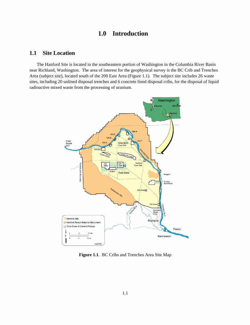
The Hanford Site is located in the southeastern portion of Washington in the Columbia River Basin near Richland, Washington. The area of interest for the geophysical survey is the BC Crib and Trenches Area (subject site), located south of the 200 East Area (Figure 1.1). The subject site includes 26 waste sites, including 20 unlined disposal trenches and 6 concrete lined disposal cribs, for the disposal of liquid radioactive mixed waste from the processing of uranium.
Figure 1.1. BC Cribs and Trenches Area Site Map
1.2
1.2 Objective of Investigation
The primary objective of this investigation was to characterize the subsurface of the subject site using several non-invasive geophysical methods. The characterization included identifying buried infra-structure from prior disposal activities and evaluating the extent of the radioactive contaminant plume known to exist from borehole data taken through the 216-B-26 Trench. The methods included total field magnetics, magnetic gradiometry, electromagnetic induction, and high resolution resistivity (HRR) and induced polarization (IP). Interpretations of the magnetic survey identified ferrous pipelines, suspected ferrous metallic debris, and probable basalt rocks used for drains. The electromagnetic data identified localized areas of conductive soil associated with liquid waste disposal, pipelines, suspected metallic debris (ferrous and non-ferrous), and areas in general where disposal and mitigation efforts have impacted the soil. The HRR survey provided information regarding an electrically conductive plume along transects around the subject site. The IP data provided no useful information regarding contaminant plume detection or migration.
1.3 Site Description
The BC Cribs and Trenches Area (also referred to as the BC Cribs and Trenches or BC Cribs) resides on the Central Plateau region of the Hanford Site. The site is located near the southwest corner of the 200 East Area and encompasses approximately 30 hectares of radiologically controlled land. Surface contamination areas are divided locally by radiologically released zones that facilitate access to well sampling vehicles that periodically enter the area.
The area that comprises the BC Cribs and Trenches is a part of two operable units and has been included in one study management area. These operable units and the management area are grouped according to media (groundwater or vadose), source facility, or by cleanup standard (Resource Conser-vation and Recovery Act [RCRA] or Comprehensive Environmental Response, Compensation, and Liability Act [CERCLA]). The BC Cribs and Trenches Area had been included in the 200-BP-2 Source Operable Unit. In 1993, the operable units near the 200 East Area were combined into two global operable units, 200-BP-5 (B Plant sources) and 200-PO-1 (Plutonium-Uranium Extraction [PUREX] Plant sources). These operable units, as well as the individual facilities comprising the BC Cribs and Trenches, are described in the B Plant Aggregate Area Management Area Report (DOE 1992). The latest grouping to which the BC Cribs and Trenches has been included is the 200-TW-1 Scavenged Waste Group Operable Unit. The name ‘BC Cribs’ also often confused with crib facilities in the 100-B/C Area.
In addition to carrying the identifier of 200-BP-2, the BC Cribs and Trenches have also been referred to as the BC Controlled Area (DOE 1992). This latter identifier refers to the BC Cribs and Trenches as well as an approximately 10.4-square-kilometer area of undisturbed, but surface contaminated, land that has been monitored as a radiologically controlled contamination area since May 1958. The source of the contamination is the animal feces from various local wildlife species that have either come in contact directly with salt precipitate at the BC Cribs and Trenches, or through ingestion of contaminated prey.
1.3
The BC Cribs and Trenches were constructed at various times throughout the 1950s. The BC Cribs and Trenches were stabilized in phases beginning with the trenches in 1969 and concluding in 1981 and 1982 with the addition of clean topsoil.
1.4 Operational History
Due to increased production demands and the consequent space limitations in the single-shell tanks, as well as the desire to recover unprocessed uranium, a scavenging process was begun in 1952 to simultaneously increase single-shell tank capacity and reduce T and B Plant waste volumes. Over the course of 6 years, wastes from Uranium Recovery Project and the ferrocyanide processes at the 221/224-U Plant were treated, the solids recovered, and the supernatant disposed of to the BC Cribs and Trenches. The waste has been referred to in several reports (DOE 1992, 2000) as scavenged waste. The 200-TW-1 Scavenged Waste Group Operable Unit, of which the BC Cribs and Trenches are a part, included the scavenged waste from 221-U Plant, as well as waste from the 300 Area Laboratory operations. The primary type of waste disposed in the BC Cribs and Trenches is liquid effluent from the 221/224-U Plant waste.
A ferrocyanide process was used to precipitate the soluble long-lived cesium-137 from the 221-U Building uranium recovery waste supernatant. These wastes had been stored in the B Tank Farms single-shell tanks. The insoluble strontium-90 was precipitated without adding chemicals. The precipi-tated waste was allowed to settle in single-shell tank storage and the solid precipitate particles settled to the bottom of the tanks as sludge. Following settling, the supernate was decanted from the sludge, tested for applicable discharge requirements, and discharged to the ground (DOE 1992).
A second campaign of scavenging began in May 1955 on 221-U Building tributyl phosphate waste that had also been stored in the single-shell tanks. The wastes were pumped to the 244-CR Vault near the PUREX Plant where they were scavenged. The waste was then routed back to single-shell tanks for settling, and supernatant subsequently was pumped to the ground. The “in-tank farm” scavenging in the 244-CR Vault ended in December 1957, with the last of these wastes being discharged to the ground in January 1958.
Waste management criteria for cribs and trenches required that several practical limits be considered before discharging supernatant liquids to the ground, but the most often cited in reports is the specific retention of the crib or trench. Specific retention refers to the volume of liquid that can be held under gravity by a defined soil volume. For the cribs and trenches, an estimate based on the unsaturated soil void space was calculated for each facility and that amount of liquid waste was discharged to the unit. Provided the unsaturated pore volume was correct, the liquid waste would be held high in the vadose and not reach groundwater. In the case of the BC Cribs and Trenches, the retention of waste from the scavenging operations appears to be accomplished by perching of the liquid fraction on a tightly-indurated clay layer with a possible pedogenic origin. 1.5 Geology
The geologic environment that underlies the BC Cribs and Trenches Area has been described in numerous reports including Tallman et al. (1979), the Consultation Draft Site Characterization Plan
1.4
(DOE 1988), Lindsey (1991), and Lindsey et al. (1994). Reports generated in support of the Integrated Disposal Facility (e.g., Reidel 2004) comprise the most comprehensive characterization data for a physical analog to the BC Cribs and Trenches. The sedimentary units described in Reidel (2004), to the depth covered in this report, include the sand-dominated facies of the Hanford formation, which has been locally divided into three layers. The layers are separated by paleosols that have not been correlated outside of the Integrated Disposal Facility, but appear to extend into the BC Cribs and Trenches Area.
Soil samples obtained in cone penetrometer borings (see Section 3.4) for this project (see Appendix A for photographic images of the cores) are Hanford formation sediments and exhibit medium- to fine-grained sediments that are interbedded coarse-grained, poorly sorted sand. The fine-grained sediments range from fine to very-fine sand. Cores from the first cone penetrometer advance both have a dense slit/clay layer resting on a coarser-grained sand layer. Cores from the second penetrometer have a less distinct layering and are generally massive medium-grained sands.

2.1
2.0 Theory
Magnetometry, electromagnetic induction, resistivity, and reduced polarization were all part of the investigation into subsurface contamination at the subject area. These concepts are outlined in the following sections to provide a context for discussing survey results and the conclusions derived from them.
2.1 Magnetometry
Magnetometry is the study of the earth’s magnetic field and is the oldest branch of geophysics (Telford et al. 1990). The earth’s field is composed of three main parts: the main field, which is internal, i.e., from a source within the earth that varies slowly in time and space; a secondary field, which is external to the earth and varies rapidly in time; and small internal fields constant in time and space, which are caused by local magnetic anomalies in the near-surface crust.
Of interest to the geophysicist are the localized anomalies. These anomalies are either caused by magnetic minerals (mainly magnetite or pyrrhotite) or buried steel and are the result of contrasts in the magnetic susceptibility (k). The average values for k are typically less than 1 for sedimentary formations and upwards to 20,000 for magnetite minerals.
The magnetic field is measured with a magnetometer. Magnetometers permit rapid, non-contact surveys to locate buried metallic objects and features. Portable (one person) field units can be used virtually anywhere that a person can walk, although they may be sensitive to local interferences, such as fences and overhead wires. Airborne magnetometers are towed by aircraft and are used to measure regional anomalies. Field-portable magnetometers may be single- or dual-sensor. Dual-sensor magnetometers are called gradiometers; they measure gradient of the magnetic field; single-sensor magnetometers measure total field.
Magnetic surveys are typically run with two separate magnetometers. The first magnetometer is used as a base station to record the earth’s primary field and the diurnally changing secondary field. The second magnetometer is used as a rover to measure the spatial variation of the earth’s field and may include various components (i.e., inclination, declination, and total intensity). By removing the temporal variation and, perhaps, the static value of the base station, from that of the rover, one is left with a residual magnetic field that is the result of local spatial variations only. The rover magnetometer is moved along a predetermined linear grid laid out at the site. Readings are virtually continuous and results can be monitored in the field as the survey proceeds.
The shortcoming with most magnetometers is that they only record the total magnetic field, F, and not the separate components of the vector field. This shortcoming can make the interpretation of magnetic anomalies difficult, especially since the strength of the field between the magnetometer and
2.2
target is reduced as a function of the inverse of distance cubed. Additional complications can include the inclination and declination of the earth’s field, the presence of any remnant magnetization associated with the target, and the shape of the target.
2.2 Electromagnetic Induction
Earth materials have the capacity to transmit electrical currents over a wide range and depend on the material property of electrical conductivity. Electrical conductivity is a function of soil type, porosity, saturation, and dissolved salts. Electromagnetic methods seek to identify various earth materials by measuring their electrical characteristics and interpreting results in terms of those characteristics.
Electromagnetic induction methods employ a transmitting coil (Tx) and a receiving coil (Rx) spaced at some given distance. Tx induces eddy currents in the earth, which themselves generate magnetic fields that are affected by the earth materials within the excited zone. Some parts of these fields are intercepted by Rx, resulting in an output voltage proportional to the terrain conductivity within the zone. By moving these coils laterally, variations in conductivity can be interpreted to find various buried features and/or objects. The Tx frequency and distance between Tx and Rx determine the depth of investigation, and the output permits construction of a stratigraphic profile of intervening depth.
2.3 Resistivity
The resistivity method is based on the capacity of earth materials to conduct electrical current. Earth resistivity is a function of soil type, porosity, moisture, and dissolved salts. The concept behind applying the resistivity method is to detect and map changes or distortions in an imposed electrical field due to heterogeneities in the subsurface.
Resistivity is a volumetric property measured in ohm-meters. Since it is not possible to know the exact volume or the mass of earth being measured under field conditions, readings are in terms of apparent resistivity.
The electric current may be generated by battery or motor-generator driven equipment depending on the particular application. Current is introduced into the ground through electrodes (metal rods). Earth-to-electrode coupling is typically enhanced by pouring water around the electrodes.
Field data are acquired using an electrode array. A four-electrode array employs an electric current injected into the earth through one pair of electrodes (transmitting dipole) and measures the resultant potential by the other pair (receiving dipole). The two most common configurations are Wenner and Schlumberger arrays. Their use depends upon site conditions and the information desired.
HRR methods generally employ a “pole-pole” array. For a pole-pole array, the two rover or “active” electrodes are incrementally spaced from 5 to 400 meters apart. The remaining two electrodes are placed at a distance greater than 800 meters from the rover electrodes, effectively rendering them at an “infinite” distance. The pole-pole array provides higher data density, increased signal to noise ratio, and requires less transmitted energy.
2.3
Data may be recorded manually or with a digital receiver. In either case, the data are reduced and processed using a PC and hydroGEOPHYSICS, Inc. (HGI) proprietary software. A rigorous quality control procedure is maintained to identify and either edit or delete questionable data points. The data are presented in color contoured cross sections of subsurface apparent resistivity using Golden Software’s Surfer software package (Version 8.02).
2.4 Induced Polarization
The equipment and set up for IP is identical to HRR. A pole-pole array is established and measure-ments are made in terms of an apparent polarization. However, IP differs by the way the measurements are made. In IP, the decay of voltage is measured over time. That is, as the direct current from the battery source is shut off, the voltage within the earth does not immediately return to zero. The voltage decays exponentially over a short time period (in milliseconds) and is the result of chemical energy storage due to variations in the mobility of ions in fluids in the subsurface and variations in ionic and electronic conduction where metallic minerals are present (Telford et al. 1990).
The most commonly used quantity for time-domain IP is chargeability (M). The chargeability is measured in millivolt-seconds per volt, or more simply, milliseconds and is the result of integrating the voltage decay between two time periods and normalizing to the static potential limit (potential at current shut-off).
Data may be recorded manually or with a digital receiver. In either case, the data are reduced and processed using a PC and HGI proprietary software. A rigorous quality control procedure is maintained to identify and either edit or delete questionable data points. The data are presented in color contoured cross sections of subsurface apparent resistivity using Golden Software’s Surfer software package (Version 8.02).
3.1
3.0 Methods
Many portions of the subject site are located within restricted zones with radioactive subsurface contamination. As a result, all field personnel were required to complete Radiation Worker Level II training and were provided dosimeters to monitor daily radiation doses. Additionally, upon exiting a soil contamination zone, personnel and equipment were surveyed for radiological contamination by a radiological technician. Personal protective equipment included steel-toed boots with cloth booties and gloves.
3.1 Survey Area and Logistics
To acquire data for the magnetic and electromagnetic surveys (Phase I), an all-terrain vehicle (ATV) was used to tow HGI’s Geophysical Operations Cart (G.O. Cart). The G.O. Cart was constructed of fiberglass, nylon, and plastic as to not interfere with the geophysical equipment. An extended tongue length of 4.6 meters was used to distance the ATV from the G.O. Cart. The G.O. Cart was equipped with two cesium-vapor magnetic sensors spaced 1 meter apart, a broadband electromagnetic sensor, and a differential global positioning system (GPS) for geo-referencing of geophysical data. All data was collected by a datalogger located on the ATV in front of the driver. The datalogger also allowed for the control of each instrument during data collection.
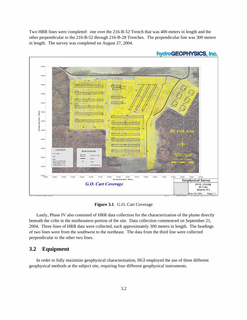
Data collection commenced on July 11, 2004, by establishing a magnetic base station (to remove diurnal variations of the magnetic field from the data collected on the G.O. Cart) and unpacking of the geophysical equipment. The G.O. Cart was operational on July 12, 2004, and data collection began over the cribs area. To collect the magnetic and electromagnetic data, the G.O. Cart was towed along parallel lines spaced approximately 2 to 3 meters apart. The speed of the ATV was controlled such that a nominal sampling rate of three measurements per meter was attained. G.O. Cart data collection formally finished on July 27, 2004, although several areas required additional coverage afterwards. Figure 3.1 shows the location of data points collected over the subject site.
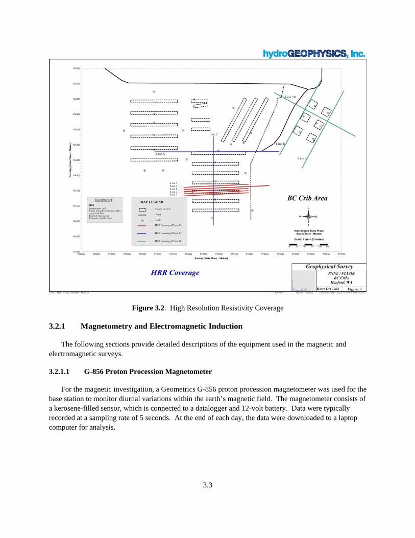
The Phase II HRR survey began on July 28, 2004. The HRR data were collected along five parallel east-west lines with line lengths of 200 to 300 meters. The lines were placed over the 216-B-26 Trench as well as 8 and 16 meters north and south of the trench. The lines extended approximately 33 meters off the ends of the trench to acquire background data. The exception was with the line 8 meters north of the center trench line, which was extended 133 meters off the east end of the trench (Figure 3.2). Phase II was completed on August 5, 2004.
In the initial proposal, it was suggested that Phase III consist of Residual Potential Mapping (RPM) to characterize the plume as a three-dimensional representation of contaminant migration. However, the Phase II HRR data revealed that the plume had spread sufficiently far to preclude the use of RPM. RPM requires a large amount of background data to statistically separate target from background. The plume extended beyond the limits of an RPM grid, thereby minimizing the amount of background data available. Therefore, it was decided to extend HRR coverage for Phase III, which began on August 25, 2004.
3.2
Two HRR lines were completed: one over the 216-B-52 Trench that was 400 meters in length and the other perpendicular to the 216-B-52 through 216-B-28 Trenches. The perpendicular line was 300 meters in length. The survey was completed on August 27, 2004.
Figure 3.1. G.O. Cart Coverage
Lastly, Phase IV also consisted of HRR data collection for the characterization of the plume directly beneath the cribs in the northeastern portion of the site. Data collection commenced on September 21, 2004. Three lines of HRR data were collected, each approximately 300 meters in length. The headings of two lines were from the southwest to the northeast. The data from the third line were collected perpendicular to the other two lines.
3.2 Equipment
In order to fully maximize geophysical characterization, HGI employed the use of three different geophysical methods at the subject site, requiring four different geophysical instruments.
3.3
Figure 3.2. High Resolution Resistivity Coverage
3.2.1 Magnetometry and Electromagnetic Induction
The following sections provide detailed descriptions of the equipment used in the magnetic and electromagnetic surveys.
3.2.1.1 G-856 Proton Procession Magnetometer
For the magnetic investigation, a Geometrics G-856 proton procession magnetometer was used for the base station to monitor diurnal variations within the earth’s magnetic field. The magnetometer consists of a kerosene-filled sensor, which is connected to a datalogger and 12-volt battery. Data were typically recorded at a sampling rate of 5 seconds. At the end of each day, the data were downloaded to a laptop computer for analysis.
3.4
3.2.1.2 G-858 Cesium Vapor Gradiometer
A Geometrics G-858 cesium vapor gradiometer was used to collect the total magnetic field and magnetic gradient data across the subject site. The G-858 was operated as a gradiometer (dual-sensor), with the sensors spaced vertically 1 meter apart with the lowest sensor being approximately 1 meter from the ground surface. In addition, the sensors were oriented vertically. A datalogger and control console was used to control the data collection, which was mounted in front of the driver of the ATV on the G.O. Cart. Data were recorded to an accuracy of 0.2 nanoTeslas (nT) in the range 20,000 to 120,000 nT at discrete time intervals. Time, date, and magnetic readings were stored in a datalogger and downloaded to a laptop PC for diurnal correction and processing.
Magnetic data were processed using specialized proprietary software, such as MAGMAPPER and Surfer. Data were de-spiked and corrected for diurnal effects, which can range up to 150 nT, and magnetic drift. A two-dimensional surface was finally derived that best fits long-wavelength components within the data. This crucial step (high-pass filtering) effectively removes the regional magnetic field and permits recognition of local anomalies. The resulting map clearly delineates magnetic anomalies; it may be compared with results of other geophysical methods (such as electromagnetic) to accurately locate specific subsurface objects and conditions.
3.2.1.3 GEM-2 Electromagnetic Conductivity and Susceptibility Instrument
Multi-frequency electromagnetic data were collected using a Geophex GEM-2 electromagnetic conductivity and susceptibility instrument. The GEM-2 consists of a sensor housing (ski) and electronics console. The ski was positioned broadside on the back of the G.O. Cart, i.e., the transmitter and receiving loops were orthogonal to direction of traverses. The loops are separated 1.66 meters apart and are horizontally placed on the G.O. Cart (i.e., vertical axis coils). The electronics console was connected directly to the G-858 console for datalogging capabilities. Both in-phase (real) and quadrature (imaginary) data were collected at five frequencies ranging from 5 kHz to 20 kHz. The electromagnetic data were then converted to electrical conductivity using the WinGEM software.
3.2.1.4 Trimble GPS
Geographic control for the magnetic and electromagnetic data was established using a Trimble AgGPS 132 navigation system. The GPS receiver was mounted approximately 1.5 meters above the G.O. Cart on a fiberglass rod. The GPS was connected directly to the G-858 console for datalogging capabilities. The sampling rate of the GPS was fixed at 1 reading/second. According to the manufacturer’s web site (www.trimble.com), the accuracy of the differential GPS is within 1 meter.
3.2.2 High Resolution Resistivity and Induced Polarization
The high resolution resistivity and induced polarization surveys both relied on one instrument to induce current and gather potential measurements. The following section describes the instrument in detail.
3.5
3.2.2.1 Advanced Geosciences Inc. Sting R8
HRR data were acquired using an Advanced Geosciences, Inc. (AGI) Super Sting R8 resistivity instrument in the pole-pole array configuration. The unit is a DC-powered, battery operated, low voltage, low amperage, automatic, eight channel resistivity and IP system. This system employs the SuperSting Swift general purpose cables that can be attached in series. Each cable segment contains four smart electrodes. Each electrode has the capability of acting as either a low-amperage current transmitter or as potential measuring receiver.
The Sting R-8 has the capability of automatically switching between electrodes without having to physically move the electrode connections after initial set-up. Automatic switching decreases physical labor, cuts down on human transcription and tracking errors, better allows the operator to control array logistics, and increases the rate and density of data acquired. HGI personnel took advantage of this capability and programmed the Sting R-8 to use a survey line spread of 72 smart electrodes with inter-electrode spacings ranging from 2 to 150 meters. The survey line was moved forward incrementally by removing a 12-electrode segment from the trailing end of the survey line spread and placing it at the front of the spread between measurements.
3.3 Data Processing
Each of the survey techniques requires preliminary data evaluation in the field followed by robust data processing and modeling at a computational facility. The final interpretation of the results is performed after the data processing and modeling is complete. In the following sections, an overview of that process is described.
3.3.1 Magnetometry
Data processing for the G-858 total-field magnetic data began with geo-referencing with respect to the differential GPS data. The GPS data were recorded at a sampling rate of 1 measurement/second, whereas the G-858 magnetic data were recorded at a rate of 5 measurements per second (an average of approximately 0.3 meter between measurements). Linear interpolation was used to geo-reference every magnetic data point. Spacing between successive lines of recorded data was approximately 2 meters. Additionally, the GPS indicated that data collection occurred at an elevation of 217 meters above mean sea level.
After geo-referencing, the G-858 magnetic data were corrected for diurnal variations in the earth’s magnetic field. The G-856 magnetic data were used for removing these variations by subtracting the base station data from the G-858 roving data. Before diurnal corrections, however, the G-856 base station data were de-spiked and filtered with a low-pass filter to remove high frequency noise.
The last step in time-series filtering of the G-858 magnetic data was to remove the heading error. Heading error results in the preferential alignment of the sensors in the earth’s magnetic field, which will cause anomalous readings unrelated to any response from buried metallic debris. Heading error was calculated from magnetic data collected in eight distinct directions. A curve was fit for direction of travel versus field strength, which was subsequently subtracted from the data.
3.6
The International Geomagnetic Reference Field (IGRF) was not subtracted from the magnetic data. The IGRF allows the removal of large-scale trends that could be present in magnetic data that covers large areas, and has a trend that is higher in the northern regions of the survey. The IGRF was calculated at the site using minimum and maximum longitude of 119.5443913 and 119.5443123 (approximately 500 meters) from the website http://www.ngdc.noaa.gov/seg/geomag/magfield.shtml. It was found that the IGRF varies by 2.2 nT and, therefore, was disregarded for this survey.
After correcting the G-858 magnetic data for each of the time-series issues, the data were compiled spatially and passed through a low-pass one-dimensional spatial filter to remove high frequency noise.
Additionally, coincident data points (within 0.03 meter) were removed to eliminate redundancy. Coincident data points were collected when the G.O. Cart was stationary while the instruments continued to collect data.
3.3.2 Electromagnetic Induction
The GEM-2 collects both in-phase and quadrature data of the electromagnetic signal. Typically, the in-phase is related to the magnetic susceptibility and the quadrature is related to the electrical conduc-tivity, each of which are a function of signal frequency, vertical distance of the coils to the ground, coil orientation (horizontal or vertical), and coil separation. For the GEM-2, the coil separation is fixed at 1.66 meters.
The first step in processing the electromagnetic data is geo-referencing of each data point with the differential GPS. The GPS data were recorded at a sampling rate of 1 measurement/second, whereas the GEM-2 electromagnetic data were recorded at a rate of 3 measurements per second. Linear interpolation was used to geo-reference every magnetic data point.
After geo-referencing, the in-phase and quadrature data were run through an inversion algorithm, provided to HGI by Geophex. The inversion algorithm converted the measured data to susceptibility and electrical conductivity. The results were susceptibility data for each of the five frequencies, electrical conductivity for each of the five frequencies, and a total electrical conductivity. The total electrical conductivity was calculated by equally weighting the individual frequencies in order to produce an average, frequency-independent electrical conductivity.
Once geo-referencing was complete, the data were shifted for the day-to-day changes in the data. The day-to-day changes were calculated from a coincident data collection run at the beginning of each collection day. Slight differences in the daily data records can be attributed to environmental or to instrument set-up changes. The first run of the day was collected along the entry road that ran perpendicular to the 216-B-26 to 216-B-58 Trenches.
After correcting the GEM-2 electromagnetic data for each of the time-series issues, the data were compiled spatially and passed through a low-pass one-dimensional spatial filter to remove high frequency noise. Additionally, coincident data points (within 0.03 meter) were removed to eliminate redundancy. Coincident data points were collected when the G.O. Cart was stationary while the instruments continued to collect data.
3.7
3.3.3 High Resolution Resistivity
HRR data are recorded digitally as apparent resistivity with the Sting R8 resistivity meter. The data are imported and filtered through HGIPro, a proprietary software application developed by HGI. Typically, apparent resistivity is presented as a pseudosection, where data points are plotted at depth at 45-degree intersections of the Tx and Rx. This linear plotting methodology is unrealistic and HGI has developed a geometrically-constrained inversion model to present the data more accurately. Additionally, the model allows for static corrections for topographical changes. After inversion, the data are checked for quality control.
3.3.4 Induced Polarization
IP data are recorded digitally for six decay waveform windows with the Sting R8 resistivity meter. The data are imported, summed, and filtered through HGIPro, a proprietary software developed by HGI. Typically, apparent chargeabilities are presented as a pseudosection, where data points are plotted at depth at 45-degree intersections of the Tx and Rx. This linear plotting methodology is unrealistic and HGI has developed a geometrically constrained inversion model to present the data more accurately. Additionally, the model allows for static corrections for topographical changes. After inversion, the data are checked for quality control.
3.4 Cone Penetrometer Sampling
To provide a context for interpreting the results obtained in the HRR surveys at the 216-B-26 Trench, two locations on Line 4 (Section 4.3.1.4) were selected for the purpose of gathering soil samples. The four samples obtained from cone penetrometer sampling were then submitted to the 325 Laboratory for analysis. The analytes selected reflected the best estimate of the parameters that would control conduc-tivity in the subsurface. The samples were analyzed for moisture, anions, and specific conductance. The samples were also analyzed for technetium-99 in order to evaluate the assumption that it would travel at the same rate and congregate in the same location as nitrate and the liquid fraction of the waste stream. Photographs of the liners submitted for analysis are in Appendix A.
Two samples were gathered at each of the two sampling locations. Prior to advancing the sampling penetrometer, a separate geophysical probe was pushed near the sampling location. The geophysical probe gathered information related to sleeve and tip pressure, soil conductivity, and soil moisture. After careful review of the geophysical probe data, it was determined that only the sleeve and tip pressure could be correlated to existing geophysical data. More work is planned for future borehole geophysics in an effort to obtain a resistivity model that will improve the correlation to surface geophysics results.
After gathering information related to sedimentary structure from the tip and sleeve pressure data, two sampling locations were selected. The results from the HRR work indicated that the plume depth varied from approximately 25 to 45 meters below ground surface. These target depths were initially selected for sampling with the cone penetrometer. It was later determined, however, that the rig and equipment used for this sampling exercise was not going to penetrate deeper than 27 meters. Two sampling points were
3.8
selected at points above 18 meters in depth, and two sample points were driven to their maximum depth before refusal (23 to 27 meters).
A total of five cone penetrometer advances were made the week of October 12, 2004. The first two cone penetrometer advances coincide with a point approximately 150 meters along Line 4 (Sec-tion 4.3.1.4). The objective for sampling in this location was to add to the data already developed in previous drilling exercises (e.g., well C4191), and to assess the concentration of contaminants in an area mapped with HRR as a low-conductivity zone. Well identifier C4673 was given to the geophysical probe penetration that advanced to 28.1 meters on October 12, 2004. The force required to move past this particular zone was deemed too great for the geophysical probe to sustain without shearing the drive pipe.
The sampling penetration (well C4674) began on the morning of October 13, 2004, and the first soil sample was obtained from a depth ranging from 10.1 to 10.8 meters. The sample was not immediately submitted to the laboratory. Although the sample was sealed, administrative problems at the drill site pushed the submission time into the afternoon of October 13. The second sample was captured the morning of October 14, 2004, from the depth range of 26.8 to 27.4 meters. This sample was immediately transported and submitted to the laboratory for analysis.
The second sampling location was originally identified as being approximately 80 meters along Line 4 (Section 4.3.1.4). The purpose of sampling in this location was to attempt to determine whether the maximum concentration of contaminants resided in those regions mapped with HRR as having the highest conductivity. Well identifier C4675 was given to the geophysical probe penetration advance on October 14, 2004. The cone penetrometer advance slowed approximately 3 hours into the push. The geophysical probe was withdrawn and the sampler was advanced with the objective of opening the borehole enough to advance past the fine-grained horizon which was the source of the refusal. Twenty minutes after the sampler cone penetrometer advance began, the pipe sheared near the surface leaving approximately 12.5 meters of pipe in the subsurface. Due to the loss of the soil sampler, and the refusal of the cone penetrometer at a relatively shallow depth, the cone penetrometer rig was moved to a position approximately 90 meters along Line 4.
The fourth boring was given the well identifier C4676. The geophysical penetration reached a depth of 18.9 meters on the morning of October 15, 2004. The difficulty in advancing beyond approximately 18.5 meters changed the sampling objectives of the second sampling location. The sampler would first advance to approximately 17 meters and take a sample just above the highest conductivity mapped with HRR. The next sample would be taken as deep in the boring as possible without endangering the sampler assembly. The second advance, given the identifier C4677, was begun with a “dummy” tip that would drive to refusal. This assembly would then be retracted and the sampler would be advanced to the sampling horizon. The third penetrometer sample was collected between 17 and 17.6 meters below grade. The sample was delivered to the laboratory by Fluor Hanford, Inc. radiation protection staff who then returned for the second sampling rung. The second dummy tip advance began in the late afternoon, reaching a depth of 21.6 meters. The sampling penetrometer was advanced to capture a sample in the horizon between 22.5 and 23.1 meters below grade. The sample was submitted to the laboratory on October 16, 2004.

4.1
4.0 Results and Interpretation
4.1 Magnetometry
The results of the magnetometry study indicate that metallic sources near the surface correlate with known or suspected abandoned piping and metallic deposits. The details are discussed in the following sections and provide data for the resistivity model used in high resolution resistivity analysis.
4.1.1 Total Magnetic Field
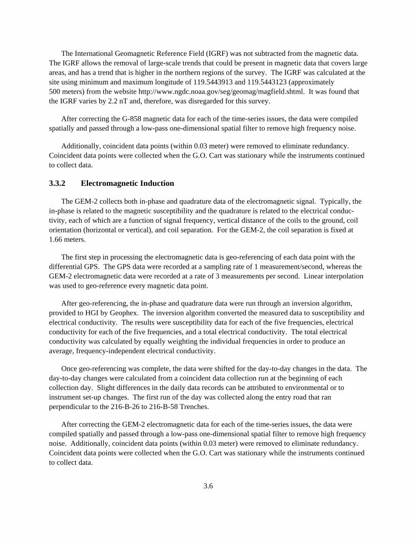
Figures 4.1 and 4.2 represent the results from the magnetic survey. Figure 4.1 is a color contour map of the residual total magnetic field, taken from the top sensor at 2 meters above ground. The data in Figure 4.1 have been processed and reduced according to the description in Section 3.3.1. The contour map was compiled from 375,726 data points kriged on a 2-meter-square grid. The semi-variogram used for the kriging algorithm was linear. Arithmetic averaging was used for multiple data points within the interpolated grid. The final data statistics indicate a minimum residual total magnetic field of -3,319 nT, a maximum of 9,312 nT, median of -129 nT, mean of -120 nT, and standard deviation of 175 nT (Table 4.1). Ambient total field intensity for the site is roughly 54,800 nT.
Figure 4.1 shows several pronounced monopolar and dipolar magnetic anomalies (colors red and blue) relative to the background (yellow). The yellow background color brackets the values from -200 to -40 nT and solid-line contours are at -220 and 60 nT. The anomalies are due to localized features and not to any large-scale geologic phenomena. The monopolar features show an extreme positive response in the total magnetic field and are a result of ferrous metallic objects at the lower sensor height that extend deeply into the subsurface. This correlates well with a few of the well casings that are approximately 1 meter above ground. For example, the well to the west of the 216-B-32 Trench shows a strong monopolar feature at a known well location. Another unknown monopolar feature exists directly east of the 216-B-28 Trench. Our interpretation of this response is that it represents the well that is, according to provided coordinates, located approximately 20 meters to the east (of the noted response). At the plotted well location, there is no monopolar magnetic response.
Figure 4.1 also shows several dipolar features. These dipolar features show a strong positive field to the south followed by a negative field to north. The dipolar features indicate limited vertical extent of a ferrous object. Additionally, there are linear anomalous features that would suggest ferrous metallic pipelines. Specifically, a pipeline network could possibly exist within the cribs area, located in the northeastern portion of the site. It appears that the pipeline arrives from the 200 East Area to the north of the site and forms a small distributed network of pipes that leads to the individual cribs. However, in addition to the total magnetic field anomaly from the pipeline within the crib area, distortions can be attributed to several monitoring wells in the area and possibly the use of basalt in the construction of the cribs.
4.2
Figure 4.1. Total Field Magnetics
Other possible pipeline networks can be seen within the 216-B-21, 216-B-33, and 216-B-34 Trenches. Interestingly, the pipeline network from the 216-B-33 and 216-B-34 Trenches appear to be connected at the eastern edge by a main pipeline coming from the 216-B-53A Trench. It is known from several aerial maps that a buried pipe exists approximately 25 meters to the west of the 216-B-53A Trench. The one other known pipeline that exists at the site is a gas pipe identified by signposts. The gas pipe is located northwest of the cribs area and to the east of the 216-B-20 Trench.
A few unknown anomalies exist around the site and are located at the 216-B-58 Trench and around the 216-B-52 Trench. The linear feature with the 216-B-58 Trench is not consistent with other pipelines around the site, but could possibly be due to perhaps something like discarded well casings. The response within the 216-B-52 Trench could be due to a pipeline but the signal is obstructed by a large amount of noise. These noisy features could be due to basalt cobbles that were observed during data collection on the G.O. Cart or signposts that were located around the site to designate soil contamination areas.
4.3
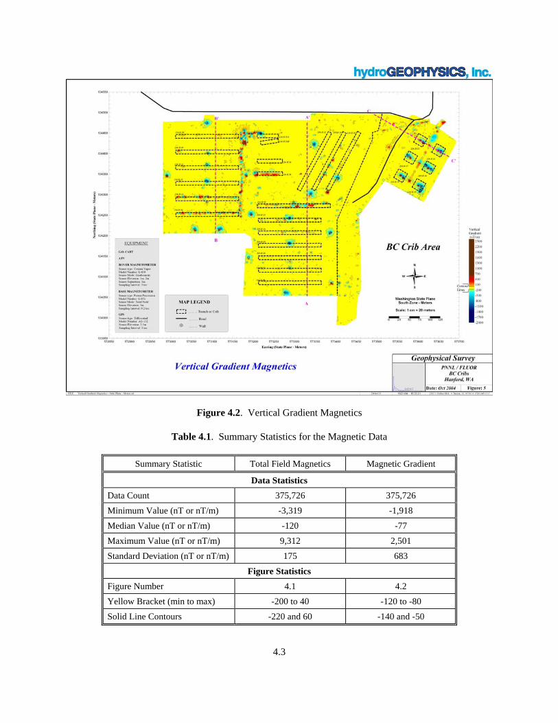
Figure 4.2. Vertical Gradient Magnetics
Table 4.1. Summary Statistics for the Magnetic Data
Summary Statistic Total Field Magnetics Magnetic Gradient
Data Statistics
Data Count 375,726 375,726
Minimum Value (nT or nT/m) -3,319 -1,918
Median Value (nT or nT/m) -120 -77
Maximum Value (nT or nT/m) 9,312 2,501
Standard Deviation (nT or nT/m) 175 683
Figure Statistics
Figure Number 4.1 4.2
Yellow Bracket (min to max) -200 to 40 -120 to -80
Solid Line Contours -220 and 60 -140 and -50
4.4
4.1.1.1 Magnetic Gradient
Figure 4.2 is a color contour map of the vertical magnetic gradient, which was calculated by sub-tracting the field of the lower sensor at 1 meter from the ground surface from the upper sensor located 2 meters above the ground surface. The contour map was compiled from 375,726 data points kriged on a 2-meter-square grid. The kriging semi-variogram was linear. Arithmetic averaging was used for multiple data points within the interpolated grid. The final data statistics are a minimum gradient of -1,918 nT/m, a maximum of 2,501 nT/m, median of -77 nT/m, mean of -85 nT/m, and standard deviation of 83 nT/m (Table 4.1).
Similar to Figure 4.1, Figure 4.2 has several pronounced monopolar and dipolar magnetic gradient anomalies (colors red and blue) relative to the background (yellow). The yellow background color brackets the values from -120 to -80 nT/m and solid line contours are at -140 and -50 nT/m. The anomalies are due to localized features and not to any large-scale geologic phenomena. The monopolar features show an extreme negative response in the magnetic gradient field, in particular around the monitoring wells. This is in contrast to many of the anomalies seen in the total magnetic field map of Figure 4.1, where many of the monitoring wells exhibited a dipolar response. The negative monopolar response in Figure 4.2 is a result of ferrous metallic objects (steel casing) being located at the height of the bottom sensor.
The dipolar features in Figure 4.2 are possibly a result of a distributed network of pipes. In particular, the pipelines within the cribs are more defined than that shown in the total magnetic field data because the interference of the monitoring wells have effectively been removed. The dipolar anomaly over the cribs show a distribution network of pipelines that arrive at the northern end of the area, with the possibility of a near-surface valve (monopolar response between the 216-B-14 and 216-B-15 Cribs) controlling the flow. The network distribution branches off to each of the cribs from the center line of the cribs.
Other pipeline responses can be seen in the 216-B-21, 216-B-33, and 216-B-34 Trenches. The anomalous responses in Figure 4.2 are very similar to that of Figure 4.1. The pipeline network from the 216-B-33 and 216-B-34 Trenches appears to be connected at the eastern edge by a main pipeline coming from the 216-B-53A Trench. It is known from several aerial maps that a buried pipe exists approximately 25 meters to the west of the 216-B-53A Trench. The one other known pipeline that exists at the site is a gas pipe identified by signposts. The gas pipe is located northwest of the cribs area and to the east of the 216-B-20 Trench.
A few unknown anomalies exist around the site and are located at the 216-B-58 Trench and around the 216-B-52 Trench. The linear feature with the 216-B-58 Trench is not consistent with other pipelines around the site, but could possibly be due to large metallic debris. The response within the 216-B-52 Trench could be due to a pipeline but the signal is obstructed by a large amount of noise. These noisy features could be due to basalt cobbles that were observed during data collection on the G.O. Cart or signposts that were located around the site to designate soil contamination areas.
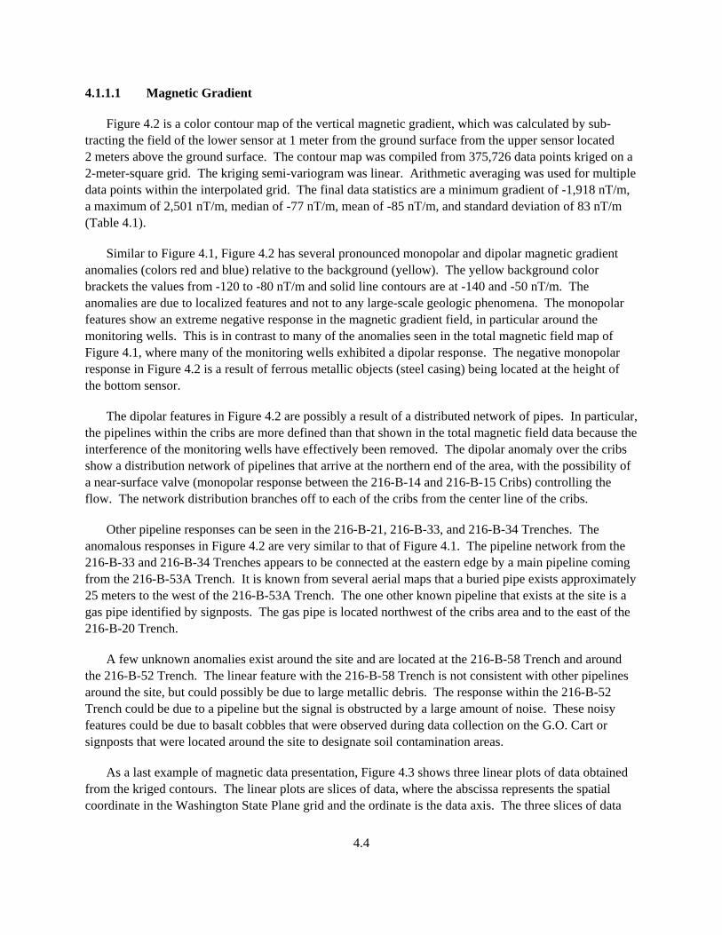
As a last example of magnetic data presentation, Figure 4.3 shows three linear plots of data obtained from the kriged contours. The linear plots are slices of data, where the abscissa represents the spatial coordinate in the Washington State Plane grid and the ordinate is the data axis. The three slices of data
4.5
shown in Figure 4.3 can be seen on the contour plots as purple dotted lines. Figure 4.3 also shows the relative locations of the trenches as depicted on the contour plots. Slice A-A’ through the center of the site confirms that the 216-B-22 and 216-B-23 Trenches, and 216-B-25 through 216-B-28 Trenches, do not have a significant magnetic signature. However, just north of the 216-B-25 Trench, a spike in the total magnetic field could be due to the basalt or cultural noise. The 216-B-24 and 216-B-52 Trenches show significant anomalies in the total magnetic field and to a lesser extent the vertical gradient. The broad positive anomaly in the total field at the northern end of slice A-A’ is due to the monitoring well.
Figure 4.3. Magnetic Data Slices Through BC Cribs
Slice B-B’ confirms the large features seen on the contour plots in the 216-B-33 and 216-B-34 Trenches. Again, these features are most likely due to a buried pipeline that was abandoned after the completion of the disposal activities. The largest anomaly in slice B-B’ is due to the monitoring well at the south end of the line.
The data within slice C-C’ overwhelmingly shows the effects of the monitoring wells with the 216-B-14 and 216-B-15 Cribs. The highest magnetic field values within the boundaries of the cribs correspond to the location of the wells. The other significant feature occurs between the cribs, where a pipeline is assumed to exist.
4.6
4.2 Electromagnetic Induction
The results of the electromagnetic induction studies exhibit patterns similar to those found in the magnetometry surveys described in Section 4.1. The information in this section provides additional modeling data for the high resolution resistivity surveys.
4.2.1 In-Phase Data
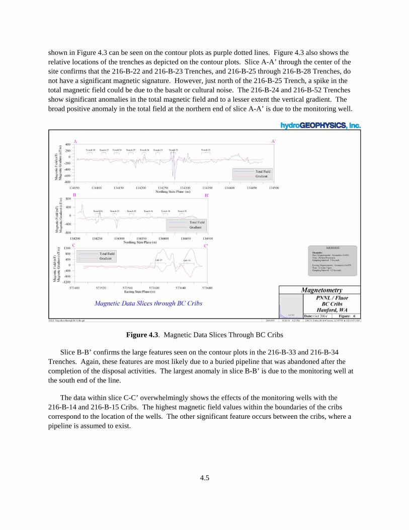
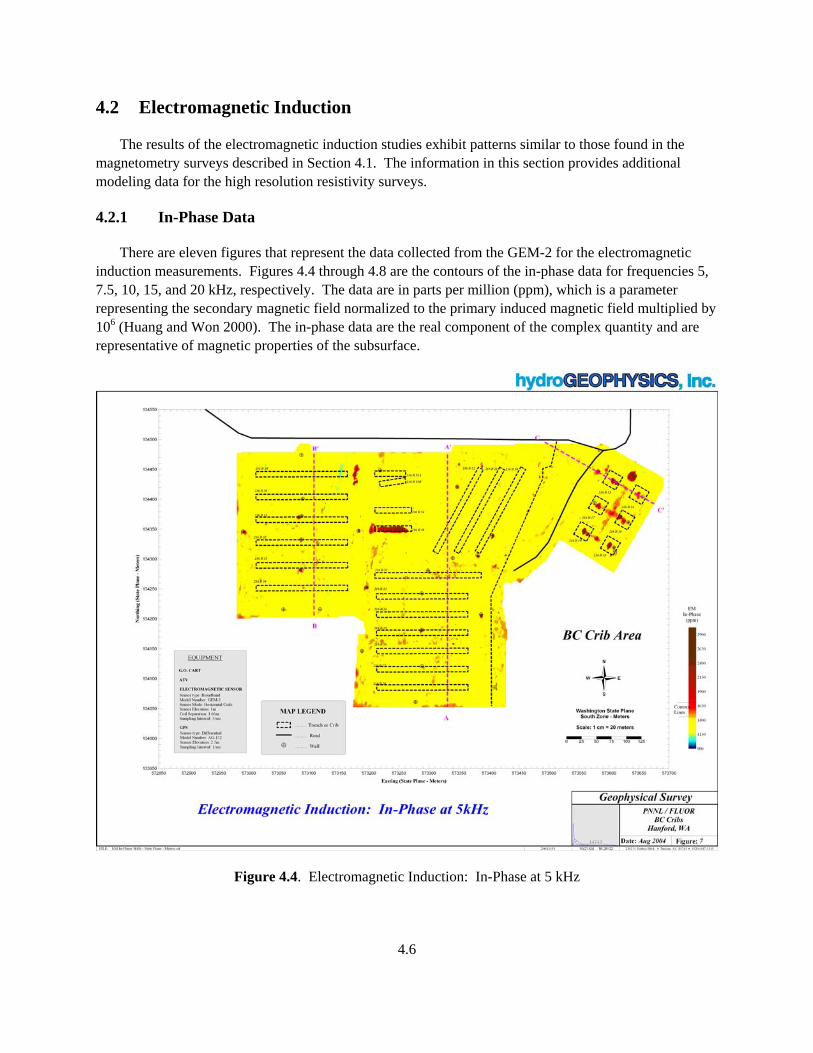
There are eleven figures that represent the data collected from the GEM-2 for the electromagnetic induction measurements. Figures 4.4 through 4.8 are the contours of the in-phase data for frequencies 5, 7.5, 10, 15, and 20 kHz, respectively. The data are in parts per million (ppm), which is a parameter representing the secondary magnetic field normalized to the primary induced magnetic field multiplied by 106 (Huang and Won 2000). The in-phase data are the real component of the complex quantity and are representative of magnetic properties of the subsurface.
Figure 4.4. Electromagnetic Induction: In-Phase at 5 kHz
4.7
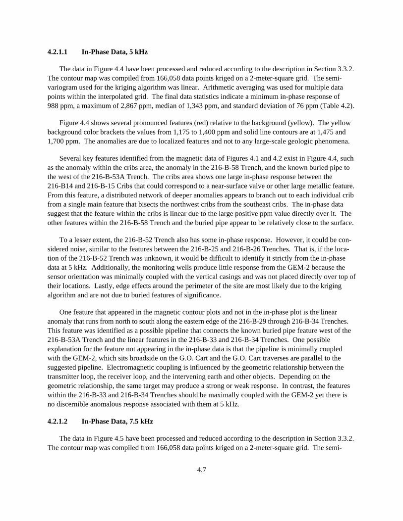
4.2.1.1 In-Phase Data, 5 kHz
The data in Figure 4.4 have been processed and reduced according to the description in Section 3.3.2. The contour map was compiled from 166,058 data points kriged on a 2-meter-square grid. The semi-variogram used for the kriging algorithm was linear. Arithmetic averaging was used for multiple data points within the interpolated grid. The final data statistics indicate a minimum in-phase response of 988 ppm, a maximum of 2,867 ppm, median of 1,343 ppm, and standard deviation of 76 ppm (Table 4.2).
Figure 4.4 shows several pronounced features (red) relative to the background (yellow). The yellow background color brackets the values from 1,175 to 1,400 ppm and solid line contours are at 1,475 and 1,700 ppm. The anomalies are due to localized features and not to any large-scale geologic phenomena.
Several key features identified from the magnetic data of Figures 4.1 and 4.2 exist in Figure 4.4, such as the anomaly within the cribs area, the anomaly in the 216-B-58 Trench, and the known buried pipe to the west of the 216-B-53A Trench. The cribs area shows one large in-phase response between the 216-B14 and 216-B-15 Cribs that could correspond to a near-surface valve or other large metallic feature. From this feature, a distributed network of deeper anomalies appears to branch out to each individual crib from a single main feature that bisects the northwest cribs from the southeast cribs. The in-phase data suggest that the feature within the cribs is linear due to the large positive ppm value directly over it. The other features within the 216-B-58 Trench and the buried pipe appear to be relatively close to the surface.
To a lesser extent, the 216-B-52 Trench also has some in-phase response. However, it could be con-sidered noise, similar to the features between the 216-B-25 and 216-B-26 Trenches. That is, if the loca-tion of the 216-B-52 Trench was unknown, it would be difficult to identify it strictly from the in-phase data at 5 kHz. Additionally, the monitoring wells produce little response from the GEM-2 because the sensor orientation was minimally coupled with the vertical casings and was not placed directly over top of their locations. Lastly, edge effects around the perimeter of the site are most likely due to the kriging algorithm and are not due to buried features of significance.
One feature that appeared in the magnetic contour plots and not in the in-phase plot is the linear anomaly that runs from north to south along the eastern edge of the 216-B-29 through 216-B-34 Trenches. This feature was identified as a possible pipeline that connects the known buried pipe feature west of the 216-B-53A Trench and the linear features in the 216-B-33 and 216-B-34 Trenches. One possible explanation for the feature not appearing in the in-phase data is that the pipeline is minimally coupled with the GEM-2, which sits broadside on the G.O. Cart and the G.O. Cart traverses are parallel to the suggested pipeline. Electromagnetic coupling is influenced by the geometric relationship between the transmitter loop, the receiver loop, and the intervening earth and other objects. Depending on the geometric relationship, the same target may produce a strong or weak response. In contrast, the features within the 216-B-33 and 216-B-34 Trenches should be maximally coupled with the GEM-2 yet there is no discernible anomalous response associated with them at 5 kHz.
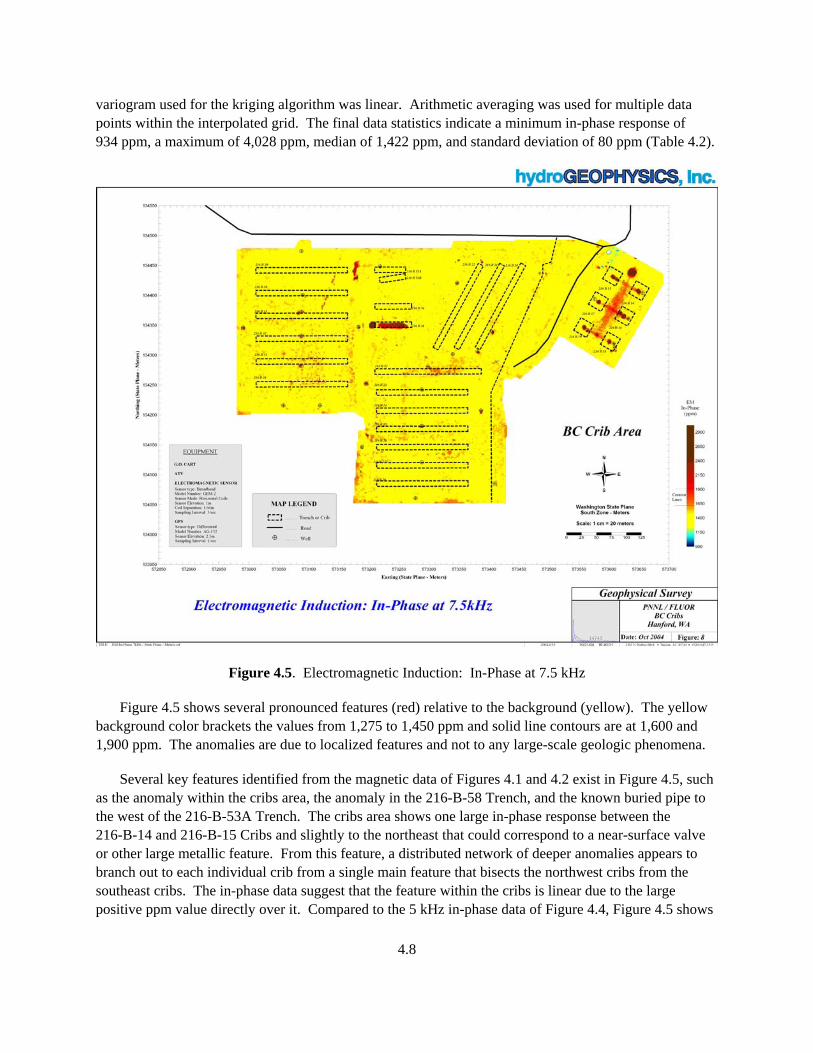
4.2.1.2 In-Phase Data, 7.5 kHz
The data in Figure 4.5 have been processed and reduced according to the description in Section 3.3.2. The contour map was compiled from 166,058 data points kriged on a 2-meter-square grid. The semi-
4.8
variogram used for the kriging algorithm was linear. Arithmetic averaging was used for multiple data points within the interpolated grid. The final data statistics indicate a minimum in-phase response of 934 ppm, a maximum of 4,028 ppm, median of 1,422 ppm, and standard deviation of 80 ppm (Table 4.2).
Figure 4.5. Electromagnetic Induction: In-Phase at 7.5 kHz
Figure 4.5 shows several pronounced features (red) relative to the background (yellow). The yellow background color brackets the values from 1,275 to 1,450 ppm and solid line contours are at 1,600 and 1,900 ppm. The anomalies are due to localized features and not to any large-scale geologic phenomena.
Several key features identified from the magnetic data of Figures 4.1 and 4.2 exist in Figure 4.5, such as the anomaly within the cribs area, the anomaly in the 216-B-58 Trench, and the known buried pipe to the west of the 216-B-53A Trench. The cribs area shows one large in-phase response between the 216-B-14 and 216-B-15 Cribs and slightly to the northeast that could correspond to a near-surface valve or other large metallic feature. From this feature, a distributed network of deeper anomalies appears to branch out to each individual crib from a single main feature that bisects the northwest cribs from the southeast cribs. The in-phase data suggest that the feature within the cribs is linear due to the large positive ppm value directly over it. Compared to the 5 kHz in-phase data of Figure 4.4, Figure 4.5 shows
4.9
a larger response. The other features within the 216-B-58 Trench and the buried pipe appear to be relatively close to the surface.
To a lesser extent, the 216-B-52, 216-B-33, and 216-B-34 Trenches also have some generally asso-ciated in-phase response. However, these data could be considered noise, similar to the features between the 216-B-25 and 216-B-26 Trenches. That is, if the location of these trenches were unknown, it would be difficult to identify them strictly from the in-phase data at 7.5 kHz. Additionally, the monitoring wells produce little response from the GEM-2 because of minimal coupling. Lastly, edge effects around the perimeter of the site are most likely due to the kriging algorithm and are not due to buried features of significance.
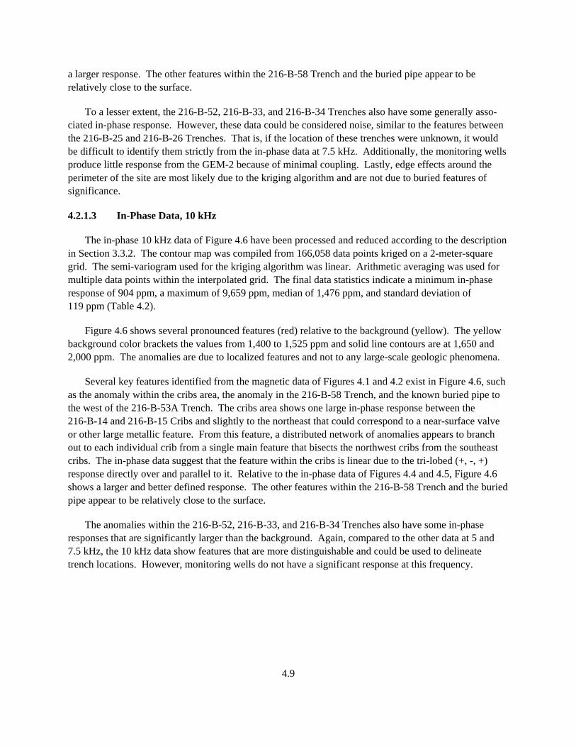
4.2.1.3 In-Phase Data, 10 kHz
The in-phase 10 kHz data of Figure 4.6 have been processed and reduced according to the description in Section 3.3.2. The contour map was compiled from 166,058 data points kriged on a 2-meter-square grid. The semi-variogram used for the kriging algorithm was linear. Arithmetic averaging was used for multiple data points within the interpolated grid. The final data statistics indicate a minimum in-phase response of 904 ppm, a maximum of 9,659 ppm, median of 1,476 ppm, and standard deviation of 119 ppm (Table 4.2).
Figure 4.6 shows several pronounced features (red) relative to the background (yellow). The yellow background color brackets the values from 1,400 to 1,525 ppm and solid line contours are at 1,650 and 2,000 ppm. The anomalies are due to localized features and not to any large-scale geologic phenomena.
Several key features identified from the magnetic data of Figures 4.1 and 4.2 exist in Figure 4.6, such as the anomaly within the cribs area, the anomaly in the 216-B-58 Trench, and the known buried pipe to the west of the 216-B-53A Trench. The cribs area shows one large in-phase response between the 216-B-14 and 216-B-15 Cribs and slightly to the northeast that could correspond to a near-surface valve or other large metallic feature. From this feature, a distributed network of anomalies appears to branch out to each individual crib from a single main feature that bisects the northwest cribs from the southeast cribs. The in-phase data suggest that the feature within the cribs is linear due to the tri-lobed (+, -, +) response directly over and parallel to it. Relative to the in-phase data of Figures 4.4 and 4.5, Figure 4.6 shows a larger and better defined response. The other features within the 216-B-58 Trench and the buried pipe appear to be relatively close to the surface.
The anomalies within the 216-B-52, 216-B-33, and 216-B-34 Trenches also have some in-phase responses that are significantly larger than the background. Again, compared to the other data at 5 and 7.5 kHz, the 10 kHz data show features that are more distinguishable and could be used to delineate trench locations. However, monitoring wells do not have a significant response at this frequency.
4.10
Figure 4.6. Electromagnetic Induction: In-Phase at 10 kHz
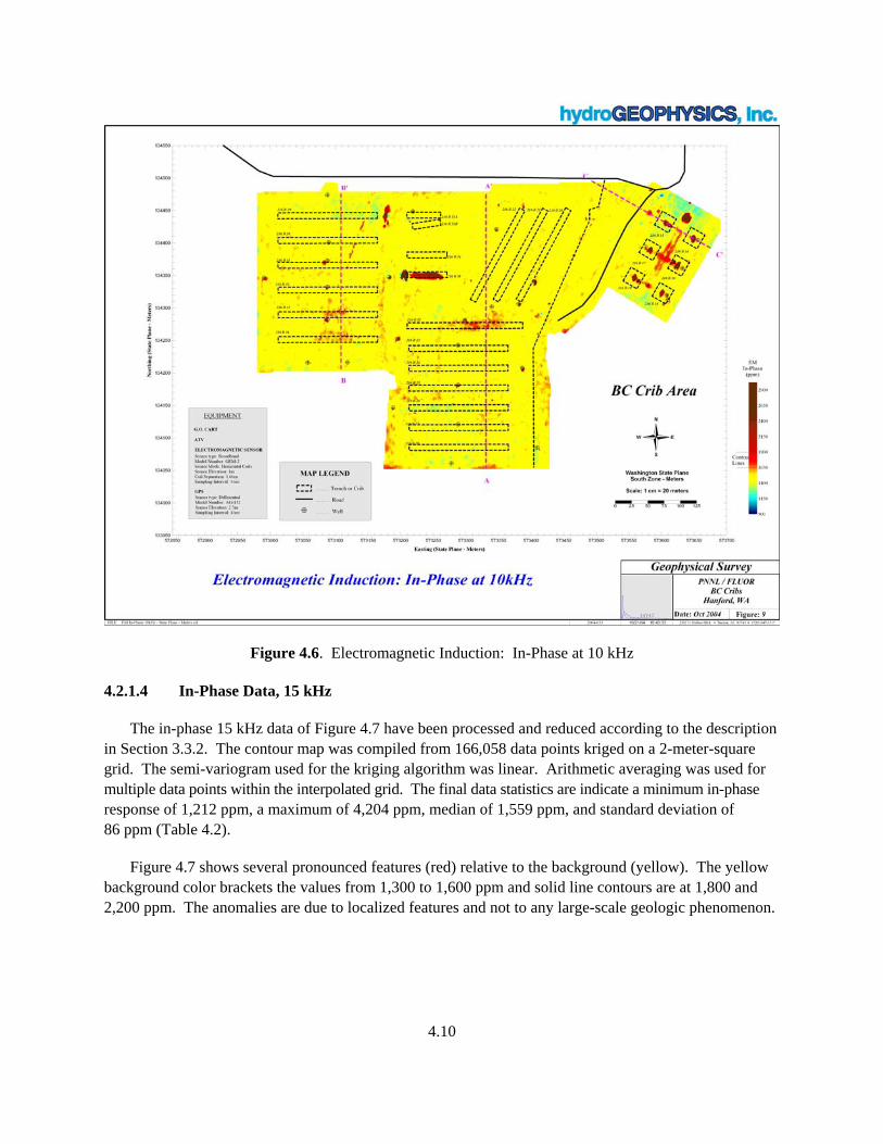
4.2.1.4 In-Phase Data, 15 kHz
The in-phase 15 kHz data of Figure 4.7 have been processed and reduced according to the description in Section 3.3.2. The contour map was compiled from 166,058 data points kriged on a 2-meter-square grid. The semi-variogram used for the kriging algorithm was linear. Arithmetic averaging was used for multiple data points within the interpolated grid. The final data statistics are indicate a minimum in-phase response of 1,212 ppm, a maximum of 4,204 ppm, median of 1,559 ppm, and standard deviation of 86 ppm (Table 4.2).
Figure 4.7 shows several pronounced features (red) relative to the background (yellow). The yellow background color brackets the values from 1,300 to 1,600 ppm and solid line contours are at 1,800 and 2,200 ppm. The anomalies are due to localized features and not to any large-scale geologic phenomenon.
4.11
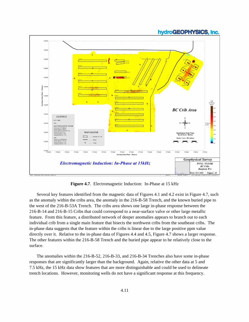
Figure 4.7. Electromagnetic Induction: In-Phase at 15 kHz
Several key features identified from the magnetic data of Figures 4.1 and 4.2 exist in Figure 4.7, such as the anomaly within the cribs area, the anomaly in the 216-B-58 Trench, and the known buried pipe to the west of the 216-B-53A Trench. The cribs area shows one large in-phase response between the 216-B-14 and 216-B-15 Cribs that could correspond to a near-surface valve or other large metallic feature. From this feature, a distributed network of deeper anomalies appears to branch out to each individual crib from a single main feature that bisects the northwest cribs from the southeast cribs. The in-phase data suggests that the feature within the cribs is linear due to the large positive ppm value directly over it. Relative to the in-phase data of Figures 4.4 and 4.5, Figure 4.7 shows a larger response. The other features within the 216-B-58 Trench and the buried pipe appear to be relatively close to the surface.
The anomalies within the 216-B-52, 216-B-33, and 216-B-34 Trenches also have some in-phase responses that are significantly larger than the background. Again, relative the other data at 5 and 7.5 kHz, the 15 kHz data show features that are more distinguishable and could be used to delineate trench locations. However, monitoring wells do not have a significant response at this frequency.
4.12
4.2.1.5 In-Phase Data, 20 kHz
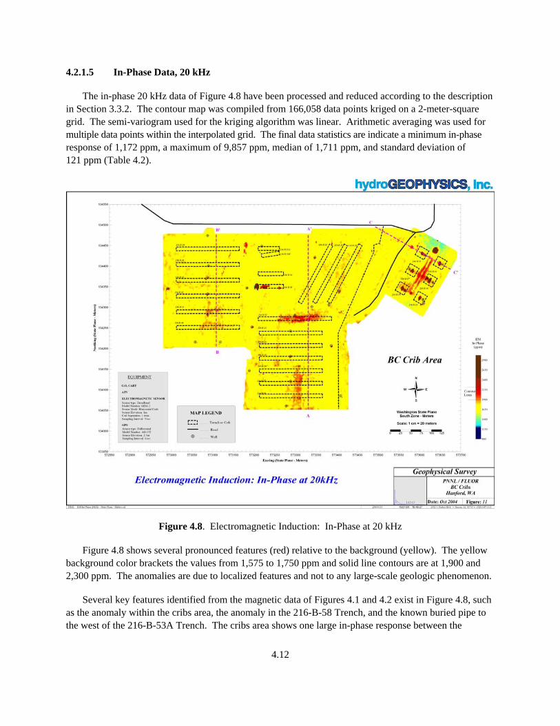
The in-phase 20 kHz data of Figure 4.8 have been processed and reduced according to the description in Section 3.3.2. The contour map was compiled from 166,058 data points kriged on a 2-meter-square grid. The semi-variogram used for the kriging algorithm was linear. Arithmetic averaging was used for multiple data points within the interpolated grid. The final data statistics are indicate a minimum in-phase response of 1,172 ppm, a maximum of 9,857 ppm, median of 1,711 ppm, and standard deviation of 121 ppm (Table 4.2).
Figure 4.8. Electromagnetic Induction: In-Phase at 20 kHz
Figure 4.8 shows several pronounced features (red) relative to the background (yellow). The yellow background color brackets the values from 1,575 to 1,750 ppm and solid line contours are at 1,900 and 2,300 ppm. The anomalies are due to localized features and not to any large-scale geologic phenomenon.
Several key features identified from the magnetic data of Figures 4.1 and 4.2 exist in Figure 4.8, such as the anomaly within the cribs area, the anomaly in the 216-B-58 Trench, and the known buried pipe to the west of the 216-B-53A Trench. The cribs area shows one large in-phase response between the
4.13
216-B-14 and 216-B-15 Cribs that could correspond to a near-surface valve or other large metallic feature. From this feature, a distributed network of deeper anomalies appears to branch out to each individual crib from a single main feature that bisects the northwest cribs from the southeast cribs. The in-phase data suggests that the feature within the cribs is linear due to the large positive ppm value directly over it. Relative to the in-phase data of Figures 4.4 and 4.5, Figure 4.8 shows a larger response. The other features within the 216-B-58 Trench and the buried pipe appear to be relatively close to the surface.
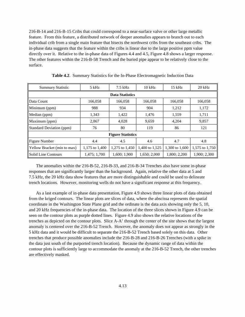
Table 4.2. Summary Statistics for the In-Phase Electromagnetic Induction Data
Summary Statistic 5 kHz 7.5 kHz 10 kHz 15 kHz 20 kHz
Data Statistics
Data Count 166,058 166,058 166,058 166,058 166,058
Minimum (ppm) 988 934 904 1,212 1,172
Median (ppm) 1,343 1,422 1,476 1,559 1,711
Maximum (ppm) 2,867 4,028 9,659 4,204 9,857
Standard Deviation (ppm) 76 80 119 86 121
Figure Statistics
Figure Number 4.4 4.5 4.6 4.7 4.8
Yellow Bracket (min to max) 1,175 to 1,400 1,275 to 1,450 1,400 to 1,525 1,300 to 1,600 1,575 to 1,750
Solid Line Contours 1,475; 1,700 1,600; 1,900 1,650; 2,000 1,800; 2,200 1,900; 2,300
The anomalies within the 216-B-52, 216-B-33, and 216-B-34 Trenches also have some in-phase responses that are significantly larger than the background. Again, relative the other data at 5 and 7.5 kHz, the 20 kHz data show features that are more distinguishable and could be used to delineate trench locations. However, monitoring wells do not have a significant response at this frequency.
As a last example of in-phase data presentation, Figure 4.9 shows three linear plots of data obtained from the kriged contours. The linear plots are slices of data, where the abscissa represents the spatial coordinate in the Washington State Plane grid and the ordinate is the data axis showing only the 5, 10, and 20 kHz frequencies of the in-phase data. The location of the three slices shown in Figure 4.9 can be seen on the contour plots as purple dotted lines. Figure 4.9 also shows the relative locations of the trenches as depicted on the contour plots. Slice A-A’ through the center of the site shows that the largest anomaly is centered over the 216-B-52 Trench. However, the anomaly does not appear as strongly in the 5 kHz data and it would be difficult to separate the 216-B-52 Trench based solely on this data. Other trenches that produce possible anomalies include the 216-B-28 and 216-B-26 Trenches (with a spike in the data just south of the purported trench location). Because the dynamic range of data within the contour plots is sufficiently large to accommodate the anomaly at the 216-B-52 Trench, the other trenches are effectively masked.
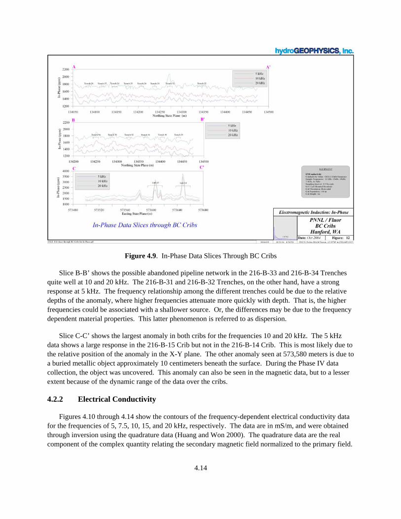
4.14
Figure 4.9. In-Phase Data Slices Through BC Cribs
Slice B-B’ shows the possible abandoned pipeline network in the 216-B-33 and 216-B-34 Trenches quite well at 10 and 20 kHz. The 216-B-31 and 216-B-32 Trenches, on the other hand, have a strong response at 5 kHz. The frequency relationship among the different trenches could be due to the relative depths of the anomaly, where higher frequencies attenuate more quickly with depth. That is, the higher frequencies could be associated with a shallower source. Or, the differences may be due to the frequency dependent material properties. This latter phenomenon is referred to as dispersion.
Slice C-C’ shows the largest anomaly in both cribs for the frequencies 10 and 20 kHz. The 5 kHz data shows a large response in the 216-B-15 Crib but not in the 216-B-14 Crib. This is most likely due to the relative position of the anomaly in the X-Y plane. The other anomaly seen at 573,580 meters is due to a buried metallic object approximately 10 centimeters beneath the surface. During the Phase IV data collection, the object was uncovered. This anomaly can also be seen in the magnetic data, but to a lesser extent because of the dynamic range of the data over the cribs.
4.2.2 Electrical Conductivity
Figures 4.10 through 4.14 show the contours of the frequency-dependent electrical conductivity data for the frequencies of 5, 7.5, 10, 15, and 20 kHz, respectively. The data are in mS/m, and were obtained through inversion using the quadrature data (Huang and Won 2000). The quadrature data are the real component of the complex quantity relating the secondary magnetic field normalized to the primary field.
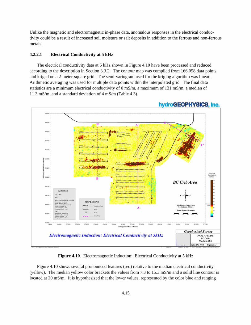
4.15
Unlike the magnetic and electromagnetic in-phase data, anomalous responses in the electrical conduc-tivity could be a result of increased soil moisture or salt deposits in addition to the ferrous and non-ferrous metals.
4.2.2.1 Electrical Conductivity at 5 kHz
The electrical conductivity data at 5 kHz shown in Figure 4.10 have been processed and reduced according to the description in Section 3.3.2. The contour map was compiled from 166,058 data points and kriged on a 2-meter-square grid. The semi-variogram used for the kriging algorithm was linear. Arithmetic averaging was used for multiple data points within the interpolated grid. The final data statistics are a minimum electrical conductivity of 0 mS/m, a maximum of 131 mS/m, a median of 11.3 mS/m, and a standard deviation of 4 mS/m (Table 4.3).
Figure 4.10. Electromagnetic Induction: Electrical Conductivity at 5 kHz
Figure 4.10 shows several pronounced features (red) relative to the median electrical conductivity (yellow). The median yellow color brackets the values from 7.3 to 15.3 mS/m and a solid line contour is located at 20 mS/m. It is hypothesized that the lower values, represented by the color blue and ranging
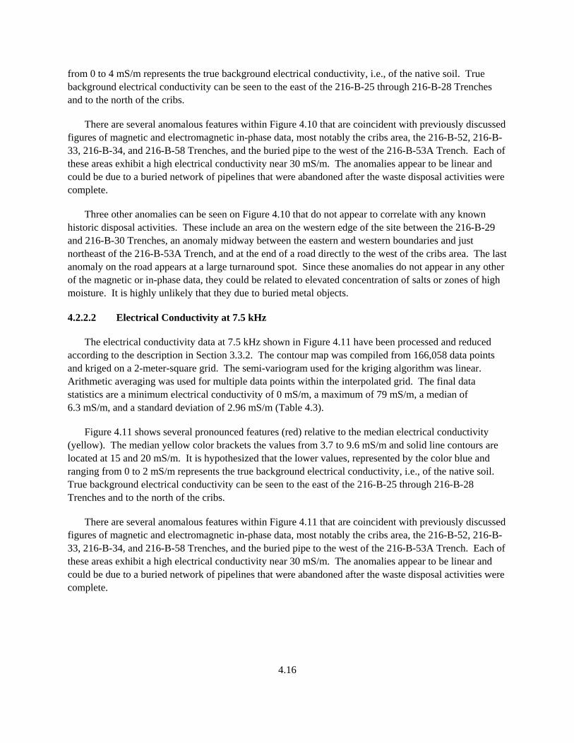
4.16
from 0 to 4 mS/m represents the true background electrical conductivity, i.e., of the native soil. True background electrical conductivity can be seen to the east of the 216-B-25 through 216-B-28 Trenches and to the north of the cribs.
There are several anomalous features within Figure 4.10 that are coincident with previously discussed figures of magnetic and electromagnetic in-phase data, most notably the cribs area, the 216-B-52, 216-B-33, 216-B-34, and 216-B-58 Trenches, and the buried pipe to the west of the 216-B-53A Trench. Each of these areas exhibit a high electrical conductivity near 30 mS/m. The anomalies appear to be linear and could be due to a buried network of pipelines that were abandoned after the waste disposal activities were complete.
Three other anomalies can be seen on Figure 4.10 that do not appear to correlate with any known historic disposal activities. These include an area on the western edge of the site between the 216-B-29 and 216-B-30 Trenches, an anomaly midway between the eastern and western boundaries and just northeast of the 216-B-53A Trench, and at the end of a road directly to the west of the cribs area. The last anomaly on the road appears at a large turnaround spot. Since these anomalies do not appear in any other of the magnetic or in-phase data, they could be related to elevated concentration of salts or zones of high moisture. It is highly unlikely that they due to buried metal objects.
4.2.2.2 Electrical Conductivity at 7.5 kHz
The electrical conductivity data at 7.5 kHz shown in Figure 4.11 have been processed and reduced according to the description in Section 3.3.2. The contour map was compiled from 166,058 data points and kriged on a 2-meter-square grid. The semi-variogram used for the kriging algorithm was linear. Arithmetic averaging was used for multiple data points within the interpolated grid. The final data statistics are a minimum electrical conductivity of 0 mS/m, a maximum of 79 mS/m, a median of 6.3 mS/m, and a standard deviation of 2.96 mS/m (Table 4.3).
Figure 4.11 shows several pronounced features (red) relative to the median electrical conductivity (yellow). The median yellow color brackets the values from 3.7 to 9.6 mS/m and solid line contours are located at 15 and 20 mS/m. It is hypothesized that the lower values, represented by the color blue and ranging from 0 to 2 mS/m represents the true background electrical conductivity, i.e., of the native soil. True background electrical conductivity can be seen to the east of the 216-B-25 through 216-B-28 Trenches and to the north of the cribs.
There are several anomalous features within Figure 4.11 that are coincident with previously discussed figures of magnetic and electromagnetic in-phase data, most notably the cribs area, the 216-B-52, 216-B-33, 216-B-34, and 216-B-58 Trenches, and the buried pipe to the west of the 216-B-53A Trench. Each of these areas exhibit a high electrical conductivity near 30 mS/m. The anomalies appear to be linear and could be due to a buried network of pipelines that were abandoned after the waste disposal activities were complete.
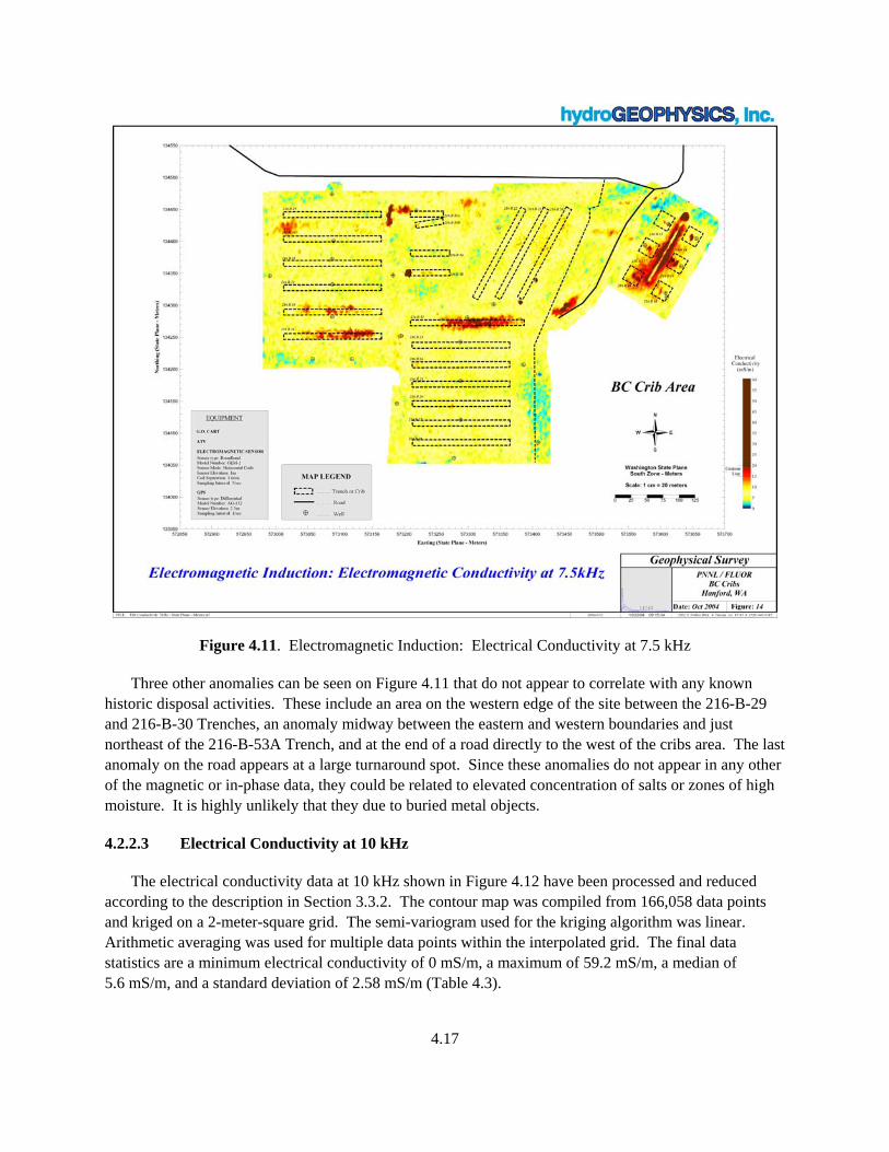
4.17
Figure 4.11. Electromagnetic Induction: Electrical Conductivity at 7.5 kHz
Three other anomalies can be seen on Figure 4.11 that do not appear to correlate with any known historic disposal activities. These include an area on the western edge of the site between the 216-B-29 and 216-B-30 Trenches, an anomaly midway between the eastern and western boundaries and just northeast of the 216-B-53A Trench, and at the end of a road directly to the west of the cribs area. The last anomaly on the road appears at a large turnaround spot. Since these anomalies do not appear in any other of the magnetic or in-phase data, they could be related to elevated concentration of salts or zones of high moisture. It is highly unlikely that they due to buried metal objects.
4.2.2.3 Electrical Conductivity at 10 kHz
The electrical conductivity data at 10 kHz shown in Figure 4.12 have been processed and reduced according to the description in Section 3.3.2. The contour map was compiled from 166,058 data points and kriged on a 2-meter-square grid. The semi-variogram used for the kriging algorithm was linear. Arithmetic averaging was used for multiple data points within the interpolated grid. The final data statistics are a minimum electrical conductivity of 0 mS/m, a maximum of 59.2 mS/m, a median of 5.6 mS/m, and a standard deviation of 2.58 mS/m (Table 4.3).
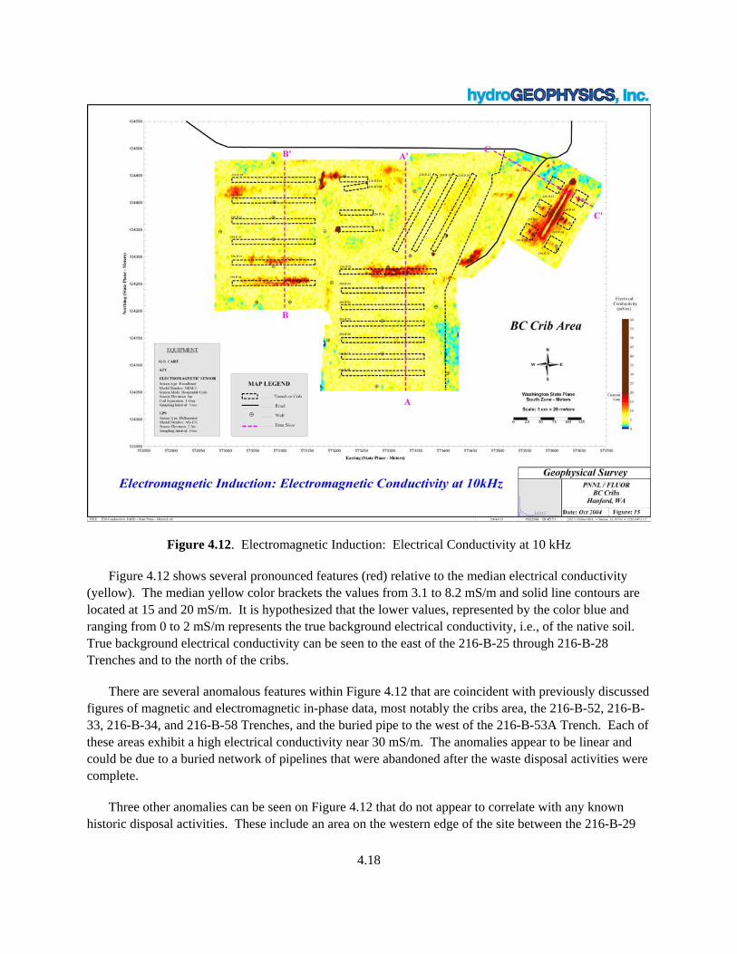
4.18
Figure 4.12. Electromagnetic Induction: Electrical Conductivity at 10 kHz
Figure 4.12 shows several pronounced features (red) relative to the median electrical conductivity (yellow). The median yellow color brackets the values from 3.1 to 8.2 mS/m and solid line contours are located at 15 and 20 mS/m. It is hypothesized that the lower values, represented by the color blue and ranging from 0 to 2 mS/m represents the true background electrical conductivity, i.e., of the native soil. True background electrical conductivity can be seen to the east of the 216-B-25 through 216-B-28 Trenches and to the north of the cribs.
There are several anomalous features within Figure 4.12 that are coincident with previously discussed figures of magnetic and electromagnetic in-phase data, most notably the cribs area, the 216-B-52, 216-B-33, 216-B-34, and 216-B-58 Trenches, and the buried pipe to the west of the 216-B-53A Trench. Each of these areas exhibit a high electrical conductivity near 30 mS/m. The anomalies appear to be linear and could be due to a buried network of pipelines that were abandoned after the waste disposal activities were complete.
Three other anomalies can be seen on Figure 4.12 that do not appear to correlate with any known historic disposal activities. These include an area on the western edge of the site between the 216-B-29
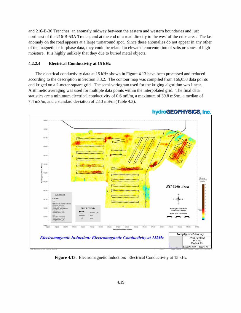
4.19
and 216-B-30 Trenches, an anomaly midway between the eastern and western boundaries and just northeast of the 216-B-53A Trench, and at the end of a road directly to the west of the cribs area. The last anomaly on the road appears at a large turnaround spot. Since these anomalies do not appear in any other of the magnetic or in-phase data, they could be related to elevated concentration of salts or zones of high moisture. It is highly unlikely that they due to buried metal objects.
4.2.2.4 Electrical Conductivity at 15 kHz
The electrical conductivity data at 15 kHz shown in Figure 4.13 have been processed and reduced according to the description in Section 3.3.2. The contour map was compiled from 166,058 data points and kriged on a 2-meter-square grid. The semi-variogram used for the kriging algorithm was linear. Arithmetic averaging was used for multiple data points within the interpolated grid. The final data statistics are a minimum electrical conductivity of 0.6 mS/m, a maximum of 39.8 mS/m, a median of 7.4 mS/m, and a standard deviation of 2.13 mS/m (Table 4.3).
Figure 4.13. Electromagnetic Induction: Electrical Conductivity at 15 kHz
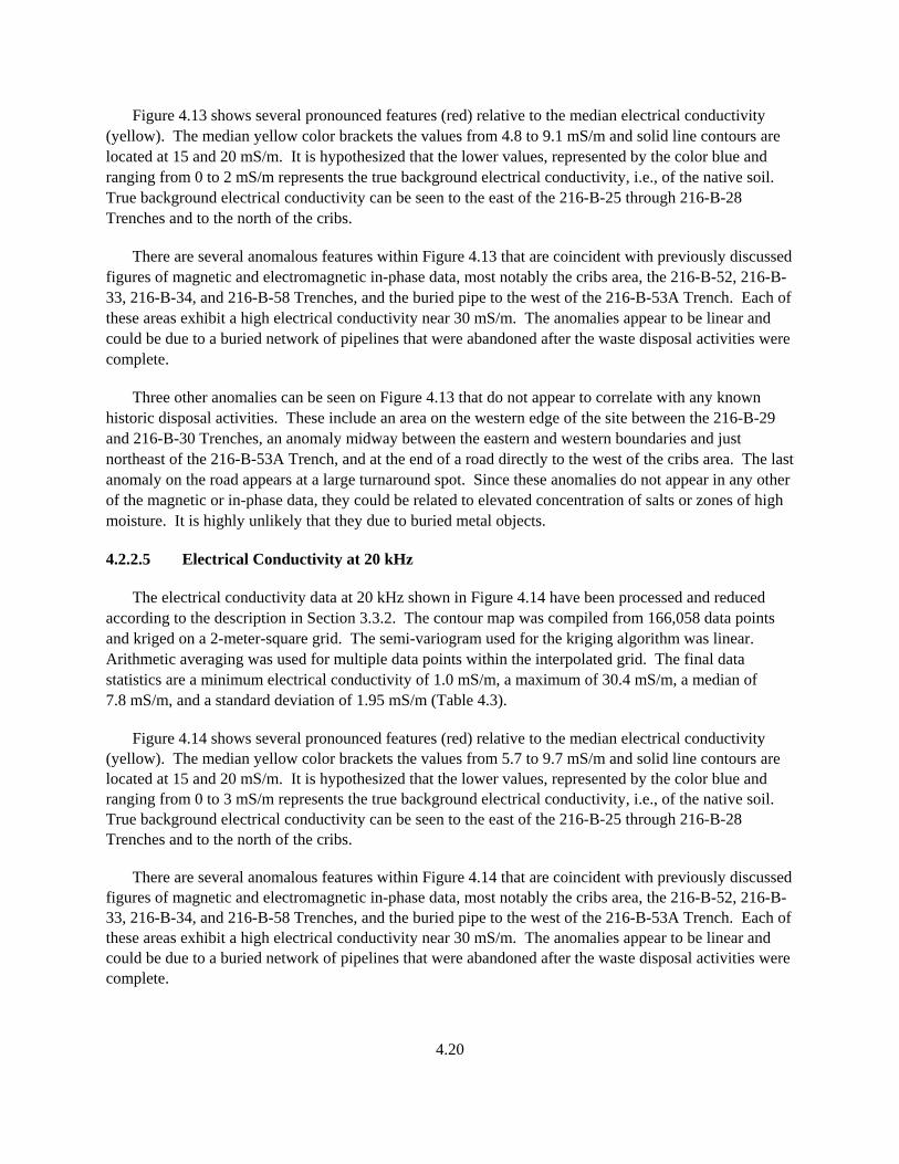
4.20
Figure 4.13 shows several pronounced features (red) relative to the median electrical conductivity (yellow). The median yellow color brackets the values from 4.8 to 9.1 mS/m and solid line contours are located at 15 and 20 mS/m. It is hypothesized that the lower values, represented by the color blue and ranging from 0 to 2 mS/m represents the true background electrical conductivity, i.e., of the native soil. True background electrical conductivity can be seen to the east of the 216-B-25 through 216-B-28 Trenches and to the north of the cribs.
There are several anomalous features within Figure 4.13 that are coincident with previously discussed figures of magnetic and electromagnetic in-phase data, most notably the cribs area, the 216-B-52, 216-B-33, 216-B-34, and 216-B-58 Trenches, and the buried pipe to the west of the 216-B-53A Trench. Each of these areas exhibit a high electrical conductivity near 30 mS/m. The anomalies appear to be linear and could be due to a buried network of pipelines that were abandoned after the waste disposal activities were complete.
Three other anomalies can be seen on Figure 4.13 that do not appear to correlate with any known historic disposal activities. These include an area on the western edge of the site between the 216-B-29 and 216-B-30 Trenches, an anomaly midway between the eastern and western boundaries and just northeast of the 216-B-53A Trench, and at the end of a road directly to the west of the cribs area. The last anomaly on the road appears at a large turnaround spot. Since these anomalies do not appear in any other of the magnetic or in-phase data, they could be related to elevated concentration of salts or zones of high moisture. It is highly unlikely that they due to buried metal objects.
4.2.2.5 Electrical Conductivity at 20 kHz
The electrical conductivity data at 20 kHz shown in Figure 4.14 have been processed and reduced according to the description in Section 3.3.2. The contour map was compiled from 166,058 data points and kriged on a 2-meter-square grid. The semi-variogram used for the kriging algorithm was linear. Arithmetic averaging was used for multiple data points within the interpolated grid. The final data statistics are a minimum electrical conductivity of 1.0 mS/m, a maximum of 30.4 mS/m, a median of 7.8 mS/m, and a standard deviation of 1.95 mS/m (Table 4.3).
Figure 4.14 shows several pronounced features (red) relative to the median electrical conductivity (yellow). The median yellow color brackets the values from 5.7 to 9.7 mS/m and solid line contours are located at 15 and 20 mS/m. It is hypothesized that the lower values, represented by the color blue and ranging from 0 to 3 mS/m represents the true background electrical conductivity, i.e., of the native soil. True background electrical conductivity can be seen to the east of the 216-B-25 through 216-B-28 Trenches and to the north of the cribs.
There are several anomalous features within Figure 4.14 that are coincident with previously discussed figures of magnetic and electromagnetic in-phase data, most notably the cribs area, the 216-B-52, 216-B-33, 216-B-34, and 216-B-58 Trenches, and the buried pipe to the west of the 216-B-53A Trench. Each of these areas exhibit a high electrical conductivity near 30 mS/m. The anomalies appear to be linear and could be due to a buried network of pipelines that were abandoned after the waste disposal activities were complete.
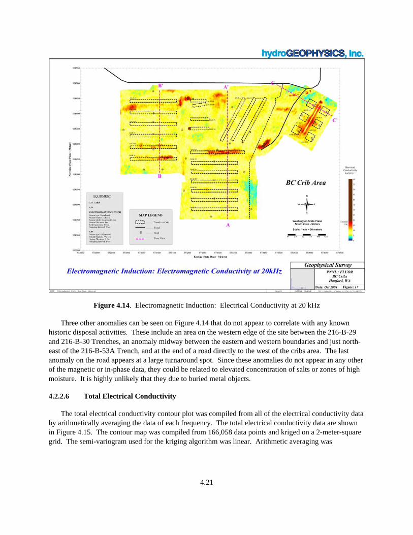
4.21
Figure 4.14. Electromagnetic Induction: Electrical Conductivity at 20 kHz
Three other anomalies can be seen on Figure 4.14 that do not appear to correlate with any known historic disposal activities. These include an area on the western edge of the site between the 216-B-29 and 216-B-30 Trenches, an anomaly midway between the eastern and western boundaries and just north-east of the 216-B-53A Trench, and at the end of a road directly to the west of the cribs area. The last anomaly on the road appears at a large turnaround spot. Since these anomalies do not appear in any other of the magnetic or in-phase data, they could be related to elevated concentration of salts or zones of high moisture. It is highly unlikely that they due to buried metal objects.
4.2.2.6 Total Electrical Conductivity
The total electrical conductivity contour plot was compiled from all of the electrical conductivity data by arithmetically averaging the data of each frequency. The total electrical conductivity data are shown in Figure 4.15. The contour map was compiled from 166,058 data points and kriged on a 2-meter-square grid. The semi-variogram used for the kriging algorithm was linear. Arithmetic averaging was
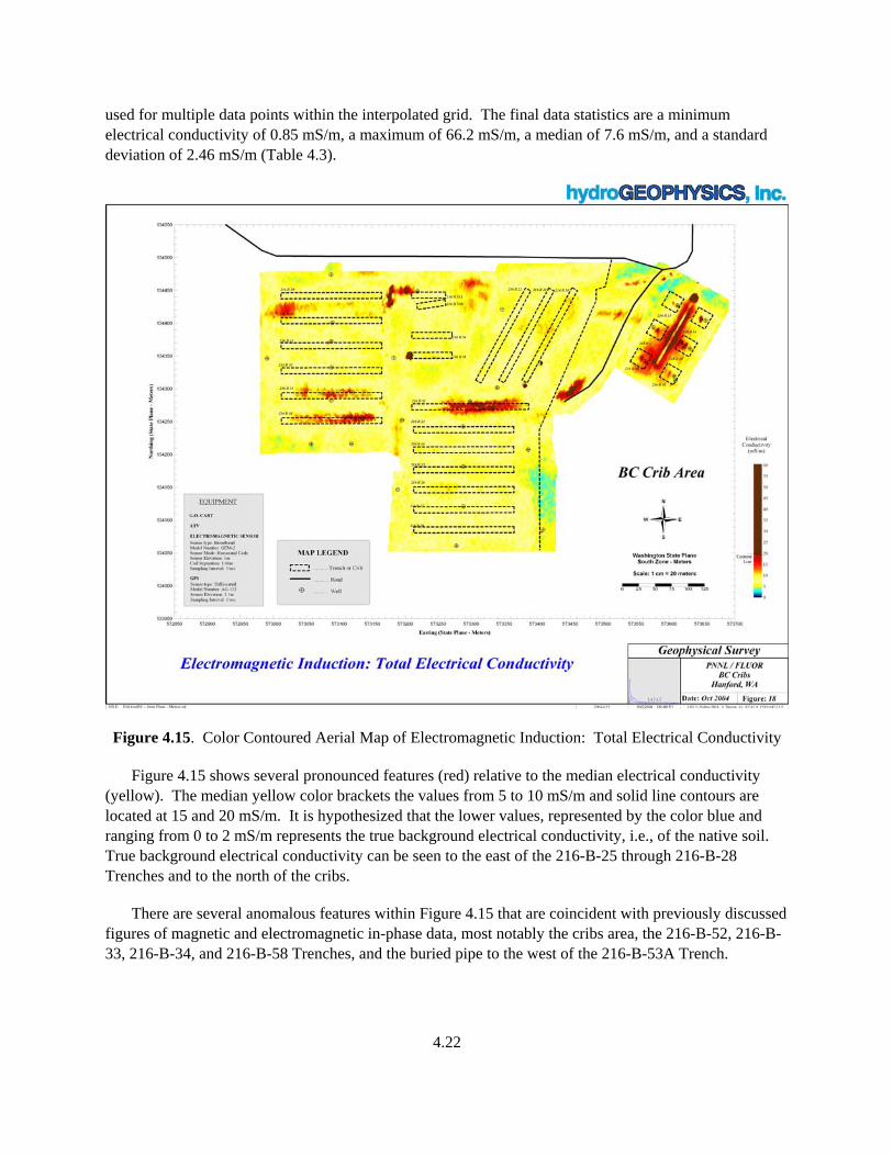
4.22
used for multiple data points within the interpolated grid. The final data statistics are a minimum electrical conductivity of 0.85 mS/m, a maximum of 66.2 mS/m, a median of 7.6 mS/m, and a standard deviation of 2.46 mS/m (Table 4.3).
Figure 4.15. Color Contoured Aerial Map of Electromagnetic Induction: Total Electrical Conductivity
Figure 4.15 shows several pronounced features (red) relative to the median electrical conductivity (yellow). The median yellow color brackets the values from 5 to 10 mS/m and solid line contours are located at 15 and 20 mS/m. It is hypothesized that the lower values, represented by the color blue and ranging from 0 to 2 mS/m represents the true background electrical conductivity, i.e., of the native soil. True background electrical conductivity can be seen to the east of the 216-B-25 through 216-B-28 Trenches and to the north of the cribs.
There are several anomalous features within Figure 4.15 that are coincident with previously discussed figures of magnetic and electromagnetic in-phase data, most notably the cribs area, the 216-B-52, 216-B-33, 216-B-34, and 216-B-58 Trenches, and the buried pipe to the west of the 216-B-53A Trench.
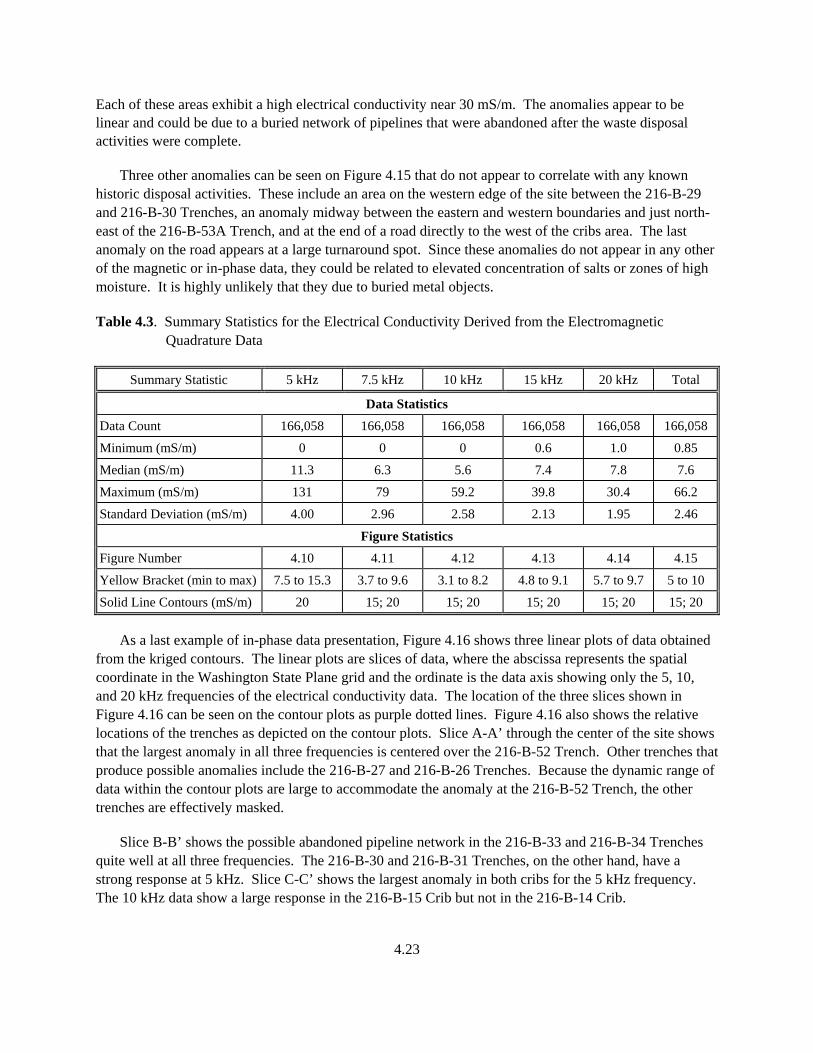
4.23
Each of these areas exhibit a high electrical conductivity near 30 mS/m. The anomalies appear to be linear and could be due to a buried network of pipelines that were abandoned after the waste disposal activities were complete.
Three other anomalies can be seen on Figure 4.15 that do not appear to correlate with any known historic disposal activities. These include an area on the western edge of the site between the 216-B-29 and 216-B-30 Trenches, an anomaly midway between the eastern and western boundaries and just north-east of the 216-B-53A Trench, and at the end of a road directly to the west of the cribs area. The last anomaly on the road appears at a large turnaround spot. Since these anomalies do not appear in any other of the magnetic or in-phase data, they could be related to elevated concentration of salts or zones of high moisture. It is highly unlikely that they due to buried metal objects.
Table 4.3. Summary Statistics for the Electrical Conductivity Derived from the Electromagnetic Quadrature Data
Summary Statistic 5 kHz 7.5 kHz 10 kHz 15 kHz 20 kHz Total
Data Statistics
Data Count 166,058 166,058 166,058 166,058 166,058 166,058
Minimum (mS/m) 0 0 0 0.6 1.0 0.85
Median (mS/m) 11.3 6.3 5.6 7.4 7.8 7.6
Maximum (mS/m) 131 79 59.2 39.8 30.4 66.2
Standard Deviation (mS/m) 4.00 2.96 2.58 2.13 1.95 2.46
Figure Statistics
Figure Number 4.10 4.11 4.12 4.13 4.14 4.15
Yellow Bracket (min to max) 7.5 to 15.3 3.7 to 9.6 3.1 to 8.2 4.8 to 9.1 5.7 to 9.7 5 to 10
Solid Line Contours (mS/m) 20 15; 20 15; 20 15; 20 15; 20 15; 20
As a last example of in-phase data presentation, Figure 4.16 shows three linear plots of data obtained from the kriged contours. The linear plots are slices of data, where the abscissa represents the spatial coordinate in the Washington State Plane grid and the ordinate is the data axis showing only the 5, 10, and 20 kHz frequencies of the electrical conductivity data. The location of the three slices shown in Figure 4.16 can be seen on the contour plots as purple dotted lines. Figure 4.16 also shows the relative locations of the trenches as depicted on the contour plots. Slice A-A’ through the center of the site shows that the largest anomaly in all three frequencies is centered over the 216-B-52 Trench. Other trenches that produce possible anomalies include the 216-B-27 and 216-B-26 Trenches. Because the dynamic range of data within the contour plots are large to accommodate the anomaly at the 216-B-52 Trench, the other trenches are effectively masked.
Slice B-B’ shows the possible abandoned pipeline network in the 216-B-33 and 216-B-34 Trenches quite well at all three frequencies. The 216-B-30 and 216-B-31 Trenches, on the other hand, have a strong response at 5 kHz. Slice C-C’ shows the largest anomaly in both cribs for the 5 kHz frequency. The 10 kHz data show a large response in the 216-B-15 Crib but not in the 216-B-14 Crib.
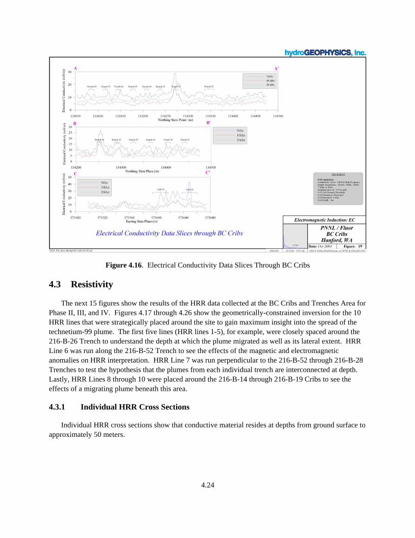
4.24
Figure 4.16. Electrical Conductivity Data Slices Through BC Cribs
4.3 Resistivity
The next 15 figures show the results of the HRR data collected at the BC Cribs and Trenches Area for Phase II, III, and IV. Figures 4.17 through 4.26 show the geometrically-constrained inversion for the 10 HRR lines that were strategically placed around the site to gain maximum insight into the spread of the technetium-99 plume. The first five lines (HRR lines 1-5), for example, were closely spaced around the 216-B-26 Trench to understand the depth at which the plume migrated as well as its lateral extent. HRR Line 6 was run along the 216-B-52 Trench to see the effects of the magnetic and electromagnetic anomalies on HRR interpretation. HRR Line 7 was run perpendicular to the 216-B-52 through 216-B-28 Trenches to test the hypothesis that the plumes from each individual trench are interconnected at depth. Lastly, HRR Lines 8 through 10 were placed around the 216-B-14 through 216-B-19 Cribs to see the effects of a migrating plume beneath this area.
4.3.1 Individual HRR Cross Sections
Individual HRR cross sections show that conductive material resides at depths from ground surface to approximately 50 meters.
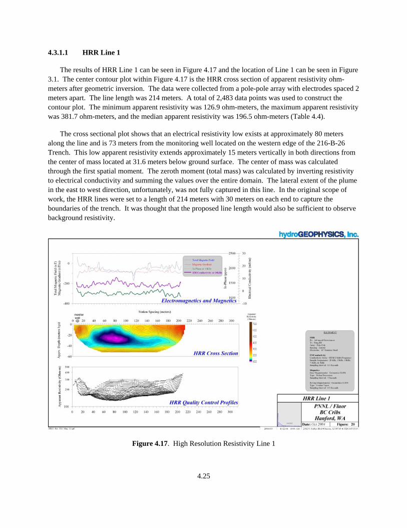
4.25
4.3.1.1 HRR Line 1
The results of HRR Line 1 can be seen in Figure 4.17 and the location of Line 1 can be seen in Figure 3.1. The center contour plot within Figure 4.17 is the HRR cross section of apparent resistivity ohm-meters after geometric inversion. The data were collected from a pole-pole array with electrodes spaced 2 meters apart. The line length was 214 meters. A total of 2,483 data points was used to construct the contour plot. The minimum apparent resistivity was 126.9 ohm-meters, the maximum apparent resistivity was 381.7 ohm-meters, and the median apparent resistivity was 196.5 ohm-meters (Table 4.4).
The cross sectional plot shows that an electrical resistivity low exists at approximately 80 meters along the line and is 73 meters from the monitoring well located on the western edge of the 216-B-26 Trench. This low apparent resistivity extends approximately 15 meters vertically in both directions from the center of mass located at 31.6 meters below ground surface. The center of mass was calculated through the first spatial moment. The zeroth moment (total mass) was calculated by inverting resistivity to electrical conductivity and summing the values over the entire domain. The lateral extent of the plume in the east to west direction, unfortunately, was not fully captured in this line. In the original scope of work, the HRR lines were set to a length of 214 meters with 30 meters on each end to capture the boundaries of the trench. It was thought that the proposed line length would also be sufficient to observe background resistivity.
Figure 4.17. High Resolution Resistivity Line 1
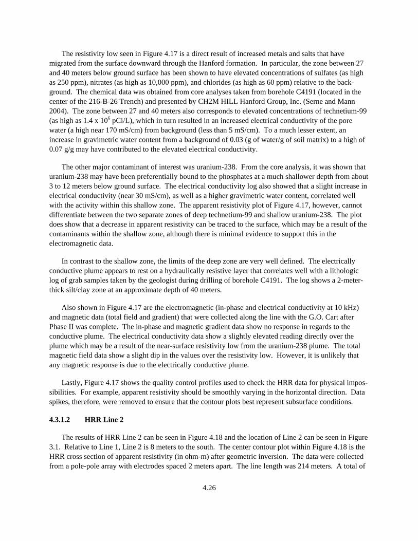
4.26
The resistivity low seen in Figure 4.17 is a direct result of increased metals and salts that have migrated from the surface downward through the Hanford formation. In particular, the zone between 27 and 40 meters below ground surface has been shown to have elevated concentrations of sulfates (as high as 250 ppm), nitrates (as high as 10,000 ppm), and chlorides (as high as 60 ppm) relative to the back-ground. The chemical data was obtained from core analyses taken from borehole C4191 (located in the center of the 216-B-26 Trench) and presented by CH2M HILL Hanford Group, Inc. (Serne and Mann 2004). The zone between 27 and 40 meters also corresponds to elevated concentrations of technetium-99 (as high as 1.4 x 10⁶ pCi/L), which in turn resulted in an increased electrical conductivity of the pore water (a high near 170 mS/cm) from background (less than 5 mS/cm). To a much lesser extent, an increase in gravimetric water content from a background of 0.03 (g of water/g of soil matrix) to a high of 0.07 g/g may have contributed to the elevated electrical conductivity.
The other major contaminant of interest was uranium-238. From the core analysis, it was shown that uranium-238 may have been preferentially bound to the phosphates at a much shallower depth from about 3 to 12 meters below ground surface. The electrical conductivity log also showed that a slight increase in electrical conductivity (near 30 mS/cm), as well as a higher gravimetric water content, correlated well with the activity within this shallow zone. The apparent resistivity plot of Figure 4.17, however, cannot differentiate between the two separate zones of deep technetium-99 and shallow uranium-238. The plot does show that a decrease in apparent resistivity can be traced to the surface, which may be a result of the contaminants within the shallow zone, although there is minimal evidence to support this in the electromagnetic data.
In contrast to the shallow zone, the limits of the deep zone are very well defined. The electrically conductive plume appears to rest on a hydraulically resistive layer that correlates well with a lithologic log of grab samples taken by the geologist during drilling of borehole C4191. The log shows a 2-meter-thick silt/clay zone at an approximate depth of 40 meters.
Also shown in Figure 4.17 are the electromagnetic (in-phase and electrical conductivity at 10 kHz) and magnetic data (total field and gradient) that were collected along the line with the G.O. Cart after Phase II was complete. The in-phase and magnetic gradient data show no response in regards to the conductive plume. The electrical conductivity data show a slightly elevated reading directly over the plume which may be a result of the near-surface resistivity low from the uranium-238 plume. The total magnetic field data show a slight dip in the values over the resistivity low. However, it is unlikely that any magnetic response is due to the electrically conductive plume.
Lastly, Figure 4.17 shows the quality control profiles used to check the HRR data for physical impos-sibilities. For example, apparent resistivity should be smoothly varying in the horizontal direction. Data spikes, therefore, were removed to ensure that the contour plots best represent subsurface conditions.
4.3.1.2 HRR Line 2
The results of HRR Line 2 can be seen in Figure 4.18 and the location of Line 2 can be seen in Figure 3.1. Relative to Line 1, Line 2 is 8 meters to the south. The center contour plot within Figure 4.18 is the HRR cross section of apparent resistivity (in ohm-m) after geometric inversion. The data were collected from a pole-pole array with electrodes spaced 2 meters apart. The line length was 214 meters. A total of
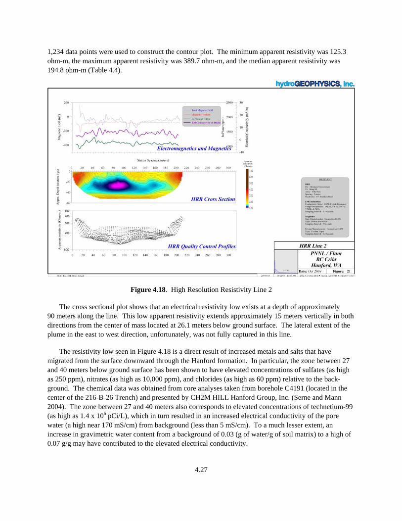
4.27
1,234 data points were used to construct the contour plot. The minimum apparent resistivity was 125.3 ohm-m, the maximum apparent resistivity was 389.7 ohm-m, and the median apparent resistivity was 194.8 ohm-m (Table 4.4).
Figure 4.18. High Resolution Resistivity Line 2
The cross sectional plot shows that an electrical resistivity low exists at a depth of approximately 90 meters along the line. This low apparent resistivity extends approximately 15 meters vertically in both directions from the center of mass located at 26.1 meters below ground surface. The lateral extent of the plume in the east to west direction, unfortunately, was not fully captured in this line.
The resistivity low seen in Figure 4.18 is a direct result of increased metals and salts that have migrated from the surface downward through the Hanford formation. In particular, the zone between 27 and 40 meters below ground surface has been shown to have elevated concentrations of sulfates (as high as 250 ppm), nitrates (as high as 10,000 ppm), and chlorides (as high as 60 ppm) relative to the back-ground. The chemical data was obtained from core analyses taken from borehole C4191 (located in the center of the 216-B-26 Trench) and presented by CH2M HILL Hanford Group, Inc. (Serne and Mann 2004). The zone between 27 and 40 meters also corresponds to elevated concentrations of technetium-99 (as high as 1.4 x 10⁶ pCi/L), which in turn resulted in an increased electrical conductivity of the pore water (a high near 170 mS/cm) from background (less than 5 mS/cm). To a much lesser extent, an increase in gravimetric water content from a background of 0.03 (g of water/g of soil matrix) to a high of 0.07 g/g may have contributed to the elevated electrical conductivity.
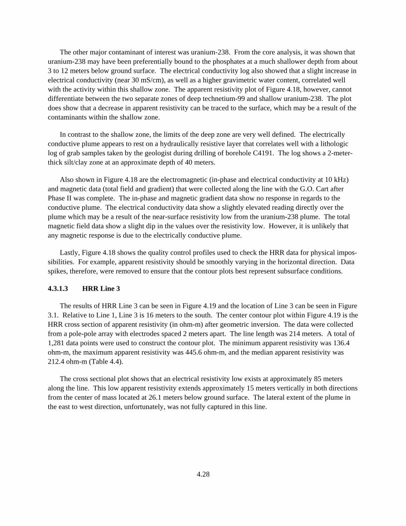
4.28
The other major contaminant of interest was uranium-238. From the core analysis, it was shown that uranium-238 may have been preferentially bound to the phosphates at a much shallower depth from about 3 to 12 meters below ground surface. The electrical conductivity log also showed that a slight increase in electrical conductivity (near 30 mS/cm), as well as a higher gravimetric water content, correlated well with the activity within this shallow zone. The apparent resistivity plot of Figure 4.18, however, cannot differentiate between the two separate zones of deep technetium-99 and shallow uranium-238. The plot does show that a decrease in apparent resistivity can be traced to the surface, which may be a result of the contaminants within the shallow zone.
In contrast to the shallow zone, the limits of the deep zone are very well defined. The electrically conductive plume appears to rest on a hydraulically resistive layer that correlates well with a lithologic log of grab samples taken by the geologist during drilling of borehole C4191. The log shows a 2-meter-thick silt/clay zone at an approximate depth of 40 meters.
Also shown in Figure 4.18 are the electromagnetic (in-phase and electrical conductivity at 10 kHz) and magnetic data (total field and gradient) that were collected along the line with the G.O. Cart after Phase II was complete. The in-phase and magnetic gradient data show no response in regards to the conductive plume. The electrical conductivity data show a slightly elevated reading directly over the plume which may be a result of the near-surface resistivity low from the uranium-238 plume. The total magnetic field data show a slight dip in the values over the resistivity low. However, it is unlikely that any magnetic response is due to the electrically conductive plume.
Lastly, Figure 4.18 shows the quality control profiles used to check the HRR data for physical impos-sibilities. For example, apparent resistivity should be smoothly varying in the horizontal direction. Data spikes, therefore, were removed to ensure that the contour plots best represent subsurface conditions.
4.3.1.3 HRR Line 3
The results of HRR Line 3 can be seen in Figure 4.19 and the location of Line 3 can be seen in Figure 3.1. Relative to Line 1, Line 3 is 16 meters to the south. The center contour plot within Figure 4.19 is the HRR cross section of apparent resistivity (in ohm-m) after geometric inversion. The data were collected from a pole-pole array with electrodes spaced 2 meters apart. The line length was 214 meters. A total of 1,281 data points were used to construct the contour plot. The minimum apparent resistivity was 136.4 ohm-m, the maximum apparent resistivity was 445.6 ohm-m, and the median apparent resistivity was 212.4 ohm-m (Table 4.4).
The cross sectional plot shows that an electrical resistivity low exists at approximately 85 meters along the line. This low apparent resistivity extends approximately 15 meters vertically in both directions from the center of mass located at 26.1 meters below ground surface. The lateral extent of the plume in the east to west direction, unfortunately, was not fully captured in this line.
4.29
Figure 4.19. High Resolution Resistivity Line 3
The resistivity low seen in Figure 4.19 is a direct result of increased metals and salts that have migrated from the surface downward through the Hanford formation. In particular, the zone between 27 and 40 meters below ground surface has been shown to have elevated concentrations of sulfates (as high as 250 ppm), nitrates (as high as 10,000 ppm), and chlorides (as high as 60 ppm) relative to the back-ground. The chemical data was obtained from core analyses taken from borehole C4191 (located in the center of the 216-B-26 Trench) and presented by CH2M HILL Hanford Group, Inc. (Serne and Mann 2004). The zone between 27 and 40 meters also corresponds to elevated concentrations of technetium-99 (as high as 1.4 x 10⁶ pCi/L), which in turn resulted in an increased electrical conductivity of the pore water (a high near 170 mS/cm) from background (less than 5 mS/cm). To a much lesser extent, an increase in gravimetric water content from a background of 0.03 (g of water/g of soil matrix) to a high of 0.07 g/g may have contributed to the elevated electrical conductivity.
The other major contaminant of interest was uranium-238. From the core analysis, it was shown that uranium-238 may have been preferentially bound to the phosphates at a much shallower depth from about 3 to 12 meters below ground surface. The electrical conductivity log also showed that a slight increase in electrical conductivity (near 30 mS/cm), as well as a higher gravimetric water content, correlated well with the activity within this shallow zone. The apparent resistivity plot of Figure 4.19, however, does not show any near-surface resistivity low due to the uranium-238. Migration of this radionuclide may have been confined more closely to the trench location and its lateral extent was minimized. Additionally, the electrically conductive plume appears to rest on a hydraulically resistive layer that correlates well with a
4.30
lithologic log of grab samples taken by the geologist during drilling of borehole C4191. The log shows a 2-meter silt/clay zone at an approximate depth of 40 meters.
Also shown in Figure 4.19 are the electromagnetic (in-phase and electrical conductivity at 10 kHz) and magnetic data (total field and gradient) that were collected along the line with the G.O. Cart after Phase II was complete. The in-phase data show no response in regards to the conductive plume. The electrical conductivity data also does not show any significant change directly over the plume as seen in Figures 4.17 and 4.18. The total magnetic field and magnetic gradient data show a large dip in values over the resistivity low. This dip, however, is due to a fence post that designated the clean area from the soil contamination area.
Lastly, Figure 4.19 shows the quality control profiles used to check the HRR data for physical impos-sibilities. For example, apparent resistivity should be smoothly varying in the horizontal direction. Data spikes, therefore, were removed to ensure that the contour plots best represent subsurface conditions.
4.3.1.4 HRR Line 4
The results of HRR Line 4 can be seen in Figure 4.20 and the location of Line 4 can be seen in Figure 3.1. Relative to Line 1, Line 3 is 8 meters to the north. The center contour plot within Figure 4.20 is the HRR cross section of apparent resistivity (in ohm-m) after geometric inversion. The data were collected from a pole-pole array with electrodes spaced 2 meters apart. The line length was 314 meters. A total of 1,909 data points were used to construct the contour plot. The minimum apparent resistivity was 130.7 ohm-m, the maximum apparent resistivity was 747.9 ohm-m, and the median apparent resistivity was 224.9 ohm-m (Table 4.4).
The cross sectional plot shows that an electrical resistivity low exists at approximately 90 meters along the line. This low apparent resistivity extends approximately 15 meters vertically in both directions from the center of mass located at 27.6 meters below ground surface. The lateral extent of the plume in the western direction, unfortunately, was not fully captured in this line. To the east, the line was extended an additional 100 meters compared to previous lines to map more of the background and to find the edge of the plume.
The resistivity low seen in Figure 4.20 is a direct result of increased metals and salts that have migrated from the surface downward through the Hanford formation. In particular, the zone between 27 and 40 meters below ground surface has been shown to have elevated concentrations of sulfates (as high as 250 ppm), nitrates (as high as 10,000 ppm), and chlorides (as high as 60 ppm) relative to the back-ground. The chemical data was obtained from core analyses taken from borehole C4191 (located in the center of the 216-B-26 Trench) and presented by CH2M HILL Hanford Group, Inc. (Serne and Mann 2004). The zone between 27 and 40 meters also corresponds to elevated concentrations of technetium-99 (as high as 1.4 x 10⁶ pCi/L), which in turn resulted in an increased electrical conductivity of the pore water (a high near 170 mS/cm) from background (less than 5 mS/cm). To a much lesser extent, an increase in gravimetric water content from a background of 0.03 (g of water/g of soil matrix) to a high of 0.07 g/g may have contributed to the elevated electrical conductivity.
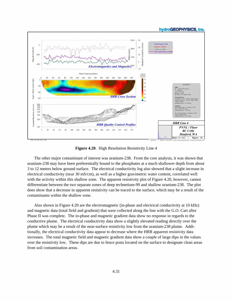
4.31
Figure 4.20. High Resolution Resistivity Line 4
The other major contaminant of interest was uranium-238. From the core analysis, it was shown that uranium-238 may have been preferentially bound to the phosphates at a much shallower depth from about 3 to 12 meters below ground surface. The electrical conductivity log also showed that a slight increase in electrical conductivity (near 30 mS/cm), as well as a higher gravimetric water content, correlated well with the activity within this shallow zone. The apparent resistivity plot of Figure 4.20, however, cannot differentiate between the two separate zones of deep technetium-99 and shallow uranium-238. The plot does show that a decrease in apparent resistivity can be traced to the surface, which may be a result of the contaminants within the shallow zone.
Also shown in Figure 4.20 are the electromagnetic (in-phase and electrical conductivity at 10 kHz) and magnetic data (total field and gradient) that were collected along the line with the G.O. Cart after Phase II was complete. The in-phase and magnetic gradient data show no response in regards to the conductive plume. The electrical conductivity data show a slightly elevated reading directly over the plume which may be a result of the near-surface resistivity low from the uranium-238 plume. Addi-tionally, the electrical conductivity data appear to decrease where the HRR apparent resistivity data increases. The total magnetic field and magnetic gradient data show a couple of large dips in the values over the resistivity low. These dips are due to fence posts located on the surface to designate clean areas from soil contamination areas.
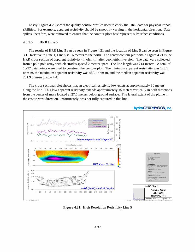
4.32
Lastly, Figure 4.20 shows the quality control profiles used to check the HRR data for physical impos-sibilities. For example, apparent resistivity should be smoothly varying in the horizontal direction. Data spikes, therefore, were removed to ensure that the contour plots best represent subsurface conditions.
4.3.1.5 HRR Line 5
The results of HRR Line 5 can be seen in Figure 4.21 and the location of Line 5 can be seen in Figure 3.1. Relative to Line 1, Line 5 is 16 meters to the north. The center contour plot within Figure 4.21 is the HRR cross section of apparent resistivity (in ohm-m) after geometric inversion. The data were collected from a pole-pole array with electrodes spaced 2 meters apart. The line length was 214 meters. A total of 1,297 data points were used to construct the contour plot. The minimum apparent resistivity was 123.1 ohm-m, the maximum apparent resistivity was 460.1 ohm-m, and the median apparent resistivity was 201.9 ohm-m (Table 4.4).
The cross sectional plot shows that an electrical resistivity low exists at approximately 80 meters along the line. This low apparent resistivity extends approximately 15 meters vertically in both directions from the center of mass located at 27.5 meters below ground surface. The lateral extent of the plume in the east to west direction, unfortunately, was not fully captured in this line.
Figure 4.21. High Resolution Resistivity Line 5
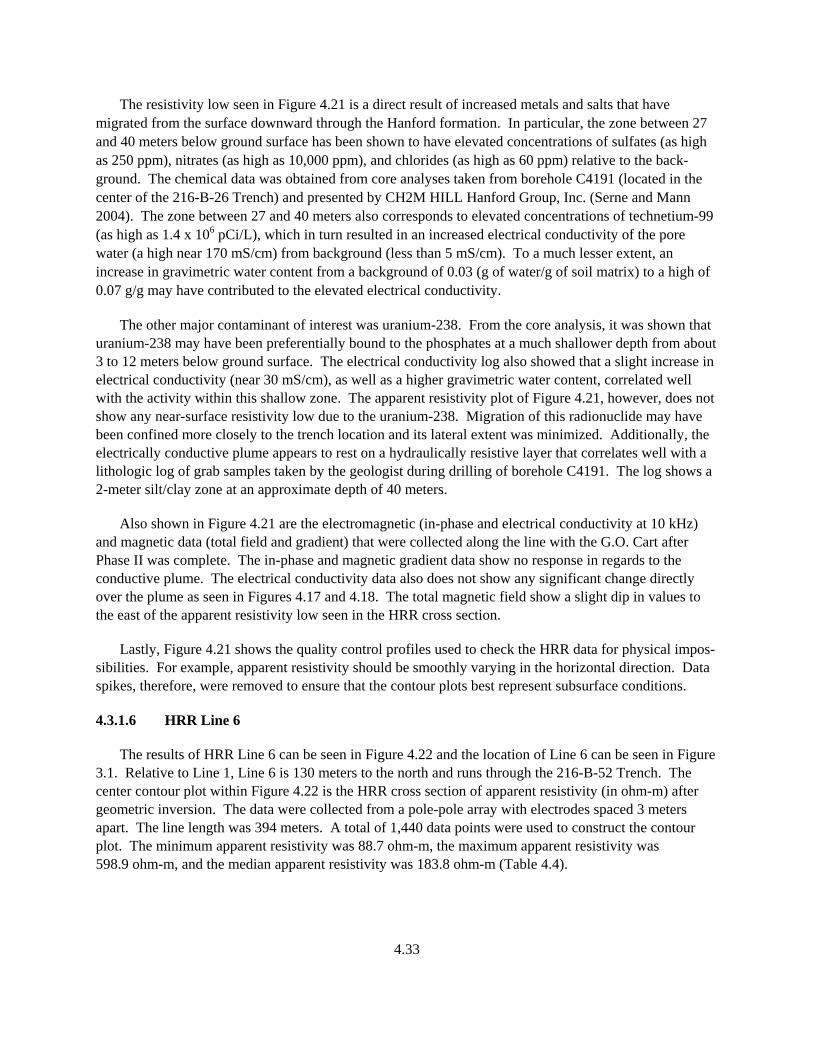
4.33
The resistivity low seen in Figure 4.21 is a direct result of increased metals and salts that have migrated from the surface downward through the Hanford formation. In particular, the zone between 27 and 40 meters below ground surface has been shown to have elevated concentrations of sulfates (as high as 250 ppm), nitrates (as high as 10,000 ppm), and chlorides (as high as 60 ppm) relative to the back-ground. The chemical data was obtained from core analyses taken from borehole C4191 (located in the center of the 216-B-26 Trench) and presented by CH2M HILL Hanford Group, Inc. (Serne and Mann 2004). The zone between 27 and 40 meters also corresponds to elevated concentrations of technetium-99 (as high as 1.4 x 10⁶ pCi/L), which in turn resulted in an increased electrical conductivity of the pore water (a high near 170 mS/cm) from background (less than 5 mS/cm). To a much lesser extent, an increase in gravimetric water content from a background of 0.03 (g of water/g of soil matrix) to a high of 0.07 g/g may have contributed to the elevated electrical conductivity.
The other major contaminant of interest was uranium-238. From the core analysis, it was shown that uranium-238 may have been preferentially bound to the phosphates at a much shallower depth from about 3 to 12 meters below ground surface. The electrical conductivity log also showed that a slight increase in electrical conductivity (near 30 mS/cm), as well as a higher gravimetric water content, correlated well with the activity within this shallow zone. The apparent resistivity plot of Figure 4.21, however, does not show any near-surface resistivity low due to the uranium-238. Migration of this radionuclide may have been confined more closely to the trench location and its lateral extent was minimized. Additionally, the electrically conductive plume appears to rest on a hydraulically resistive layer that correlates well with a lithologic log of grab samples taken by the geologist during drilling of borehole C4191. The log shows a 2-meter silt/clay zone at an approximate depth of 40 meters.
Also shown in Figure 4.21 are the electromagnetic (in-phase and electrical conductivity at 10 kHz) and magnetic data (total field and gradient) that were collected along the line with the G.O. Cart after Phase II was complete. The in-phase and magnetic gradient data show no response in regards to the conductive plume. The electrical conductivity data also does not show any significant change directly over the plume as seen in Figures 4.17 and 4.18. The total magnetic field show a slight dip in values to the east of the apparent resistivity low seen in the HRR cross section.
Lastly, Figure 4.21 shows the quality control profiles used to check the HRR data for physical impos-sibilities. For example, apparent resistivity should be smoothly varying in the horizontal direction. Data spikes, therefore, were removed to ensure that the contour plots best represent subsurface conditions.
4.3.1.6 HRR Line 6
The results of HRR Line 6 can be seen in Figure 4.22 and the location of Line 6 can be seen in Figure 3.1. Relative to Line 1, Line 6 is 130 meters to the north and runs through the 216-B-52 Trench. The center contour plot within Figure 4.22 is the HRR cross section of apparent resistivity (in ohm-m) after geometric inversion. The data were collected from a pole-pole array with electrodes spaced 3 meters apart. The line length was 394 meters. A total of 1,440 data points were used to construct the contour plot. The minimum apparent resistivity was 88.7 ohm-m, the maximum apparent resistivity was 598.9 ohm-m, and the median apparent resistivity was 183.8 ohm-m (Table 4.4).
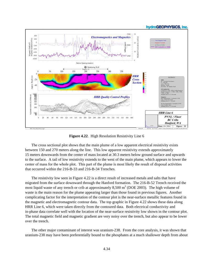
4.34
Figure 4.22. High Resolution Resistivity Line 6
The cross sectional plot shows that the main plume of a low apparent electrical resistivity exists between 150 and 270 meters along the line. This low apparent resistivity extends approximately 15 meters downwards from the center of mass located at 30.3 meters below ground surface and upwards to the surface. A tail of low resistivity extends to the west of the main plume, which appears to lower the center of mass for the whole plot. This part of the plume is most likely the result of disposal activities that occurred within the 216-B-33 and 216-B-34 Trenches.
The resistivity low seen in Figure 4.22 is a direct result of increased metals and salts that have migrated from the surface downward through the Hanford formation. The 216-B-52 Trench received the most liquid waste of any trench or crib at approximately 8,500 m3 (DOE 2003). The high volume of waste is the main reason for the plume appearing larger than those found in previous figures. Another complicating factor for the interpretation of the contour plot is the near-surface metallic features found in the magnetic and electromagnetic contour data. The top graphic in Figure 4.22 shows these data along HRR Line 6, which were taken directly from the contoured data. Both electrical conductivity and in-phase data correlate well with the location of the near-surface resistivity low shown in the contour plot. The total magnetic field and magnetic gradient are very noisy over the trench, but also appear to be lower over the trench.
The other major contaminant of interest was uranium-238. From the core analysis, it was shown that uranium-238 may have been preferentially bound to the phosphates at a much shallower depth from about
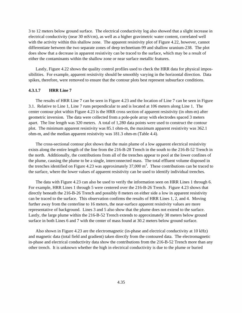
4.35
3 to 12 meters below ground surface. The electrical conductivity log also showed that a slight increase in electrical conductivity (near 30 mS/cm), as well as a higher gravimetric water content, correlated well with the activity within this shallow zone. The apparent resistivity plot of Figure 4.22, however, cannot differentiate between the two separate zones of deep technetium-99 and shallow uranium-238. The plot does show that a decrease in apparent resistivity can be traced to the surface, which may be a result of either the contaminants within the shallow zone or near surface metallic features.
Lastly, Figure 4.22 shows the quality control profiles used to check the HRR data for physical impos-sibilities. For example, apparent resistivity should be smoothly varying in the horizontal direction. Data spikes, therefore, were removed to ensure that the contour plots best represent subsurface conditions.
4.3.1.7 HRR Line 7
The results of HRR Line 7 can be seen in Figure 4.23 and the location of Line 7 can be seen in Figure 3.1. Relative to Line 1, Line 7 runs perpendicular to and is located at 106 meters along Line 1. The center contour plot within Figure 4.23 is the HRR cross section of apparent resistivity (in ohm-m) after geometric inversion. The data were collected from a pole-pole array with electrodes spaced 3 meters apart. The line length was 320 meters. A total of 1,280 data points were used to construct the contour plot. The minimum apparent resistivity was 85.1 ohm-m, the maximum apparent resistivity was 362.1 ohm-m, and the median apparent resistivity was 181.3 ohm-m (Table 4.4).
The cross-sectional contour plot shows that the main plume of a low apparent electrical resistivity exists along the entire length of the line from the 216-B-28 Trench in the south to the 216-B-52 Trench in the north. Additionally, the contributions from all of the trenches appear to pool at the lower confines of the plume, causing the plume to be a single, interconnected mass. The total effluent volume disposed in the trenches identified on Figure 4.23 was approximately 37,000 m3. These contributions can be traced to the surface, where the lower values of apparent resistivity can be used to identify individual trenches.
The data with Figure 4.23 can also be used to verify the information seen on HRR Lines 1 through 6. For example, HRR Lines 1 through 5 were centered over the 216-B-26 Trench. Figure 4.23 shows that directly beneath the 216-B-26 Trench and possibly 8 meters on either side a low in apparent resistivity can be traced to the surface. This observation confirms the results of HRR Lines 1, 2, and 4. Moving further away from the centerline to 16 meters, the near-surface apparent resistivity values are more representative of background. Lines 3 and 5 also show that the plume does not extend to the surface. Lastly, the large plume within the 216-B-52 Trench extends to approximately 38 meters below ground surface in both Lines 6 and 7 with the center of mass found at 30.2 meters below ground surface.
Also shown in Figure 4.23 are the electromagnetic (in-phase and electrical conductivity at 10 kHz) and magnetic data (total field and gradient) taken directly from the contoured data. The electromagnetic in-phase and electrical conductivity data show the contributions from the 216-B-52 Trench more than any other trench. It is unknown whether the high in electrical conductivity is due to the plume or buried
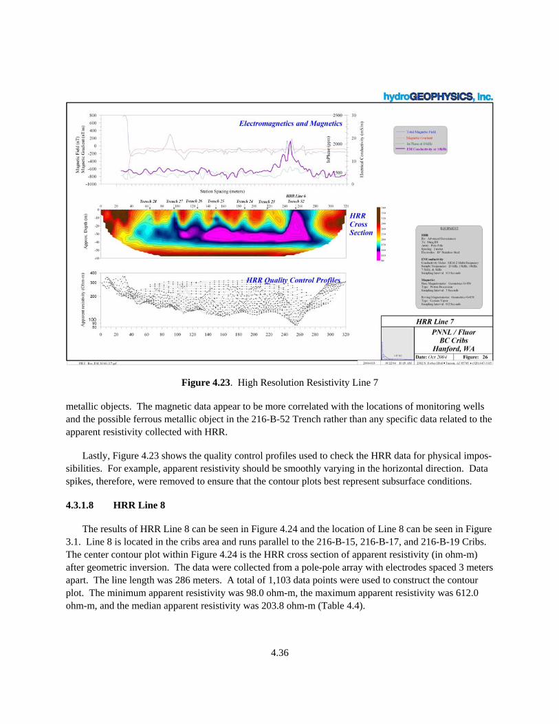
4.36
Figure 4.23. High Resolution Resistivity Line 7
metallic objects. The magnetic data appear to be more correlated with the locations of monitoring wells and the possible ferrous metallic object in the 216-B-52 Trench rather than any specific data related to the apparent resistivity collected with HRR.
Lastly, Figure 4.23 shows the quality control profiles used to check the HRR data for physical impos-sibilities. For example, apparent resistivity should be smoothly varying in the horizontal direction. Data spikes, therefore, were removed to ensure that the contour plots best represent subsurface conditions.
4.3.1.8 HRR Line 8
The results of HRR Line 8 can be seen in Figure 4.24 and the location of Line 8 can be seen in Figure 3.1. Line 8 is located in the cribs area and runs parallel to the 216-B-15, 216-B-17, and 216-B-19 Cribs. The center contour plot within Figure 4.24 is the HRR cross section of apparent resistivity (in ohm-m) after geometric inversion. The data were collected from a pole-pole array with electrodes spaced 3 meters apart. The line length was 286 meters. A total of 1,103 data points were used to construct the contour plot. The minimum apparent resistivity was 98.0 ohm-m, the maximum apparent resistivity was 612.0 ohm-m, and the median apparent resistivity was 203.8 ohm-m (Table 4.4).
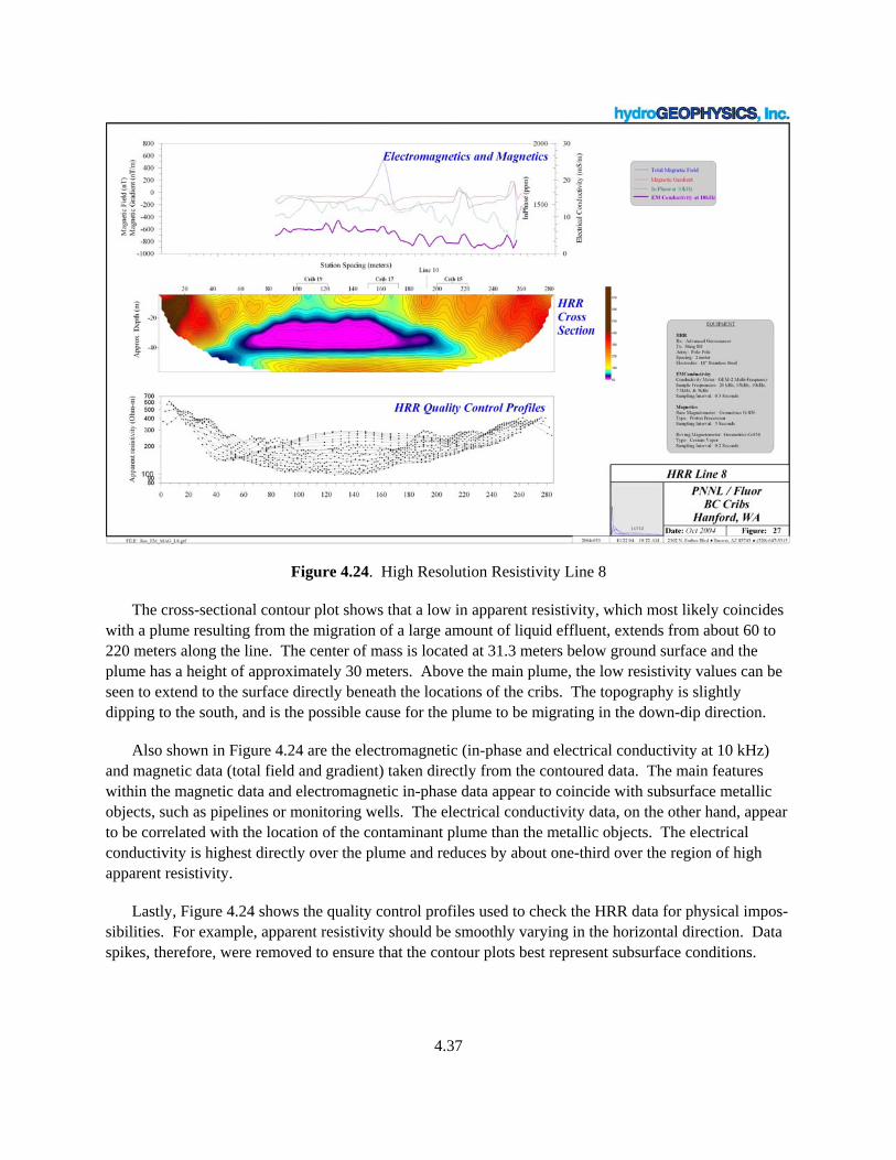
4.37
Figure 4.24. High Resolution Resistivity Line 8
The cross-sectional contour plot shows that a low in apparent resistivity, which most likely coincides with a plume resulting from the migration of a large amount of liquid effluent, extends from about 60 to 220 meters along the line. The center of mass is located at 31.3 meters below ground surface and the plume has a height of approximately 30 meters. Above the main plume, the low resistivity values can be seen to extend to the surface directly beneath the locations of the cribs. The topography is slightly dipping to the south, and is the possible cause for the plume to be migrating in the down-dip direction.
Also shown in Figure 4.24 are the electromagnetic (in-phase and electrical conductivity at 10 kHz) and magnetic data (total field and gradient) taken directly from the contoured data. The main features within the magnetic data and electromagnetic in-phase data appear to coincide with subsurface metallic objects, such as pipelines or monitoring wells. The electrical conductivity data, on the other hand, appear to be correlated with the location of the contaminant plume than the metallic objects. The electrical conductivity is highest directly over the plume and reduces by about one-third over the region of high apparent resistivity.
Lastly, Figure 4.24 shows the quality control profiles used to check the HRR data for physical impos-sibilities. For example, apparent resistivity should be smoothly varying in the horizontal direction. Data spikes, therefore, were removed to ensure that the contour plots best represent subsurface conditions.
4.38
4.3.1.9 HRR Line 9
The results of HRR Line 9 can be seen in Figure 4.25 and the location of Line 9 can be seen in Figure 3.1. Line 9 is located in the cribs area and runs parallel to the 216-B-14, 216-B-16, and 216-B-18 Cribs. The center contour plot within Figure 4.25 is the HRR cross section of apparent resistivity (in ohm-m) after geometric inversion. The data were collected from a pole-pole array with electrodes spaced 3 meters apart. The line length was 286 meters. A total of 1,109 data points were used to construct the contour plot. The minimum apparent resistivity was 113.3 ohm-m, the maximum apparent resistivity was 1,212.8 ohm-m, and the median apparent resistivity was 217.9 ohm-m (Table 4.4).
The cross-sectional contour plot shows that a low in apparent resistivity, which most likely coincides with a plume resulting from the migration of a large amount of liquid effluent, extends from about 60 to 220 meters along the line. The center of mass is located at 32.1 meters below ground surface and the plume has a height of approximately 20 meters. In Line 9, the contributions from the individual cribs are less clear compared to Line 8. The data do show, however, that the apparent resistivity of the undisturbed background is much higher than in Line 8. Additionally, apparent resistivity values less than 270 ohm-m can be traced to the surface from directly over the plume. The topography is slightly dipping to the south, and is the possible cause for the plume to be migrating in the down-dip direction.
Figure 4.25. High Resolution Resistivity Line 9
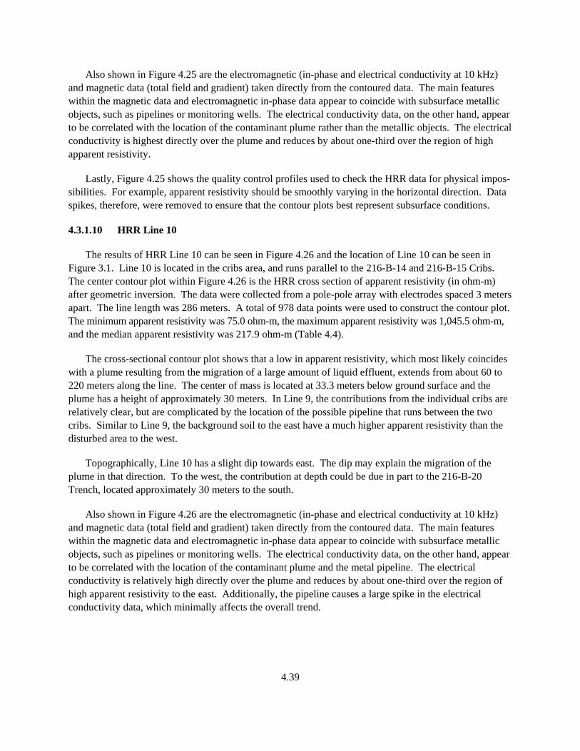
4.39
Also shown in Figure 4.25 are the electromagnetic (in-phase and electrical conductivity at 10 kHz) and magnetic data (total field and gradient) taken directly from the contoured data. The main features within the magnetic data and electromagnetic in-phase data appear to coincide with subsurface metallic objects, such as pipelines or monitoring wells. The electrical conductivity data, on the other hand, appear to be correlated with the location of the contaminant plume rather than the metallic objects. The electrical conductivity is highest directly over the plume and reduces by about one-third over the region of high apparent resistivity.
Lastly, Figure 4.25 shows the quality control profiles used to check the HRR data for physical impos-sibilities. For example, apparent resistivity should be smoothly varying in the horizontal direction. Data spikes, therefore, were removed to ensure that the contour plots best represent subsurface conditions.
4.3.1.10 HRR Line 10
The results of HRR Line 10 can be seen in Figure 4.26 and the location of Line 10 can be seen in Figure 3.1. Line 10 is located in the cribs area, and runs parallel to the 216-B-14 and 216-B-15 Cribs. The center contour plot within Figure 4.26 is the HRR cross section of apparent resistivity (in ohm-m) after geometric inversion. The data were collected from a pole-pole array with electrodes spaced 3 meters apart. The line length was 286 meters. A total of 978 data points were used to construct the contour plot. The minimum apparent resistivity was 75.0 ohm-m, the maximum apparent resistivity was 1,045.5 ohm-m, and the median apparent resistivity was 217.9 ohm-m (Table 4.4).
The cross-sectional contour plot shows that a low in apparent resistivity, which most likely coincides with a plume resulting from the migration of a large amount of liquid effluent, extends from about 60 to 220 meters along the line. The center of mass is located at 33.3 meters below ground surface and the plume has a height of approximately 30 meters. In Line 9, the contributions from the individual cribs are relatively clear, but are complicated by the location of the possible pipeline that runs between the two cribs. Similar to Line 9, the background soil to the east have a much higher apparent resistivity than the disturbed area to the west.
Topographically, Line 10 has a slight dip towards east. The dip may explain the migration of the plume in that direction. To the west, the contribution at depth could be due in part to the 216-B-20 Trench, located approximately 30 meters to the south.
Also shown in Figure 4.26 are the electromagnetic (in-phase and electrical conductivity at 10 kHz) and magnetic data (total field and gradient) taken directly from the contoured data. The main features within the magnetic data and electromagnetic in-phase data appear to coincide with subsurface metallic objects, such as pipelines or monitoring wells. The electrical conductivity data, on the other hand, appear to be correlated with the location of the contaminant plume and the metal pipeline. The electrical conductivity is relatively high directly over the plume and reduces by about one-third over the region of high apparent resistivity to the east. Additionally, the pipeline causes a large spike in the electrical conductivity data, which minimally affects the overall trend.
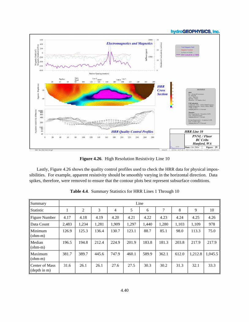
4.40
Figure 4.26. High Resolution Resistivity Line 10
Lastly, Figure 4.26 shows the quality control profiles used to check the HRR data for physical impos-sibilities. For example, apparent resistivity should be smoothly varying in the horizontal direction. Data spikes, therefore, were removed to ensure that the contour plots best represent subsurface conditions.
Table 4.4. Summary Statistics for HRR Lines 1 Through 10
Summary Line
Statistic 1 2 3 4 5 6 7 8 9 10
Figure Number 4.17 4.18 4.19 4.20 4.21 4.22 4.23 4.24 4.25 4.26
Data Count 2,483 1,234 1,281 1,909 1,297 1,440 1,280 1,103 1,109 978
Minimum (ohm-m)
126.9 125.3 136.4 130.7 123.1 88.7 85.1 98.0 113.3 75.0
Median (ohm-m)
196.5 194.8 212.4 224.9 201.9 183.8 181.3 203.8 217.9 217.9
Maximum (ohm-m)
381.7 389.7 445.6 747.9 460.1 589.9 362.1 612.0 1,212.8 1,045.5
Center of Mass (depth in m)
31.6 26.1 26.1 27.6 27.5 30.3 30.2 31.3 32.1 33.3
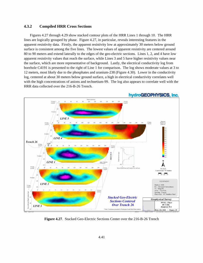
4.41
4.3.2 Compiled HRR Cross Sections
Figures 4.27 through 4.29 show stacked contour plots of the HRR Lines 1 through 10. The HRR lines are logically grouped by phase. Figure 4.27, in particular, reveals interesting features in the apparent resistivity data. Firstly, the apparent resistivity low at approximately 30 meters below ground surface is consistent among the five lines. The lowest values of apparent resistivity are centered around 80 to 90 meters and extend laterally to the edges of the geo-electric sections. Lines 1, 2, and 4 have low apparent resistivity values that reach the surface, while Lines 3 and 5 have higher resistivity values near the surface, which are more representative of background. Lastly, the electrical conductivity log from borehole C4191 is presented to the right of Line 1 for comparison. The log shows moderate values at 3 to 12 meters, most likely due to the phosphates and uranium-238 (Figure 4.30). Lower in the conductivity log, centered at about 30 meters below ground surface, a high in electrical conductivity correlates well with the high concentrations of anions and technetium-99. The log also appears to correlate well with the HRR data collected over the 216-B-26 Trench.
Figure 4.27. Stacked Geo-Electric Sections Center over the 216-B-26 Trench
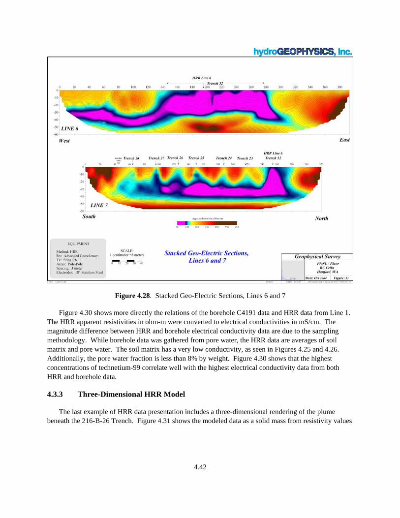
4.42
Figure 4.28. Stacked Geo-Electric Sections, Lines 6 and 7
Figure 4.30 shows more directly the relations of the borehole C4191 data and HRR data from Line 1. The HRR apparent resistivities in ohm-m were converted to electrical conductivities in mS/cm. The magnitude difference between HRR and borehole electrical conductivity data are due to the sampling methodology. While borehole data was gathered from pore water, the HRR data are averages of soil matrix and pore water. The soil matrix has a very low conductivity, as seen in Figures 4.25 and 4.26. Additionally, the pore water fraction is less than 8% by weight. Figure 4.30 shows that the highest concentrations of technetium-99 correlate well with the highest electrical conductivity data from both HRR and borehole data.
4.3.3 Three-Dimensional HRR Model
The last example of HRR data presentation includes a three-dimensional rendering of the plume beneath the 216-B-26 Trench. Figure 4.31 shows the modeled data as a solid mass from resistivity values
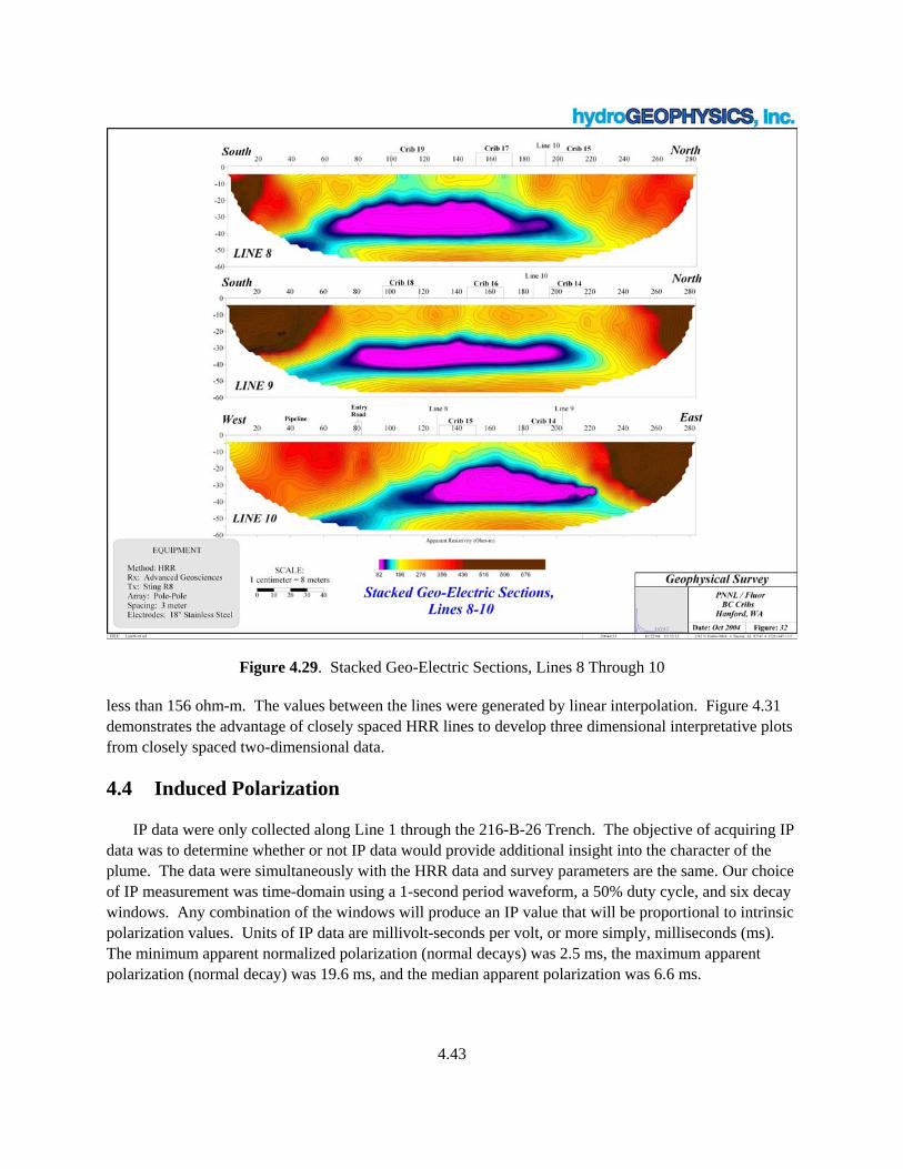
4.43
Figure 4.29. Stacked Geo-Electric Sections, Lines 8 Through 10
less than 156 ohm-m. The values between the lines were generated by linear interpolation. Figure 4.31 demonstrates the advantage of closely spaced HRR lines to develop three dimensional interpretative plots from closely spaced two-dimensional data.
4.4 Induced Polarization
IP data were only collected along Line 1 through the 216-B-26 Trench. The objective of acquiring IP data was to determine whether or not IP data would provide additional insight into the character of the plume. The data were simultaneously with the HRR data and survey parameters are the same. Our choice of IP measurement was time-domain using a 1-second period waveform, a 50% duty cycle, and six decay windows. Any combination of the windows will produce an IP value that will be proportional to intrinsic polarization values. Units of IP data are millivolt-seconds per volt, or more simply, milliseconds (ms). The minimum apparent normalized polarization (normal decays) was 2.5 ms, the maximum apparent polarization (normal decay) was 19.6 ms, and the median apparent polarization was 6.6 ms.
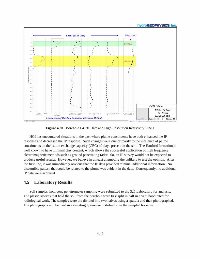
4.44
Figure 4.30. Borehole C4191 Data and High Resolution Resistivity Line 1
HGI has encountered situations in the past where plume constituents have both enhanced the IP response and decreased the IP response. Such changes were due primarily to the influence of plume constituents on the cation exchange capacity (CEC) of clays present in the soil. The Hanford formation is well known to have minimal clay content, which allows the successful application of high frequency electromagnetic methods such as ground penetrating radar. So, an IP survey would not be expected to produce useful results. However, we believe in at least attempting the unlikely to test the opinion. After the first line, it was immediately obvious that the IP data provided minimal additional information. No discernible pattern that could be related to the plume was evident in the data. Consequently, no additional IP data were acquired.
4.5 Laboratory Results
Soil samples from cone penetrometer sampling were submitted to the 325 Laboratory for analysis. The plastic sleeves that held the soil from the borehole were first split in half in a vent hood rated for radiological work. The samples were the divided into two halves using a spatula and then photographed. The photographs will be used in estimating grain-size distribution in the sampled horizons.
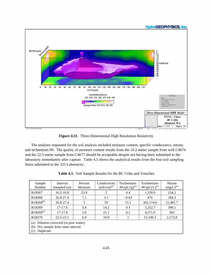
4.45
Figure 4.31. Three-Dimensional High Resolution Resistivity
The analytes requested for the soil analysis included moisture content, specific conductance, nitrate, and technetium-99. The quality of moisture content results from the 10.2-meter sample from well C4674 and the 22.5-meter sample from C4677 should be acceptable despite not having been submitted to the laboratory immediately after capture. Table 4.5 shows the analytical results from the four soil sampling liners submitted to the 325 Laboratory.
Table 4.5. Soil Sample Results for the BC Cribs and Trenches
Sample Number
Interval Sampled (m)
Percent Moisture
Conductivity (mS/cm)(a)
Technetium-99 (pCi/g)(a)
Technetium-99 (pCi/L)(a)
Nitrate (mg/L)(a)
B1BJ67 10.2-10.8 23.9 2 0.4 1,359.9 234.2 B1BJ68 26.8-27.4 7.1 3.1 <0.03 476 184.3 B1BJ68(b) 26.8-27.4 5 59 15.1 302,174.8 21,481.7 B1BJ69 17-17.6 3.4 14.2 0.1 3,252.7 390.1 B1BJ69(c) 17-17.6 3.0 15.1 0.1 4,271.9 362 B1BJ70 22.5-23.1 6.9 10.9 1 15,190.3 2,173.8 (a) Dilution corrected (in pore water). (b) Dry sample from same interval. (c) Duplicate.
4.46
The first boring located approximately 150 meters along Line 4 (Figure 4.20) is represented by the first three results. A split sample was recovered from the 26.8- to 27.4-meter interval due to an apparent dry zone near the base of the sample. The sample results indicate that significant moisture and technetium-99 can be found at a relatively shallow depth, and at some distance from the former trench boundary (approximately 3 meters). This indicates shallow, lateral spread of liquid effluent, or discharge outside of the trench boundary due to overflow. The second, deeper sample from 22.5 to 23.1 meters exhibited the highest activity of technetium-99 observed in this exercise. The concentration of nitrate was equally high, as was the specific conductance. These results were expected to correlate well, but the fact that moisture was low and the sample was visually dry is unexpected. Sample results for well C4677 have values that are more in line with the expected behavior for technetium-99 and nitrate. Both horizons had results that indicated a rise in technetium-99 and nitrate values with a rise in moisture.
5.1
5.0 Conclusions
Several surface geophysical methods were used to map subsurface features within the BC Cribs and Trenches Area. These methods included magnetic gradiometry, electromagnetic induction, HRR, and IP. The geophysical surveys were completed in four phases between the dates of July 11, 2004 and September 28, 2004.
The magnetic and electromagnetic data showed several localized anomalies that were unrelated to any natural geologic phenomena. In particular, large responses were seen in both total field and magnetic gradient near monitoring wells. These wells had casings that could be identified from the surface. Other features within the contour maps were not known with certainty, but were expected to be from abandoned pipeline networks that delivered liquid mixed waste from the 200 East Area to the north of the site. These pipelines formed linear features in the contour maps. One exception was with the electromagnetic induction in-phase data. Buried pipelines that were minimally coupled with the GEM-2 did not have a noticeable response in the data.
Overall, the ancillary reconnaissance magnetic and electromagnetic methods provided considerable insight to the study by clearly indicating (1) the presence of unknown pipelines (at least unknown to HGI); (2) the presence of magnetic and electrically conductive material in some trenches; (3) the presence of electrically conductive soil in areas not normally associated with planned waste disposal; and (4) the probable presence of basalt used for enhanced drainage. A specific goal for the electromagnetic survey was to delineate any shallow, electrically conductive soil that might interfere with the application or interpretation of the HRR survey. Of interest is the observation that there was no discernible shallow conductive material detected overlying the 216-B-26 Trench.
Ten lines of HRR data were gathered over the site, which were focused around the 216-B-26 and 216-B-52 Trenches and the 216-B-14 through 216-B-19 Cribs. The data showed that a large electrically conductive feature existed beneath all of the trenches and cribs sampled. This feature is extremely large, extending to depths of greater than 40 meters from the surface. The location of the feature correlates well with borehole geophysical and geochemical logs collected from the center of the 216-B-26 Trench. These logs showed that a high concentration of technetium-99, sulfates, nitrates, and chlorides existed at a depth centered at 30 meters below ground surface. Additionally, a high concentration of uranium-238 and phosphates were measured at depths from 3 to 12 meters.
The sample results from soil sampling activities confirm the relationship between technetium-99 activity and nitrate concentration. Apparent resistivity does not predict, however, the soil sampling results for a particular horizon. The relationship between the analytes selected for ground truth and the apparent resistivity measured from surface geophysics is complicated by the fact that resistivity analysis has a component of volume averaging that cannot discretely resolve horizons to the degree offered by soil sampling alone. The benefit that the resistivity surveys provide is a continuous profile of average conductivity in the subsurface that is difficult to reproduce solely by direct sampling in boreholes.
5.2
During the original discussions of geophysical methodologies, HGI’s RPM method was proposed as the culminating method to use once a plume had been identified. The objective of the RPM survey was to have better defined the plume shape and extent by electrically “lighting up” the plume. After completing the HRR phase of the site study, we realized that the extent of the plume was so great that the RPM method could not be deployed in the vicinity of the 216-B-26 Trench. The rationale behind the decision not to continue with RPM was the problem of the general absence of “native background” in the vicinity of the 216-B-26 Trench. The RPM method requires a substantial amount of background data in order to statistically discriminate the target. Such background was unavailable due to the considerable lateral extent of the plume. At present, HRR is a more cost-effective method for mapping the plume to the limits of detection. Any future efforts, however, to better define the distal portions and shape of the plume, i.e., the portions of the plume that cannot be easily mapped with surface-based HRR, will benefit by the use of RPM.
Lastly, the one proof-of-concept line of IP data collected at the site demonstrated that no charge storage mechanism was either created by the introduction of the liquid waste or was altered by the presence and/or passage of the liquid waste. Although some technical problems were encountered with the IP instrumentation, our conclusion is that there is no diagnostic IP signature associated with the liquid waste plume. Consequently, no IP data were acquired during the remainder of the HRR survey.
The presence of electrically conductive liquid waste (or its residue) in the electrically resistive vadose zone of the Hanford formation was confirmed and provided an excellent target. The depth-to-plume occurs well within the range of investigation of the HRR method allowing easy detection and excellent vertical and lateral definition.
6.1
6.0 Recommendations
As a preliminary study, this report shows that geophysical surveys can be used at the BC Cribs and Trenches Area for infrastructure and plume delineation. However, due to the extreme size of the plume, it is recommended that additional geophysical surveys be completed in order to fully understand the extent to which the technetium-99 plume has spread.
Suggestions for future geophysical mapping are as follows. Pacific Northwest National Laboratory and HGI are not aware of the extent of site-specific knowledge and that some recommendations may be unnecessary.
1. The principal tool of the study, HRR, can be used to map the entire BC Cribs and Trench Area site to delineate the existing plume. This can be done in a coarse coverage mode, from which three-dimensional models could not be created, but from which the general extent of the plume can be determined. Higher density coverage would allow the creation of three-dimensional models, such as that presented in this report, and provide higher definition of the plume site-wide.
2. The RPM method, untested during this study, may play a role in any future studies at the edge of the resolution provided by HRR surveying to extend the edge of the plume to areas where cumulative plume constituent concentrations are too low to be detected by a purely surficial method.
3. If any of the buried infrastructure (i.e., pipelines, valves, cribs, etc.) require better definition and/or quantifiable inverse modeling, then high-density magnetic and/or electromagnetic surveys may be performed. Such studies would require close-spaced data coverage and precision location. The end result would be geometric models that would define areas to either target by drilling, or to be avoided by drilling. Alternatively, infrastructure requiring removal for remediation and mitigation purposes can be satisfactorily located and mapped by localized precision surveys. All such surveys would be non-invasive.
4. Any future deployments of geophysical methods should include sufficient coverage over areas considered to represent native background. Such background data are necessary to correctly assess the degree or relevance of any anomalous features. As it presently stands, virtually the entire magnetic and electromagnetic surveys produce a background that we suspect is above native background. Comparison of anomalies to an elevated background diminishes the amplitude, and possibly the importance, of the anomalies.
5. Any subsequent drilling or cone penetrometer testing (CPT) should include electrical or induction logging and the installation of buried electrodes.
Difficulty in correlating data from the geophysical probe penetrometer to high resolution resistivity measurements is one task that should be overcome in future resistivity surveys. The need for proximity borehole data that can be used to more precisely locate vertical soil sampling locations warrants further testing. One possible avenue for resolving the differences in apparent resistivity models for the two

6.2
methods is to field both instruments in a strictly controlled test environment where variables affecting measurement can be controlled. Borehole technology that can produce predictive results for vertical soil sampling can complement both high resolution resistivity and soil sampling.
7.1
7.0 References
CERCLA – Comprehensive Environmental Response, Compensation, and Liability Act. 1980. Public Law 96-150, as amended, 94 Stat. 2767, 42 USC 9601 et seq.
Huang H and IJ Won. 2000. “Conductivity and Susceptibility Mapping Using Broadband Electromagnetic Sensors.” Journal of Environmental and Engineering Geophysics 5(4):31-41.
Lindsey KA. 1991. Revised Stratigraphy for the Ringold Formation, Hanford Site, South-Central Washington. WHC-SD-EN-EE-004, Westinghouse Hanford Company, Richland, Washington.
Lindsey KA, SP Reidel, KR Fecht, JL Slate, AG Law and AM Tallman. 1994. “Geohydrologic Setting of the Hanford Site, South-Central Washington.” In Geologic Field Trips in the Pacific Northwest, 1994 Annual Meeting, DA Swanson and RA Haugerud (eds.), Geological Society of America 1:1C-1-16.
RCRA – Resource Conservation and Recovery Act. 1976. Public Law 94-580, as amended, 90 Stat. 2795, 42 USC 6901 et seq.
Reidel SP. 2004. Geologic Data Package for 2005 Integrated Disposal Waste Performance Assessment. PNNL-14586, Pacific Northwest National Laboratory, Richland, Washington.
Serne RJ and FM Mann. 2004. Preliminary Data from 216-B-26 Borehole in BC Cribs. RPP-20303, Rev. 0, CH2M HILL Hanford Group, Inc., Richland, Washington.
Tallman AM, KR Fecht, MC Marratt, and GV Last. 1979. Geology of the Separations Areas, Hanford Site, South-Central Washington. RHO-ST-23, Rockwell Hanford Operations, Richland, Washington.
Telford WM, LP Geldart, and RE Sheriff. 1990. Applied Geophysics. Cambridge University Press, Cambridge, United Kingdom.
U.S. Department of Energy (DOE). 1988. Consultation Draft Site Characterization Plan. Reference Repository Location, Hanford Site Washington. DOE/RW-0164, U.S. Department of Energy, Office of Civilian Waste Management, Washington D.C.
U.S. Department of Energy (DOE). 1992. B Plant Source Aggregate Area Management Study Report. DOE/RL-92-05, Draft A., U.S. Department of Energy, Richland Operations Office, Richland, Washington.
U.S. Department of Energy (DOE). 2000. 200-TW-1 Scavenged Waste Group Operable Unit and 200-TW-2 Tank Waste Operable Unit RI/FS Workplan. DOE/RL-2000-38, Draft A, U.S. Department of Energy, Richland Operations Office, Richland, Washington.

7.2
U.S. Department of Energy (DOE). 2003. Sampling and Analysis Plan for the BC Cribs and Trenches Area. DOE/RL-2003-44, Draft A, U.S. Department of Energy, Richland Operations Office, Richland, Washington.

Appendix
Soil Sample Core Photographs from Wells C4674 and C4677
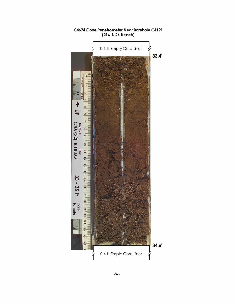
A.1
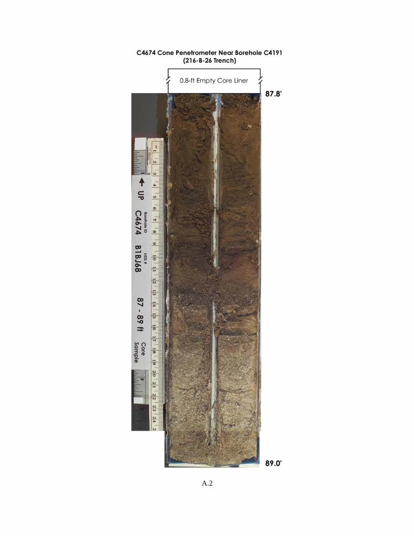
A.2
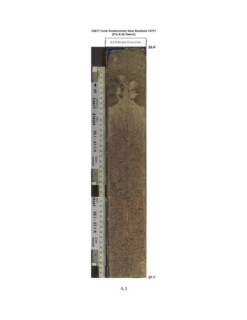
A.3
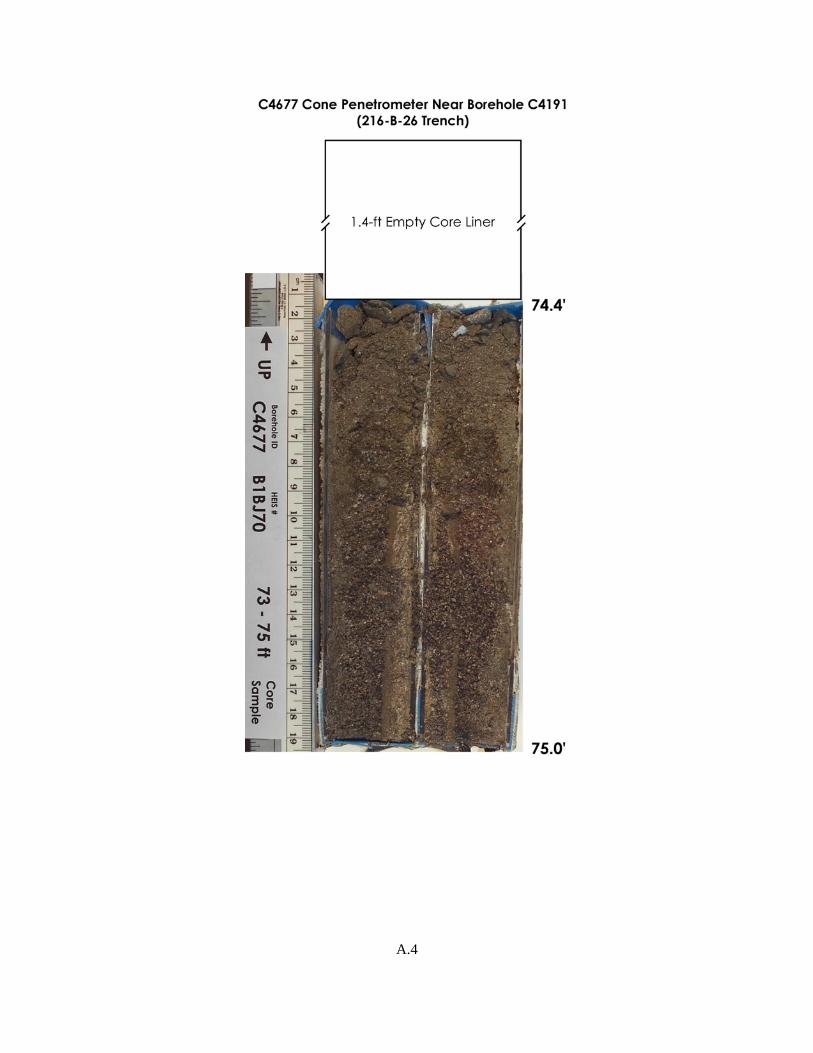
A.4
PNNL-14948
Distr.1
Distribution No. of Copies OFFSITE 3 Dale Rucker hydroGEOPHYSICS, Inc. 2302 N. Forbes Boulevard Tucson, Arizona 85745 ONSITE 6 Fluor Hanford, Inc. M. W. Benecke E6-35
No. of Copies 11 Pacific Northwest National Laboratory D. B. Barnett K6-81 M. D. Freshley K9-33 G. W. Gee K9-33 C. T. Kincaid K9-33 M. D. Sweeney (4) K6-81 A. L. Ward K9-33 Hanford Technical Library (2) P8-55