PLEASE DO NOT USE, COPY OR DISTRIBUTE WITHOUT THE AUTHOR’S PERMISSION 1 2002-10-29 BU CAS CS-350...

PLEASE DO N

OT USE, C

OPY OR D

ISTRIBUTE WITHOUT THE AUTHOR’S PERMISSIO

N

12002-10-29

BU CAS CS-350Fundamentals of Computer

Systems

Fall 2002Prof. Abdelsalam ‘Solom’ Heddaya

www.cs.bu.edu/fac/heddaya/course/cs350

This is a Hypertext DocumentClick on Icons and Links to View in Full

PLEASE DO N

OT USE, C

OPY OR D


N

22002-10-29

Course Intro

PLEASE DO N

OT USE, C

OPY OR D


N

32002-10-29

Today’s Agenda

• People– Instructor, TF, students

• Resources– Web site

– Mailing list

• Course description and role– Solving practical system problems using maths

• Course organization and policies

• Next class: review of computer system organization

PLEASE DO N

OT USE, C

OPY OR D


N

42002-10-29

People

• Instructor: Abdelsalam ‘Solom’ Heddaya– Chief Technology Officer and co-founder of InfoLibria, Inc. (

www.infolibria.com)

– Adjunct Associate Professor, BU CS Dept.

– Nine years as full-time professor, and five years as entrepreneur

– Helped conceive cs350 as a new unique course in 1996/97

• Teaching fellow: Gali Diamant– Ph.D. student

– Additional info soon

• Students…

PLEASE DO N

OT USE, C

OPY OR D


N

62002-10-29

Resources

• Web site– www.cs.bu.edu/fac/heddaya/course/cs350

• Mailing list– Will be used for last-minute announcements (e.g., homework corrections)

– [email protected]

– Join by following instructions

• Office hours– Prof. Heddaya: TR 3:30-4:00pm, or by appointment

– Gali Diamant: TBA

• Grades– Will be posted regularly on the web site, under a secret ID that you will

choose as part of homework #1

PLEASE DO N

OT USE, C

OPY OR D


N

72002-10-29

CS-350 in a Nutshell

• About– Modeling systems, so as to think about them

– Thinking about systems helps us understand existing ones, and design new ones

– Focus on most difficult problems•Performance: how to keep key resources busy and responding quickly

•Concurrency: how to keep track of many things happening at once

• NOT about– Programming

– Theory

PLEASE DO N

OT USE, C

OPY OR D


N

82002-10-29

Role of CS-350(See CS Course Map)

• CS-350 builds on– Computer systems organization (CS-210)

– Algorithms and data structures (CS-112)

– Discrete Maths (MA-293)

• CS-350 prepares for– Performance Analysis (CS-470)

– Operating Systems (CS-552)

– Databases (CS-560)

– Networking (CS-555/556)

– Architecture (CS-450/550)

• Jobs in which these skills come in handy– System designer, architect, CTO, etc.

– Researcher, academic, consultant

– Software developer, product manager, performance engineer, etc.

– Market analyst, journalist, etc.

• Where does CS-350 fit in “The Big Picture™”?

PLEASE DO N

OT USE, C

OPY OR D


N

102002-10-29

Organization of CS-350

• Review of course syllabus– www.cs.bu.edu/fac/heddaya/course/cs350

PLEASE DO N

OT USE, C

OPY OR D


N

122002-10-29

Extra Stuff

PLEASE DO N

OT USE, C

OPY OR D


N

132002-10-29

A Flavor of CS-350

• System– A collection of interacting parts, together with,

– A demarcation between system and its environment (an interface)•Typically represents a narrow interface, but,

•Arbitrary nonetheless

• System quality metrics (looking from the outside)– Safe, secure

– Available, reliable

– Fast•Throughput (work done per second)

•Response time (time required to finish one task)

– Efficient (consumes minimal resources)

• System quality metrics (looking inside)– Cheap to build

– Cheap to maintain

– Elegant

PLEASE DO N

OT USE, C

OPY OR D


N

142002-10-29

Where does the System End and “I” Start?

• Machine is obedient slave to its human master

• An alternative model– Isaac Asimov’s Three Laws of Robotics (see “I, Robot”, a collection of

short stories written in the 1940s and 50s and still in print)1. A robot may not injure a human being, or, through inaction, allow a human

being to come to harm.

2. A robot must obey the orders given it by human beings, except where such orders would conflict with the First Law.

3. A robot must protect its own existence, except where such protection would conflict with the First or Second Law.

• Shouldn’t the human be considered part of the “system”?– Important in designing safe systems, because

– Enables accounting of human error as a sub-system failure to be handled by overall system

– Also, allows for accounting for human response times as part of overall system performance

PLEASE DO N

OT USE, C

OPY OR D


N

152002-10-29

Hurry Up and Wait:

Modeling Queues

PLEASE DO N

OT USE, C

OPY OR D


N

162002-10-29

Today’s Agenda

• Administrivia

1. A simple model: the queue1. Discover: throughput, response time and waiting capacity

2. Laws:1. Flow Conservation

2. Little’s Law

PLEASE DO N

OT USE, C

OPY OR D


N

172002-10-29

Administrivia

• Web site

• Mailing list

• Policies– Please read; will be frozen next Friday

– Email me comments on policy NOW

• Section schedule change:– Instead of 3 sections, we can only have two

– Proposed time slots—any two of:•Mon

– 11-12 (current)

– 3-4

•Fri– 12-1

– 2-3 (current)

– 3-4 (current)

PLEASE DO N

OT USE, C

OPY OR D


N

182002-10-29

Modeling with Queues

• Simple

• Widely applicable to quantitative aspects of system performance

• Susceptible to easy, back-of-the-envelope analysis– Yet, extremely robust results that are widely applicable

• Can also be analyzed probabilistically– More difficult later in course

– Yields more detailed information (probability distributions, not just averages)

– Less robust results (depends on somewhat fragile assumptions)

PLEASE DO N

OT USE, C

OPY OR D


N

192002-10-29

Single Queue

• Tasks arrive at an average rate = • Tasks wait in the queue until it is their return

– Doesn’t matter how turn is determined

– Average number of tasks waiting = w

– Average number of tasks waiting and being serviced = q

• Server performs the work required by the task, at an average = – Server is not busy all the time

– Average fraction of time server is busy =

• Tasks depart, after being serviced, at an average rate = ?– When server is busy, average departure rate = ?

– When server is idle, average departure rate = ?

Queue Server

Task

Arrivals atmean rate =

Service rate =

System

Departures at

mean rate = .

PLEASE DO N

OT USE, C

OPY OR D


N

212002-10-29

Flow Conservation Law

• Flow-conservation law– Over a sufficiently long period of time, we must have

Mean departure rate = Mean arrival rate =, and

Mean departure rate Mean service rate =

Queue Server


Service rate =

Departures at mean

rate = . =

PLEASE DO N

OT USE, C

OPY OR D


N

232002-10-29

Little’s Law

•Glossary– Mean arrival rate = – Mean service rate = – Mean number of tasks in queue = w

– Mean response time = tq

•Little’s law

1

qtq

Queue Server


Service rate =

Departures at

mean rate =

PLEASE DO N

OT USE, C

OPY OR D


N

242002-10-29

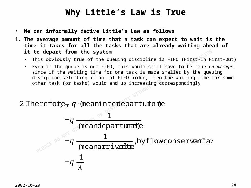
Why Little’s Law is True

• We can informally derive Little’s Law as follows

1. The average amount of time that a task can expect to wait is the time it takes for all the tasks that are already waiting ahead of it to depart from the system• This obviously true of the queuing discipline is FIFO (First-In First-Out)

• Even if the queue is not FIFO, this would still have to be true on average, since if the waiting time for one task is made smaller by the queuing discipline selecting it out of FIFO order, then the waiting time for some other task (or tasks) would end up increasing correspondingly

1

lawon conservati-flowby , )rate arrivalmean (

1

)rate departuremean (

1

) timedeparture-intermean ( Therefore, 2.

q

q

q

qtq

PLEASE DO N

OT USE, C

OPY OR D


N

252002-10-29

New Lecture

PLEASE DO N

OT USE, C

OPY OR D


N

262002-10-29

Today’s Agenda

• Administrivia– HW 1 out: electronic hand-in tentative until confirmed by email

1. Computer Organization—a review1. Core hardware

2. Processor-memory-I/O interactions

2. Improving CPU utilization (efficiency)1. Using interrupts

2. Using memory caching (probably next class)

• Next class: from program to process

PLEASE DO N

OT USE, C

OPY OR D


N

272002-10-29

The Core Hardware

PSR = Program Status Register

PSRSimplified model• Works only for single

straight-line program

What’s missing?• Subroutine support

• I/O management

• Memory management

• Multi-tasking support

PLEASE DO N

OT USE, C

OPY OR D


N

282002-10-29

The Basic Instruction Cycle

1. CPU fetches the next instruction (with operands) from memory

2. Program Counter (PC) incremented• To point to subsequent instruction in memory (assumes sequential program)

3. CPU executes the instruction• Instruction applied to operands stored in registers (after possibly having been

fetched from memory in step 1)

• Instruction may be conditioned on the value of certain bits in Program Status Register (PSR)

• The instruction may modify the Program counter (PC), so as to cause the CPU to execute an instruction that is out-of-sequence

PLEASE DO N

OT USE, C

OPY OR D


N

292002-10-29

Basic Control & Status Registers

• Program Counter (PC)– Contains the address of the next instruction

to be fetched

• Instruction Register (IR)– Contains the instruction most recently

fetched

• Program Status Register (PSR)– condition codes and status info bits– Interrupt enable/disable bit– Supervisor(OS)/user mode bit

• Data Registers– Store instruction operands and results– Can be copied from/to memory locations

• Address Registers– Contain memory address of data and

instructions– May contain a portion of an address that is

used to calculate the complete address

PLEASE DO N

OT USE, C

OPY OR D


N

302002-10-29

Memory Addressing Modes

• Direct– MAR gives the absolute physical memory address of the desired item

• Indirect– MAR contains the absolute address of a memory location that contains

the absolute address of the desired item

• Indexed– MAR provides an index value to be added to a base value to get the

absolute memory address

• Segment pointer– When address space is divided into segments, memory is referenced by a

segment number and an offset in that segment

• Stack pointer– Points to top of stack

– Instruction or register provides an offset (usually small)

– For subroutine entry/exit (Appendix 1B)

PLEASE DO N

OT USE, C

OPY OR D


N

312002-10-29

Must CPU Wait for I/O to Complete?

Example• WRITE transfers control to the

printer driver (I/O pgm)

• I/O pgm prepares I/O module for printing (4)

• CPU has to WAIT for I/O command to complete

• I/O pgm finishes and reports status of operation

• CPU wastes much time waiting

PLEASE DO N

OT USE, C

OPY OR D


N

322002-10-29

Interrupts

• Invented to allow overlap of input and processing times

• CPU launches I/O, returns to processing and then gets interrupted when I/O completed

• The I/O module sends an interrupt request– Via a direct connection, or via a control bus

• Then CPU transfers control to an Interrupt Handler Routine (normally part of the OS)

PLEASE DO N

OT USE, C

OPY OR D


N

332002-10-29

User program must restart as if there was no interruption

Interrupt Handling

• Similar to subroutine call but not controlled by user program

PLEASE DO N

OT USE, C

OPY OR D


N

342002-10-29

Instruction Cycle with Interrupts

• If interrupts are enabled, CPU checks for interrupts after each instruction

• If no interrupts, then fetch the next instruction for the current program

• If an interrupt is pending, then suspend execution of the current program, and execute the interrupt handler (in the OS)

• Note: – Disabling interrupts should be done only when really necessary, because it can

cause loss of information.

PLEASE DO N

OT USE, C

OPY OR D


N

352002-10-29

Interrupt Handler

• Is a program that determines nature of the interrupt and performs whatever actions are needed

• Upon interrupt, control is transferred to this program – This is done by transferring control to a memory location that is

determined by the type of interruption, according to an interrupt vector (table)

– Control must be transferred back to the interrupted program so that it can be resumed from the point of interruption

• The point of interruption can be anywhere in the program (except where interrupt explicitly inhibited)

• Thus– Must save the state of the process (content of PC + PSW + registers + ...)

– Where can this be done?

PLEASE DO N

OT USE, C

OPY OR D


N

362002-10-29

Interrupts improve CPU usage

• I/O pgm prepares the I/O module and issues the I/O command (eg, to printer)

• Control returns to user pgm

• User code gets executed during I/O operation: no waiting

• User pgm gets interrupted (x) when I/O operation is done

• Control goes to interrupt handler to check status of I/O module and perform necessary processing

• Execution of user code resumes

PLEASE DO N

OT USE, C

OPY OR D


N

372002-10-29

Types of Interrupts

• Not normalized, but it is a good idea to distinguish between:– traps or exceptions: caused by the pgm as it executes

•division by 0

•illegal access

•system calls...

– interruptions: caused by independent events:•end I/O

•timers

– faults: term used esp. in connection with paging and segmentation

• But the hardware mechanisms are similar for all

PLEASE DO N

OT USE, C

OPY OR D


N

382002-10-29

Multiple interrupts: sequential order

• Disable interrupts during an interrupt

• Interrupts remain pending until the processor enables interrupts

• After interrupt handler routine completes, the processor checks for additional interrupts

PLEASE DO N

OT USE, C

OPY OR D


N

392002-10-29

Multiple Interrupts: priorities

• Higher priority interrupts cause lower-priority interrupts to wait

• Causes a lower-priority interrupt handler to be interrupted

• Example– When input arrives from communication line, it needs to be absorbed quickly to

avoid retransmission

• This requires a stack mechanism to save registers, etc.

PLEASE DO N

OT USE, C

OPY OR D


N

402002-10-29

Long I/O

• Normally I/O is very long with respect to I/O processing

• In this case, the program and the CPU will have to wait even if there is concurrency between I/O and CPU processing

PLEASE DO N

OT USE, C

OPY OR D


N

412002-10-29

Extra Stuff

PLEASE DO N

OT USE, C

OPY OR D


N

422002-10-29

Multiprogramming

• Allows better use of I/O overlap times

• When a program reads a value on an I/O device it may wait long time for the I/O operation to complete

– It can be difficult to use this waiting time

• So interrupts are mostly effective when a single CPU is shared among several concurrently active processes

• The CPU can then switch to execute another program when a program waits for the result of the read operation

PLEASE DO N

OT USE, C

OPY OR D


N

432002-10-29

Memory Hierarchy

PLEASE DO N

OT USE, C

OPY OR D


N

442002-10-29

Cache Memory

• Small fast cache– Interacting with slower but much

larger memory

• Transparent (invisible) to OS and user programs

– But interacts with other memory management hardware

• Processor first checks– If word referenced is in cache

• If not found in cache– A block of main memory containing

the word is moved to the cache

PLEASE DO N

OT USE, C

OPY OR D


N

452002-10-29

The Hit Ratio

• Hit ratio =– Fraction of access where data is in

cache

• T1 =– Access time for fast memory

• T2 =– Access time for slow memory

• T2 >> T1

• Vertical axis = – Average access time

• When hit ratio is close to 1– Average access time is close to T1

PLEASE DO N

OT USE, C

OPY OR D


N

462002-10-29

Locality of Reference

• Memory references for both instruction and data tend to cluster over a long period of time

• Example– Once a loop is entered, there is frequent access to a small set of

instructions

– Similarly, data is usually accessed in sequence

• Hence– Once a word gets referenced, it is likely that nearby words will get

referenced often in the near future

• Thus, the hit ratio will be close to 1 even for a small cache

PLEASE DO N

OT USE, C

OPY OR D


N

472002-10-29

Disk Cache (Same Idea)

• A portion of main memory used to temporarily hold data from/to disk

• Locality of reference also applies here– Once a record (or portion of a file) gets referenced, it is likely that nearby

records will get referenced often in the near future

• If a record referenced is not in the disk cache, the block containing the record is moved into the disk cache

PLEASE DO N

OT USE, C

OPY OR D


N

482002-10-29

New Lecture

PLEASE DO N

OT USE, C

OPY OR D


N

492002-10-29

Today’s Agenda

• Administrivia

1. From program to process

2. Process states and transitions (basic model)

3. Swapping processes out of memory improves memory utilization

• Next class– My system is better than yours: system quality attributes

PLEASE DO N

OT USE, C

OPY OR D


N

502002-10-29

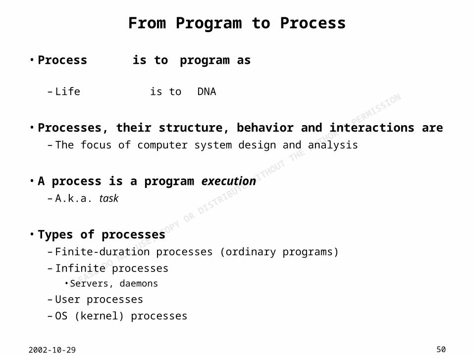
From Program to Process

• Process is to program as

– Life is to DNA

• Processes, their structure, behavior and interactions are– The focus of computer system design and analysis

• A process is a program execution– A.k.a. task

• Types of processes– Finite-duration processes (ordinary programs)

– Infinite processes•Servers, daemons

– User processes

– OS (kernel) processes

PLEASE DO N

OT USE, C

OPY OR D


N

512002-10-29

When Does a Process Get Created?

• Submission of a job

• User logs on

• Created by OS to provide a service to a user– Examples: printing

• Spawned by an existing process– A user program can dictate the creation of a number of processes

PLEASE DO N

OT USE, C

OPY OR D


N

522002-10-29

When Does a Process Get Terminated?

• User logs off

• Process executes a system call to terminate

• Error or fault conditions, timeout

PLEASE DO N

OT USE, C

OPY OR D


N

532002-10-29

There Can Be Many Processes

• Many processes tend to run “simultaneously”, even on uni-processor machines

• Multiple processes could be created from the same program

PLEASE DO N

OT USE, C

OPY OR D


N

542002-10-29

How a Process is Created

1. Program R memory image (binary) is stored in a file– Result of compilation

2. Another process asks the OS kernel to execute R• Via a special system call (exec in Unix)

3. Kernel allocates memory for a new process P• Can be physical or virtual memory

4. Kernel creates Process Control Block (PCB) for P• Holds information about P, including

• State (for scheduling purposes)

• Identity (for security purposes)

• Resources (for resource management purposes)

5. Kernel copies R from file to memory of process P

6. Kernel transfers control to the first instruction in P

PLEASE DO N

OT USE, C

OPY OR D


N

552002-10-29

Issues in Process Creation

1. How does the executable program R get created in the first place?1. What if R belongs to an interpreted language?

• Such as PERL, Java, Lisp, etc.

2. What if R doesn’t contain all the code necessary for P?• Typical case; otherwise executables would have to include the huge

libraries that they need to run

3. What if R can only run correctly if it runs in isolation?• For example, R is a real-time program that controls a life-critical device

4. What if N processes are created from the same program R?• Should they consume N times the memory?

5. Is it useful to group processes, so that a single program execution could create multiple communicating processes?

6. What is the cost of allowing the proliferation of processes?1. Are there light-weight processes with low “overhead”?

• For answers, take CS-552 Operating Systems– Prof. Rich West

PLEASE DO N

OT USE, C

OPY OR D


N

562002-10-29

Process States

• Running state– The process that is executing on the CPU is in Running state

• Blocked state– A process that is waiting for something (e.g., I/O) to complete is in

Blocked state

• Ready state– A process that is ready to be executed is in Ready state (due to limited

number of CPUs)

PLEASE DO N

OT USE, C

OPY OR D


N

572002-10-29

Other Useful States

• New state– OS has performed the necessary actions to create the process

•Has created a process identifier

•Has created tables needed to manage the process

– But, has not yet committed to execute the process (not yet admitted)• Because resources are limited

– Long-term scheduler takes this admission control decision

• Exit state– Termination moves the process to this state

– It is no longer eligible for execution

– Tables and other info are temporarily preserved for auxiliary program•E.g., accounting program that cumulates resource usage for billing the users

– The process (and its tables) gets deleted when the data is no longer needed

PLEASE DO N

OT USE, C

OPY OR D


N

582002-10-29

A Five-state Process Model

PLEASE DO N

OT USE, C

OPY OR D


N

592002-10-29

Process State Transitions [1/4]

• New Ready (a.k.a admit)– Long-term scheduler decides that the process can be executed

PLEASE DO N

OT USE, C

OPY OR D


N

602002-10-29


• Ready Running– The scheduler selects a new process to run (discussed later in course)

• Running Ready– The running process is timed out

– The running process gets interrupted because a higher priority process is in the ready state (needs to run)

• Or because compute-hungry process exhausted its fair share of CPU

PLEASE DO N

OT USE, C

OPY OR D


N

612002-10-29


• Running Blocked– When a process requests something for which it must wait

• A service of the OS that requires a wait

• An access to a resource not yet available

• Initiates I/O and must wait for the result

• Waiting for a process to provide input (IPC)

• Blocked Ready– When the event for which it was waiting occurs

PLEASE DO N

OT USE, C

OPY OR D


N

622002-10-29


• Running Exit– Process executes system call to exit

– Process killed by some external action (user, parent, OS)

PLEASE DO N

OT USE, C

OPY OR D


N

632002-10-29

A Queuing Model

• Queue Ready: processes waiting to get executed on CPU

• When event n occurs, the process that was waiting for it is moved into the Ready queue

PLEASE DO N

OT USE, C

OPY OR D


N

642002-10-29

Variations on the Basic Model

• The basic model we have discussed is very widely used

• It has a great number of variations, since no two OS’s are alike

• An example follows– Adding swapping states

PLEASE DO N

OT USE, C

OPY OR D


N

652002-10-29

Swapping Improves Memory Utilization

• So far, all the processes had to be (at least partly) in main memory

• Even with virtual memory, keeping too many processes in main memory will deteriorate the system’s performance

– E.g., coexistence of several processes that do not use CPU much

• The OS may need to suspend some processes to bring in others

– That is, to swap them out to auxiliary memory (disk)

• We add 2 new states, which double Blocked and Ready: – Blocked Suspend

•Blocked processes which have been swapped out to disk

– Ready Suspend•Ready processes which have been swapped out to disk

PLEASE DO N

OT USE, C

OPY OR D


N

662002-10-29

A Seven-state Process Model

PLEASE DO N

OT USE, C

OPY OR D


N

672002-10-29

New State Transitions

• Blocked Blocked Suspend– When all processes are blocked, the OS may remove a blocked process to

bring a ready process in memory

• Blocked Suspend Ready Suspend– When the event for which process has been waiting occurs

• Ready Suspend Ready– When no ready processes in main memory

– Normally, this transition is paired with Blocked --> Blocked suspend for another process (memory space must be found)

• Ready Ready Suspend– When there are no blocked processes and must free memory for

adequate performance

PLEASE DO N

OT USE, C

OPY OR D


N

682002-10-29

New Lecture

PLEASE DO N

OT USE, C

OPY OR D


N

692002-10-29

Today’s Agenda

• Administrivia

1. System quality attributes1. As black box

2. As white box

2. System quality metrics1. Measurable, objective, and quantifiable

3. System quality determination1. Modeling

1. Analysis

2. Simulation

2. Measurement

• Next time: intro to probability

PLEASE DO N

OT USE, C

OPY OR D


N

702002-10-29

What is a “System”?

• What is the difference between a system and a pile of components?

– A jumble of lines of code vs. an OS kernel

• System– A collection of interacting parts, together with,– A demarcation between system and its environment (an interface)

•Typically represents a narrow interface

– Each part is itself a system (whose internals we don’t care about)

• System environment– Everything that is not inside the system, including human users and other

systems

• System behavior (a.k.a. functionality)– Interactions with its environment– What happens inside the system is not behavior

• System correctness– System’s behavior falls within specification (or at least expectation)

• System failure– System violates its specified (or expected) behavior

PLEASE DO N

OT USE, C

OPY OR D


N

712002-10-29

System Quality Attributes

• System as a black box (looking from outside)– Safe, secure, private

– Available, reliable

– Fast•Throughput (work done per second)

•Response time (time required to finish one task)

– Efficient (overhead consumes minimal resources)•Scalable (performance improves with added resources)

– Domain of cs-350

• System as a white box (looking inside)– Easy to build (i.e., cheap to develop)

– Easy to maintain (i.e., cheap to own and to improve)

– Elegant, beautiful (i.e., pleasing to build and maintain)

– Domain of software engineering

PLEASE DO N

OT USE, C

OPY OR D


N

722002-10-29

System Quality Metrics [1/4]

Attribute

Metric Definition

Safe Safety System behavior never harms its environment, even when it fails.

Examples:

1. Application executes an illegal instruction or references protected memory

Secure,Private

Immunity against attack (a.k.a. security)

Each type of attack yields a different definition.

Examples of attacks:

1. Eavesdropping: attacker obtains fully-detailed copy of victim’s information

2. Spoofing: attacker tricks victim into accepting information as from a particular source

3. Denial-of-service: attacker prevents victim from offering or receiving service

4. Timing: attacker detects activity by victim (weaker form of eavesdropping)

PLEASE DO N

OT USE, C

OPY OR D


N

732002-10-29


Attribute

Metric Definition

Available Availability Fraction of time system is up (i.e., can accept requests for service)

•Typically expressed in percentage (e.g., 99.999%)

•Better expressed as (1-10-A), i.e., as the “number of 9’s”

•More important for short-duration services (what should the availability of the email server be?)

Reliable Reliability Length of time system is up (i.e., can sustain a long-running activity)

•Mean Time between Failures (MTBF) is a common statistic for this metric

•More important for long-duration services (what should the MTBF of a space probe be?)

•Availability = MTBF/(MTBF+MTTR)

PLEASE DO N

OT USE, C

OPY OR D


N

742002-10-29


Attribute

Metric Definition

Fast Throughput Number of units of work completed per unit time

Examples

1. A CPU capable of 2,000 MIPS

2. A disk capable of 140 MBps (MB/s)

3. A web server capable of 2,000 OPS

4. A network link capable of 2.5 Gbps (Gb/s)

Response time

Length of time a unit of work remains in the system before it is completed

Examples

1. A disk drive that completes an I/O in 11 milliseconds

2. A web server that completes an operation in 20 milliseconds

3. A network that can transmit a packet in 80 milliseconds from Boston to San Francisco

PLEASE DO N

OT USE, C

OPY OR D


N

752002-10-29


Attribute

Metric Definition

Efficient Utilization(a.k.a. efficiency)

Fraction of time a resource is busy (doing useful work)

Alternatively: fraction of theoretical peak capacity that can be utilized

Examples

1. An OS that can keep the CPU busy 80% of the time

2. A file system that can keep the disk busy 70% of the time)

3. A communication protocol that can run a network link at 50% of capacity

Scalability Utilization as a function of peak theoretical capacity (amount of resources)

Examples

1. A database server that can utilize one node at 80%, two nodes at 75%, three nodes at 70%

PLEASE DO N

OT USE, C

OPY OR D


N

762002-10-29

System Modeling Big Picture

System Model

Resources

Workload Metric =

f(workload, resources)

PLEASE DO N

OT USE, C

OPY OR D


N

772002-10-29

System Quality Determination

• Modeling1. Analysis (requires model to be mathematically tractable)

• Analyze for the functional forms of the relevant metrics, as functions of amount of resources and of load characteristics

• Compute (by software) the value of relevant metrics numerically– Can generate functional forms in the form of tables

2. Simulation• Measure the value of relevant metrics, by running the model and

then directly measuring the metrics• May use synthetic or real workloads to drive the simulation

• Requires model to be effective and efficient, such that experimenting with the simulator is faster, better and cheaper than with the system itself

• Measurement (requires some modeling)1. In vitro (in the lab, under synthetic or real workload)

2. In vivo (in the field, under real workload)

PLEASE DO N

OT USE, C

OPY OR D


N

782002-10-29

New Lecture

PLEASE DO N

OT USE, C

OPY OR D


N

792002-10-29

Today’s Agenda

• Administrivia– Readings (by A. Bestavros) available via web site (UID and password

sent by email)

1. Probability1. What is it? What can it model?

2. An example: what is the probability that two people have the same birthday, in a class of N students?

2. Definitions

3. Composing events1. A or B (a.k.a. union, disjoint)

2. A and B (a.k.a. intersection, joint)

3. A given B (a.k.a. conditional)

4. Random variables

5. Distributions

• Next time: More probability

PLEASE DO N

OT USE, C

OPY OR D


N

802002-10-29

Probability—What is it?

• A mathematical construction– Can be studied in total isolation of the real world

• Models uncertainty (ignorance), as well as randomness

• Useful primarily for large populations (the larger the better), or long histories (the longer the better)

– What happens if you use probability modeling and analysis to gamble?

• Strongly related to counting

PLEASE DO N

OT USE, C

OPY OR D


N

812002-10-29

Example—Probability of Same-day Birthdays

• Given a class with N students in it, what is the probability that two students have the same birthday?

– The answer, for N = 29, may surprise you•Odds?

– The answer for N = 367, should not surprise you

• Approach– Solve for N = 2

– Count the total number of possible birthday lists

– Count the number of possible birthday lists with two or more identical birthdays (call these lists the birthday coincidence, or BC, lists)

– Assume that every one of the birthday lists is equally likely

– Find the frequency of the event that a list is a BC list

PLEASE DO N

OT USE, C

OPY OR D


N

822002-10-29

Same-day Birthdays

• N = 2– Answer = 1/365 (why?)

• Total number of possible birthday lists= 365N

• Number of possible birthday lists with two or more (up to N) repetition

= total – number of birthday lists with no repetition

= 365N - 365 x 364 x 363 x … x (365-N+1)

= 365N - 365! / (365-N)!

• Assume that every one of the birthday lists is equally likely– That is, we assume that there is no self-selection

– Is this assumption true?

• Probability that two (or more) people out of N have the same birthday

= [365N - 365! / (365-N)! ] / 365N

PLEASE DO N

OT USE, C

OPY OR D


N

842002-10-29

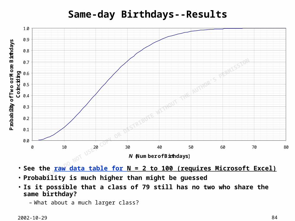
Same-day Birthdays--Results

• See the raw data table for N = 2 to 100 (requires Microsoft Excel)• Probability is much higher than might be guessed• Is it possible that a class of 79 still has no two who share the same

birthday?– What about a much larger class?

0.0

0.1

0.2

0.3

0.4

0.5

0.6

0.7

0.8

0.9

1.0

0 10 20 30 40 50 60 70 80

N (Number of Birthdays)

Pro

bab

ilit

y o

f T

wo

or

Mo

re B

irth

day

s C

oin

cid

ing

PLEASE DO N

OT USE, C

OPY OR D


N

852002-10-29

Key Definitions

• Event– An assertion about the state of the world that may be true or false

– Alternatively (and equivalently)•The set of possible worlds in which the event is true

– Example:•(Assertion) “Two or more students have birthdays that fall on the same day”

•(Set) “The set of all possible birthday lists in which …”

• Probability– A quantity between 0 and 1 (inclusive) that is attached to every possible

event

– Subject to some constraints

– Models•The likelihood of the event

•The frequency of the occurrence of worlds in which the event is true (occurs), among the set of all possible worlds

PLEASE DO N

OT USE, C

OPY OR D


N

862002-10-29

• Logically– OR

– AND

• Set operations– Union

– Intersection

• Conditional– A given B

– Also written as (A | B)

– Models removal of uncertainty about B•Because we know that B is true, or because we want to hypothesize that B is

true

– Bayes’ LawPr[A | B] = Pr[A and B] / Pr[B]

Universe

Combining Events

A BA

andB

PLEASE DO N

OT USE, C

OPY OR D


N

872002-10-29

Relationship Between Events

• A, B are disjoint (mutually exclusive) iff– There is no world in which both A and B are true

•I.e., the sets do not intersect

– We havePr[A or B] = Pr[A] + Pr[B]

• A, B are mutually exhaustive iff– There is no world in which neither A nor B is true

•I.e., the sets cover the whole universe of possible worlds

• A, B are independent iff– There is no causal relationship between A and B

– We havePr[A and B] = Pr[A] x Pr[B]

Pr[A | B] = Pr[A] and vice versa

PLEASE DO N

OT USE, C

OPY OR D


N

882002-10-29

New Lecture

PLEASE DO N

OT USE, C

OPY OR D


N

892002-10-29

Today’s Agenda

• Administrivia– HW 2 out tonight, due next Thursday in class, at the beginning

1. Random variables

2. Distributions

3. Metrics that summarize distributions

4. Common distributions

• Next time: Statistics!

PLEASE DO N

OT USE, C

OPY OR D


N

902002-10-29

Random Variables

• Examples– Student birthday

– A person’s height

– The time I have to wait for the T to arrive

• Definition– A random variable is an ordinary variable such that

1. Its value is unknown– The value may be unknown either because we are simply ignorant of it, or because it is unknowable with

100% certainty—it doesn’t mater which

2. We want to reason about the probability of individual values• By contrast, in most mathematics and software, we write expressions involving variables intending the

expressions to apply to all possible values

• Notation– We will use lower-case for random variables (e.g., x) and upper-case for ordinary

variable (e.g., X)

– We will use U to represent the set of all possible values (i.e., the universe)

• Usage example

0for ,0

01for ,1

100for ,10]Pr[

X

X

XX

Xx

PLEASE DO N

OT USE, C

OPY OR D


N

912002-10-29

Probability Distributions

• Example1. The last equation in the previous slide

2. Consider the variable c, representing the result of a coin toss• Universe of possible values = {head, tail}

• Pr[c = head] = 0.5

• Pr[c = tail] = 0.5

3. Think of the variable d, representing the a roll of a single die• Universe = {1, 2, 3, 4, 5, 6}

• Pr[d = D] = 1/6

4. How about e, capturing the sum of two dice!1. See next slide

• Types of distributions– Probability density function

fx(X) = Pr[x=X]– Probability distribution function

Fx(X) = Pr[xX]

0for ,0

01for ,1

100for ,10]Pr[

X

X

XX

Xx

PLEASE DO N

OT USE, C

OPY OR D


N

922002-10-29

Example of Probability Distribution

PLEASE DO N

OT USE, C

OPY OR D


N

932002-10-29

Types of Random Variables

• Discrete– The set of values is finite

– Example•x is a r.v. whose value can be any integer number from 0 to 10

• Continuous– The set of values is infinite

– Example•x is a r.v. whose value can be any real number from 0 and 10

– Pr[x=X] = zero•Why?

•fx(X) = ?

•F(X) is more meaningful (easier to interpret) for continuous r.v.’s

• Continuous and discrete distributions– Just another way of saying that the r.v. is continuous or discrete!

fx(X) =

PLEASE DO N

OT USE, C

OPY OR D


N

942002-10-29

Basic Properties of Distributions

1)( UX

Xf

1)( UX

Xf

• Why?

PLEASE DO N

OT USE, C

OPY OR D


N

952002-10-29

Relationship Between Density and Distribution Functions

X

Yxx YfXF )()(

X

xx YfXF )()(

• Why?

PLEASE DO N

OT USE, C

OPY OR D


N

962002-10-29

Follow-up on Birthday Coincidence Problem

• Algorithm to determine if two people have same birthday– Used by Prof. Kanamori

1. A student says their birthday out loud

2. If anyone else has the same birthday, they say so, and this concludes the algorithm

3. If not, then repeat with a different student

• Performance?– How many students does it take, given a class of N students?

• Minimum?

• Maximum?

• Average?

– What is the probability that x X?• I.e., what is Fx(X) = Pr[x X]

PLEASE DO N

OT USE, C

OPY OR D


N

972002-10-29

Paradox!

• For a continuous r.v., if Pr[x = X] = 0, can fx(X) be different from zero?

Answer: definition of fx(X) is slightly different for a continuous r.v.

)](Pr[)( XXxXXXf x

PLEASE DO N

OT USE, C

OPY OR D


N

982002-10-29

Key Metrics

22

2

][

])[(]var[

~ of Variance

]Pr[][

of value,expectedor Mean,

xxE

xxEx

xx

XxXxE

xx

UX

slidenext See dice? about twoWhat

9.25.36

1)362516941(][~

5.36

1)654321(

die one of Outcome

Example

222

xxEx

x

PLEASE DO N

OT USE, C

OPY OR D


N

992002-10-29

Meaning of Metrics

• Mean– Reflects “center of mass” of cloud of values that the random variable can

take

• Variance– Captures how “scattered” around the mean, the random variable can be

• But,…– Mean can be quite unpopular

•Example, a dice where the “6” face is replaced with a “60”– Mean becomes 12.5, even though five of the six equally-likely outcomes are 5 or less!

– Variance describes x2, not x•Cannot compare the value of the variance to the value of the mean

PLEASE DO N

OT USE, C

OPY OR D


N

1002002-10-29

Additional Metrics

• Median– Reflects the “relative popularity” of different values that the r.v. can take– Is itself a popular metric among the digerati (is this is an English word?)– Definition

Median(x) = A such that Fx(A) = 0.5 = Pr[x A]

– Can be generalized easily to percentiles•90th percentile = B such that Fx(B) = 0.9 = Pr[x B]

• Standard deviation– Comparable to mean and median– Definition

x = sqrt(var[x])

• Nth Moment– Mathematically useful, poor intuition beyond first and second moments– Definition

E[xN]

– Examples:•1st moment = mean•2nd moment = variance + mean squared

PLEASE DO N

OT USE, C

OPY OR D


N

1012002-10-29

Popular Distributions

• Uniform

• Exponential

• Poisson

• Normal

PLEASE DO N

OT USE, C

OPY OR D


N

1022002-10-29

Popular Distributions—Uniform

Xb

bXaab

aX

aX

XF

Xb

bXaab

aX

Xf

x

x

if ,1

if ,

if ,0

)(

if ,0

if ,1

if ,0

)(

:ondistributi Uniform

f

Xa b

1/(b – a)

1

F

Xa b

PLEASE DO N

OT USE, C

OPY OR D


N

1032002-10-29

Popular Distributions—Exponential

1

1)(

)(

:ondistributi lExponentia

x

Xx

Xx

x

eXF

eXf

See pp.2-3 in Bestavros’ lecture notes

PLEASE DO N

OT USE, C

OPY OR D


N

1042002-10-29

Popular Distributions—Poisson

x

X

x

x

eX

Xf!

)(

:ondistributiPoisson

See pp.4 in Bestavros’ lecture notes

PLEASE DO N

OT USE, C

OPY OR D


N

1052002-10-29

Popular Distributions—Normal

x

zZ

z

xX

x

x

xxz

xz

zeZf

eXf x

: and between ipRelationsh

1 and 0 i.e., ,2

1)(

:ondistributi normal Standard

2

1)(

:ondistributi Normal

2

2

5.0

5.0

See pp.5-6 in Bestavros’ lecture notes (note error in exponent in his notes)

PLEASE DO N

OT USE, C

OPY OR D


N

1062002-10-29

Normal Distribution’s Key Properties

95.0]22Pr[

68.0]11Pr[

:ondistributi normal Standard

95.0)]2()2Pr[(

68.0)]()Pr[(

:ondistributi Normal

z

z

xxx

xxx

xx

xx

PLEASE DO N

OT USE, C

OPY OR D


N

1072002-10-29

Statistics

• Statistics is to probability as practice is to theory

• Statistics is to probability as reality is to model

• Goal: understand accuracy of our probabilistic models– Model is a r.v. with a particular probability distribution

– We collect a sample multi-set of values for the r.v., hoping that it is representative enough

– We calculate from the sample multi-set, estimates for the distribution’s parameters (e.g., for Poisson)

– Now we ask the question, how accurate are our estimated parameters?

• A metric of accuracy: “confidence interval”– Probability that our parameter estimate is within a certain distance from

the exact value of the parameter

– Keep in mind: we could have chosen the wrong distribution! How can we detect that?

PLEASE DO N

OT USE, C

OPY OR D


N

1082002-10-29

Sample Mean and Variance

• Consider a sample multiset S=(X1, X2, …, XN)

– Such that the Xi’s are samples of the r.v. x being modeled

• Sample mean (a.k.a. average)s = 1/N x sum(X1, X2, …, XN)

• Sample variance (remember that standard deviation is its square root)

v2 = 1/N x sum(X12, X2

2, …, XN2) – s2

• Understanding sampling– The number of possible samples is huge

– Every sample yields a different value for its mean, variance, and any other metrics we might choose to calculate (such as?)

– (This is key!) We can model the sampling process itself as a random process that yields random variables (each metric is a r.v.)

•Isn’t this a little like cheating? We still haven’t figured out how good our original probability distribution is, and yet we’re now using a fresh probability distribution to model the probability of us making an error in our original model!

– What is the probability distribution of s, the sample mean?

PLEASE DO N

OT USE, C

OPY OR D


N

1092002-10-29

Central Limit Theorem

• Question restated– What is the distribution of s, the sample mean?

• Central Limit Theorem– If the individual samples are independent (i.e., the values Xi are obtained

in a way that obtaining one sample value doesn’t affect any other), and,

– If the mean and s.d. of the model distribution are finite (big if),

– Then, the r.v. z = [s – mean(x)]/sd(x) follows a standard normal distribution

PLEASE DO N

OT USE, C

OPY OR D


N

1102002-10-29

New Lecture

PLEASE DO N

OT USE, C

OPY OR D


N

1112002-10-29

Agenda

• Administrivia– Mid-term

– Friday 10/11 sections

1. Confidence intervals

2. M/M/1 queue analysis using probability

3. Interpreting results of queueing analysis

• Next time: CPU scheduling algorithms and analysis

PLEASE DO N

OT USE, C

OPY OR D


N

1122002-10-29

Confidence Interval

• Define an interval around the sample mean [Xa-E, Xa+E] such that we can characterize the probability C that the true mean is within T from the sample mean

– Our “confidence” is stronger•The smaller E is, and,

•The higher the probability C is

• Candidates for E?

• Would like the probability (“confidence”) as a function of E

PLEASE DO N

OT USE, C

OPY OR D


N

1132002-10-29

Estimating Confidence Intervals

• Consider a sample S=(X1, X2, …, XN) of a r.v. x

1. Calculate the sample mean Xa of S

2. Calculate the sample standard deviation Xsd

3. By the Central Limit Theorem:1. The mean of the sample-mean (i.e., over all possible samples)

= mean of x2. The standard deviation of the sample-mean

= standard deviation of x3. The distribution of the sample mean (over all possible samples) is

normally distributed

4. Assume that• The standard deviation of the sample-mean = Xsd

(We know that this is not true)

5. Confidence interval is given by the two parameters C, E, and related as follows:

C = F( Xa + E ) – F( Xa – E )

where F is the (Normal) probability distribution function of the sample mean

• E.g., for C = 0.95, E = 2 Xsd

PLEASE DO N

OT USE, C

OPY OR D


N

1142002-10-29

Reminder: Modeling with Queues and Little’s Law

• See slides on this topic

PLEASE DO N

OT USE, C

OPY OR D


N

1152002-10-29

Little’s Law’s Applicability

• Applies to any system, regardless of its internal structureSo long as it obeys:

1. Task conservation (i.e., tasks cannot be created or destroyed inside system)

2. Mean rates are taken over a “sufficiently long period of time”

• In particular,

1

q tq

System

PLEASE DO N

OT USE, C

OPY OR D


N

1162002-10-29

M/M/1 Queue

• Notation– Inter-arrival time distribution / service-time distribution / # servers

• M/M/1 means– Inter-arrival time distribution is memoryless

– Service time distribution is memoryless

– One server

• A distribution is memoryless iff, for any T

Pr[ x > X+T | x > T ] = Pr[ x > X ]

PLEASE DO N

OT USE, C

OPY OR D


N

1172002-10-29

Analysis of M/M/1 Queue

• We’d like to know the probability distribution of q

• Let us model this r.v. as a Markov Process (a.k.a. birth-death process) consisting of

– States, and,

– State transitions

• Each state represents a value that q can assume– i.e., {0, 1, 2, …, }

• Each state transition is labeled with the probability of that transition occurring during a very short period of time h

q = 0 q = 1 q = 2 q = 3

h hhh

hh hh

PLEASE DO N

OT USE, C

OPY OR D


N

1182002-10-29

Analysis of M/M/1 Queue—Ctd.

• We are looking for Pr[q=Q], where Q = 0, 1, 2, …

• Let’s derive some relationships between these quantities– Hoping to get enough to compute them all exactly

– To simplify notation, let PQ= Pr[q=Q]

• We have1. P0 = P0 (1-h) + P1 (h)

2. P1 = P0 (h) + P1 (1-h- h) + P2 (h)

3. P2 = P1 (h) + P2 (1-h- h) + P3 (h)

…

4. P0 + P1 + P2 + P3 + … = 1

q = 0 q = 1 q = 2 q = 3

h hhh

hh hh

PLEASE DO N

OT USE, C

OPY OR D


N

1192002-10-29

Analysis of M/M/1 Queue—Ctd.

• We have1. P0 = P0 (1-h) + P1 (h)

Therefore, P1 = P0

2. P1 = P0 (h) + P1 (1-h- h) + P2 (h)Therefore, P2 = P1 = P0

3. P2 = P1 (h) + P2 (1-h- h) + P3 (h)Therefore, P3 = P2 = P0

…

4. P0 + P1 + P2 + P3 + … = 1Therefore, P0 = 1 -

Therefore, Pi = i (1 – )Therefore, E[q]= /(1 – )

q = 0 q = 1 q = 2 q = 3

h hhh

hh hh

PLEASE DO N

OT USE, C

OPY OR D


N

1202002-10-29

New Lecture

PLEASE DO N

OT USE, C

OPY OR D


N

1212002-10-29

Agenda

• Administrivia– Mid-term next Thursday

• Covers material through Tuesday

– A (short) HW3 will go out tonight (by email!)—will be due Monday

1. Interpreting results of queueing analysis

2. CPU scheduling algorithms and analysis

• Next time: more CPU scheduling

PLEASE DO N

OT USE, C

OPY OR D


N

1222002-10-29

Interpreting M/M/1 Analysis Results

• Our Markov model of an M/M/1 queue yielded– The p.d.f. of the number of jobs in the system

• Let’s try to interpret our results– What does P0 mean?

– What does E[q] mean? (see pp.9 in “Notes on Queueing”)

– Intuition about the distribution Pi (see pp.8 in “Notes on Queueing”)

• Now, let’s forget the model and its analysis, and come back to our original system

– What is the capacity of the system that we should buy, given a certain load? What is load anyway?

– What should we do if overload occurs?

– Should we run the queue as a FIFO queue?•Or maybe give priority to certain jobs? If so, which jobs?

•Would this be fair? What is fairness anyway? We didn’t talk about it before (remember the first week of the semester!)

PLEASE DO N

OT USE, C

OPY OR D


N

1232002-10-29

Fairness vs. Speed

• Fairness can be more important than speed– How so?

– Can speed (response time) be improved by sacrificing fairness?

• Interesting queuing disciplines– First-In-First-Out (FIFO)

•Seems to be the fairest

•Easy to analyze (distributions of w and service time yield response time distribution)

– Shortest-Job-First (SJF)•Minimizes response time, but…

•Can starve jobs (what does this mean?)

– Highest-Priority-First (HPF)•Run lower priority jobs only if there are spare resources

•Priority can be set based on– Inverse job length (in which case HPF = ?)

– Job waiting time (in which case HPF = ?)

PLEASE DO N

OT USE, C

OPY OR D


N

1242002-10-29

Design Alternatives

• Queueing discipline (see previous slides)

• Queueing topology– Consider k-server queueing system:

Should there be k queues, or one queue?•M/M/N queue vs. N of the M/M/1 queues?

•See “Notes on Multiple-Server Queueing Systems”

– Should there be multiple classes of service, so that jobs belonging to the same class are assigned to the same server(s)?

PLEASE DO N

OT USE, C

OPY OR D


N

1252002-10-29

Remember Why We’re Doing CS-350

• Answer important questions such as– Computing System Consumer asks:

•Can I depend on this system (is it reliable enough, available enough, fast enough) for my application?

•How much (capacity) should I buy?

•If I share this system, will I be treated fairly?

– Computing System Producer asks:•What should I optimize (response time, throughput, fairness, availability,

reliability, safety, security, …)?

•How should I design my system to do so?

•How can I make promises about my system (that it is better than someone else’s, or that it is sufficient for a given application, or that it will not harm anyone, etc.)?

•How can I objectively determine how my system performs (in vitro in an artificial environment, and in vivo in reality)?

• Develop common language for discussing systems– Quality metrics and the associated methods of description,

measurement, analysis, and interpretation

PLEASE DO N

OT USE, C

OPY OR D


N

1262002-10-29

The Big PictureTM

Real WorldReal

WorldSystem

Model World

SystemModel

• Interpretation

• Validation

• Planning

• Design

• Modeling

• Measurement

• Analysis

• Simulation

PLEASE DO N

OT USE, C

OPY OR D


N

1272002-10-29

Scheduling(A New Topic)

• A very general problem

• Determine– Who gets what

– How much

– When

– Why

• Does this remind you of something else?

PLEASE DO N

OT USE, C

OPY OR D


N

1282002-10-29

Scheduling of Computing Resources

• Kinds of work items scheduled– Processes, tasks, jobs, applications, users, network connections (or

flows), …

• Types of resources to be allocated– CPU, main memory, disk, network link

• Quantities to be doled out– Period of time, disk quota, bandwidth allocation, …

PLEASE DO N

OT USE, C

OPY OR D


N

1292002-10-29

Scheduling of Computing ResourcesWhy?

• Influences the rate a system delivers its various benefits– Different benefits can have varying importance depending on business

models and human values

• Examples– Throughput = amount of work done per unit time (maximize $$$

revenue)•Efficiency = utilization = fraction of time resource is doing useful work

(minimize cost)

– Response time = time elapsed between submission of request and first response (maximize customer satisfaction)

•Turn-around time = completion time = time elapsed between submission of request and completion of job

•Fairness = equal-access to resources (minimize customer dis-satisfaction)

– Deadlines met = fraction of jobs that meet their deadlines

PLEASE DO N

OT USE, C

OPY OR D


N

1302002-10-29

CPU Scheduling

• Decide which process takes the CPU– For how long; alternatives range widely:

•Until completion (batch)

•Until I/O request (simplistic multi-tasking)

•Until earlier of I/O request or expiration of its time quantum (true multi-tasking)

•Until higher priority process comes along

– When•Non-preemption: when process voluntarily relinquishes CPU

•Preemption: process can be kicked-out at any time (based on policy)

– Why•Different policies and algorithms optimize different metrics

PLEASE DO N

OT USE, C

OPY OR D


N

1312002-10-29

The Seven-state Process Model

PLEASE DO N

OT USE, C

OPY OR D


N

1322002-10-29

Queuing Diagram for Scheduling

PLEASE DO N

OT USE, C

OPY OR D


N

1352002-10-29

Short-Term SchedulingBy L. Logrippo, U Ottawa

• Determines which process is going to execute next (most common meaning of “CPU scheduling”)

• Is the subject of this chapter

• The short term scheduler is known as the dispatcher

• Is invoked on a event that may lead to choose another process for execution:

– Timer interrupts

– I/O interrupts

– Operating system calls and traps•An OS trap is an interrupt handler that is invoked by a hardware interrupt that is

triggered based on an action by a user program

– Signals (software interrupts)

PLEASE DO N

OT USE, C

OPY OR D


N

1362002-10-29

Short-Tem Scheduling CriteriaBy L. Logrippo, U Ottawa

• User-oriented– Turnaround Time (batch systems): Elapsed time from the submission of a

process to its completion

– Response Time (interactive systems): Elapsed time from the submission of a request to the first response (given that in an interactive system there can be many requests and many responses)

– Fairness

• System-oriented– CPU utilization

– Throughput: number of process completed per unit time

PLEASE DO N

OT USE, C

OPY OR D


N

1372002-10-29

PrioritiesBy L. Logrippo, U Ottawa

• Implemented by having multiple ready queues to represent each level of priority

• Scheduler will always choose a process of higher priority over one of lower priority

• Lower-priority may suffer starvation

• Then allow a process to change its priority based on its age or execution history

• Our first scheduling algorithms will not make use of priorities

• We will then present other algorithms that use dynamic priority mechanisms

PLEASE DO N

OT USE, C

OPY OR D


N

1382002-10-29

Characterization of Scheduling PoliciesBy L. Logrippo, U Ottawa

• The selection function: determines which process in the ready queue is selected next for execution

• The decision mode: specifies the instants in time at which the selection function is exercised

– Nonpreemptive•Once a process is in the running state, it will continue until it terminates or

blocks itself for I/O

– Preemptive•Currently running process may be interrupted and moved to the Ready state by

the OS

•Allows for better service since any one process cannot monopolize the processor for very long

PLEASE DO N

OT USE, C

OPY OR D


N

1392002-10-29

The CPU-I/O CycleBy L. Logrippo, U Ottawa

• We observe that processes require alternate use of processor and I/O in a repetitive fashion

• Typically, each cycle consist of a short CPU burst followed by a (usually) much longer I/O burst

• CPU-bound processes require more CPU time than I/O time, I/O-bound processes are the reverse.

PLEASE DO N

OT USE, C

OPY OR D


N

1402002-10-29

Running Example to Discuss Various Scheduling Policies

By L. Logrippo, U Ottawa

ProcessBurst Arrival

Time (to Ready queue)Burst Service

Time

1

2

3

4

5

0

2

4

6

8

3

6

4

5

2

• Burst service time = processor time needed in one (CPU-I/O) cycle• Jobs with long burst service times are CPU-bound jobs and are referred to as “long jobs”

PLEASE DO N

OT USE, C

OPY OR D


N

1412002-10-29

First Come First Served (FCFS) By L. Logrippo, U Ottawa

• Selection function: the process that has been waiting the longest in the ready queue (hence, FCFS)

• Decision mode: nonpreemptive– a process runs until it blocks itself (I/O or other)

PLEASE DO N

OT USE, C

OPY OR D


N

1422002-10-29

FCFS drawbacksBy L. Logrippo, U Ottawa

• Favors CPU-bound processes– A process that does not perform any I/O will monopolize the processor!

– I/O-bound processes have to wait until CPU-bound process completes

– They may have to wait even when their I/Os have completed (poor device utilization)

– We could have kept the I/O devices busy by giving more priority to I/O bound processes

PLEASE DO N

OT USE, C

OPY OR D


N

1432002-10-29

Round-RobinBy L. Logrippo, U Ottawa

• Ready processes are in a circular queue

• Each process is served in turn

• When its turn comes, a process is given a fixed quantum of CPU time

– can use it entirely or not

P[0] P[1]

P[7] P[2]

P[6] P[3]

P[4]P[5]

process currently being served

PLEASE DO N

OT USE, C

OPY OR D


N

1442002-10-29

• Selection function: same as FCFS (note P2 before P3 at time 4)

• Decision mode: preemptive– a process is allowed to run until the time slice period (quantum, typically

from 10 to 100 ms) has expired

– then a clock interrupt occurs and the running process is put on the ready queue

Round-RobinBy L. Logrippo, U Ottawa

PLEASE DO N

OT USE, C

OPY OR D


N

1452002-10-29

Time Quantum for Round RobinBy L. Logrippo, U Ottawa

• Must be substantially larger than the time required to handle the timer interrupt and dispatching (context switching time)

• Should be larger than the typical burst (but not much more to avoid penalizing I/O bound processes)

– A majority of the processes should request I/O before end of quantum

PLEASE DO N

OT USE, C

OPY OR D


N

1462002-10-29

Round Robin: critiqueBy L. Logrippo, U Ottawa

• Still favors CPU-bound processes– A I/O bound process uses the CPU for a time less than the time quantum

and then is blocked waiting for I/O

– A CPU-bound process run for all its time slice and is put back into the ready queue (thus getting in front of blocked processes)

• A solution: virtual round robin– When an I/O has completed, the blocked process is moved to an auxiliary

queue which gets preference over the main ready queue

– A process dispatched from the auxiliary queue gets its basic quantum minus the time it ran the last time.

PLEASE DO N

OT USE, C

OPY OR D


N

1472002-10-29

Queuing for Virtual Round RobinBy L. Logrippo, U Ottawa

PLEASE DO N

OT USE, C

OPY OR D


N

1482002-10-29

Shortest Process Next (SPN) By L. Logrippo, U Ottawa

• Selection function: the process with the shortest expected CPU burst time

• Decision mode: nonpreemptive

• I/O bound processes will be picked first

• We need to estimate the required processing time (CPU burst time) for each process: on the basis of past behavior.

PLEASE DO N

OT USE, C

OPY OR D


N

1492002-10-29

SPN gives the best turnaround time! By L. Logrippo, U Ottawa

• Example:– Three jobs: bursts 1, 2, 3

– If we execute in order of burst length:•Avg turnaround = [1+(1+2)+(1+2+3)]/3 = 10/3 = 3.33

•Is this the best possible time? Why?

• General case:– n jobs: bursts B1, B2, B3, … , Bn

– B1 < B2 < B3 < … < Bn

– SPN schedule: 1, 2, 3, …, n

– Avg turnaround time = …?

PLEASE DO N

OT USE, C

OPY OR D


N

1502002-10-29

Shortest Process Next: critiqueBy L. Logrippo, U Ottawa

• Possibility of starvation for longer processes as long as there is a steady supply of shorter processes

• Lack of preemption is not suited in a time sharing environment

– CPU bound process gets lower priority (as it should) but a process doing no I/O could still monopolize the CPU if he is the first one to enter the system

• SPN implicitly incorporates priorities: shortest jobs are given preferences

PLEASE DO N

OT USE, C

OPY OR D


N

1512002-10-29

Highest Response Ratio Next (HRRN) By Patricia Roy

• Choose next process with the highest response ratio

time spent waiting + expected service timeexpected service time

1

2

3

4

5

0 5 10 15 20

PLEASE DO N

OT USE, C

OPY OR D


N

1522002-10-29

Multilevel Feedback SchedulingBy L. Logrippo, U Ottawa

• Preemptive scheduling with dynamic priorities

• Several ready to execute queues with decreasing priorities: – P(RQ0) > P(RQ1) > ... > P(RQn)

• New process are placed in RQ0

• When they reach the time quantum, they are placed in RQ1. If they reach it again, they are place in RQ2... until they reach RQn

• I/O-bound processes will stay in higher priority queues. CPU-bound jobs will drift downward.

• Dispatcher chooses a process for execution in RQi only if RQi-1 to RQ0 are empty

• Hence long jobs may starve

PLEASE DO N

OT USE, C

OPY OR D


N

1532002-10-29

Algorithm ComparisonBy L. Logrippo, U Ottawa

• Which one is best?

• The answer depends on:– on the system workload (extremely variable)

– hardware support for the dispatcher

– relative weighting of performance criteria (response time, CPU utilization, throughput...)

– The evaluation method used (each has its limitations...)•in some systems it may be important to satisfy the average user

•in others, it may be important to keep the machine busy

•or to satisfy users who are paying for priority...

• Hence the answer depends on too many factors to give any...

PLEASE DO N

OT USE, C

OPY OR D


N

1542002-10-29

In practice... By L. Logrippo, U Ottawa

• Large mainframe computers have a programmable algorithm

• Most of the algorithms just discussed can be chosen, sometimes in combination

• Coefficients can also be chosen manually

• Systems programmers keep observing system behavior and can change algorithm and coefficients according to current load mix

• Exceptional programs can be scheduled manually, or even aborted

PLEASE DO N

OT USE, C

OPY OR D


N

1552002-10-29

Fair Share Scheduling (see book for details) By L. Logrippo, U Ottawa

• In a multi-user system, each user can own several processes

• Users belong to groups and each group should have its fair share of the CPU

• Ex: if there are 4 equally important departments (groups) and one department has more processes than the others, degradation of response time should be more pronounced for that department

PLEASE DO N

OT USE, C

OPY OR D


N

1562002-10-29

Important concepts of Chapter 9By L. Logrippo, U Ottawa

• Scheduling, dispatching, different types of schedulers, criteria

• Response time, turnaround time, throughput

• Different algorithms, evaluation criteria

• Preemption

• Shortest job first has the best performance, but the info may not be available

– estimation: exponential averaging

• Round-robin: choice of quantum, adjustment of quantum

• Priority and priority adjustment

PLEASE DO N

OT USE, C

OPY OR D


N

1572002-10-29

Clocks!

PLEASE DO N

OT USE, C

OPY OR D


N

1582002-10-29

Clocks in History

• First computing devices– A clock computes and displays a variable must change at a constant rate

– Extremely difficult to do!

• Ancient clocks– Sun dials

•Problem is that the sun’s angular velocity at a point on the surface of the earth varies a lot during the day (very slow at sunrise and sunset, fastest at noon)

– Water clocks•Problem is to ensure that flow is constant, even though the height of the water

is not

– Pendulums•Problem is that period changes based on length of pendulum

PLEASE DO N

OT USE, C

OPY OR D


N

1592002-10-29

Einstein’s Special Relativity

• Time dilates or contracts if observed from a distance that changes rapidly relative the speed of light

– Why?

• If the speed of the observer is known, we can correct for the effect

– What if the speed is variable and unpredictable?

PLEASE DO N

OT USE, C

OPY OR D


N

1602002-10-29

The Problem of Mutual Knowledge

• P knows X

• Q knows Y

• P needs to know that Q knows Y– And vice-versa

– So that they can cooperate

– Does P also need to know that (Q knows that (P knows X))?

• P and Q need to communicate– P sends a message to Q saying “I know X”

– And vice-versa

• But, X and Y change as P and Q go about their work (thinking, computing, sensing environment, etc.)

• P and Q need to communicate frequently

PLEASE DO N

OT USE, C

OPY OR D


N

1612002-10-29

The Problem of Global Knowledge

• P knows X

• Q knows Y

• R knows Z

• Each of them needs to know what the others know– So that each can make a decision that is informed by the global

• Again, X, Y and Z change and therefore communication should be frequent

PLEASE DO N

OT USE, C

OPY OR D


N

1622002-10-29

A Simple Solution: Shared Memory

• If P, Q and R have direct access to each other’s memory– They can simply read the whole memory to discover the global state

• In reality, it is impossible to construct such a memory– So that it can be accessed quickly enough from geographically-distant

processes

• We must solve the problems of mutual and global knowledge in the context of a distributed system

PLEASE DO N

OT USE, C

OPY OR D


N

1632002-10-29

Distributed System

• A simple model– A set of (sequential) processes executing concurrently

– Processes communicate by sending and receiving messages

– Messages take a variable, unpredictable and potentially unbounded amount of time to reach their destinations

– Events occur inside a process (an event is either a computational step like a CPU instruction, or a communication step like a send or a receive)

• The history problem– Processes need to agree on an ordering of events so that, for any two

events, A and B, •[Condition H] If A caused (or influenced) B, then A must be known to have happened before B

•If A could not cause B, and B could not cause A, then– It’s OK if A and B’s ordering is left ambiguous

– It’s also OK if A is known to have happened before B or vice versa.

PLEASE DO N

OT USE, C

OPY OR D


N

1642002-10-29

Perfect Physical Clocks

• Perfect physical clocks can solve the history problem– Each process maintains a clock

– All clocks are perfectly synchronized

– Each process assigns a timestamp (a number) to every event that it “experiences”

– These timestamps provide an ordering of all events that satisfies condition H

• But, perfect clocks cannot exist– Why?

– Synchronization signal arrives after unpredictable delay

– Clocks drift at different rates

PLEASE DO N

OT USE, C

OPY OR D


N

1652002-10-29

Logical Clocks

• Happens-before relation: A B if– A, B belong to the same process and A sequentially executes before B,

– A is a send event and B is the corresponding receive event, or,

– There exists a E, such that A E, and E B

• Logical clock problem: assign a numerical timestamp C(A) to each event such that

– Condition C(A) < C(B) if A B

– C(A) = C(B) implies A = B

PLEASE DO N

OT USE, C

OPY OR D


N

1662002-10-29

Logical Clocks are Considered Important

• Leslie Lamport’s 1978 paper that you’re reading won the first Influential Paper Award in distributed computing

– See http://www.podc.org/influential/2000.html

• The award was granted for (among other things)– “A precise characterization of causality in distributed systems (called the

clock condition) and a framework (similar to Minkowski diagrams of special relativity) for explaining and reasoning about event ordering in distributed protocols…”

– “The logical clock abstraction […] enabled […] answering the question of ‘what is a state in a distributed system’…”

– “… among the very first papers to show how distributed systems were fundamentally different from other concurrent systems and was the first paper to show how a rigorous mathematical basis (the "happens before" relation) could be used to talk about such differences.”

PLEASE DO N

OT USE, C

OPY OR D


N

1672002-10-29

• Lamport’s statement in response said:– “I happen to have a solid, visceral understanding of special relativity.

This enabled me to grasp immediately the essence of [another piece of work].”

– “Special relativity teaches us that there is no invariant total ordering of events in space-time; different observers can disagree about which of two events happened first. There is only a partial order in which an event e1 precedes an event e2 iff e1 can causally affect e2.” [Emphasis added]

PLEASE DO N

OT USE, C

OPY OR D


N

1682002-10-29

Partial Orders

Example• Define a numerical ordering (let’s call it “<”) on pairs of

numbers as follows

(A,B) < (C,D) if and only if A < C and B < D

• Thus,

(3,9) < (4,10) < (5,11) , but,

(3,11) <> (4,10) , i.e., they are “incomparable”

• We say that (3,11) and (4,10) are incomparable or unrelated

• Note that (3,9) is not < (3,9)

PLEASE DO N

OT USE, C

OPY OR D


N

1692002-10-29

Partial and Total Orders

• Formally, a partial order “<” is a relation that is:1. Irreflexive: A <> A (i.e., it is never true that A < A)

2. Transitive: A < B and B < C implies A < C

• If we also add the requirement that any two items must be related, we have a “Total Order”

• Formally, a total order “<” is a relation that is:1. Irreflexive: A <> A

2. Transitive: A < B and B < C implies A < C

3. Total: for any A, B, either A < B or B < A

PLEASE DO N

OT USE, C

OPY OR D


N

1702002-10-29

An Event-based Model of Concurrency

• Space-time diagrams: see fig.1 in Lamport’s paper

• Happens-before relation: A B if– A, B belong to the same process and A sequentially executes before B,

– A is a send event and B is the corresponding receive event, or,

– There exists an event E, such that A E, and E B

• A, B are concurrent iff (if and only if)

Neither A B nor B A

• A can cause (affect) B only if A B– It is possible for A B without A causing (affecting) B

• “” turns out to be a partial order

PLEASE DO N

OT USE, C

OPY OR D


N

1712002-10-29

Logical Clock Problem

• Assign a numerical timestamp C(A) to each event A such that

– C(A) < C(B) if A B Clock condition

– C(A) = C(B) implies A = B Uniqueness

• Benefits of clock– Clock ordering is total

– Easier to reason with than the space-time diagrams, or their mathematical model, the happens-before partial order relation

– Clock ordering is consistent with the happens-before

PLEASE DO N

OT USE, C

OPY OR D


N

1722002-10-29

Logical Clock Algorithm(a.k.a. “Lamport Clocks”)

• Each process Pi maintains a local counter, Ci

1. On every event A, process Pi updates Ci as shown in steps 3 and 4 below, then assigns a timestamp (a.k.a. Lamport Clock) to the event A as follows

C(A) = (Ci,i)

That is, the timestamp is a pair

2. On every non-receive event, Pi simply increments counter as follows

Ci = Ci + 1

3. On every send event, Pi attaches the send event’s timestamp to its message. This is called the “message timestamp”.

4. On every receive event, Pi updates its counter based on the maximum of its current value, and the timestamp attached to the message received as follows

Ci = max(Ci , msg timestamp) + 1

PLEASE DO N

OT USE, C

OPY OR D


N

1732002-10-29

Lamport Clocks Solve the Logical Clock Problem

• Proof that clock condition holds– Clock condition says: C(A) < C(B) if A B

– If A, B belong to the same process, the it is satisfied (why?)

– If A, B is a send and a corresponding receive, then it is satisfied (why?)

– By induction, we can prove that the condition is also satisfied (how?)•Assume that the condition is satisfied for an execution

•Add an extra event (either a computation step or a communication step)

•Prove that for every case the condition still holds

• Proof that the uniqueness condition holds– …

– Oops! Need to fix the algorithm a little bit (how?)

PLEASE DO N

OT USE, C

OPY OR D


N

1742002-10-29

Connection between Events and States

• See space-time diagram in fig.2 in Lamport’s paper

PLEASE DO NOT USE, COPY OR DISTRIBUTE WITHOUT THE AUTHOR’S PERMISSION 1 2002-10-29 BU CAS CS-350...

Documents

Transcript of PLEASE DO NOT USE, COPY OR DISTRIBUTE WITHOUT THE AUTHOR’S PERMISSION 1 2002-10-29 BU CAS CS-350...