1

Plate tectonic raster reconstruction in GPlates 1

2

J. Cannon1, E. Lau1,* and R. D. Müller1 3

[1](EarthByte Group, School of Geosciences, University of Sydney, Australia) 4

[*](now at: Google, Sydney, Australia) 5

Correspondence to: J. Cannon (john.cannon@sydney.edu.au) 6

7

Abstract 8

We describe a novel method implemented in the GPlates plate tectonic reconstruction 9

software to interactively reconstruct arbitrarily high-resolution raster data to past geological 10

times using a rotation model. The approach is based on the projection of geo-referenced raster 11

data into a cube map followed by a reverse projection onto rotated tectonic plates on the 12

surface of the globe. This decouples the rendering of a geo-referenced raster from its 13

reconstruction, providing a number of benefits including a simple implementation and the 14

ability to combine rasters with different geo-referencing or inbuilt raster projections. The cube 15

map projection is accelerated by graphics hardware in a wide variety of computer systems 16

manufactured over the last decade. Furthermore, by integrating a multi-resolution tile 17

partitioning into the cube map we can provide on-demand tile streaming, level-of-detail 18

rendering and hierarchical visibility culling enabling researchers to visually explore 19

essentially unlimited resolution geophysical raster data attached to tectonic plates and 20

reconstructed through geological time. This capability forms the basis for interactively 21

building and improving plate reconstructions in an iterative fashion, particularly for 22

tectonically complex regions. 23

24

1 Introduction 25

Geospatial Information System (GIS) software enables geoscientists to visually explore vector 26

and raster geospatial data. In the plate tectonics domain there is also the need to explore data 27

in their spatial arrangement through geological time. GPlates (Boyden et al., 2011) is open-28

source software that combines familiar GIS functionality with the time dimension enabling 29

2

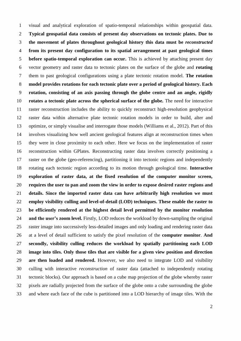
visual and analytical exploration of spatio-temporal relationships within geospatial data. 1

Typical geospatial data consists of present day observations on tectonic plates. Due to 2

the movement of plates throughout geological history this data must be reconstructed 3

from its present day configuration to its spatial arrangement at past geological times 4

before spatio-temporal exploration can occur. This is achieved by attaching present day 5

vector geometry and raster data to tectonic plates on the surface of the globe and rotating 6

them to past geological configurations using a plate tectonic rotation model. The rotation 7

model provides rotations for each tectonic plate over a period of geological history. Each 8

rotation, consisting of an axis passing through the globe centre and an angle, rigidly 9

rotates a tectonic plate across the spherical surface of the globe. The need for interactive 10

raster reconstruction includes the ability to quickly reconstruct high-resolution geophysical 11

raster data within alternative plate tectonic rotation models in order to build, alter and 12

optimize, or simply visualise and interrogate those models (Williams et al., 2012). Part of this 13

involves visualizing how well ancient geological features align at reconstruction times when 14

they were in close proximity to each other. Here we focus on the implementation of raster 15

reconstruction within GPlates. Reconstructing raster data involves correctly positioning a 16

raster on the globe (geo-referencing), partitioning it into tectonic regions and independently 17

rotating each tectonic region according to its motion through geological time. Interactive 18

exploration of raster data, at the fixed resolution of the computer monitor screen, 19

requires the user to pan and zoom the view in order to expose desired raster regions and 20

details. Since the imported raster data can have arbitrarily high resolution we must 21

employ visibility culling and level-of-detail (LOD) techniques. These enable the raster to 22

be efficiently rendered at the highest detail level permitted by the monitor resolution 23

and the user’s zoom level. Firstly, LOD reduces the workload by down-sampling the original 24

raster image into successively less-detailed images and only loading and rendering raster data 25

at a level of detail sufficient to satisfy the pixel resolution of the computer monitor. And 26

secondly, visibility culling reduces the workload by spatially partitioning each LOD 27

image into tiles. Only those tiles that are visible for a given view position and direction 28

are then loaded and rendered. However, we also need to integrate LOD and visibility 29

culling with interactive reconstruction of raster data (attached to independently rotating 30

tectonic blocks). Our approach is based on a cube map projection of the globe whereby raster 31

pixels are radially projected from the surface of the globe onto a cube surrounding the globe 32

and where each face of the cube is partitioned into a LOD hierarchy of image tiles. With the 33

3

cube map approach the rendering of a reconstructed raster follows a decoupled two-stage 1

process. Both stages take advantage of the ability of graphics hardware to rapidly project and 2

render a three-dimensional scene into a frame buffer (or target texture). The first stage renders 3

the geo-referenced raster into one or more tile textures of the cube map. The second stage 4

involves un-projecting those cube map tile textures back onto the globe during the rendering 5

of rotated tectonic surface regions. This separation of rendering stages simplifies the 6

implementation of raster reconstruction on the 3D globe while also enabling enhancements 7

such as raster reconstruction in different 2D map projections and combining multiple rasters. 8

Virtually all graphics hardware manufactured in the last decade has dedicated hardware to 9

accelerate transformations using 4x4 matrices. The cube map approach takes advantage of this 10

since each individual cube map tile has its own cube map projection transform represented as 11

an off-axis perspective 4x4 matrix. This enables GPlates to reconstruct and display arbitrary 12

resolution raster data at interactive frame rates on a wide variety of computer systems. 13

14

2 Multi-resolution raster visualization 15

GPlates initially uses a multi-resolution raster rendering approach when data are loaded into 16

GPlates, i.e when the user has chosen not or not yet to reconstruct a raster. Additionally, when 17

the user does choose to reconstruct a raster, this approach is used as the first stage of the raster 18

reconstruction process (to render that raster into a cube map). 19

2.1 Source raster data 20

In order to display raster data in GPlates a raster file needs to be imported. The import 21

procedure generates a GPML file with a single raster feature containing a link to the original 22

raster image file and raster meta-information including geo-referencing, coordinate reference 23

system and general raster metadata (Qin et al., 2012). GPlates uses the Geospatial Data 24

Abstraction Library (GDAL), an open-source library for raster geospatial data formats 25

(Warmerdam, 2008), for importing raster data. Source raster data from a variety of colour 26

image formats containing Red Green Blue Alpha (RGBA) colour data (including JPEG and 27

PNG) can be imported into GPlates. Also a variety of numerical image formats containing 28

floating-point or integer data (including NetCDF and GeoTIFF) can be imported. Both types 29

of raster data can be visualized in RGBA format - for numerical raster data (which has no 30

4

colour information) the user also selects a colour palette to translate from numerical pixels to 1

RGBA pixels. 2

2.2 Rationale for multi-resolution raster data 3

GPlates takes advantage of the power of graphics hardware to achieve raster rendering at 4

interactive frame rates. However the raster data still needs to be retrieved from storage before 5

it can be rendered. Since this is usually a Hard Disk Drive (HDD) with mechanical disk 6

platters this is by far the slowest component in raster visualization. More recently Solid 7

State Drives (SSD) are becoming less expensive and their random access reads have 8

much lower latencies than in HDDs. However HDD and SDD bandwidths are still 9

comparable so loading the entire raster into system memory is not desirable since this 10

can consume an excessive amount of time and computer memory. Especially since GPlates 11

supports arbitrarily high raster image resolutions (such as one minute global grids and higher) 12

which can exceed the maximum of 3-4 GB of virtual memory addressable by a 32-bit 13

application (even if the system has much more physical memory). 14

Therefore it is important to only interactively load raster data that is both (i) at a resolution 15

closely matching that of the desktop monitor (or visual display screen), and (ii) that is visible 16

in the view window. This level-of-detail and visibility culling is achieved with a multi-17

resolution tiled raster image pyramid that significantly reduces the amount of raster data 18

streamed from disk and reduces the rendering workload for the graphics hardware. 19

2.3 Multi-resolution tiled raster image pyramid 20

The raster image pyramid is generated by successively filtering the full resolution raster 21

image into progressively smaller versions of itself with each pyramid level halving the 22

dimension of the previous level (for example 4000x2000, 2000x1000, 1000x500, …). Since 23

this filtering is generally expensive it is only done once and written to a cache file (when the 24

raster is first rendered) such that subsequent sessions use the cache file directly. It should be 25

noted that this cache file resides on disk and not in memory. 26

During raster rendering GPlates selects the lowest resolution image that achieves a sharp and 27

crisp visual appearance of the raster (of course when even the highest detail resolution of the 28

raster is insufficient the raster cannot appear sharp and crisp). For example if the entire raster 29

is visible in the view window (when the view is fully zoomed out) and the full resolution 30

5

raster (level 0) has dimensions 21,600 x 10,800 (a one minute global grid) and the display 1

screen has dimensions 1,650 x 1,050 then the down-sampled image at level 3 in the pyramid 2

(of dimensions 2,700 x 1,350) is sufficient to display the raster without visual loss of detail. 3

In the above example the view was fully zoomed out to display the entire globe (or raster) 4

requiring only a low-resolution raster pyramid level to be loaded and rendered. The opposite 5

scenario occurs when the view is fully zoomed in to observe, in detail, a specific localised 6

geographic region. Here a much higher raster level of detail is required but a correspondingly 7

smaller area of the globe (or raster) is visible in the view window - essentially the majority of 8

the raster is not actually visible. To enable visibility culling, each image in the pyramid is 9

partitioned into small fixed-size tiles and only the visible tiles are loaded and rendered. Note 10

that all tiles contain the same number of pixels regardless of their pyramid level and hence 11

place the same load on the system (graphics hardware and streaming). 12

Interactive visualization is then possible because the total number of tiles loaded and rendered 13

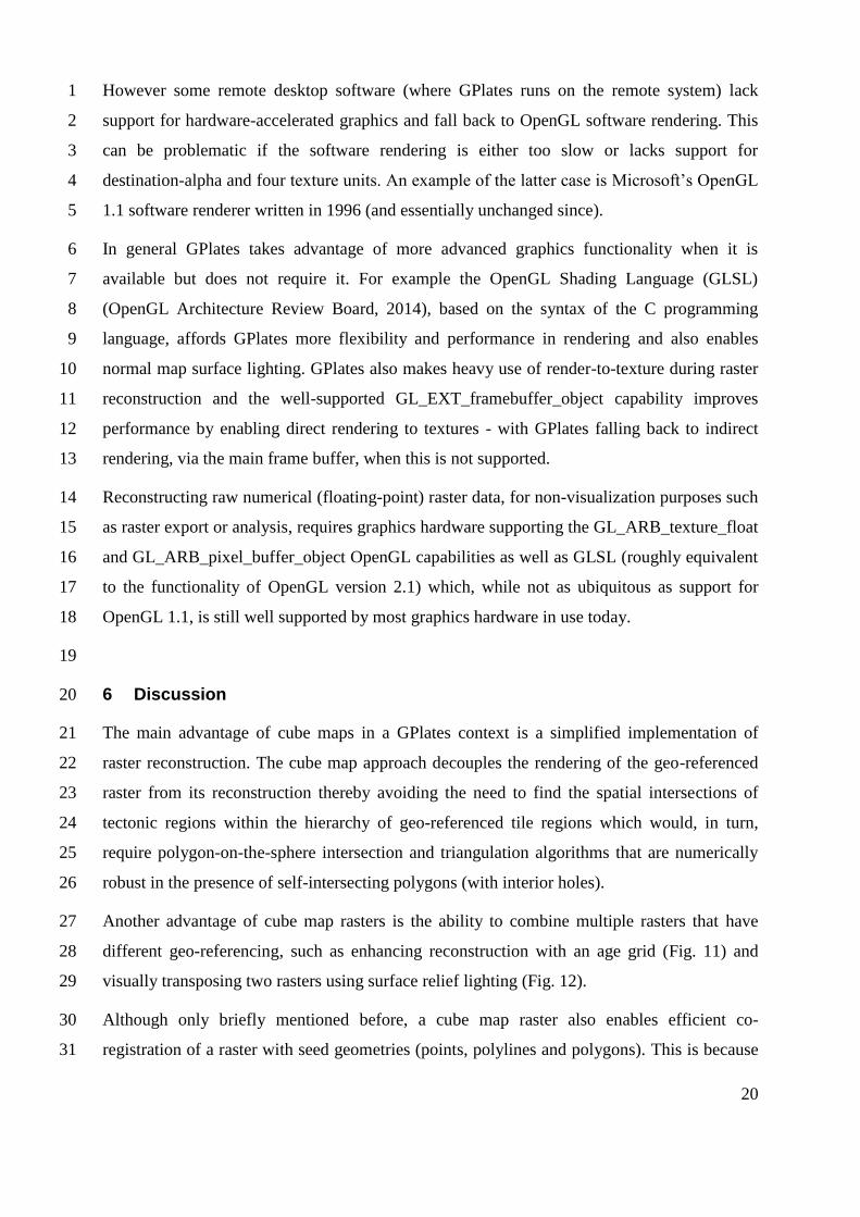
at any time is essentially bounded regardless of the zoom level. Figure 1 shows the visible 14

tiles of a raster as solid colours to highlight the tile partitioning. The left side of the figure 15

(showing the more zoomed-out view) exposes a larger area of the raster but conversely it can 16

use tiles from a lower resolution image in the pyramid. The right side of the figure (showing 17

the more zoomed-in view) exposes a smaller area of the raster but conversely it needs tiles 18

from a higher resolution image in the pyramid. As can be seen in Fig. 1C this results in both 19

zoom levels requiring roughly the same number of tiles and hence placing roughly the same 20

load on the graphics hardware and streaming sub-systems. The yellow wireframe in the figure 21

is the view frustum used by the “3D Orthographic” view in GPlates. A frustum, as typically 22

used in computer graphics for a perspective projection, is the solid portion of a truncated 23

pyramid whose top has been cut off by a plane parallel to its base (Neider et al., 1997) and 24

where the pyramid apex represents the eye, or camera, location (the single point receiving the 25

converging light rays). However the frustum in an orthographic view is a rectangular prism 26

(the light rays are parallel, instead of converging, and hence the eye/camera location is 27

essentially at infinity). The yellow orthographic view frustum in Fig. 1 does not include the 28

rear hemisphere of the globe because raster data on the rear hemisphere are not normally 29

visible through the globe (note that the globe is normally opaque grey in GPlates but is 30

rendered semi-transparent in the figure in order to highlight the yellow wireframe frustum 31

within the interior of the globe). 32

6

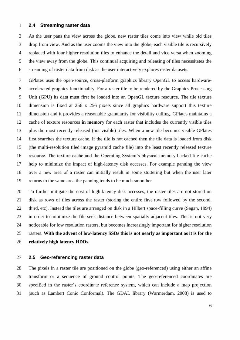
2.4 Streaming raster data 1

As the user pans the view across the globe, new raster tiles come into view while old tiles 2

drop from view. And as the user zooms the view into the globe, each visible tile is recursively 3

replaced with four higher resolution tiles to enhance the detail and vice versa when zooming 4

the view away from the globe. This continual acquiring and releasing of tiles necessitates the 5

streaming of raster data from disk as the user interactively explores raster datasets. 6

GPlates uses the open-source, cross-platform graphics library OpenGL to access hardware-7

accelerated graphics functionality. For a raster tile to be rendered by the Graphics Processing 8

Unit (GPU) its data must first be loaded into an OpenGL texture resource. The tile texture 9

dimension is fixed at 256 x 256 pixels since all graphics hardware support this texture 10

dimension and it provides a reasonable granularity for visibility culling. GPlates maintains a 11

cache of texture resources in memory for each raster that includes the currently visible tiles 12

plus the most recently released (not visible) tiles. When a new tile becomes visible GPlates 13

first searches the texture cache. If the tile is not cached then the tile data is loaded from disk 14

(the multi-resolution tiled image pyramid cache file) into the least recently released texture 15

resource. The texture cache and the Operating System’s physical-memory-backed file cache 16

help to minimize the impact of high-latency disk accesses. For example panning the view 17

over a new area of a raster can initially result in some stuttering but when the user later 18

returns to the same area the panning tends to be much smoother. 19

To further mitigate the cost of high-latency disk accesses, the raster tiles are not stored on 20

disk as rows of tiles across the raster (storing the entire first row followed by the second, 21

third, etc). Instead the tiles are arranged on disk in a Hilbert space-filling curve (Sagan, 1994) 22

in order to minimize the file seek distance between spatially adjacent tiles. This is not very 23

noticeable for low resolution rasters, but becomes increasingly important for higher resolution 24

rasters. With the advent of low-latency SSDs this is not nearly as important as it is for the 25

relatively high latency HDDs. 26

2.5 Geo-referencing raster data 27

The pixels in a raster tile are positioned on the globe (geo-referenced) using either an affine 28

transform or a sequence of ground control points. The geo-referenced coordinates are 29

specified in the raster’s coordinate reference system, which can include a map projection 30

(such as Lambert Conic Conformal). The GDAL library (Warmerdam, 2008) is used to 31

7

convert geo-referenced coordinates to the default coordinate reference system WGS 84 1

(Kumar, 1988) in GPlates. 2

GPlates uses OpenGL to render a raster tile by first creating a regular surface mesh containing 3

geo-referenced vertices and attaching the tile’s texture. Each vertex in the mesh contains a 3D 4

position on the globe and a 2D texture coordinate (location in the tile texture). Since the geo-5

referencing cannot be calculated at each raster pixel it is only accurate at mesh vertices. To 6

help minimize this visual deviation between vertices, adjacent vertices are separated by no 7

more than 16 pixels. Therefore one raster tile (256 x 256 pixels) is represented by a mesh of 8

17 x 17 vertices (including tile boundary vertices). Figure 2 illustrates how the mesh spacing 9

adapts to the level in the raster image pyramid such that the number of raster pixels between 10

adjacent mesh vertices is roughly the same (in Fig. 2A and Fig. 2B). 11

2.6 Rendering raster data 12

Rendering a raster involves first determining the resolution level in the multi-resolution image 13

pyramid and then finding the visible geo-referenced tiles in that level. To determine tile 14

visibility, each tile is bounded by an Oriented Bounding Box (OBB) that is tested for 15

intersection with the view frustum. An OBB is a rectangular 3D bounding box at an arbitrary 16

orientation. To improve culling efficiency all tiles in each resolution level are arranged in an 17

OBB binary tree so that, during rendering, hierarchical visibility culling can be employed to 18

cull an entire group of tiles with a single OBB-Frustum test. The visible raster tiles are then 19

rendered into the view window or, if the raster is reconstructed, into the cube map. 20

2.7 Time-dependent rasters 21

A raster consists of a single raster image typically representing geospatial data observations 22

on the Earth’s present-day surface. GPlates can also create a time-dependent raster by 23

importing a time sequence of raster image files and assigning geological ages to each image. 24

GPlates renders a time-dependent raster by selecting the image, in its time sequence, whose 25

age most closely matches the current geological time. Note that it is also possible to 26

reconstruct a time-dependent raster. In this case both the image and spatial location of the 27

time-dependent raster vary with geological time. Raster reconstruction is covered in the next 28

section. 29

30

8

3 Multi-resolution raster reconstruction 1

The rendering framework described so far can render an unreconstructed raster either 2

directly to the computer screen when the user has chosen not to reconstruct a raster or 3

as the first stage of the raster reconstruction process when the user does choose to 4

reconstruct a raster. 5

This section describes our approach to visualisation of a reconstructed present-day (or time-6

dependent) raster by building a multi-resolution cube map framework on top of the raster 7

rendering framework described so far. 8

Our raster reconstruction process involves a multi-resolution cube map, a set of tectonic 9

polygons and a rotation model. By imprinting the raster data into the overlapping 10

tectonic polygons and then independently rotating the polygons across the globe, using 11

the rotation model, we are essentially reconstructing present day raster data to its past 12

geological configuration. First we introduce the concept of a cube map as an efficient 13

way to capture raster data in a representation that is decoupled from the raster’s geo-14

referencing and inbuilt raster projection. We then extend the cube map with multi-15

resolution tiles to support level-of-detail and visibility culling necessary for efficient 16

rendering. We show that any tile, in the cube map, can be generated by rendering the 17

geo-referenced raster using the method described in Sect. 2. With the generation of a 18

multi-resolution cube map covered, we finally describe in detail how raster data are 19

imprinted onto tectonic polygons and rotated with them across the globe. The multi-20

resolution cube map facilitates this by enabling the raster imprinting, of pre-rendered 21

cube map tiles onto tectonic polygons, to be accelerated by common graphics hardware. 22

3.1 Cube map properties 23

The cube map was first proposed by Ned Greene (Greene, 1986) as an alternative method of 24

capturing the full projection of the world or environment from a particular world location. 25

This is useful for applications such as reflection mapping because the cube map can be 26

efficiently generated and indexed using common graphics hardware (compared to spherical 27

and paraboloid mappings). An environment cube map is created by placing the cube centre at 28

a particular world location and then projecting the environment onto the six faces of the cube. 29

This is achieved by separately rendering the six views into six square textures each using a 30

90º field-of-view perspective frustum. The environment cube map then consists of these six 31

9

textures arranged as a single hardware cube map texture (since the GeForce256 GPU was 1

introduced in 1999) whereby a 3D direction vector can be used to lookup the cube map 2

texture. For example, in the reflection mapping scenario the 3D lookup vector is a surface 3

reflection vector calculated at each point on the reflecting object’s surface such that when the 4

entire surface is rendered it will appear to reflect the environment. 5

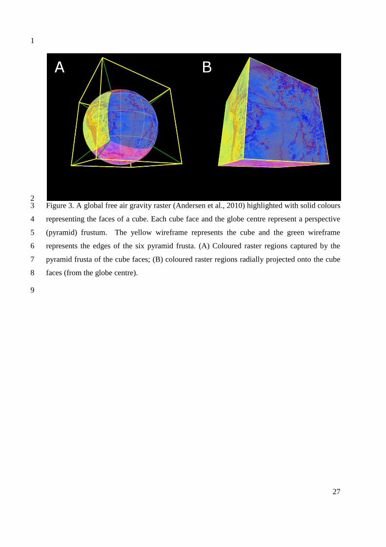
For GPlates the cube centre is always positioned at the centre of the globe and the 6

environment captured by the cube map is the raster data as it appears on the surface of the 7

globe. Essentially we’re looking from the centre of the globe at the inside of the globe as if 8

the interior of the globe was empty and the raster was painted on the inside surface of the 9

globe. The view direction of each of the six view frustums is aligned with a coordinate system 10

axis (+x, -x, +y, -y, +z, -z). Figure 3 shows a global raster captured in an environment cube 11

map. 12

Once the raster cube map is captured it can then be accessed using a 3D vector to lookup a 13

raster pixel. The 3D lookup vector is simply the direction from the centre of the globe to a 14

point on the surface of the globe. For a unit sphere centred at the coordinate system origin this 15

is the same as the 3D position on the surface of the globe. The raster pixel retrieved from the 16

cube map is the value of the geo-referenced raster at the specified surface position on the 17

globe. 18

A cube map has a higher sampling density near the face corners compared with the face 19

centres resulting in a non-uniform sampling of the cube map pixels across the surface of the 20

globe. However the non-uniformity is much less than the common rectangular 21

(latitude/longitude) projection and avoids the projection singularity at the North and South 22

Poles. 23

3.2 A multi-resolution cube map 24

Essentially a cube map raster and a geo-referenced raster are different representations of the 25

same raster data. So, as with the geo-referenced raster, the cube map raster is extended to 26

include multi-resolution capabilities. That is, to enable matching the cube map raster 27

resolution to the display (or render target) resolution and to enable visibility culling by 28

partitioning each face of the cube into tiles. 29

A multi-resolution cube map hierarchically partitions each face of a cube into tiles using a 30

quadtree data structure (Finkel and Bentley, 1974) whereby the two-dimensional surface of 31

10

each cube face is divided into four quadrants and each quadrant further divided into four sub-1

quadrants and so on. Each node in the quadtree represents a fixed-dimension tile. Each level, 2

or depth, in the quadtree represents a different resolution of the cube map raster since each 3

level contains, relative to its parent level, four times the number of tiles (and hence four times 4

the pixels). For example if the tile dimension is 256 then quadtree level 0 is one tile (or 256 x 5

256 pixels), level 1 is 2 x 2 tiles (or 512 x 512 pixels), level 2 is 4 x 4 tiles (or 1024 x 1024 6

pixels), etc. Figure 4 shows the association between the quadtree data structure, the hierarchy 7

of tile images and the tile frustums within a single cube face. Also note that there are six 8

quadtrees in total since each cube face has its own quad tree. 9

3.3 Generating a cube map raster 10

A cube map raster is generated by rendering a geo-referenced raster into it. This uses the same 11

rendering procedure that was used to render a geo-referenced raster into the view window, as 12

described in Sect. 2, with the exception that the view frustum and target frame buffer differ 13

for the cube map. Each tile in a multi-resolution cube map has its own view frustum and 14

target texture resource. A cube map tile texture is generated by rendering only those geo-15

referenced tiles that are visible in its view frustum. During rendering, the geo-referenced tile 16

vertices are transformed by the 4x4 off-axis perspective (pyramid) projection transformation 17

(Neider et al., 1997) defined by the frustum of that cube map tile. Figure 5 shows the geo-18

referenced tiles, as solid colours, visible in the view frustum of a single cube map tile. 19

A cube map raster contains all such cube map tiles whose frusta intersect the geo-referenced 20

raster (for a global raster this includes all cube map tiles). Figure 6 shows these cube map tiles 21

for a regional geo-referenced raster at three different resolution levels. Only those cube map 22

tiles that actually cover the raster’s region are required. Note that the solid colours in Fig. 6 23

highlight the cube map tiles as opposed to Fig. 5 which highlights the geo-referenced tiles (for 24

a single cube map tile). 25

For graphics hardware supporting non-power-of-two texture dimensions the tile dimension of 26

the cube map is optimally adapted for each geo-referenced raster in order to minimize texture 27

memory usage. 28

11

3.4 Rendering reconstructed raster data 1

Raster data are reconstructed by combining a raster cube map, a tectonic polygon dataset and 2

a rotation model. A tectonic polygon represents the boundary of a tectonic plate - a region of 3

the Earth’s crust that is typically rigid throughout geological time. The rotation model 4

determines the motion of each tectonic plate across the globe over geological time. Each 5

tectonic polygon is linked to the rotation model using a tectonic plate ID which provides 6

access to a time sequence of finite Euler rotations (Boyden et al., 2011;Greiner, 1999) that 7

rotate the tectonic plate from its present day position to its position at a time in the geological 8

past relative to another tectonic plate (with a different plate ID). These plate-relative rotations 9

are then accumulated by traversing the plate circuit from the tectonic plate back to the global 10

reference frame to obtain the absolute rotation of the tectonic plate (Cox and Hart, 1986). Any 11

geospatial data, including rasters, attached to a tectonic plate will inherit that plate’s motion 12

over geological time. Vector geometry such as points, polylines and polygons can be 13

reconstructed once they are partitioned into tectonic plates (and assigned associated plate 14

IDs). Raster data is conceptually reconstructed in a similar manner whereby raster pixels are 15

attached to (or partitioned into) tectonic plates and then rotated using the motion of the 16

attached plates. In GPlates the user attaches raster data to tectonic plates by connecting a 17

polygon layer to a raster layer. Although the tectonic plates can rotate across the globe, their 18

polygon shapes are static (not change over time). While GPlates does support dynamic plate 19

polygons (Gurnis et al., 2012) to handle the changing shape of oceanic plates over geological 20

time, they are not currently used to reconstruct rasters. A future extension of GPlates 21

functionality will be designed to use dynamic plate polygons, along with deforming plates, to 22

reconstruct and deform rasters. 23

A raster is efficiently reconstructed by mapping the tile textures of the raster cube map onto 24

the tectonic plate polygons and compositing the rotated polygon-tile intersections into the 25

scene. The level-of-detail selected for rendering is the lowest resolution of the raster cube map 26

that maintains a crisp visual appearance of the reconstructed raster. Figure 7 shows the 27

pseudocode for rendering a reconstructed raster. 28

The function render_reconstructed_raster iterates over the six faces of the raster 29

cube map and, for each tectonic polygon, renders those cube map tiles (at the appropriate 30

level-of-detail) that overlap the polygon. Each face of the cube map contains a quadtree 31

hierarchy of tiles that, beginning with the root tile of a face, is recursively visited using the 32

12

function render_raster_tile. Each level of recursion visits one level deeper in the 1

quadtree and expands the number of tiles visited by up to four. If a visited tile is at the 2

appropriate level of the quadtree for rendering then the tile is mapped onto the polygon and 3

then rotated and composited into the scene. Otherwise the four child tiles at the next deeper 4

level are visited recursively. Tiles that do not overlap the polygon are culled, and rotated tiles 5

that are not visible are also culled. 6

Figure 8 shows the accumulated rendering of a single rotated polygon mesh. The rendering 7

level-of-detail is quadtree level 1. At this detail level there are three tiles overlapping the 8

polygon. Those same three tiles are also shown in their present day locations in Fig. 6B. 9

This process is repeated for all tectonic polygons until the reconstructed raster is fully 10

composed into the scene. Figure 9 shows a raster reconstructed with two tectonic plates. 11

The following sections cover the most important details in this process. 12

3.4.1 Generating tectonic polygon triangulation meshes 13

Each tectonic polygon is rendered as a spherical mesh that is triangulated within the interior 14

surface region of the polygon. The Computational Geometry Algorithms Library (CGAL) 15

(Fabri and Pion, 2009) is used to generate a surface polygon mesh of sufficient tessellation to 16

give a spherical appearance when rendering into the “3D Orthographic” view in GPlates. This 17

is a time-consuming process and as such it only occurs when a raster layer is first connected 18

to a polygon layer in GPlates. Figure 8 (B,D,F) shows the wireframe of continental Australia. 19

Since the cube map decouples geo-referenced raster rendering (Sect. 2) from tectonic polygon 20

rendering, the same tectonic polygon mesh dataset can be shared by all raster layers attached 21

to it. 22

3.4.2 Mapping a raster cube map onto polygon meshes 23

In the pseudocode in Fig. 7 each atomic rendering operation submitted to OpenGL consists of 24

a rotated polygon mesh rendered with a cube map tile texture. In most applications a texture is 25

usually mapped onto a mesh by assigning a 2D texture coordinate to each mesh vertex. An 26

advantage of the cube map approach is the tectonic polygon meshes can be rendered without 27

requiring explicit texture coordinates. Instead the surface positions in the mesh vertices are 28

transformed to texture coordinates directly by the graphics hardware during polygon mesh 29

rendering. Automatic texture coordinate generation dates back to base OpenGL 1.1 and 30

13

supports matrix transformation of vertex positions for use as texture coordinates. GPlates uses 1

this functionality to project the 3D position of each polygon mesh vertex into the 2D texture 2

space of a cube map tile. This 4x4 texture matrix transformation is identical to the matrix used 3

to render the geo-referenced raster into the cube map tile texture. This has the same effect as 4

un-projecting the pre-rendered cube map tile texture back onto the globe during rendering of 5

the surface polygon mesh. Note that the graphics hardware uses perspective-correct texture 6

coordinate interpolation when rasterizing pixels (of the polygon mesh) and hence there is no 7

texture projection deviation or mismatch between generating a cube map tile texture (Sect. 8

3.3) and un-projecting it back onto the globe. 9

In addition to transforming the 3D positions of mesh vertices to generate 2D texture 10

coordinates, the 3D positions are transformed to generate the final rotated polygon mesh 11

positions on the surface of the globe using the Euler rotation of the tectonic polygon. The 12

combined effect of these two transformations is to project a raster onto a polygon mesh and 13

then rotate it across the globe. Both 4x4 transformations are accelerated by the graphics 14

hardware. 15

3.4.3 Clipping polygon meshes to cube map tiles 16

Graphics hardware can apply a limited number of textures when rendering a mesh (with older 17

hardware supporting a maximum of four textures). Each cube map tile is rendered using up to 18

four textures in some cases, including the source tile texture itself, the clip texture (see below) 19

and an optional age grid mask and age grid coverage texture (age grids are described in Sect. 20

4.3). So even though a single polygon mesh can overlap multiple cube map tiles, it must be 21

rendered separately for each tile. In this case only the intersection of a polygon mesh with 22

each cube map tile can be rendered. This is achieved by rendering the entire polygon mesh for 23

each cube map tile but only rasterizing pixels that map to a tile’s interior. Pixels that map to a 24

tile’s exterior are rejected by modulating the tile’s texture with a clip texture and using the 25

Alpha Test functionality of OpenGL 1.1 to discard transparent pixels (alpha equal to zero). 26

The clip texture is a small 4x4 pixel texture containing opaque inner pixels and transparent 27

outer pixels. The boundary around the inner 2x2 pixels maps to the tile boundary such that 28

polygon mesh regions outside the tile become transparent.Figure 8 (B,D,F) illustrates the 29

clipping of a single rotated polygon mesh by the three tiles that overlap it. 30

14

3.4.4 Intersections between cube map tiles and tectonic polygons 1

The pseudocode in Fig. 7 includes a test for the intersection of a present-day (un-rotated) 2

tectonic polygon with an un-rotated cube map tile. These intersections are independent of the 3

geological time of reconstruction since they do not involve rotations and hence their boolean 4

results can be pre-computed for all tile-polygon pairs. And since the tile partitioning spatial 5

configuration is the same for all raster cube maps, regardless of their individual geo-6

referencing, the intersection results can be shared by all rasters that are attached to the same 7

tectonic polygon dataset. 8

3.4.5 Visibility culling of cube map tiles 9

The pseudocode in Fig. 7 includes a test to determine if a rotated tile is visible in the scene’s 10

view frustum when rendering a tectonic polygon. Each cube map tile is bounded by an 11

Oriented Bounding Box (OBB) in much the same way as geo-referenced tiles are bounded 12

(Sect. 2.6). Visibility culling involves rotating the OBB of each cube map tile that overlaps a 13

tectonic polygon (using the Euler rotation of the tectonic polygon). A rotated tile is then only 14

rendered if its rotated OBB intersects the scene’s view frustum. Figure 8 (A,C,E) shows the 15

rotated tile OBBs in red wireframe and the scene’s view frustum in yellow wireframe. As 16

with geo-referenced tiles the visibility culling is hierarchical since a single OBB-Frustum test 17

can cull an entire sub-tree of quadtree tiles. Also it turns out that, instead of rotating each tile 18

OBB, it is actually more efficient to reverse-rotate the scene view frustum once (per tectonic 19

polygon) and hierarchically test against the un-rotated OBBs. A single polygon typically has 20

multiple overlapping tiles. Conversely a single tile can be covered by multiple (adjacent) 21

polygons. 22

3.4.6 Removing texture seams between cube map tiles 23

Cube map tile textures are rendered using hardware bilinear filtering to reduce the texture 24

sampling artifacts of nearest-neighbour filtering. However this introduces visible raster seams 25

or discontinuities across tile boundaries because the filtered texture samples of two adjacent 26

tiles do not match along the shared tile boundary. To remove these seams each cube map tile 27

frustum is expanded by half a pixel such that adjacent tile frusta overlap slightly. Note that 28

this does not introduce a half-pixel error because the geo-referenced raster is also rendered 29

into the adjusted frusta when generating the cube map tiles. 30

15

Since GPlates adapts the raster cube map resolution to the display (or render target), hardware 1

texture mipmaps (Williams, 1983) are not required to reduce frequency aliasing artifacts. This 2

also avoids the problem of the half pixel frusta overlap solution not always working with 3

hardware texture mipmaps (due to pixel size varying across mipmap levels). However 4

hardware anisotropic texture filtering is used to reduce aliasing in highly anisotropic regions 5

of the globe where the surface normal is almost perpendicular to the view direction (such as 6

near the horizon). 7

8

4 Raster reconstruction enhancements 9

The rendering framework described so far can render a reconstructed raster directly to 10

the computer screen in the standard 3D globe view. This section describes various 11

enhancements to raster reconstruction that build on the approach described in Sect. 3. 12

Visualising reconstructed rasters in the 2D map projection views discusses how 13

interactivity is maintained in the 2D map views. Instead of rendering the reconstructed 14

raster directly to the computer screen (as done in the 3D globe view) it is first rendered 15

into an intermediate cube map (called the reconstructed cube map) and then rendered 16

directly to the computer screen via a map projection. 17

Improved raster reconstruction using age grids makes use of a second raster containing 18

pixel values representing the age of oceanic crust. Replacing the usual per-tectonic-19

polygon age test with a per-pixel age test restores the missing sections of reconstructed 20

raster data near oceanic ridges. 21

Revealing raster detail with surface normal maps modulates the colour of a raster with 22

the surface lighting generated from a second raster. This enables patterns in the second 23

raster to be visually transposed onto the first raster. 24

And finally, analysing reconstructed numerical raster data adds support for 25

reconstructing floating-point raster data (in contrast to colour raster data). This enables 26

numerical raster data to be analysed in the data-mining front-end of GPlates and also 27

enables export to numerical raster file formats. 28

16

4.1 Visualising reconstructed rasters in 2D map projection views 1

The default view in GPlates is the 3D Orthographic Globe view that uses an orthographic 2

view projection commonly used in Computer-aided Design (CAD) software where the lines 3

of projection are parallel. GPlates also supports a variety of 2D map projection views 4

including the Rectangular, Mercator, Mollweide and Robinson projections that un-wrap the 5

globe onto a 2D plane. 6

Rendering reconstructed raster data to a 2D map view requires an extra rendering phase above 7

that required for the 3D globe view. Instead of rendering directly to the computer screen (as 8

done for the 3D globe view) the reconstructed raster is rendered into a reconstructed cube 9

map which is, in turn, rendered to the 2D map view. This also serves to demonstrate that a 10

cube map can capture any surface representation on the globe. The cube map in Sect. 3.3 11

captures the un-reconstructed, geo-referenced raster. Here the reconstructed cube map 12

captures the final reconstructed raster (the output of Sect. 3.4). The 3D globe view does not 13

need a reconstructed cube map because the 3D orthographic view projection and each tectonic 14

polygon Euler rotation can be combined into a single 4x4 matrix that can be accelerated by 15

graphics hardware dating back to OpenGL 1.1. For the 2D map views the surface positions on 16

the globe are converted into 2D map coordinates using the Proj4 library (Evenden and 17

Warmerdam, 1990) and this library cannot be offloaded to the graphics hardware. Even if that 18

were possible the graphics hardware would still need to clip the rotated tectonic polygons 19

across the 2D map boundary and this is not something that most graphics hardware can do. 20

While this could all be done on the Central Processing Unit (CPU) it would be significantly 21

slower. Instead the alternate solution of rendering to a reconstructed cube map keeps the 2D 22

map views interactive by decoupling raster reconstruction from map projection. This removes 23

the need to perform expensive per-vertex map projections for each rendered frame and 24

removes the need to clip rotated tectonic polygon meshes to the 2D map boundary (the 25

reconstructed cube map is aligned with the central meridian of the map projection). The 26

contents of the reconstructed cube map are rendered to the 2D map view using a static 27

latitude/longitude mesh with each vertex containing a 2D map view position and its 28

associated 3D position on the globe. To access the reconstructed raster data the graphics 29

hardware projects the 3D position, in each vertex, into a reconstructed cube map tile texture. 30

The mesh tessellation is dense enough to provide a visually accurate sampling of the map 31

projection. And tile LOD determination and visibility culling for a 2D map view is done using 32

17

the hierarchical partitioning of the reconstructed cube map (in a similar manner to that 1

described in Sect. 3). 2

Figure 10 shows a raster reconstructed with two tectonic plates in a 2D map projection view 3

(similar to Fig. 9 which instead uses the 3D orthographic view). Note that, unlike Fig. 9C, the 4

cube map tiles in Fig. 10C do not retain their shape after rotation. This is due to the 2D map 5

projection and is particularly noticeable with Antarctica. 6

4.2 Combining multiple rasters 7

So far we have dealt with a single reconstructed source raster. In sections 4.3 and 4.4 new 8

rasters are introduced that are combined with the source raster in different ways. However two 9

rasters cannot easily be combined if they have different geo-referencing or different raster 10

inbuilt map projections. This is because the geo-referenced tiles of two different rasters will 11

not, in general, be aligned across the two rasters or projected in the same way and hence 12

cannot be paired or associated. But since all rasters have the same cube map spatial 13

partitioning, regardless of their individual geo-referencing, they can be combined after their 14

cube maps have been generated. And this procedure is used for age grids and surface normal 15

maps in the following sections. 16

4.3 Enhancing raster reconstruction with a crustal age grid 17

Each tectonic polygon has a time of appearance and disappearance corresponding to the 18

geological time period over which the crust, contained within the interior of the polygon, 19

existed on the Earth’s surface. The pseudocode in Fig. 7 renders only the subset of tectonic 20

polygons that exist at a particular reconstruction time. In order to simulate the gradual 21

generation of oceanic crust at mid-ocean ridges, many long, thin oceanic polygons with 22

varying times of appearance have been digitised along these ridges. These oceanic polygons 23

progressively appear as GPlates animates the reconstruction time forward in time. However 24

the granularity of this transition is still quite coarse with regions (the size of polygons) 25

continually popping into view. A finer per-pixel granularity is achieved by using an age grid 26

raster. 27

The age grid is a separate raster that contains the time of appearance in each pixel (Müller et 28

al., 2008). It follows the same principle as polygons but reduced in spatial extent to pixel size 29

regions of crust. The tectonic polygons are still used during raster reconstruction, but now the 30

18

per-polygon age comparison is replaced with a per-pixel age comparison effectively removing 1

the polygon popping. This per-pixel comparison is efficiently performed using the graphics 2

hardware. For OpenGL 2.0 hardware this test is simply a floating-point comparison in an 3

OpenGL Shading Language (OpenGL Architecture Review Board, 2014) shader program. For 4

older hardware some rendering trickery is required to simulate this comparison using fixed-5

point hardware and four texture units. Figure 11 shows the reconstruction of a raster with and 6

without the assistance of an age grid. 7

4.4 Enhancing visual detail with surface normal maps 8

A raster can be visually transposed onto another raster by combining the colour of the first 9

raster with the surface lighting of the second. The second raster is treated like a height-field 10

from which surface relief shading is generated. The colour of the first raster is then modulated 11

with the surface lighting (intensity) of the second raster to get the final output colour. Figure 12

12 shows two rasters that source lighting from themselves and from each other. Figure 12D 13

uses the age grid for surface relief (height-field) - the regions near the mid-ocean ridge 14

(between Africa and South America) appear to have a lower elevation than surrounding 15

regions due to the lower age grid values. 16

Surface lighting is recalculated and combined as the raster is reconstructed to geological 17

times. In other words surface relief shading is not pre-baked into the raster but calculated 18

interactively as diffuse lighting using the light direction and rotated surface normals. The 19

surface normal tiles are generated on-the-fly from raw numerical (height) raster data as an 20

extension of the streaming process (Sect. 2.4). This is done on the GPU to enhance 21

performance when floating-point textures and OpenGL Shading Language (OpenGL 22

Architecture Review Board, 2014) are supported. However these generated surface normals 23

are in the tangent space of the geo-referencing (aligned with the raster). When the geo-24

referenced surface normal raster is rendered into a cube map the surface normals are 25

converted to world space (aligned with the global Cartesian coordinate system). This enables 26

a surface lighting cube map to be combined with another raster cube map (since the raster-27

specific geo-referencing dependency has been removed). 28

19

4.5 Analyzing reconstructed numerical raster data 1

The GPU is typically a separate processor with its own high-speed memory for storing 2

working data (such as textures and rendered images). GPlates visualizes reconstructed 3

numerical (floating-point) raster data by first translating it to colour data before uploading to 4

the GPU as 8-bit-per-channel RGBA textures (supported by all graphics hardware). The 5

reconstructed RGBA raster data is then scanned straight from GPU memory to the display 6

screen. In this case the original (un-translated) floating-point raster data is not reconstructed. 7

This is fine for visualization however there are situations where GPlates needs to access the 8

reconstructed floating-point raster data itself. 9

Reconstructed raw numerical raster data is needed when GPlates exports to numerical image 10

file formats (such as NetCDF) for analysis by other software. It is also needed in the data-11

mining front-end of GPlates (Landgrebe and Muller, 2011) where raster data is co-registered 12

with seed geometries by applying operations (such as mean and standard deviation) to the 13

reconstructed numerical raster pixels within a region-of-interest of the seed geometries (the 14

details of which are beyond the scope of this article). 15

GPlates can reconstruct raw numerical raster data (as opposed to RGBA raster data) provided 16

the graphics hardware has support for floating-point textures. In this case numerical raster 17

data is first uploaded to the GPU as two-channel floating-point textures. One channel is used 18

for the floating-point raster data and the other is for the raster coverage or opacity. The 19

numerical raster data is then reconstructed on the GPU and rendered into floating-point target 20

textures. This reconstructed raster data is then asynchronously downloaded from the GPU 21

using pixel buffers (GL_ARB_pixel_buffer_object OpenGL extension) to avoid stalling the 22

Central Processing Unit (CPU) thereby allowing it to keep the GPU busy with subsequent 23

reconstruction tasks. 24

25

5 OpenGL in GPlates 26

GPlates can visualize reconstructed raster data on any graphics hardware manufactured in the 27

last decade. This is because raster reconstruction visualization requires only base OpenGL 1.1 28

functionality plus support for destination-alpha (for writing raster opacity to target textures) 29

and four texture units, which is well supported by all graphics hardware in that time period. 30

20

However some remote desktop software (where GPlates runs on the remote system) lack 1

support for hardware-accelerated graphics and fall back to OpenGL software rendering. This 2

can be problematic if the software rendering is either too slow or lacks support for 3

destination-alpha and four texture units. An example of the latter case is Microsoft’s OpenGL 4

1.1 software renderer written in 1996 (and essentially unchanged since). 5

In general GPlates takes advantage of more advanced graphics functionality when it is 6

available but does not require it. For example the OpenGL Shading Language (GLSL) 7

(OpenGL Architecture Review Board, 2014), based on the syntax of the C programming 8

language, affords GPlates more flexibility and performance in rendering and also enables 9

normal map surface lighting. GPlates also makes heavy use of render-to-texture during raster 10

reconstruction and the well-supported GL_EXT_framebuffer_object capability improves 11

performance by enabling direct rendering to textures - with GPlates falling back to indirect 12

rendering, via the main frame buffer, when this is not supported. 13

Reconstructing raw numerical (floating-point) raster data, for non-visualization purposes such 14

as raster export or analysis, requires graphics hardware supporting the GL_ARB_texture_float 15

and GL_ARB_pixel_buffer_object OpenGL capabilities as well as GLSL (roughly equivalent 16

to the functionality of OpenGL version 2.1) which, while not as ubiquitous as support for 17

OpenGL 1.1, is still well supported by most graphics hardware in use today. 18

19

6 Discussion 20

The main advantage of cube maps in a GPlates context is a simplified implementation of 21

raster reconstruction. The cube map approach decouples the rendering of the geo-referenced 22

raster from its reconstruction thereby avoiding the need to find the spatial intersections of 23

tectonic regions within the hierarchy of geo-referenced tile regions which would, in turn, 24

require polygon-on-the-sphere intersection and triangulation algorithms that are numerically 25

robust in the presence of self-intersecting polygons (with interior holes). 26

Another advantage of cube map rasters is the ability to combine multiple rasters that have 27

different geo-referencing, such as enhancing reconstruction with an age grid (Fig. 11) and 28

visually transposing two rasters using surface relief lighting (Fig. 12). 29

Although only briefly mentioned before, a cube map raster also enables efficient co-30

registration of a raster with seed geometries (points, polylines and polygons). This is because 31

21

the seed geometries are inserted into a spatial partition that follows a hierarchical cube map 1

structure analogous to that of the raster’s cube map. This enables spatial associations between 2

the raster and seed geometries to be quickly found. 3

A potential disadvantage of the cube map approach is that the intermediate cube map 4

generation phase results in an additional re-sampling stage that can reduce the quality of the 5

raster data due to the bilinear filtering. And for the 2D map views there is a further cube map 6

generation phase (Sect. 4.1) resulting in another re-sampling stage. 7

Another disadvantage is the non-uniform sampling of the cube map pixels that varies by a 8

factor of approximately two, or more accurately 3 / sqrt(2), from a cube face centre to one of 9

its corners. For some cube map tiles this can result in up to four (2x2) times as many pixels 10

rendered than is necessary for no loss of visual detail. This disadvantage does lessen for the 11

higher resolution LODs (since those tiles cover less area of each cube face). However the 12

flexibility gained by having a raster in cube map form is very advantageous. 13

7 Conclusions 14

This paper describes a method of reconstructing raster data that integrates a cube environment 15

map with multi-resolution tile partitioning. This enables on-demand tile streaming, level-of-16

detail rendering and hierarchical visibility culling to be applied to rasters reconstructed by 17

tectonic plate polygons. Furthermore the partitioned cube map tiles require only 4x4 matrix 18

transformations which are extremely well supported by graphics hardware. With this 19

implementation GPlates can reconstruct raster data on a wide variety of desktop and laptop 20

computers manufactured over the last decade enabling users to interactively visualise and 21

analyse arbitrarily high-resolution geophysical raster data for geological times in the past. 22

This capability forms the basis for interactively building and improving plate reconstructions 23

in an iterative fashion, for tectonically complex regions as well as for ancient supercontinent 24

assemblies, which can easily be analysed using GPlates by assigning geophysical grids and 25

geological data to individual tectonic elements and interactively testing their alignment in 26

alternative reconstructions (Williams et al., 2012). 27

28

29

Acknowledgements 30

22

RDM and JC were supported by ARC grant FL0992245, and JC and EL were also supported 1

by the AuScope National Collaborative Research Infrastructure (www.auscope.org.au/). 2

3

23

References 1

Amante, C., and Eakins, B. W.: ETOPO1 1 arc-minute global relief model: procedures, data 2

sources and analysis, US Department of Commerce, National Oceanic and Atmospheric 3

Administration, National Environmental Satellite, Data, and Information Service, National 4

Geophysical Data Center, Marine Geology and Geophysics Division, 2009. 5

Andersen, O. B., Knudsen, P., and Berry, P. A.: The DNSC08GRA global marine gravity 6

field from double retracked satellite altimetry, Journal of Geodesy, 84, 191-199, 2010. 7

Boyden, J. A., Müller, R. D., Gurnis, M., Torsvik, T. H., Clark, J. A., Turner, M., Ivey-Law, 8

H., Watson, R. J., and Cannon, J. S.: Next-generation plate-tectonic reconstructions using 9

GPlates, in: Geoinformatics: Cyberinfrastructure for the Solid Earth Sciences, edited by: 10

Keller, G. R., and Baru, C., Cambridge University Press, Cambridge, 95-114, 2011. 11

Cox, A., and Hart, B. R.: Plate Tectonics : How It Works, Blackwell Science Inc., 400 pp., 12

1986. 13

Fabri, A., and Pion, S.: CGAL: the Computational Geometry Algorithms Library, 14

Proceedings of the 17th ACM SIGSPATIAL International Conference on Advances in 15

Geographic Information Systems, Seattle, Washington, 2009, 538-539, 16

Finkel, R. A., and Bentley, J. L.: Quad trees a data structure for retrieval on composite keys, 17

Acta Informatica, 4, 1-9, 10.1007/BF00288933, 1974. 18

Goodwillie, A.: User guide to the GEBCO one minute grid, Centenary edition of the GEBCO 19

digital atlas, GEBCO, 2003. 20

Greene, N.: Environment Mapping and Other Applications of World Projections, Computer 21

Graphics and Applications, IEEE, 6, 21-29, 10.1109/MCG.1986.276658, 1986. 22

Greiner, B.: Euler rotations in plate-tectonic reconstructions, Computers & Geosciences, 25, 23

209-216, 1999. 24

Gurnis, M., Turner, M., Zahirovic, S., DiCaprio, L., Spasojevic, S., Muller, R. D., Boyden, J., 25

Seton, M., Manea, V. C., and Bower, D. J.: Plate tectonic reconstructions with continuously 26

closing plates, Computers & Geosciences, 38, 35-42, DOI 10.1016/j.cageo.2011.04.014, 27

2012. 28

Kumar, M.: World geodetic system 1984: A modern and accurate global reference frame, 29

Marine Geodesy, 12, 117-126, 10.1080/15210608809379580, 1988. 30

Landgrebe, T. C. W., and Muller, R. D.: A Spatio-Temporal Knowledge-Discovery Platform 31

for Earth-Science Data, Digital Image Computing Techniques and Applications (DICTA), 32

2011 International Conference on, 6-8 Dec. 2011, 394 – 399, 10.1109/DICTA.2011.73, 2011. 33

Müller, R. D., Sdrolias, M., Gaina, C., and Roest, W. R.: Age, spreading rates and spreading 34

asymmetry of the world's ocean crust, Geochemistry, Geophysics, Geosystems, 9, Q04006, 35

doi:04010.01029/02007GC001743 2008. 36

Neider, J., Davis, T., and Woo, M.: OpenGL. Programming guide, Addison-Wesley, 1997. 37

OpenGL Architecture Review Board: OpenGL Shading Language[online]. Retrieved from 38

http://www.opengl.org/documentation/glsl/. [Accessed 22 Jan 2014 ]. , 2014. 39

24

Qin, X., Müller, R, D., Cannon, J., Landgrebe, T. C. W., Heine, C., Watson, R. J., and Turner, 1

M.: The GPlates Geological Information Model and Markup Language, Geoscientific 2

Instrumentation, Methods and Data Systems, 1, 111-134, doi:10.5194/gi-1-111-2012, 2012. 3

Sagan, H.: Hilbert’s Space-Filling Curve, in: Space-Filling Curves, Universitext, Springer 4

New York, 9-30, 1994. 5

Seton, M., Müller, R., Zahirovic, S., Gaina, C., Torsvik, T., Shephard, G., Talsma, A., Gurnis, 6

M., Turner, M., and Maus, S.: Global continental and ocean basin reconstructions since 7

200Ma, Earth-Science Reviews, 113, 212-270, 2012. 8

Warmerdam, F.: The Geospatial Data Abstraction Library, in: Open Source Approaches in 9

Spatial Data Handling, edited by: Hall, G. B., and Leahy, M., Advances in Geographic 10

Information Science, Springer Berlin Heidelberg, 87-104, 2008. 11

Williams, L.: Pyramidal parametrics, ACM Siggraph Computer Graphics, 1983, 1-11, 12

Williams, S. E., Muller, R. D., Landgrebe, T. C. W., and Whittaker, J. M.: An open-source 13

software environment for visualizing and refining plate tectonic reconstructions using high-14

resolution geological and geophysical data sets, GSA Today, 22, 4-9, doi: 15

10.1130/GSATG139A.1, 2012. 16

17

25

1 Figure 1. Visible geo-referenced tiles of the ETOPO1 global raster (Amante and Eakins, 2

2009) highlighted with solid colours. The left and right sides show two different zoom levels. 3

The yellow wireframe is the orthographic (rectangular prism) view frustum used by the “3D 4

Orthographic” view in GPlates. Note that (A-B) on left side shows the same zoomed-out view 5

(yellow frustum) but from different angles - similarly for (A-B) on the right with the zoomed-6

in view. (A) More clearly shows that the yellow frustum contains only the front surface of the 7

globe, rejecting the rear surface; (B) More clearly shows which geo-referenced tiles overlap 8

the view frustum (yellow frustum) – note that tiles outside the frustum are culled; (C) The 9

view as seen by the user of GPlates (the region inside the yellow frustum). 10

11

26

1 Figure 2. A regional (non-global) raster overlaid with colour-coded wireframe geo-reference 2

tile meshes at two different tile resolutions (zoom levels). There are more tiles in (B) than in 3

(A), covering the same geographic region, because the next higher resolution of the image 4

pyramid (four times the pixels) is required for the zoomed-in view (B) compared to the 5

zoomed-out view (A). 6

27

1

2 Figure 3. A global free air gravity raster (Andersen et al., 2010) highlighted with solid colours 3

representing the faces of a cube. Each cube face and the globe centre represent a perspective 4

(pyramid) frustum. The yellow wireframe represents the cube and the green wireframe 5

represents the edges of the six pyramid frusta. (A) Coloured raster regions captured by the 6

pyramid frusta of the cube faces; (B) coloured raster regions radially projected onto the cube 7

faces (from the globe centre). 8

9

28

1 Figure 4. Quadtree partitioning of a single cube face of the ETOPO1 global raster (Amante 2

and Eakins, 2009). The yellow wireframe represents the cube. The red wireframe represents 3

the perspective (pyramid) frustum containing the highlighted raster tile – note that these can 4

be off-axis pyramids (in B, C, E and F). (A) The tile at level 0 of the quadtree covering the 5

entire cube face; (B) The four tiles at quadtree level 1 (cyan wireframe). These are the 6

children of the tile in A; (C) Four (out of sixteen) tiles at quadtree level 2 (blue wireframe). 7

These are the children of the tile rendered in B; (D-F) Same as A-C except the rendered tiles 8

are radially projected onto the cube face to show the actual tile textures (square 2D images). 9

10

29

1 Figure 5. Rendering geo-referenced tiles into a single cube map tile of the ETOPO1 global 2

raster (Amante and Eakins, 2009). The geo-referenced tiles are highlighted with different 3

colours. The yellow wireframe represents the cube. (A) The red wireframe represents the 4

perspective, off-axis pyramid frustum of the single cube tile. The pyramid apex is at the globe 5

centre; (B); The subset of geo-referenced tiles that overlap the frustum of the single cube tile 6

– note that tiles outside the frustum are culled; (C) The cube tile rendered on the sphere. This 7

is the intersection of the geo-referenced tiles and the cube tile frustum; (D) The cube tile 8

projected onto the cube face to show the actual cube tile texture (square 2D image) and the 9

contributions from the geo-referenced tiles. 10

11

30

1 Figure 6. The cube map tiles (highlighted in different colours) of a regional raster at three 2

different resolution levels. Since the raster is regional, not all cube map tiles are required – 3

only those that actually cover the raster’s region. This highlights the partial nature of 4

quadtrees of regional rasters. (A) Only three cube faces (and hence three quadtrees) are 5

required to provide coverage of the regional raster at quadtree level 0; (B) For each of the 6

three cube face tiles in A only one of four possible child tiles (quadtree level 1) are required to 7

cover the raster; (C) The cube map tiles at quadtree level 2 (children of the tiles in B) that 8

cover the raster. 9

10

31

render_reconstructed_raster(raster, tectonic polygons) 1 for each face in raster cube map 2 if raster covers cube face then 3 for each polygon in tectonic polygons 4 render_raster_tile(root tile of face, polygon) 5 6 render_raster_tile(tile, polygon) 7 if polygon’s present-day geometry intersects tile then 8 if rotated tile bounding box is visible then 9 if reached level-of-detail to render then 10 render rotated polygon clipped to tile texture 11 else 12 for each child tile in current tile 13 if raster covers child tile then 14 render_raster_tile(child tile, polygon) 15

Figure 7. Pseudocode for the rendering traversal of a reconstructed multi-resolution cube map 16

raster. 17

18

32

1 Figure 8. Accumulated tile rendering of single rotated polygon mesh (continental crust on the 2

Australian plate) overlapping three cube map raster tiles (at quadtree level 1) . The rotation 3

(illustrated by the white curved arrow) is from present day (0Ma) to 140Ma. The yellow 4

wireframe is the orthographic (rectangular prism) view frustum used by the “3D 5

Orthographic” view in GPlates. The three tiles are also shown in Fig. 6B in their present day 6

locations. (A,C,E) Shows the un-rotated and rotated cube map tiles. Also shown are the 7

rotated tile OBBs in red wireframe. All three OBBs intersect the orthographic view frustum 8

and therefore are visible; (B,D,F) Shows the un-rotated and rotated polygon mesh, in white 9

wireframe, clipped to each tile. 10

11

33

1

Figure 9. The GPlates “3D Orthographic” view of the ETOPO1 global raster (Amante and 2

Eakins, 2009) reconstructed to 140 Ma using the Australian and Antarctic continents. The 3

cube map tiles are highlighted in different colours. (A) The entire un-reconstructed raster with 4

the tectonic polygon meshes overlaid on top. Note the cube-like arrangement of tiles – two 5

cube corners are noticeable in the pattern of tiles; (B) The tectonic polygon meshes in their 6

present day (0Ma) locations essentially cut out polygon-shaped blocks in the global raster and 7

its tiles; (C) The tectonic polygon meshes in their reconstructed locations at 140Ma. Each 8

plate rotation is illustrated by a curved arrow. The raster and its tiles rotate independently with 9

each tectonic polygon mesh. 10

34

1

2

Figure 10. The GPlates “Robinson” 2D map projection view of the ETOPO1 global raster 3

(Amante and Eakins, 2009) reconstructed to 140Ma for continental Australia and Antarctica. 4

The cube map tiles are highlighted in different colours. This is the equivalent of Fig. 9 but 5

with a 2D map projection view instead of the 3D orthographic view. (A) The entire un-6

reconstructed raster with raster tiles following a cube-like arrangement; (B) The tectonic 7

polygons in their present day (0Ma) locations; (C) The tectonic polygons in their 8

reconstructed locations at 140Ma. Each plate rotation is illustrated by a curved arrow. 9

10

35

1 Figure 11. The global free air gravity raster (Andersen et al., 2010) reconstructed to 21Ma. 2

Overlaid on top is the static polygon dataset (Seton et al., 2012) used to reconstruct the raster. 3

Note the many long, thin oceanic polygons. (A) Reconstructed without using an age grid. The 4

gap between Africa and South America is a result of the per-polygon age test; (B) 5

Reconstructed using an age grid. The gap is no longer present because the age test is now per-6

pixel. 7

36

1

2 Figure 12. The left side shows the oceanic crustal age grid raster (Müller et al., 2008). The 3

right side shows the GEBCO raster (Goodwillie, 2003). (A) Age grid colour only; (B) 4

GEBCO colour only; (C) Age grid colour with age grid relief; (D) GEBCO colour with age 5

grid relief; (E) Age grid colour with GEBCO relief; (F) GEBCO colour with GEBCO relief. 6

7

8