Sydney Executive Towing- Towing Sydney- Accident and Breakdown Towing - Towing Services

A /I
¢''4
PLANS AND SPECIFIATIONS FOR A FUILL-SCALETOWING MODEL VALIDATION EXPERIMENT
yDTIC
ERIK NIELS CHRISTENSEN ELECT E
B.S. Ocean Engineering OCT 121989United States Naval Academy U
N(1979)q~ju SUBMI'ITED TO THE DEPARTMENT OF OCEAN ENGINEERING I
Rt IN PARTIAL FULFILLMENT OF THE REQUIREMENTS-FOR THE DEGREES OF
SNAVAL ENGINEER A ,I.
and
MASTER OF SCIENCE IN M'ECHANICAL ENGINEERING
at the
MASSACHUSETTS INSTITUTE OF TECHNOLOGYMay, 1989
© Erik Niels Christensen, 1989
The author hereby grants to M.I.T. and to the U.S. Government permission to reproduce andto distribute copies of this thesis document in whole or in part.
Signature of Autho.i±____________________________Department of Ocean Engineering
May, 1989
Certified by-Prfe Jerome Milgram
C i e by -f.//f ,, , / Thesis Supervisor
P ofessor S.H. Crandall
- Thesis Reader
Accepted by t"'-Professor A. Douglas Carmichael, Chairman
Departmental Graduate CommitteeDepartment of Ocean Engineering
Dr RTMXlONS _ ATMEN A.. ;~~rudfor public relec".Dlamibution unted
/o /o /'/3

/
PLANS AND SPECIFICATIONS FOR A FULL-SCALE
TOWING MODEL VALIDATION EXPERIMENT
by
ERIK NIELS CHRISTENSEN
Submitted to the Department of Ocean Engineering
on 12 May 1989 in partial fulfillment of therequirements for the Degrees of Naval Engineer
and Master of Science in Mechanical Engineering
ABSTRACT
The study of the dynamics of tension extremes developed during open ocean towinghas been an ongoing project at MIT. Analytical models have been developed to predict theextreme towline tensions based on the theory of& short term extremal statistics"f(Frimm,1987). The U.S. Navy has adopted these models as the technical basis for the prediction ofdynamic towline loadings in the\I.S. Navy Towing Manual (1988). Although the theory isthe most advanced currently available, it has not been validated by full-scale experiment atsea. This study involves the planning of a field test to assess the accuracy and applicabilityof the these analytical predictions. 3
'-An overview of the important design considerations in the planning of a full-scale tow-ing experiment is presented. A discussion of each of the parameters to be measured duringthe experiment is included with a description of various types of instruments available andtheir calibration procedures are described. A sensitivity analysis was performed to help iden-tify the relative importance of length, mean static tension, wind speed, and size of towed ves-sel on the developed dynamic tension in order to define conditions that would have a largerranges of dynamic tensions., Equipment selection was based on a set of developedmeasurement specifications. 4 _ I
In conjunction with this stidy all preparations have been made to conduct the full-scaletowing experiment. A data acquisition program has been developed using the Project Athenalaboratory computer system and has been interfaced with all sensors at an end-to-end dry run.A test plan has been developed and distributed to all involved personnel. A set of analyticalpredictions is presented for various wind speeds, mean tension levels, and hawser lengthswhich can be used on-scene for data analysis.-e experiment is now scheduled to be con-ducted off the coast of Oahu, Hawaii in early May 1989 with the USS SALVOR (ARS 52)towing the ex-USS HECTOR (AR 7). Complete data analysis and comparison with theanalytical model will be conducted post-voyagel and the results detailed in a supplementaryreport to be published upon completion of the experiment.
Thesis Advisor: Jerome H. Milgram kTitle: Professor, Department of Ocean Engineering

Acknowledgements
I would like to express my sincere appreciation to both Professor Jerome Milgram, mythesis advisor, and Dr. Fernando Frimnim, my thesis supervisor, for their guidance and adviceduring the course of this study. A special word of thanks to Fernando for the countless hoursspent discussing the finer points of towing dynamics. His enthusiasm and dedication weremajor factors in the success of this undertaking.
I would also like to thank CAPT Charles Bartholomew, USN, Mr Dick Asher, and MrBob Whaley of the Oftice of the Supervisor of Salvage and Diving (NAVSEA OOC). With-out their administrative assistance and financial support, this project would never have beenrealized.
Finally, but certainly not last, I would like to express my gratefulness and deepestthanks to my wife Darlene, for her patience, companionship, understanding, and willingnessto "endure" three years in New England!
Accesof For
NTIS CRA&I
DTIC IAS 0U;1,31 c ...":d L
Av~d !D ! C (o,-es
Dist
14-I

Table of Contents
1. Introduction 10
1.1 Tow ing System M odel ................................................................... 10
1.2 Tow line Tension ............................................................................ 12
1.3 Prediction of Tow ing H aw ser Tension .......................................... 14
1.4 Planned Experim ent ........................................................................ 18
2. Planning the Experiment 19
2.1 System Design Criteria ................................................................... 19
2.2 D ata Transm ission .......................................................................... 20
2.3 D ata Filtering ................................................................................. 21
2.4 Data Recording .............................................................................. 21
2.5 D ata Processing ............................................................................... 22
2.6 Test Location ................................................................................. 23
3. Parameters to be Measured 26
3.1 Tow line Tension ............................................................................ 26
3.2 Ship M otions ................................................................................... 29
3.3 W ave Height ................................................................................... 32
3.4 W ind Speed and D irection ............................................................ 36
3.5 Ship's Speed ................................................................................... 39
4

3.6 Heading ............................................................................................ 41
3.7 D istance .......................................................................................... 44
3.8 H aw ser A ngles ............................................................................... 46
4. Sensitivity Analysis 47
4.1 Background .................................................................................... 47
4.2 M ethodology .................................................................................... 48
4.3 Influence of C able Length ............................................................. 52
4.4 Influence of Sea Conditions ........................................................... 55
4.5 Influence of M ean Tension ............................................................. 58
4.6 Influence of Size of Tow ............................................................... 58
4.7 Sum m ary ........................................................................................ 61
5. Equipment Selection 63
5.1 M easurem ent Specifications .......................................................... 63
5.2 Provision of Instrum entation .......................................................... 63
5.3 The Tug and the Tow ...................................................................... 64
6. Analytical Predictions 68
6.1 B ackground ................................................................................... 68
6.2 M ethodology .................................................................................... 69
6.3 Estim ation of M ean Static Tension ................................................. 70
6.4 A nalytical Predicitons .................................................................... 72
7. Conclusions 76
7.1 Sum m ary ........................................................................................ 76
7.2 Furthcr Studies ............................................................................... 77
5

A. Tugs of the U.S. Naivy 81
B. Analytical Predictions 84
C. Test Plan 105
6

List of Figures
I.1 Typical TowirF Hawser Static Tension versus Elongation Curve .............. 12
2.1 Mean Wind Speeds at Selected Sites .......................................................... 25
3.1 Tension Measuring Configuration on the Tug ............................................ 28
3.2 Tension Measuring Clevis Pin Installation ................................................. 28
3.3 Tension Measuring Configuration on the Tow ............................................ 29
3.4 Earth Referenced Coordinate System .......................................................... 30
4.1 Tow line Configuration ................................................................................. 49
4.2 Influence of Cable Length .......................................................................... 53
4.3 Static Tension versus Elongation of ARS 50 ............................................... 54
4.4 Influence of Sea Conditions ........................................................................ 56
4.5 Pierson-Moskowitz Sea Spectrum .............................................................. 57
4.6 Influence of M ean Tension .......................................................................... 59
4.7 Influence of Size of Tow ............................................................................ 61
6.1 Estimated Mean Tension for ARS 52 towing AR 7 .................................... 71
6.2 ARS 52 towing AR 7 at wave angle 000, 20 knots wind ............................ 72
6.3 ARS 52 towing AR 7 at wave angle 180, 20 knots wind ............................ 73
B.1 ARS 52 towing AR 7 at wave angle 000, 15 knots wind ............................ 97
B.2 ARS 52 towing AR 7 at wave angle 000, 20 knots wind ............................ 97
B.3 ARS 52 towing AR 7 at wave angle 000, 25 knots wind ............................ 98
B.4 ARS 52 towing AR 7 at wave angle 000, 30 knots wind ............................ 98
B.5 ARS 52 towing AR 7 at wave angle 060, 15 knots wind ............................ 99
7

B.6 ARS 52 towing AR 7 at wave angle 060, 20 knots wind ............................ 99
B.7 ARS 52 towing AR 7 at wave angle 060. 25 knots wind ............................. 100
B.8 ARS 52 towing AR 7 at wave angle 060. 30 knots wind ............................. 100
B.9 ARS 52 towing AR 7 at wave angle 120, 15 knots wind ............................. 101
B.10 ARS 52 towing AR 7 at wave angle 120, 20 knots wind ............................. 101
B. 1I ARS 52 towing AR 7 at wave angle 120, 25 knots wind ............................. 102
B.12 ARS 52 towing AR 7 at wave angle 120, 30 knots wind ............................. 102
B.13 ARS 52 towing AR 7 at wave angle 180, 15 knots wind ............................. 103
B.14 ARS 52 towing AR 7 at wave angle 180, 20 knots wind ............................. 103
B.15 ARS 52 towing AR '7 at wave angle 180, 25 knots wind ............................. 104
B.16 ARS 52 towing AR 7 at wave angle 180, 30 knots wind ............................. 104
8

List of Tables
4.1 Characteristics of Vessels in Sensitivity Analysis ....................................... 49
4.2 Characteristics of Towline in Sensitivity Analysis ....................................... 50
4.3 Expected Mean Tension at 3 knots, heading seas ........................................ 60
5.1 M easurem ent Specifications .................... : .................................................. 65
5.2 Sum m ary of Instrumenation ....................................................................... 66
5.3 Gross Characteristics of Test Platforms ..................................................... 67
6.1 Characteristics of Towline in Validation Experiment ................................ 70
6.2 Maximum Operating Conditions for the Experiment .................................. 71
6.3 Statistical Wave Height Data near Oahu, Hawaii ........................................ 74
B.1 RMS Towline Tension at 3 knots with 10 kips mean tension ..................... 85
B.2 RMS Towline Tension at 6 knots with 10 kips mean tension ..................... 86
B.3 RMS Towline Tension at 9 knots with 10 kips mean tension ..................... 87
B.4 RMS Towline Tension at 3 knots with 20 kips mean tension ..................... 88
B.5 RMS Towline Tension at 6 knots with 20 kips mean tension ..................... 89
B.6 RMS Towline Tension at 9 knots with 20 kips mean tension ..................... 90
B.7 RMS Towline Tension at 3 knots with 40 kips mean tension ..................... 91
B.7 RMS Towline Tension at 6 knots with 40 kips mean tension ..................... 92
B.9 RMS Towline Tension at 9 knots with 40 kips mean tension ..................... 93
B.10 RMS Towline Tension at 3 knots with 80 kips mean tension ..................... 94
B. 11 RMS Towline Tension at 6 knots with 80 kips mean tension ..................... 95
B.12 RMS Towline Tension at 9 knots with 80 kips mean tension ..................... 96
9

Chapter One
Introduction
1.1 Towing System Model
A tug towing another vessel at sea represents a twelve degree of freedom kDOF) system
which can be modeled as two masses separated by a non-linear damped spring. Since ship
response is a function of individual huji characteristics, each vessel moves distinctly and sep-
arately in surge, sway, heave, roll, pitch, and yaw in reaction to both surface waves and tow-
line tensions. These seakeeping motions force the end points of the towline to move and the
resulting hawser longations produce dynamic tensions.
Because of the stochastic behavior of ship motions, a deterministic description of
dynamic cable elongations is not adequate to determine tensions. Since the occurrence of
tension extremes are rare events, it would be impractical to attempt to directly evaluate them
from time simulations of cable tensions experienced during dynamic motions. Instead, the
method of "short term extremal statistics" can be applied. This approach evaluates the
extreme tension (T,,,) that has the probability of 0.1% of being exceeded in one day of towing
in a specified sea condition (Frimm, 1987).
10

Experience has shown that the wave elevation in an irregular seaway can be well repre-
sented as a Gaussia -process. Model tests have confirmed that the non-linearities in ship
response in "moderate" irregular seas can be ignored and ship response assumed to be
linearly proportional to the wave amplitude (Bhattacharyya, 1978). During towing, these
seakeeping motions combine to cause elongations in the towing hawser. Therefore, hawser
elongation can be modeled as a Gaussian random process.
However, tension, which is a function of hawser elongation, must be treated as a non-
Gaussian random process due to the non-linear relationship that exists between tension and
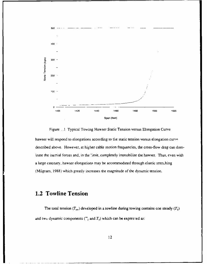
elongation. One aspect of this non-linear behavior is shown by the hawser's static tension
versus elongation curve (figure 1.1). At low mean tension levels, below the "knuckle" on the
curve, the towing hawser has a large catenary shape and acts like a damped spring. By
changing the geometry of its catenary, the hawser is able to absorb changes in elongation
with only slight variations in dynamic tension. However, at higher mean tension leels,
above the "knuckle," the hawser has little or no sag in its catenary shape and further hawser
extension is accommodated by elastic stretching which results in large dynamic tensions.
In addition to the above properties, the dynamics of submerged hawser tensions are
influenced by other non-linearities. Since towing hawser elongation constantly changes as
each ship moves, transverse motions are developed along the length of the hawser. The vis-
cous cross-flow drag force resulting from these motions can impact significantly on the
dynamic tension. The viscous cross-flow drag force (F) is a function of water density (p.),
length (1), local fluid velocity (U) and drag coefficient (CD(Re)) and can be approximated as:
F = /p2fU I U I CD(Re) (1.1)
Since the cross-flow drag force is proportional to the square of the local fluid velocity, the
effects of cross-flow drag are minimized at low cable motion frequencies and the towing
11
500
400 -
. 300-
CD0
W
I-
1_ 200-
- -oo- -- -
CO'
0- /
1400 1420 1440 1460 1480 1500 1520
Span (teet)
Figure .. 1 Typical Towing Hawser Static Tension versus Elongation Curve
hawser will respond to elongations according to the static tension versus elongation cur.'e
described above. However, at higher cable motion frequencies, the cross-flow drag can dom-
inate the inertial forces and, in the 'imit, completely immobilize the hawser. Thus, even with
a large catenary, hawser elongations may be accommodated through elastic stretching
(Milgram, 1988) which greatly increases the magnitude of the dynamic tension.
1.2 Towline Tension
The total tension (T,o,) developed in a towline during towing contains one steady (T,)
and twu dynamic components (, and T3) which can be expres-,ed as:
12

To, = T, + T, + T., (1.2)
The steady component of the towline tension (T,) has three distinct parts; the steady
tow resistance (R,), the hydrodynamic drag on the towline (R .,..), and the vertical component
of the wire weight (T,) and can be expressed as:
T. = +(R, +R,,)2 + T (1.3)
The steady tow resistance (R,) is a function of hydrodynamic hull resistance, hydrodynamic
propeller resistance, wind resistance, and sea state resistance. Except for the sea state
resistance at slow speeds, well established analytical methods exist for accurate prediction of
this component of tension. The hydrodynamic resistance of towline (R.,,) is a function of
the size, length, and geometric shape of the towline which are dependent on the specific tug
and the actual towing speed. Estimates of R.,,, for all towlines in use by the U.S. Navy are
presented in the U.S. Nays Towing Manual (1988). The vertical component of the towline
tension (T,) represents the weight of the towline forward of the catenary point and can be
approximated by the in-water weight of one half the scope of the towing hawser.
The dynamic tensions developed in a towline are comprised of low frequency and fast
dynamic tensions. The low frequency component of towline tension (T2) is caused by both
slowly-varying surge motions and "side slip." The added resistance of the towline creates an
exciting force on the two ships which exhibits a low frequency behavior due to its quadratic
dependence on the wave amplitude. "Side slip" refers to a special form of yawing motion
that is commonly experienced while towing in which the towed vessel slowly swings from
side-to-side relative to the centerline of the tug. This is a low frequency term because the
period of these motions is on the order of minutes. The fast dynamic tension component (T3)
is the result of wave induced seakeeping motions of both vessels. It is a random process with
13
typical periods of 4 to 30 seconds. For extreme tension calculations, T- can be the singularly
most important component of the towline tension as its magnitude can be larger than all other
components combined. Although most shipboard sensors are able to monitor the steady state
towline tension (T,), the two dynamic components (T2 and T3) are not easily measured
because of their rapidly changing nature. The main focus of this investigation will the be
measurement of T. and T and the factors that influence them.
1.3 Prediction of Towing Hawser Tension
Since hawser elongation is a function of ship motions, seakeeping theory must be
applied to determine the resulting tension in the towing hawser. The well established five
degree of freedom (DOF) strip-theory of Salvenson, Tuck, and Faltensen (1970) has been
incorporated into the MIT Five DOF Seakeeping Program (Loukakis, 1970) which computes
the hydrodynamic coefficients and wave forces for sway, heave, pitch, roll, and yaw. How-
ever, surge must be included in this analysis because it is the dominant ship motion influenc-
ing hawser extension.
The exciting force, added mass, and damping in surge for both vessels are evaluated
using the method proposed by Anagnostou (1987). By assuming that each vessel is only
excited by the undisturbed incident wave potential, the Froude-Krylov approximation is used
to obtain the wave exciting surge force. Surge added mass is approximated as five percent of
the actual displacement of the ship. The surge damping coefficients are evaluated as the
slope of the resistance curve at the towing speed with provis-ons made to account for propel-
ler damping of the tug. Surge can now be coupled with the five DOF system to form a com-
plete six DOF expression for the motions of each vessel. To analyze the entire towing
14
system, the motions of each ship must be coupled together to form a single 12 DOF system.
However, the complete towing system model must also account for the influence that
the towline tension has on motions of the two ships. This requires a coupling of the tension
in all 12 DOF. Since ship motions are influenced by towline tension and towline tension is a
function of cable elongation, the towing problem becomes a 12 DOF non-linear feedback
system. To solve this problem. the method of equivalent linearization has been adopted
(Frimm, 1987). This is a valid approximation because the forces and moments on the ship
due to the towline are considered small in comparison to the hydrodynamic and inertial
forces. The resulting ship motion response can then be used to compute the towline tension
extremes using the full non-linear methods.
Analysis of the non-linear behavior of towline tension is based on a set of governing
towline equations. They can be expressed as follows (Triantafyllou, 1987):
m -I= (T +)C a+-~ L b-q q Ta (1.4)
with
T-! ' qds +j fo(-s)jdS] (1.5)
where:
m = cable mass per unit length
w = cable weight per unit length
q = normal motion along cable
T = static tension
t = dynamic tensionwL
a - = catenary stiffness
s = Lagrangian coordinate along the cable
b = pCDL = sectional drag force
15

p, = water density
CD = cable sectional drag coefficient
D = cable diameter
E = Young's modulus of the cable
A = cross-sectional area of the cable
p = tangential motion along cable
L = cable length
By applying the Galerkin method with sinusoids as basis functions and Newmark's time
integration scheme, these equations will provide a series of time simulations of tension.
However, since these equations do not provide a closed-form relationship between the haw-
ser tension and the movement of the endpoints of the hawser, they cannot be used directly for
the prediction of tension extremes. Instead, Frimm (1987) proposed a "Numerical Towline
Model" to discretely express the non-linear towline tension as a function of cable elongation
( ) and its time derivative ( ). This model provides a polynomial approximation for the
non-linear towline tension which can be expressed as:
3 3 + m+n<3T NL( , 4) = Y". 7- a,.(t(t)t) .W (1.6)m,-o- -0 i(m, n) * (0, 0)
The coefficients of this equality are determined by minimizing the root mean square error
between the numerical model and the time simulations generated by the cable governing
equations.
By adopting the method of equivalent linearization for calculating ship motions, the
non-linear towline tension is approximated by a spring constant (k..) and a damping constant
(bq) and expressed as:
16

t( .A ) kq4(t)+ b,q(t) (1.7)
The fundamental requirement in applying the method of equivalent linearization is that both
the non-linear and equivalently linearized systems have the same cross-correlation function.
This requires that:
3 3k,E [i(t)r(t +.,)] +beqE[ (t)4(t +at)] = .X a E[ M(t)A(t)(t + T)] (1.8)
m-On-O
The statistics of this elongation response are:
E[=2(t)] Rk(0) = mo (1.9)
E(04(t)= d 2R4(,t) = 2 (1.10)
The cable spring and damping coefficients can now be expressed in terms of the coefficients
of the polynomial tension model (Frimm, 1987):
kq = a10+3a 3Mmo +a 12mk (1.11)
b, = a0;+3ao3 2 +a2m (1.12)
The equivalently linearized tension represents the "best" approximation to the non-
linear tension in the "mean square sense." In other words, the model is optimized for the
hawser tensions caused by cable extensions of the order of its RMS (root mean square) value.
Thus, extreme tensions are poorly approximated. To properly evaluate extreme tensions, the
fully non-linear numerical model (Frimm, 1987) must be used.
17

1.4 Planned Experiments
The analytical models described above have been adopted by the U.S. Navy as the
technical basis for the prediction of dynamic towline loadings in the U.S. Navy Towing Man-
ual (1988). Although it represents the most advanced theory currently available, it has not
been validated by full-scale experiments at sea. The focus of this study will be the planning
of a field test to assess the accuracy and applicability of these methods. Confirming the
validity of these analytical models will provide greater faith in the prediction of extreme ten-
sions. This will not only help to improve towing safety and give operators greater confidence
to tow at higher speeds when predictions for extreme tensions are low but perhaps allow also
allow for a reduction in the traditional factors of safety used in open ocean towing.
18

Chapter Two
Planning the Experiment
2.1 System Design Criteria
To obtain the necessary data for analysis of towline tensions, simultaneous measure-
ment at two separate locations (the tug and tow) will be required. The tug will be designated
as the primary data collection site. All data collected on the tow will be relayed to the tug on
a real-time basis using telemetry.
The selection of equipment for this experiment will be based on compactness, reliabil-
ity, accuracy, self sufficiency, and having sufficient resolution to provide significant data
even when sea conditions are calm. Every attempt to minimize interference with, or
dependence upon, installed shipboard systems must be made. Although electrical power is
generally readily available on the tug, space is always at a premium which requires the use of
compact equipment. The portability of test equipment is of prime concern: it should be
designed for quick, drop-in installation and be small enough to allow handling up and down
ladders. The equipment must be completely self-contained and operationally tested before
installing it on either vessel.
If the tow is to be manned, and both power and space are available, the ideal setup
would be to install a laboratory type data acquisition system with an operator in direct com-
19

munication with the primary data acquisition station operator. However, since it is standard
practice for the U.S. Navy to tow vessels unmanned, some form of self-powering, such as
batteries or a portable generator, will be required on the tow to operate the electronic equip-
ment. In previous experiments (Campman & DeBord, 1985), one of the major causes for
failure was power supply problems. Therefore, hardware designed to operate from batteries
must either draw so little current that the battery life span will far exceed the time limit of the
experiment or it must be able to power up and down to conserve power whenever measure-
ments are not being made. In addition, a means of recharging the batteries during the experi-
ment must be provided.
2.2 Data Transmission
Data transmission can be either via analog (FM) or digital telemetry. It is imperative
that the transmission system not increase the relative error of the measurements above speci-
fied limits. Radio interference of data transmission has been a severe handicap in previous
experiments (DeBord, Purl, Mlady, Wisch, & Zahn, 1987). Analog systems offer the
advantage that raw data can be transmitted and stored. This means that post-voyage analysis
is not limited by sampling system constraints. However, analog telemetry is very frequency
sensitive and the slightest drift in frequency will translate directly into measurement error.
Digital transmission systems, on the other hand, are much more tolerant to finite changes in
frequency and signal levels and data can be multiplexed for a large number of channels at
low power consumption. However, digital transmission systems are limited by bandwidth
constraints. Therefore, since neither system shows a dominant superiority over the other, the
final selection of transmission system type should be based primarily on the availability of
resources.
20

2.3 Data Filtering
Data filtering is required to reject the high frequency components of unwanted noise
which can introduce distortion or aliasing into the recorded data. Aliasing can be avoided by
ensuring that the sampling interval is small enough that the maximum frequency component
of the desired signal is less than the upper cutoff frequency.
The first step in determining the upper cutoff, or Nyquist, frequency is to select a sam-
pling interval. It is important to ensure that the Nyquist frequency is high enough to cover
the full frequency range of the continuous time series. Since this requires some prior
knowledge of the frequency content of the data to be sampled, analytical models can be used
to predict frequency spectrums. The Nyquist frequency (f,) is then determined by the selec-
tion of the sampling interval (&) and can be expressed as:
1f. = -1(2.1)
All data is to be attenuated as needed to provide a ±10 volt input to the data acquisition
system. This will allow for uniform resolution sensitivity for each parameter being mea-
sured. All signals should have identical filtering to avoid introducing relative phase shifts
between data channels.
2.4 Data Recording
All data collected at the main data acquisition site on the tug shall be in digitized form
and recorded on diskettes compatible with the IBM-PC standard. This will allow playback
and complete post-voyage analysis. A redundancy in the recording of all measurements is
21

desirable and considered necessan' to provide a measure of safety should data transmission
problems occur. Therefore, all data measurements on the tow are to be digitized and
recorded on a personal computer while being telemetered. The data acquisition equipment
should allow active monitoring of data during the designated test interval.
The real-time measurement and recording of data must be dynamic in nature: instru-
ment response times and sampling intervals must be fast in comparison to the motions of the
tug, tow, and towing hawser. Digital data is to have 12-bit accuracy and signal amplification
is to be used such that the allowed error corresponds to at most three bits.
Data acquisition through all channels must take place in a "burst mode" with one burst
occurring each sample period. The maximum time skew between "adjacent" channels is to
be 30 microseconds. Since each burst of data will take about one millisecond, the data acqui-
sition system will be inactive for most of the time. The timing accuracy in the data acquisi-
tion and recording system is to be within one part in 10,000. Therefore, all data should be
recorded on a single device to prevent possible timing errors associated with recording on
multiple devices. The system time at the start of each data acquisition "burst" shall be
recorded along with the data from that "burst."
2.5 Data Processing
A lthough most data processing can be accomplished upon completion of the experi-
ment, some immediate analysis must be done to determine if the data recorded is correct and
if the results are meaningful. This will require that extensive preparations be done before the
experiment so that analytical predictions are available for all scenarios anticipated during the
22

actual data recording. During the experiment, a computer program must be able to provide
average values, power density spectrum for all dynamic measurements, and provide a com-
parison of measured statistics to the theoretical predictions.
2.6 Test Location
The selection of the most favorable location to conduct the towing experiment is
dependent upon several key aspects; the availability of a naval towing asset, the availability
of sufficiently large enough vessel to be towed, and the prevailing weather patterns.
Although U.S. Navy salvage tugs operate worldwide, they are limited in number as shown in
Appendix A. They are concentrated into three main "home ports"; Little Creek, Virginia,
San Diego, California, and Pearl Harbor, Hawaii. The availability of one of these vessels to
support this experiment is contingent upon their operational schedules as dictated by their
local fleet commanders. Generally, these vessels are available only for regularly scheduled
tows which would mean that the experiment would have to be conducted on a "tow of oppor-
tunity" basis. There are several serious drawbacks to using a "tow of opportunity" vice a
"dedicated tow." The installation and conduct of the towing experiment would be of
secondary importance and most likely be on a "not-to-interfere" basis. This would place
great restrictions on the ability of obtaining sufficient (" .ta to examine all factors influencing
tension extremes. Since open ocean tows generally last thirty days or longer, there is also the
problem of how to disembark the experimenters and equipment at sea upon completion of the
experiment without requiring them to remain on the tug for the entire voyage.
The availability of a "towed" vessel that is large enough that measurable dynamic ten-
sions will result is even more difficult to plan. Although the prime choice would be to use an
23

operational ship. the availability and scheduling of such a ship for a minimum of two weeks
(to allow time for installation, testing, and demobilization) is very unlikely and cost prohibi-
tive. A more realistic alternative would involve the use of a barge or decommissioned ship.
Using a barge is the least preferred method as the dynamics of its motions could differ
greatly from an naval surface combatant. The most likely source of obtaining a vessel to tow
would be a decommissioned ship: either incident to a transfer to inactive status or one pres-
ently in "moth balls."
Local weather conditions will play a significant role in the outcome of the experiment.
In normal tow operations. it is highly desirable to minimize dynamic loadings on the hawser
by avoiding weather extremes. However, the opposite is true with this experiment as some
extreme weather influences are required in order to obtain a larger range of dynamic tension
extremes. The two most significant environmental factors influencing this experiment are
the wind speed and "fetch," the horizontal distance over which the wind blows. As will be
shown in a sensitivity analysis (chapter 4), relative wind speeds greater than 15 knots are
needed to generate measurable dynamic tensions. To identify possible test location sites that
meet this requirement, a review of historical synoptic weather patterns along the coastline of
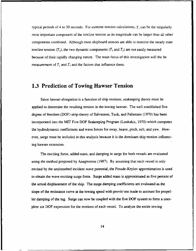
the United States was undertaken. Figure 2.1 provides the seasonal variation of the mean
wind speeds for the six most logical locations. It should be noted that these are only mean
wind speeds and for exact probabilistic determination, their actual frequency distribution
should be used. However, the mean values are adequate for comparison of the relative supe-
riority of the one site over another.
Oahu, Hawaii presents the most favorable location for the experiment because of its
high mean wind speeds for the majority of the year. In addition, since it is an island, fetch
lengths should be very large and hence larger wave heights can be anticipated. Conducting
the experiment at several different locations around the isiand would allow measurement of
24

14
13 -
12 -"
i1 8 - ."- "N'I6 AS~-~
7 -- /
"
Z 9-
8-
77
5JAN FEB MAR APR MAY JUN JUL AUG SEP OCT NOV DEC
SAN DIEGO 0 SEATTLE 7 CHAR ESTON
SAN FRANCISCO L. OAHU X NORFOLK
Figure 2.] Mean Wind Speeds of Selected Sites
dynamic tensions in different sea states since the fetch length on the lee of the island would
be significantly less than that of the windward side. Although the Norfolk area has higher
mean wind speeds in January through March, the prevailing wind direction at that time of
year is from the southwest which would tend to minimize the fetch length. Therefore, strictly
from an environmental viewpoint, the most favorable time period for this experiment would
be June through August around Hawaii. However, because of time constraints imposed by
the deadline of this thesis, an earlier date must be used. Even though the trade winds of
Hawaii would not be at their peak, they are considered sufficiently strong to provide measur-
able dynamic tensions.
25

Chapter Three
Parameters to be Measured
3.1 Towline Tension
3.1.1 Background
The total tension developed in a towline while towing contains both steady and
dynamic components. The installed shipboard sensors on a towing ship are designed to mea-
sure only the mean steady tension. Due to their rapidly changing nature, dynamic tensions
are not normally measured but are simply accounted for by applying factors of safety to the
towline design. However, in order to validate analytical predictions, both the steady and
dynamic tension components must be accurately measured.
3.1.2 Sensor
During normal towing operations, a visual display of the towline tension, as measured
from an installed tensiometer on the towing machine, is maintained on the tug. However,
this sensor should not be used for the towing experiment because neither its calibration nor
sensitivity to dynamic loading can be properly guaranteed and confirmned before the experi-
ment without extensive testing. Time permitting, a bollard pull test could be conducted to
compare the tension in the load cell to that of the installed tensiometer. However, the
26
logistics of adding this test would significantly increase the complexity of this experiment
and delay the completion of the seakeeping test. Therefore, stand alone tension sensing
devices should be used; one on the tug and one at the tow end of the hawser. Typical sensors
used for this type of application are tension links containing internally mounted strain gage
bridge circuits which produce an output voltage proportional to the amount of strain (tension)
developed on the device.
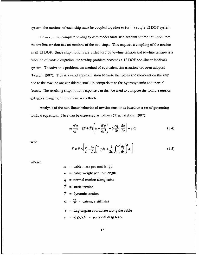
Measurement of the tension at the tug end will be accomplished using a tension link
attached directly to the hawser using a carpenter stopper as shown in figure 3.1. The tension
link will be secured to a deck padeye on the fantail of the tug using a wire rope pendant.
Measurement of tension at the tow end will be accomplished using a waterproof, load sens-
ing clevis pin type tension link which will directly replace one of the standard shackling bolts
connecting the towing hawser to the towing bridle as shown in figures 3.2 and 3.3. The load
sensing clevis pin employs internally mounted strain gages positioned on a neutral axis plane
relative to one specific plane of pin loading. This allows the pin to produce an electrical sig-
nal proportional to axial loading.
3.1.3 Calibration
Calibration of the load cells requires laboratory testing using an extensometer or sim-
lar device capable of produciig large tensions. As both load cells will be factory calibrated
before the experiment, no on-site calibration is necessary. Since the towing load will be
taken up by the load cell, the ship's installed tensiometer will be inoperative during testing
and cannot be used as a redundant source. However, comparison of the readings from both
ends of the hawser would help to provide an indication if one should malfunction.
27

DE:K< ArEE
SAFET SHAZKLE VIRE PENDANT
TENSION LINK
SA--[TY S -ACK-7
CAQPENlTP STOOPER -
YE,---.--TW HAWSER
Figure 3.1 Tension Measuring Configuration on the Tug
Clevis Pin
-zIIIIzzzzWire Pendant --
Flounder Plate
Figure 3.2 Tension Sensing Clevis Pin Instalation
28

CHAiN BPRD-E
-DETACHABLE LINK
-PLATE SHACKLE
F'LOLNZR P_ ATE
ZLEVIS PIN
WRE PE' DAN-
PLATE SHACKLE
~-DETACHABLE LINK
CHAIN OENDAN"
Figure 3.3 Tension Measuring Configuration on the Tow
3.2 Ship Motions
3.2.1 Background
The motions of a ship at sea in a confused, three dimensional sea are very complex but
can be broken down into six degrees of freedom relative to three mutually perpendicular
coordinate axes. The hydrostatic frame of reference used to describe these motions is an ort-
hogonal, right-handed, "earth fixed" coordinate system (Xo,Yo,Zo) where X, is the direction
of mean forward ship motion, Y. is positive to port, and Z, is positive vertically up. The
angular motions follow the right-hand-rule convention as shown in figure 3.4.
29

HeaveZo Surge
Sway Pitch YwX
/. Roll
Figure 3.4 Earth Fixed Coordinate System
The motions experienced by a floating body include the three rectilinear motions of
surge (x), sway (y), and heave (z) and the three angular motions of roll ((p), pitch (0), and
yaw (xV) which are defined as follows (Comstock, 1967):
Surge: the longitudinal component of dynamic motion that is hori-
zontal in the direction of forward ship motion parallel to the
XoYo-plane, positive forward.
Sway: the transverse component of dynamic motion that is horizon-
tal along the Y-axis and parallel to the XoYo-plane, positive to
port.
Heave: the vertical component of dynamic motion that is perpendicu-
lar to XY-plane, positive up.
30

Roll: the transverse oscillatory rotation about the ship's longitudi-
nal axis measured from the vertical XZ.- plane to the Z-axis,
positive with the starboard side down.
Pitch: the longitudinal oscillatory rotation about the ship's trans-
verse axis measured from the horizontal X,,Yo-plane to the
X-axis, positive with the bow down.
Yaw: the angular oscillatory rotation about the ship's vertical axis
measured from the vertical X0Z-plane to the X-axis, positive
with the bow to port.
Any or all of these motions may coexist at the same time and the resulting superposi-
tion of motions is complex and often difficult to describe. Since each ship operates in a six
DOF domain, complete analysis of the motion of the towing system will require the solution
of 12 simultaneous equations.
During the experiment, a complete time history record of the motions of both the tug
and tow in all six DOF is required. Measurements will be made using motion detection
devices that contain both accelerometers and gyroscopes. Since the recorded data must be
referenced to the earth fixed coordinate system to be consistent with the analytical model, the
use of gyro stabilized accelerometers is preferred. However, uncompensated accelerometers
can be used if corrections are applied to translate their ship referenced output signals into
earth referenced coordinates. Similarly, corrections must be made to the account for the fact
that gravitational acceleration varies on the mean axis of non-stabilized accelerometers.
3.2.2 Sensors
For this experiment, two six DOF motion sensing packages, each containing a vertical
referenced gyro, capable of measuring pitch and roll, and six servo accelerometers, will be
used. The main unit, consisting of a gyro and three accelerometers, will be mounted at the
31
ship's Center of Gravity (CG). The three other servo accelerometers will be packaged in sep-
arate containers and located at known distances from the main unit. They will be capable of
measuring angular accelerations directly which will eliminate the need to differentiate the
gyro angles to obtain the angular motions. Since the chosen translational accelerometers are
not gyro-stabilized, a correction must be applied through software during data recording.
3.2.3 Calibration
All accelerometers will be factory calibrated before installation. Before beginning the
experiment, the operational status of all accelerometers must be verified in a complete end-
to-end dry run conducted in a laboratory environment. During installation, the signal from
each transducer should be verified by manually rotating the sensor to confirm the validity of
the output signal. Care must be taken to ensure that the sensors are not placed in a locale that
is influenced by structural vibrations which could invalidate their measurements.
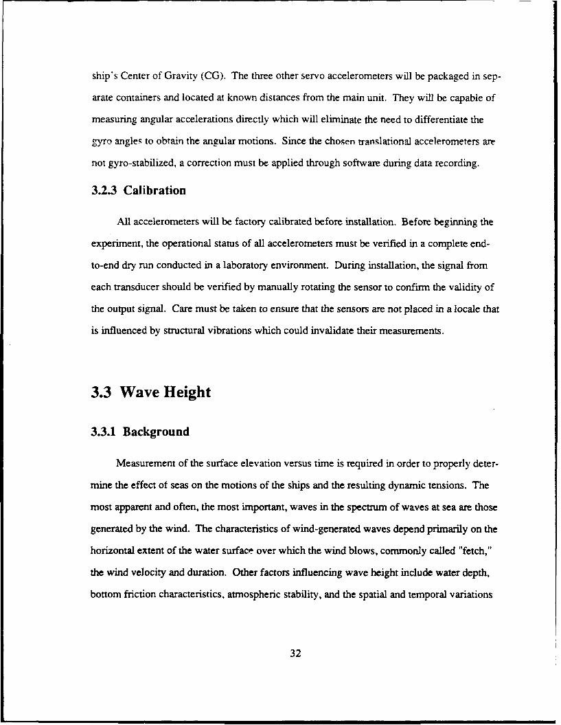
3.3 Wave Height
3.3.1 Background
Measurement of the surface elevation versus time is required in order to properly deter-
mine the effect of seas on the motions of the ships and the resulting dynamic tensions. The
most apparent and often, the most important, waves in the spectrum of waves at sea are those
generated by the wind. The characteristics of wind-generated waves depend primarily on the
horizontal extent of the water surface over which the wind blows, commonly called "fetch,"
the wind velocity and duration. Other factors influencing wave height include water depth,
bottom friction characteristics, atmospheric stability, and the spatial and temporal variations
32

in the wind field during wave generation.
Although the wind speed is perhaps the most significant aspect in determining the
height of waves, strong winds do not generate high waves instantaneously but require a con-
siderable period to do so. For wind blowing for a given duration or over a certain fetch dis-
tance, there is a fixed limit to which the average wave height, period and spectral energy will
grow. At this limiting condition, the rate of energy input from the wind to the waves is
balanced by the rate of wave energy dissipation due to wave breaking and turbulence. This
condition, known as a fully developed sea, is used for the development of many standardized
wind wave spectra including the Pierson-Moskowitz spectrum.
3.3.2 Sensor
The measurement of wave height spectra can be accomplished using either a wave
measuring buoy or an installed shipbome sensor. Since the motions of the ship will disturb
the local wave pattern, the preferred method is to use a stand-alone measuring buoy located a
short distance away from the ship. However, this places great restrictions on the maneuver-
ability of the towing ships as the experiment must be conducted in the vicinity of the buoy.
The National Oceanic and Atmospheric Administration (NOAA) maintains a series of
permanently moored, self-contained buoys strategically located along all coastlines of the
United States which could be used for this purpose. Unfortunately, data from an individual
NOAA buoy is not available on a real-time basis. These buoys transmit specially coded
information directly to the National Data Buoy Center (NDBC) in Bay St. Louis, Mississippi
via satellite. This results in a minimum of a three week delay in obtaining data on a specific
buoy from NDBC. The other major drawback in using a NOAA buoy is that the operational
status of one of these buoys at some date in the future cannot be guaranteed beforehand.
33

Since the planning of a towing experiment takes months of coordination between different
organizations, an alternate and more reliable source of measurement is required in case the
NOAA buoy is not operational at the time of the experiment.
One attractive alternative is to deploy a portable buoy, capable of measuring low fre-
quency waves, directly from the ship. Although this method allows greater freedom in the
selection of the location to conduct the experiment, it presents its own set of restrictions. The
availability of a support craft, which is needed to deploy and relocate the buoy between data
collection runs, is very dependent upon the local sea conditions. This could significantly
impact on the conduct of the experiment especially considering that it is highly desirable to
conduct the experiment in areas of higher sea states. Also, the transmission of data from the
portable buoy to the data acquisition system requires either additional telemetry gear or pro-
viding a means to record the data locally on tape recorders and then manually retrieving and
entering the data into the data acquisition computer.
A second alternative, which presents fewer restrictions on the conduct of the experi-
ment, is a non-contacting shipborne wave measuring device. This type of sensor must have a
wide dynamic response as low frequency waves have small accelerations which must be
detected in the presence of large, high frequency ship accelerations. One type of shipborne
measuring device is a portable microwave radar. The unit records the surface velocity by
measuring the Doppler shift in radar transmissions bounced vertically off the sea surface.
However, the influence of ship motions on the measured data is now a problem. The velocity
of the radar is the lesser difficulty since it can be accounted for by integrating the accelera-
tion of the instrument.
As a ship heaves and pitches, it radiates energy into the water in the form of waves.
Waves are also generated as the ship travels through the water. Therefore, unless an on-site
calibration procedure is performed, the influence of these ship generated waves will severely
34

corrupt all wave height measurements. This has been confirmed by Sellars (1967) who
found large variations in frequency response due to the influence of the ship's hull on the
wave height measurements. In addition to individual hull characteristics, the calibration of
these devices is a function of wave encounter frequency, relative heading of the waves, ship
speed and the pitching motions of the ship.
The sensor to be used in this experiment, a TSK remote wave height meter, contains an
internal, compensated linear accelerometer which decouples the pitching motions of the ship.
To minimize the influence of ship generated waves on the actual wave system, the unit will
be mounted on a post extending forward of the bow of the ship. For bow mounted instru-
ments, Sellars found the optimum location to minimize variations in the frequency response
of the unit to be at a distance of four percent of the length of the ship.
3.3.3 Calibration
The conventional method for evaluation of the performance of a wave measuring sen-
sor is to compare its output with other wave measuring systems. This will iivolve recording
data in the local vicinity of the reference wave height measuring system while steaming at
various speeds on different courses relative to the waves. Then, by comparing the measured
data with the actual wave height as recorded by the reference system, a calibration matrix can
be determined for the specific hull form. For this experiment, recorded data can be compared
to NOAA buoy data.
Although the accomplishment of this calibration procedure will extend the time
required for the experiment, it is considered essential. Since the waves generated by the tow
can be considered to have no influence on the tug, only the tug is required to perform this
35

procedure. Since there is no real-time feedback from a NOAA buoy, this calibration proce-
dure can be conducted independently from the experiment. However, since the installation
of instrumentation is costly and time consuming, it would be more cost effective to conduct
these calibration procedures as part of the experiment.
3.4 Wind Speed and Direction
3.4.1 Background
The most significant aspect in wind measurement is the positioning of the sensor. The
wrong location can lead to errors large enough to far overshadow any loss in accuracy
because of less-than-perfect calibration. A unique and deterministic relationship between
calibration factor, wind direction, and gradient does exist and it can only be accurately deter-
mined in a wind tunnel experiment which far exceeds the scope of this experiment. How-
ever, there are some general guidelines that can be followed to minimize installation errors.
The anemometer and wind vane unit should be placed as high as possible on one of the
tug's masts in a position that provides unobstructed wind from all directions. The unit must
be above the turbulent separated region near the top of the superstructure or significant errors
will result. Since these instruments only measure on the horizontal plane, out-of-plane flows
affect both wind speed and direction measurements. An up-wash flow is caused by the
superstructure obstructing the wind's flow pattern. Durgin (1975) found that the sensitivity
of wind direction measurements to be in error by as much as 10 degrees with a 35 degree
up-wash angle. He also found that the wind speed measurements (Vi,,d) differed from the
actual wind speed (V,,) by the square of the cosine of the up-wash angle (f3) as given by:
= v.,, cos2( ) (3.1)
36

Therefore, except for small angles (less than 10 degrees), it is very important to know the
up-wash angle in order to properly correct both wind speed and direction measurements.
However, since the up-wash angle is highly sensitive to wind direction and wind tunnel tests
are required to calculate it, the best way to minimize its effects is to install the unit as high as
possible on the ship's mast, preferably near one of the existing wind sensors.
3.4.2 Sensor
To avoid interference with or dependence on shipboard sensors, the preferred method is
to use a dedicated instrument rather than rely on the signal from the tug's wind anemometer
and wind vane. To minimize the amount of data telemetered between the two vessels, the tug
is the preferred vessel on which to install the sensor.
For wind speed measurement, the most obvious choice is either the classical propeller
or cup type anemometer because of their proven reliability at sea. Wind speed transducers
are generally AC generators which have spin rates proportional to wind speed. Selection of
the specific unit should be based on the following design characteristics: threshold velocity,
the velocity at which the unit first starts to spin and at which the unit stops spinning as wind
velocity decreases; friction velocity, the velocity by which the true calibration curve is dis-
placed from the ideal one because of bearing friction; and dynamic response, listed as a dis-
tance constant.
For wind direction measurement, two types of wind vanes are most commonly used;
synchro and potentiometer. Both are influenced by the interaction between the wind vane
and anemometer. Propeller type anemometers induce errors in direction measurements due
to rotating flow behind the propeller. Cup type wind vanes are usually mounted above the
37

anemometer on a post which passes through the plane of the cups. Thus, for certain direc-
tions, the cups pass through the wake of the supporting vane which introduces errors up to
ten percent in their direction readings.
3.4.3 Calibration
Calibration of wind anemometer can be checked by removing the propeller and rotating
the shaft of the unit at a known speed. The two parameters needed to describe the calibration
of a cup anemometer Z-e the calibration slope (k) and friction velocity (Vf). A linear relation-
ship exists between the actual wind speed (V,,) and shaft rotation which can be expressed as
follows:
v = Vf + k(rpm) (3.2)
Although the calibration slope of a given instrument is generally a constant, its friction veloc-
ity often increases during field use. Because of the short duration of this experiment, the
known values from the initial factory calibration can be assumed to remain constant during
the experiment. A post calibration can be conducted upon completion of the experiment to
verify this.
The wind vane transducer uses internal potentiometers to measure the wind direction
relative to a reference direction, usually true north. Calibration consists of manually training
the unit and adjusting the potentiometer until zero ohms are output when the vane passes
through the designated reference direction. During actual testing, comparison with the
readings from the installed shipboard sensors can be used as a check. Since NOAA buoys
record wind speed in addition to wave height, the calibration of the wind instrument and
influence of up-wash angle can be checked during the wave height sensor calibration proce-
dures described in the previous section.
38

3.5 Ship's Speed
3.5.1 Background
The standard installed shipboard instrument to measure speed and distance traveled
through the water is called a "log." The two most common types are the electromagnetic
speed log and the pressure tube Pitot log. The electromagnetic speed log uses a solenoid and
sensors contained in a housing mounted flush with the bottom of the hull. It operates on
Faraday's law of electromagnetic induction; the water moving past the hull in the magnetic
field generated by the solenoid induces an electromotive force that is directly proportional to
the speed of the ship. The Pitot log, on the other hand, consists of a rodmeter or Pitot tube
that extending below hull of the ship. The difference between the dynamic and static pres-
sure is translated into deflection of a diaphragm which is proportional to the square of the
ship's velocity. The distance traveled can be computed by electronically integrating the
measured analog velocity signal.
Since the operational status and accuracy of the installed unit on the tug is uncertain
and to avoid disrupting ship operations, it is preferable to provide a stand alone unit. Since
the installation of a shipboard log is very complex and well beyond the scope of this experi-
ment, an alternative method must be used. Possible choices include non-contacting sensors,
similar to the Doppler radar used to measure the wave height, or to compute the ship's speed
from navigational plots. Based both on the available resources and success in previous
experiments, the method of choice for this experiment will be to use a portable LORAN C
receiver to record the ship's speed.
39

LORAN, which stands for "long range navigation," is an electronic system using shore
based radio transmitters and shipboard receivers to allow mariners to determine their position
at sea. It is a low frequency (100 kHz fundamen:al carrier frequency with 20 kHz band-
width) pulsed hyperbolic navigation system operated by the U.S. Coast Guard. A hyperl-olic
line of position is derived from the difference in arrival time of pulses from two transmitting
stations. The position of a ship can be computed by interpolating between hyperbolic lines
on a LORAN C chart. Based on the time between successive fixes, the speed of the ship can
be computed.
3.5.2 Sensor
The portable LORAN C unit selected for this experiment belongs to the test sponsor,
NAVSEA OOC. It has been used successfully in previous experiments. It provides both a
digital readout of longitude and latitude, time, LORAN time differences (TD's), latitude and
longitude, speed over ground (SOG), course over ground (COG), and an indication of the
reliability of the LORAN data. Besides the digital display, the unit has an RS-232 output for
direct recording of information onto a file on a computer disk. The unit provides an average
reading of the SOG with an accuracy of 0.1 knot. The unit estimates the latitude and longi-
tude from the TD's using a mathematical conversion process that is accurate to within 0.25
nautical mile.
LORAN receivers generally do not update synchronously but rather, output a data
stream each time a new fix is computed. This occurs at regular intervals of 8 to 30 seconds
which is satisfactory for this experiment. The LORAN uses an averaging process between
successive fixes to compute the ship's speed. The interval time is user definable between six
seconds and seven minutes. Therefore, the longer the interval between updating, the more
accurate the data. Since the tug will be requested to maintain a constant course and sneed
40

during each test run, a record of the average speed during the test is satisfactory. This means
that the output from the LORAN can be recorded at a much slower rate than the other, more
time-sensitive, measurements.
3.5.3 Calibration
Since the LORAN C unit is fully self-contained and provides a comprehensive self test
upon powering up, no special calibration procedures are needed. After pierside installation,
the latitude and longitude readings on the unit can be verified with the vessel's known posi-
tion. During operation, the unit has several built in warning alarms to warn of poor data
quality. These include a low signal-to-noise ratio alarm, a cycle alarm to indicate when the
unit is not confident that it is tracking the correct ten microsecond cycle of the LORAN
pulse, and a blink alarm to warn that the LORAN transmitter is having technical difficulties.
Under normal operating conditions, a visual display shows when the unit is receiving a TD in
the normal tracking mode. In addition to these warning indicators, all data output can be
compared to navigational plot maintained by the bridge team of the tug using the ship,
installed sensors.
3.6 Heading
3.6.1 Background
To define the geometry of the towing configuration, a record of the time-varying head-
ings of both the tug and the tow with respect to true north is required. This will require the
use of a magnetic compass. Since magnetic compasses, whether mechanical or electronic,
are sensitive to magnetic fields, any magnetic disturbance near a compass will deflect it from
41

the proper reading. Therefore, provisions must be made to compensate for both the perma-
nent and induced magnetism of the ship. There are two man corrections that must be
applied to magnetic compass readings to obtain the true heading; deviation and variation.
Deviation accounts for both the permanent and induced magnetic properties of steel and iron
ships. Variation accounts for the fact that the earth's magnetic lines of force do not coincide
directly with the geographical meridians.
Permanent magnetism is the result of inherent magnetic properties of steel and hard
iron used in construction of the ship. Welding, bending, and twisting of steel during fabrica-
tion provides stress which magnetize the ship. Subsequent vibrations by machinery and
shocks induced by the sea produce stresses which can alter the magnetic state of a ship.
Thus, induced magnetism is dynamic in nature as it varies constantly depending on the loca-
tion and heading of the ship and the stress the ship has been subjected to.
3.6.2 Sensor
The selection of the sensor to accomplish this is guided by power requirements, the
effects of magnetic influence from the metal hull, ease of installment, and required calibra-
tion procedures. To avoid interference with ship w rations, it is preferable to use a dedi-
cated instrument rather than rely on the tug's installed gyroscope. Since the installed sensors
on the tow will not be operational, a stand-alone instrument must be used.
The best instrument for this experiment is an electronic compass, also known as a flux
gate compass. It consists of a saturated core around which two coils with opposing polarities
are wound. In the absence of an external magnetic field, the coils are balanced with no out-
put voltage. As the ship moves, the magnetic field of the earth changes with respect to the
compass. This causes a reinforcing of the field of one coil and a detraction from the other.
This unbalanced condition causes the circuit to produce a voltage that is proportional to the
42

ambient magnetic field. The flux gate compass is lightweight, has no moving parts, exhibits
excellent transient response characteristics, and is insensitive to vibrational disturbances
which makes it ideally suited for marine applications. It can be powered by either 12(,eVAC
or with nickel-cadmium batteries.
3.6.3 Calibration
Preliminary compass adjustments can be accomplished pierside to minimize the effects
of the inherent magnetic properties of steel and hard iron used in construction of the ship.
However, since the induced magnetic signature of the ship is dynamic in nature and varies
depending on the ship's location and orientation with respect to the magnetic poles, final
compass corrections can only be accomplished at sea.
Magnetic compasses calibration is accomplished by comparison to a compass of known
deviation through a standard procedure known as "swinging the ship." This involves steam-
ing the ship on various magnetic headings and comparing the compass readings to a refer-
ence compass. For this experiment, calibration of the flux gate compasses will be
accomplished by steaming the ship in known reference directions and comparing the
measured heading with that of the ship's installed magnetic compass. By knowing the devi-
ation of the ship's magnetic compass, the deviation of the flux gate compasses can be com-
puted. Since the tow has no operational power, the tug's magnetic compass will be used as
the reference compass for calibration of both flux gate compasses. Simultaneous recordings
of the headings from both flux gate compasses and the tug's magnetic compass will be taken.
The reading from the tow will be obtained via telemetry on a real time basis. The average
from three attempts at each heading will provide a reasonable estimate of the deviation of
each flux gate compass for that heading. Although this will only be a "pseudo" calibration
procedure, it is accurate enough for purposes of this experiment as we are mainly interested
43

in the time-varying changes in the headings of both vessels while towing. To detect if the
tow has a steady yaw angle, which would s,-riously affect the calibration procedure, a contin-
uous measure of the angle between the centerline ob both ships must be maintained. This
can be accomplished using the installed flux gate compass on the laser range finder, which is
discussed in the following section.
3.7 Distance
3.7.1 Background
A measure of the time history of the separation between the tug and tow is required to
define the geometry of the towing configuration. The use of the tug's installed radar system
is unsatisfactory for several reasons; its dynamic response is unknown, radars have a "blind
spot" directly astern, and the desire to minimize dependance on shipboard sensors. Instead, a
stand-alone portable range finder capable of operating from an unstable and moving platform
should be used. Although this poses significant problems to conventional range finders, a
laser range finder, which uses very short measurement intervals, can easily accommodate an
unstable platform.
A laser range finder houses an internal electrical pulse generator that energizes a semi-
conductor laser diode which, acting as an optical transmitter, emits infrared light pulses.
Using optics, these pulses are concentrated and transmitted. The reflected signal from the
target passes through a reception lens and strikes a photo diode generating an electrical
reception signal. The range between vessels is computed based on the time between the
transmission and reception using a quartz-stabilized clock frequency. With a knowledge of
44
the exact location of both the laser and its reflector on each vessel, the actual distance
between the two ships at any given instant can be computed using trigonometric relation-
ships.
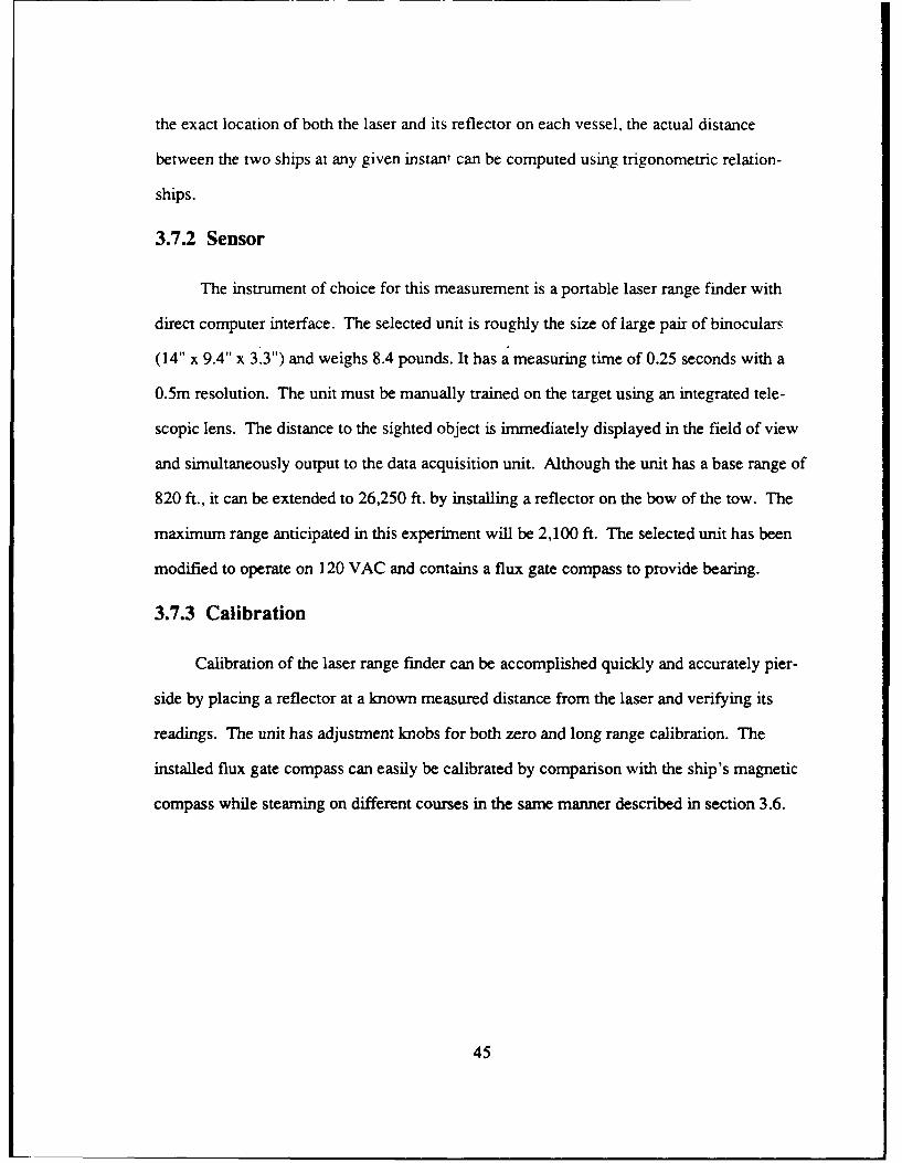
3.7.2 Sensor
The instrument of choice for this measurement is a portable laser range finder with
direct computer interface. The selected unit is roughly the size of large pair of binoculars
(14" x 9.4" x 3.3") and weighs 8.4 pounds. It has a measuring time of 0.25 seconds with a
0.5m resolution. The unit must be manually trained on the target using an integrated tele-
scopic lens. The distance to the sighted object is immediately displayed in the field of view
and simultaneously output to the data acquisition unit. Although the unit has a base range of
820 ft., it can be extended to 26,250 ft. by installing a reflector on the bow of the tow. The
maximum range anticipated in this experiment will be 2,100 ft. The selected unit has been
modified to operate on 120 VAC and contains a flux gate compass to provide bearing.
3.7.3 Calibration
Calibration of the laser range finder can be accomplished quickly and accurately pier-
side by placing a reflector at a known measured distance from the laser and verifying its
readings. The unit has adjustment knobs for both zero and long range calibration. The
installed flux gate compass can easily be calibrated by comparison with the ship's magnetic
compass while steaming on different courses in the same manner described in section 3.6.
45

3.8 Hawser Angles
3.8.1 Background
A measure of the relative heading, both vertically and horizontally, of the towline from
the centerline of both the tug and tow is required to properly define the geometry of the tow-
ing configuration. Since this parameter is not normally measured during towing operations,
no installed shipboard systems will be present. Because of the slow, time-varying nature of
"side slip," the measurement of this variable is simplified.
3.8.2 Sensor
The vertical and horizontal angles at each end of the hawser will be measured using
two spring-loaded, string-type potentiometers connected directly to the towing hawser.
Changes in the length of the string are translated directly into an electrical signal which can
recorded on the data acquisition unit.
3.8.3 Calibration
The accuracy of the string potentiometer is largely a function of correct positioning.
Although the hawser angles will be determined using trigonometric relations, it is vitally
important that the installation of the device be done correctly and with close tolerances.
46

Chapter Four
Sensitivity Analysis
4.1 Background
Current towing design and operational procedures are based strictly on the mean static
towline tension. Dynamic tensions are accounted for solely by applying factors of safety to
the static tension. Since both analytical predictions and full-scale towing experiments have
shown that the dynamic tensions can be the same order of magnitude as the mean tension, a
better understanding of the nature of dynamic tensions is needed. Although the static towline
tension is primarily a function of tug power and the tow resistance characteristics, the factors
influencing the dynamic tension are not as well defined. Using the equivalently linearized
theory, dynamic tensions are considered to be primarily a function of towline extension and
its time derivative (equation 1.6).
Although in normal towing operations it is highly desirable to minimize towline ten-
sions, during an instrumented validation experiment it is essential that there are measurable
differences between the mean and dynamic tension. To be able to preselect conditions in
which a higher range of dynamic tensions can be expected, a better understanding of the
parameters that influence towline extension is needed. This was done by performing a series
47
of time-domain computer simulations. By varying only a single parameter on each succes-
sive iteration, the individual effects of each parameter on the resulting dynamic tension were
identified.
Because towing operations are conducted at different hawser lengths and changing the
hawser scope is a simple process, five different lengths between 1000 and 2100 feet were
considered. To gain a better appreciation for the influence that sea conditions have on the
dynamic tension, four different sea states were simulated. To investigate the influence of
mean static tension, four mean tensions between 10 and 80 kips were simulated. Finally, to
assist in specifying the size of tow required for the experiment, both a small and a large ship
were considered in the analysis.
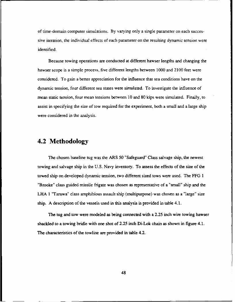
4.2 Methodology
The chosen baseline tug was the ARS 50 "Safeguard" Class salvage ship, the newest
towing and salvage ship in the U.S. Navy inventory. To assess the effects of the size of the
towed ship on developed dynamic tension, two different sized tows were used. The FFG 1
"Brooke" class guided missile frigate was chosen as representative of a "small" ship and the
LHA 1 "Tarawa" class amphibious assault ship (multipurpose) was chosen as a "large" size
ship. A description of the vessels used in this analysis is provided in table 4.1.
The tug and tow were modeled as being connected with a 2.25 inch wire towing hawser
shackled to a towing bridle with one shot of 2.25 inch Di-Lok chain as shown in figure 4.1.
The characteristics of the towline are provided in table 4.2.
48
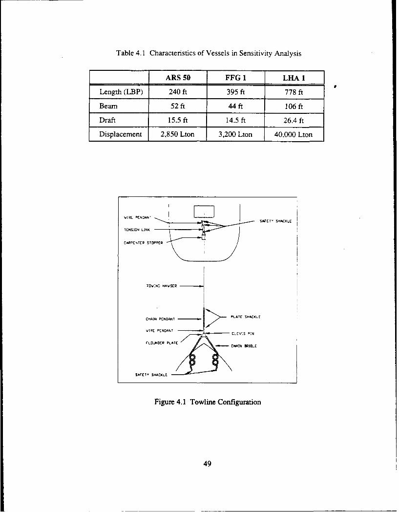
Table 4.1 Characteristics of Vessels in Sensitivity Analysis
ARS 50 FFG 1 LHA 1
Length (LBP) 240 ft 395 ft 778 ft
Beam 52 ft 44 ft 106 ft
Draft 15.5 ft 14.5 ft 26.4 ft
Displacement 2,850 Lton 3,200 Lton 40,000 Lton
WIRE PNDAN'SAFETY SHACKLE
TENSION LINK
CARPENTER STOPPER
TCVING HAWSER
CHAIN PENDANT ] PLATE SHACKLE
WIRE PENDAN
FLOUNDER PLATE CANBIL
SArETY SHACKLE
Figure 4.1 Towline Configuration
49

Table 4.2 Characteristics of Towline in Sensitivity Analysis
Wire Chain
Type 6x37 IWRC (EPS) Di-Lok
Length 1000 - 2100 ft 70 ft
Size 2.25 in 2.25 in
Elastic Modulus 12.6 x 10⁶ psi 30.0 x 10⁶ psi
Weight in water 8.31 lbs/ft 43.5 lbs/ft
Cross Sectional Area 2.35 in2 7.85 in2
Breaking Strength 444.6 kips 549 kips
The theory for dynamic towline extension and extremal statistics developed at MIT
was then applied to these ships. The ARS 50 was modeled towing at a speed of three knots
in head seas. Since values for added resistance have only been developed for stationary ves-
sels and since towing at high speeds is impractical, a speed of three knots was chosen as the
most realistic towing speed that also closely approximates zero Froude number. Heading
seas were chosen to be the most common encountered while towing at higher sea states,
because, as the sea state increases, the tug and tow will generally be forced to head into the
seas. The Pierson-Moskowitz sea spectrum was used to simulate wind speeds varying
between 15 and 30 knots. The use of unidirectional sea states was considered a valid approx-
imation since the resulting extreme extensions and tensions have been found to differ only
slightly from those of directional spectra (Milgram, 1988). Thus by using unidirectional
fully developed seas, wind speed may be used to specify different sea conditions.
Since surge is the primary motion influencing hawser elongation, it was the only ship
motion considered in the time-series simulations. Errors resulting from the neglect of the
influence of the other motions on the dynamic tension are considered unimportant for this
50

analysis. The two exciting forces were considered to be the Froude-Krylo" surge force and
added resistance. They account for both high and low frequency forces which cause fast and
slow surge motions on the two ships.
The initial step in the time-series evaluation was to model the surface wave surface ele-
vations (t) as a function of the input amplitude spectrum S(o) (Comstock, 1967):
N
(t) = " ,cos(c0t +e,) (4.1)
where:
= 2S(o,)Ao = wave elevation amplitude
N. Aw = number and interval of frequency subdivisions
S(o,) = input amplitude spectrum (Pierson-Moskowitz)
eS = random phase uniformly distributed between 0 and 27c
The first order, high frequency excitation force FFK(t) was similarly modeled:
NFFK(t) = X I FK(o))l , cos(°),t + s, + 4),) (4.2)
'-I
where:FK(w,) = Froude-Krylov surge exciting force
, = phase difference between Froude-Krylov surge force andsurface elevation at each frequency
The second order, low frequency excitation force F,"9'(t) was similarly modeled as the
added resistance of the ship.; in waves. The added resistance represents the increase in hull
resistance as compared to calm water conditions caused by the interaction of the waves with
the hull. The added resistance operator, R (w), which can be expressed as a function of wave
frequency, is proportional to the square of the wave amplitude, thus generating a low fre-
51

quency exciting force. The work of Kim and Yue (1989) was adopted to approximate this
second order, slowly-varying surge drift exciting force as a function of the wave elevation
and the added resistance in waves, R(co):
N N
Fx"'(t) = j XX ,RR(a)cos[(o, -oj)t +(,-) ] (4.4)
The surge motions resulting from these two exciting forces were coupled with the Numerical
Towline model (equation 1.6) to generate a time-series of dynamic tensions. To more realis-
tically identify the conditions in which significant dynamic tensions could be expected, the
different cases were compared based on the root mean square (RMS) value of dynamic
tensions. To better illustrate the relative magnitude differences between the mean and
dynamic tensions, all figures are presented in non-dimensionalized form with the RMS
dynamic tension divided by the mean tension.
4.3 Influence of Cable Length
As shown in figure 4.2, the RMS dynamic tension developed in a towing cable
decreases as length is increased. This can be explained by analysis of the geometry of the
cable. As the length of cable is increased, there is less restoring force present in the hawser.
This allows the ships to move more in response to wave excitation and hawser tension. The
cable is now said to have a "softer" spring constant as the additional sag in the catenary will
allow the hawser to absorb these larger elongations without a large increase in dynamic ten-
sion. Cross-flow drag, which has been found to increase the non-linear tension under certain
circumstances (section 1.1), also adds to the damping of the whole 12 DOF system.
52

0.9 - LLength /
0.8 - 1000 ftI
1200 ft0.7 - /-
.9 1500 ft
- 06 -- 1800 ft
... 210O0 ft
--
0.6 -S 0.5 -
0.2
' 0.4- ... ..
0
15 20 25 30
Wind Speed (knots)
Figure 4.2 Influence of Cable Length (LHA at 40 kips mean tension)
Although cable tension is affected by cross flow drag and other non-linearities, the
major influence on it is the nature of the static tension versus elongation curve (figure 1.1).
Since this curve does not account for any dynamic effects, it defines the lower bound on the
extreme tension. Cable stiffness is defined as the local slope on the static curve at a given
mean tension. Stiffer geometry configurations have greater slope which, for the same
amount of extension, result in larger tension increases. For very large static tensions, when
the cable elongation enters the purely elastic region (above the "knuckle"), the slope remains
constant and the static spring constant (K,,.,,) can be expressed as a function of cross sec-
tional area (A), modulus of elasticity (E) and length (L) as:
AEK,,.,, _ A (4.5)
53

Figure 4.3 presents the static curves for three different lengths of the ARS 50 hawser.
As hawser length increases, the static curve is displaced to the right and the range of the
"catenary" region is extended. Similarly, for the same value of static mean tension, the local
slope of the curve decreases with increased hawser length. This further illustrates the effect
that increasing length has on decreasing hawser stiffness.
200
8- 1000 ft 1500 ft 2100 ft
160 -
140
120
- 100-
0 -
40 -
20
00 20 40 60 80 100 120 140 160 10 200 220 240 260
Change in Span (ft)
Figure 4.3 Static Tension versus Elongation Curve for ARS 50
The local sea conditions, as related to wind speed, influence the magnitude of the
dynamic tension developed at different cable lengths. At lower wind speeds, the dynamic
cable tensions become increasingly more insensitive to changes in length. However as wind
speed increases, changes in length have significant impact on the dynamic tensions devel-
oped which can vary by as much as the magnitude of the mean tension. All lengths of cable
54
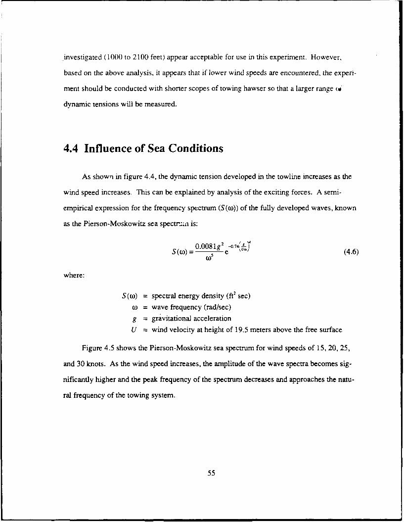
investigated (1000 to 2100 feet) appear acceptable for use in this experiment. However,
based on the above analysis, it appears that if lower wind speeds are encountered, the experi-
ment should be conducted with shorter scopes of towing hawser so that a larger range (i
dynamic tensions will be measured.
4.4 Influence of Sea Conditions
As shown in figure 4.4, the dynamic tension developed in the towline increases as the
wind speed increases. This can be explained by analysis of the exciting forces. A semi-
empirical expression for the frequency spectrum (S(o)) of the fully developed waves, known
as the Pierson-Moskowitz sea spectru.ni is:
S t ) -0 .0 0 8 lg 2 -0.7 , ) N4 .
_ W5o81 e0 1 (4.6)
where:
S (o) = spectral energy density (ft2 sec)
o = wave frequency (rad/sec)
g = gravitational acceleration
U = wind velocity at height of 19.5 meters above the free surface
Figure 4.5 shows the Pierson-Moskowitz sea spectrum for wind speeds of 15, 20, 25,
and 30 knots. As the wind speed increases, the amplitude of the wave spectra becomes sig-
nificantly higher and the peak frequency of the spectrum decreases and approaches the natu-
ral frequency of the towing system.
55
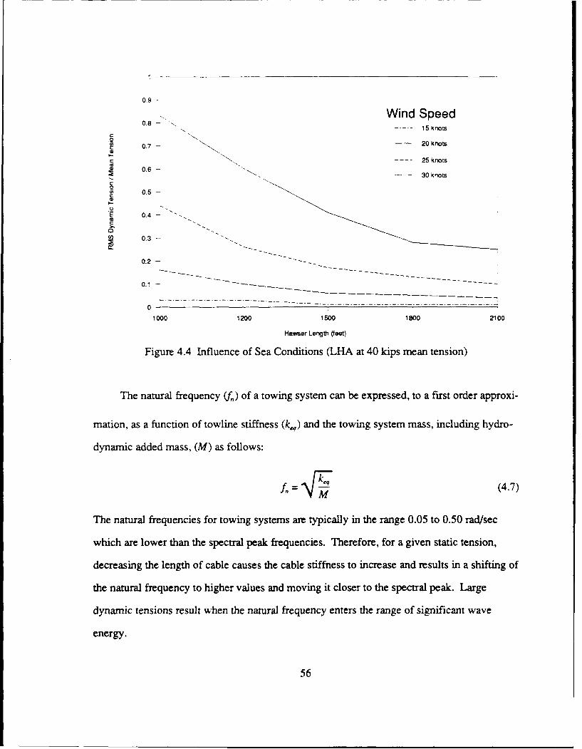
0.9 -
.8 Wind Speed0.8 - N.--- nt.\ ..... 15 knots
9 N. --- 20 knots
0.7 -
-,.. 25 knots
0.6- -30 knots
C
E. 0.
0.3-
0.2-
0
1000 1200 1500 1800 2100
Hawser Length (feet)
Figure 4.4 Influence of Sea Conditions (LHA at 40 kips mean tension)
The natural frequency (f,,) of a towing system can be expressed, to a first order approxi-
mation, as a function of towline stiffness (k,,) and the towing system mass, including hydro-
dynamic added mass, (M) as follows:
f, M (4.7)
The natural frequencies for towing systems are typically in the range 0.05 to 0.50 rad/sec
which are lower than the spectral peak frequencies. Therefore, for a given static tension,
decreasing the length of cable causes the cable stiffness to increase and results in a shifting of
the natural frequency to higher values and moving it closer to the spectral peak. Large
dynamic tensions result when the natural frequency enters the range of significant wave
energy.
56

45
40 -
Wind Speed35 -
30- -- 20 knots
I-- 25 knots
25- 30 knots
U) 20-
E.\
10- \
0 ---- - - - ......
0.100 0.200 0.300 0.400 0.500 0.600 0.700 0.800 0.900 1.000 1.100 1.200 1.300 1.400 1.500
Wave Frequency (rad/sec)
Figure 4.5 Pierson-Moskowitz Sea Spectrum
As related to sea conditions, the magnitude of the RMS dynamic tension is influenced
by the length of towing cable, especially at shorter lengths. This is because the decreased sag
in the catenary results in an increase in the cable stiffness which, in turn, increases the
dynamic tensions. As the length of the cable is increased, the influence of the wind dimi-
nishes rapidly as more cable sag is present to dampen and absorb the effects of the end point
extension.
The dynamic tension at 15 knots wind speed differed from the mean tension by, at
most, four percent for all conditions investigated. This is considered to be too small for dis-
crimination from "noise" in the mean tension levels during an experiment. Therefore, the
lower threshold for the actual wind speed (ship's speed plus relative wind speed) for the
57

experiment should be greater than 15 knots. It is highly desirable to have wind speeds higher
than 20 knots to develop measurable differences between the dynamic and mean static ten-
sions.
4.5 Influence of Mean Tension
As shown in figure 4.6, increasing the mean cable tension results in an increase in the
magnitude of the dynamic tension. Changes in mean tension are generally developed by a
change in the span between two ships. As the hawser straightens out, the sag of the catenary
is reduced. The effect of this is to reduce the cable's ability to absorb further extensions
without a significant increase in the dynamic tension. This can also be seen by the hawser's
static tension versus elongation curve (figure 4.3). Increasing the mean tension results in a
larger local slope on the curve and so larger dynamic tensions result from the same amount of
elongation. To achieve distinct and measurable dynamic tensions during the experiment,
shorter scopes of hawser should be used when lower values of mean tension are present.
4.6 Influence of Size of Tow
Up to now, only discrete mean tensions, chosen "a priori," have been investigated.
However, this procedure cannot be used directly to investigate the influence of the size of
tow on the developed dynamic tensions. This is because each vessel will have a different
mean tension value depending upon its unique hull form and characteristics. Therefore, an
estimated value of the mean static for each ship must be computed before' .omparison
between different sized ships can be accomplished.
58
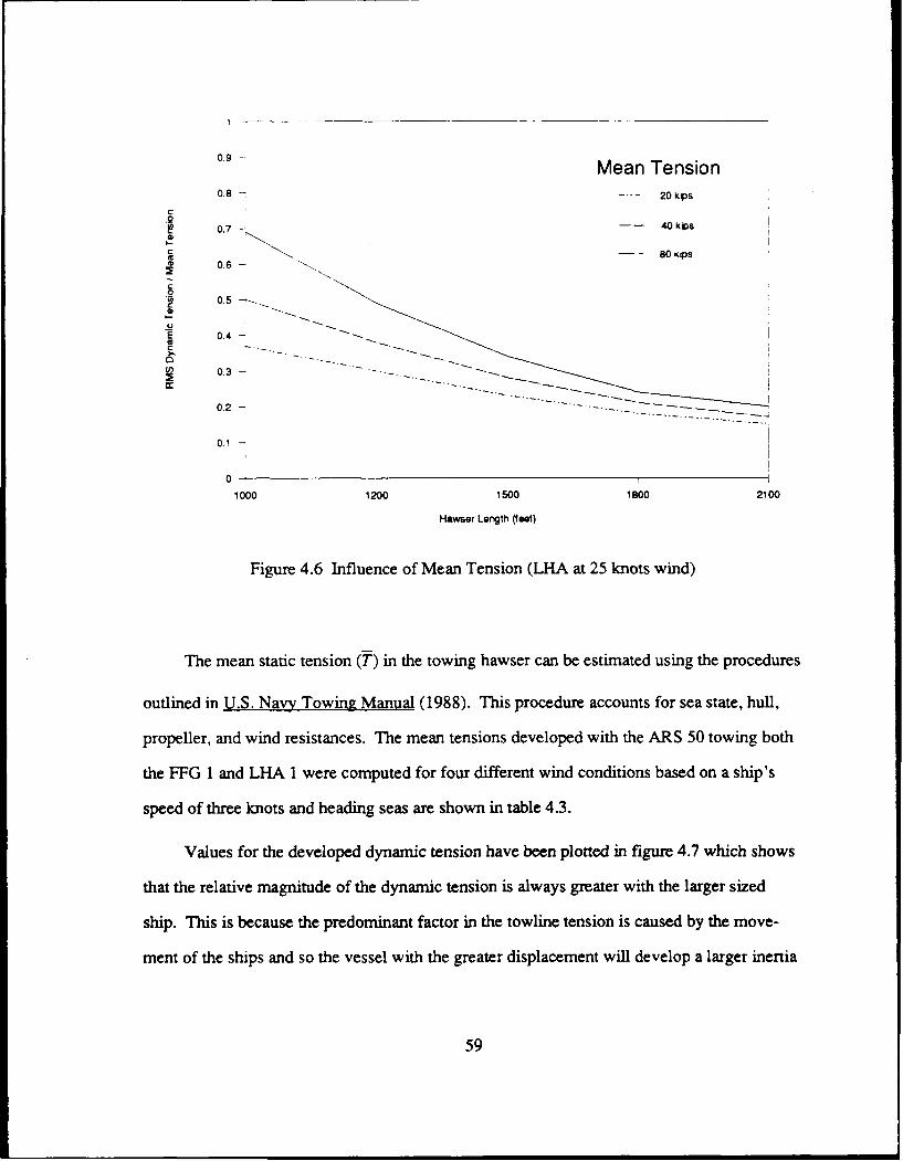
0.9 Mean Tension
0.8 -- 20 kips
0.7 - 40 kPs
0.-C 80 ips0.-
C.0 W 0.5
C
E0.
0.3 ---
0.2-
0.1-
0
1000 1200 1500 1Boo 2100
Hawser Length (feet)
Figure 4.6 Influence of Mean Tension (LHA at 25 knots wind)
The mean static tension (T) in the towing hawser can be estimated using the procedures
outlined in U.S. Navy Towing Manual (1988). This procedure accounts for sea state, hull,
propeller, and wind resistances. The mean tensions developed with the ARS 50 towing both
the FFG 1 and LHA 1 were computed for four different wind conditions based on a ship's
speed of three knots and heading seas are shown in table 4.3.
Values for the developed dynamic tension have been plotted in figure 4.7 which shows
that the relative magnitude of the dynamic tension is always greater with the larger sized
ship. This is because the predominant factor in the towline tension is caused by the move-
ment of the ships and so the vessel with the greater displacement will develop a larger inertia
59

Table 4.3 Expected Mean Tensions at 3 knots, heading seas
FFG 1 LHA 1
wind speed T
15 knots 12 kips 31 kips
20 knots 14 kips 40 kips
25 knots 17 kips 55 kips
30 knots 23 kips 80 kips
while towing. The distinction in size diminishes at lower wind speeds and longer lengths of
towing hawser because the hawser is able to absorb more extension with little change in
dynamic tension. The phase difference between the surge motions of the tow and tow will
then be the prime factor in determining the magnitude of the developed dynamic tensions.
Figure 4.7 shows that there is a trade off between wind speed and the size of tow. At
higher wind speeds (25 knots) the importance of vessel size diminishes as measurable
dynamic tensions can be obtained from either size vessel. However, at lower wind speeds
the length of the towing hawser becomes more significant. At 15 knots of wind, the magni-
tude of the dynamic tension developed by either size vessel is so small that it is doubtful that
meaningful measurements could be recorded. Based on these observations, the experiment
should be conducted with a larger sized vessel because the developed RMS dynamic tension
was always greater than the smaller vessel. To achieve measurable dynamic tensions with
smaller sized tows, it is recommended to tow at shorter hawser lengths.
60

0.9 -
wind
0.8 Small Large15 knots
.20.7 20 knots
25 knots
* 0.6
00.5
C
0.
........... .. ...
. . ... ... .. ....
... ............... - .......- --n. -- - . -
1000 1200 1500 1800 2100
Hawser Length (feet)
Figure 4.7 Influence of Size of Tow (25 knots wind)
4.7 Summary
From the above analyses, it is obvious that all four factors investigated (sea conditions,
hawser length, mean tension, and size of tow) are interrelated and affect the dynamic tensions
developed while towing to different extents. Since the purpose of this validation experiment
is to compare measured tensions to analytical predictions, it is necessary that a wide range in
dynamic tensions be developed in the hawser. This will allow greater discrimination
between the different cases and help to ensure that meaningful results are obtained.
61

The most important factor influencing the magnitude of the dynamic tension is the
mean tension as it defines the location on the static tension versus elongation curve. The
local sea conditions and hawser length also contribute significantly to the development of
dynamic tensions. The local sea conditions appear to have a greater influence the develop-
ment of dynamic tensions than the effect of changing hawser length. This is expected
because tension is a function of cable elongation (equation 1.6) and sea conditions cause the
ships to move which results in cable elongations. Based on these analyses, the experiment
must be conducted in a region with local wind speeds of 18 knots or more in order to develop
needed measurable differences in dynamic tensions.
In addition to sea conditions, dynamic tensions appear to be highly sensitive to hawser
length. Increasing the length of the towing hawser significantly reduces the dynamic tension
as the cable becomes "softer." In all cases investigated, shorter hawser lengths provided a
wider range of dynamic tensions. Therefore, shorter scopes of towing hawser should be used
in the experiment when lower values of mean tension are anticipated and when smaller sized
tows are used.
62

Chapter Five
Equipment Selection
5.1 Measurement Specifications
The initial step in the selection of instrumentation was to define a set of measurement
specifications. The goal was to specify the required measurement tolerances for each instru-
ment that would provide sufficient resolution for proper analysis. This was based both on an
analysis of previous test plans, Milgram (1986), and the analytical model predictions
obtained during the sensitivity analysis (chapter 4). A summary of the measurement specifi-
cations for this experiment is provided in Table 5.1. In addition to specifying a frequency
and anticipated range of values for each measured parameter, a required precision has been
expressed in terms of an absolute error. All dynamic measurements include a relative error
which is based on the overall system error, riot just the individual sensor itself.
5.2 Provision of Instrumentation
To accomplish this experiment, complex and highly specialized instrumentation is
needed. A primary consideration in the selection of instrumentation was the desire to allo-
63

cate responsibility for all data signals to a single organization. This would not only minimize
confusion and misunderstanding of individual responsibilities but also, hopefully, reduce
field problems by allowing all instrumentation to be assembled and tested in a single labora-
tory prior to installation. Other significant factors used in the selection of equipment were
compactness, reliability, accuracy, self sufficiency, and having sufficient resolution to
provide statistically significant data even when sea conditions are relatively calm. Every
attempt to minimize interference with or dependence upon installed shipboard systems was
made. Several possible methods of obtaining the required instrumentation were investigated;
provision by a U.S. Navy laboratory, assembling it using resources available at MIT, or sub-
contracting to a commercial company.
Several Navy laboratories are experienced in measuring ship motions arnd environmen-
tal conditions. Both the David Taylor Research Center (DTRC) and the Naval Civil Engi-
neering Laboratory (NCEL) in Port Hueneme, California offered assistance. However, since
they both could only provide a limited amount of the required instrumentation, the use of a
U.S. Navy laboratory was found to be infeasible for this experiment. The cost and lead time
of acquiring the highly specialized equipment made it uneconomically feasible to attempt
outfitting directly at MIT. Therefore, the most economical alternative was found to subcon-
tract out to a commercial company. Table 5.2 provides a listing of all instrumentation
selected for the experiment.
5.3 The Tug and Tow
The selection of naval ships for use in the experiment was based primarily on availabil-
ity of resources rather than meeting any specific design specifications. However, a conscious
64

Table 5.1 Measurement Specifications
Parameter Frequency Range Absolute Relative(Hz) Error Error
WindSpeed 0-0.2 0 - 50 knots 1.0 knot -
Direction 0 - 0.2 0 - 360 deg. 1.0 deg. -
Speed 0-0.2 0 - 15 knots 0.1 knot -
Heading 0 - 0.2 0 - 360 deg 1.0 deg. -
Separation 0 - 0.2 300 - 2000 ft 4.0 ft -
Hawser anglehorizontal 0 - 0.2 ± 45 deg. 1.0 deg -
vertical 0- 0.2 0 - 80 deg. 1.0 deg
Tension 0.015 - 2.0 2 - 100 kips 200 lbs
Surge 0.015 - 0.3 ± 25 ft 0.1 ft 2%
Sway 0.015 -0.3 ± 25 ft 0.1 ft 2%
Heave 0.015 - 0.3 ± 25 ft 0.1 ft 2%
Roll 0.015 - 0.3 ±25 deg 0.5 deg. 3%
Pitch 0.015-0.3 10 deg 0.2 deg. 3%
Yaw 0.015 - 0.3 ± 10 deg 0.2 deg. 3%
Wave Height 0.03 - 0.3 ± 25 ft 0.1 ft 2%
effort was made to find a "larger" sized vessel to help in obtaining a wider range of dynamic
tensions as shown in chapter 4. The two naval vessels selected to participate in this experi-
ment are the USS SALVOR (ARS 52) and the ex-USS HECTOR (AR 7). The characteristics
of these ships are shown in Table 5.3.
The USS SALVOR (ARS 52) is a "Safeguard" Class Salvage ship. Commissioned on
14 June 1986, the SALVOR is a member of the newest salvage ship in the U.S. Navy inven-
tory. She is powered by four Caterpillar D-399 diesel engines which produce a total of 4200
SHP. The SALVOR has an Almond A. Johnson Series 322 automatic towing machine which
65

Table 5.2 Summary of Instrumentation
Item Manufacturer Model Number
Tension StrainSert Tension Link STL-80 (SS)StrainSert Clevis Pin SPA 180-1.5 SGK
Wind Skyvane Wind Sensor 2101
Wave Height TSK wave height meter ---
Speed Northstar LORAN C 5000
Heading Cetrek Electronic Compass 930-550
Range Dr. Rigel Laser Range Finder LR90-80
Signal conditioners VISHAY amplifier 2310
Motions Humphrey vertical gyro VG 34-0301-1Glennite accelerometers LA 820201
holds 3000 feet of 2.25 inch wire towing hawser in addition to a series 400 traction winch for
14 inch fiber rope hawsers. The SALVOR is capable of producing 138,000 pounds of bol-
lard pull thrust.
The ex-USS HECTOR (AR 7) is a "Vulcan" Class Repair ship commissioned on 7 Feb-
ruary 1944. She was recently decommissioned from active duty in the U.S. Navy and is cur-
rently moored at the Naval Station Pearl Harbor, Hawaii awaiting transfer to the Pakistani
Navy. The HECTOR is currently in the custody of the Inactive Ship Maintenance Facility,
Pearl Harbor, Hawaii. Permission from the office of the Chief of Naval Operations (CNO)
has been obtained to use the vessel in this towing experiment prior to the transfer of owner-
ship.
66

Table 5.3 Gross Characteristics of Test Platforms
TUG TOW
Ship ARS 52 AR 7
Length (ft) 255 520
Beam (ft) 52 73
Draft (ft) 15.5 15.5
Displacement (Ltons) 2,850 10,130
67

Chapter Six
Analytical Predictions
6.1 Background
Since towing conditions must be set so the probability of towline failure is very small,
the U.S. Navy Towing Manual (1988) estimates extrer . tensions based on a probability of
0.1% of being exceeded in one day of towing. Since those extreme tensions occur, on the
average, only once in 1000 days of towing, they cannot be directly measured in a practical
experiment. Instead, the theory can be used to determine the most probable extreme tension
to be encountered during a discrete time interval, such as one hour, and can provide a com-
plete probability distribution function for the extreme tension during that time interval.
Agreement between measurement and theory would provide high confidence for application
of the theory to the more rare extremes of interest in actual towing operations.
Although fimal analysis and comparison of analytical tension predictions to actual mea-
surements can only be done upon completion of the experiment, analytical predictions must
be available prior to the experiment. This will provide a means of on-scene evaluation of the
data as it is being recorded which will help to identify errors in the measurement procedures.
68

Additionally, these predictions can be used to preselect conditions for conducting the experi-
ment such that a higher range of dynamic tensions can be anticipated. During the post-
voyage data analysis, the exact conditions that were measured can be individually input into
the different analytical models and the results compared with actual measurements. In this
manner, each phase of the model can be individually verified or modified as necessary to
achieve good correlation between the analytical predictions and actual measurements.
6.2 Methodology
To obtain a set of predictions for the experiment, the analytical method outlined in sec-
tion 1.3 was used. Ship motion responses to different sea conditions were computed using
seakeeping theory based on the proposed towline configuration (table 6.1). The influence of
towline tension on these motions was then accounted for using the method of equivalent line-
arization. The resulting ship motions were then coupled with the Numerical Towline Model
to evaluate dynamic tensions. To account for the unknowns during actual measurement
during the experiment, three speeds, four relative wave angles, four different mean tensions
and five different hawser lengths were modeled. Since it is highly unlikely that an extreme
tension will be encountered during the short duration of testing, the analytical predictions are
based on the RMS values of tension which were computed from the zeroeth moment of the
tension spectrum.
The resulting predictions comprise a large set of data which is presented in Appendix
B. To simplify the presentation, the data is displayed in a series of 16 different curves (fig-
ures B. I through B. 16). An estimate for the RMS value of tension for a specific condition
can be thus be obtained by interpolating between the different graphs.
69
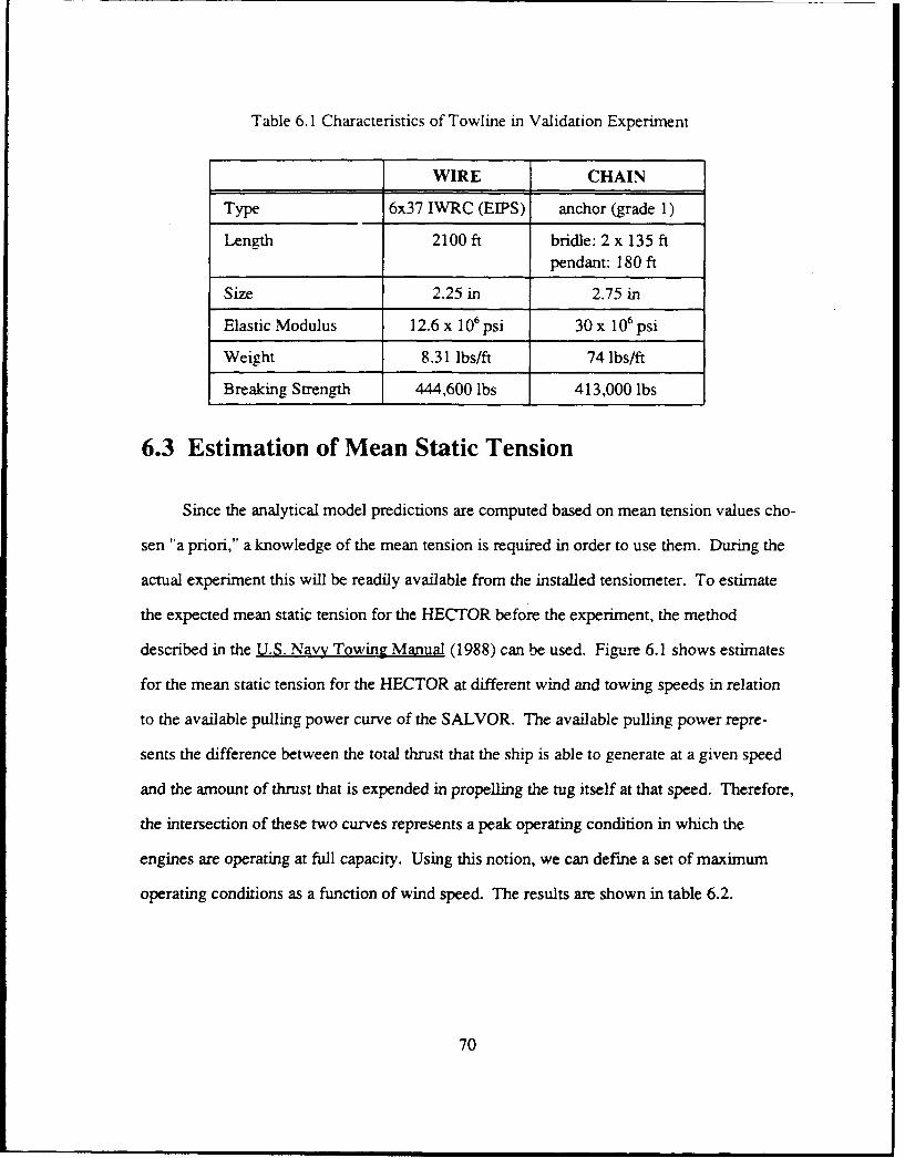
Table 6.1 Characteristics of Towline in Validation Experiment
WIRE CHAIN
Type 6x37 IWRC (EIPS) anchor (grade 1)
Length 2100 ft bridle: 2 x 135 ftpendant: 180 ft
Size 2.25 in 2.75 in
Elastic Modulus 12.6 x 10⁶ psi 30 x 106 psi
Weight 8.31 lbs/ft 74 lbs/ft
Breaking Strength 444,600 lbs 413,000 lbs
6.3 Estimation of Mean Static Tension
Since the analytical model predictions are computed based on mean tension values cho-
sen "a priori," a knowledge of the mean tension is required in order to use them. During the
actual experiment this will be readily available from the installed tensiometer. To estimate
the expected mean static tension for the HECTOR before the experiment, the method
described in the U.S. Navy Towing Manual (1988) can be used. Figure 6.1 shows estimates
for the mean static tension for the HECTOR at different wind and towing speeds in relation
to the available pulling power curve of the SALVOR. The available pulling power repre-
sents the difference between the total thrust that the ship is able to generate at a given speed
and the amount of thrust that is expended in propelling the tug itself at that speed. Therefore,
the intersection of these two curves represents a peak operating condition in which the
engines are operating at full capacity. Using this notion, we can define a set of maximum
operating conditions as a function of wind speed. The results are shown in table 6.2.
70

150
140 - Wind Speed
130 - 10 knots
120 -/ 15 knots/
110 - ...... 20 knots100/ 25 knots
90 -30 knots
so -70
60
50 - /-
40 -
3010- 7 -!----A aia l e so
0 -
0 2 4 6 8 10 12 14 16
Towing Speed (knots)
Figure 6.1 Estimated Mean Tension and Available Pulling Powerfor the SALVOR towing the HECTOR
Table 6.2 Maximum Operating Conditions for the experiment (1000 ft hawser)
Wind Speed Maximum Towing Mean Static Tension(knots) Speed (knots) (kips)
15 9.0 78
20 8.5 82
25 7.8 90
30 6.6 100
71

6.4 Analytical Predictions
The analytical predictions of RMS towline tension appear to be consistent with rela-
tionships identified in the sensitivity analysis (chapter 4); shorter hawser lengths show
greater dynamic tension extremes, especially at higher values of mean tension and that wind
speeds greater than 15 knots are required in order to have measurable dynamic tensions
developed. This can be seen in figure 6.2, which contains plotted data from the tables B.A
through B. 12.
150 +.
140 Mean Tension130- 9 knots 10 kips
13O
10-
10
40kips
30 -
10 -------------------------------
60-
30 -
1000 1200 1400 1600 1800 2000
Haww Lngwt (feot)
Figure 6.2 ARS 52 towing AR 7 at relative wave angle 000, wind speed 20 knots
72

Comparison of dynamic tensions developed while towing at different wave angles. as
shown in figures 6.2 and 6.3, reveals that the magnitude of the developed dynamic tension is
highly dependent upon the relative wave angle, especially at higher values of mean ten~ion.
Heretofore, only heading seas (relative wave angle of 180 degrees) were investigated because
heading seas are the most common encountered while towing at higher sea states, since, as
the sea state increases, the tug and the tow will generally be forced to head into the seas. For
a given mean tension, the largest dynamic tensions are developed in following seas (relative
wave angle equal to zero degrees) and the magnitude of the dynamic tensions decreases dra-
matically as the relative wave angle increases. This is because in following seas, the fre-
quency spectrum of the seas tunes with the natural frequency of the towing system which
results in greater ship motions and therefore larger dynamic tensions.
150
140- Mean Tension130 10 .... Okips
120 9 knots 20kips
110 - 6 knots
100 - 3 nt; 80 kips
S 90
0
70-
2 r'60 -
50-
40
1000 1200 1400 1600 1800 2000
Hawse Lewgth (feet)
Figure 6.3 ARS 52 towing AR 7 at relative wave angle 180, wind speed 20 knots
73

In the sensitivity analysis we found that wind speeds greater than 15 knots were needed
when towing at three knots in order to have measurable dynamic tensions developed. This
corresponds to a significant wave height of 4 feet. Based on the historical mean wind speeds
off Oahu, figure 2.1 the average mean wind speed is approximately 13 knots. However,
when more specific statistical wave height information is investigated (table 6.3), we see that
the there is a 90% probability that the wave height will be 6.6 feet or greater. This corre-
sponds to a sea state of five that would typically have a wind speed of 19 knots. The reason
for the wave heights to be larger than typical predictions can be attributed to the fact that
Hawaii is an island and there are very long fetch lengths. Since the effect of sea conditions
on the motions of the ship is largely a function of wave height, and not wind speed, this fur-
ther emphasizes the conclusion in chapter two that Hawaii is the optimum location to conduct
the experiment.
Table 6.3 Statistical Wave Height Data near Oahu, Hawaii (April 1986)(Mariners Weather Log, Vol 30)
buoy 3.3-4.9 ft 6.6-8.2 ft 9.8-11.5 ft 13.1-14.8 ft Maximum Mean
51002 9.7% 41.7% 46.3% 2.2% 13.1 ft 8.5 ft
51003 9.3 % 64.0% 20.4 % 6.1% 18.0 ft 8.2 ft
51004 3.1 % 50.4 % 40.6 % 5.6 % 14.8 ft 8.9 ft
51005 10.3% 51.4% 30.3% 7.8% 18.0 ft 8.5 ft
Figures 6.2 and 6.3 show that towing speed has very little influence on the dynamic
tensions below 20 kips mean tension. This indicates that the primary factor developing the
tension is due to seakeeping response of the ships rather than due to additional engine thrust.
74

During the experiment, when the actual wind conditions and static mean tension will be
known, these predictions can be very useful in selecting the hawser scope, speed. and course
to tow on during each data collection period to have a greater certainty of experiencing larger
and more measurable dynamic tensions.
75
Chapter Seven
Conclusions
7.1 Summary
This study has been a practical extension of previous work done at MIT on the dyna-
mics of tension in towing hawsers. A sensitivity analysis has been conducted to investigate
the relative importance of various parameters (hawser length, wind speed, mean tension, and
size of tow) on the magnitude of the resulting dynamic tensions. Although all lengths are
acceptable for measurement purposes, shorter hawser lengths provide larger range in
dynamic tensions. A lower bound on wind speed has been established at 18 knots when tow-
ing at three knots. Based on a parametric study and analysis of coastal weather patterns,
Hawaii has been selected as the best test location. Equipment selection was based on a set of
developed measurement specifications.
As a result of this work, a validation experiment has been planned, organized, and
scheduled. The Navy has designated two ships, the USS SALVOR (ARS 52) and the ex-
USS HECTOR (AR 7), to be test platforms for the validation experiment. The experiment is
scheduled for early May off the coast of Oahu, Hawaii. All equipment needed for this
76

experiment has been assembled. tested, and is ready for shipment. A series of analytical pre-
dictions, based on the RMS values of tension, have been developed (Appendix B) for on-
scene data analysis and to assist in the selection of the best course and speed combination to
obtain measurable dynamic tensions during the experiment. Appendix C provides the test
plan that has been developed and issued to all involved personnel specifying the procedures
and support requirements for the experiment. Unfortunately, the late date of this experiment
precludes the inclusion of any post-voyage analysis with this study. However, upon comple-
tion of the experiment, a full report will be issued describing the results.
7.2 Further Studies
This work represents the first step in confirming the applicability of the MIT analytical
model used to predict dynamic towline tension extremes. Post-voyage analysis of data col-
lected during the towing experiment will hopefully verify the approach taken or indicate
weaknesses which can then be modified using the measured results as a benchmark to
achieve better correlation.
The experiment has been planned to measure a wide variety of parameters to generate a
wealth of raw data for further analysis. Although the main purpose is to conduct seakeeping
tests to confirm the influence of ship motions, especially surge, on cable extension and the
resulting dynamic tension, four other tests are planned in conjunction with this; towing
machine dynamic response test, fiber rope test, elastic wave test, and a transient response
test.
The analytical models used to predict extreme tensions are based on ship motions as
influenced by linear towline forces using the method of equivalent linearization. However, if
77
the actual non-linear forces and moments on the ship due to the towline could be predicted,
the accuracy of the model would improve. Comparison of measured values to the linear
approximations could provide an insight into predicting these non-linear forces. Addition-
ally, the influence of the second order, slowly-varying component of dynamic tension (T.,)
has been neglected in all analyses to date. It is hoped that by measuring the time history
change in hawser horizontal angle, a relationship can be found to account for this in future
work.
This study has only investigated wire rope towlines. Since fiber ropes are lighter and
softer, their tension verses extension behavior should be much less non-linear than the wire
and so easier to predict. An analytical model has been developed to predict the tension
extremes in fiber towing hawsers (Milgram, 1988). All measurement procedures and instru-
ments used for the wire rope analysis are suitable for a similar analysis of fiber cables. The
last day of the experiment is now planned to include measurement while towing with a fiber
towing hawser. Hopefully, data collected during this experiment can also validate that ana-
lytical model.
78

References
Anagnostou, G. (1987). Extreme tension in a ship's towline. Master's thesis, Massachusetts
Institute of Technology, Department of Ocean Engineering, Cambridge, MA.
Bhattacharyya, R. (1978). Dynamics of marine vechiles. New York: Wiley.
Campman, C. R., & Debord, F. W. (1985). Tow monitoring system design for the real
world (OTC 5045). Paper presented at the 17th Annual Offshore Technology Confer-
ence, Houston.
Comstock, J. P. (Ed.). (1967). Principles of naval architecture (rev. ed.). New York: The
Society of Naval Architects and Marine Engineers.
DeBord, F. Jr., Purl, J., Mlady, J., Wisch, D., & Zahn, P. (1987). Measurement of full-scale
barge motions and comparision with model test and mathematical predictions.
SNAME Transactions, 95, 319-335.
Durgin, F. H. (1975). Use of anemometers in on-site studies of buildings and structures ani
in particular the Bendix Frieze anemometers. Unpublished manuscript, Massachusetts
Institute of Technology, Wright Brothers Wind Tunnel, Cambridge, MA.
Frimm, F. D. C. (1987). Non-linear extreme tension statistics of towing hawsers. Doctoral
dissertation, Massachusetts Institute of Technology, Department of Ocean Engineering,
Cambridge, MA.
Frimm, F. D. C. and Milgram, J H. (1986). Analysis of full-scale towing experiments.
Unpublished document.
Kim, M. H. & Yue, D.K.P. (1989). Slowly-varying wave drift forces in short-crested irregu-
lar waves. Applied Ocean Research, JI(1), 2-18.
Loukakis, T. (1970). Computer-aided prediction of seakeeping performance in ship design
(Technical Report). Cambridge, MA: Massachusetts Institute of Technology.
Milgram, J., Triantafyllou, M., Frimm, F., Anagnostou, G. (1988). Seakeeping and extreme
tensions in offshore towing. Paper presented at the Annual Meeting of the Society of
Naval Architects and Marine Engineers, New York.
79

Milgram, J. H. (1986). Plans and specifications for towing test measurements. Unpublished
document.
Naval Sea Systems Command. (1988). U.S. Navy Towing Manual (rev. 1) (SL740-AA-
MAN-010). Washington, DC.
Salvesen, N., Tuck, E. 0., & Faltinsen, 0. (1970). Ship motions and sea loads. SNAME
Transactions, 78.
Sellars, F. H. (1967). The dynamic calibration of shipborne wave gages (Report No. 67-11).
Cambridge, MA: Massachusetts Institute of Technology.
Triantafyllou, M. S. (1987). Nonlinear dynamics of marine cables and hawsers (Technical
Report). Cambridge, MA: Massachusetts Institute of Technology.
80
Appendix A
Salvage Ships of the U.S. Navy
81

The following is a list of Salvage Ships on active duty in the U.S. Navy which could be used
for the towing experiment.
POWHATAN Class Fleet Tugs
USNS POWHATAN (T-ATF 166)USNS NARRANGANSETT (T-ATF 167)USNS CATAWBA (T-ATF 168)USNS NAVAJO (T-ATF 169)USNS MOHAWK (T-ATF 170)USNS SIOUX (T-ATF 171)USNS APACHE (T-ATF 172)
SAFEGUARD Class Salvage Ships
USS SAFEGUARD (ARS 50)USS GRASP (ARS 51)USS SALVOR (ARS 52)USS GRAPPLE (ARS 53)
DIVER/BOLSTER Class Salvage Ships
USS PRESERVER (ARS 8)USS BOLSTER (ARS 38)
USS CONSERVER (ARS 39)USS HOIST (ARS 40)USS OPPORTUNE (ARS 41)USS RECLAIMER (ARS 42)USS RECOVERY (ARS 43)
EDENTON Class Salvage and Rescue Ships
USS EDENTON (ATS 1)USS BEAUFORT (ATS 2)USS BRUNSWICK (ATS 3)
82

ABNAKI Class Fleet Tugs
USS PAIUTE (ATF 159)USS PAPAGO (ATF 160)
PIGEON Class Submarine Rescue Ships
USS PIGEON (ASR 21)USS ORTOLAN (ASR 22)
CHANTICEER Class Submarine Rescue Ships
USS FLORIKAN (ASR 9)USS KITTIWAKE (ASR 13)
USS PETREL (ASR 14)
USS SUNBIRD (ASR 15)
83

Appendix B
Analytical Predictions
84

Table B.1 RMS Towline Tension (kips) for ARS 52 towing AR 7at 3 knots with 10 kips mean tension
Wave Wind 1000 ft 1200 ft 1500 ft 1800 ft 2100 ftAngle Speed
000 15 10.1 10.1 10.1 10.1 10.0
000 20 10.3 10.2 10.2 10.1 10.1
000 25 10.6 10.5 10.4 10.3 10.3
000 30 11.0 10.8 10.7 10.5 10.4
060 15 10.2 10.2 10.2 10.1 10.1
060 20 10.5 10.5 10.5 10.3 10.3
060 25 10.8 10.7 10.7 10.5 10.4
060 30 11.1 11.0 11.0 10.6 10.5
120 15 10.3 10.2 10.3 10.1 10.0
120 20 10.7 10.7 10.7 10.4 10.3
120 25 11.2 11.1 11.0 10.7 10.7
120 30 11.4 11.4 11.3 10.9 10.9
180 15 10.1 10.1 10.1 10.1 10.1
180 20 10.4 10.3 10.3 10.2 10.2
180 25 10.8 10.6 10.6 10.4 10.4
180 30 11.2 11.0 11.0 10.7 10.6
85
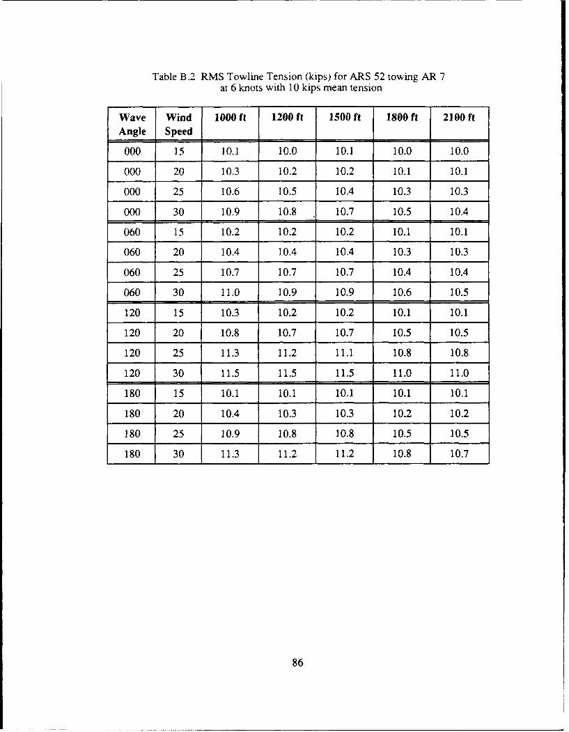
Table B.2 RMS Towline Tension (kips) for ARS 52 towing AR 7at 6 knots with 10 kips mean tension
Wave Wind 1000 ft 1200 ft 1500 ft 1800 ft 2100 ftAngle Speed
000 15 10.1 10.0 10.1 10.0 10.0
000 20 10.3 10.2 10.2 10.1 10.1
000 25 10.6 10.5 10.4 10.3 10.3
000 30 10.9 10.8 10.7 10.5 10.4
060 15 10.2 10.2 10.2 10.1 10.1
060 20 10.4 10.4 10.4 10.3 10.3
060 25 10.7 10.7 10.7 10.4 10.4
060 30 11.0 10.9 10.9 10.6 10.5
120 15 10.3 10.2 10.2 10.1 10.1
120 20 10.8 10.7 10.7 10.5 10.5
120 25 11.3 11.2 11.1 10.8 10.8
120 30 11.5 11.5 11.5 11.0 11.0
180 15 10.1 10.1 10.1 10.1 10.1
180 20 10.4 10.3 10.3 10.2 10.2
180 25 10.9 10.8 10.8 10.5 10.5
180 30 11.3 11.2 11.2 10.8 10.7
86

Table B.3 RMS Towline Tension (kips) for ARS 52 towing AR 7at 9 knots with 10 kips mean tension
Wave Wind 1000 ft 1200 ft 1500 ft 1800 ft 2100 ftAngle Speed
000 15 10.1 10.1 10.1 10.0 10.0
000 20 10.4 10.3 10.2 10.1 10.1
000 25 10.8 10.6 10.5 10.3 10.3
000 30 11.0 10.9 10.8 10.5 10.4
060 15 10.2 10.1 10.2 10.1 10.1
060 20 10.4 10.4 10.4 10.3 10.3
060 25 10.7 10.6 10.6 10.4 10.4
060 30 10.9 10.8 10.8 10.6 10.5
120 15 10.2 10.2 10.2 10.1 10.1
120 20 10.8 10.8 10.7 10.5 10.4
120 25 11.4 11.3 11.2 10.9 10.8
120 30 11.7 11.7 11.6 11.2 11.1
180 15 10.1 10.1 10.1 10.1 10.1
180 20 10.4 10.4 10.4 10.3 10.3
180 25 11.0 10.9 10.9 10.6 10.5
180 30 11.5 11.4 11.4 11.0 11.0
87

Table B.4 RMS Towline Tension (kips) for ARS 52 towing AR 7at 3 knots with 20 kips mean tension
Wave Wind 1000 ft 1200 ft 1500 ft 1800 ft 2100 ftAngle Speed
000 15 20.3 20.2 20.2 20.1 20.1
000 20 21.7 20.9 20.6 20.4 20.4
000 25 24.1 22.2 21.3 21.0 20.9
000 30 25.4 23.3 22.2 21.8 21.5
060 15 20.7 20.4 20.4 20.4 20.3
060 20 21.8 21.3 21.2 21.1 20.6
060 25 23.2 22.1 21.4 21.3 21.1
060 30 24.7 23.1 22.0 22.0 21.6
120 15 20.7 20.6 20.6 20.5 20.3
120 20 22.3 21.7 21.6 21.4 21.0
120 25 23.9 22.7 22.6 22.2 21.7
120 30 25.1 23.5 23.0 22.7 22.2
180 15 20.4 20.2 20.2 20.2 20.2
180 20 21.5 20.9 20.6 20.6 20.6
180 25 23.3 22.0 21.4 21.3 21.2
180 30 24.9 23.3 22.3 22.0 21.9
88

Table B.5 RMS Towline Tension (kips) for ARS 52 towing AR 7at 6 knots with 20 kips mean tension
Wave Wind 1000 ft 1200 ft 1500 ft 1800 ft 2100 ftAngle So ;d
000 15 20.5 20.3 20.2 20.1 20.1
000 20 22.3 21.2 20.7 20.5 20.4
000 25 24.6 22.7 21.5 21.2 21.0
000 30 24.0 23.5 22.6 22.0 21.7
060 15 20.7 20.4 20.4 20.4 20.3
060 20 21.9 21.2 21.1 21.0 20.6
060 25 23.3 22.0 21.8 21.5 21.0
060 30 24.8 23.1 22.5 21.9 21.5
120 15 20.7 20.6 20.5 20.5 20.3
120 20 22.4 21.9 21.7 21.5 21.1
120 25 24.1 23.0 22.6 22.4 21.9
120 30 25.3 23.7 23.3 23.0 22.5
180 15 20.3 20.2 20.2 20.2 20.1
180 20 21.4 20.9 20.7 20.7 20.6
180 25 23.4 22.1 21.6 21.5 21./
180 30 24.9 23.5 22.6 22.3 22.2
89
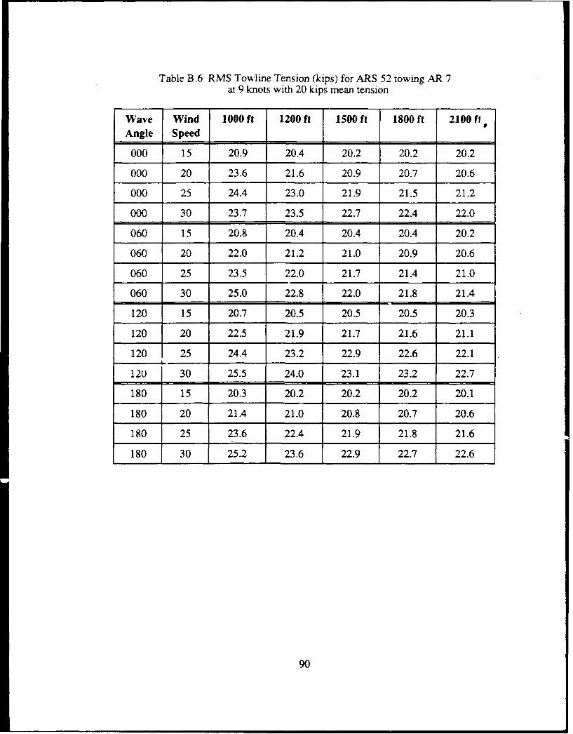
Table B.6 RMS Towline Tension (kips) for ARS 52 towing AR 7at 9 knots with 20 kips mean tension
Wave Wind 1000 ft 1200 ft 1500 ft 1800 ft 2100 ftAngle Speed
000 15 20.9 20.4 20.2 20.2 20.2
000 20 23.6 21.6 20.9 20.7 20.6
000 25 24.4 23.0 21.9 21.5 21.2
000 30 23.7 23.5 22.7 22.4 22.0
060 15 20.8 20.4 20.4 20.4 20.2
060 20 22.0 21.2 21.0 20.9 20.6
060 25 23.5 22.0 21.7 21.4 21.0
060 30 25.0 22.8 22.0 21.8 21.4
120 15 20.7 20.5 20.5 20.5 20.3
120 20 22.5 21.9 21.7 21.6 21.1
120 25 24.4 23.2 22.9 22.6 22.1
120 30 25.5 24.0 23.1 23.2 22.7
180 15 20.3 20.2 20.2 20.2 20.1
180 20 21.4 21.0 20.8 20.7 20.6
180 25 23.6 22.4 21.9 21.8 21.6
180 30 25.2 23.6 22.9 22.7 22.6
90

Table B.7 RMS Towline Tension (kips) for ARS 52 towing AR 7at 3 knots with 40 kips mean tension
Wave Wind 1000 ft 1200 ft 1500 ft 1800 ft 2100 ftAngle Speed
000 15 41.0 40.7 40.4 40.3 40.3
000 20 45.2 43.6 42.3 41.5 41.2
000 25 53.6 49.2 45.7 43.9 42.9
000 30 62.7 56.5 50.2 47.2 45.3
060 15 41.4 41.0 41.0 40.9 40.6
060 20 44.1 43.2 42.4 42.2 41.3
060 25 47.8 45.8 43.6 43.5 42.4
060 30 55.0 50.1 45.9 44.9 43.6
120 15 41.3 41.2 40.9 40.8 40.7
120 20 44.4 43.8 42.4 42.4 42.0
120 25 47.7 46.1 44.1 43.9 43.2
120 30 53.5 49.4 46.0 45.1 44.2
180 15 40.8 40.5 40.4 40.4 40.2
180 20 43.5 42.3 41.7 41.5 41.0
180 25 48.6 ,6.0 44.1 43.2 42.5
180 30 55.8 51.7 47.5 45.5 44.3
91

Table B.8 RMS Towline Tension (kips) for ARS 52 towing AR 7at 6 knots with 40 kips mean tension
Wave Wind 1000 ft 1200 ft 1500 ft 1800 ft 2100 ftAngle Speed
000 15 41.6 41.1 40.7 40.5 40.3
000 20 47.8 45.2 43.2 42.2 41.6
000 25 58.3 52.1 47.7 45.1 43.7
000 30 62.7 55.9 52.5 48.5 46.7
060 15 41.6 41.0 40.6 40.6 40.6
060 20 44.6 43.5 41.9 41.7 41.5
060 25 48.9 46.4 43.9 43.5 42.6
060 30 56.9 51.2 46.4 45.1 43.8
120 15 41.3 41.2 40.9 40.8 40.6
120 20 44.5 43.8 42.6 42.5 42.1
120 25 47.9 46.2 44.5 44.0 43.5
120 30 53.1 49.3 46.3 45.3 44.5
180 15 40.7 40.5 40.3 40.3 40.2
180 20 43.1 42.3 41.7 41.4 41.0
180 25 47.7 45.6 44.0 43.3 42.7
180 30 53.8 50.5 47.1 45.4 44.5
92
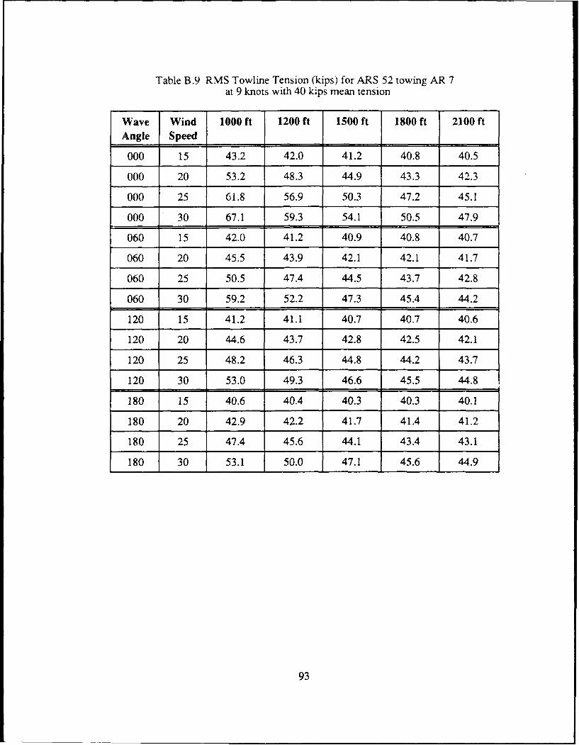
Table B.9 RMS Towline Tension (kips) for ARS 52 towing AR 7at 9 knots with 40 kips mean tension
Wave Wind 1000 ft 1200 ft 1500 ft 1800 ft 2100 ftAngle Speed
000 15 43.2 42.0 41.2 40.8 40.5
000 20 53.2 48.3 44.9 43.3 42.3
000 25 61.8 56.9 50.3 47.2 45.1
000 30 67.1 59.3 54.1 50.5 47.9
060 15 42.0 41.2 40.9 40.8 40.7
060 20 45.5 43.9 42.1 42.1 41.7
060 25 50.5 47.4 44.5 43.7 42.8
060 30 59.2 52.2 47.3 45.4 44.2
120 15 41.2 41.1 40.7 40.7 40.6
120 20 44.6 43.7 42.8 42.5 42.1
120 25 48.2 46.3 44.8 44.2 43.7
120 30 53.0 49.3 46.6 45.5 44.8
180 15 40.6 40.4 40.3 40.3 40.1
180 20 42.9 42.2 41.7 41.4 41.2
180 25 47.4 45.6 44.1 43.4 43.1
180 30 53.1 50.0 47.1 45.6 44.9
93

Table B.10 RMS Towline Tension (kips) for ARS 52 towing AR 7at 3 knots with 80 kips mean tension
Wave Wind 1000 ft 1200 ft 1500 ft 1800 ft 2100 ftAngle Speed
000 15 82.5 81.8 81.3 80.9 80.7
000 20 94.9 90.5 87.1 85.1 83.8
000 25 141.0 112.6 99.9 94.1 90.5
000 30 294.0 180.9 127.5 109.9 101.5
060 15 83.0 82.1 81.9 81.8 81.2
060 20 89.7 87.6 85.0 84.8 83.3
060 25 109.0 96.2 90.5 89.0 86.5
060 30 234.8 144.4 102.1 95.0 91.2
120 15 82.6 82.5 81.3 81.3 81.3
120 20 88.9 87.6 84.9 84.2 83.9
120 25 99.3 93.6 89.5 87.8 86.7
120 30 171.8 166.9 96.8 92.2 90.1
180 15 81.7 81.1 80.8 80.8 80.4
180 20 88.1 85.6 84.2 83.5 82.3
180 25 104.0 96.5 91.4 88.8 86.7
180 30 151.4 122.4 105.5 97.8 93.4
94
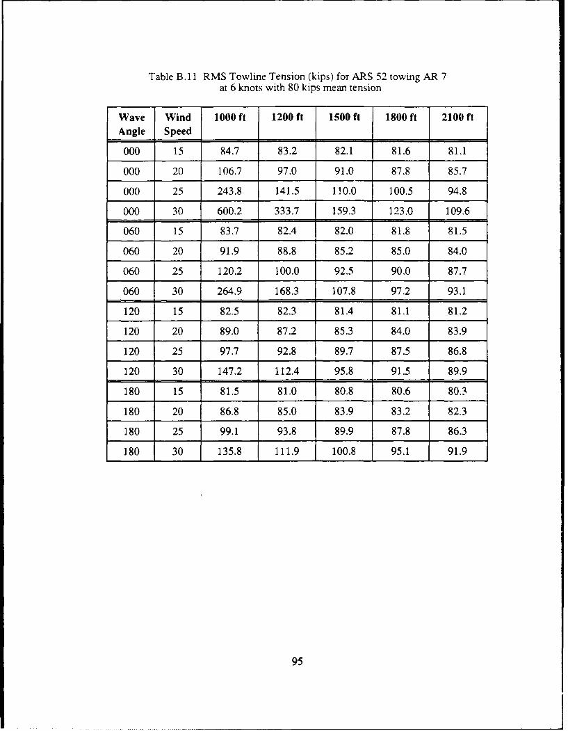
Table B. 1I RMS Towline Tension (kips) for ARS 52 towing AR 7at 6 knots with 80 kips mean tension
Wave Wind 1000 ft 1200 ft 1500 ft 1800 ft 2100 ftAngle Speed
000 15 84.7 83.2 82.1 81.6 81.1
000 20 106.7 97.0 91.0 87.8 85.7
000 25 243.8 141.5 1 10.0 100.5 94.8
000 30 600.2 333.7 159.3 123.0 109.6
060 15 83.7 82.4 82.0 81.8 81.5
060 20 91.9 88.8 85.2 85.0 84.0
060 25 120.2 100.0 92.5 90.0 87.7
060 30 264.9 168.3 107.8 97.2 93.1
120 15 82.5 82.3 81.4 81.1 81.2
120 20 89.0 87.2 85.3 84.0 83.9
120 25 97.7 92.8 89.7 87.5 86.8
120 30 147.2 112.4 95.8 91.5 89.9
180 15 81.5 81.0 80.8 80.6 80.3
180 20 86.8 85.0 83.9 83.2 82.3
180 25 99.1 93.8 89.9 87.8 86.3
180 30 135.8 111.9 100.8 95.1 91.9
95

Tat1 - B.12 RMS Towline Tension (kips) for ARS 52 towing AR 7at 9 knots with 80 kips mean tensio.
Wave Wind 1000 ft 1200 ft 1500 ft 1800 ft 2100 ftAngle Speed
000 15 91.5 86.7 84.1 83.0 81.8
000 20 150.9 114.0 99.6 93.2 89.1
000 25 383.5 263.7 133.6 112.6 102.6
000 30 719.9 761.2 285.0 150.4 123.6
060 15 84.8 83.2 82.0 81.9 81.8
060 20 95.4 90.9 86.8 85.5 84.9
060 25 169.8 110.1 95.6 91.6 89.2
060 30 301.4 203.2 115.1 100.3 95.5
120 15 82.4 82.0 81.4 81.0 81.1
120 20 89.0 86.9 85.6 84.0 83.9
120 25 97.0 92.3 89.9 87.5 86.9
120 30 132.6 120.2 95.2 91.1 89.7
180 15 81.3 80.9 80.7 80.5 80.2
180 20 86.1 84.7 83.5 82.9 82.4
180 25 96.7 92.5 89.2 87.3 86.3
180 30 123.7 106.2 98.2 93.6 91.2
96

1 50 -_____
140 Mean Tension130 -... 10 kips
120 -- - 9nots - -- 20 ips
110 6knots 4kips0 -3 knots100 - ,""80 kips
70
2E 60 -
o
30
20 ---
10 7. - . - - .- .- - - - - - - - - - - - - - - - - - - - - - - - - - - - - - - - - - - - - - - - - - - - - - - - - - - - - - - - -
0
1000 1200 1400 1600 1800 2000
Hawser Length (feet)
Figure B.I ARS 52 towing AR 7 on 2.25 inch wire hawserRelative Wave Angle 000, Wind Speed 15 knots
150 -
140 - Mean Tension130 - 9 knots ---- 10 kips
J2 / 6 knots~~9knots... 20ks
110 --- 40 kips7 80 kips
70
60
so0 - - -- - - - - - - - - -- - - - -
40
30-
20 -
0 o o I I I T1l00 1200 1400 1600 1800 2000
Hawser Length (feet)
Figure B.2 ARS 52 towing AR 7 on 2.25 inch wire hawserRelative Wave Angle 000, Wind Speed 20 knots
97
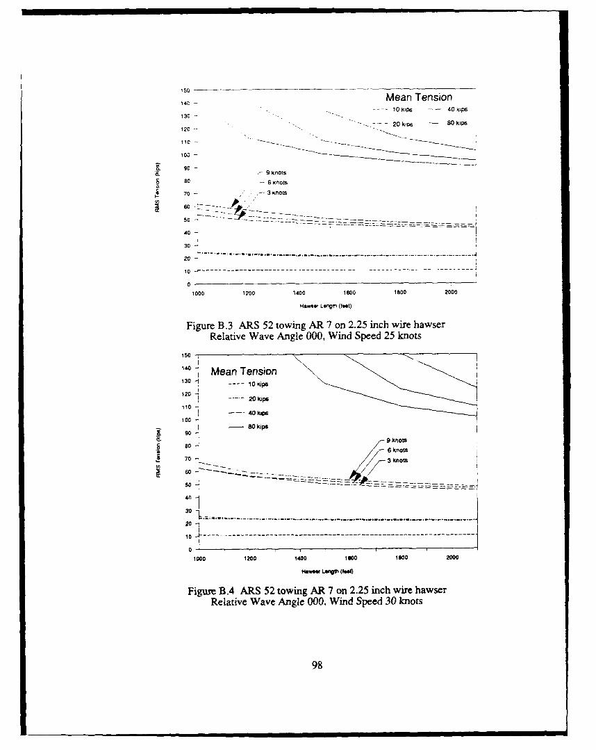
50 Mean Tension140
----- 10kips -- 40Kips130 -- -2
_ 20 kps 80 kips120
100 -
~ 90-9 Knots
80 - -K 6Knots
70 3 knots
50- - - - --- - - - Z-
40-
30 -
20 -
10 -' ...........................
0
1000 1200 1400 1600 1800 2000Hawser Lengo (leet)
Figure B,3 ARS 52 towing AR 7 on 2.25 inch wire hawserRelative Wave Angle 000, Wind Speed 25 knots
150,c Mean Tension
130 kis 1k
120 -
~9 k~nots
- i ,- 6 knotsi70 - 3 knots
, ik
30
20 ~ p
10 ..................................................................
100 1200 1400 1600 160o 2000
Haw.,,w LW (11"t)
Figure B.4 ARS 52 towing AR 7 on 2.25 inch wire hawserRelative Wave Angle 000, Wind Speed 30 knots
98

150
140 -- Mean Tension130 - ---- 10 kps
120 - --- 20 K PS9 knots
110 - 6Knot -- 40k1iP
100 - 7- 3Knots - 0kips
S 90 -
- -
70 -
U32 60 -
50 -
40 -
30 -
302 00 - -- ---. ................... ............................. ............... ......... ....
1 0 - -- -- -- -- -- -- - -- -- -- -- -- -- -- - -- -- -- -- -- -- -- -- -- -- -- -- -- -- -- - -- -- ---
D
1000 1200 1400 1600 1800 2000
Hawser Length (toot)
Figure B.5 ARS 52 towing AR 7 on 2.25 inch wire hawserRelative Wave Angle 060, Wind Speed 15 knots
150
140 - Mean Tension130-. 10 kips
1 F 9 knots120 6 knots 20kips
110, 3 3knots 40 kips
100 -S-80 kips
90-S so -
70-
60-570 -
30-
20
10
1000 1200 1400 1600 1800 2000
Mse-t Le4'VM (feet)
Figure B.6 ARS 52 towing AR 7 on 2.25 inch wire hawserRelative Wave Angle 060, Wind Speed 20 knots
99

ISO
150
140 - Mean Tension130 - 9 knots ---- 0 kips
-6 knots120 .3knots - - - 20 KIp6
110-"- - 40kip
80 kip6
so-
70-
2 60-
40 -
30 -
20
10 -- ----------------------------------..........................
0
1000 1200 1400 1600 1800 2000
Hawur Lengitl (fet)
Figure B.7 ARS 52 towing AR 7 on 2.25 inch wire hawserRelative Wave Angle 060, Wind Speed 25 knots
Mean Tension130 . kip
120 kips
110 So
100-
90-so , 9 knots
a 1 if 6 knots70 7 3 knots
40 _
30
1000 1200 1400 1600 1800 2000
HMw LarVM (f se)
Figure B.8 ARS 52 towing AR 7 on 2.25 inch wire hawserRelative Wave Angle 060, Wind Speed 30 knots
100
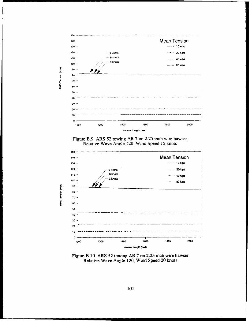
140 - Mean Tension130 - - -- 0KIPS
120 - 9 9Knots --- 20 ips
110 - 6 knots 40Okips
10 / 3 knots - 80 kips
70-
60-
50-
30
1000 1200 1400 1600 1800 2000
Hawser Length (feet)
Figure B.9 ARS 52 towing AR 7 on 2.25 inch wire hawserRelative Wave Angle 120, Wind Speed 154 knots
150
140 7 Mean Tension130 - -- - 0kips
120 9 - knots --- 20kips
110 -6 Knots 40 kip
100~ ~ / 3 knots 0kp
0
70-
50-
-------------------------------------------40-
30 -
20
10 -- - - - - - - - - - - - - - - - -- - - - - - - - - - - - - - - - - - - -- - - - -- - - --
01000 1200 1400 1600 1800 2000
Hae~ Lamm~ (bee)
Figure B.10 ARS 52 towing AR 7 on 2.25 inch wire hawserRelative Wave Angle 120, Wind Speed 20 knots
101

150
140 -Mean Tension
no - 9 Knots --- 10 KIPS
120 - - 6Knots - - - 20 kips3 knots
110 - -- 40kips
100 - kips
$ 80-
70-
50 -
40-
30-
20
10 -
0
1000 1200 1400 1600 1800 2000
Hawswf Length (ibot)
Figure B. 1I ARS 52 towing AR 7 on 2.25 inch wire hawserRelative Wave Angle 120, Wind Speed 25 knots
150
140 Mean Tension10 -9 knots ---- 10 kips
106
knotsM
120 -- 3 knots . .. 20 kips
10 1)
50 -
k .
70j50-J10
102
1 ----------------------------------------------

150
140 Mean Tension130 - ---- 10 KiPS
:20- - - - 20 Kips
9 knots110 - - 6 knots 40 kips
100 -"- 3 knotS - 80 Kips
g -/ /. 9 - ppp80 -
70 - 7
50 -.
30 -200 . ............. ................. ................. .......... ....... ........... .....
1 0 . . . . . . . . . . . . . . . . . . . . . . . . . . . . . . . . . . . . . . . . . . . . . .
0
1000 1200 1400 1600 1800 2000
Haw er L~nI t 1oot)
Figure B. 13 ARS 52 towing AR 7 on 2.25 inch wire hawserRelative Wave Angle 180, Wind Speed 15 knots
150
140 Mean Tension130 -- .... 10 kips
120 -9 - knots . .. 20kip;
6 knots 40 kips10"//
3 knots100- 80 kips
g o
70 -
soir
40-"
307
20 - - - - -
10 ,
0
1000 1200 1400 1800 1800 2000
Hawser Lmth (f-t)
Figure B.14 ARS 52 towing AR 7 on 2.25 inch wire hawserRelative Wave Angle 180, Wind Speed 20 knots
103

14 Mean Tension13C - 9 Knoats -- 0KD
120 - 3 kn1ots 20 K2ivps
110 - -- 40 kips
l00
80 kips
90-
80-
50-
40-
30
0
1000 1200 1400 1600 1800 2000
Hawser Length (feet)
Figure B. 15 ARS 52 towing AR 7 on 2.25 inch wire hawserRelative Wave Angle 180, Wind Speed 25 knots
Mean Tension
130 r
30 kip120 3 kot
100 420 1k0ip0s80 20
710

Appendix C
Test Plan
105
NAVSEA TWO BODY TOWING EXPERIMENT
TEST PLAN
REVISION 1
LT E.N. Christensen, USN
Protessor J.H. Milgram
Dr. F.C. Frimm
Department of Ocean Engineering
Massachusetts Institute of Technology
26 April 1989

TEST PLAN - NAVSEA TWO BODY TOWING EXPERI1MNT
Chapter One
Experiment Overview
1.1 Objective
The theory for extreme towline tension statistics, developed at MIT, now forms the
basis for the prediction of dynamic towline loadings experienced during open ocean towing
in the U.S. Navy Towing Manual (1988). Although it is the most advanced theory currently
available, it has not been validated by full-scale experiment at sea. The Two Body Towing
Experiment, sponsored by the Supervisor of Salvage and Diving (NAVSEA OOC), is
designed to assess the validity and applicability of this analytical method.
The Two Body Towing Experiment has been devised to acquire a large quantity of
high quality data to help determine the influence of ship characteristics and environmental
conditions on the dynamic tensions developed during open ocean towing. Post-voyage anal-
ysis will produce a thorough comparison to analytical predictions. It is hoped that the results
of this experiment will provide a better understanding of the nature of dynamic loadings
107

TFS1 PLAN - NAVSEA TV O BODY TOWING EXPERIMENT
which will allow better accuracy in predicting extreme tensions. This will not only help to
improve towing safety and give operators greater confidence to tow at higher speeds \ !n
dynamic tensions are low, but perhaps allow for a reduction of the traditional factors of
safety used in open ocean towing.
1.2 Participating Organizations
The Two Body Towing Experiment structural organization is shown in figure 1.1. The
Supervisor of Salvage and Diving (NAVSEA OOC) is the test sponsor. The following is a
summary of the organizations supporting the test and their individual responsibilities:
Department of Ocean Engineering, Massachusetts Institute of Technology (MIT):
Responsible for overall direction for test planning, conduct of operations, and datameasurement. Provide data acquisition computer with software and laser rangefinder.
POC: LT Erik Christensen (617) 253-5890Dr. Fernando Frimm (617) 253-5191Professor. Jerome Milgram (617) 253-5943
ARCTEC Offshore Corporation (AOC):
Provide and install all sensors and signal conditioning equipment and assign a fieldelectronics technician during the testing phase.
POC: Mr. Peter Zahn (301) 730-1030
USS SALVOR (ARS 52):
Provide towing services in addition to logistic support services as noted in sections5.3 and 5.4.
POC: LCDR Bob Reish (808) 471-0123
108
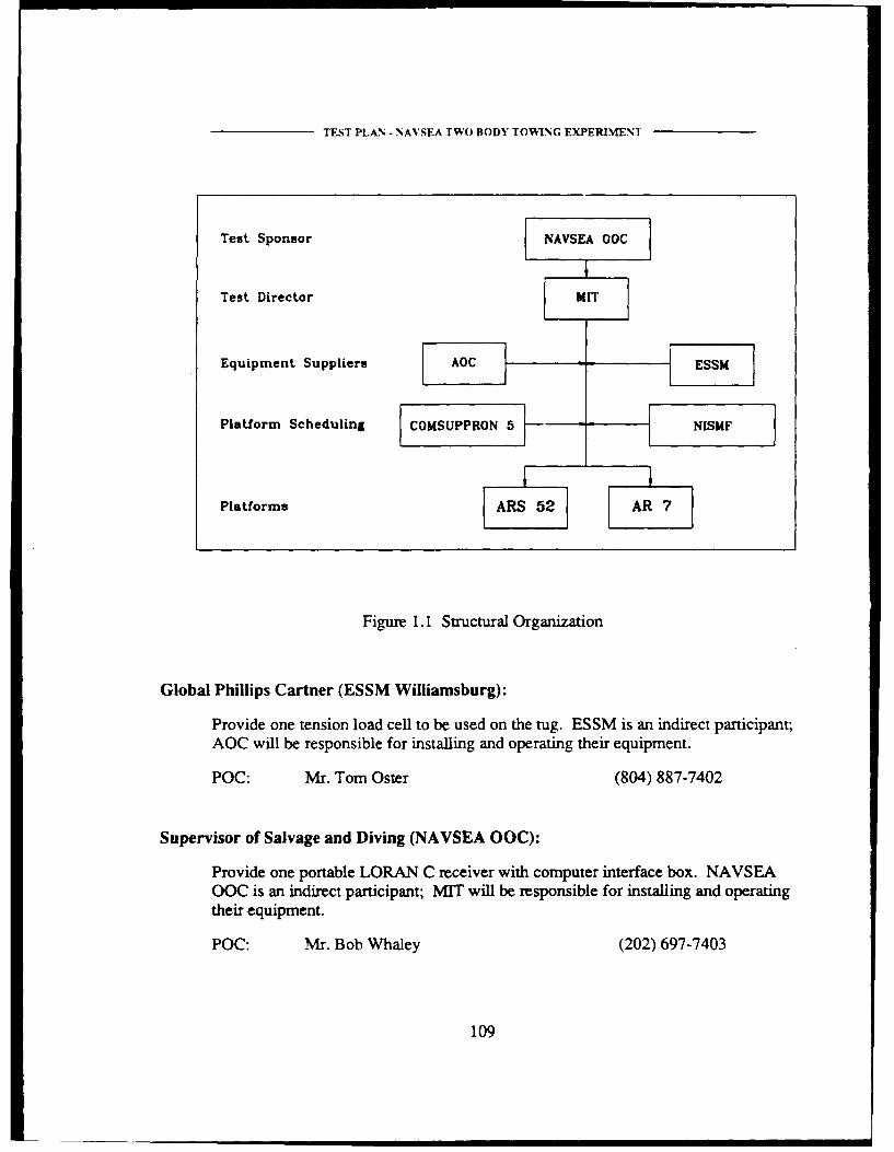
TEST PLAN - NAVSEA TWO BODY TOWING EXPERIMENI
Test Sponsor NAVSEA OOC
I
Test Director MIT
Equipment Suppliers AOC ESSM
Platform Scheduling CObSUPPRON 5 NISMF
Platforms ARS62 ARE
Figure 1.1 Structural Organization
Global Phillips Cartner (ESSM Williamsburg):
Provide one tension load cell to be used on the tug. ESSM is an indirect participant;AOC will be responsible for installing and operating their equipment.
POC: Mr. Tom Oster (804) 887-7402
Supervisor of Salvage and Diving (NAVSEA 00):
Provide one portable LORAN C receiver with computer interface box. NAVSEAOOC is an indirect participant; MrI will be responsible for installing and operatingtheir equipment.
POC: Mr. Bob Whaley (202) 697-7403
109

TEST PLAN - NAVSEA TWO BODY TOWING EXPERIMENT
Commander, Support Squadron 5 (COMSUPPRON 5):
Schedule a tug for the experiment.
POC: LT Karen Kohanowich (808) 474-7769
Inactive Ship Maintenance Facility, Pearl Harbor, HI (NISMF):
Provide the ex-USS HECTOR (AR 7) configured with a towing bridle.
POC: Mr. Lee Cobb (808) 471-4547
1.3 Test Platforms
The characteristics of the two platforms participating in the test are shown in Table 1.1
and described below.
Table 1.1 Gross Characteristics of Test Platforms
TUG TOW
Ship ARS 52 AR 7
Length (ft) 255 520
Beam (ft) 52 73
Draft (ft) 15.5 15.5
Displacement (Ltons) 2,850 10,130
110

TEST PLAN - NAVSEA TWO BODY TOWING EXPERIMENT
1.3.1 Tug
The USS SALVOR (ARS 52) is a "Safeguard" Class Salvage ship. Commissioned on
14 June 1986, the SALVOR is a member of the newest class of salvage ship in the U.S. Navy
inventory. She is powered by four Caterpillar D-399 diesel engines which produce a total of
4200 SHP. The SALVOR has an Almond A. Johnson Series 322 automatic towing machine
which holds 3000 feet of 2.25 inch wire towing hawser and has a traction winch for 14 inch
fiber rope hawsers. The SALVOR is capable of producing 138,000 pounds of bollard pull
thrust.
1.3.2 Tow
The ex-USS HECTOR (AR-7) is a "Vulcan" Class Repair Ship commissioned on 7
February 1944. She was recently decommissioned from the U.S. Navy inventory and is in
the process of being leased to the Pakistani Navy through the Foreign Military Sales Pro-
gram. The HECTOR is currently in the custody of the Inactive Ship Maintenance Facility,
Pearl Harbor, Hawaii. Permission has been obtained from the Office of the Chief of Naval
Operations (CNO) to use the HECTOR prior to that transfer.
111

TEST PLAN - NAVSEA TWO BODY TOWING EXPERIMENT
Chapter Two
Data Products
2.1 Data Collection
Data collection will focus on tension measurements using two tension sensing load
cells with simultaneous measurement of various parameters affecting dynamic tension
extremes. All data is to be collected at one data acquisition site in digitized form and
recorded on diskettes compatible with the IBM-PC standard to allow immediate playback
and complete post-voyage analysis. Table 2.1 shows all parameters that will be simulta-
neously recorded on the primary data acquisition system computer. As an additional measure
of redundancy and to provide a quick means of verifying recorded data, the output from
various installed shipboard sensors will be manually recorded. It is requested that tug per-
sonnel assist in the data collection effort by manually recording the data shown in table 2.2
and as noted in section 5.3. Enclosure (1) is provided to assist in this effort.
112

TEST PLAN - NAVSEA TWO BODY TOWING EXPERIMENT
Table 2.1 Primary Data Collection
PARAMETER LOCATION INSTRUMENT
Wind Speed tug portable anemometer
Wind Direction tug portable wind vane
Heading tug, tow flux gate compass
Hawser Tension tug, tow tension link
Hawser Angle tug, tow hawser angle indicator
Surge tug, tow 6 DOF motions package
Sway tug, tow 6 DOF motions package
Heave tug, tow 6 DOF motions package
Roll tug, tow 6 DOF motions package
Pitch tug, tow 6 DOF motions package
Yaw tug, tow 6 DOF motions package
Wave Height tug Doppler radar sensor
Speed tug LORAN receiver
Range tug laser range finder
2.2 Instrumentation
The instrumentation to be used during the Two Body Towing Experiment is summarized
in figure 2.1 and discussed below. All measurements made on the tug will be directly cou-
pled to the primary data acquisition unit using coaxial cables. A redundancy in the recording
of all measurements is desirable and considered necessary to provide a measure of safety in
113

TEST PLAN - NAVSEA TWO BODY TOWING EXPERIMENT
Table 2.2 Manual Data Collection
PARAMETER INSTRUMENT FREQUENCY
Wind Speed installed sensor 10 minutes
Wind Direction installed sensor 10 minutes
Ship's Position LORAN, SATNAV, visual 10 minutes
SOG LORAN, SATNAV, visual 10 minutes
COG LORAN, SATNAV, visual 10 minutes
Speed installed sensor 10 minutes
Wave Height seaman's eye hourly
Hawser Length visual all changes
Shaft rpm installed sensor all changes
Propeller Pitch installed sensor all changes
Ordered Course --- all changes
Ordered Speed --- all changes
the event of data transmission problems. Therefore, all measurements made on the tow will
be recorded locally on a personal computer and simultaneously telemetered to the tug via an
FM telemetry system. Software routines will allow active monitoring of all measurements on
a real-time basis and provide online comparison to analytical predictions to assess the valid-
ity of recorded data.
2.2.1 Wind
A portable anemometer and wind direction vane will be manually installed on the tug by
AOC personnel. The most important aspect of wind measurement is the sensor location: the
114

TEST PLAN - NAVSEA TWO BODY TOWING EXPERIMENT
@9
9
TUG TOWI Anemometer and Wind Vane t2 Flux Gate Compes2 Fliux Gate Compam 13 Clevis Pin Tension Link3 Loran Receiver t4 Pitch Accelerometer4 Laser Range Finder t5 Yaw Accelerometer6 Hawer Angle Indicator 16 Surge. Sway. Heave Accelerometers6 Doppler Radar Sensor 17 Roll Accelerometer7 PItch Accelerometer8 Yaw Accelerometer9 Surue. Swey, Heave Accelerometer10 Roll Accelerometeri1 Tension Link
Figure 2.1 Sensor Location
unit must be installed in a position that is unobstructed from all directions. This will require
that the unit be placed high on top of one of the masts such that it is above wind separation
regions in all directions. The output will be wired directly to the data acquisition computer.
To maintain redundancy in the data collection effort and to provide a means of quick cross
check reference, both the wind speed and direction, as indicated on the ship's installed sen-
sors, will be manually recorded every ten minutes by ship's personnel.
115

TEST PLAN - NAVSEA TWO BODY TOWING EXPERIMENT
2.2.2 Ship Speed
A portable LORAN C receiver will be installed on the tug by MIT personnel. The unit
will provide both a digital readout of latitude and longitude and an RS-232 computer output
for direct recording of information onto the data acquisition computer. To maintain redun-
dancy and provide a quick cross check reference, the speed indication from the ship's
installed speed log and computations of speed over ground (SOG) between successive
navigation fixes will be recorded manually every ten minutes.
2.2.3 Wave Height
A portable Doppler radar sensor will be mounted on a metal pipe extending approxi-
mately ten feet forward of the bow of the tug. The unit will measure the Doppler shift of a
microwave radar emission that is bounced off the sea surface. The motions of the ship will
be decoupled from the data through an internal gyroscopes. The output signal will be con-
nected directly to the data acquisition computer. To maintain redundancy in the data collec-
tion effort and to allow a means of quick cross check reference, a visual estimate of the wave
height, based on an experienced "seaman's eye," will be manually recorded at the start and
completion of each test run by ship's personnel. As the ship pitches and rolls and travels
through the water it radiates energy into the water in the form of waves. Unless an on-site
calibration procedure is performed, the influence of these ship generated waves can severely
corrupt wave height measurements. The calibration of this sensor involves comparison of
data measured in the vicinity of a "reference" wave height sensor. Chapter 6 provides addi-
tional information and details on performing this calibration.
116
TEST PLAN - NAVSEA TWO BODY TOWING EXPEIMENT
2.2.4 Motions
A six degree of freedom (DOF) motion sensing package will be installed on both the
tug and the tow by AOC personnel. The main unit, consisting of a vertical referenced gyro-
scope and three accelerometers, will be mounted near the ships center of gravity (CG) and
used to measure translational motions (surge, sway, and heave.) Three other servo
accelerometers, each enclosed in individual weather-tight containers, will be mounted at
known locations from the main unit and measure rotational motions (roll, pitch, and yaw.)
On the tow, all accelerometers will be wired to a data recorder and FM telemetry system. On
the tug, all accelerometers will be wired directly to the main data acquisition unit.
2.2.5 Heading
Portable flux gate compasses will be mounted on both the tug and tow to provide a
continuous record of the dynamic, time-varying heading of both vessels. Since the compass
is sensitive to magnetic fields, any magnetic disturbance near it cause a deflection from the
proper reading. To minimize the effects of residual magnetism of the ship, the flux gate
compass should be installed in a spot where the magnetic field is uniform so that the local
magnetic field lines will only change slowly; as far as possible from the nearest metal surface
in a location which does not have sharp edges or comers which could cause the field direc-
tion to change rapidly. The optimum location for installation of these units will have to be
determined after an on-site inspection. The output from these will be sent directly to the
main data acquisition computer. To compensate for the errors produced by the ship's mag-
netic signature, both compasses must be calibrated after installation and their deviation com-
puted. This will require that both vessels be "swung" so that the indicated magnetic heading
117

TEST PLAN - NAVSEA TWO BODY TOWING EXPERIMENT
on the flux gate compasses can be compared to the installed magnetic compass on board the
tug for various courses. Chapter 6 provides additional information and guidelines for con-
ducting this procedure.
2.2.6 Tension
Strain gaged tension links will be used to measure the dynamic tensions developed at
both ends of the hawser. On the tug, the tension will be measured from a 160 kip load cell
attached to the hawser using a carpenter stopper as shown in figure 2.2. Installation will be
performed by AOC with assistance from the crew of the tug. Coaxial cable will run directly
from the tension link to the data acquisition unit. Since the towing load will be taken up by
the load cell, the ship's installed tensiometer will be inoperative during testing. On the tow,
tension will be measured from a 180 kip waterproof load cell mounted in a clevis pin con-
nected to the flounder plate of the towing bridle as shown in figure 2.3. Data will be
recorded locally and telemetered to the main data acquisition unit.
118

TEST PLAN - NAVSEA TWO BODY TOWING EXPER NNT
DECK PADEY[
SAFETY SHAZKLE WIRE PENDANT
TENSION LINK
SAFETY SHACKLE
CARPENTER STOPPER -
• .- TOW HAWSER
Figure 2.2 Tug Towing Configuration
2.2.7 Range
The distance between the two vessels will be continuously measured using a handheld
laser range finder. The unit is approximately the size of a large pair of binoculars (11.4" x
9.4" x ".3"), weighs 8.2 pounds, and is powered by normal ship's power (120 VAC). It will
be mounted on a tripod and manually trained on a reflector positioned on the bow of the tow
using an integrated telescopic lens. Distance is simultaneously displayed in the view finder
and output directly into the data acquisition unit via coaxial cable.
119

TEST PLAN- NAVSEA TWO BODY TOWING EXPERIMEN'I
CHAIN RR:DE
- -DETAC-iABLE LIM,~
--- PLA-E SI ACKLE
FLOUNDER PATE
.LEVIS PIN
WIRE[ P[ NIAN-
PLATE SHACKLE -
,,--- DETACHAB.E LINK
CHAIN PENDANT
Figure 2.3 Towing Bridle Configuration
2.2.8 Hawser Angle
The towing hawser azimuth angle indicators will be installed on the fantail of the SAL-
VOR and on the bow of the HECTOR by AOC personnel. These indicators use string poten-
tiometers to measure the vertical and horizontal angular displacement of the towline.
120

TEST PLAN - NAVSEA TWO BODY TOWING EXPERI.MENT
2.2.9 Hawser Length
The exact length of towing hawser is to be measured by visual verification as it is paid
out from the towing machine. Using a known length, such as the distance from the towing
H-bits to the stem roller, the towing machine operator can record the number of lengths of
cable subsequently paid out or taken up. Comparison with the installed shipboard sensor
should be done for redundancy.
121

TEST PLAN - NAVSFA TWO BODY TOW1NG EXPERIMENT
Chapter Three
Schedules
3.1 General Test Schedule
Table 3.1 provides a schedule of major events for this exercise.
Table 3.1 SCHEDULE OF EVENTS
DATE LOCATION SHIP EVENT
May 4 - 7 inport AR 7 * sensor installation
May 8 - 9 inport ARS 52 * sensor installation
May 10 - 12 at sea ARS 52 * calibration procedures
May 13 - 14 inport ARS 52 & AR 7 • system verification
1 dry run test of all sensors
May 15 - 18 at sea ARS 52 & AR 7 e wire rope data collection
May 19 at sea ARS 52 & AR 7 • fiber rope data collection
May 20 - 22 inport ARS 52 & AR 7 • demobilization
122

TEST PLAN- NAVSEA TWO BODY TOWING EXPEIMIENT
3.2 Sensor Installation
The installation of sensors, as shown in figure 2.1, will occur inport during the period
May 4 - 9. AOC will be responsible for the majority of the instrumentation and will have a
small contingency of technicians available to perform this work. It is requested that they be
given free access to both ships while installing equipment.
3.3 At-sea Calibration
The initial at-sea period will be used for calibration of the wave height sensor and the
flux gate compass. Only the SALVOR is required for this procedure. The details of con-
ducting the calibration are provided in chapter 6. Upon returning to port from this phase, it is
requested that the SALVOR moor in close proximity to the HECTOR to assist in the system
N erification procedures.
3.4 System Verification
Although the at-sea calibration procedure will afford the opportunity of verifying many
of the sensors installed on the tug, a complete end-to-end test of all sensors must be per-
formed before commencing the experiment. The total data acquisition and instrumentation
lineup will be verified with data from all sensors being simultaneously recorded during the
period May 13 - 14.
123

TEST PLAN - NAVSEA TWO BODY TOWING EXPERIMENT
3.5 At-sea Data Collection
The daily test schedule is outlined in table 3.2 and described below. Primarily for per-
sonnel safety, the test is only to be conducted during daylight hours. Preparations will com-
mence at 0700 daily when the length of towing hawser will be verified and both the hawser
angle indicator and the deck tension link will be reinstalled with assistance from the ship's
crew. A small boat, provided by the SALVOR, will be used to ferry the technician to the
tow. Once on the tow, the technician will start up the portable generator and energize all
transducers and signal conditioning equipment. The data acquisition station operator on the
tug will visually verify receipt of all local and telemetered signals before the actual data col-
lection will commence.
After confirming that all transducers are operational, the experiment supervisor will
inform the Officer of the Deck (OOD) that data recording is ready to commence. Each seg-
ment of uninterrupted data collection should last approximately 30 to 45 minutes. The
experiment supervisor will inform the OOD upon completion of each segment of the
experiment.
Upon completion of each day's data collection, at approximately 1900, the technician
on the tow will de-energize all equipment and a small boat will ferry him to the tug. On the
tug, all transducers and signal conditioners will be de-energized and the data collection sheets
will be collected from the ship bridge team. Each evening, an analysis of all sampled data
will be conducted to reconfirn the validity of all recorded data. The towing experiment
124

TEST PLAN - NAVSEA TWO BODY TOWING EXPERIMENT
supervisor will inform the Commanding Officer and ship's navigator of the requested sea
conditions for the following day's data collection so that appropriate navigational tracks can
be laid out.
3.6 Demobilization
The last two days of the experiment will be used to remove all sensors from both ves-
sels and prepare the instruments for shipment back to their parent organizations. Initial
demobilization can begin while at sea upon completion of data collection.
3.7 Contingency Plans
In the event of equipment malfunction or deteriorating weather conditions, modifica-
tion to the events in this schedule will be made on a case-by-case basis. A conscious effort
has been made to ensure sufficient redundancy in recording of data to minimize the effects of
equipment failure. Since the vast majority of equipment is to be provided by AOC, the pres-
ence of one of their electronic technicians, who is familiar will all sensors used, is considered
very prudent. In addition, both MIT and AOC will have a quantity of spare parts on hand to
allow at-sea replacement rather than requiring assistance from ashore.
125
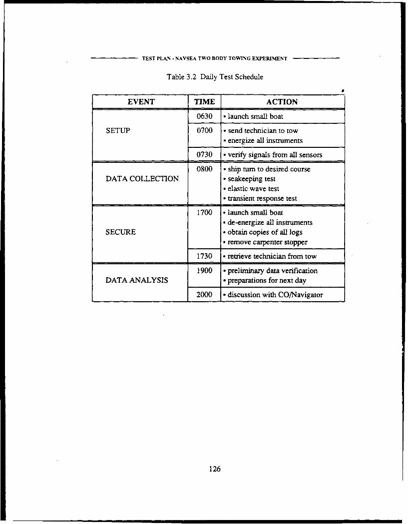
TEST PLAN - NAVSEA TWO BODY TOWING EXPERIMENT
Table 3.2 Daily Test Schedule
EVENT TIME ACTION
0630 • launch small boat
SETUP 0700 • send technician to tow- energize all instruments
0730 • verify signals from all sensors
0800 • ship turn to desired courseDATA COLLECTION * seakeeping test
* elastic wave test- transient response test
1700 • launch small boat* de-energize all instruments
SECURE - obtain copies of all logse remove carpenter stopper
1730 - retrieve technician from tow
1900 - preliminary data verificationDATA ANALYSIS - preparations for next day
2000 - discussion with CO/Navigator
126

TEST PLAN - NAVSEA TWO BODY TOWING EXPERIMENT
Chapter Four
Tow Test
4.1 Overview
The primary purpose of this experiment is to measure the dynamic tensions developed
in a wire towing hawser while towing in the open ocean. By measuring all factors that influ-
ence towline tension, the analytical models can be verified step-by-step. A series of seakeep-
ing tests have been designed to accomplish this. In addition, four other tests have been
developed to supplement the data collection effort. This will provide a wealth of information
for post voyage analysis. However, at no time should the successful completion of the sea-
keeping test be jeopardized by the accomplishment of any of these secondary tests.
4.1.1 Seakeeping Test
GOAL: to assess the validity of current analytical models in predicting tension
extremes and ship response to environmental conditions during towing.
PROCEDURE: A series of test runs will be performed varying a different parameter each
time. Ideally, the test should be performed in two different sea states with
127

TEST PLAN - NAVSEA TWO BODY TOWING EXPERIMENT
four towing angles, three towline lengths at two different speeds. How-
ever, this would require a total of 48 test runs which would take well in
excess of one week of at-sea measurement. Acceptable results can be
obtained by conducting only a select portion of these provided that each
parameter is varied sufficiently to identify trends and allow correlation
with analytical predictions. Each test run should be done at constant
speed and heading with data recorded continuously for 30 to 45 minutes.
The first five minutes of each run will be used to verify that all sensors
are operating correctly. The individual ship headings will be determined
based upon local conditions to obtain the proper angle with respect to the
waves during data recording. It is requested that the tug only maneuver
as necessary to avoid navigation hazards or other shipping. Should the
ship be required to maneuver during data collection, the experiment will
be halted and that portion repeated. During each test run, the data acqui-
sition team will monitor and record all parameters shown in table 2.1. To
maintain redundancy in the data collection effort and to allow a means of
quick cross check reference, it is requested that the SALVOR's naviga-
tion team manually monitor and record the parameters shown in table 2.2
using enclosure (1).
4.1.2 Towing Machine Test
GOAL: to measure the dynamic response of the towing machine while towing in
the automatic mode.
PROCEDURE: Conduct one of the seakeeping tests, as discussed above, with the towing
machine in the automatic mode. By adjusting the pay out release tension
on the towing machine to a value just above the predicted RMS tension
value for the specific scenario, the towing machine should automatically
128

TEST PLAN - NAVSEA TWO BODY TOWING EXPERIMENT
pay out and retrieve the towing hawser as the dynamic tensions fluctuate
above and below the preset limits. Since the carpenter stopper cannot be
used on the fantail of the tug to connect the tension link to the towing
hawser, all tension measurements will be made from the tow end of the
hawser. If possible, the electrical signal to the ship's tensiometer will be
recorded along with the drum position. Immediately following this test,
reinstall the carpenter stopper and repeat the test with the same condi-
tions.
4.1.3 Fiber Rope Test
GOAL: to assess the validity of current analytical models in predicting the tension
extremes developed while towing with synthetic (fiber) towing hawsers.
PROCEDURE: Conduct several seakeeping tests, as discussed above, while towing on a
fiber towline. This is planned for the last day of the at-sea data collection
period. Initially, the tow will have to brought into "short stay" so that the
chain pendant at the end of the wire towing hawser is retrieved on the
fantail of the SALVOR. The wire hawser is to be removed and a 14 inch
fiber towline is to connected to the chain pendant then streamed astern.
These tests should be conducted at two different speeds (6 and 9 knots)
and two different lengths (1000 and 1500 ft).
4.1.4 Elastic Wave Test
GOAL: to attempt to determine if elastic waves are present and, if so, to measure
and record their existence. If excited at sufficiently high frequency, a
cable may develop elastic waves which may not be visible by the naked
eye. An evaluation of any elastic wave data collected will be performed
in post-voyage analysis.
129

TEST PLAN - NAVSEA TWO BODY TOWING EXPERIMENT
PROCEDURE: The elastic wave test is to be conducted for a total of five minutes imnime-
diately following with the seakeeping test. The only change from the
seakeeping test will be to raise the sampling frequency to 10 Hz and
increase the cutoff frequency to 3.3 Hz. It is requested that the SALVOR
continue on the specified test run track and continue monitoring parame-
ters as with the seakeeping test.
4.1.5 Transient Response Test
GOAL: to measure and record the response of the towing system during speed
changes.
PROCEDURE: Starting from just bare steerage, the ship's propeller pitch setting is to be
increased to pre-determined settings to yield final speeds of 3, 6, and 9
knots. Data should be collected continuously for six minutes at each
speed. The transient response test should be done in calm water (signifi-
cant wave height less than two feet) at three different towline lengths
(1000, 1500, and 2100 feet) at the conclusion of the seakeeping and
elastic wave tests. All data recording will be performed by the data
acquisition team.
4.2 Conduct of the Tests
The most labor intensive aspect of changing the towing configuration between succes-
sive runs is changing the length of the towing hawser paid out since it will require manual
resetting of carpenter stopper, careful measurement of hawser scope, and realignment of
hawser angle indicators. Therefore, it is recommended that initially, the hawser length be
kept constant and the other parameters (speed, sea state, and relative wave angle) be varied.
130

TEST PLA-N NAVSEA TWO BODY TOWING EXPERIMENT
Table 4.1 provides a tentative sequence of events to minimize labor between runs. Local
environmental conditions will dictate the optimal sequence and may require significant
changes to the proposed testing order. The test supervisor will rely heavily on the experience
of the Commanding Officer and navigation team to select the optimum locations for the
experiment. Three different lengths (1000, 1500, and 2100 ft), two different speeds (3 and 9
knots), and two different sea states (sea states 3 and 5) are to be investigated. In addition, the
influence of different wave angles will be considered.
During open ocean towing, it is standard practice to regularly "freshen the nip." This
involves shifting the point of contact of the towing hawser on the stem roller to minimize
wear by either paying out or hauling in the towing hawser a few feet. It is requested that no
such adjustments be made during data collection periods (0700 to 1900) as this would cause
excessive delays in the experiment as it would necessitate a readjustment of the carpenter
stopper and towing hawser angle indicator and careful measurement of the scope paid out.
4.3 Safety Precautions
As with all towing operations, one of the major safety concerns is the parting of the
hawser while under tension. Since the bollard pull of the SALVOR is rated at 138 kips and
the rated breaking strength of its 2.25 inch towing hawser is 444 kips (U.S. Navy Towing
Maua, 1988), the likelihood of hawser breakage during this experiment is small. However,
since dynamic tension surges can far exceed normal towing tensions, the possibility hawser
breakage cannot be completely dismissed. Since tensions will be continuously monitored by
the data acquisition computer operator, precautionary measures shall be taken if tensions
exceed predictions.
131
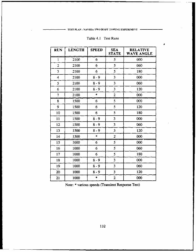
TEST PLAN- NAVSEA TWO BODY TOWING EXPERI.[EN-T
Table 4.1 Test Runs
RUN LENGTH SPEED SEA RELATIVESTATE WAVE ANGLE
1 2100 6 5 000
2 2100 6 5 060
3 2100 6 5 180
4 2100 8-9 3 000
5 2100 8-9 3 060
6 2100 8-9 3 120
7 2100 * 2 000
8 1500 6 5 000
9 1500 6 5 120
10 1500 6 5 180
11 1500 8-9 3 000
12 1500 8-9 3 060
13 1500 8-9 3 120
14 1500 * 2 000
15 1000 6 5 000
16 1000 6 5 060
17 1000 6 5 180
18 1000 8-9 3 000
19 1000 8-9 3 060
20 1000 8-9 3 120
21 1000 * 2 000
Note: * various speeds (Transient Response Test)
132

TEST PLAN - NAVSEA TWO BODY TOWING EXPERIMENT
Primarily for personnel safety, the Two Body Towing Experiment will only be con-
ducted during daylight hours. As an added precaution, it is requested that all personnel not
directly involved with the towing experiment be restrained from the fantail during the
experiment.
Except in emergency towing, it is normal U.S. Navy practice to tow only unmanned
tows. However, it is highly desirable to have a technician on the tow for the duration of each
day of towing to monitor the operation of all sensors and make immediate on-the-spot correc-
tions. In the event of rough seas making it unsafe to board or keep the tow manned, it is
requested that the ship maneuver to a calm region just long enough to allow the technician to
safely board the tow and energize all equipment. The tug can then tow the unmanned vessel
into rougher waters for data measurement.
133
TEST PLAN -NAVSEA TWO BODY TOWING EXPERIMENT
Chapter Five
Logistic Support
5.1 Navigation
No specific operating area (OPAREA) has been designated for this experiment. How-
ever, in order to achieve meaningful results, the wind speed and seas must be sufficient mag-
nitude to create dynamic tensions large enough for proper data analysis. Based on analytical
studies and previous experimental results, wind speeds greater than 15 knots and wave
heights greater than four feet are required. Each individual data collection phase of the
experiment will require the ship to maintain course and speed for approximately 45 minutes
while data is recorded. At all times, it is highly desirable to operate in regions away from
major shipping lanes to reduce the probability of having to adjust course or speed during a
data run.
134

TEST PLAN - NAVSEA TWO BODY TOWING EXPERIMENT
5.2 Communications
Two separate communication channels should be used in this experiment: one dedi-
cated to continuous data telemetry from tug to tow and the second for the test participants to
use for technical discussions and boat handling. AOC will provide a 14 channel FM-FM
telemetry system operating a frequency of 259 MHz. It is requested that the tug provide a
means of VHF cc-nmunications for the technical discussions and boat handling.
5.3 Data Collection
To assist with the interpretation of test results, the SALVOR is requested to manually
record the following data items. A sample data collection worksheet is provided in enclosure
(1) to assist in this effort.
1. Navigation Data
a. Log vessel's position at the begining, end, and every ten minutes during datacollection using, in order of preference, SATNAV, visual, or dead reckoning(DR) fixes.
b. Log all speed and course changes.
2. Ship Operating Conditions
a. Log the rpm of both shafts during each run.
b. Log the pitch settings of both propellers during each run.
c. Log the ship's speed, as read from the installed speed log, every ten minutes
135

TESI PLAN - NAVSEA TWO BODY TOWING EXPERIMENT
3. Environmental Data
a. Log wind speed and direction, as read from installed shipboard sensors,every ten minutes.
b. Log an estimate of the wave height, using seaman's eye, at the beginningand end of each data run.
4. Towing Hawser Log
a. Provide a copy of towing hawser log entries for each day of testing. Duringtesting, the load will be taken up by the tension link used in the experimentand so the shipboard tensiometer will not be operational. The experimentsupervisor can provide the towing machine operator with tension measure-ments as required for entry into the towing hawser log.
5.4 Support Services
During the at sea portion of the experiment, it is requested that the SALVOR provide
the following support items:
1. Assist in locating desirable areas of higher wind speeds and minimal traffic toconduct each day's testing. The experiment supervisor will provide specificrequests to the navigator and commanding officer each night after review andanalysis of collected data.
2. Supply one small boat (Whaler or ZODIAC type) and operator to transport a tech-nician to and from the tow daily as needed. During all data collection periods, itis highly desirable to have one person on board the tow to monitor the sensors andensure data is being recorded locally. Since no power will be available on thetow, all equipment placed on board will be powered by a portable generatorinstalled and operated by AOC.
3. Provide berthing and messing for three test participants; test director, test conduc-tor, and technician.
136

TEST PLAN - NAVSEA TWO BODY TOW"ING EXPERIMENT
4. Provide a dedicated location inside the ship, preferably near the fantail, with a
table and desk to install a data acquisition system consisting of two personal com-puters (IBM PC), monitors, keyboards, portable LORAN receiver, and FM telem-etry receiver. All data collected on the tug will be connected to the dataacquisition system using coaxial cables. Each night, preliminary data analysisand verification will be conducted here.
5. Provide an accurate measure of the amount of towing cable paid out past the sternof the tug. Although the installed shipboard sensor can be used, its accuracy can-not be guaranteed without conducting a calibration procedure. Instead, the pri-mary means of measuring the length of towing hawser paid out will be by visualmeasurement as described in section 2.2.9.
6. Provide a copy of the current deviation table for the magnetic compass installedon the bridge of the tug. This will be used as the reference for the determinationof the deviation of the portable flux gate compasses during the swing ship proce-dure.
7. Provide one carpenter stopper, wire rope pennant and safety shackles to connectthe hawser as shown in figure 2.3. It is requested that the tug provide manpowerassistance in riggin- this stopper during the experiment. It must be removedwhenever the length of cable is changed or when the ship "freshens the nip".Whenever installed, the shipboard tensiometer will be inoperative as the load cellconnected to the carpenter stopper will be handling all the load. The experimentsupervisor will provide any tension information needed for entry in the towinghawser log.
8. Provide a means of portable VHF communications between the technician on thetow and the data acquisition site on the tug. This radio net will be used for techni-cal discussions.
9. Assign one crew member to assist in the data collection effort. This will involvemaintaining a continuous visual sighting of the reflector on the bow of tow usingthe portable laser range finder.
10. Provide assistance in demobilization of sensors upon completion of the experi-ment.
137

TEST PLAN - NAVSEA TWO BODY TOWING EXPERIMENT
Chapter Six
Calibration Procedures
6.1 Wave Height Sensor
6.1.1 Overview
Since the purpose of this experiment is to collect data to validate analytical models,
accurate measurement of all factors influencing towline tension is essential. Dynamic tow-
line tensions are the result of hawser elongations caused by seakeeping motions of both ships
in response to sea conditions. The two main influences on local sea conditions are wind and
wave actions. Although the instrumentation installed for this experiment has been factory
calibrated, local disturbances, caused by the individual characteristics of the hull, can only be
corrected for by performing an on-scene calibration procedure. As a ship pitches and heaves,
it radiates energy into the water in the form of waves. These waves combine with those gen-
erated as the ship travels through the water. These ship-generated waves will corrupt local
data measurements unless an on-scene calibration procedure is performed.
The calibration of the wave height sensor will involve recording data within a five mile
radius of a reference wave height measuring system. The reference for the Two Body Tow-
138
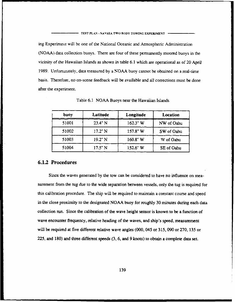
TEST PLA N - NAVSEA TWO BODY TOWING EXPERIMENT
ing Experiment will be one of the National Oceanic and Atmospheric Administration
(NOAA) data collection buoys. There are four of these permanently moored buoys in the
vicinity of the Hawaiian Islands as shown in table 6.1 which are operational as of 20 April
1989. Unfortunately, data measured by a NOAA buoy cannot be obtained on a real-time
basis. Therefore, no on-scene feedback will be available and all corrections must be done
after the experiment.
Table 6.1 NOAA Buoys near the Hawaiian Islands
buoy Latitude Longitude Location
51001 23.4" N 162.3" W NW of Oahu
51002 17.20 N 157.8* W SW of Oahu
51003 19.2" N 160.8" W W of Oahu
51004 17.5" N 152.6" W SE of Oahu
6.1.2 Procedures
Since the waves generated by the tow can be considered to have no influence on mea-
surement from the tug due to the wide separation between vessels, only the tug is required for
this calibration procedure. The ship will be required to maintain a constant course and speed
in the close proximity to the designated NOAA buoy for roughly 30 minutes during each data
collection run. Since the calibration of the wave height sensor is known to be a function of
wave encounter frequency, relative heading of the waves, and ship's speed, measurement
will be required at five different relative wave angles (000, 045 or 315, 090 or 270, 135 or
225, and 180) and three different speeds (3, 6, and 9 knots) to obtain a complete data set.
139

TEST PLAN- NAVSEA TWO BODY TOWING EXPERIMENT
Primary data collection will be performed using instrumentation installed specifically
for this experiment. However, to afford a measure of redundancy, it is requested the SAL-
VOR's navigation team assist in the data collection effort. Table 6.3 presents a summary of
the data to be recorded during this calibration procedure including the frequency of
measurement and responsibility for data collection. Enclosure (2) is provided to assist in
manual data collection.
Table 6.3 Required Data Collection for Wave Height Sensor Calibration
PARAMETER INSTRUMENT FREQUENCY COLLECTED BY
Wave Height portable sensor 2 Hz MIT
Wind Speed portable sensor 2 Hz MITship's sensor 5 min ARS 52
Wind Direction portable sensor 2 Hz MITship's sensor 5 main ARS 52
Speed portable LORAN C 1 min MITship's pit log 1 min ARS 52
Position navigation fix 10 min + ARS 52begin & end
6.2 Flux Gate Compass
6.2.1 Overview
Since a magnetic compass, whether mechanical or electronic, is sensitive to magnetic
fields, any magnetic disturbance near the compass will deflect it from the proper reading.
140

TEST PLAN - NAVSEA TWO BODY TOWING EXPERIMENT
Both the permanent and induced magnetism of the ship will influence compass readings and
therefore provisions must be made to compensate for these forces. Preliminary compass
adjustments can be accomplished pierside to minimize the effects of the inherent magnetic
properties of steel and hard iron used in construction of the ship. However, since the induced
magnetic signature of the ship is dynamic in nature and varies depending on the ship's loca-
tion and orientation with respect to the magnetic poles, final compass corrections can only be
performed at sea.
6.2.2 Procedure
Magnetic compasses are normally calibrated by comparison to a compass of known
deviation through a standard procedure known as "swinging the ship." This involves steam-
ing the ship on various magnetic headings and comparing the compass readings to a refer-
ence compass. For the Two Body Towing Experiment, calibration of the flux gate
compasses will be accomplished by steaming the ship in known reference directions
(typically the eight cardinal and intercardinal headings) and comparing their measured head-
ing with that of the ship's installed magnetic compass. Knowing the deviation of the ship's
magnetic compass, the deviation of the flux gate compasses can be computed. This
procedure can be done in conjunction with the wave height sensor calibration described
above.
The HECTOR will also have an installed flux gate compass which must be calibrated.
However, since her installed magnetic compass will not be operational, the SALVOR's mag-
netic compass must be used as the reference compass for calibration. To use the magnetic
compass of one ship to determine the deviation of a compasses on another ship will require
intricate ship handling; something that salvage ship drivers have proven experience. The
141

TEST PL N - NAVSEA TWO BODY TOWING EXPERMINT
HECTOR's flux gate compass will be calibrated as the two ships are proceeding out of port
to conduct the data collection phase. This will require the tug to maneuver into a position
such that the centerline of both the tug and tow are aligned, as visually verified from the tug's
pelorus, on each courses used in the tug's flux gate compass correction. At the moment that
the tow vessels are aligned, simultaneous recordings of the headings from both flux gate
compasses and the tug's magnetic compass will be taken. The reading from the tow will be
obtained via telemetry on a real-time basis. Although this will only be a "pseudo" calibration
procedure, it is considered accurate enough for purposes of this experiment since we are
mainly interested in the time-varying changes in the headings of both vessels while towing.
142

II~cj,~ 4.)
4)
~-o -4.) -Z I-.
C - - - - - - - -o -I-
4.)
2
4.)4.) =
4.)4)r~v~
o ------------
~-u~ Q 0z --oI- U
~) -
0
-. - 4.)0 ~
o___ C.)
CU 0ats -
0 ~4.)
-
00- .-.- - -S ~ -~ -~ - -S ~ '. .
0E~
U--Uz
- = - - --- mm-rn
E4.)
- - - - - - --- - rn - rn