Planning for Disruptions in Supply Chain Networks · It is easy to view supply uncertainty and...

INFORMS—New Orleans 2005 c© 2005 INFORMS | isbn 0000-0000doi 10.1287/educ.1053.0000

Planning for Disruptions in Supply Chain

Networks

Lawrence V. SnyderLehigh University, [email protected]

Paola M. ScaparraUniversity of Kent, [email protected]

Mark S. DaskinNorthwestern University, [email protected]

Richard L. ChurchUniversity of California, Santa Barbara, [email protected]

Abstract Recent events have highlighted the need for planners to consider the risk of disruptionswhen designing supply chain networks. Supply chain disruptions have a number ofcauses and may take a number of forms. Once a disruption occurs, there is very littlerecourse regarding supply chain infrastructure since these strategic decisions cannotbe changed quickly. Therefore, it is critical to account for disruptions during the designof supply chain networks so that they perform well even after a disruption. Indeed,these systems can often be made substantially more reliable with only small additionalinvestments in infrastructure.

Planners have a range of options available to them in designing resilient supply chainnetworks, and their choice of approaches will depend on the financial resources avail-able, the decision maker’s risk preference, the type of network under consideration,and other factors. In this tutorial, we present a broad range of models for designingsupply chains that are resilient to disruptions. We first categorize these models bythe status of the existing network: a network may be designed from scratch, or anexisting network may be modified to prevent disruptions at some facilities. We nextdivide each of these categories based on the underlying optimization model (facilitylocation or network design) and the risk measure (expected cost or worst-case cost).

Keywords facility location, network design, disruptions

1. Introduction

1.1. Motivation

Every supply chain faces disruptions of various sorts. Recent examples of major disruptionsare easy to bring to mind: Hurricanes Katrina and Rita in 2005 on the U.S. Gulf Coastcrippled the nation’s oil refining capacity [65], destroyed large inventories of coffee andlumber [3, 71], and forced the rerouting of bananas and other fresh produce [3]. A strike attwo General Motors parts plants in 1998 led to the shutdowns of 26 assembly plants andultimately prevented the company from building over 500,000 vehicles and led to a $809million quarterly loss [13, 85, 86]. An eight-minute fire at a Philips semiconductor plant in2001 brought one customer, Ericsson, to a virtual standstill while another, Nokia, weatheredthe disruption [55]. Moreover, smaller-scale disruptions occur much more frequently. Forexample, Wal-Mart’s Emergency Operations Center receives a call virtually every day froma store or other facility with some sort of crisis [57].

1

2 INFORMS—New Orleans 2005, c© 2005 INFORMS

There is evidence that superior contingency planning can significantly mitigate the effect ofa disruption. For example, Home Depot’s policy of planning for various types of disruptionsbased on geography helped it get 23 of its 33 stores within Katrina’s impact zone open afterone day and 29 after one week [35], and Wal-Mart’s stock pre-positioning helped make ita model for post-hurricane recovery [57]. Similarly, Nokia weathered the 2001 Phillips firethrough superior planning and quick response, allowing it ultimately to capture a substantialportion of Ericsson’s market share [55].

Recent books and articles in the business and popular press have pointed out the vul-nerability of today’s supply chains to disruptions and the need for a systematic analysis ofsupply chain vulnerability, security, and resiliency [33, 49, 60, 73, 81]. One common themeamong these references is that the tightly optimized, just-in-time, lean supply chain practiceschampioned by practitioners and OR researchers in recent decades increase the vulnerabil-ity of these systems. Many have argued that supply chains should have more redundancyor slack to provide a buffer against various sorts of uncertainty. Nevertheless, companieshave historically been reluctant to invest much in additional supply chain infrastructure orinventory, despite the large payoff that such investments can have if a disruption occurs.

We argue that decision makers should take supply uncertainty (of which disruptions areone variety) into account during all phases of supply chain planning, just as they accountfor demand uncertainty. This is most critical during strategic planning since these decisionscannot easily be modified. When a disruption strikes, there is very little recourse for strategicdecisions like facility location and network design. (By contrast, firms can often adjustinventory levels, routing plans, production schedules, and other tactical and operationaldecisions in real time in response to unexpected events.)

It is easy to view supply uncertainty and demand uncertainty as two sides of the samecoin. For example, a toy manufacturer may view stockouts of a hot new toy as a result ofdemand uncertainty, but to a toy store the stockouts look like a supply-uncertainty issue.Many of the techniques that firms use to mitigate demand uncertainty—safety stock, supplierredundancy, forecast refinements—are also applicable in the case of supply uncertainty.However, it is dangerous to assume that supply uncertainty is a special case of demanduncertainty or that it can be ignored by decision makers, because much of the conventionalwisdom gained from studying demand uncertainty does not hold under supply uncertainty.For example, under demand uncertainty, it may be optimal for a firm to operate fewer DCsbecause of the risk pooling effect and economies of scale in ordering [27], while under supplyuncertainty it may be optimal to operate more, smaller DCs so that a disruption to one ofthem has a smaller impact. Snyder and Shen [92] discuss this and other differences betweenthe two forms of uncertainty.

In this tutorial, we discuss models for designing supply chain networks that are resilientto disruptions. The objective is to design the supply chain infrastructure so that it operatesefficiently (i.e., at low cost) both normally and when a disruption occurs. We discuss mod-els for facility location and network design. Additionally, we analyze fortification modelswhich can be used to improve the reliability of infrastructure systems which are already inplace and for which a complete reconfiguration would be cost prohibitive. The objective offortification models is to identify optimal strategies for allocating limited resources amongpossible mitigation investments.

1.2. Taxonomy and Tutorial Outline

We classify models for reliable supply chain design along three axes:

(1) Design vs. fortification. Is the model intended to create a reliable network assumingthat no network is currently in place, or to fortify an existing network to make it morereliable?

INFORMS—New Orleans 2005, c© 2005 INFORMS 3

(2) Underlying model. Reliability models generally have some classical model as theirfoundation. In this tutorial, we consider models that are based on facility location andnetwork design models.

(3) Risk measure. As in the case of demand uncertainty, models with supply uncertaintyneed some measure for evaluating risk. Examples include expected cost and minimaxcost.

This tutorial is structured according to this taxonomy. Section 3 discusses design models,while Section 4 discusses fortification models, with subsections in each to divide the modelsaccording to the remaining two axes. These sections are preceded by a review of the relatedliterature in Section 2 and followed by conclusions in Section 5.

2. Literature Review

We discuss the literature that is directly related to reliable supply chain network designthroughout this tutorial. In this section, we briefly discuss several streams of research thatare indirectly related. For more detailed reviews of facility location models under uncertainty,the reader is referred to [28, 67, 87]. An excellent overview of stochastic programming theoryin general is provided in [43].Network Reliability Theory The concept of supply chain reliability is related to net-work reliability theory [22, 83, 84], which is concerned with calculating or maximizing theprobability that a graph remains connected after random failures due to congestion, disrup-tions, or blockages. Typically this literature considers disruptions to the links of a network,but some papers consider node failures [32], and in some cases the two are equivalent.Given the difficulty in computing the reliability of a given network, the goal is often tofind the minimum-cost network with some desirable property like 2-connectivity [63, 64],k-connectivity [11, 39], or special ring structures [34]. The key diference between networkreliability models and the models we discuss in this tutorial is that network reliability mod-els are primarily concerned with connectivity; they consider the cost of constructing thenetwork but not the cost that results from a disruption, whereas our models consider bothtypes of costs and generally assume connectivity after a disruption.Vector-Assignment Problems Weaver and Church [101] introduce the vector-

assignment P -median problem (VAPMP), in which each customer is assigned to severalopen facilities according to an exogenously determined frequency. For example, a customermight receive 75% of its demand from its nearest facility, 20% from its second-nearest, and5% from its third-nearest. This is similar to the assignment strategy used in many of themodels below, but in our models the percentages are determined endogenously based ondisruptions rather than given as inputs to the model. A vector-assignment model based onthe uncapacitated fixed-charge location problem (UFLP) is presented by [70].Multiple, Excess, and Backup Coverage Models The maximum covering problem[19] locates a fixed number of facilities to maximize the demands located within some radiusof an open facility. It implicitly assumes that the facilities (e.g., fire stations, ambulances)are always available. Several subsequent papers have considered the congestion at facilitieswhen multiple calls are received at the same time. The maximum expected covering locationmodel (MEXCLM) [25, 26] maximizes the expected coverage given a constant, systemwideprobability that a server is busy at any given time. The constant-busy-probability assump-tion is relaxed in the maximum availability location problem (MALP) [72]. A related streamof research explicitly considers the queueing process at the locations; these “hypercube”models are interesting as descriptive models but are generally too complex to embed intoan optimization framework [10, 53, 54]. See [24, 7] for a review of expected and backupcoverage models. The primary differences between these models and the models we discussin this tutorial are (1) the objective function (coverage vs. cost) and (2) the reason for aserver’s unavailability (congestion vs. disruptions).


Inventory Models with Supply Disruptions There is a stream of research in theinventory literature that considers supply disruptions in the context of classical inventorymodels such as the EOQ [68, 5, 88], (Q,R) [40, 69, 61, 62], and (s,S) [1] models. More recentmodels examine a range of strategies for mitigating disruptions, including dual sourcing [97],demand management [98], supplier reliability forecasting [96, 99], and product-mix flexibility[95]. Few models consider disruptions in multi-echelon supply chain or inventory systems;exceptions include [50, 92].Process Flexibility There are at least five strategies that can be employed in the face ofuncertain demands: expanding capacity, holding reserve inventory, improving the demandforecasts, introducing product commonality to delay the need for specialization, and addingflexibility to production plants. A complete review of each of these strategies is beyond thescope of this tutorial. Many of these strategies are fairly straightforward. Process flexibility,on the other hand, warrants a brief discussion. Jordan and Graves [48] compare the expectedlost sales that result from using a set of fully flexible plants, in which each plant couldproduce each product, to a configuration in which each plant produces only two productsand the products are chained in such a way that plant A produces products 1 and 2, plantB produces products 2 and 3, and so on, with the last plant producing the final productas well as product 1. They refer to this latter configuration as a 1-chain. They find that a1-chain provides nearly all of the benefits of total flexibility when measured by the expectednumber of lost sales. Based on this, they recommend that flexibility be added to create fewer,longer chains of products and plants. Bish et al. [12] study capacity allocation schemes forsuch chains (e.g., allocate capacity to the nearest demands, to the highest-margin demands,or to a plant’s primary product). They find that if the capacity is either very small orvery large relative to the expected demand, the gains from managing flexible capacity areoutweighed by the need for additional component inventory at the plants and the costs oforder variability at suppliers. They then provide guidelines for the use of one allocationpolicy relative to others based on the costs of component inventory, component lead times,and profit margins. Graves and Tomlin [38] extend the Jordan and Graves results to multi-stage systems. They contrast the configuration loss with the configuration inefficiency. Theformer measures the difference between the shortfall with total flexibility and the shortfallwith a particular configuration of flexible plants. The configuration inefficiency measures theeffect of the interaction between stages in causing the shortfall for a particular configuration.They show that this, in turn, is caused by two phenomena: floating bottlenecks and stage-spanning bottlenecks. Stage-spanning bottlenecks can arise even if demand is deterministic,as a result of misallocations of capacity across the various stages of the supply chain. Beachet al. [4] and de Toni and Tonchia [29] provide more detailed reviews of the manufacturingflexibility literature.Location of Protection Devices A number of papers in the location literature haveaddressed the problem of finding the optimal location of protection devices to reduce theimpact of possible disruptions to infrastructure systems. For example, Carr et al. [16]present a model for optimizing the placement of sensors in water supply networks to detectmaliciously-injected contaminants. James and Salhi [46] investigate the problem of plac-ing protection devices in electrical supply networks to reduce the amount of outage time.Flow-interception models [6] have also been used to locate protection facilities. For example,[44] and [37] use flow-interception models to locate inspection stations so as to maximizehazard avoidance and risk reduction in transportation networks. The protection models dis-cussed in this chapter differ from those models in that they do not seek for the optimalplacement of physical protection devices or facilities. Rather they aim at identifying themost critical system components to harden or protect with limited protection resources (forexample through structural retrofit, fire safety, increased surveillance, vehicle barriers, andmonitoring systems).


3. Design Models

3.1. Introduction

In this section we discuss design models for reliable facility location and network design.These models, like most facility location models, assume that no facilities currently exist;they aim to choose a set of facility locations that perform well even if disruptions occur. It isalso straightforward to modify these models to account for facilities that may already exist(e.g., by setting the fixed cost of those facilities to 0 or adding a constraint that requiresthem to be open). In contrast, the fortification models discussed in Section 4 assume thatall facility sites have been chosen and attempt to decide which facilities to fortify (pro-tect against disruptions). One could conceivably formulate an integrated design/fortificationmodel whose objective would be to locate facilities and to identify a subset of those facil-ities to fortify against attacks. Formulation of such a model is a relatively straightforwardextension of the models we present below, though its solution would be considerably moredifficult as it would result in (at least) a tri-level optimization problem.

Most models for both classical and reliable facility location are design models, as “forti-fication” is a relatively new concept in the facility location literature. In the sub-sectionsthat follow, we introduce several design models, classified first according to the underlyingmodel (facility location or network design) and then according to risk measure (expected orworst-case cost).

3.2. Facility Location Models

3.2.1. Expected Cost Models In this section, we define the reliability fixed-chargelocation problem (RFLP; [89]), which is based on the classical uncapacitated fixed-chargelocation problem (UFLP; [2]). There is a fixed set I of customer locations and a set J ofpotential facility locations. Each customer i∈ I has an annual demand of hi units, and eachunit shipped from facility j ∈ J to customer i ∈ I incurs a transportation cost of dij . (Wewill occasionally refer to dij as the “distance” between j and i, and use this notion to refer to“closer” or “farther” facilities.) Each facility site has an annual fixed cost fj that is incurredif the facility is opened. Any open facility may serve any customer (that is, there are noconnectivity restrictions), and facilities have unlimited capacity. There is a single product.

Each open facility may fail (be disrupted) with a fixed probability q. (Note that the failureprobability q is the same at every facility. This assumption allows a compact description ofthe expected transportation cost. Below, we relax this assumption and instead formulate ascenario-based model that requires more decision variables but is more flexible.) Failures areindependent, and multiple facilities may fail simultaneously. When a facility fails, it cannotprovide any product, and the customers assigned to it must be re-assigned to non-disruptedfacility.

If customer i is not served by any facility, the firm incurs a penalty cost of θi per unitof demand. This penalty may represent a lost-sales cost or the cost of finding an alternatesource for the product. It is incurred if all open facilities have failed, or if it is too expensiveto serve a customer from its nearest functional facility. To model this, we augment the facilityset J to include a dummy “emergency facility,” called u, that has no fixed cost (fu = 0)and never fails. The transportation cost from u to i is diu ≡ θi. Assigning a customer to theemergency facility is equivalent to not assigning it at all.

The RFLP uses two sets of decision variables:

Xj =

{

1, if facility j is opened,

0, otherwise

Yijr =

{

1, if customer i is assigned to facility j at level r,

0, otherwise


A “level-r” assignment is one for which there are r closer open facilities. For example,suppose that the three closest open facilities to customer i are facilities 2, 5, and 8, inthat order. Then facility 2 is i’s level-0 facility, 5 is its level-1 facility, and 8 is its level-2facility. Level-0 assignments are to “primary” facilities that serve the customer under normalcircumstances, while level-r assignments (r > 0) are to “backup” facilities that serve it ifall closer facilities have failed. A customer must be assigned to some facility at each level r

unless it is assigned to the emergency facility at some level s ≤ r. Since we don’t know inadvance how many facilities will be open, we extend the index r from 0 through |J |−1, butYijr will equal 0 for r greater than or equal to the number of open facilities.

The objective of the RFLP is to choose facility locations and customer assignments tominimize the fixed cost plus the expected transportation cost and lost-sales penalty. Weformulate it as an integer programming problem as follows:

(RFLP) minimize∑

j∈J

fjXj +∑

i∈I

|J|−1∑

r=0

∑

j∈J\{u}

hidijqr(1− q)Yijr + hidiuqrYius

(1)

subject to∑

j∈J

Yijr +

r−1∑

s=0

Yiur = 1 ∀i∈ I, r = 0, . . . , |J | − 1 (2)

Yijr ≤Xj ∀i∈ I, j ∈ J, r = 0, . . . , |J | − 1 (3)|J|−1∑

r=0

Yijr ≤ 1 ∀i∈ I, j ∈ J (4)

Xj ∈ {0,1} ∀j ∈ J (5)Yijr ∈ {0,1} ∀i∈ I, j ∈ J, r = 0, . . . , |J | − 1 (6)

The objective function (1) minimizes the sum of the fixed cost and the expected trans-portation and lost-sales costs. The second term reflects the fact that if customer i is assignedto facility j at level r, it will actually be served by j if all r closer facilities have failed (whichhappens with probability qr) and if j itself has not failed (which happens with probability1− q). Note that we can compute this expected cost knowing only the number of facilitiesthat are closer to i than j is but not which facilities those are. This is a result of our assump-tion that every facility has the same failure probability. If, instead, customer i is assignedto the emergency facility at level r, then it incurs the lost-sales cost diu ≡ θi if its r closestfacilities have failed (which happens with probability qr).

Constraints (2) require each customer i to be assigned to some facility at each level r,unless i has been assigned to the emergency facility at level s < r. Constraints (3) prevent anassignment to a facility that has not been opened, and constraints (4) prohibit a customerfrom being assigned to the same facility at more than one level. Constraints (5) and (6)require the decision variables to be binary. However, constraints (6) can be relaxed to non-negativity constraints since single-sourcing is optimal in this problem, as it is in the UFLP.

Note that we do not explicitly enforce the definition of “level-r assignment” in this for-mulation; that is, we do not require Yijr = 1 only if there are exactly r closer open facilities.Nevertheless, in any optimal solution, this definition will be satisfied since it is optimal toassign customers to facilities by levels in increasing order of distance. This is true sincethe objective function weights decrease for larger values of r, so it is advantageous to usefacilities with smaller dij at smaller assignment levels. A slight variation of this result isproven rigorously in [89].

Snyder and Daskin [89] present a slightly more general version of this model in whichsome of the facilities may be designated as “non-failable.” If a customer is assigned to a non-failable facility at level r, it does not need to be assigned at any higher level. In addition, [89]considers a multi-objective model that minimizes the weighted sum of two objectives, one of


which corresponds to the UFLP cost (fixed cost plus level-0 transportation costs) while theother represents the expected transportation cost (accounting for failures). By varying theweights on the objectives, [89] generate a tradeoff curve and use this to demonstrate that theRFLP can produce solutions that are much more reliable than the classical UFLP solutionbut only slightly more expensive by the UFLP objective. This suggests that reliability canbe “bought” relatively cheaply. Finally, [89] also consider a related model that is based onthe P -median problem [41, 42] rather than the UFLP. They solve all of these models usingLagrangian relaxation.

In general, the optimal solution to the RFLP uses more facilities than that of the UFLP.This tendency toward diversification occurs so that any given disruption affects a smallerportion of the system. It may be viewed as a sort of “reverse risk-pooling effect” in which it isadvantageous to spread the risk of supply uncertainty across multiple facilities (encouragingdecentralization). This is in contrast to the classical risk-pooling effect, which encouragescentralization to pool the risk of demand uncertainty.

Berman, Krass, and Menezes [8] consider a model similar to (RFLP), based on the P -median problem rather than the UFLP. They allow different facilities to have different failureprobabilities, but the resulting model is highly nonlinear and in general must be solvedheuristically. They prove that the Hakimi property applies if co-location is allowed. (TheHakimi property says that optimal locations exist at the nodes of a network, even if facilitiesare allowed on the links.) In [9], the same authors present a variant of this model in whichcustomers do not know which facilities are disrupted before visiting them and must traversea path from one facility to the next until an operational facility is found. For example, acustomer might walk to the nearest ATM, find it out of order, and then walk to the ATMthat is nearest to the current location. They investigate the spatial characteristics of theoptimal solution and discuss the value of reliability information.

An earlier attempt at addressing reliability issues in P -median problems is discussed in[31], which examines the problem of locating P unreliable facilities in the plane so as tominimize expected travel distances between customers and facilities. As in the RFLP, theunreliable P -median problem in [31] is defined by introducing a probability that a facilitybecomes inactive but does not require the failures to be independent events. The problem issolved through a heuristic procedure. A more sophisticated method to solve the unreliableP -median problem was subsequently proposed in [56]. In [31], the authors also present theunreliable (P,Q)-center problem where P facilities must be located while taking into accountthat Q of them may become unavailable simultaneously. The objective is to minimize themaximal distance between demand points and their closest facilities.

The formulation given above for (RFLP) captures the expected transportation cost with-out using explicit scenarios to describe the uncertain events (disruptions). An alternateapproach is to model the problem as a two-stage stochastic programming problem in whichthe location decisions are first-stage decisions and the assignment decisions are made in thesecond stage, after the random disruptions have occurred. This approach can result in amuch larger IP model since there are 2|J| possible failure scenarios and each requires itsown assignment variables. That is, in the formulation above we have |J | Y variables foreach i, j (indexed Yijr , r = 0, . . . , |J | − 1), while in the scenario-based formulation we have2|J| variables for each i, j. However, formulations built using this approach can be solvedusing standard stochastic programming methods. They can also be adapted more readily tohandle side constraints and other variations.

For example, suppose facility j can serve at most bj units of demand at any given time.These capacity constraints must be satisfied both by “primary” assignments and by re-assignments that occur after disruptions. Let S be the set of failure scenarios such thatajs = 1 if facility j fails in scenario s, and let qs be the probability that scenario s occurs.Finally, let Yijs equal 1 if customer i is assigned to facility j in scenario s and 0 otherwise.The capacitated RFLP can be formulated using the scenario-based approach as follows:


(CRFLP) minimize∑

j∈J

fjXj +∑

s∈S

qs

∑

i∈I

∑

j∈J

hidijYijs (7)

subject to∑

j∈J

Yijs = 1 ∀i∈ I, s∈ S (8)

Yijs ≤Xj ∀i∈ I, j ∈ J, s∈ S (9)∑

i∈I

hiYijs ≤ (1− ajs)bj ∀j ∈ J, s∈ S (10)

Xj ∈ {0,1} ∀j ∈ J (11)Yijs ∈ {0,1} ∀i∈ I, j ∈ J, s∈ S (12)

Note that the set J in this formulation still includes the emergency facility u. The objectivefunction (7) computes the sum of the fixed cost plus the expected transportation cost,taken across all scenarios. Constraints (8) require every customer to be assigned to somefacility (possibly u) in every scenario, and constraints (9) require this facility to be opened.Constraints (10) prevent the total demand assigned to facility j in scenario s from exceedingj’s capacity and prevent any demand from being assigned if the facility has failed in scenarios. Constraints (11) and (12) are integrality constraints. Integrality can be relaxed to non-negativity for the Y variables, if single-sourcing is not required. (Single-sourcing is no longeroptimal because of the capacity constraints.)

(CRFLP) can be modified easily without destroying its structure, in a way that (RFLP)cannot. For example, if the capacity during a disruption is reduced but not eliminated, wecan simply re-define ajs to be the proportion of the total capacity that is affected by thedisruption. We can also easily allow the demands and transportation costs to be scenariodependent.

The disadvantage, of course, is that the number of scenarios grows exponentially with|J |. If |J | is reasonably large, enumerating all of the scenarios is impractical. In this case,one generally must use sampling techniques such as sample average approximation (SAA;[51, 59, 80]), in which the optimization problem is solved using a subset of the scenariossampled using Monte Carlo simulation. By solving a series of such problems, one can developbounds on the optimal objective value and the objective value of a given solution. Ulkerand Snyder [100] present a method for solving (CRFLP) that uses Lagrangian relaxationembedded in an SAA scheme.

An ongoing research project has focused on extending the models discussed in this sectionto account for inventory costs when making facility location decisions. Jeon, Snyder, andShen [47] consider facility failures in a location–inventory context that is similar to themodels propsed recently by [27, 82], which account for the cost of cycle and safety stock.The optimal number of facilities in the models by [27, 82] is smaller than those in the UFLPdue to economies of scale in ordering and the risk-pooling effect. Conversely, the optimalnumber of facilities is larger in the RFLP than in the UFLP to reduce the impact of anysingle disruption. The location–inventory model with disruptions proposed by [47] finds abalance between these two competing tendencies.

3.2.2. Worst-Case Cost Models Models that minimize the expected cost, as in Sec-tion 3.2.1, take a risk-neutral approach to decision-making under uncertainty. Risk-aversedecision makers may be more inclined to minimize the worst-case cost, taken across all sce-narios. Of course, in this context it does not make sense to consider all possible scenarios,since otherwise the worst-case scenario is always the one in which all facilities fail. Instead,we might consider all scenarios in which, say, at most three facilities fail, or all scenarioswith probability at least 0.01, or some other set of scenarios identified by managers as worth


planning against. In general, the number of scenarios in such a problem is smaller than inthe expected-cost problem since scenarios that are clearly less costly than other scenarioscan be omitted from consideration. For example, if we wish to consider scenarios in whichat most three facilities fail, we can ignore scenarios in which two or fewer fail.

To formulate the minimax-cost RFLP, we introduce a single additional decision variableU , which equals the maximum cost.

(MMRFLP) minimize U (13)

subject to∑

j∈J

fjXj +∑

i∈I

∑

j∈J

hidijYijs ≤U ∀s∈ S (14)

∑

j∈J

Yijs = 1 ∀i∈ I, s∈ S (15)

Yijs ≤Xj ∀i∈ I, j ∈ J, s∈ S (16)Xj ∈ {0,1} ∀j ∈ J (17)

Yijs ∈ {0,1} ∀i∈ I, j ∈ J, s∈ S (18)

In this formulation we omit the capacity constraints (10), but they can be included withoutdifficulty. Unfortunately, minimax models tend to be much more difficult to solve exactly,either with general-purpose IP solvers or with customized algorithms. This is true for clas-sical problems as well as for (MMRFLP).

The regret of a solution under a given scenario is the relative or absolute difference betweenthe cost of the solution under that scenario and the optimal cost under that scenario. One canmodify (MMRFLP) easily to minimize the maximum regret across all scenarios by replacingthe right-hand side of (14) with U +zs (for absolute regret) or zs(1+U) (for relative regret).Here, zs is the optimal cost in scenario s, which must be determined exogenously for eachscenario and provided as an input to the model.

Minimax-regret problems may require more scenarios than their minimax-cost counter-parts since it is not obvious a priori which scenarios will produce the maximum regret. Onthe other hand, they tend to result in a less pessimistic solution than minimax-cost mod-els do. Snyder and Daskin [91] discuss minimax-cost and minimax-regret models in furtherdetail and provide computational results.

One common objection to minimax models is that they are overly conservative sincethe resulting solution plans against a single scenario, which may be unlikely even if it isdisastrous. In contrast, expected-cost models like (CRFLP) produce solutions that performwell in the long run but may perform poorly in some scenarios. Snyder and Daskin [91]introduce a model that avoids both of these problems by minimizing the expected cost (7)subject to a constraint on the maximum cost that can occur in any scenario (in effect,treating U as a constant in (14)). An optimal solution to this model is guaranteed to performwell in the long run (due to the objective function) but is also guaranteed not to be disastrousin any given scenario. This approach is closely related to the concept of p-robustness inrobust optimization problems [52, 90]. One computational disadvantage is that, unlike theother models we have discussed, it can be difficult (even NP-hard) to find a feasible solutionor to determine whether a given instance is feasible. See [91] for more details on this model,and for a discussion of reliable facility location under a variety of other risk measures.

Church et al. [18] use a somewhat different approach to model worst-case cost designproblems, the rationale being that the assumption of independent facility failures underlyingthe previous models does not hold in all application settings. This is particularly true whenmodeling intentional disruptions. As an example, a union or a terrorist could decide tostrike those facilities in which the greatest combined harm (as measured by increased costs,disrupted service, etc) is achieved. In order to design supply systems able to withstandintentional harms by intelligent perpetrators, [18] proposes the resilient P -median problem.


This model identifies the best location of P facilities so that the system works as well aspossible (in terms of weighted distances) in the event of a maximally disruptive strike.The model is formulated as a bilevel optimization model, where the upper-level problemof optimally locating P facilities embeds a lower-level optimization problem which is usedto generate the weighted distance after a worst-case loss of R of these located P facilities.This bilevel programming approach has been widely used to assess worst-case scenariosand identify critical components in existent systems and will be discussed in more depthin Section 4.2.2. Church et al. [18] demonstrate that optimal P -median configurations canbe rendered very inefficient in terms of worst-case loss, even for small values of R. Theyalso demonstrate that resilient design configurations can be near optimal in efficiency ascompared to the optimal P -median configurations, but at the same time maintain highlevels of efficiency after worst-case loss. A form of the resilient design problem has also beendeveloped for a coverage-type service system [66]. The resilient coverage model finds theoptimal location of a set of facilities to maximize a combination of initial demand coverageand the minimum coverage level following the loss of one or more facilities. There are severalapproaches that one can employ to solve this problem, including the successive use of supervalid inequalities [66], reformulation into a single-level optimization problem when R = 1 orR = 2 [18], or by developing a special search tree. Research is underway to model resilientdesign for capacitated problems.

3.3. Network Design Models

We now turn our attention from reliability models based on facility location problems tothose based on network design models. We have a general network G = (V,A). Each nodei∈ V serves as either a source, sink, or transshipment node. Source nodes are analogous tofacilities in Section 3.2 while sink nodes are analogous to customers. The primary differencebetween network design models and facility location ones is the presence of transshipmentnodes. Product originates at the source nodes and is sent through the network to the sinknodes via transshipment nodes.

Like the facilities in Section 3.2, the non-sink nodes in these models can fail randomly.The objective is to make open/close decisions on the non-sink nodes (first-stage variables)and determine the flows on the arcs in each scenario (second-stage variables) to minimizethe expected or worst-case cost. (Many classical network design problem involve open/closedecisions on arcs, but the two are equivalent through a suitable transformation.)

3.3.1. Expected Cost Each node j ∈ V has a supply bj. For source nodes, bj representsthe available supply and bj > 0; for sink nodes, bj represents the (negative of the) demandand bj < 0; and for transshipment nodes, bj = 0. There is a fixed cost fj to open each non-sink node. Each arc (i, j) has a cost of dij for each unit of flow transported on it and eachnon-sink node j has a capacity kj . The node capacities can be seen as production limitationsfor the supply nodes and processing resource restrictions for the transhipment nodes.

As in Section 3.2.1, we let S be the set of scenarios, and ajs = 1 if node j fails in scenarios. Scenario s occurs with probability qs. To ensure feasibility in each scenario, we augment V

by adding a dummy source node u that makes up any supply shortfall caused by disruptionsand a dummy sink node v that absorbs any excess supply. There is an arc from u to each(non-dummy) sink node; the per-unit cost of this arc is equal to the lost-sales cost for thatsink node (analogous to θi in Section 3.2.1). Similarly, there is an arc from each (non-dummy)source node to v whose cost equals 0. The dummy source node and the dummy sink nodehave infinite supply and demand, respectively.

Let V0 ⊆ V be the set of supply and transhipment nodes, i.e., V0 = {j ∈ V |bj ≥ 0}. Wedefine two sets of decision variables. Xj = 1 if node i is opened and 0 otherwise, for j ∈ V0,and Yijs is the amount of flow sent on arc (i, j) ∈A in scenario s ∈ S. Note that the set A

represents the augmented set of arcs, including the arcs outbound from the dummy source


node and the arcs inbound to the dummy sink node. With this notation, the reliable networkdesign model (RNDP) is formulated as follows:

(RNDP) minimize∑

j∈V0

fjXj +∑

s∈S

qs

∑

(i,j)∈A

dijYijs (19)

subject to∑

(j,i)∈A

Yjis −∑

(i,j)∈A

Yijs = bj ∀j ∈ V \ {u, v}, s∈ S (20)

∑

(j,i)∈A

Yjis ≤ (1− ajs)kjXj ∀j ∈ V0, s∈ S (21)

Xj ∈ {0,1} ∀j ∈ V0 (22)Yijs ≥ 0 ∀(i, j)∈A,s∈ S (23)

The objective function computes the fixed cost and expected flow costs. Constraints (20)are the flow-balance constraints for the non-dummy nodes; they require the net flow fornode j (flow out minus flow in) to equal the node’s deficit bj in each scenario. Constraints(21) enforce the node capacities and prevent any flow emanating from a node j that has notbeen opened (Xj = 0) or has failed (ajs = 1). Taken together with (20), these constraints aresufficient to ensure that flow is also prevented into nodes that are not opened or have failed.Constraints (22) and (23) are integrality and non-negativity constraints, respectively. Notethat in model (19)–(23), no flow restrictions are necessary for the two dummy nodes. Theminimization nature of the objective function guarantees that the demand at each sink nodeis supplied from regular source nodes whenever this is possible. Only if the node disruptionis such to prevent some demand node i from being fully supplied will there be a positiveflow on the link (u, i) at the cost dui = θi. Similarly, only excess supply which cannot reacha sink node will be routed to the dummy sink.

This formulation is similar to the model introduced by [75]. Their model is intended fornetwork design under demand uncertainty, while ours considers supply uncertainty, thoughthe two approaches are quite similar. To avoid enumerating all of the possible scenarios, [75]uses SAA. A similar approach is called for to solve (RNDP) since, as in the scenario-basedmodels in Section 3.2.1, if each node can fail independently, we have 2|V0| scenarios.

A scenario-based model for the design of failure-prone multi-commodity networks is dis-cussed in [36]. However, the model in [36] does not consider the expected costs of routingthe commodities through the network. Rather, it determines the minimum-cost set of arcsto be constructed so that the resulting network continues to support a multi-commodityflow under any of a given set of failure scenarios. Only a restricted set of failure scenariosis considered, where each scenario consists of the concurrent failure of multiple arcs. [36]also discusses several algorithmic implementations of Benders decomposition to solve thisproblem efficiently.

3.3.2. Worst-Case Cost One can modify (RNDP) to minimize the worst-case cost ratherthan the expected cost in a manner analogous to the approach taken in Section 3.2.2:


minimize U (24)

subject to∑

i∈V0

fiXi +∑

(i,j)∈A

dijYijs ≤U ∀s∈ S (25)

(20)− (23)

Similarly, one could minimize the expected cost subject to a constraint on the cost in

any scenario, as proposed above. Bundschuh, Klabjan, and Thurston [15] take a similarapproach in a supply chain network design model (with open/close decisions on arcs). They

assume that suppliers can fail randomly. They consider two performance measures, which

they call reliability and robustness. The reliability of the system is the probability that all

suppliers are operable, while robustness refers to the ability of the supply chain to maintain

a given level of output after a failure. The latter measure is perhaps a more reasonablegoal since adding new suppliers increases the probability that one or more will fail and

hence decreases the system’s “reliability.” They present models for minimizing the fixed

and (non-failure) transportation costs subject to constraints on reliability, robustness, or

both. Their computational results support the claim made by [89, 91] and others that large

improvements in reliability can often be attained with small increases in cost.

4. Fortification Models

4.1. Introduction

Computational studies of the models discussed in the previous sections demonstrate that the

impact of facility disruptions can be mitigated by the initial design of a system. However,redesigning an entire system is not always reasonable given the potentially large expense

involved with relocating facilities, changing suppliers or reconfiguring networked systems.

As an alternative, the reliability of existing infrastructure can be enhanced through efficient

investments in protection and security measures. In light of recent world events, the identifi-

cation of cost-effective protection strategies has been widely perceived as an urgent prioritywhich demands not only greater public policy support [94], but also the development of

structured and analytical approaches [49]. Planning for facility protection, in fact, is an

enormous financial and logistical challenge if one considers the complexity of today’s logis-

tics systems, the interdependencies among critical infrastructures, the variety of threats and

hazards, and the prohibitive costs involved in securing large numbers of facilities. Despitethe acknowledged need for analytical models able to capture these complexities, the study

of mathematical models for allocation of protection resources is still in its infancy. The few

fortification models which have been proposed in the literature are discussed in this section,

together with possible extensions and variations.

4.2. Facility Location Models

Location models which explicitly address the issue of optimizing facility protection assume

the existence of a supply system with P operating facilities. Facilities are susceptible todeliberate sabotage or accidental failures, unless protective measures are taken to prevent

their disruption. Given limited protection resources, the models aim to identify the subset

of facilities to protect in order to minimize efficiency losses due to intentional or accidental

disruptions. Typical measures of efficiency are distance traveled, transportation cost, or

captured demand.


4.2.1. Expected Cost Models In this section, we present the P -median fortificationproblem (PMFP; [76]). This model builds upon the well known P -median problem [41, 42].It assumes that the P facilities in the system have unlimited capacity and that the systemusers receive service from their nearest facility. As in the design model RFLP, each facilitymay fail or be disrupted with a fixed probability q. A disrupted facility becomes inoperable,so that the customers currently served by it must be reassigned to their closest non-disruptedfacility. Limited fortification resources are available to protect Q of the P facilities. A pro-tected facility becomes immune to disruption. PMFP identifies the fortification strategythat minimizes the expected transportation costs.

The model definition builds upon the notation used in the previous sections, with theexception that J now denotes the set of existent, rather than potential, facilities. Addi-tionally, let ik denote the kth closest facility to customer i and let dk

i be the expectedtransportation cost between customer i and its closest operational facility, given that thek − 1 closest facilities to i are not protected and the kth closest facility to i is protected.These expected costs can be calculated as follows.

dki =

k−1∑

j=1

qj−1(1− q)diij+ qk−1diik

(26)

The PMFP uses two sets of decision variables:

Zj =

{

1, if facility j is fortified,

0, otherwise

Wik =

1, if the k− 1 closest facilities to customer i are not protected but the kth

closest facility is,

0, otherwise

Then PMFP can be formulated as the following mixed integer program:

(PMFP) minimize∑

i∈I

P−Q+1∑

k=1

hidki Wik (27)

subject to

P−Q+1∑

k=1

Wik = 1 ∀i∈ I, (28)

Wik ≤Zik∀i∈ I, k = 1, . . . , P −Q + 1 (29)

Wik ≤ 1−Zik−1∀i∈ I, k = 2, . . . , P −Q + 1 (30)

∑

j∈J

Zj = Q (31)

Wik ∈ {0,1} ∀i∈ I, k = 1, . . . , P −Q + 1 (32)Zj ∈ {0,1} ∀j ∈ J (33)

The objective function (27) minimizes the weighted sum of expected transportation costs.Note that the expected costs dk

i and the variables Wik need only be defined for values ofk between 1 and P − Q + 1. In fact, in the worst case, the closest protected facility tocustomer i is its (P − Q + 1)st-closest facility. This occurs if the Q fortified facilities arethe Q furthest facilities from i. If all of the P − Q closest facilities to i fail, customer i

is assigned to its (P − Q + 1)st-closest facility. Assignments to facilities that are furtherthan the (P −Q + 1)st-closest facility will never be made in an optimal solution. For eachcustomer i, constraints (28) force exactly one of the P −Q + 1 closest facilities to i to beits closest protected facility. The combined use of constraints (29) and (30) ensures that the


variable Wik that equals 1 is the one associated with the smallest value of k such that thekth closest facility to i is protected. Constraint (31) specifies that only Q facilities can beprotected. Finally, constraints (32) and (33) represent the integrality requirements of thedecision variables.

The PMFP is an integer programming model and can be solved with general purposemixed-integer programming software. Possible extensions of the model include the caseswhere facilities have different failure probabilities and where fortification only reduces, butdoes not eliminate, the probability of failure. Unfortunately, PMFP cannot be easily adjustedto handle capacity restrictions. As for the design version of the problem, if the systemfacilities have limited capacities, explicit scenarios must be used to model possible disruptionpatterns. The capacitated version of PMFP can be formulated in an analogous way to thescenario-based model CRFLP discussed in Section 3.2.1. Namely:

(CPMFP) minimize∑

s∈S

qs

∑

i∈I

∑

j∈J

hidijYijs (34)

subject to∑

j∈J

Yijs = 1 ∀i∈ I, s∈ S (35)

∑

i∈I

hiYijs ≤ (1− ajs)bj + ajsbjZj ∀j ∈ J, s∈ S (36)

∑

j∈J

Zj = Q (37)

Xj ∈ {0,1} ∀j ∈ J (38)Yijs ∈ {0,1} ∀i∈ I, j ∈ J, s∈ S (39)

CPMFP uses the same parameters ajs and set S as CRFLP to model different scenarios.It also assumes that the set of existent facilities J is augmented with the unlimited-capacityemergency facility u. CPMFP differs from CRFLP only in a few aspects: no decisions mustbe made in terms of facility location, so the fixed cost for locating facilities are not includedin the objective; the capacity constraints (36) must reflect the fact that if a facility j isprotected (Zj = 1), then that facility remains operable (and can supply bj units of demand)even in those scenarios s which assume its failure (ajs = 1). Finally, constraint (37) must beadded to fix the number of possible fortifications.

Note that in both models PMFP and CPMFP, the cardinality constraints (31) and (37)can be replaced by more general resource constraints to handle the problem where eachfacility requires a different amount of protection resources and there is a limit on thetotal resources available for fortification. Alternately, one could incorporate this cost intothe objective function and omit the budget constraint. The difference between these twoapproaches is analogous to that between the P -median problem and the UFLP.

4.2.2. Worst-Case Cost Models When modeling protection efforts, it is crucial totake account for hazards to which a facility may be exposed. It is evident that protectingagainst intentional attacks is fundamentally different from protecting against acts of nature.Whereas nature hits at random and does not adjust its behavior to circumvent securitymeasures, an intelligent adversary may adjust its offensive strategy depending on whichfacilities have been protected, for example by hitting different targets. The expected costmodels discussed in Section 4.2.1 do not take into account the behavior of adversaries andare therefore more suitable to model situations in which natural and accidental failures area major concern. The models in this section have been developed to identify cost-effectiveprotection strategies against malicious attackers.

A natural way of looking at fortification problems involving intelligent adversaries is withinthe framework of a leader-follower or Stackelberg game [93], in which the entity responsible


for coordinating the fortification activity, or defender, is the leader and the attacker, orinterdictor, is the follower. Stackelberg games can be expressed mathematically as bilevelprogramming problems [30]: the upper level problem involves decisions to determine whichfacilities to harden, whereas the lower level problem entails the interdictor’s response ofwhich unprotected facilities to attack to inflict maximum harm. Even if in practice wecannot assume that the attacker is always able to identify the best attacking strategy, theassumption that the interdictor attacks in an optimal way is used as a tool to model worst-case scenarios and estimate worst-case losses in response to any given fortification strategy.

The worst-case cost version of PMFP was formulated as a bilevel program in [79]. Themodel, called the R-interdiction median model with fortification (RIMF), assumes that thesystem defender has resources to protect Q facilities, whereas the interdictor has resourcesto attack R facilities, with Q + R < P . In addition to the fortification variables Zj definedin Section 4.2.1, RIMF uses the following interdiction and assignment variables:

Sj =

{

1, if facility j is interdicted,

0, otherwise

Yij =

{

1, if customer i is assigned to facility j after interdiction,

0, otherwise

Additionally, the formulation uses the set Tij = {k ∈ J |dik > dij} defined for each customeri and facility j. Tij represents the set of existing sites (not including j) that are farther thanj is from demand i. The RIMF can then be stated mathematically as follows:

(RIMF) minimize H(Z) (40)

subject to∑

j∈J

Zj = Q (41)

Zj ∈ {0,1} ∀j ∈ J (42)

where H(Z) = maximize∑

i∈I

∑

j∈J

hidijYij (43)

∑

j∈J

Yij = 1 ∀i∈ I (44)

∑

j∈J

Sj = R (45)

∑

h∈Tij

Yih ≤ Sj ∀i∈ I, j ∈ J (46)

Sj ≤ 1−Zj ∀j ∈ J (47)Sj ∈ {0,1} ∀j ∈ J (48)Yij ∈ {0,1} ∀i∈ I, j ∈ J (49)

In the above bilevel formulation, the leader allocates exactly Q fortification resources(41) to minimize the highest possible level of weighted distances or costs, H , (40) derivingfrom the loss of R of the P facilities. The fact that H represents worst-case losses afterthe interdiction of R facilities is enforced by the follower problem, whose objective involvesmaximizing the weighted distances or service costs (43). In the lower level interdictionproblem (RIM; [21]), constraints (44) state that each demand point must be assigned to afacility after interdiction. Constraint (45) specifies that only R facilities can be interdicted.Constraint (46) maintains that each customer must be assigned to its closest open facilityafter interdiction. More specifically, these constraints state that if a given facility j is notinterdicted (Sj = 0), a customer i cannot be served by a facility which is further than j from


i. Constraints (47) link the upper- and lower-level problems by preventing the interdictionof any protected facility. Finally, constraints (42), (48) and (49) represent the integralityrequirements for the fortification, interdiction and assignment variables, respectively. Notethat the binary restrictions for the Yij variables can be relaxed, as an optimal solution withfractional Yij variables only occurs when there is a distance tie between two non-disruptedclosest facilities to customer i. Such cases, although interesting, do not affect the optimalityof the solution.

Church and Scaparra [20] and Scaparra and Church [78] demonstrate that it is possible toformulate RIMF as a single-level program and discuss two different single-level formulations.However, both formulations require the explicit enumeration of all possible interdictionscenarios and, consequently, their applicability is limited to problem instances of modestsize. A more efficient way of solving RIMF is through the implicit enumeration schemeproposed in [79] and tailored to the bilevel structure of the problem.

A stochastic version of RIMF, in which an attempted attack on a facility is successful onlywith a given probability, can be obtained by replacing the lower-level interdiction model(43)-(49) with the probabilistic R-interdiction median model introduced in [17].

Different variants of the RIMF model, aiming at capturing additional levels of complexity,are currently under investigation. Ongoing studies focus, for example, on the developmentof models and solution approaches for the capacitated version of RIMF.

RIMF assumes that at most R facilities can be attacked. Given the large degree of uncer-tainty characterizing the extent of man-made and terrorist attacks, this assumption shouldbe relaxed to capture additional realism. An extension of RIMF which include random num-bers of possible losses as well as theoretical results to solve this expected loss version tooptimality are currently under development.

Finally, bilevel fortification models similar to RIMF can be developed for protecting facil-ities in supply systems with different service protocols and efficiency measures. For example,in emergency service and supply systems, the effects of disruption may be better measuredin terms of the reduction in operational response capability. In these problem settings, themost disruptive loss of R facilities would be the one causing the maximal drop in userdemand that can be supplied within a given time or distance threshold. This problem canbe modeled by replacing the interdiction model (43)-(49) with the R-interdiction cover-ing problem introduced in [21] and by minimizing, instead of maximizing, the upper-levelobjective function H , which now represents the worst case demand coverage decrease afterinterdiction.

4.3. Network Design Models

The literature dealing with the disruption of existent networked systems has primarilyfocused on the analysis of risk and vulnerabilities through the development of interdictionmodels. Interdiction models have been used by several authors to identify the most criticalcomponents of a system, i.e., those nodes or linkages that, if disabled, cause the greatestdisruption to the flow of services and goods through the network. A variety of models, whichdiffer in terms of objectives and underlying network structures, have been proposed in theinterdiction literature. For example, the effect of interdiction on the maximum flow througha network is studied in [102] and [103]. Israeli and Wood [45] analyze the impact of linkremovals on the shortest path length between nodes. Lim and Smith [58] treat the multi-commodity version of the shortest path problem, with the objective of assessing shipmentrevenue reductions due to arc interdictions. A review of interdiction models is provided in[21].

Whereas interdiction models can help reveal potential weaknesses in a system, they donot explicitly address the issue of optimizing security. Scaparra and Cappanera [77] demon-strate that securing those network components that are identified as critical in an optimalinterdiction solution will not necessarily provide the most cost-effective protection against


disruptions. Optimal interdiction is a function of what is fortified, so it is important to cap-ture this interdependency within a modeling framework. The models detailed in the nextsection explicitly addressed the issue of fortification in networked systems.

4.3.1. Expected Cost In this section, we present the reliable network fortification prob-lem (RNFP), which can be seen as the protection counterpart of the RNDP discussed inSection 3.3.1. The problem is formulated below by using the same notation as in Section 3.3.1and the fortification variables Zj = 1 if node j is fortified, and Zj = 0 otherwise.

(RNFP) minimize∑

s∈S

qs

∑

(i,j)∈A

dijYijs (50)

subject to∑

(j,i)∈A

Yjis −∑

(i,j)∈A

Yijs = bj ∀j ∈ V \ {u, v}, s∈ S (51)

∑

(j,i)∈A

Yjis ≤ (1− ajs)kj + ajskjZj ∀j ∈ V0, s∈ S (52)

∑

j∈J

Zj = Q (53)

Zj ∈ {0,1} ∀j ∈ V0 (54)Yijs ≥ 0 ∀(i, j)∈A,s∈ S (55)

The general structure of the RNFP and the meaning of most of its components are as inthe RNDP. A difference worth noticing is that now the capacity constraints (52) maintainthat each fortified node preserves its original capacity in every failure scenario.

The RNFP can be easily modified to handle the problem in which fortification does notcompletely prevent node failures but only reduces the impact of disruptions. As an example,we can assume that a protected node only retains part of its capacity in case of failureand that the level of capacity which can be secured depends on the amount of protectiveresources invested on that node. To model this variation, we denote by fj the fortificationcost incurred to preserve one unit of capacity at node j and by B the total protectionbudget available. Also, we define the continuous decision variables Tj as the level of capacitywhich is secured at node j (with 0≤ Tj ≤ kj). RNFP can be reformulated by replacing thecapacity constraints (52) and the cardinality constraints (53) with the following two sets ofconstraints:

∑

(j,i)∈A

Yjis ≤ (1− ajs)kj + ajsTj ∀j ∈ V0, s∈ S (56)

and

∑

j∈J

fjTj ≤B (57)

4.3.2. Worst-Case Cost The concept of protection against worst-case losses for networkmodels has been briefly discussed in [14, 74]. The difficulty in addressing this kind of problemis that their mathematical representation requires building tri-level optimization models,to represent fortification, interdiction and network flow decisions. Multi-level optimizationproblems are not amenable to solution by standard mixed integer programming method-ologies and no universal algorithm exists for their solutions. To the best of the authors’knowledge, the first attempt at modeling and solving network problems involving protectionissues was undertaken in [77]. In [77], the authors discuss two different models: in the firstmodel, optimal fortification strategies are identified to thwart as much as possible the action


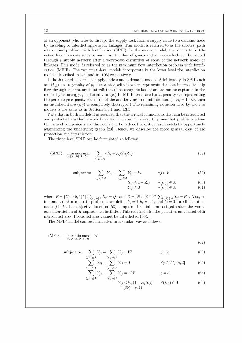
of an opponent who tries to disrupt the supply task from a supply node to a demand nodeby disabling or interdicting network linkages. This model is referred to as the shortest pathinterdiction problem with fortification (SPIF). In the second model, the aim is to fortifynetwork components so as to maximize the flow of goods and services which can be routedthrough a supply network after a worst-case disruption of some of the network nodes orlinkages. This model is referred to as the maximum flow interdiction problem with fortifi-cation (MFIF). The two multi-level models incorporate in the lower level the interdictionmodels described in [45] and in [103] respectively.

In both models, there is a supply node o and a demand node d. Additionally, in SPIF eacharc (i, j) has a penalty of pij associated with it which represents the cost increase to shipflow through it if the arc is interdicted. (The complete loss of an arc can be captured in themodel by choosing pij sufficiently large.) In MFIF, each arc has a penalty rij representingthe percentage capacity reduction of the arc deriving from interdiction. (If rij = 100%, thenan interdicted arc (i, j) is completely destroyed.) The remaining notation used by the twomodels is the same as in Sections 3.3.1 and 4.3.1

Note that in both models it is assumed that the critical components that can be interdictedand protected are the network linkages. However, it is easy to prove that problems wherethe critical components are the nodes can be reduced to critical arc models by opportunelyaugmenting the underlying graph [23]. Hence, we describe the more general case of arcprotection and interdiction.

The three-level SPIF can be formulated as follows:

(SPIF) minZ∈F

maxS∈D

minY

∑

(i,j)∈A

(dij + pijSij)Yij (58)

subject to∑

(j,i)∈A

Yji −∑

(i,j)∈A

Yij = bj ∀j ∈ V (59)

Sij ≤ 1−Zij ∀(i, j)∈A (60)Yij ≥ 0 ∀(i, j)∈A (61)

where F = {Z ∈ {0,1}n|∑

(i,j)∈A Zij = Q} and D = {S ∈ {0,1}n|∑

(i,j)∈A Sij = R}. Also, asin standard shortest path problems, we define bo = 1, bd = −1, and bj = 0 for all the othernodes j in V . The objective function (58) computes the minimum-cost path after the worst-case interdiction of R unprotected facilities. This cost includes the penalties associated withinterdicted arcs. Protected arcs cannot be interdicted (60).

The MFIF model can be formulated in a similar way as follows:

(MFIF) maxz∈F

mins∈D

maxY ≥0

W

(62)

subject to∑

(j,i)∈A

Yji −∑

(i,j)∈A

Yij = W j = o (63)

∑

(j,i)∈A

Yji −∑

(i,j)∈A

Yij = 0 ∀j ∈ V \ {o, d} (64)

∑

(j,i)∈A

Yji −∑

(i,j)∈A

Yij =−W j = d (65)

Yij ≤ kij(1− rijSij) ∀(i, j)∈A (66)(60)− (61)


In MFIF, the objective (62) is to maximize the total flow W through the network after theworst-case interdiction of the capacities of R arcs. Capacity reductions due to interdictionare calculated in (66). Constraints (63)-(65) are standard flow conservation constraints formaximum-flow problems.

The two three-level programs, SPIF and MFIF, can be reduced to bilevel programs bytaking the dual of the inner network flow problems. Scaparra and Cappanera [77] showhow the resulting bilevel problem can be solved efficiently through an implicit enumerationscheme that incorporates network optimization techniques. The authors also show that opti-mal fortification strategies can be identified for relatively large networks (hundreds of nodesand arcs) in reasonable computational time and that significant efficiency gains (in termsof path costs or flow capacities) can be achieved even with modest fortification resources.

Model MFIF can be easily modified to handle multiple sources and multiple destinations.Also, a three-level model can be built along the same lines of SPIF and MFIF for multi-commodity flow problems. For example, by embedding the interdiction model proposed in[58], in the three-level framework, it is possible to identify optimal fortification strategiesfor maximizing the profit that can be obtained by shipping commodities across a network,while taking into account worst-case disruptions.

5. Conclusions

In this tutorial we have attempted to illustrate the wide range of strategic planning modelsavailable for desiging supply chain networks under the threat of disruptions. A planner’schoice of model will depend on a number of factors, including the type of network underconsideration, the status of existing facilities in the network, the firm’s risk preference, andthe resources available for constructing, fortifying, and operating facilities.

We believe that there are several promising avenues for future research in this field. First,the models we discussed in this tutorial tend to be much more difficult to solve than theirreliable-supply counterparts—most have significantly more decision variables, many haveadditional hard constraints, and some have multiple objectives. For these models to beimplemented broadly in practice, better solution methods are required.

The models presented above consider the cost of re-assigning customers or re-routing flowafter a disruption. However, there are other potential repercussions that should be mod-eled. For example, firms may face costs associated with destroyed inventory, reconstructionof disrupted facilities, and customer attrition (if the disruption does not affect the firm’scompetitors). In addition, the competitive environment in which a firm operates may signif-icantly affect the decisions the firm makes with respect to risk mitigation. For many firms,the key objective may be to ensure that their post-disruption situation is no worse thanthat of their competitors. Embedding these objectives in a game theoretic environment isanother important extension.

Finally, most of the existing models for reliable supply chain network design use somevariation of a minimum-cost objective. Such objectives are most applicable for problemsinvolving the distribution of physical goods, primarily in the private sector. But reliabilityis critical in the public sector as well, for the location of emergency services, post-disastersupplies, and so on. In these cases, cost is less important than proximity, suggesting thatcoverage objectives may be warranted. The application of such objectives to reliable facilitylocation and network design problems will enhance the richness, variety, and applicabilityof these models.

References

[1] Antonio Arreola-Risa and Gregory A. DeCroix. Inventory management under random supplydisruptions and partial backorders. Naval Research Logistics, 45:687–703, 1998.

[2] M. L. Balinski. Integer programming: Methods, uses, computation. Management Science,12(3):253–313, 1965.


[3] Alexei Barrionuevo and Claudia H. Deutsch. A distribution system brought to its knees. NewYork Times, page C1, September 1 2005.

[4] R. Beach, A.P. Muhlemann, D.H.R. Price, A. Paterson, and J.A. Sharp. A review of manu-facturing flexibility. European Journal of Operational Research, 122:41–57, 2000.

[5] Emre Berk and Antonio Arreola-Risa. Note on “Future supply uncertainty in EOQ models”.Naval Research Logistics, 41:129–132, 1994.

[6] O. Berman, M. J. Hodgson, and D. Krass. Flow-Interception problems. In Zvi Drezner, editor,Facility Location: A survey of applications and methods, chapter 17, pages 389–426. SpringerSeries in Operations Research, 1995.

[7] Oded Berman and Dimitri Krass. Facility location problems with stochastic demands andcongestion. In Zvi Drezner and H. W. Hamacher, editors, Facility Location: Applications andTheory, pages 331–373. Springer-Verlag, New York, 2002.

[8] Oded Berman, Dmitry Krass, and Mozart B. C. Menezes. Facility reliability issues in networkp-median problems: Strategic centralization and co-location effects. Forthcoming in Opera-tions Research, 2005.

[9] Oded Berman, Dmitry Krass, and Mozart B. C. Menezes. MiniSum with imperfect infor-mation: Trading off quantity for reliability of locations. Working paper, Rotman School ofManagement, University of Toronto, 2005.

[10] Oded Berman, Richard C. Larson, and Samuel S. Chiu. Optimal server location on a networkoperating as an M/G/1 queue. Operations Research, 33(4):746–771, 1985.

[11] D.E. Bienstock, E. F. Brickell, and C.L. Monma. On the structure of minimum-weight k-connected spanning networks. SIAM Journal on Discrete Mathematics, 3:320–329, 1990.

[12] E.K. Bish, A. Muriel, and S. Biller. Managing flexible capacity in a make-to-order environ-ment. Management Science, 51(2):167–180, 2005.

[13] Ken Brack. Ripple effect from GM strike build. Industrial Distribution, 87(8):19, August 1998.

[14] G. G. Brown, W. M. Carlyle, J. Salmeron, and K. Wood. Analyzing the vulnerability ofcritical infrastructure to attach and planning defenses. In H. J. Greenberg, editor, TutORialsin Operations Research, pages 102–123. INFORMS, 2005.

[15] Markus Bundschuh, Diego Klabjan, and Deboarh L. Thurston. Modeling robust and reliablesupply chains. working paper, University of Illinois at Urbana-Champaign, 2003.

[16] R. D. Carr, H. J. Greenberg, W. E. Hart, G. Konjevod, E. Lauer, H. Lin, T. Morrison, andC. A. Phillips. Robust optimization of contaminant sensor placement for community watersystems. Mathematical Programming, 107:337–356, 2005.

[17] R. L. Church and M. P. Scaparra. Analysis of facility systems’reliability when subject to attackor a natural disaster. Reliability and Vulnerability in Critical Infrastructure: A QuantitativeGeographic Perspective, edited by A.T. Murray and T.H. Grubesic, Springer-Verlag, 2006.

[18] R. L. Church, M. P. Scaparra, and J. R. O’Hanley. Optimizing passive protection in facilitysystems. ISOLDE X, Spain, 2005. Working Paper.

[19] Richard Church and Charles ReVelle. The maximal covering location problem. Papers of theRegional Science Association, 32:101–118, 1974.

[20] Richard L. Church and Maria P. Scaparra. Protecting critical assets: The r-interdictionmedian problem with fortification. Working paper 79, Kent Business School, Canterbury,England, February 2005.

[21] Richard L. Church, Maria P. Scaparra, and Richard S. Middleton. Identifying critical infras-tructure: The median and covering facility interdiction problems. Annals of the Associationof American Geographers, 94(3):491–502, 2004.

[22] C. Colbourn. The Combinatorics of Network Reliability. Oxford University Press, New York,1987.

[23] H. W. Corley and H. Chang. Finding the most vital nodes in a flow network. ManagementScience, 21(3):362–364, 1974.

[24] M. S. Daskin, K. Hogan, and C. ReVelle. Integration of multiple, excess, backup, and expectedcovering models. Environment and Planning B, 15(1):15–35, 1988.

[25] Mark S. Daskin. Application of an expected covering model to emergency medical servicesystem design. Decision Sciences, 13:416–439, 1982.

[26] Mark S. Daskin. A maximum expected covering location model: Formulation, properties andheuristic solution. Transportation Science, 17(1):48–70, 1983.


[27] Mark S. Daskin, Collette R. Coullard, and Zuo-Jun Max Shen. An inventory-location model:Formulation, solution algorithm and computational results. Annals of Operations Research,110:83–106, 2002.

[28] Mark S. Daskin, Lawrence V. Snyder, and Rosemary T. Berger. Facility location in supplychain design. In A. Langevin and D. Riopel, editors, Logistics Systems: Design and Operation,chapter 2, pages 39–66. Springer, 2005.

[29] A. de Toni and S. Tonchia. Manufacturing flexibility: A literature review. International Jour-nal of Production Research, 36(6):1587–1617, 1998.

[30] S. Dempe. Foundations of Bilevel Programming. Kluwer Academic Publishers, The Nether-lands, 2002.

[31] Z. Drezner. Heuristic solution methods for two location problems with unreliable facilities.Journal of the Operational Research Society, 38(6):509–514, 1987.

[32] H. A. Eiselt, Michel Gendreau, and Gilbert Laporte. Location of facilities on a network subjectto a single-edge failure. Networks, 22:231–246, 1992.

[33] D. Elkins, R. B. Handfield, J. Blackhurst, and C. W. Craighead. 18 Ways to guard againstdisruption. Supply Chain Management Review, 9(1):46–53, 2005.

[34] B. Fortz and M. Labbe. Polyhedral results for two-connected networks with bounded rings.Mathematical Programming Series A, 93:27–54, 2002.

[35] Justin Fox. A meditation on risk. Fortune, 152(7):50–62, 2005.

[36] M. Garg and J. C. Smith. Models and algorithms for the design of survivable multicommodityflow networks with general failure scenarios. Working paper, University of Florida, 2006.

[37] M. Gendreau, G. Laporte, and I. Parent. Heuristics for the location of inspection stations ona network. Naval Research Logistics, 47:287–303, 2000.

[38] Stephen C. Graves and Brian T. Tomlin. Process flexibility in supply chains. ManagementScience, 49(7):907–919, 2003.

[39] M. Grotschel, C. L. Monma, and M. Stoer. Polyhedral and computational investigations fordesigning communication networks with high survivability requirements. Operations Research,43(6):1012–1024, 1995.

[40] Diwakar Gupta. The (Q,r) inventory system with an unreliable supplier. INFOR, 34(2):59–76,1996.

[41] S. L. Hakimi. Optimum locations of switching centers and the absolute centers and mediansof a graph. Operations Research, 12(3):450–459, 1964.

[42] S. L. Hakimi. Optimum distribution of switching centers in a communication network andsome related graph theoretic problems. Operations Research, 13(3):462–475, 1965.

[43] Julia L. Higle. Stochastic programming: Optimization when uncertainty matters. In Tutorialsin Operations Research, pages 30–53. INFORMS, Baltimore, MD, 2005.

[44] M. J. Hodgson, K. E. Rosing, and J. Zhang. Locating vehicle inspection stations to protecta transportation network. Geographycal Analysis, 28:299–314, 1996.

[45] E. Israeli and R. K. Wood. Shortest-path network interdiction. Networks, 40(2):97–111, 2002.

[46] J. C. James and S. Salhi. A Tabu Search heuristic for the location of multi-type protectiondevices on electrical supply tree networks. Journal of Combinatorial Optimization, 6:81–98,2002.

[47] Hyong-Mo Jeon, Lawrence V. Snyder, and Z. J. Max Shen. Joint location-inventory optimiza-tion with unreliable facilities. Working paper, Lehigh University, 2006.

[48] William C. Jordan and Stephen C. Graves. Principles on the benefits of manufacturing processflexibility. Management Science, 41(4):577–594, 1995.

[49] U. Juttner, H. Peck, and M. Christopher. Supply chain risk management: Outlining an agendafor future research. International Journal of Logistics: Research and Applications, 6(4):197–210, 2003.

[50] Hyoungtae Kim, Jye-Chyi Lu, and Paul H. Kvam. Ordering quantity decisions consideringuncertainty in supply-chain logistics operations. Working paper, Georgia Institute of Tech-nology, Atlanta, GA, 2005.

[51] Anton J. Kleywegt, Alexander Shapiro, and Tito Homem-de Mello. The sample averageapproximation method for stochastic discrete optimization. SIAM Journal on Optimization,12(2):479–502, 2001.

[52] Panagiotis Kouvelis and Gang Yu. Robust Discrete Optimization and its Applications. KluwerAcademic Publishers, Boston, 1997.


[53] Richard C. Larson. A hypercube queuing model for facility location and redistricting in urbanemergency services. Computers and Operations Research, 1:67–95, 1974.

[54] Richard C. Larson. Approximating the performance of urban emergency service systems.Operations Research, 23(5):845–868, 1975.

[55] Almar Latour. Trial by fire: A blaze in Albequerque sets off major crisis for cell-phone giants—Nokia handles supply chain shock with aplomb as Ericsson of Sweden gets burned—was Sisuthe difference? Wall Street Journal, page A1, January 29 2001.

[56] S. D. Lee. On solving unreliable planar location problems. Computers & Operations Research,28:329–344, 2001.

[57] Devin Leonard. “The only lifeline was the Wal-Mart”. Fortune, 152(7):74–80, 2005.

[58] C. Lim and J. C. Smith. Algorithms for discrete and continuous multicommodity flow networkinterdiction problems. Forthcoming in IIE Transactions, 2006.

[59] Jeff Linderoth, Alexander Shaprio, and Stephen Wright. The empirical behavior of samplingmethods for stochastic programming. working paper, Computer Sciences Department, Uni-versity of Wisconsin-Madison, January 7 2002.

[60] Barry C. Lynn. End of the Line: The Rise and Coming Fall of the Global Corporation. Dou-bleday, 2005.

[61] Esmail Mohebbi. Supply interruptions in a lost-sales inventory system with random lead time.Computers & Operations Research, 30:411–426, 2003.

[62] Esmail Mohebbi. A replenishment model for the supply-uncertainty problem. InternationalJournal of Production Economics, 87(1):25–37, 2004.

[63] C. L. Monma. Minimum-weight two-connected spanning networks. Mathematical Program-ming, 46(2):153–171, 1990.

[64] C. L. Monma and D. F. Shalcross. Methods for designing communications networks withcertain 2-connected survivability constraints. Operations Research, 37:531–541, 4 1989.

[65] Jad Mouawad. Katrina’s shock to the system. New York Times, page 3.1, September 4 2005.

[66] J. R. O’Hanley and R. L. Church. Planning for facility-loss: A bilevel decomposition algorithmfor the maximum covering location-interdiction problem. Working paper, Oxford University,2005.

[67] Susan Hesse Owen and Mark S. Daskin. Strategic facility location: A review. European Journalof Operational Research, 111(3):423–447, 1998.

[68] M. Parlar and D. Berkin. Future supply uncertainty in EOQ models. Naval Research Logistics,38:107–121, 1991.

[69] Mahmut Parlar. Continuous-review inventory problem with random supply interruptions.European Journal of Operational Research, 99:366–385, 1997.

[70] Hasan Pirkul. The uncapacitated facility location problem with primary and secondary facilityrequirements. IIE Transactions, 21(4):337–348, 1989.

[71] Reuters. Lumber, coffee prices soar in Katrina’s wake. Reuters, Sep. 1 2005.

[72] Charles ReVelle and Kathleen Hogan. The maximum availability location problem. Trans-portation Science, 23(3):192–200, 1989.

[73] J. B. Rice and F. Caniato. Building a secure and resilient supply network. Supply ChainManagement Review, 7(5):22–30, 2003.

[74] J. Salmeron, R. K. Wood, and R. Baldick. Analysis of electric grid security under terroristthreat. IEEE Transactions on Power Systems, 19(2):905–912, 2004.

[75] Tjendera Santoso, Shabbir Ahmed, Marc Goetschalckx, and Alexander Shapiro. A stochasticprogramming approach for supply chain network design under uncertainty. European Journalof Operational Research, 167:96–115, 2005.

[76] M. P. Scaparra. Optimal resource allocation for facility protection in median systems. Workingpaper, University of Kent, February 2006.

[77] M. P. Scaparra and P. Cappanera. Optimizing security investments in transportation andtelecommunication networks. INFORMS 2005, San Francisco, 2005.

[78] Maria P. Scaparra and Richard L. Church. An optimal approach for the interdiction medianproblem with fortification. Working paper 78, Kent Business School, Canterbury, England,February 2005.

[79] Maria P. Scaparra and Richard L. Church. A bilevel mixed integer program for critical infras-tructure protection planning. working paper, Kent Business School, 2006.


[80] Alexander Shaprio and Tito Homem-de Mello. A simulation-based approach to two-stagestochastic programming with recourse. Mathematical Programming, 81:301–325, 1998.

[81] Yossi Sheffi. The Resilient Enterprise: Overcoming Vulnerability for Competitive Advantage.MIT Press, Cambridge, MA, 2005.

[82] Zuo-Jun Max Shen, Collette R. Coullard, and Mark S. Daskin. A joint location-inventorymodel. Transportation Science, 37(1):40–55, 2003.

[83] D.R. Shier. Network Reliability and Algebraic Structures. Clarendon Press, Oxford, 1991.

[84] Martin L. Shooman. Reliability of computer systems and networks: Fault tolerance, analysis,and design. John Wiley & Sons, New York, 2002.

[85] Robert L. Simison. GM contains its quarterly loss at $809 million. Wall Street Journal,page A2, October 14 1998.

[86] Robert L. Simison. GM says strike reduced its earnings by $2.83 billion in 2nd and 3rd periods.Wall Street Journal, page 1, Aug. 17 1998.

[87] Lawrence V. Snyder. Facility location under uncertainty: A review. IIE Transactions, forth-coming, 2005.

[88] Lawrence V. Snyder. A tight approximation for a continuous-review inventory model withsupplier disruptions. Working paper, Lehigh University, 2005.

[89] Lawrence V. Snyder and Mark S. Daskin. Reliability models for facility location: The expectedfailure cost case. Transportation Science, 39(3):400–416, 2005.

[90] Lawrence V. Snyder and Mark S. Daskin. Stochastic p-robust location problems. IIE Trans-actions, forthcoming, 2005.

[91] Lawrence V. Snyder and Mark S. Daskin. Models for reliable supply chain network design.In Alan T. Murray and Tony H. Grubesic, editors, Reliability and Vulnerability in CriticalInfrastructure: A Quantitative Geographic Perspective. Springer, 2006, forthcoming.

[92] Lawrence V. Snyder and Z. Max Shen. Disruptions in multi-echelon supply chains: A simu-lation study. Working paper, Lehigh University, November 2005.

[93] H. Stackelberg. The Theory of Market Economy. Oxford University Press, 1952.

[94] E. Sternberg and G. Lee. Meeting the challenge of facility protection for homeland security.Journal of Homeland Security and Emergency Management, 3(1):1–19, 2006.

[95] Brian Tomlin and Yimin Wang. On the value of mix flexibility and dual sourcing in unreliablenewsvendor networks. Working paper, Kenan-Flagler Business School, UNC-Chapel Hill, June2004.

[96] Brian T. Tomlin. The impact of supply-learning on a firms sourcing strategy and inven-tory investment when suppliers are unreliable. Working paper OTIM-2005-05, Kenan-FlaglerBusiness School, UNC, 2005.

[97] Brian T. Tomlin. On the value of mitigation and contingency strategies for managing supply-chain disruption risks. Forthcoming in Management Science, 2005.

[98] Brian T. Tomlin. Selecting a disruption-management strategy for short life-cycle products:Diversification, contingent sourcing, and demand management. Working paper OTIM-2005-09, Kenan-Flagler Business School, UNC, 2005.

[99] Brian T. Tomlin and Lawrence V. Snyder. Inventory management with advanced warning ofdisruptions. Working paper, Lehigh University, 2006.

[100] Nursen S. Ulker and Lawrence V. Snyder. A model for locating capacitated, unreliable facil-ities. Working paper, Lehigh University, 2005.

[101] Jerry R. Weaver and Richard L. Church. A median location model with nonclosest facilityservice. Transportation Science, 19(1):58–74, 1985. Times Cited: 15 Article English CitedReferences Count: 23 Adk89.

[102] R. Wollmer. Removing arcs from a network. Operations Research, 12(6):934–940, 1964.

[103] R. K. Wood. Deterministic network interdiction. Mathematical and Computer Modelling,17(2):1–18, 1993.

Planning for Disruptions in Supply Chain Networks · It is easy to view supply uncertainty and...

Documents

Transcript of Planning for Disruptions in Supply Chain Networks · It is easy to view supply uncertainty and...