Issues in Informing Science and Information Technology Volume 10, 2013

Planning an Iron Ore Mine: From Exploration Data to Informed Mining Decisions

J. E. Everett Centre for Exploration Targeting,

University of Western Australia, Nedlands, WA, Australia

Jim.Everett@uwa.edu.au

Abstract The process of developing an iron ore mine from exploration data through to informed mining decisions provides an example of a Complex Adaptive System. The detailed composition of an ore body (expressed as a “block model” of regularly spaced rectangular blocks) has to be estimat-ed from initially sparse exploration data, based upon a limited number of drill holes. As planning proceeds, the data may be enriched by appropriately selected infill drilling. Once mining com-mences, the block model is further enhanced by assay results obtained from the ore as it is mined. Ore blocks have to be selected, and then sequenced with the aim of producing a steady flow of ore having consistent marketable grade, consistent not only in iron content but also in the major contaminants, particularly silica, alumina and phosphorus. Information at each stage of planning and implementation is gathered from a range of natural, technical, economic and financial envi-ronments, and interpreted through a dynamic network of interactions between these environ-ments. The process is highly adaptive in as much as fairly complete plans must be made before any mining commences, but these plans will require adjustment in response to steadily increasing knowledge of the ore body, unforeseen technical problems and changes in the financial and eco-nomic conditions under which the mine is planned and subsequently operated.

Central to the planning process is a block model of the prospect, comprising probabilistic data as to the prospect’s composition. The block model is refined as the project develops, enabling par-tially informed decisions whose outcomes further enhance the block model. This paper tracks the stages of development of the block model and ore selection and sequencing, from exploration through to production, and in doing so examines the complex adaptive features that are likely to be encountered.

Keywords: Decision Support, Complex Adaptive Systems, Optimization, Simulation, Model, Mining.

Introduction

Background Australia managed to avoid many of the effects of the 2008 Global Financial Cri-sis, thanks largely to a booming mining economy invigorated by China’s un-precedented increase in demand for our mineral exports, particularly iron ore and coal for steel production. Australia contributes about 20% of the world’s

Material published as part of this publication, either on-line or in print, is copyrighted by the Informing Science Institute. Permission to make digital or paper copy of part or all of these works for personal or classroom use is granted without fee provided that the copies are not made or distributed for profit or commercial advantage AND that copies 1) bear this notice in full and 2) give the full citation on the first page. It is per-missible to abstract these works so long as credit is given. To copy in all other cases or to republish or to post on a server or to redistribute to lists requires specific permission and payment of a fee. Contact Publisher@InformingScience.org to request redistribution permission.

Planning an Iron Ore Mine

146

iron ore production. Virtually all of this production is exported, and the world export market is dominated by Australia and Brazil (US Geological Survey, 2012).

Although iron ore resources occur in all the Australian States and Territories, almost 93% of the country’s total iron ore resources (totaling 64 billion tonnes) occur in Western Australia, predom-inantly in the Pilbara region, north and west of the town of Newman. Most of the product is shipped out through the ports of Port Hedland and Dampier.

Figure 1 shows the major localities, in relation to Perth, the capital city of Western Australia.

Figure 1: Iron ore mining in Western Australia

Current production from Western Australia is approximately 470 million tonnes a year, typically at about 60% iron content. There are plans to double this production rate by 2020 (Geoscience Australia, 2012). It is estimated that current resources and production will sustain this nationally important industry at least until 2050 (O’Brien, 2009).

Everett

147

History A local pastoralist Lang Hancock, flying over his cattle station in the northern Pilbara region of Western Australia, is reputed to have made the first major discoveries in 1952 when bad weather forced him to fly low over the Hammersley Gorge: his compass was playing up and he noticed the gorge’s rain-washed cliffs were iron red.

This legend has since been questioned, with the credit for discovery going back to an 1890 survey by Harry Woodward, the state’s government geologist (Lord & Trendall, 1976). Nevertheless, production began only in the 1960s, after intensive lobbying to rescind the pegging and export bans. These bans had been in place since the start of the Second World War, when exports to Ja-pan had been hurriedly blocked by the Commonwealth government.

There are now many producing mines in Western Australia, mainly in the Pilbara district. The mining giants BHPBilliton and RioTinto are the major operators, but a number of smaller compa-nies have commenced production or are in the planning stages. Thanks to production royalties on many of the leases, Lang Hancock’s daughter Gina Rhinehart is now reputedly the world’s richest woman, though assailed by litigous offspring.

Mining Western Australian iron ore mines are all open-cut pits. The ore is generally blasted, then trucked to a crusher where it may be separated into lump and fines component products. The crushed ore is railed to a port and loaded onto ships, typically of the order of 100,000 tonnes capacity. To achieve uniform grade, the ore is commonly stacked onto stockpiles of perhaps 200,000 tonnes, either before or after railing to the port. Recently a common development has been to direct load part of the ore (without stockpiling), taking advantage of both the blending potential of large shipments, and careful planning of the mining sequence, to achieve grade control as discussed below.

Grade Control Nearly all the ore is ultimately fed into a blast furnace for steel production. A blast furnace is finely tuned, requiring input ore of consistent grade, not only in its iron content (typically up to about sixty percent iron) but also in its content of the major contaminants, silica and alumina (each a few percent) and phosphorus (a fraction of one percent).

A target grade vector is agreed between the producer and the customer. Naturally, this target grade has to be both acceptable as input to the customer’s blast furnaces, and feasible to produce from the projected mine. Departure of shipment grade from a narrow tolerance band around the target grade is heavily penalised, both directly and also indirectly, because failure to produce con-sistent grade affects the company’s reputation for future sales. Targets and tolerances around tar-get for each of the key analytes (iron, silica, alumina and phosphorus) are negotiated by the pro-ducer’s marketing personnel: these negotiations require detailed information knowledge not only about the prospect’s potential production, but also about the present and future market demand and the capabilities of likely competitors in this world wide-market.

Accordingly, it is necessary to plan the mine production so as to generate a steady stream of product whose composition is consistently close to an agreed target grade vector. This need drives the process of developing an exploration prospect into a viable mining project. Because the composition of the ore deposit can only be coarsely sampled prior to mining, and because the economic and finacial conditions tend to be quite volatile, any mine plan is at best tentative, sub-ject to revision in the light of changing knowledge about the ore deposit as it is progressively ex-

Planning an Iron Ore Mine

148

posed, as well as changing prices, costs and market demand. We therefore are dealing with an example of a complex adaptive system (Gill and Cohen, 2009, p 47; Gill, 2010, p 58).

Iterative Stages The project development and planning does not cease when production begins, because of the need to respond to changing market information (which may modify the grade targets and toler-ances) as well as revised information about the prospect, from assays of the mined material. The project is therefore a classic example of a complex adaptive system.

The stages of project development, from exploration to production are highly iterative, with each stage being subject to revision at following stages, due not only to changes in market conditions but also as a result of the unfolding of knowledge about the ore body, generated as more drill holes provide more assays distributed over the ore body’s volume as it is mined.

Bearing in mind their essentially iterative nature, each of the planning stages will be discussed below, to illuminate how data become successively refined probabilistic information, used to guide partially informed decisions.

Methodology The information on which the planning, development and operation of an open-pit mine are based is contained in a rectangular block model. This block model comprises a set of rectangular blocks, with dimensions corresponding to the smallest mineable unit, perhaps 50 metres square horizontally by 10 metres vertically. For each block, estimates are made of the grade vector (iron, plus each of the contaminants such as alumina, silica and phosphorus).

The block model can be considered as an evolving and adaptive information system. It is initially based upon the interpolation of data from samples taken during exploratory drilling. During the development and operation of the mine the block model is continuously revised by in-fill drilling, data from blast holes drilled for placing explosives, and from the assays of mined ore as it is crushed and analysed. At any stage of operation, mining selection and sequencing decisions have to be based upon the imperfect block model information currently available, so as to produce ore for shipment that matches target grade (not only in iiron but also in each of the contaminants) within specified tolerances.

Goals of this Paper This paper has two parallel and interactive purposes.

The first goal is to show how the information contained in the rectangular block model is steadily augmented and revised through the stages of exploration, development and operation.

The second goal is to show how this evolving information is used to select and sequence the ore to be mined and processed.

Stages of Project Development

Exploration An iron ore prospect is initially identified by geological and geophysical exploration. Given the vast expanse of Western Australia, the initial discovery often follows from airborne observations (as reputedly the case for Lang Hancock). Airborne photographic and geophysical indications provide maps indicating potential prospects. These are followed up by surface geological explora-tion and subsequent exploration drilling to provide more information about identified prospects.

Everett

149

Samples taken as the exploration holes are drilled are assayed, and provide the basis for con-structing a “block model”.

The Block Model

Figure 2: The block model

Assays of samples taken through the depth range of each exploration drill hole are interpolated (horizontally as well as vertically) to construct a “block model”. The block model comprises a set of rectangular blocks, each having the same horizontal and vertical dimensions (for example, 50 by 50 metres horizontally by 10 metres vertically) spanning the volume of the potential prospect as illustrated in Figure 2.

The block size is chosen to correspond to the minimum mining unit being considered, taking into account the type of mining equipment to be used (there is no point having information about block sizes smaller than the size that can be treated individually during the mining process). The assigned grades for each block are estimated by interpolating the grade assays from the explora-tion drill holes. Typically the grade vector considered includes iron, silica, alumina and phospho-rus, expressed as{Fe, SiO2, Al2O3, P}. Some other grades are often also of importance such as LOI, which is the moisture “loss on ignition” that is released from chemical binding when the ore is heated to a predetermined temperature. However for illustrative purposes in this paper we shall restrict our attention to the key analytes{Fe, SiO2, Al2O3, P}.

Kriging Interpolation from wider-spaced drill hole assays to estimate grade values for each block on a rectangular grid is usually done by a process called “kriging”(Krige, 1951). Kriging provides es-timates of the expected (mean) grade for each block, and takes account not only of the nearest drill hole assays, but also more distant values, building a three-dimensional “variogram” to esti-mate the variability across the distance coordinates. Block grades are then estimated using the variogram. The actual grade values (except on exploration drill hole locations) have a variance around the kriged values, so the kriged values will be the expected or mean for each block loca-tion, but will underestimate the variance. The variance around the kriged values is zero at the drill hole locations, and tends to increase the further a block is from a drill hole. Total grade variance

Planning an Iron Ore Mine

150

is the spatial variance (estimated by kriging) plus a further variance corresponding to the variabil-ity around the expected (kriged) value at each block.

Figure 3: An example of kriging (one-dimensional)

Figure 3 shows an example of kriging of one variable in one dimension. The squares are observa-tions, the red line shows the kriged interpolation, and the green lines the confidence intervals. In practice, we need to krige multiple variables in three dimensions: this is more complicated, but essentially as shown in Figure 3.

Conditional simulation A more complex estimation process called “conditional simulation” can be used to provide inter-polation estimates distributed around the expected value for each block. Each conditional simula-tion is a single equally probable member of an infinite population of possible block models, so a large number (perhaps 50 to 100) of multiple conditional simulations is required to be representa-tive, each of the conditional simulations representing an equally likely possible outcome. The var-iance in grade value for a conditional simulation will thus be greater than for a kriged block mod-el. The conditional simulation variance will be the total variance, including both the between-block variance (or the kriged variance) plus the variance around each block mean (Boyle, 2009; Coombes et al, 2000).

Originally, conditional simulation was applied to interpolations for a single analyte (notably gold). In applying conditional simulation to iron ore, we need to simulate at least four analytes simultaneously. If each analyte were simulated separately we would have the illogical situation that some blocks could be simultaneously high in all four analytes, yielding a total grade exceed-ing 100%. To avoid this problem, a method of co-conditional simulation has to be used, that hon-ours not only the means and variances for each analyte, but also the covariances between ana-

Everett

151

lytes. Generally there are strong correlations between the analytes, (with iron negatively correlat-ed to silica and to alumina, which are positively correlated to each other). In practice, because conditional simulation is much more costly in computation effort, the interpolation to build a block model is usually done by kriging. However, as we shall see in the next section, although the kriged value is an unbiassed estimate of each block’s grade, the kriged values lead to a systemati-cally underestimated ore tonnage, as well as failing to recognise adequately the likely variability in grade.

Ore Selection Once a block model has been established, ore blocks must be distinguished from waste blocks, so as to select a maximum tonnage of ore at the target grade. In general current practice, the ore se-lection is applied to the kriged block model using a quadrant cut-off, to select any block whose iron content exceeds a critical value, provided each contaminant (such as silica, alumina and phosphorus) is below its critical value. As will be demonstrated, use of quadrant selection and use of kriged interpolation both contribute to underestimating the available ore tonnage.

Quadrant versus composite ore selection Selecting ore according to a set of quadrant criteria requires that any block selected as ore simul-taneously satisfies each of the conditions:

Fe > Fe[cut]; SiO2 < SiO2[cut]; Al2O3 < Al2O3[cut]; P < P[cut] (1)

The cut-off values {Fe[cut], SiO2[cut], Al2O3[cut], P[cut]} are chosen with the objective of max-imising the tonnage that can be selected with a total grade matching the target grade {Fe[target], SiO2[target], Al2O3[target], P[target]}. However, the quadrant criteria can be shown to underes-timate the available tonnage, because the criteria exclude blocks which, if combined, would then satisfy the same cut-off criteria (Everett, 2012). A further illogicality arises when the quadrant approach is applied to a prospect with multiple pits, having systematically different composition. We then find that applying a different set of cut-off values to each pit increases the ore tonnage available at the target grade. This is clearly illogical, because it implies that an ore block that would be selected as ore from one pit would be rejected as waste if it occurred in the other pit. Both these illogicalities indicate that the quadrant cut-off method is not optimal. Nonetheless, I have observed, over the past two decades in several companies, on many prospects, that quadrant cut-off criteria are used in practice. Companies tend not to publish their detailed procedures, and I have been able to find only one published confirmation of the use of the quadrant cut-off criteria, by Rio Tinto (Boyle, 2009).

Instead of applying a set of quadrant cut-off criteria, it is preferable to use a single composite cut-off criterion, accepting as ore any blocks that satisfy the single criterion:

Fe – KSi.SiO2 – KAl.Al2O3 – KP.P > X[cut] (2)

The constants {KSi, KAl, KP, X[cut]} are chosen so as to maximise the ore tonnage averaging the target grade {Fe[target], SiO2[target], Al2O3[target], P[target]}. It can be shown that the compo-site grade cut-off criterion will always give an ore tonnage at least as large, and commonly up to 10% larger, than does the quadrant cut-off method (Everett, 2011).

Choosing the constants {KSi, KAl, KP, X[cut]} so as maximise the ore tonnage at the target grade can readily be done by a simple iterative hill-climbing search, since the objective function (ton-nage selected) behaves smoothly in the search area defined by {KSi, KAl, KP, X[cut]}.

Naturally, both ore selection methods depend upon there being a feasible solution: if the target grade is infeasible, specifying an unattainable grade combination {Fe[target], SiO2[target], Al2O3[target], P[target]}, then there will be zero ore identifiable by any method.

Planning an Iron Ore Mine

152

Figure 4: Quadrant and composite cut-off criteria

Figure 4 illustrates the illogicality that arises using the quadrant criteria. The graph shows only two analytes, iron and alumina, though in practice there may also be cut-off criteria for silica and phosphorus. The individual black and blue ore blocks (below and to the right of the slaned broken line) would all be rejected by the quadrant criteria (having too low an Fe or too high an Al2O3 value, but if these blocks were aggregated, the aggregated block would be accepted.

To restore the target grade, the slanted line would have to be moved to the parallel slanted line, but the ore below this composite cut-off will always have a tonnage at least as large (and usually appreciably larger) than the tonnage selected by the quadrant cut-off criteria.

Target grade versus marginal value Generally, ore blocks are selected with the objective of maximising the ore tonnage, such that the total ore grade meets a target grade vector {Fe[target], SiO2[target], Al2O3[target], P[target]}. This target grade vector is agreed between production and marketing personnel, so as to be both feasible to produce and to meet market demand. Ideally, the ore selection would instead be de-signed to maximise the Net Present Value (NPV) of the project Although lip service is ofen given to maximising NPV, this is not usually done because marketing lacks a continuous known func-tion connecting ore value to ore composition.

If a greater knowledge of the value function for iron ore were available then, instead of maximis-ing the ore tonnage matching a target grade, equation (2) could be used to maximise NPV by se-lecting ore according to the criterion Marginal Value > Marginal Cost. The cut-off value X[cut] would then be the ratio MC/MV, where MC is the cost of mining a tonne of ore, and MV is the value of a tonne of ore for each percentage of iron. Coefficients KSi, KAl and KP would be the ap-propriate relevant penalties for each contaminant (for example, a KSi of 1.5 means each extra per-cent of silica reduces the ore value by the same amount as reducing the iron content by one and a half percent. Applying the criterion would have the effect of selecting all blocks whose marginal value exceeded their marginal cost, and therefore maximising the attainable NPV. The marginal cost includes the marginal cost of transport and processing. It should be recognised that the mar-

Everett

153

ginal cost on the pit boundary would also need to include the cost of mining, whereas the margin-al cost for a block within the pit boundary would be less because waste blocks within the pit boundary need to be mined anyway, to expose the ore that lies below them.

Kriged versus conditional simulation Although kriging provides estimated block grades of the expected (or mean) value for each block, selecting ore from the kriged block model underestimates the available ore. This is because the conditional simulation block model has a larger variance than does the kriged model (but the same mean), so will have a higher average grade for ore above the krige cut-off, so the condition-al simulation (CS) cut-off value can be reduced to bring the ore grade down to target, theeby in-creasing the CS selected ore tonnage above the kriged estimate.

Figure 5: Kriging underestimates the ore tonnage

Figure 5 illustrates the situation: for the hypothetical distributions, 31.1% of the blocks would be selected as ore using kriging, whereas a conditional simulation (same mean, larger variance) would select 39.1% of the blocks to give the same target grade.

Figure 6 shows the result when the composite cut-off criterion is used to select maximum ore at target tonnage, from a kriged block model, and from a set of 25 conditional simulations based on the same source data. Every of the conditional simulations yields a larger ore tonnage than the krige model, with the conditional simulations averaging 6% extra ore at the same target grade.

Figure 6: Krige and conditional simulation ore tonnages for an actual project

Carrying out ore selection on multiple conditional simulations enables each block to be given an ore selection probability. Some blocks selected as ore from the kriged block model will have se-lection probabilities close to 100%, and it would clearly be better to start mining them, rather than

Planning an Iron Ore Mine

154

those with lesser probabilities. As mining progresses, the kriged and conditional simulation block models can be successively revised, leading to revised decisions as to which blocks are to be ore or waste. Richmond (2003) gives a more mathematical treatment of these issues.

Ore Sequencing

Figure 7: Live and dead ore blocks

When the ore blocks have been identified, the next stage is to sequence them for mining in an order that is feasible, safe and technically efficient, while producing a stream of ore that is con-sistently close to target grade. “Live” ore blocks are available for immediate mining, without first having to remove any other ore blocks. Figure 7 distinguishes “live” from “dead” ore blocks, and shows how mining out a live ore block can change previously dead ore blocks to live.

Feasability requires that no ore block can be extracted before an overlying ore block. Safety re-quires that during the mining process no cliff face ever exceeds a safe height (perhaps 10 metres). Technical efficiency requires that successive ore blocks can be mined without excessive equip-ment movement. If multiple pits or mining locations are operated simultaneously, then it will also be necessary to balance the rates of production from these multiple sources, so that equipment is not unnecessarily forced to be idle.

Available block list and trimmed block list The set of all the live ore blocks that are available for immediate mining, without first having to remove any other ore blocks, is referred to as the “Available Block List” (ABL). The complete ABL may well have a combined grade that is very different from the target grade. It may also be of a total tonnage much greater than we wish to consider for a single planning period (such as one week), and may involve too much equipment movement to be acceptable within the planning pe-riod. Accordingly, it is necessary to extract a trimmed subset of the ABL. This Trimmed Block List (TBL) must satisfy the objectives and constraints for a single planning period.

Having mined the TBL, removing its blocks from the block model generates a new ABL. This comprises the residue of the previous ABL, plus the ore blocks that have now been exposed. Again a subset TBL is selected from the new ABL, and the planning process repeated through the life of mine. It should be recognised that although a forward plan is thus created for the life of mine, it will need to be continually updated as blocks are mined and assayed and the revised data used to modify the kriged and conditionally simulated block models for the remaining prospect.

Everett

155

The three objectives of maintaining consistent product grade, mining without excessive equip-ment movement and balancing the rate of production from concurrent pits or locations will now each be considered separately, before considering an operational system that combines all three objectives to extract an acceptable sequence of TBLs.

A further couple of operational constraints require:

1) There is commonly a vertical limit to the depth to be mined in any one planning period. On completing a TBL, it is therefore desirable to remove from the TBL any blocks that would ex-ceed this vertical limit.

2) It is not desirable to “mine with a teapoon”, leaving behind unmined islands of ore. According-ly, in completing a TBL, we should add back int the TBL any blocks lying horizontally be-tween blocks already in the TBL.

Both these constraints are included in the final phase of the operational system to be considered.

Stress Our objective is to produce ore close to target grade. As production proceeds, it will generally not be possible to produce ore exactly matching the target grade vector, but it is necessary to try to keep it close to target grade, to minimise the subsequent rehandling to blend the ore through tem-porary stockpiles. To achieve and monitor grade close to target, it is useful to postulate a “Stress” function, a measure of departure from target grade. The objective of minimising the Stress func-tion provides a useful approach at many stages of the planning and operational process.

Tolerance values for each analyte {Fe[tol], SiO2[tol], Al2O3[tol], P[tol]} represent equally tolera-ble departures from target grade, and should be determined by consultation between production and marketing personnel. For each analyte, a non-dimensional stress component is defined. For example:

SFe = (Fe[actual] – Fe[target])/Fe[tol] (3)

The total stress vector is then:

S = {SFe, SSi, SAl, SP};

And the stress magnitude S is defined by the scalar product:

S2 = S.ST (4)

The objective of getting as close as possible to target grade can thus be achieved by minimising the total scalar stress S. If, for a parcel of ore, the total scalar stress S is less than one, then we can be sure that no analyte is more than one tolerance interval away from target.

Relation to marginal cost

The tolerance values for each analyte should represent departures from target that are each equal-ly painful or costly. The tolerances {Fe[tol], SiO2[tol], Al2O3[tol], P[tol]} should therefore be in-versely proportional to the coefficients {1, KSi, KAl, KP} in equation (2) above.

Maintaining consistent grade Consider an entire ABL whose aggregate grade has total stress vector S.

It comprises N blocks, n = 1, 2 ... N, with the nth block having stress vector s[n].

Removing any one block will change the total stress of the remainder. The total stress of the re-mainder is most reduced if we remove the top candidate block n, for which the scalar product

Planning an Iron Ore Mine

156

s[n].ST is largest, provided s[n].ST > S.ST. (An obvious analogy is to the Darwin Awards, granted to those who most improve the human gene pool by removing themselves from it).

Accordingly, the ABL can be trimmed by successively removing the next top candidate block n, having largest s[n].ST, until the TBL has been reduced to the tonnage required for the next plan-ning period. The TBL generated by this method will have the minimum total stress achievable for the required tonnage.

Figure 8 shows the procedure, as an ABL is successively trimmed to minimise the aggregate stress of the resulting TBL.

Figure 8: Trimming the available block list

However, achieving target grade is not the sole objective, so minimising the TBL stress will be combined with a couple of other criteria for reducing the ABL to the TBL tonnage required for a planning period.

Minimising span The “span” of a TBL is defined as the greatest distance of any of its blocks from the TBL cen-troid. Minimum span can thus be achieved by successively removing blocks most distant from the current TBL centroid. In any one planning period (such as a week) it is undesirable to move equipment too far: controlling span thus controls the necessary equipment movement.

Balancing production from multiple pits or locations If multiple pits (or locations within one pit) are to be mined simultaneously by multiple pieces of equipment, it is desirable to keep each piece of equipment at a steady production rate.

Having nominated the desired proportions of ore to be taken from each location, the production rates can be balanced by biassing the selection criteria to favour blocks from the location that is proportionately over-represented as the TBL is generated.

Everett

157

Selection to satisfy the criteria simultaneously It has been found that the separate criteria identified above can be satisfied by reducing the ABL to its TBL in stages as follows:

Stage 1

Minimise total stress by removing the block with greatest s[n].ST, until S is less than 1.0. When this has been achieved, no analyte in the resulting TBL has a grade component more than one tolerance away from target.

Stage 2

Next identify the location (or pit) whose TBL tonnage is proportionately lowest in relation to tar-get. For this location, remove the block at greatest distance from the centroid. If S is now more than 1.0, revert to Stage 1. Repeat until the tonnage is reduced to target for the planning period.

Stage 3

Finally, for each location (or pit), remove from the TBL any blocks located more than a nominat-ed number of vertical increments below the uppermost block. Add to the TBL any blocks en-closed within the horizontal span of the TBL that are not currently in the TBL.

Ore sequencing is discussed in greater detail by Everett & Rimes (2010) and by Everett (2011).

An example Figure 9 on the next page shows the results for trimming a real ABL. It starts with over 4,000 kt of ore blocks that are available for mining, with an infeasible span of 6 km and an unacceptably high aggregate stress exceeding 10. Successive trimming through stages 1, 2 and 3 yields a TBL of 600 kt, spanning 70 metres, with the aggregate stress reduced to 1.0.

Figure 10 below it maps the corresponding ore blocks in the initial ABL (grey) and in the final TBL (blue). The top left of this plot is the plan view, with east-west and north-south sections plot-ted below and to the right of the plan view. In this example, the ore is being taken from three sep-arate pits. The plot shown relates to one of these three pits.

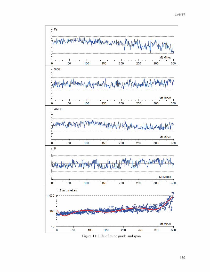
Figure 11 on the following page shows the planned mine operation, over a fifteen year life. The sequence of TBLs selected for weekly production successfully produce ore consistently close to target grade, with the weekly span controlled to a couple of hundred metres, until close to the end of the mine life.

Planning an Iron Ore Mine

158

Figure 9: Trimming the available block list to satisfy multiple criteria

Figure 10: Plot of an initial ABL and final TBL

Everett

159

Figure 11: Life of mine grade and span

Planning an Iron Ore Mine

160

Mining Before being mined, the ore is blasted, using a pattern of drilled blast holes packed with explo-sives. This blasting is done every few days to generate a stock of mineable ore. Samples of ore from the blast holes provide a last minute update to grade estimates, and are used in a regression model to forecast the grade of the potential lump and fines products (Everett & Howard, 2012). Using their forecast grades, each day’s blend is selected from the available blasted ore sources to bring the exponentially smoothed grade back as close as possible to the target grade in each ana-lyte (Everett, 2007). The ore flow is tracked so that comparison of the blast hole grades with the final assays of the corresponding mined ore enables the regression model predicting ore grade from blast hole grade to be periodically updated.

Processing and Transport As ore is mined it is fed into a crusher and then typically railed to a distant port for loading onto a ship. Only after the crushing stage can we reliably measure the ore grade, with a day or two de-lay, so final decisions and forecasting from recent events will be required to ensure adequate grade control of shipped product. Simulation models of alternative configurations are helpful in planning these stages of the production system (Everett, 2010). With simulation models it is pos-sible to explore the effects of alternative production and transport policies. Such models also serve a very useful function in settling disagreements between policy makers and “trying out” suggested approaches, without the cost commitments that would be incurred by trial in the field.

Conclusion We have seen how the block model is a probabilistic data set that provides the evolving infor-mation on which planning and development decisions must be based. The block model, together with the technical, financial and marketing staff, their evolving interpretation of the block model and the unfolding market and technical environments collectively comprise a complex adative system. The necessity to base decisions upon probabilistic inferences from the continually modi-fied data set, generates a continual tension between the cost of gaining more information to re-duce the uncertainty, and the estimated cost of the risk inherent in making decisions under that uncertainty.

Given the considerable benefit in making appropriate decisions in the uncertain environment, it is surprising to find that many decision makers in large mining companies continue to use mislead-ing paradigms. Some of these inappropriate paradigms have been identified in the discussion above: notably the use of quadratic cut-off criteria instead of a composite cut-off, and the under-estimation of ore tonnage by using kriging interpolation, instead of recognising the effect of the increased variability by conditional simulation. A previous paper (Everett, 2012) gave a tentative taxonomy of such paradigm problems (based on Gill, 2010) and provided some further examples from the iron ore mining industry. These examples included the use of sharp constraints instead of continuous objective functions in grade control systems (leading to instability); the treatment of data as hard facts instead of recognising them as probabilistic estimates, and the underestima-tion of assay error, sanctioned by the ISO procedure that successively deletes “outliers” without finding and eliminating their cause.

I have observed that one generator of such problems is the tendency of practitioners to use inter-pretive software, developed elsewhere, that they do not fully understand and which therefore is treated as a “black box” whose output is accepted and believed without any knowledge of how it was generated. This tendency is particularly acute in large companies, where different groups of staff members have narrowly delimited functions, each receiving their input information without a culture of questioning the validity of such inputs.

Everett

161

References Boyle, C. (2009). Multivariate conditional simulation of iron ore deposits – Advantages over models made

using ordinary kriging. Proceedings of Iron Ore 2007, 57-66. Melbourne: The Australasian Institute of Mining and Metallurgy.

Coombes, J., Thomas, G., Glacken, I., & Snowden, V. (2000). Conditional simulation – Which method for mining? Geostats 2000, Cape Town, 1-15. South Africa: Document Transformation Technologies.

Everett, J. E. (2007). Computer aids for production systems management in iron ore mining. International Journal of Production Economics, 110(1), 213-223.

Everett, J. E. (2010). Simulation modeling of an iron ore operation to enable informed planning. Interdisci-plinary Journal of Information, Knowledge, and Management, 5, 101-114. Retrieved from http://www.ijikm.org/Volume5/IJIKMv5p101-114Everett457.pdf

Everett, J. E. (2011). Ore selection and sequencing. Applied Earth Science, 120(3), 130-136.

Everett, J. E. (2012). Paradigm lost. Informing Science: the International Journal of an Emerging Trans-discipline, 15, 35-48. Retrieved from http://www.inform.nu/Articles/Vol15/ISJv15p035-048Everett613.pdf

Everett, J. E., & Howard, T. J. (2012). Predicting finished product properties in the mining industry from pre-extraction data. Applied Earth Science, 120(3), 137-147.

Everett, J. E., & Rimes, M. (2010). A mine-planning model to satisfy long-term grade targets. Applied Earth Science, 119(3), 183-187.

Geoscience Australia. (2012). Australian atlas of minerals resources, mines & processing centres. Re-trieved from http://www.australianminesatlas.gov.au/education/fact_sheets/iron.html

Gill, T. G. (2010). Informing business: Research and education on a rugged landscape. Santa Rosa, Cali-fornia: Informing Science Press.

Gill, T. G., & Cohen, E. (2009). Foundations of Informing Science: 1999-2008. Santa Rosa, California: Informing Science Press.

Krige, D. G. (1951). A statistical approach to some mine valuations and allied problems at the Witwaters-rand. Master's thesis of the University of Witwatersrand, South Africa.

Lord, J. H., & Trendall, A. F. (1976). Iron-ore deposits of Western Australia – Geology and development, circum-pacific energy and mineral resources. AAPG Special Volumes, A175, 410-417.

O'Brien, R. (2009). Australia's iron ore product quality. Geoscience Australia

Richmond, A. (2003). Financially efficient ore selection incorporating grade uncertainty. Mathematical Geology, 35(2), 195-215.

US Geological Survey. (2012). Mineral commodity summaries. Retrieved from http://minerals.usgs.gov/minerals/pubs/commodity/iron_ore/

Planning an Iron Ore Mine

162

Biography Jim Everett began as a research geophysicist at Cambridge and the Aus-tralian National University. His family always said “what are you going to do when you grow up”, so he then joined industry, as a petroleum ex-ploration geophysicist. With a computer background, he was put onto project evaluations. Losing arguments with accountants, he did a couple of Economics and Commerce degrees at the University of Western Aus-tralia (UWA), and found the accountants were usually right. UWA was starting its MBA course and wanted people with industry experience to teach on it. With a young family, fieldwork was now less attractive, so Jim jumped at the chance of returning to academia, spending thirty years in the UWA Business School.

Since retirement as Emeritus Professor of Information Management, he divides his time between research and consulting to Western Australia’s booming mining industry. Most old folk lose their faculties, but he has recently gained one, joining the UWA Earth and Environment Faculty as an Adjunct Professor in the Centre for Exploration Targeting.