Planck 2015 results. XXIV. Cosmology from Sunyaev ...

Astronomy & Astrophysics manuscript no. szcosmo2014 c©ESO 2018February 20, 2018

Planck 2015 results. XXIV. Cosmology from Sunyaev-Zeldovichcluster counts

Planck Collaboration: P. A. R. Ade97, N. Aghanim65, M. Arnaud81, M. Ashdown77, 6, J. Aumont65, C. Baccigalupi95, A. J. Banday108, 11,R. B. Barreiro72, J. G. Bartlett1, 74, N. Bartolo33, 73, E. Battaner110, 111, R. Battye75, K. Benabed66, 107, A. Benoît63, A. Benoit-Lévy27, 66, 107,

J.-P. Bernard108, 11, M. Bersanelli36, 53, P. Bielewicz90, 11, 95, J. J. Bock74, 13, A. Bonaldi75?, L. Bonavera72, J. R. Bond10, J. Borrill16, 101,F. R. Bouchet66, 99, M. Bucher1, C. Burigana52, 34, 54, R. C. Butler52, E. Calabrese104, J.-F. Cardoso82, 1, 66, A. Catalano83, 80, A. Challinor69, 77, 14,

A. Chamballu81, 18, 65, R.-R. Chary62, H. C. Chiang30, 7, P. R. Christensen91, 39, S. Church103, D. L. Clements61, S. Colombi66, 107,L. P. L. Colombo26, 74, C. Combet83, B. Comis83, F. Couchot79, A. Coulais80, B. P. Crill74, 13, A. Curto72, 6, 77, F. Cuttaia52, L. Danese95,

R. D. Davies75, R. J. Davis75, P. de Bernardis35, A. de Rosa52, G. de Zotti49, 95, J. Delabrouille1, F.-X. Désert58, J. M. Diego72, K. Dolag109, 87,H. Dole65, 64, S. Donzelli53, O. Doré74, 13, M. Douspis65, A. Ducout66, 61, X. Dupac42, G. Efstathiou69, F. Elsner27, 66, 107, T. A. Enßlin87,

H. K. Eriksen70, E. Falgarone80, J. Fergusson14, F. Finelli52, 54, O. Forni108, 11, M. Frailis51, A. A. Fraisse30, E. Franceschi52, A. Frejsel91,S. Galeotta51, S. Galli76, K. Ganga1, M. Giard108, 11, Y. Giraud-Héraud1, E. Gjerløw70, J. González-Nuevo22, 72, K. M. Górski74, 112, S. Gratton77, 69,

A. Gregorio37, 51, 57, A. Gruppuso52, J. E. Gudmundsson105, 93, 30, F. K. Hansen70, D. Hanson88, 74, 10, D. L. Harrison69, 77, S. Henrot-Versillé79,C. Hernández-Monteagudo15, 87, D. Herranz72, S. R. Hildebrandt74, 13, E. Hivon66, 107, M. Hobson6, W. A. Holmes74, A. Hornstrup19, W. Hovest87,

K. M. Huffenberger28, G. Hurier65, A. H. Jaffe61, T. R. Jaffe108, 11, W. C. Jones30, M. Juvela29, E. Keihänen29, R. Keskitalo16, T. S. Kisner85,R. Kneissl41, 8, J. Knoche87, M. Kunz20, 65, 3, H. Kurki-Suonio29, 47, G. Lagache5, 65, A. Lähteenmäki2, 47, J.-M. Lamarre80, A. Lasenby6, 77,

M. Lattanzi34, C. R. Lawrence74, R. Leonardi9, J. Lesgourgues67, 106, F. Levrier80, M. Liguori33, 73, P. B. Lilje70, M. Linden-Vørnle19,M. López-Caniego42, 72, P. M. Lubin31, J. F. Macías-Pérez83, G. Maggio51, D. Maino36, 53, N. Mandolesi52, 34, A. Mangilli65, 79, M. Maris51,P. G. Martin10, E. Martínez-González72, S. Masi35, S. Matarrese33, 73, 44, P. McGehee62, P. R. Meinhold31, A. Melchiorri35, 55, J.-B. Melin18,

L. Mendes42, A. Mennella36, 53, M. Migliaccio69, 77, S. Mitra60, 74, M.-A. Miville-Deschênes65, 10, A. Moneti66, L. Montier108, 11, G. Morgante52,D. Mortlock61, A. Moss98, D. Munshi97, J. A. Murphy89, P. Naselsky92, 40, F. Nati30, P. Natoli34, 4, 52, C. B. Netterfield23, H. U. Nørgaard-Nielsen19,

F. Noviello75, D. Novikov86, I. Novikov91, 86, C. A. Oxborrow19, F. Paci95, L. Pagano35, 55, F. Pajot65, D. Paoletti52, 54, B. Partridge46, F. Pasian51,G. Patanchon1, T. J. Pearson13, 62, O. Perdereau79, L. Perotto83, F. Perrotta95, V. Pettorino45, F. Piacentini35, M. Piat1, E. Pierpaoli26,

D. Pietrobon74, S. Plaszczynski79, E. Pointecouteau108, 11, G. Polenta4, 50, L. Popa68, G. W. Pratt81, G. Prézeau13, 74, S. Prunet66, 107, J.-L. Puget65,J. P. Rachen24, 87, R. Rebolo71, 17, 21, M. Reinecke87, M. Remazeilles75, 65, 1, C. Renault83, A. Renzi38, 56, I. Ristorcelli108, 11, G. Rocha74, 13,

M. Roman1?, C. Rosset1, M. Rossetti36, 53, G. Roudier1, 80, 74, J. A. Rubiño-Martín71, 21, B. Rusholme62, M. Sandri52, D. Santos83,M. Savelainen29, 47, G. Savini94, D. Scott25, M. D. Seiffert74, 13, E. P. S. Shellard14, L. D. Spencer97, V. Stolyarov6, 102, 78, R. Stompor1,

R. Sudiwala97, R. Sunyaev87, 100, D. Sutton69, 77, A.-S. Suur-Uski29, 47, J.-F. Sygnet66, J. A. Tauber43, L. Terenzi96, 52, L. Toffolatti22, 72, 52,M. Tomasi36, 53, M. Tristram79, M. Tucci20, J. Tuovinen12, M. Türler59, G. Umana48, L. Valenziano52, J. Valiviita29, 47, B. Van Tent84, P. Vielva72,

F. Villa52, L. A. Wade74, B. D. Wandelt66, 107, 32, I. K. Wehus74, 70, J. Weller109, S. D. M. White87, D. Yvon18, A. Zacchei51, and A. Zonca31

(Affiliations can be found after the references)

Received ; accepted

ABSTRACT

We present cluster counts and corresponding cosmological constraints from the Planck full mission data set. Our catalogue consistsof 439 clusters detected via their Sunyaev-Zeldovich (SZ) signal down to a signal-to-noise ratio of 6, and is more than a factorof 2 larger than the 2013 Planck cluster cosmology sample. The counts are consistent with those from 2013 and yield compatibleconstraints under the same modelling assumptions. Taking advantage of the larger catalogue, we extend our analysis to the two-dimensional distribution in redshift and signal-to-noise. We use mass estimates from two recent studies of gravitational lensing ofbackground galaxies by Planck clusters to provide priors on the hydrostatic bias parameter, (1 − b). In addition, we use lensing ofcosmic microwave background (CMB) temperature fluctuations by Planck clusters as an independent constraint on this parameter.These various calibrations imply constraints on the present-day amplitude of matter fluctuations in varying degrees of tension withthose from the Planck analysis of primary fluctuations in the CMB; for the lowest estimated values of (1− b) the tension is mild, onlya little over one standard deviation, while it remains substantial (3.7σ) for the largest estimated value. We also examine constraintson extensions to the base flat ΛCDM model by combining the cluster and CMB constraints. The combination appears to favour non-minimal neutrino masses, but this possibility does little to relieve the overall tension because it simultaneously lowers the implied valueof the Hubble parameter, thereby exacerbating the discrepancy with most current astrophysical estimates. Improving the precision ofcluster mass calibrations from the current 10 %-level to 1 % would significantly strengthen these combined analyses and provide astringent test of the base ΛCDM model.

Key words. cosmological parameters – large-scale structure of Universe – galaxies: clusters: general – gravitational lensing: weak

? Corresponding authors:A. Bonaldi, [email protected]. Roman, [email protected]

Article number, page 1 of 19

arX

iv:1

502.

0159

7v3

[as

tro-

ph.C

O]

19

Feb

2018

[email protected]

[email protected]

A&A proofs: manuscript no. szcosmo2014

1. Introduction

Galaxy cluster counts are a standard cosmological tool that hasfound powerful application in recent Sunyaev-Zeldovich (SZ)surveys performed by the Atacama Cosmology Telescope (ACT,Swetz et al. 2011; Hasselfield et al. 2013), the South Pole Tele-scope (SPT, Carlstrom et al. 2011; Benson et al. 2013; Re-ichardt et al. 2013; Bocquet et al. 2014), and the Planck satellite1

(Tauber et al. 2010; Planck Collaboration I 2011). The abun-dance of clusters and its evolution are sensitive to the cosmicmatter density, Ωm, and the present amplitude of density fluctua-tions, characterized by σ8, the rms linear overdensity in spheresof radius 8h−1 Mpc. The primary cosmic microwave background(CMB) anisotropies, on the other hand, reflect the density per-turbation power spectrum at the time of recombination. This dif-ference is important because a comparison of the amplitude ofthe perturbations at the two epochs tests the evolution of den-sity perturbations from recombination until today, enabling us tolook for possible extensions to the base ΛCDM model, such asnon-minimal neutrino masses or non-zero curvature.

Launched on 14 May 2009, Planck scanned the entire skytwice a year from 12 August 2009 to 23 October 2013, at angu-lar resolutions from 33′ to 5′with two instruments: the Low Fre-quency Instrument (LFI; Bersanelli et al. 2010; Mennella et al.2011), covering bands centred at 30, 44, and 70 GHz, and theHigh Frequency Instrument (HFI; Lamarre et al. 2010; PlanckHFI Core Team 2011), covering bands centred at 100, 143, 217,353, 545, and 857 GHz.

An initial set of cosmology results appeared in 2013, basedon the first 15.5 months of data (Planck Collaboration I 2014),including cosmological constraints from the redshift distribu-tion of 189 galaxy clusters detected at signal-to-noise (S/N)> 7 (hereafter, our “first analysis” or the “2013 analysis”, PlanckCollaboration XX 2014). The present paper is part of the secondset of cosmology results obtained from the full mission data set;it is based on an updated cluster sample introduced in an accom-panying paper (the PSZ2, Planck Collaboration I 2015).

Our first analysis found fewer clusters than predicted byPlanck’s base ΛCDM model, expressed as a tension betweenthe cluster constraints on (Ωm, σ8) and those from the primaryCMB anisotropies (Planck Collaboration XVI 2014). This couldreflect the need for an extension to the base ΛCDM model or in-dicate that clusters are more massive than determined by the SZsignal-mass scaling relation adopted in 2013.

The cluster mass scale is the largest source of uncertaintyin interpretation of the cluster counts. We based our first analy-sis on X-ray mass proxies that rely on the assumption of hydro-static equilibrium. Simulations demonstrate that this assumptioncan be violated by bulk motions in the gas or by non-thermalsources of pressure (e.g., magnetic fields or cosmic rays, Nagaiet al. 2007; Piffaretti & Valdarnini 2008; Meneghetti et al. 2010).Systematics in the X-ray analyses (e.g., instrument calibration,temperature structure in the gas) could also bias the mass mea-surements significantly (Rasia et al. 2006, 2012). We quantifiedour ignorance of the true mass scale of clusters with a mass biasparameter that was varied over the range 0−30 %, with a baselinevalue of 20 % (see below for the definition of the mass bias), as

1 Planck (http://www.esa.int/Planck) is a project of the Euro-pean Space Agency (ESA) with instruments provided by two scientificconsortia funded by ESA member states and led by Principal Investi-gators from France and Italy, telescope reflectors provided through acollaboration between ESA and a scientific consortium led and fundedby Denmark, and additional contributions from NASA (USA).

suggested by numerical simulations (see the Appendix of PlanckCollaboration XX 2014).

Gravitational lensing studies of the SZ signal-mass relationare particularly valuable in this context because they are inde-pendent of the dynamical state of the cluster (Marrone et al.2012; Planck Collaboration Int. III 2013), although they also,of course, can be affected by systematic effects (e.g., Becker &Kravtsov 2011). New, more precise lensing mass measurementsfor Planck clusters have appeared since our 2013 analysis (vonder Linden et al. 2014b; Hoekstra et al. 2015). We incorporatethese new results as prior constraints on the mass bias in thepresent analysis. Two other improvements over 2013 are the useof a larger cluster catalogue and analysis of the counts in signal-to-noise as well as redshift.

In addition, we apply a novel method to measure clustermasses through lensing of the CMB anisotropies. This method,presented in Melin & Bartlett (2014), enables us to use Planckdata alone to constrain the cluster mass scale. It provides an im-portant independent mass determination, which we compare tothe galaxy lensing results, and one that is representative in thesense that it averages over the entire cluster cosmology sample,rather than a particularly chosen subsample. It is, however, lesswell tested than the other lensing methods because of its novelnature, and we comment on various potential systematics deserv-ing further examination.

Our conventions throughout the paper are as follows. Wespecify cluster mass, M500, as the total mass within a sphereof radius R500, defined as the radius within which the meanmass over-density of the cluster is 500 times the cosmic criti-cal density at its redshift, z: M500 = (4π/3)R3

500[500ρc(z)], withρc(z) = 3H2(z)/(8πG), where H(z) is the Hubble parameter withpresent-day value H0 = h × 100 km s−1 Mpc−1. We give SZ sig-nal strength, Y500, in terms of the Compton y-profile integratedwithin a sphere of radius R500, and we assume that all clustersfollow the universal pressure profile of Arnaud et al. (2010).Density parameters are defined relative to the present-day crit-ical density, e.g., Ωm = ρm/ρc(z = 0) for the total matter density,ρm.

We begin in the next section with a presentation of the Planck2015 cluster cosmology samples. In Sect. 3 we develop ourmodel for the cluster counts in both redshift and signal-to-noise,including a discussion of the scaling relation, the scatter and thesample selection function. Section 4 examines the overall clus-ter mass scale in light of recent gravitational lensing measure-ments; we also present our own calibration of the cluster massscale based on lensing of the CMB temperature fluctuations.Construction of the cluster likelihood and selection of externaldata sets is detailed in Sect. 5. We compare results based on ournew likelihood to the 2013 Planck cluster results in Sect. 6. Wethen present our 2015 cosmological constraints in Sect. 7, sum-marizing and discussing the results in Sect. 8. We examine thepotential impact of different modelling uncertainties in the Ap-pendix.

2. The Planck cosmological samples

We detect clusters across the six highest frequency Planck bands(100 − 857 GHz, Planck Collaboration VII 2015; Planck Col-laboration VIII 2015) using two implementations of the multi-frequency matched filter (MMF3 and MMF1, Melin et al. 2006;Planck Collaboration XXIX 2014) and a Bayesian extension(PwS, Carvalho et al. 2009) that all incorporate the known (non-relativistic) SZ spectral signature and a model for the spatial pro-


http://www.esa.int/Planck

Planck Collaboration: Cosmology from SZ cluster counts

Fig. 1: Mass-redshift distribution of the Planck cosmologicalsamples colour-coded by their signal-to-noise, q. The baselineMMF3 2015 cosmological sample is shown as the small filledcircles. Objects which were in the MMF3 2013 cosmologicalsample are marked by crosses, while those in the 2015 inter-section sample are shown as open circles. The final samples aredefined by q > 6. The mass MYz is the Planck mass proxy (seetext, Arnaud et al. 2015).

file of the signal. The latter is taken to be the so-called “univer-sal pressure profile” from Arnaud et al. (2010) — with the non-standard self-similar scaling — and parameterized by an angularscale, θ500.

We empirically characterize noise (all non-SZ signals) in lo-calized sky patches (10 on a side for MMF3) using the set ofcross-frequency power-spectra. We construct the filters with theresulting noise weights, and we then filter the set of six frequencymaps over a range of cluster scales, θ500, spanning 1–35 arcmin.The filter returns an estimate of Y500 for each scale, based onthe adopted profile template, and sources are finally assignedthe θ500 (and hence Y500) value of the scale that maximizes theirsignal-to-noise. Details are given in Planck Collaboration XXIX(2014) and in an accompanying paper introducing the Planckfull-mission SZ catalogue (PSZ2, Planck Collaboration XXVII2015).

We define two cosmological samples from the general PSZ2catalogues, one consisting of detections by the MMF3 matchedfilter and the other of objects detected by all three methods (theintersection catalogue). Both are defined by a signal-to-noise(denoted q throughout) cut of q > 6. We then apply a mask toremove regions of high dust emission and point sources, leaving65 % of the sky unmasked. The general catalogues, noise mapsand masks can be downloaded from the Planck Legacy Archive.2

The cosmological samples can be easily constructed fromthe PSZ2 union and MMF3 catalogues. The MMF3 cosmologysample is the subsample of the MMF3 catalogue defined by q >6 and for which the entry in the union catalogue has COSMO=’T’.The intersection cosmology sample is defined from the unioncatalogue by the criteria COSMO=’T’, PIPEDET=111, and q > 6.

Fig. 1 shows the distribution of these samples in mass andredshift, together with the 2013 cosmology sample. The masshere is the Planck mass proxy, MYz, defined in Arnaud et al.(2015) (see also Section 7.2.2. in Planck Collaboration XXIX2014) and taken from the PSZ2 catalogue. It is calculated using

2 http://pla.esac.esa.int/pla/

the Planck size-flux posterior contours in conjunction with X-ray priors to break the size-flux degeneracy inherent to the largePlanck beams (see, e.g., Fig. 16 of Planck Collaboration XXVII2015). The samples span masses in the range (2− 10)× 1014 Mand redshifts from z = 0 to 1.3 This quantityMYz is used in theexternal lensing mass calibration measurements, as discussed inSect. 4.

The MMF3 (intersection) sample contains 439 (493) detec-tions. We note that the intersection catalogue has more objectsthan the MMF3 catalogue because of the different definitions ofthe signal-to-noise in the various catalogues. The signal-to-noisefor the intersection catalogue corresponds to the highest signal-to-noise of the three detection algorithms (MMF1, MMF3, orPwS), while for the MMF3 catalogue we use its correspond-ing signal-to-noise. As a consequence, the lowest value for theMMF3 signal-to-noise in the intersection sample is 4.8. We notethat, while being above our detection limit, the Virgo and thePerseus clusters are not part of our samples. This is becauseVirgo is too extended to be blindly detected by our algorithmsand Perseus is close to a masked region.

The 2015 MMF3 cosmology sample contains all but one ofthe 189 clusters of the 2013 MMF3 sample. The missing clusteris PSZ1 980, which falls inside the 2015 point source mask. Six(14) redshifts are missing from the MMF3 (intersection) sample.Our analysis accounts for these by renormalizing the observedcounts to redistribute the missing fraction uniformly across theconsidered redshift range [0,1]. The small number of clusterswith missing redshifts has no significant impact on our results.

We use the MMF3 cosmology sample at q > 6 for our base-line analysis and the intersection sample for consistency checks,as detailed in the Appendix. In particular, we show that the in-tersection sample yields equivalent constraints.

3. Modelling cluster counts

From the theoretical perspective, cluster abundance is a functionof halo mass and redshift, as specified by the mass function. Ob-servationally, we detect clusters in Planck through their SZ sig-nal strength or, equivalently, their signal-to-noise and measuretheir redshift with follow-up observations. The observed clus-ter counts are therefore a function of redshift, z, and signal-to-noise, q. While we restricted our 2013 cosmology analysis to theredshift distribution alone (Planck Collaboration XX 2014), thelarger catalogue afforded by the full mission data set offers thepossibility of an analysis in both redshift and signal-to-noise. Wetherefore develop the theory in terms of the joint distribution ofclusters in the (z, q)-plane and then relate it to the more specificanalysis of the redshift distribution to compare with our previousresults.

3.1. Counts as a function of redshift and signal-to-noise

The distribution of clusters in redshift and and signal-to-noisecan be written as

dNdzdq

=

∫dΩmask

∫dM500

dNdzdM500dΩ

P[q|qm(M500, z, l, b)],

(1)

withdN

dzdM500dΩ=

dNdVdM500

dVdzdΩ

, (2)

3 We fix h = 0.7 and ΩΛ = 1 −Ωm = 0.7 for the mass calculation.


http://pla.esac.esa.int/pla/


i.e., the dark matter halo mass function times the volume el-ement. We adopt the mass function from Tinker et al. (2008)throughout, apart from the Appendix, where we compare to theWatson et al. (2013a) mass function as a test of modelling robust-ness; there, we show that the Watson et al. (2013a) mass functionyields constraints similar to those from the Tinker et al. (2008)mass function, but shifted by about 1σ towards higher Ωm andlower σ8 along the main degeneracy line.

The quantity P[q|qm(M500, z, l, b)] is the distribution of qgiven the mean signal-to-noise value, qm(M500, z, l, b), predictedby the model for a cluster of mass M500 and redshift z lo-cated at Galactic coordinates (l, b).4 This latter quantity is de-fined as the ratio of the mean SZ signal expected of a cluster,Y500(M500, z), as given in Eq. (7), and the detection filter noise,σf[θ500(M500, z), l, b]:

qm ≡ Y500(M500, z)/σf[θ500(M500, z), l, b]. (3)

The filter noise depends on sky location (l, b) and the clusterangular size, θ500, which introduces additional dependence onmass and redshift. More detail on σf can be found in PlanckCollaboration XX (2014) (see in particular figure 4 therein).

The distribution P[q|qm] incorporates noise fluctuations andintrinsic scatter in the actual cluster Y500 around the mean value,Y500(M500, z), predicted from the scaling relation. We discuss thisscaling relation and our log-normal model for the intrinsic scatterbelow, and Sect. 4 examines the calibration of the overall massscale for the scaling relation.

The redshift distribution of clusters detected at q > qcat is theintegral of Eq. (1) over signal-to-noise,

dNdz

(q > qcat) =

∫ ∞

qcat

dqdN

dzdq

=

∫dΩ

∫dM500 χ(M500, z, l, b)

dNdzdM500dΩ

, (4)

with

χ(M500, z, l, b) =

∫ ∞

qcat

dq P[q|qm(M500, z, l, b)]. (5)

Equation (4) is equivalent to the expression used in our 2013analysis if we write it in the form

χ =

∫d ln Y500

∫dθ500P(ln Y500, θ500|z,M500) χ(Y500, θ500, l, b),

(6)

where χ(Y500, θ500, l, b) is the survey selection function atq > qcat in terms of true cluster parameters (Sect. 3.3), andP(ln Y500, θ500|z,M500) is the distribution of these parametersgiven cluster mass and redshift. We specify the relation betweenEq. (5) and Eq. (6) in the next section.

3.2. Observable-mass relations

A crucial element of our modelling is the relation between clus-ter observables, Y500 and θ500, and halo mass and redshift. Dueto intrinsic variations in cluster properties, this relation is de-scribed by a distribution function, P(ln Y500, θ500|M500, z), whosemean values are specified by the scaling relations Y500(M500, z)and θ500(M500, z).4 This form assumes, as we do throughout, that the distribution de-pends on z and M500 only through the mean value qm, specifically, thatthe intrinsic scatter, σlnY, of Eq. (9) is constant.

Table 1: Summary of SZ-mass scaling-law parameters (seeEq. 7).

Parameter Value

log Y∗ −0.19 ± 0.02α a 1.79 ± 0.08β b 0.66 ± 0.50σ c

ln Y 0.173 ± 0.023

a Except when specified, α is constrained by this prior in our one-dimensional likelihood over N(z), but left free in our two-dimensionallikelihood over N(z, q).

b We fix β to its central value throughout, except when examining mod-elling uncertainties in the Appendix.

c The value is the same as in our 2013 analysis, given here in terms ofthe natural logarithm and computed from σlog Y = 0.075 ± 0.01.

We use the same form for these scaling relations as in our2013 analysis:

E−β(z) D2

A(z)Y500

10−4 Mpc2

= Y∗

[h

0.7

]−2+α [(1 − b) M500

6 × 1014 M

]α, (7)

and

θ500 = θ∗

[h

0.7

]−2/3 [(1 − b) M500

3 × 1014M

]1/3

E−2/3(z)[

DA(z)500 Mpc

]−1

, (8)

where θ∗ = 6.997 arcmin, and fiducial ranges for the parametersY∗, α, and β are listed in Table 1; these values are identical tothose used in our 2013 analysis. Unless otherwise stated, we useGaussian distributions with mean and standard deviation givenby these values as prior constraints; one notable exception willbe when we simultaneously fit for α and cosmological param-eters. In the above expressions, DA(z) is the angular diameterdistance and E(z) ≡ H(z)/H0.

These scaling relations have been established by X-ray ob-servations, as detailed in the Appendix of Planck CollaborationXX (2014), and rely on mass determinations, MX, based on hy-drostatic equilibrium of the intra-cluster gas. The “mass bias”parameter, b, assumed to be constant in both mass and redshift,allows for any difference between the X-ray determined massesand true cluster halo mass: MX = (1 − b)M500. This is discussedat length in Sect. 4.

We adopt a log-normal5 distribution for Y500 around its meanvalue Y500, and a delta function for θ500 centred on θ500:

P(ln Y500, θ500|M500, z) =1

√2πσlnY

e− ln2(Y500/Y500)/(2σ2lnY)

× δ[θ500 − θ500], (9)

where Y500(M500, z) and θ500(M500, z) are given by Eqs. (7) and(8). The δ-function maintains the empirical definition of R500 thatis used in observational determinations of the profile.

We can now specify the relation between Eqs. (5) and (6) bynoting that

P[q|qm(M500, z, l, b)] =

∫d ln qmP[q|qm]P[ln qm|qm], (10)

5 In this paper, “ln" denotes the natural logarithm and "log" the loga-rithm to base 10; the expression is written in terms of the natural loga-rithm.



where P[q|qm] is the distribution of observed signal-to-noise, q,given the model value, qm. The second distribution represents in-trinsic cluster scatter, which we write in terms of our observable-mass distribution, Eq. (9), as

P[ln qm|qm] =

∫dθ500P[ln Y500(ln qm, θ500, l, b), θ500|M500, z]

=1

√2πσlnY

e− ln2(qm/qm)/2σ2lnY . (11)

Performing the integral of Eq. (5), we find

χ =

∫d ln qmP[ln qm|qm]χ(Y500, θ500, l, b), (12)

with the definition of our survey selection function

χ(Y500, θ500, l, b) =

∫ ∞

qcat

dqP[q|qm(Y500, θ500, l, b)]. (13)

We then reproduce Eq. (6) by using the first line of Eq. (11) andEq. (3).

3.3. Selection function and survey completeness

The fundamental quantity describing the survey selection isP[q|qm], introduced in Eq. (10). It gives the observed signal-to-noise, used to select SZ sources, as a function of model (“true”)cluster parameters through qm(Y500, θ500, l, b), and it defines the“survey selection function” χ(Y500, θ500, l, b) via Eq. (13). Wecharacterize the survey selection in two ways. The first is with ananalytical model and the second employs a Monte Carlo extrac-tion of simulated sources injected into the Planck maps. In addi-tion, we perform an external validation of our selection functionusing known X-ray clusters.

The analytical model assumes pure Gaussian noise, in whichcase we simply have P[q|qm] = e−(q−qm)2/2/

√2π. The survey se-

lection function is then given by the error function (and we referto this as the ERF completeness function),

χ(Y500, θ500, l, b) =12

[1 − erf

(qcat − qm(Y500, θ500, l, b)

√2

)]. (14)

This model can be applied to a catalogue with well-defined noiseproperties (i.e., σf), such as our MMF3 catalogue, but not to theintersection catalogue based on the simultaneous detection withthree different methods. This is our motivation for choosing theMMF3 catalogue as our baseline.

In the Monte Carlo approach, we inject simulated clustersdirectly into the Planck maps and (re)extract them with the com-plete detection pipeline. Details are given in the accompanying2015 SZ catalogue paper, Planck Collaboration XXVII (2015).This method provides a more comprehensive description of thesurvey selection by accounting for a variety of effects beyondnoise. In particular, we vary the shape of the SZ profile at fixedY500 and θ500 to quantify its effect on catalogue completeness.The difference between the Monte-Carlo and ERF complete-ness results in a change in modelled number counts of typically∼ 2.5% (with a maximum of 9%) in each redshift bin.

We also perform an external check of the survey complete-ness using known X-ray clusters from the Meta Catalogue of X-ray Clusters (MCXC) compilation (Piffaretti et al. 2011) and alsoSPT clusters from Bleem et al. (2014). Details are given in the2015 SZ catalogue paper, Planck Collaboration XXVII (2015).For the MCXC compilation, we rely on the expectation that at

redshifts z < 0.2 any Planck-detected cluster should be found inone of the ROSAT catalogues (Chamballu et al. 2012) because atlow redshift ROSAT probes to lower masses than Planck.6 TheMCXC catalogue provides a truth table, replacing the input clus-ter list of the simulations, and we compute completeness as theratio of objects in the cosmology catalogue to the total numberof clusters. As discussed in Planck Collaboration XXVII (2015),the results are consistent with Gaussian noise and bound the pos-sible effect of profile variations. We arrive at the same conclusionwhen applying the technique to the SPT catalogue.

Planck Collaboration XXVII (2015) discusses completenesschecks in greater detail. One possible source of bias is thepresence of correlated IR emission from cluster member galax-ies. Planck Collaboration XXIII (2015) suggests that IR pointsources may contribute significantly to the cluster SED at thePlanck frequencies, especially at higher redshift. The potentialimpact of this effect warrants further study in future work.

We thus have different estimations of the selection functionfor MMF3 and the intersection catalogues. We test the sensitiv-ity of our cosmological constraints to the selection function inthe Appendix by comparing results obtained with the differentmethods and catalogues. We find that our results are insensitiveto the choice of completeness model (Fig A.1), and we thereforeadopt the analytical ERF completeness function for simplicitythroughout the paper.

4. The cluster mass scale

The characteristic mass scale of our cluster sample is the criti-cal element in our analysis of the counts. It is controlled by themass bias factor, 1 − b, accounting for any difference betweenthe X-ray mass proxies used to establish the scaling relationsand the true (halo) mass: MX = (1 − b)M500. Such a differencecould arise from cluster physics (such as a violation of hydro-static equilibrium or temperature structure in the gas, Rasia et al.2006, 2012, 2014), from observational effects (e.g., instrumentalcalibration), or from selection effects biasing the X-ray samplesrelative to SZ- or mass-selected samples (Angulo et al. 2012).

In our 2013 analysis, we adopted a flat prior on the mass biasover the range 1 − b = [0.7, 1.0], with a reference model definedby 1−b = 0.8. This was motivated by a comparison of the Y−MXrelation with published Y − M relations derived from numericalsimulations, as detailed in the Appendix of Planck CollaborationXX (2014); this estimate was consistent with most (although notall) predictions for any violation of hydrostatic equilibrium, aswell as observational constraints from the available lensing ob-servations. Effects other than cluster physics can contribute tothe mass bias, as discussed in our earlier paper, and as empha-sized by the survey of cluster multi-band scaling relations byRozo et al. (2014a,b,c).

The mass bias was the largest uncertainty in our 2013 anal-ysis, and it severely hampered understanding of the tensionfound between constraints from the primary CMB and the clustercounts. Here, we incorporate new lensing mass determinations ofPlanck clusters to constrain the mass bias. We also apply a novelmethod to measure object masses based on lensing of CMB tem-perature anisotropies behind clusters (Melin & Bartlett 2014).These constraints are used as prior information in our analysisof the counts. As we will see, however, uncertainty in the mass

6 In fact, this expectation is violated to a small degree. As discussedin Planck Collaboration XXVII (2015), there appears to be a small pop-ulation of X-ray under-luminous clusters.



bias remains our largest source of uncertainty, mainly becausethese various determinations continue to differ by up to 30 %.

In general, the mass bias could depend on cluster mass andredshift, although we will model it by a constant in the following.Our motivation is one of practicality: the limited size and preci-sion of current lensing samples makes it difficult to constrainany more than a constant value, i.e., the overall mass scale ofour catalogue. Large lensing surveys like Euclid, WFIRST, andthe Large Synoptic Survey Telescope, as well as CMB lensing,will improve this situation in coming years.

4.1. Constraints from gravitational shear

Several cluster samples with high quality gravitational shearmass measurements have appeared since 2013. Among these,the Weighing the Giants (WtG, von der Linden et al. 2014a),CLASH (Postman et al. 2012; Merten et al. 2014; Umetsu et al.2014), and Canadian Cluster Comparison Project (CCCP, Hoek-stra et al. 2015) programmes offer constraints on our mass biasfactor, 1 − b, through direct comparison of the lensing masses tothe Planck mass proxy, MYz.

The analysis by the WtG programme of 22 clusters from the2013 Planck cosmology sample yields 1 − b = 0.688 ± 0.072.Their result lies at the very extreme of the range explored inPlanck Collaboration XX (2014) and would substantially re-duce the tension found between primary CMB and galaxy clus-ter constraints. Hoekstra et al. (2015) report a smaller bias of1−b = 0.78±0.07 (stat) ±0.06 (sys) for a set of 20 common clus-ters, which is in good agreement with the fiducial value adoptedin our 2013 analysis. In our new analysis we add the statisticaland systematic uncertainties in quadrature (see Table 2).

The two samples overlap, but not completely, and, as dis-cussed in detail by Hoekstra et al. (2015), there are numerousdifferences between the two analyses. These include treatment ofsource redshifts, contamination by cluster members and methodsof extracting a mass estimate from the lensing data. And whilethe two mass calibrations differ in a way that attracts particularattention in the present context, they are statistically consistent,separated by about one standard deviation.

4.2. Constraints from CMB lensing

Measuring cluster mass through CMB lensing (Lewis & Challi-nor 2006) has been discussed in the literature for some time sincethe study performed by Zaldarriaga & Seljak (1999). We applya new technique for measuring cluster masses through lensingof CMB temperature anisotropies (Melin & Bartlett 2014), al-lowing us to calibrate the scaling relations using only Planckdata. This is a valuable alternative to the galaxy lensing observa-tions because it is independent and affected by different possiblesystematics. Additionally, we can apply it to the entire clustersample to obtain a mass calibration representative of an SZ flux-selected sample. Similar approaches using CMB lensing to mea-sure halo masses were recently applied by SPT (Baxter et al.2014) and ACT (Madhavacheril et al. 2014).

Our method first extracts a clean CMB temperature map witha constrained internal linear combination (ILC) of the Planckfrequency channels in the region around each cluster; the ILC isconstrained to nullify the SZ signal from the clusters themselvesand provide a clean CMB map of 5 arcmin resolution. Using aquadratic estimator on the CMB map, we reconstruct the lensingpotential in the field and then filter it to obtain an estimate of thecluster mass. The filter is an NFW profile (Navarro et al. 1997)

Fig. 2: Cluster mass scale determined by CMB lensing. We showthe ratio of cluster lensing mass, Mlens, to the SZ mass proxy,MYz, as a function of the mass proxy for clusters in the MMF32015 cosmology sample. The cluster mass is measured throughlensing of CMB temperature anisotropies in the Planck data(Melin & Bartlett 2014). Individual mass measurements havelow signal-to-noise, but we determine a mean ratio for the sam-ple of Mlens/MYz = 1/(1 − b) = 0.99 ± 0.19. For clarity, onlysome of the error bars are plotted (see text).

with scale radius set by the Planck mass proxy for each clus-ter, and designed to return an estimate of the ratio Mlens/MYz,where MYz is the Planck SZ mass proxy. These individual mea-surements are corrected for any mean-field bias by subtractingidentical filter measurements on blank fields; this accounts foreffects of apodization over the cluster fields and correlated noise.The technique has been tested on realistic simulations of Planckfrequency maps. More detail can be found in Melin & Bartlett(2014).

Figure 2 shows Mlens/MYz as a function of MYz for all clus-ters in the MMF3 cosmology sample. Each point is an individualcluster.7 For clarity, only some of the error bars on the ratio areshown; the error bars vary from 1.8 at the high mass end to 8.5at the low mass end, with a median of 4.2. There is no indicationof a correlation between the ratio and MYz, and we therefore fitfor a constant ratio of Mlens/MYz by taking the weighted mean(using the individual measurement uncertainties as provided bythe filter) over the full data set. If the ratio differs from unity,we apply a correction to account for the fact that our filter aper-ture was not perfectly matched to the clusters. The correction iscalculated assuming an NFW profile and is of the order of onepercent.

The final result is 1/(1− b) = 0.99± 0.19, traced by the blueband in the figure. We note that the method constrains 1/(1 −b) rather than 1 − b as in the case of the shear measurements.The calculated uncertainty on the weighted mean is consistentwith a bootstrap analysis, where we create new catalogues ofthe same size as the original by sampling objects from the fullcatalogue with replacement; the uncertainty from the bootstrapis then taken as the standard deviation of the bootstrap means.

The uncertainty 0.19 is statistical. Melin & Bartlett (2014)quote an uncertainty of 0.28 for the 62 ESZ-XMM clustersbased on simulations including only tSZ, kSZ, primary CMB

7 The values can be negative due to noise fluctuations and the lowsignal-to-noise of the individual measurements.



Table 2: Summary of mass scale priors

Prior name Quantity Value and Gaussian errorsWeighing the Giants (WtG) 1 − b 0.688 ± 0.072Canadian Cluster ComparisonProject (CCCP) 1 − b 0.780 ± 0.092CMB lensing (CMBlens) 1/(1 − b) 0.99 ± 0.19Baseline 2013 1 − b 0.8 [−0.1,+0.2]

Notes. For CCCP, we use the value determined for Planck clustersat S/N> 7 (Hoekstra et al. 2015, left column of p. 706) and we addin quadrature the statistical (0.07) and systematic (0.06) uncertainties.CMB lensing directly measures 1/(1 − b), which we implement in ouranalysis; purely for reference, this constraint translates approximatelyto 1 − b = 1.01+0.24

−0.16. The last line shows the 2013 baseline — a ref-erence model defined by 1 − b = 0.8 with a flat prior in the [0.7, 1]range.

and instrumental noise. Scaling this number to 433 (numberof objects with a redshift in the cosmological sample) gives0.28

√62/433 ≈ 0.11, in broad agreement with our value of

0.19. The difference can likely be attributed to the fact that thePlanck cosmological sample is on average less massive than theESZ-XMM sample, and that the Planck maps are more complexthan the model adopted in Melin & Bartlett (2014).

We have obtained a 5σ measurement of the sample massscale using CMB lensing. We emphasize, however, that themethod is new and under development. A number of potentialsystematic effects require further study, including cluster mis-centring and mismatch between filter shape and actual clusterprofiles; these would tend to reduce the observed masses fromtheir true values. On the other hand, effects such as contributionsfrom mass correlated on large scales with the clusters (e.g., fila-ments or neighbouring halos) and contamination by infrared andradio sources could increase the observed signal. We are exam-ining these issues in a study of the ESZ-XMM sample that willbe published at a later date.

4.3. Summary

The three mass bias priors are summarized in Table 2, and wewill extract cosmological constraints from each one. We favourthese three lensing results because of their direct comparisonto the Planck mass proxy. We will assume Gaussian distribu-tions for 1 − b (gravitational shear) or 1/(1 − b) (CMB lensing),with standard deviations given by the error column. We adopt theCCCP mass calibration as our baseline, and give the CMB lens-ing result less weight in our interpretation because of its noveltyand the ongoing studies of the issues mentioned in the previoussection.

5. Analysis methodology

5.1. Likelihood

Our 2013 analysis employed a likelihood built on the cluster red-shift distribution, dN/dz. With the larger 2015 catalogue, ourbaseline likelihood is now constructed on counts in the (z, q)-plane. We divide the catalogue into bins of size ∆z = 0.1 (10bins) and ∆ log q = 0.25 (5 bins), each with an observed numberN(zi, q j) = Ni j of clusters. Modelling the observed counts, Ni j,

as independent Poisson random variables, our log-likelihood is

ln L =

NzNq∑i, j

[Ni j ln Ni j − Ni j − ln[Ni j!]

], (15)

where Nz and Nq are the total number of redshift and signal-to-noise bins, respectively. The mean number of objects in each binis predicted by theory according to Eq. (1):

Ni j =dN

dzdq(zi, q j)∆z∆q, (16)

which depends on the cosmological (and cluster modelling)parameters. In practice, we use a Monte Carlo Markov chain(MCMC) to map the likelihood surface around the maximumand establish confidence limits.

Eq. (15) assumes that the bins are uncorrelated, while a morecomplete description would include correlations due to large-scale clustering. In practice, our cluster sample contains mostlyhigh mass systems for which the impact of these effects is weak(e.g., Hu & Kravtsov 2003, in particular their figure 4 for theimpact on constraints in the (Ωm,σ8) plane).

5.2. External data sets

Cluster counts cannot constrain all pertinent cosmological pa-rameters; they are most sensitive to Ωm and σ8, and whenanalysing the counts alone we must apply additional observa-tional constraints as priors on other parameters. For this pur-pose, we adopt Big Bang nucleosynthesis (BBN) constraintsfrom Steigman (2008), Ωbh2 = 0.022±0.002 (for a recent reviewon BBN, see Olive 2013), and constraints from baryon acous-tic oscillations (BAO). The latter combine the 6dF Galaxy Sur-vey (Beutler et al. 2011), the SDSS Main Galaxy Sample (Pad-manabhan et al. 2012; Anderson et al. 2012) and the BOSSDR11 (Anderson et al. 2014). We refer the reader to Sect. 5.2 inPlanck Collaboration XIII (2015) for details of the combination.We also include a prior on ns from Planck Collaboration XVI(2014), ns = 0.9624±0.014. When explicitly specified in the text,we add the supernovæ constraint from SNLS-II and SNLS3: theJoint Light-curve Analysis constraint (JLA, Betoule et al. 2014).The BAO are particularly sensitive to H0, while the supernovæallow precise constraints on the dark energy equation-of-stateparameter, w.

6. Comparison to 2013

We begin by verifying consistency with the results of PlanckCollaboration XX (2014) (Sect. 6.1) based on the one-dimensional likelihood over the redshift distribution, dN/dz(Eq. 4). We then examine the effect of changing to the full two-dimensional likelihood, dN/dzdq (Eq. 1) in Sect. 6.2. For thispurpose we compare constraints on the total matter density, Ωm,and the linear-theory amplitude of the density perturbations to-day, σ8, using the cluster counts in combination with externaldata and fixing the mass bias. The two-dimensional likelihooddN/dzdq is then adopted as the baseline in the rest of the paper.

6.1. Constraints on Ωm and σ8: one-dimensional analysis

Figure 3 presents constraints from the MMF3 cluster countscombined with the BAO and BBN priors of Sect. 5.2; we re-fer to this data combination as “SZ+BAO+BBN”. To compareto results from our 2013 analysis (the grey, filled ellipses), we



use a one-dimensional likelihood based on Eq. (4) over the red-shift distribution and have adopted the reference scaling relationof 2013, i.e., Eqs. (7) and (8), with the mass bias value fixed to1 − b = 0.8. For the present comparison, we use the updatedBAO constraints discussed in Sect. 5.2; these are stronger thanthe BAO constraints used in the 2013 analysis, and the grey con-tours shown here are consequently smaller than in Planck Col-laboration XX (2014).

Limiting the 2015 catalogue to q > 8.5 produces a sam-ple with 190 clusters, similar to the 2013 cosmology catalogue(189 objects). The two sets of constraints demonstrate good con-sistency, and they remain consistent while becoming tighter aswe decrease the signal-to-noise threshold of the 2015 catalogue.Under similar assumptions, our 2015 analysis thus confirms the2013 results reported in Planck Collaboration XX (2014).

The area of the ellipse from q = 8.5 to q = 6 decreases bya factor of 1.3. This is substantially less than the factor of 2.3expected from the ratio of the number of objects in the two sam-ples. The difference may be related to the decreasing goodness-of-fit of the best model as the signal-to-noise decreases. Whenincorporated, the uncertainty on the mass calibration 1 − b willalso restrict the reduction of the ellipse area.

Figure 4 overlays the observed cluster redshift distributionon the predictions from the best-fit model in each case. We seethat the models do not match the counts in the second and thirdredshift bins (counting from z = 0), and that the discrepancy,already marginally present at the high signal-to-noise cut cor-responding to the 2013 catalogue, becomes more pronouncedtowards the lower signal-to-noise thresholds. This discrepancycannot be attributed to redshift errors in the first bins becausethe majority of the redshifts are spectroscopic and the size ofthe bins is large (∆z = 0.1); for example, the first two redshiftbins contain 208 clusters, of which 200 have spectroscopic red-shifts. The dependence on signal-to-noise may suggest that thedata prefer a different slope, α, of the scaling relation than al-lowed by the prior of Table 1. We explore the effect of relaxingthe X-ray prior on α in the next section.

6.2. Constraints on Ωm and σ8: two-dimensional analysis

In Fig. 5 we compare constraints from the one- and two-dimensional likelihood with α either free or with the priorof Table 1. For this comparison, we continue with the“SZ+BAO+BBN” data set, but adopt the CCCP prior for themass bias and only consider the full 2015 MMF3 catalogue atq > 6.

The grey and black contours and lines in Fig. 5 show resultsfrom the one-dimensional likelihood fit to the redshift distribu-tion using, respectively, the X-ray prior on α and leaving α free.The redshift counts do indeed prefer a steeper slope, with a pos-terior of α = 2.23 ± 0.18 in the latter case and a shift of theconstraints along their degeneracy ridges. To explore this prefer-ence, we split the analysis into low and high redshift bin sets di-vided at z = 0.2, finding that neither the high nor the low redshiftbin set prefers the steeper slope by itself; it appears only whenanalyzing all the bins. As described further in the Appendix,there is a subtle interplay between parameters that is masked bythe degeneracies and difficult to interpret with the present dataset.

A related issue is the acceptability of the model fit. Wedefine a generalized χ2 measure of goodness-of-fit as χ2 =∑Nz

i N−1i

(Ni − Ni

)2, determining the probability to exceed (PTE)

the observed value using Monte Carlo simulations of Poisson

0.25 0.30 0.35 0.40Ωm

0.70

0.74

0.78

0.82

σ8

PSZ2, q=6PSZ2, q=7PSZ2, q=8.5PSZ1, q=7

Fig. 3: Contours at 95 % for different signal-to-noise thresholds,q = 8.5, 7, and 6, applied to the 2015 MMF3 cosmology sam-ple for the SZ+BAO+BBN data set. The contours are compati-ble with the 2013 constraints (Planck Collaboration XX 2014),shown as the filled, light grey ellipses at 68 and 95 % (for theBAO and BBN priors of Sect 5.2; see text). The 2015 cataloguethresholded at q > 8.5 has a similar number of clusters (190)as the 2013 catalogue (189). This comparison is made using theanalytical error-function model for completeness and adopts thereference observable-mass scaling relation of the 2013 analysis(1 − b = 0.8, see text). The redshift distributions of the best-fitmodels are shown in Fig. 4. For this figure and Fig. 4, we use theone-dimensional likelihood over the redshift distribution, dN/dz(Eq. 4).

statistics for each bin with the best-fit model mean Ni. The ob-served value of the fit drops from 17 (PTE = 0.07) with the X-rayprior, to 15 (PTE = 0.11) when leaving α free. When leaving αfree, Ωm increases and σ8 decreases, following their correlationwith α shown by the contours, and their uncertainty increasesdue to the added parameter.

The two-dimensional likelihood over dN/dzdq better con-strains the slope when α is free, as shown by the violet curvesand contours. In this case, the preferred value drops back towardsthe X-ray prior: α = 1.89 ± 0.11, just over 1σ from the centralX-ray value. Re-imposing the X-ray prior on α with the two-dimensional likelihood (blue curves) does little to change theparameter constraints. Although the one-dimensional likelihoodprefers a steeper slope than the X-ray prior, the two-dimensionalanalysis does not, and the cosmological constraints remain ro-bust to varying α.

We define a generalized χ2 statistic as described above, nowover the two-dimensional bins in the (z, q)-plane. This general-ized χ2 for the fit with the X-ray prior is 43 (PTE = 0.28), com-pared to χ2 = 45 (PTE = 0.23) when α is a free parameter.

Fig. 6 displays the redshift distribution of the best-fit modelsin all four cases. Despite their apparent difficulty in matchingthe second and third redshift bins, the PTE values suggest thatthese fits are moderately good to acceptable. We note that, asmentioned briefly in Sect. 5.1, clustering effects will increasethe scatter in each bin slightly over the Poisson value we haveassumed, causing our quoted PTE values to be somewhat smallerthan the true ones.



0.0 0.2 0.4 0.6 0.8 1.0z

020

4060

8010

012

014

0N

(z)

best fit q=6best fit q=7best fit q=8.5MMF3 q=6MMF3 q=7MMF3 q=8.5

Fig. 4: Comparison of observed counts (points with error bars)with predictions of the best-fit models (solid lines) from theone-dimensional likelihood for three different thresholds appliedto the 2015 MMF3 cosmology sample. The mismatch betweenobserved and predicted counts in the second and third lowestredshift bins, already noticed in the 2013 analysis, increases atlower thresholds, q. The best-fit models are defined by the con-straints shown in Fig. 3. For this figure and Fig. 3, we use ourone-dimensional likelihood over the redshift distribution, dN/dz(Eq. 4), with the mass biased fixed at (1 − b) = 0.8.

0.25 0.31 0.38 0.44

N(z,q) α freeN(z,q) α constrainedN(z) α freeN(z) α constrained

0.25 0.31 0.38 0.44

1.7

2.1

2.5

α

1.7 2.1 2.5

0.25 0.31 0.38 0.44

0.65

0.75

0.85

σ8

1.7 2.1 2.5 0.65 0.75 0.85

0.25 0.31 0.38 0.44Ωm

6267

7277

H0

1.7 2.1 2.5α

0.65 0.75 0.85σ8

62 67 72 77H0

Fig. 5: Comparison of constraints from the one-dimensional(dN/dz) and two-dimensional (dN/dzdq) likelihoods on cosmo-logical parameters and the scaling relation mass exponent, α.This comparison uses the MMF3 catalogue, the CCCP prior onthe mass bias and the SZ+BAO+BBN data set. The correspond-ing best-fit model redshift distributions are shown in Fig. 6.

7. Cosmological constraints 2015

We extract constraints on Ωm and σ8 from the cluster counts incombination with external data, imposing the different clustermass scale calibrations as prior distributions on the mass bias.In Sect. 7.1, we compare our new constraints to and then com-bine them with those from the CMB anisotropies in the baseΛCDM model. We study parameter extensions to the base modelin Sect. 7.2. In the following, we adopt as our baseline the 2015

0.0 0.2 0.4 0.6 0.8 1.0z

020

4060

8010

012

014

016

0N

(z)

N(z,q) best fit (CCCP, α constrained)N(z,q) best fit (CCCP, α free)N(z) best fit (CCCP, α constrained)N(z) best fit (CCCP, α free)observed counts

Fig. 6: Redshift distribution of best-fit models from the fouranalysis cases shown in Fig. 5. The observed counts in theMMF3 catalogue (q > 6) are plotted as the red points with errorbars, and as in Fig. 5 we adopt the CCCP mass prior with theSZ+BAO+BBN data set.

two-dimensional SZ likelihood with the CCCP mass bias prior,α free and β = 2/3 fixed in Eq. (7). All quoted intervals are 68%confidence and all upper/lower limits are 95% confidence.

7.1. Base ΛCDM

7.1.1. Constraints on Ωm and σ8: comparison to primaryCMB parameters

Our 2013 analysis brought to light tension between constraintson Ωm andσ8 from the cluster counts and those from the primaryCMB in the base ΛCDM model. In that analysis, we adopted aflat prior on the mass bias over the range 1−b = [0.7, 1.0], with areference model defined by 1−b = 0.8 (see discussion in the ap-pendix of Planck Collaboration XX 2014). Given the good con-sistency between the 2013 and 2015 cluster results (Fig. 3), weexpect the tension to remain under the same assumptions con-cerning the mass bias.

Figure 7 compares our 2015 cluster constraints (MMF3SZ+BAO+BBN) to those for the base ΛCDM model from thePlanck CMB anisotropies. The cluster constraints, given thethree different priors on the mass bias, are shown by the filledcontours at 68 and 95 % confidence, while the dashed blackcontours give the Planck TT,TE,EE+lowP constraints (hereafterPlanck primary CMB, Planck Collaboration XIII 2015); the greyshaded regions add BAO to the CMB. The central value of theWtG mass prior lies at the extreme end of the range used in2013 (i.e., 1 − b = 0.7); with its uncertainty range extendingeven lower, the tension with primary CMB is greatly reduced, aspointed out by von der Linden et al. (2014b). With similar uncer-tainty but a central value shifted to 1− b = 0.78, the CCCP massprior results in greater tension with the primary CMB. The lens-ing mass prior, finally, implies little bias and hence much greatertension.

The red contours present results from a joint analysis of thecluster counts and the Planck lensing power spectrum (PlanckCollaboration XV 2015), adopting our external priors on ns andΩbh2 with the mass bias parameter free and α constrained bythe X-ray prior. It is interesting to note that these constraints arefully independent of those from the primary CMB, but are in



Table 3: Summary of Planck 2015 cluster cosmology constraints

Data σ8

(Ωm0.31

)0.3Ωm σ8

WtG + BAO + BBN 0.806 ± 0.032 0.34 ± 0.03 0.78 ± 0.03CCCP + BAO + BBN [Baseline] 0.774 ± 0.034 0.33 ± 0.03 0.76 ± 0.03CMBlens + BAO + BBN 0.723 ± 0.038 0.32 ± 0.03 0.71 ± 0.03CCCP + H0 + BBN 0.772 ± 0.034 0.31 ± 0.04 0.78 ± 0.04

Notes. The constraints are obtained for our baseline model: the two-dimensional likelihood over the MMF3 catalogue (q > 6) with α free andβ = 2/3 fixed in Eq. (7).

0.25 0.30 0.35 0.40 0.45 0.50 0.55Ωm

0.60

0.68

0.76

0.84

0.92

σ8

CMBSZ+Lensing PSCMB+BAOSZα+BAO (WtG)SZα+BAO (CCCP)SZα+BAO (CMBlens)

Fig. 7: Comparison of constraints from the CMB to those fromthe cluster counts in the (Ωm, σ8)-plane. The green, blue and vi-olet contours give the cluster constraints (two-dimensional like-lihood) at 68 and 95 % for the WtG, CCCP, and CMB lens-ing mass calibrations, respectively, as listed in Table 2. Theseconstraints are obtained from the MMF3 catalogue with theSZ+BAO+BBN data set and α free (hence the SZα notation).Constraints from the Planck TT, TE, EE+lowP CMB likelihood(hereafter, Planck primary CMB) are shown as the dashed con-tours enclosing 68 and 95 % confidence regions (Planck Collab-oration XIII 2015), while the grey shaded region also includesBAO. The red contours give results from a joint analysis of thecluster counts and the Planck lensing power spectrum (PlanckCollaboration XV 2015), adopting our external priors on ns andΩbh2 with the mass bias parameter free and α constrained by theX-ray prior (hence the SZ notation without the subscript α).

good agreement with them, favouring only slightly lower valuesfor σ8.

Table 3 summarizes our cluster cosmology constraints for thebase ΛCDM model for the different mass bias priors. We givethe marginalized constraints on Ωm and σ8, as well as their com-bination that is most tightly constrained by the cluster counts.In addition, in the last line we list constraints when replacingthe BAO prior by a prior on H0 from direct local measurements(Riess et al. 2011): H0 = 73.8 ± 2.4 km s−1 Mpc−1.

7.1.2. Joint Planck 2015 primary CMB and clusterconstraints

Mass bias required by the primary CMB In Fig. 8 we comparethe three prior distributions to the mass bias required by the pri-mary CMB. The latter is obtained as the posterior on 1−b from ajoint analysis of the MMF3 cluster counts and the CMB with the

0.4 0.6 0.8 1.0 1.2 1.4 1.61−b

0.0

0.2

0.4

0.6

0.8

1.0

Pro

babili

ty d

ensi

ty

CMB+SZprior CCCPprior WtGprior CMBlens

Fig. 8: Comparison of cluster and primary CMB constraints inthe base ΛCDM model, expressed in terms of the mass bias,1 − b. The solid black curve shows the distribution of values re-quired to reconcile the counts and primary CMB in ΛCDM; itis found as the posterior on 1 − b from a joint analysis of thePlanck cluster counts and primary CMB when leaving the massbias free. The coloured dashed curves show the three prior dis-tributions on the mass bias listed in Table 2.

mass bias as a free parameter. The best-fit value in this case is1 − b = 0.58 ± 0.04, more than 1σ below the central WtG value.Perfect agreement with the primary CMB would imply that clus-ters are even more massive than the WtG calibration. This figuremost clearly quantifies the tension between the Planck clustercounts and primary CMB.

Reionization optical depth Primary CMB temperatureanisotropies also provide a precise measurement of the parame-ter combination Ase−2τ, where τ is the optical depth from Thom-son scatter after reionization and As is the power spectrum nor-malization on large scales (Planck Collaboration XIII 2015).Low-` polarization anisotropies break the degeneracy by con-straining τ itself, but this measurement is delicate given the lowsignal amplitude and difficult systematic effects; it is important,however, in the determination of σ8. It is therefore interestingto compare the Planck primary CMB constraints on τ to thosefrom a joint analysis of the cluster counts and primary CMBwithout the low-` polarization data (lowP). Battye et al. (2014),for instance, pointed out that a lower value for τ than suggestedby WMAP could reduce the level of tension between CMB andlarge-scale structure.

The comparison is shown in Fig. 9. We see that the PlanckTT + SZ constraints are in good agreement with the value fromPlanck CMB (i.e., TT,TE,EE+lowP), with the preferred value



0.05 0.10 0.15 0.20τ

0.0

0.2

0.4

0.6

0.8

1.0

Pro

babili

ty d

ensi

tyCMB TT+EE+TE+lowPCMB TT+SZ (CCCP)CMB TT+SZ (WtG)CMB TT+SZ (CMBlens)

Fig. 9: Constraints on the reionization optical depth, τ. Thedashed black curve is the constraint from Planck CMB (i.e.,TT,TE,EE+lowP), while the three coloured lines are the poste-rior distribution on τ from a joint analysis of the cluster countsand Planck TT only for the three different mass bias parameters.

for WtG slightly higher and CMB lensing pushing towards alower value. The ordering CMB lensing/CCCP/WtG from lowerto higher τ posterior values matches the decreasing level of ten-sion with the primary CMB on σ8. These values remain, how-ever, larger than what is required to fully remove the tensionin each case. The posterior distributions for the mass bias are1− b = 0.60± 0.042, 1− b = 0.61± 0.049, 1− b = 0.66± 0.045,respectively, for WtG, CCCP and CMB lensing, all significantlyshifted from the corresponding priors of Table 2. Allowing τ toadjust offers only minor improvement in the tension reflectedby Fig. 8. Interestingly, the Planck TT posterior shown in Fig. 8of Planck Collaboration XIII (2015) peaks at significantly highervalues, while our Planck TT + SZ constraints are consistent withthe result from Planck TT + lensing, an independent constrainton τ without lowP.

7.2. Model extensions

7.2.1. Curvature

We consider constraints on spatial curvature that can be set bycluster counts. Our cluster counts combined with BBN and BAOfor the CCCP mass prior yield ΩK = −0.06 ± 0.06. This is com-pletely independent of the CMB, but consistent with the CMBplus BAO constraint of ΩK = 0.000 ± 0.002.

7.2.2. Dark energy

Constraints on dark energy and modified gravity based on PlanckCMB and external data sets are studied in detail in Planck Col-laboration XIV (2015). In Fig. 10 we examine constraints ona constant dark energy equation-of-state parameter, w. Analysisof the primary CMB alone results in the highly degenerate greycontours. The degeneracy is broken by adding constraints suchas BAO (blue contours) or supernovae distances (rose-coloredcontours), both picking values around w = −1. The SZ counts(two-dimensional likelihood with CCCP prior) only marginallybreak the degeneracy when combined with the CMB, but whencombined with BAO they do yield interesting constraints (greencontours) that are consistent with the independent constraintsfrom the primary CMB combined with supernovae. We obtain

0.15 0.20 0.25 0.30 0.35 0.40Ωm

2.0

1.5

1.0

0.5

w

SZ+BAOCMBCMB+BAOCMB+JLA

Fig. 10: Constraints on a constant dark energy equation-of-stateparameter, w. Analysis of the primary CMB alone yields the greycontours that are highly degenerate. Adding either BAO or su-pernovae to the CMB breaks the degeneracy, giving constraintsaround w = −1. The green contours are constraints from jointanalysis of the SZ counts and BAO; although much less con-straining they agree with the CMB+JLA combinations and arecompletely independent.

Ωm = 0.314 ± 0.026 and w = −1.01 ± 0.18 for SZ+BAO,Ωm = 0.306 ± 0.013 and w = −1.10 ± 0.06 for CMB+BAO,and Ωm = 0.306 ± 0.015 and w = −1.10 ± 0.05 for CMB+JLA.

7.2.3.∑

mν

An important, well-motivated extension to the base ΛCDMmodel that clusters can help constrain is a non-minimal sumof neutrino masses,

∑mν > 0.06 eV. Given the primary CMB

anisotropies, the amplitude of the density perturbations today,characterized by the equivalent linear theory extrapolation, σ8,is model dependent; it is a derived parameter, depending, for ex-ample, on the composition of the matter content of the Universe.Cluster abundance, on the other hand, provides a direct measure-ment of σ8 at low redshifts, and comparison to the value derivedfrom the CMB tests the adopted cosmological model.

By free-streaming, neutrinos damp the growth of matter per-turbations. Our discussion thus far has assumed the minimummass for the three known neutrino species. Increasing their mass,∑

mν > 0.06 eV, lowers σ8 because the neutrinos have largergravitational influence on the total matter perturbations. Thisgoes in the direction of reconciling tension — the strength ofwhich depends on the mass bias — between the cluster and pri-mary CMB constraints. Cluster abundance, or any measure of σ8at low redshift, is therefore an important cosmological constraintto be combined with those from the primary CMB.

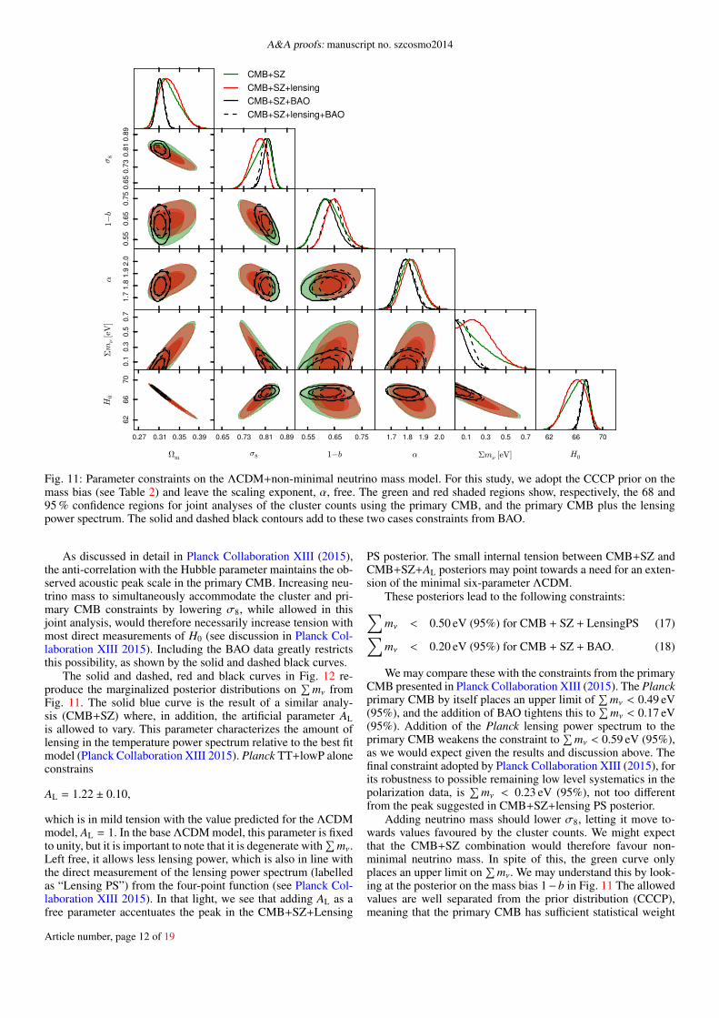
Figure 11 presents a joint analysis of the cluster counts forthe CCCP mass bias prior with primary CMB, the Planck lens-ing power spectrum, and BAO. The results without BAO (greenand red shaded contours) allow relatively large neutrino masses,up to

∑mν ≈ 0.5 eV; and when adding the lensing power spec-

trum, a small, broad peak appears in the posterior distributionjust above

∑mν = 0.2 eV. We also notice some interesting cor-

relations: the amplitude, σ8, anti-correlates with neutrino mass,as does the Hubble parameter, and larger values of α correspondto larger neutrino mass, lower H0, and lower σ8.



0.31 0.35 0.39

CMB+SZCMB+SZ+lensingCMB+SZ+BAOCMB+SZ+lensing+BAO

0.31 0.35 0.39

0.65

0.73

0.81

0.89

σ8

0.65 0.73 0.81 0.89

0.31 0.35 0.39

0.55

0.65

0.75

1−b

0.65 0.73 0.81 0.89 0.55 0.65 0.75

0.31 0.35 0.39

1.7

1.8

1.9

2.0

α

0.65 0.73 0.81 0.89 0.55 0.65 0.75 1.7 1.8 1.9 2.0

0.31 0.35 0.39

0.1

0.3

0.5

0.7

Σmν[e

V]

0.65 0.73 0.81 0.89 0.55 0.65 0.75 1.7 1.8 1.9 2.0 0.1 0.3 0.5 0.7

0.27 0.31 0.35 0.39

Ωm

6266

70

H0

0.65 0.73 0.81 0.89

σ8

0.55 0.65 0.75

1−b

1.7 1.8 1.9 2.0

α

0.1 0.3 0.5 0.7

Σmν [eV]

62 66 70

H0

Fig. 11: Parameter constraints on the ΛCDM+non-minimal neutrino mass model. For this study, we adopt the CCCP prior on themass bias (see Table 2) and leave the scaling exponent, α, free. The green and red shaded regions show, respectively, the 68 and95 % confidence regions for joint analyses of the cluster counts using the primary CMB, and the primary CMB plus the lensingpower spectrum. The solid and dashed black contours add to these two cases constraints from BAO.

As discussed in detail in Planck Collaboration XIII (2015),the anti-correlation with the Hubble parameter maintains the ob-served acoustic peak scale in the primary CMB. Increasing neu-trino mass to simultaneously accommodate the cluster and pri-mary CMB constraints by lowering σ8, while allowed in thisjoint analysis, would therefore necessarily increase tension withmost direct measurements of H0 (see discussion in Planck Col-laboration XIII 2015). Including the BAO data greatly restrictsthis possibility, as shown by the solid and dashed black curves.

The solid and dashed, red and black curves in Fig. 12 re-produce the marginalized posterior distributions on

∑mν from

Fig. 11. The solid blue curve is the result of a similar analy-sis (CMB+SZ) where, in addition, the artificial parameter ALis allowed to vary. This parameter characterizes the amount oflensing in the temperature power spectrum relative to the best fitmodel (Planck Collaboration XIII 2015). Planck TT+lowP aloneconstrains

AL = 1.22 ± 0.10,

which is in mild tension with the value predicted for the ΛCDMmodel, AL = 1. In the base ΛCDM model, this parameter is fixedto unity, but it is important to note that it is degenerate with

∑mν.

Left free, it allows less lensing power, which is also in line withthe direct measurement of the lensing power spectrum (labelledas “Lensing PS”) from the four-point function (see Planck Col-laboration XIII 2015). In that light, we see that adding AL as afree parameter accentuates the peak in the CMB+SZ+Lensing

PS posterior. The small internal tension between CMB+SZ andCMB+SZ+AL posteriors may point towards a need for an exten-sion of the minimal six-parameter ΛCDM.

These posteriors lead to the following constraints:∑mν < 0.50 eV (95%) for CMB + SZ + LensingPS (17)∑mν < 0.20 eV (95%) for CMB + SZ + BAO. (18)

We may compare these with the constraints from the primaryCMB presented in Planck Collaboration XIII (2015). The Planckprimary CMB by itself places an upper limit of

∑mν < 0.49 eV

(95%), and the addition of BAO tightens this to∑

mν < 0.17 eV(95%). Addition of the Planck lensing power spectrum to theprimary CMB weakens the constraint to

∑mν < 0.59 eV (95%),

as we would expect given the results and discussion above. Thefinal constraint adopted by Planck Collaboration XIII (2015), forits robustness to possible remaining low level systematics in thepolarization data, is

∑mν < 0.23 eV (95%), not too different

from the peak suggested in CMB+SZ+lensing PS posterior.Adding neutrino mass should lower σ8, letting it move to-

wards values favoured by the cluster counts. We might expectthat the CMB+SZ combination would therefore favour non-minimal neutrino mass. In spite of this, the green curve onlyplaces an upper limit on

∑mν. We may understand this by look-

ing at the posterior on the mass bias 1− b in Fig. 11 The allowedvalues are well separated from the prior distribution (CCCP),meaning that the primary CMB has sufficient statistical weight



0.0 0.2 0.4 0.6 0.8 1.0Σmν [eV]

0.0

0.2

0.4

0.6

0.8

1.0

Pro

babili

ty d

ensi

ty

CMB+SZαCMB+SZα+Lensing PSCMB+SZα+BAOCMB+SZα+BAO+Lensing PSCMB+SZα+AL

CMB+SZα (proj)

Fig. 12: Constraints on∑

mν from a joint analysis of the clus-ter counts and primary CMB. The solid and dashed, red andblack lines reproduce the marginalized posterior distributionsfrom Fig. 11. The solid blue line is the posterior from a similaranalysis, but marginalized over the additional parameter AL (seetext). If applied to the present Planck cluster cosmology sample,a future mass calibration of 1 − b = 0.78 ± 0.01 would result inthe bold, dotted green posterior curve.

to strongly override the prior. The lensing power spectrum, infavouring slightly lower σ8, reinforces the cluster trend, so thata peak appears in the posterior for

∑mν in the red curve; it is not

enough, however, to bring the posterior on the mass bias in linewith the prior. This indicates that the tension between the clusterand primary CMB constraints is not fully resolved.

One may then ask, how tight must the prior on the mass biasbe to make a difference? To address this question, we performedan analysis assuming a projected tighter prior constraint on themass bias. The informal target precision for cluster mass cali-bration with future large lensing surveys, such as Euclid and theLarge Synoptic Survey Telescope, is 1 %. We therefore considerthe impact of a prior of 1−b = 0.78±0.01 on the present Planckcluster cosmology sample in Figs. 12 and 13.

The latter figure compares the constraints from cluster countsfor this mass bias to the present primary CMB constraints in the(Ωm, σ8)-plane for the base ΛCDM model. The bold, green dot-ted curve in Fig. 12 shows the predicted posterior on the neu-trino mass from a joint analysis of the present Planck clustercounts and primary CMB with this projected mass bias prior.The same prior on a much larger catalogue would demonstrate acorresponding increase in sensitivity to neutrino mass. This sim-ple projection highlights the importance and value of the moreprecise cluster cosmology expected in the future, and it providesclear motivation for further significant effort in mass calibration.This effort will continue with larger samples of clusters withgravitational shear measurements, and also with the new tech-nique of CMB lensing cluster mass measurements.

In general, the mass bias is expected to depend on both massand redshift. A more precise mass calibration study based onmuch larger samples, e.g., Euclid or LSST, would be required todetermine functional forms for the mass bias. A dependence onmass/redshift can be accounted for by appropriate values for α/βin our formalism.

0.28 0.30 0.32 0.34 0.36 0.38 0.40Ωm

0.70

0.75

0.80

0.85

0.90

σ8

CMBCMB+BAOSZα+BAO (proj)

Fig. 13: Prediction of cluster constraints with a possible futuremass bias prior of 1 − b = 0.78 ± 0.01. The black shaded re-gion and dashed contours reproduce the current primary CMBand primary CMB+BAO constraints from Planck for the baseΛCDM model. The red shaded contours present the constraintsexpected from this mass bias prior applied to the present Planckcluster cosmology sample with the SZ+BAO+BBN data set.

8. Summary and discussion

Our 2015 analysis incorporates a number of improvements andnew information relative to our first study in Planck Collabora-tion XX (2014). With more data, we have a larger cluster cos-mology sample, increased by more than a factor of 2, and weimplement a two-dimensional likelihood over the counts in bothredshift and signal-to-noise. We have also performed new testsof the selection function using MCXC and SPT cluster cata-logues as truth tables. The selection function from these exter-nal checks and internal simulations of the Planck catalogue con-struction agree with each other and can be reasonably modelledby a simple analytical expression derived by assuming noise isthe dominant factor (see the Appendix). One possible system-atic effect that warrants further study is IR emission from clustermember galaxies. Finally, we have examined the implications ofthree recent determinations of the cluster mass bias parameter,1 − b. The two-dimensional likelihood with the 2015 catalogueand mass bias priors will be implemented in CosmoMC.

Our analysis confirms the results of the 2013 study. Thecounts are consistent with those of 2013, illustrated by the agree-ment in the constraints on Ωm and σ8 when using the same SZobservable-mass relations (see Fig. 3). The gain in statistical pre-cision is less than expected from the larger catalogue, whichis likely related to the fact that the fit to the redshift distribu-tion with the X-ray prior on α is only marginal. Our new two-dimensional approach yields consistent but more robust con-straints than the one-dimensional likelihood over just the red-shift distribution; it is less sensitive to the slope of the scalingrelation, α, and it provides a better fit to the counts than in theone-dimensional case.

Using the two-dimensional likelihood as our baseline, we ex-tracted new cosmological constraints using three different clus-ter mass scales represented by the mass bias prior distributionsgiven in Table 2. The first two come from galaxy shear obser-vations of samples of Planck clusters. They differ by about 1σ,with the WtG result favouring larger mass bias. We have alsoimplemented a novel method for measuring cluster masses based



on lensing of the CMB temperature anisotropies behind clusters(Melin & Bartlett 2014); it gives a mass bias averaged over theentire cluster cosmology sample, although with larger statisticaluncertainty.

As a new method requiring further exploration, we con-sider CMB lensing less robust at present than galaxy lensingmass measurements, but highly promising. Similar CMB-basedmass measurements have recently been published by SPT (Bax-ter et al. 2014) and ACT (Madhavacheril et al. 2014). The ap-proach is appealing because it is subject to different systematiceffects than gravitational shear and because it can be applied tolarge cluster samples, thanks to the extensive sky coverage ofthe CMB experiments, with Planck of course covering the entiresky. Gravitational shear surveys will attain large sky coverage inthe near future with the Dark Energy Survey (DES), and in themore distant future with the Euclid and WFIRST space missionsand the Large Synoptic Survey Telescope.

Our central result from analysis of the 2015 Planck clustercounts is shown in Fig. 7. Depending on the mass bias prior,we find varying degrees of tension with the primary CMB re-sults, as in 2013. The mass bias required to bring the clustercounts and CMB into full agreement is larger than indicated byany of the three priors and corresponds to 1 − b = 0.58 ± 0.04.Fig. 8 illustrates the situation. The WtG prior almost eliminatesthe tension, but not quite, while both the CCCP and CMB lens-ing priors remain in noticeable disagreement. Our largest sourceof modelling uncertain is, as in 2013, the mass bias.

Tension between low redshift determinations of σ8 and thePlanck primary CMB results are not unique to the Planck clus-ter counts. Among SZ cluster surveys, both SPT and ACT arein broad agreement with our findings, the latter depending onwhich SZ-mass scaling relation is used, as detailed in our 2013analysis (Planck Collaboration XX 2014). Furthermore the newSPT cosmological analysis (Bocquet et al. 2014) shows a sig-nificant shift between the cluster mass scale determined fromthe velocity dispersion or YX and what is needed to satisfyPlanck or WMAP9 CMB constraints (e.g., figure 2 Bocquet et al.2014). In a study of the REFLEX X-ray luminosity function,Böhringer et al. (2014) also report general agreement with ourcluster findings. On the other hand, Mantz et al. (2014) find thattheir X-ray cluster counts, when using the WtG mass calibra-tion, match the primary CMB constraints. Angrick et al. (2015)also find good agreement with the primary CMB constraints, fit-ting their X-ray temperature function with results from hydrody-namical simulations, and Simet et al. (2015) recently measured< MX/MWL >= 0.66+0.07

−0.12 for the RBC X-ray galaxy cluster cat-alogue.

The situation is thus not yet satisfactory. It is unclear if thesemodest tensions arise from low-level systematics in the astro-physical studies, or are the first glimpse of something more im-portant. The most obvious extension to the base ΛCDM modelthat could in principle reconcile the differences is a non-minimalsum of neutrino masses. This, unfortunately, does not providesuch a straightforward solution. While it is true that adding neu-trino mass does lower σ8 relative to the base ΛCDM predictionfrom the primary CMB, it does so at the the cost of increas-ing tension in other parameters; for example, it lowers Planck’svalue for the Hubble constant which is already lower than manydirect estimates.

Figure 14 highlights these points by showing constraints inthe (Ωm, σ8)- and (H0, σ8)-planes for the CCCP mass bias pa-rameter. Adding variable neutrino mass relaxes constraints fromthe primary CMB (shaded contours) towards lower σ8, but while

0.20 0.25 0.30 0.35 0.40Ωm

0.62

0.67

0.72

0.77

0.82

0.87

σ8

+∑

mν

SZ+BAO CMB +lensing+BAO ΛCDM

60 65 70 75H0

+∑

mν

Fig. 14: Effects of neutrino mass. The open solid magenta con-tours reproduce our cluster constraints when marginalizing overvariable neutrino mass. The violet shaded contours trace the con-straints on the base ΛCDM model (with fixed neutrino mass),while the other shaded regions give constraints from the primaryCMB only or combined with lensing and BAO when addingand marginalizing over variable neutrino mass. In this figure,the CMB likelihood is based on Planck TT, TE, EE+lowP whileonly Planck TT+lowP is used in the equivalent figure in PlanckCollaboration XIII (2015).

simultaneously increasing Ωm and decreasing H0. And the ten-sion remains pronounced, regardless of the neutrino mass.

Another possibility is that baryonic physics influences thelate-time evolution of the density perturbations. Strong feedbackfrom active galactic nuclei (van Daalen et al. 2011; Martizzi et al.2014) can potentially damp growth and lower σ8 through expul-sion of matter from dark matter halos. This same effect couldalso reduce the mass of cluster halos and hence the predictionfor their abundance, which is based on dark matter only simula-tions (Cui et al. 2014; Velliscig et al. 2014; Bocquet et al. 2015).It does not appear, however, that these effects are sufficientlylarge to explain the tension between low redshift and primaryCMB constraints hinted at by the different observations (e.g.,Cusworth et al. 2014; Costanzi et al. 2014). In addition, the vi-olent feedback necessary for important impact might be difficultto reconcile with observations of the baryon content of dark mat-ter halos (e.g., Planck Collaboration Int. XI 2013; Greco et al.2015), altough this point is still under discussion (e.g., Planelleset al. 2014).

In conclusion, we return to the main uncertainty in interpre-tation of the cluster counts, namely the mass bias. It could beargued that the current accuracy is at the level of 10 - 15 %,based on the difference between different analyses and some-what larger than their quoted statistical uncertainties. Progresswill certainly follow with improvement in these measurements.We illustrate the potential impact of a 1% determination of themass bias in Figs. 12 and 13. Such a result would, depending onthe central value, significantly clarify the extent of any tensionsand possible necessity for extensions to the base ΛCDM model.This precision is the avowed target of the large lensing surveys,such as Euclid, WFIRST, and LSST. In the shorter term, we mayexpect valuable movement in this direction from DES and CMBlensing cluster mass measurements.Acknowledgements. The Planck Collaboration acknowledges the support of:ESA; CNES, and CNRS/INSU-IN2P3-INP (France); ASI, CNR, and INAF(Italy); NASA and DoE (USA); STFC and UKSA (UK); CSIC, MINECO, JAand RES (Spain); Tekes, AoF, and CSC (Finland); DLR and MPG (Germany);CSA (Canada); DTU Space (Denmark); SER/SSO (Switzerland); RCN (Nor-way); SFI (Ireland); FCT/MCTES (Portugal); ERC and PRACE (EU). A de-scription of the Planck Collaboration and a list of its members, indicating which



technical or scientific activities they have been involved in, can be found athttp://www.cosmos.esa.int/web/planck/planck-collaboration.

ReferencesAnderson, L., Aubourg, É., Bailey, S., et al. 2014, MNRAS, 441, 24Anderson, L., Aubourg, E., Bailey, S., et al. 2012, MNRAS, 427, 3435Andreon, S. 2014, A&A, 570, L10Angrick, C., Pace, F., Bartelmann, M., & Roncarelli, M. 2015, ArXiv e-printsAngulo, R. E., Springel, V., White, S. D. M., et al. 2012, MNRAS, 426, 2046Arnaud, M., Pratt, G. W., Piffaretti, R., et al. 2010, A&A, 517, A92Arnaud et al., i. p. 2015Battye, R. A., Charnock, T., & Moss, A. 2014, ArXiv e-printsBaxter, E. J., Keisler, R., Dodelson, S., et al. 2014, ArXiv e-printsBecker, M. R. & Kravtsov, A. V. 2011, ApJ, 740, 25Benson, B. A., de Haan, T., Dudley, J. P., et al. 2013, ApJ, 763, 147Bersanelli, M., Mandolesi, N., Butler, R. C., et al. 2010, A&A, 520, A4Betoule, M., Kessler, R., Guy, J., et al. 2014, A&A, 568, A22Beutler, F., Blake, C., Colless, M., et al. 2011, MNRAS, 416, 3017Bleem, L. E., Stalder, B., de Haan, T., et al. 2014, ArXiv e-printsBocquet, S., Saro, A., Dolag, K., & Mohr, J. J. 2015, ArXiv e-printsBocquet, S., Saro, A., Mohr, J. J., et al. 2014, ArXiv e-printsBöhringer, H., Chon, G., & Collins, C. A. 2014, A&A, 570, A31Carlstrom, J. E., Ade, P. A. R., Aird, K. A., et al. 2011, PASP, 123, 568Carvalho, P., Rocha, G., & Hobson, M. P. 2009, MNRAS, 393, 681Chamballu, A., Bartlett, J. G., & Melin, J.-B. 2012, A&A, 544, A40Costanzi, M., Sartoris, B., Viel, M., & Borgani, S. 2014, J. Cosmology Astropart.

Phys., 10, 81Cui, W., Borgani, S., & Murante, G. 2014, MNRAS, 441, 1769Cusworth, S. J., Kay, S. T., Battye, R. A., & Thomas, P. A. 2014, MNRAS, 439,

2485Greco, J. P., Hill, J. C., Spergel, D. N., & Battaglia, N. 2015, ApJ, 808, 151Hasselfield, M., Hilton, M., Marriage, T. A., et al. 2013, J. Cosmology Astropart.

Phys., 7, 8Hoekstra, H., Herbonnet, R., Muzzin, A., et al. 2015, MNRAS, 449, 685Hu, W. & Kravtsov, A. V. 2003, ApJ, 584, 702Lamarre, J., Puget, J., Ade, P. A. R., et al. 2010, A&A, 520, A9Lewis, A. & Challinor, A. 2006, Phys. Rep., 429, 1Madhavacheril, M., Sehgal, N., Allison, R., et al. 2014, ArXiv e-printsMantz, A. B., von der Linden, A., Allen, S. W., et al. 2014, ArXiv e-printsMarrone, D. P., Smith, G. P., Okabe, N., et al. 2012, ApJ, 754, 119Martizzi, D., Mohammed, I., Teyssier, R., & Moore, B. 2014, MNRAS, 440,

2290Melin, J., Bartlett, J. G., & Delabrouille, J. 2006, A&A, 459, 341Melin, J.-B. & Bartlett, J. G. 2014, ArXiv e-printsMeneghetti, M., Rasia, E., Merten, J., et al. 2010, A&A, 514, A93Mennella, A., Butler, R. C., Curto, A., et al. 2011, A&A, 536, A3Merten, J., Meneghetti, M., Postman, M., et al. 2014, ArXiv e-printsNagai, D., Kravtsov, A. V., & Vikhlinin, A. 2007, ApJ, 668, 1Navarro, J. F., Frenk, C. S., & White, S. D. M. 1997, ApJ, 490, 493Olive, K. A. 2013, in American Institute of Physics Conference Series, Vol. 1548,

American Institute of Physics Conference Series, ed. L. A. Uren˜a-López,R. Becerril-Bárcenas, & R. Linares-Romero, 116–125

Padmanabhan, N., Xu, X., Eisenstein, D. J., et al. 2012, MNRAS, 427, 2132Piffaretti, R., Arnaud, M., Pratt, G. W., Pointecouteau, E., & Melin, J.-B. 2011,

A&A, 534, A109Piffaretti, R. & Valdarnini, R. 2008, A&A, 491, 71Planck HFI Core Team. 2011, A&A, 536, A4Planck Collaboration I. 2011, A&A, 536, A1Planck Collaboration I. 2014, A&A, 571, A1Planck Collaboration XVI. 2014, A&A, 571, A16Planck Collaboration XX. 2014, A&A, 571, A20Planck Collaboration XXIX. 2014, A&A, 571, A29Planck Collaboration I. 2015, A&A, submittedPlanck Collaboration II. 2015, A&A, submittedPlanck Collaboration III. 2015, A&A, submittedPlanck Collaboration IV. 2015, A&A, submittedPlanck Collaboration V. 2015, A&A, submittedPlanck Collaboration VI. 2015, A&A, submittedPlanck Collaboration VII. 2015, A&A, submittedPlanck Collaboration VIII. 2015, A&A, submittedPlanck Collaboration IX. 2015, A&A, submittedPlanck Collaboration X. 2015, A&A, submittedPlanck Collaboration XI. 2015, A&A, submittedPlanck Collaboration XII. 2015, in preparationPlanck Collaboration XIII. 2015, A&A, submittedPlanck Collaboration XIV. 2015, A&A, submittedPlanck Collaboration XV. 2015, A&A, submitted

Planck Collaboration XVI. 2015, A&A, submittedPlanck Collaboration XVII. 2015, A&A, submittedPlanck Collaboration XVIII. 2015, A&A, submittedPlanck Collaboration XIX. 2015, A&A, submittedPlanck Collaboration XX. 2015, A&A, submittedPlanck Collaboration XXI. 2015, A&A, submittedPlanck Collaboration XXII. 2015, A&A, submittedPlanck Collaboration XXIII. 2015, in preparationPlanck Collaboration XXIV. 2015, A&A, submittedPlanck Collaboration XXV. 2015, A&A, submittedPlanck Collaboration XXVI. 2015, A&A, submittedPlanck Collaboration XXVII. 2015, A&A, submittedPlanck Collaboration XXVIII. 2015, A&A, submittedPlanck Collaboration Int. III. 2013, A&A, 550, A129Planck Collaboration Int. XI. 2013, A&A, 557, A52Planelles, S., Borgani, S., Fabjan, D., et al. 2014, MNRAS, 438, 195Postman, M., Coe, D., Benítez, N., et al. 2012, ApJS, 199, 25Rasia, E., Ettori, S., Moscardini, L., et al. 2006, MNRAS, 369, 2013Rasia, E., Lau, E. T., Borgani, S., et al. 2014, ApJ, 791, 96Rasia, E., Meneghetti, M., Martino, R., et al. 2012, New Journal of Physics, 14,

055018Reichardt, C. L., Stalder, B., Bleem, L. E., et al. 2013, ApJ, 763, 127Riess, A. G., Macri, L., Casertano, S., et al. 2011, ApJ, 730, 119Rozo, E., Bartlett, J. G., Evrard, A. E., & Rykoff, E. S. 2014a, MNRAS, 438, 78Rozo, E., Evrard, A. E., Rykoff, E. S., & Bartlett, J. G. 2014b, MNRAS, 438, 62Rozo, E., Rykoff, E. S., Bartlett, J. G., & Evrard, A. 2014c, MNRAS, 438, 49Simet, M., Battaglia, N., Mandelbaum, R., & Seljak, U. 2015, ArXiv e-printsSteigman, G. 2008, ArXiv e-printsSwetz, D. S., Ade, P. A. R., Amiri, M., et al. 2011, ApJS, 194, 41Tauber, J. A., Mandolesi, N., Puget, J., et al. 2010, A&A, 520, A1Tinker, J., Kravtsov, A. V., Klypin, A., et al. 2008, ApJ, 688, 709Umetsu, K., Medezinski, E., Nonino, M., et al. 2014, ArXiv e-printsvan Daalen, M. P., Schaye, J., Booth, C. M., & Dalla Vecchia, C. 2011, MNRAS,

415, 3649Velliscig, M., van Daalen, M. P., Schaye, J., et al. 2014, MNRAS, 442, 2641von der Linden, A., Allen, M. T., Applegate, D. E., et al. 2014a, MNRAS, 439, 2von der Linden, A., Mantz, A., Allen, S. W., et al. 2014b, ArXiv e-printsWatson, W. A., Iliev, I. T., D’Aloisio, A., et al. 2013a, MNRAS, 433, 1230Watson, W. A., Iliev, I. T., D’Aloisio, A., et al. 2013b, arXiv:1212.0095v1Zaldarriaga, M. & Seljak, U. 1999, Phys. Rev. D, 59, 123507

1 APC, AstroParticule et Cosmologie, Université Paris Diderot,CNRS/IN2P3, CEA/lrfu, Observatoire de Paris, Sorbonne ParisCité, 10, rue Alice Domon et Léonie Duquet, 75205 Paris Cedex13, France

2 Aalto University Metsähovi Radio Observatory and Dept of RadioScience and Engineering, P.O. Box 13000, FI-00076 AALTO, Fin-land

3 African Institute for Mathematical Sciences, 6-8 Melrose Road,Muizenberg, Cape Town, South Africa

4 Agenzia Spaziale Italiana Science Data Center, Via del Politecnicosnc, 00133, Roma, Italy

5 Aix Marseille Université, CNRS, LAM (Laboratoired’Astrophysique de Marseille) UMR 7326, 13388, Marseille,France

6 Astrophysics Group, Cavendish Laboratory, University of Cam-bridge, J J Thomson Avenue, Cambridge CB3 0HE, U.K.

7 Astrophysics & Cosmology Research Unit, School of Mathe-matics, Statistics & Computer Science, University of KwaZulu-Natal, Westville Campus, Private Bag X54001, Durban 4000, SouthAfrica

8 Atacama Large Millimeter/submillimeter Array, ALMA SantiagoCentral Offices, Alonso de Cordova 3107, Vitacura, Casilla 7630355, Santiago, Chile

9 CGEE, SCS Qd 9, Lote C, Torre C, 4 andar, Ed. Parque CidadeCorporate, CEP 70308-200, Brasília, DF, Brazil

10 CITA, University of Toronto, 60 St. George St., Toronto, ON M5S3H8, Canada

11 CNRS, IRAP, 9 Av. colonel Roche, BP 44346, F-31028 Toulousecedex 4, France

12 CRANN, Trinity College, Dublin, Ireland13 California Institute of Technology, Pasadena, California, U.S.A.14 Centre for Theoretical Cosmology, DAMTP, University of Cam-

bridge, Wilberforce Road, Cambridge CB3 0WA, U.K.


http://www.cosmos.esa.int/web/planck/planck-collaboration


15 Centro de Estudios de Física del Cosmos de Aragón (CEFCA),Plaza San Juan, 1, planta 2, E-44001, Teruel, Spain

16 Computational Cosmology Center, Lawrence Berkeley NationalLaboratory, Berkeley, California, U.S.A.

17 Consejo Superior de Investigaciones Científicas (CSIC), Madrid,Spain

18 DSM/Irfu/SPP, CEA-Saclay, F-91191 Gif-sur-Yvette Cedex,France

19 DTU Space, National Space Institute, Technical University of Den-mark, Elektrovej 327, DK-2800 Kgs. Lyngby, Denmark

20 Département de Physique Théorique, Université de Genève, 24,Quai E. Ansermet,1211 Genève 4, Switzerland

21 Departamento de Astrofísica, Universidad de La Laguna (ULL),E-38206 La Laguna, Tenerife, Spain

22 Departamento de Física, Universidad de Oviedo, Avda. CalvoSotelo s/n, Oviedo, Spain

23 Department of Astronomy and Astrophysics, University ofToronto, 50 Saint George Street, Toronto, Ontario, Canada

24 Department of Astrophysics/IMAPP, Radboud University Ni-jmegen, P.O. Box 9010, 6500 GL Nijmegen, The Netherlands

25 Department of Physics & Astronomy, University of BritishColumbia, 6224 Agricultural Road, Vancouver, British Columbia,Canada

26 Department of Physics and Astronomy, Dana and David DornsifeCollege of Letter, Arts and Sciences, University of Southern Cali-fornia, Los Angeles, CA 90089, U.S.A.

27 Department of Physics and Astronomy, University College Lon-don, London WC1E 6BT, U.K.

28 Department of Physics, Florida State University, Keen PhysicsBuilding, 77 Chieftan Way, Tallahassee, Florida, U.S.A.

29 Department of Physics, Gustaf Hällströmin katu 2a, University ofHelsinki, Helsinki, Finland

30 Department of Physics, Princeton University, Princeton, New Jer-sey, U.S.A.

31 Department of Physics, University of California, Santa Barbara,California, U.S.A.

32 Department of Physics, University of Illinois at Urbana-Champaign, 1110 West Green Street, Urbana, Illinois, U.S.A.

33 Dipartimento di Fisica e Astronomia G. Galilei, Università degliStudi di Padova, via Marzolo 8, 35131 Padova, Italy

34 Dipartimento di Fisica e Scienze della Terra, Università di Ferrara,Via Saragat 1, 44122 Ferrara, Italy

35 Dipartimento di Fisica, Università La Sapienza, P. le A. Moro 2,Roma, Italy

36 Dipartimento di Fisica, Università degli Studi di Milano, Via Celo-ria, 16, Milano, Italy

37 Dipartimento di Fisica, Università degli Studi di Trieste, via A. Va-lerio 2, Trieste, Italy

38 Dipartimento di Matematica, Università di Roma Tor Vergata, Viadella Ricerca Scientifica, 1, Roma, Italy

39 Discovery Center, Niels Bohr Institute, Blegdamsvej 17, Copen-hagen, Denmark

40 Discovery Center, Niels Bohr Institute, Copenhagen University,Blegdamsvej 17, Copenhagen, Denmark

41 European Southern Observatory, ESO Vitacura, Alonso de Cordova3107, Vitacura, Casilla 19001, Santiago, Chile

42 European Space Agency, ESAC, Planck Science Office, Caminobajo del Castillo, s/n, Urbanización Villafranca del Castillo, Vil-lanueva de la Cañada, Madrid, Spain

43 European Space Agency, ESTEC, Keplerlaan 1, 2201 AZ Noord-wijk, The Netherlands

44 Gran Sasso Science Institute, INFN, viale F. Crispi 7, 67100L’Aquila, Italy

45 HGSFP and University of Heidelberg, Theoretical Physics Depart-ment, Philosophenweg 16, 69120, Heidelberg, Germany

46 Haverford College Astronomy Department, 370 Lancaster Avenue,Haverford, Pennsylvania, U.S.A.

47 Helsinki Institute of Physics, Gustaf Hällströmin katu 2, Universityof Helsinki, Helsinki, Finland

48 INAF - Osservatorio Astrofisico di Catania, Via S. Sofia 78, Cata-nia, Italy

49 INAF - Osservatorio Astronomico di Padova, Vicolodell’Osservatorio 5, Padova, Italy

50 INAF - Osservatorio Astronomico di Roma, via di Frascati 33,Monte Porzio Catone, Italy

51 INAF - Osservatorio Astronomico di Trieste, Via G.B. Tiepolo 11,Trieste, Italy

52 INAF/IASF Bologna, Via Gobetti 101, Bologna, Italy53 INAF/IASF Milano, Via E. Bassini 15, Milano, Italy54 INFN, Sezione di Bologna, Via Irnerio 46, I-40126, Bologna, Italy55 INFN, Sezione di Roma 1, Università di Roma Sapienza, Piazzale

Aldo Moro 2, 00185, Roma, Italy56 INFN, Sezione di Roma 2, Università di Roma Tor Vergata, Via

della Ricerca Scientifica, 1, Roma, Italy57 INFN/National Institute for Nuclear Physics, Via Valerio 2, I-34127

Trieste, Italy58 IPAG: Institut de Planétologie et d’Astrophysique de Grenoble,

Université Grenoble Alpes, IPAG, F-38000 Grenoble, France,CNRS, IPAG, F-38000 Grenoble, France

59 ISDC, Department of Astronomy, University of Geneva, ch.d’Ecogia 16, 1290 Versoix, Switzerland

60 IUCAA, Post Bag 4, Ganeshkhind, Pune University Campus, Pune411 007, India

61 Imperial College London, Astrophysics group, Blackett Labora-tory, Prince Consort Road, London, SW7 2AZ, U.K.

62 Infrared Processing and Analysis Center, California Institute ofTechnology, Pasadena, CA 91125, U.S.A.

63 Institut Néel, CNRS, Université Joseph Fourier Grenoble I, 25 ruedes Martyrs, Grenoble, France

64 Institut Universitaire de France, 103, bd Saint-Michel, 75005, Paris,France

65 Institut d’Astrophysique Spatiale, CNRS, Univ. Paris-Sud, Univer-sité Paris-Saclay, Bât. 121, 91405 Orsay cedex, France

66 Institut d’Astrophysique de Paris, CNRS (UMR7095), 98 bisBoulevard Arago, F-75014, Paris, France

67 Institut für Theoretische Teilchenphysik und Kosmologie, RWTHAachen University, D-52056 Aachen, Germany

68 Institute for Space Sciences, Bucharest-Magurale, Romania69 Institute of Astronomy, University of Cambridge, Madingley Road,

Cambridge CB3 0HA, U.K.70 Institute of Theoretical Astrophysics, University of Oslo, Blindern,

Oslo, Norway71 Instituto de Astrofísica de Canarias, C/Vía Láctea s/n, La Laguna,

Tenerife, Spain72 Instituto de Física de Cantabria (CSIC-Universidad de Cantabria),

Avda. de los Castros s/n, Santander, Spain73 Istituto Nazionale di Fisica Nucleare, Sezione di Padova, via Mar-

zolo 8, I-35131 Padova, Italy74 Jet Propulsion Laboratory, California Institute of Technology, 4800

Oak Grove Drive, Pasadena, California, U.S.A.75 Jodrell Bank Centre for Astrophysics, Alan Turing Building,

School of Physics and Astronomy, The University of Manchester,Oxford Road, Manchester, M13 9PL, U.K.

76 Kavli Institute for Cosmological Physics, University of Chicago,Chicago, IL 60637, USA

77 Kavli Institute for Cosmology Cambridge, Madingley Road, Cam-bridge, CB3 0HA, U.K.

78 Kazan Federal University, 18 Kremlyovskaya St., Kazan, 420008,Russia

79 LAL, Université Paris-Sud, CNRS/IN2P3, Orsay, France80 LERMA, CNRS, Observatoire de Paris, 61 Avenue de

l’Observatoire, Paris, France81 Laboratoire AIM, IRFU/Service d’Astrophysique - CEA/DSM -

CNRS - Université Paris Diderot, Bât. 709, CEA-Saclay, F-91191Gif-sur-Yvette Cedex, France

82 Laboratoire Traitement et Communication de l’Information, CNRS(UMR 5141) and Télécom ParisTech, 46 rue Barrault F-75634Paris Cedex 13, France



83 Laboratoire de Physique Subatomique et Cosmologie, UniversitéGrenoble-Alpes, CNRS/IN2P3, 53, rue des Martyrs, 38026 Greno-ble Cedex, France

84 Laboratoire de Physique Théorique, Université Paris-Sud 11 &CNRS, Bâtiment 210, 91405 Orsay, France

85 Lawrence Berkeley National Laboratory, Berkeley, California,U.S.A.

86 Lebedev Physical Institute of the Russian Academy of Sciences,Astro Space Centre, 84/32 Profsoyuznaya st., Moscow, GSP-7,117997, Russia

87 Max-Planck-Institut für Astrophysik, Karl-Schwarzschild-Str. 1,85741 Garching, Germany

88 McGill Physics, Ernest Rutherford Physics Building, McGill Uni-versity, 3600 rue University, Montréal, QC, H3A 2T8, Canada

89 National University of Ireland, Department of ExperimentalPhysics, Maynooth, Co. Kildare, Ireland

90 Nicolaus Copernicus Astronomical Center, Bartycka 18, 00-716Warsaw, Poland

91 Niels Bohr Institute, Blegdamsvej 17, Copenhagen, Denmark92 Niels Bohr Institute, Copenhagen University, Blegdamsvej 17,

Copenhagen, Denmark93 Nordita (Nordic Institute for Theoretical Physics), Roslagstulls-

backen 23, SE-106 91 Stockholm, Sweden94 Optical Science Laboratory, University College London, Gower

Street, London, U.K.95 SISSA, Astrophysics Sector, via Bonomea 265, 34136, Trieste,

Italy96 SMARTEST Research Centre, Università degli Studi e-Campus,

Via Isimbardi 10, Novedrate (CO), 22060, Italy97 School of Physics and Astronomy, Cardiff University, Queens

Buildings, The Parade, Cardiff, CF24 3AA, U.K.98 School of Physics and Astronomy, University of Nottingham, Not-

tingham NG7 2RD, U.K.99 Sorbonne Université-UPMC, UMR7095, Institut d’Astrophysique

de Paris, 98 bis Boulevard Arago, F-75014, Paris, France100 Space Research Institute (IKI), Russian Academy of Sciences,

Profsoyuznaya Str, 84/32, Moscow, 117997, Russia101 Space Sciences Laboratory, University of California, Berkeley, Cal-

ifornia, U.S.A.102 Special Astrophysical Observatory, Russian Academy of Sciences,

Nizhnij Arkhyz, Zelenchukskiy region, Karachai-Cherkessian Re-public, 369167, Russia

103 Stanford University, Dept of Physics, Varian Physics Bldg, 382 ViaPueblo Mall, Stanford, California, U.S.A.

104 Sub-Department of Astrophysics, University of Oxford, KebleRoad, Oxford OX1 3RH, U.K.

105 The Oskar Klein Centre for Cosmoparticle Physics, Department ofPhysics,Stockholm University, AlbaNova, SE-106 91 Stockholm,Sweden

106 Theory Division, PH-TH, CERN, CH-1211, Geneva 23, Switzer-land

107 UPMC Univ Paris 06, UMR7095, 98 bis Boulevard Arago, F-75014, Paris, France

108 Université de Toulouse, UPS-OMP, IRAP, F-31028 Toulouse cedex4, France

109 University Observatory, Ludwig Maximilian University of Munich,Scheinerstrasse 1, 81679 Munich, Germany

110 University of Granada, Departamento de Física Teórica y del Cos-mos, Facultad de Ciencias, Granada, Spain

111 University of Granada, Instituto Carlos I de Física Teórica y Com-putacional, Granada, Spain

112 Warsaw University Observatory, Aleje Ujazdowskie 4, 00-478Warszawa, Poland

Appendix A: Modelling uncertainties

We examine the robustness of our cosmological constraints tomodelling uncertainties. We first consider sensitivity to the cos-mological sample and to our modelling of the completeness

0.25 0.30 0.35 0.40Ωm

0.70

0.72

0.74

0.76

0.78

0.80

σ8

MMF3 ERFMMF3 QAINTER QA

Fig. A.1: Robustness to the choice of cluster sample and selec-tion function model. The shaded contours give the cosmologicalconstraints from the 2015 MMF3 cluster catalogue using the an-alytical (error function, ERF) selection function model (grey),the MMF3 Monte Carlo selection function (red), and the MonteCarlo selection function for the intersection sample (blue). Ourfinal constraints are obtained from the MMF3 ERF model. Forthis comparison, we adopt the SZ+BAO+BBN data set and wefix 1 − b = 0.8.

function in Sect. A.1, and then look at the effect of using a dif-ferent mass function in Sec. A.2. In Sec. A.3, we show that ourconstraints are robust against redshift evolution of the scalingrelations.

Appendix A.1: Choice of the sample and selection function

For our baseline analysis, we use the MMF3 cosmological sam-ple and its associated completeness based on the analyticalapproximation using the error function (Eq. 14). In Fig. A.1we show how the Monte Carlo determined selection functionchanges the cosmological constraints (labelled QA for “QualityAssessment” in the figure). We also present the constraints ob-tained from the intersection sample defined in Sec. 2. The figureis based on the 1D N(z) likelihood, for which the Monte Carlocompleteness can be easily computed, and we use the baselineSZ+BAO+BBN data set and fix 1 − b = 0.8. The MMF3 ERFcontour is thus close to the q = 6 contour of Fig. 3, the onlydifference being that σln Y is fixed to zero in Fig. A.1. while it isconstrained by the Table 1 prior in Fig. 3. The impact of adoptingthe intersection sample and/or the QA completeness function issmall (< 0.5σ) for both Ωm and σ8.

Appendix A.2: Mass function

We use the Tinker et al. (2008) mass function for our baselineanalysis. To characterize the influence of this choice, we exam-ine constraints when adopting the mass function from Watsonet al. (2013a) instead. We employ our two-dimensional N(z, q)likelihood (with the CCCP mass bias prior and α constrained)and combine with BAO and BBN prior constraints, showing theresult in Fig. A.2. The Tinker et al. contour of Fig. A.2 is thusidentical to the N(z, q) contour with α constrained, as given inFig. 5. The new mass function shifts our constraints by about1σ towards higher Ωm and lower σ8, along the main degeneracyline, hence increasing the tension with the Planck primary CMB



0.25 0.30 0.35 0.40 0.45Ωm

0.65

0.70

0.75

0.80

0.85

σ8

Tinker et al.Watson et al.

Fig. A.2: Robustness to the choice of mass function. The greyshaded contours give the cosmological constraints when usingthe Tinker et al. (2008) mass function, corresponding to our fi-nal result. This is compared to constraints obtained when usingthe Watson et al. (2013a) mass function, shown as the red shadedcontours. In this figure we adopt the SZ+BAO+BBN data set andthe CCCP mass bias prior.

constraints. We note that we use the general fit from Eq. (12)of Watson et al. (2013a) (independent of redshift). This was notthe case for our 2013 paper (Planck Collaboration XX 2014)where we adopted the AHF fit with parameters varying with red-shift in the first posted version of the paper (see Watson et al.2013b, on ArXiv.org), which was subsequently found to be in-correct.

Appendix A.3: Redshift evolution of the Y-M relation

Throughout our baseline analysis, we fix the redshift evolutionexponent β = 0.66 (self-similar prediction) in Eq. (7). Here weexamine the impact of allowing this parameter to vary. Con-straints when leaving β free are shown in Fig. A.3. The “β fixed,α constrained” case corresponds to the two-dimensional N(z, q)likelihood (CCCP mass bias prior and α constrained) combinedwith BAO and BBN, as in Fig. A.2. This contour is also identicalto the N(z, q) contour with α constrained, shown in Fig. 5. Forthe “β constrained” cases, β is allowed to vary over the range0.66 ± 0.50 (Table 1). This increases the size of our constraintsalong the major degeneracy between Ωm and σ8, but does notbring them into any closer agreement with the primary CMB.

Andreon (2014) recently reanalyzed the subsample of 71clusters used in Planck Collaboration XX (2014). Through ajoint fit to the normalization and redshift evolution of the Y-M re-lation, he found a significant detection of non-standard redshiftevolution. It is possible that this conclusion is driven by sys-tematic effects in the X-ray and SZ measurements. In particular,low-z objects have larger angular sizes, and so measurement oftheir X-ray and SZ quantities are subject to different systematiceffects compared to equivalent measurements for high-z objects.Appendix D of Planck Collaboration XXIX (2014) includes acomprehensive discussion of the various systematic effects thatmay have an impact on measurement of the Y-M relation. Giventhese caveats, we believe that it is premature to draw definitiveconclusions on the evolution of the Y-M relation.

0.25 0.30 0.35 0.40 0.45Ωm

0.62

0.70

0.78

0.86

0.94

σ8

β fixed, α constrained

β constrained, α constrained

β constrained, α free

Fig. A.3: Robustness to redshift evolution in the SZ-mass scal-ing relation. The different contours show the constraints whenrelaxing the redshift evolution exponent, β, of Eq. (7). The blackcontours result from fixing β = 0.66, our fiducial value through-out, with α constrained by the Gaussian X-ray prior of Table 1.Applying a Gaussian the prior on β instead, from Table 1, pro-duces the blue contours, while the red contours result when wealso leave α free. In this figure we adopt the SZ+BAO+BBNdata set and the CCCP mass bias prior.

Appendix A.4: Slope of the Y − M relation

The one-dimensional analysis of the redshift distribution inSect. 6.2 preferred steeper values of the Y −M scaling exponent,α, than indicated by X-ray studies of local clusters (see Fig. 5,case α free, black contours and curves). This seems to be relatedto the flattening in the redshift distribution around z = 0.2 seen inFigures 4 and 6. To explore this, we separately extracted param-eter constraints from low (z < 0.2) and high (z > 0.2) redshiftbin sets (two and eight bins, respectively) when leaving α free.

Figure A.4 compares the constraints from these splits tothose from the full bin set (with α free). Neither the low northe high redshift bin set on its own prefers the steep slope – theposteriors peak near the X-ray value, i.e, the clusters in each sub-sample follow the expected scaling relation. Cosmological con-straints from the low-z data broaden compared to the full dataset, and bimodality appears in the distribution for Ωm. The high-z data, on the other hand, loose precision on α, although the peakin the posterior shifts to the X-ray value, but maintain constraintson the cosmological parameters that are similar to those from thefull data set.

Only the combined data covering the full redshift range pre-fer the steep slope. The parameters are coupled in a subtle inter-play that favours high values of α and moves the cosmologicalparameters along the degeneracy ridges to settle on their high-zvalues. These degeneracies mask the interplay and unfortunatelymake further exploration difficult with the present data set.



0.25 0.31 0.38 0.44

N(z) α free low-z binsN(z) α free high-z binsN(z) α free all bins

0.25 0.31 0.38 0.44

1.7

2.1

2.5

α

1.7 2.1 2.5

0.25 0.31 0.38 0.44

0.65

0.75

0.85

σ8

1.7 2.1 2.5 0.65 0.75 0.85

0.25 0.31 0.38 0.44Ωm

6267

7277

H0

1.7 2.1 2.5α

0.65 0.75 0.85σ8

62 67 72 77H0

Fig. A.4: Comparison of constraints from the full redshift dis-tribution (in black) to those from the redshift split: two bins atz < 0.2 (in purple) and eight bins at z > 0.2 (in blue). The con-straints are obtained with the one-dimensional likelihood whenleaving α free, and the black curves and contours reproducethose from Fig. 5.


Planck 2015 results. XXIV. Cosmology from Sunyaev ...

Documents

Transcript of Planck 2015 results. XXIV. Cosmology from Sunyaev ...