Plan Bouquets: A Fragrant Approach to Robust Query Processing Jayant R. Haritsa Database Systems Lab...

Plan Bouquets: A Fragrant Approach to Robust Query Processing

Jayant R. HaritsaDatabase Systems Lab

Indian Institute of Science, Bangalore

Plan 1 Plan 2

Plan 5

Plan 4

Plan 3

Dec 2014 1CMG Keynote

Talk Theme Declarative query processing with performance

guarantees has been a highly desirable but equally elusive goal for the database community over the last three decades. I will present a conceptually new approach, called “plan bouquets”, to address this classical problem.

(Joint work with Anshuman Dutt, IISc PhD student)


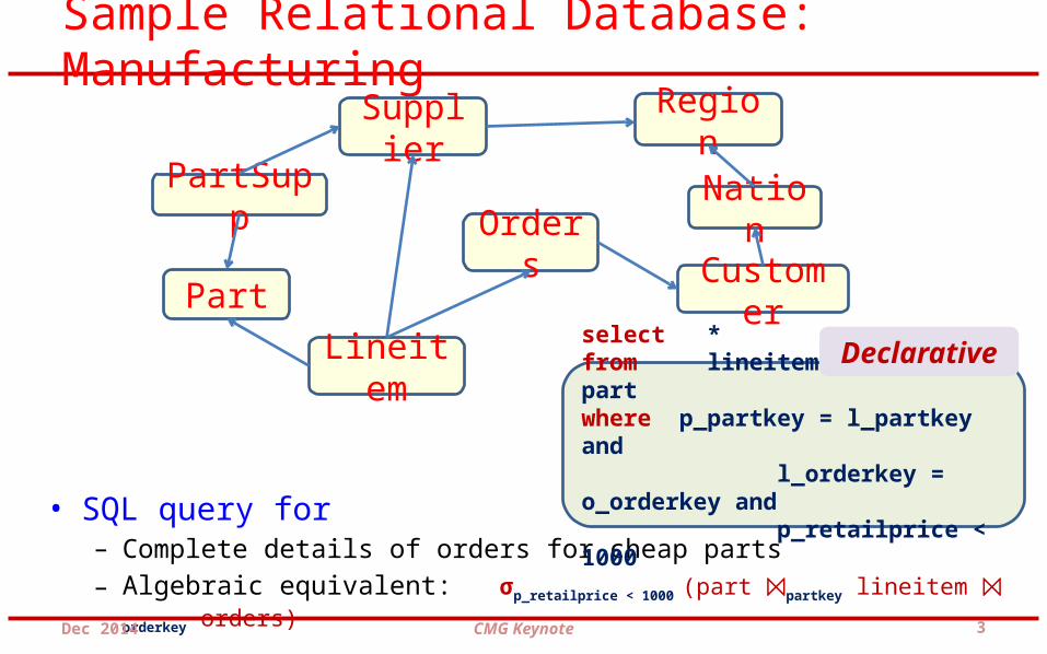
Sample Relational Database: Manufacturing

• SQL query for– Complete details of orders for cheap parts

– Algebraic equivalent: σp_retailprice < 1000 (part ⨝partkey lineitem ⨝ orderkey orders)

Dec 2014

Part

PartSupp

Supplier

Lineitem

CustomerOrders

Nation

Region

select *from lineitem, orders, partwhere p_partkey = l_partkey and l_orderkey = o_orderkey and p_retailprice < 1000

Declarative

3CMG Keynote

Query Execution Plan• Ordered (imperative) sequence of steps to process the data

• Enormous number of semantically equivalent alternative plans– for a query with N relations, there are at least N! join orders– multiple algorithmic choices at each node in the plan

(e.g. Join operator: Nested Loops, Sort Merge, Hash, Index, …)

Dec 2014

part lineitem

orders⨝ (p_partkey = l_partkey)

σ (p_retailprice < 1000)

⨝ (l_orderkey = o_orderkey)

orders lineitem

part

⨝ (p_partkey = l_partkey)

⨝ (l_orderkey = o_orderkey) σ (p_retailprice < 1000)

4CMG Keynote

Cost-based Query Optimization• Determining the most efficient plan to execute an SQL query

– Huge performance difference between good and bad plans– Only a few good plans

• Compare all alternative plans with a performance framework consisting of– operator cardinality model

• estimate the quantity of data processing at each operator• expected to accurately estimate the number of tuples at each operator

– summary statistics through histograms– operator cost model

• estimate the time taken to perform the required data processing• expected to accurately estimate the

– time taken to bring a relational page from disk to memory– time taken to process filter condition on a given tuple, etc.


Cardinality Estimation

Dec 2014

RDBMS

Statistical Metadata

2 x 104

part

6 x 106

lineitem

4 x 103

RelScan6 x 106

RelScan

1.2 x 106

Hash Join

(EQ)select *from lineitem, orders, partwhere p_partkey = l_partkey and l_orderkey = o_orderkey and p_retailprice < 1000

Query Optimizer

Estimated Selection Cardinality

Estimated Join Cardinality

Base RelationCardinality

1.2 x 106

Hash Join

1.5 x 105

orders

1.5 x 105

RelScan

6CMG Keynote

Estimated Join Cardinality

Canonical Query Optimization Framework

DeclarativeQuery (Q) Query Optimizer

Optimal [Min Cost]

Plan P(Q)

Operator Execution CostEstimation Model

function of (Hardware, DB Engine)e.g. NL Join = |Router| + |Router| x |Rinner|

Operator Result CardinalityEstimation Model

function of(Data Distributions, Data Correlations)e.g. Output Cardinality of Join = join filter factor

Dec 2014 CMG Keynote 7

Run-time Sub-optimality The supposedly optimal plan-choice from the query

optimizer may actually turn out to be highly sub-optimal when the query is executed with this plan. This adverse effect is due to errors in:(a) cost model → limited impact, < 30 %

(b) cardinality model → huge impact, orders of magnitude

• Coarse statistics, attribute value independence (AVI) assumption, multiplicative error propagation, outdated statistics, query construction, …


Proof by Authority [Guy Lohman, IBM Almaden]

Snippet from his recent Sigmod blog post on

“Is Query Optimization a “Solved” Problem?”


Selectivity Estimation Error (EQ)

Dec 2014

(EQ)select *from lineitem, orders, partwhere p_partkey = l_partkey and l_orderkey = o_orderkey and p_retailprice < 1000

part2 x 104

lineitem6 x 106

4 x 103

6 x 106

part2 x 104

lineitem6 x 1064 x 103

0

There are no orders for cheap parts

All the orders correspond to cheap parts

Run time situations

part2 x 104

lineitem6 x 1064 x 103

1.2 * 106

Optimizer assumes orders are equally likely for all prices

Compile time estimate

Hugeoverestimate

Hugeunderestimate

10CMG Keynote

Prior Research (lots!)

• Sophisticated estimation techniques– SIGMOD 1999, VLDB 2001, VLDB 2009, SIGMOD 2010, VLDB 2011, …

• Selection of Robust Plans– SIGMOD 1994, PODS 2002, SIGMOD 2005, VLDB 2008, SIGMOD 2010, …

• Runtime Re-optimization techniques– SIGMOD 1998, SIGMOD 2000, SIGMOD 2004, SIGMOD 2005, …

Several novel ideas and formulations, but lacked performance guarantees


Talk Summary

• We present “plan bouquets”, a query processing technique that completely eschews making estimates for error-prone selectivities (normalized cardinalities [0% to 100%])

• Plan Bouquet Approach: run-time discovery of selectivities using a compile-time selected bouquet of plans– provides worst case performance guarantees wrt omniscient oracle

that knows the correct selectivities • e.g. for a single error-prone selectivity, relative guarantee of 4

– empirical performance well within guaranteed bounds on industrial-strength environments


Problem Framework


Selectivity Dimensions

100%

0%

Example Query: EQselect *from lineitem, orders, partwhere p_partkey = l_partkey and l_orderkey = o_orderkey and p_price < 1000

sel (σ (part))

sel (part ⨝ lineitem)

sel (lineitem ⨝ orders)

100%

100%

SS – Selectivity Space


Performance Metrics

100%

0%sel (σ (part))

sel (part ⨝ lineitem)

sel (lineitem ⨝ orders)

100%

100%

• qe – estimated selectivity location in SS

• qa – actual run-time location in SS

• Poe – optimal plan for qe

• Poa – optimal plan for qa

qe(5%, 2%, 8%)

qa(75%, 62%, 85%)

Dec 2014 CMG Keynote

𝑺𝒖𝒃𝑶𝒑𝒕 (𝒒𝒆 ,𝒒𝒂 )=𝒄𝒐𝒔𝒕 (𝑷𝒐𝒆 ,𝒒𝒂)𝒄𝒐𝒔𝒕 (𝑷𝒐𝒂 ,𝒒𝒂)

¿

𝑴𝒂𝒙𝑺𝒖𝒃𝑶𝒑𝒕 (𝑴𝑺𝑶 )=𝑴𝑨𝑿 [𝑺𝒖𝒃𝑶𝒑𝒕 (𝒒𝒆 ,𝒒𝒂) ]∀𝒒𝒆 ,𝒒𝒂∈𝑺𝑺

𝑨𝒗𝒈𝑺𝒖𝒃𝑶𝒑𝒕 (𝑨𝑺𝑶 )=𝑨𝑽𝑮 [𝑺𝒖𝒃𝑶𝒑𝒕 (𝒒𝒆 ,𝒒𝒂) ]∀𝒒𝒆 ,𝒒𝒂∈𝑺𝑺

15

cost(P, qi) < 100

Main Assumptions• Plan Cost Monotonicity (Mandatory)• Perfect Cost Model (relaxed at end of talk)• Independent SS Dimensions (ongoing work)


q2

PCM: For any plan P and distinct selectivity locations q1 and q2

cost (P, q1) < cost (P, q2) if q1 q2

(q1 is dominated by q2 in SS)

Cost(P, q2) =100

16

Current Optimizer Behavior on One-dimensional SS


Parametric Optimal Set of Plans (POSP)( Parametric version of EQ)select *from lineitem, orders, partwhere p_partkey = l_partkey and l_orderkey = o_orderkey and SEL (PART) = $1

NL: Nested Loop Join MJ: Merge JoinHJ: Hash Join

L: LineitemO: OrdersP: Part

P1

P2P3

P4P5

Using Selectivity Injection


log-scale

log-

scal

e

18

POSP Performance Profile (across SS)

P1

P2P3

P4P5


Sub-optimality Profile (across SS)

SubOpt (1%, 99%)

= 20

SubOpt(80%, 0.01%)

= 100 MaxSubOpt = 100

AvgSubOpt = 1.8


P1

P5

P1

P5

P2P3

P4

20

Bouquet Approach in 1D SS


Bouquet Identification

P5P3

P2

P1

P1P1

P1 Bouquet = {P1, P2, P3, P5}

Step 1: Draw cost steps with cost-ratio r=2 (geometric progression).

Step 2: Find plans at intersection of optimal profile with cost steps

IC7

IC6

IC5

IC4

IC3

IC2

IC1


Bouquet Execution

P5P3

P2

P1

IC7

IC6

IC5

IC4

IC3

IC2

IC1

Let qa = 5%(1) Execute P1 with budget IC1(1.2E4)(2) Throw away results of P1 Execute P1 with budget IC2(2.4E4)(3) Throw away results of P1 Execute P1 with budget IC3(4.8E4)(4) Throw away results of P1 Execute P1 with budget IC2(9.6E4)(5) Throw away results of P1Execute P2with budget IC5(1.9E5)(6) Throw away results of P2Execute P3 with budget IC6(3.8E5) P3 completes with cost 3.4E5

qa = 5%


Stupid Idea ? Yes! Very stupid! We are expending lots and lots of wasted effort at

both planning time (producing PIC) and at execution time (throwing away work) ! Certainly a recipe for disaster …

But, with careful engineering, can actually be made to work surprisingly well → rest of talk


Bouquet Execution

P5P3

P2

P1

IC7

IC6

IC5

IC4

IC3

IC2

IC1

Let qa = 5%(1) Execute P1 with budget IC1(1.2E4)(2) Throw away results of P1 Execute P1 with budget IC2(2.4E4)(3) Throw away results of P1 Execute P1 with budget IC3(4.8E4)(4) Throw away results of P1 Execute P1 with budget IC2(9.6E4)(5) Throw away results of P1Execute P2with budget IC5(1.9E5)(6) Throw away results of P2Execute P3 with budget IC6(3.8E5) P3 completes with cost 3.4E5

Bouquet Cost = 3.4 E5 (P3) + 1.92 E5 (P2) + 0.96 E5 (P1) + 0.48 E5 (P1) + 0.24 E5 (P1) + 0.12 E5 (P1) = 7.1 E5

SubOpt (*, 5%) = 7.1/3.4 = 2.1

With obvious optimizationSubOpt(*, 5%) = 6.3/3.4 = 1.8

qa = 5%


Bouquet Performance (EQ)

MaxSubOpt = 3.1

Bouquet (Enhanced)

MaxSubOpt = 100 AvgSubOpt = 1.8

Native Optimizer

AvgSubOpt = 1.7


Bouquet (upper bound)Optimal (lower bound)

Worst Case Cost Analysis

Pk would complete within its budget

when qa ϵ (qk-1, qk]


1D Performance Bound

(Implication of PCM)

𝐂𝐛𝐨𝐮𝐪𝐮𝐞𝐭 (𝐪𝐤 −𝟏 ,𝐪𝐤 ]=𝐜𝐨𝐬𝐭 (𝐈𝐂𝟏 )+𝐜𝐨𝐬𝐭 (𝐈𝐂𝟐)+…+𝐜𝐨𝐬𝐭 (𝐈𝐂𝐤−𝟏 )+𝐜𝐨𝐬𝐭 (𝐈𝐂𝐤)¿𝒂+𝒂𝒓 +…+𝒂𝒓𝒌−𝟐+𝒂𝒓𝒌−𝟏

¿𝒂 (𝒓𝒌−𝟏)(𝒓 −𝟏)

𝐂𝐨𝐩𝐭𝐢𝐦𝐚𝐥 (𝐪𝐤−𝟏 ,𝐪𝐤 ]≥𝐚𝐫𝐤 −𝟐

Reaches minima at r = 2

MSO = 4Best performance achievable by any deterministic online algorithm!


Bouquet Architecture


Connection to Online Bidding Problem


• There is an object D with hidden value V in range (1, 100)

• Your task is to bid for D until you acquire it under the following rules:– If the bid B < V, then you forfeit B, and bid again– If the bid B ≥ V, then you pay B and acquire D

• Your goal is to minimize the worst-case ratio of your total payment to the object value, i.e. min ( (B1 + B2 + … + Bk) / V)

• Bid doubling algorithm is best possible choice

Bouquet Approach in 2D SS


2D Bouquet IdentificationCost

(normalized)

sel-Xsel-Y

CostPlansPlans Isocost ContoursIsocost Planes

Multiple Plans per contour


Characteristics of 2D Contours

sel - X

sel -Y

sel -Y

sel - X

Third quadrant coverage (due to PCM)P2

k can complete any query with actual selectivities(qa) in the shaded region within cost(ICk)

2D contours• Hyperbolic curves• Multiple plans per contour


Crossing 2D Contours

Entire set of contour plans must be executed to fully cover all locations under ICk

Covered by only one plan

in contour

sel - X

sel -Y

Covered by all plans in

contour


2D Performance Analysis• When qa ϵ (ICk-1, ICk]

𝑪𝒃𝒐𝒖𝒒𝒖𝒆𝒕 (𝐪𝐚 )=∑𝒊=𝟏

𝒌

[𝒏𝒊×𝒄𝒐𝒔𝒕 (𝑰 𝑪 𝒊 )]

Number of plans on ith contour

𝑪𝒃𝒐𝒖𝒒𝒖𝒆𝒕 (𝐪𝐚 )≤ 𝝆×∑𝒊=𝟏

𝒌

𝒄𝒐𝒔𝒕 ( 𝑰 𝑪𝒊 )

ρ = max(ni)

𝑺𝒖𝒃𝑶𝒑𝒕𝒃𝒐𝒖𝒒𝒖𝒆𝒕 (𝐪𝐚)=𝟒𝝆 (Using 1D Analysis)


Bound for N-dimensions: 𝑺𝒖𝒃𝑶𝒑𝒕𝒃𝒐𝒖𝒒𝒖𝒆𝒕 (𝐪𝐚)=𝟒× ρ𝑰𝑪𝒔𝒖𝒓𝒇𝒂𝒄𝒆

35

Dealing with large ρ • In practice, ρ can often be large, even in 100s,

making the performance guarantee of 4ρ impractically weak

• Reducing ρ– Compile Time:

• Anorexic POSP reduction [VLDB 2007]

– Run Time: • Explicit Monitoring of Selectivity Lower Bounds• Spilling-based Execution


1) Reducing ρ with Anorexic Reduction• Collapse a large set of POSP plans on a selectivity space

into a reduced cover that provides performance within a (1+ λ) factor of the optimal at all locations in the ESS.With λ = 0.2, invariably obtain a small-sized (< 10) cover.

Reduced to 5 plans


76 plans

37

MSO guarantees (compile time)

Query (dim)

ρPOSP MSO Bound (POSP) = 4ρPOSP

ρreduced

(λ=0.2)MSO Bound

(reduced)= 4ρreduced(1+λ)

Q5 (3D) 11 44 3 14.4

Q7 (3D) 13 52 3 14.4Q8 (4D) 88 352 7 33.6

Q7 (5D) 111 444 9 43.2Q15 (3D) 7 28 3 14.4

Q96 (3D) 6 24 3 14.4Q7 (4D) 29 116 4 19.2

Q19 (5D) 159 636 8 38.4

Q26 (4D) 25 100 5 24.0Q91 (4D) 94 376 9 43.2

TPC-H

TPC-DS


2) Reducing ρ with Selectivity Monitoring• When (cost-limited) execution of

plans on ICk does not complete the query, we know that qa does not lie under ICk

– but qa could lie anywhere beyond ICk

• By monitoring lower bounds onselectivities during execution (qrun)

qa can only be in first quadrant of qrun

(# of tuples at a node can only be greater

than what has already been seen)

(Pi, Pi+5 need not be executed)

lesser effective value of ρ Dec 2014 CMG Keynote

sel - X

sel -Y

39

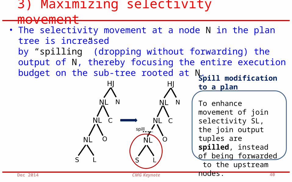
3) Maximizing selectivity movement• The selectivity movement at a node N in the plan tree is increased

by “spilling” (dropping without forwarding) the output of N, thereby focusing the entire execution budget on the sub-tree rooted at N.

Dec 2014

Spill modification to a plan

To enhance movement of join selectivity SL, the join output tuples are spilled, instead of being forwarded to the upstream nodes.

40CMG Keynote

Empirical Evaluation


Experimental Testbed

• Database Systems: PostgreSQL and COM (commercial engine)• Databases: TPC-H and TPC-DS• Physical Schema: Indexes on all attributes present in

query predicates

• Workload: 10 complex queries from TPC-H and TPC-DS – with SS having upto 5 error dimensions

• Metrics: Computed MSO and ASO using Abstract Plan Costing over SS


Performance on PostgreSQL

• For many DS queries– MSO improves from ≈106 to ≈10– ASO improves from ≈102 to ≈ 5

ASO not compromisedto reduce MSO!

BouquetNative

OptimizerLog-scale


MSO bounds

43

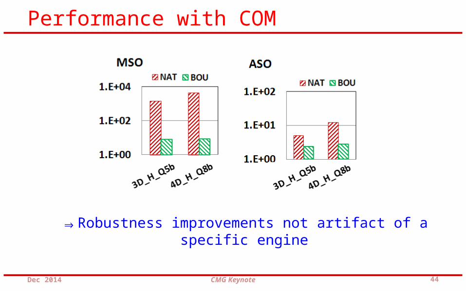
Performance with COM

⇒Robustness improvements not artifact of a specific engine


Sample Savings in Wall-clock Time

Contour ID

Avg. Execution Time (in sec)

# Executions(Enhanced Bouquet)

Time (in sec)(Enhanced Bouquet)

1 0.6 2 1.22 3.1 2 6.23 4.8 3 14.44 6.2 3 18.65 12.2 1 12.26 16.1 1 16.1

Total 12 68.7

Performance Summary

NAT(PostgreSQL)

Enhanced Bouquet

Optimal

600 sec 69 sec 16.1 sec


Query based on TPC-H Q8

In spite of uncalibrated cost model

45

Summary• Plan bouquet approach achieves

– bounded performance sub-optimality• using a (cost-limited) plan execution sequence guided by isocost

contours defined over the optimal performance curve

– robust to changes in data distribution• only qa changes – bouquet remains same

– easy to deploy• bouquet layer on top of the database engine

– repeatability in execution strategy (important for industry)• qe is always zero, depends only on qa

• independent of metadata contents

Important distinction from re-optimization

techniques


Limitations• Bouquet identification overheads are exponential in the

ESS dimensionality– unsuitable for on-the-fly queries

• Not suitable for latency sensitive applications• need to wait for final execution to complete

• Not suitable for update queries• each partial execution needs to be “garbage-cleaned” on

termination

• Not suitable for “hinted” queries• multiple plans used

• Database scaling requires bouquet re-computation• but robust to changes in data distribution


Incorporating Cost Model Error

• If cost model error is bounded by , that is

then

– for δ = 0.4 MSObounded ≤ 2 MSOperfect


For more details, visit project website:dsl.serc.iisc.ernet.in/projects/QUEST

• Concepts paper: ACM Sigmod 2014• Demo paper: VLDB 2014


Plan 1Plan 2

Plan 5

Plan 4

Plan 3Optimal Query ExecutionPerformance

Do you know the correct

selectivities ?

SQL Query

Near

Take Away


FAQs• Can we use knowledge about selectivities to reduce exploration

overheads?• lower bound and upper bound on selectivities can be utilized to limit the

selectivity space to be explored

• Overheads for high cost query instances? • Current work provides worst case relative guarantees much better than worst-

case overheads for native optimizer• we have promising results towards providing absolute guarantees (upcoming)

• Update queries• incur additional overheads as partial executions need to be “garbage-cleaned”

on termination


Plan Bouquets: A Fragrant Approach to Robust Query Processing Jayant R. Haritsa Database Systems Lab...

Documents

Transcript of Plan Bouquets: A Fragrant Approach to Robust Query Processing Jayant R. Haritsa Database Systems Lab...