P.L. Chebyshev

The Theory of Probability

Translated by Oscar Sheynin

Lectures delivered in 1879 – 1880 as taken down by A.M. Liapunov

Berlin, 2004

© Oscar Sheynin www.sheynin.de

�.�. ������� ��� ��� ������ ������, �������� � 1879 – 1880��. � ������ �.�. � ����� ������ ��������� �. . !��"��� ����� 1936 ���������

Contents

Introduction by the Translator …

Foreword by A.N. Krylov …

Chapter 1. Definite Integrals …

1.1. Preliminary Remarks and the Integrals of the First Group …

1.2. Integrals of the Second Group …

1.3. Integrals of the Third Group {Incorporating the Euler Integrals} …

1.4. Integrals of the Fourth Group {Incorporating the Fourier Integrals} …

Supplement …

Chapter 2. The Theory of Finite Differences

2.1. Direct Calculus of {Finite} Differences …

2.2. Inverse Calculus of Finite Differences …

2.3. Integration of Equations in Finite Differences …

Chapter 3. The Theory of Probability

3.1. The Laws of Probability …

3.2. On Mathematical Expectation …

3.3. On the Repetition of Events …

3.4. Application of the Theory of Probability to the Treatment of

Observations …

Index of Names …

Introduction by the Translator

1. Pafnuty Lvovich Chebyshev (Tchébichef) (1821 – 1894) was one of the two most eminent Russian

mathematicians of the 19th

century (the second, or, rather, the first one was Lobachevsky). In the theory

of probability, he proved the law of large numbers in a general form and thoroughly studied the

conditions for the central limit theorem (a term introduced by Polya in 1920) providing, in 1887, the

necessary framework for its definitive investigations carried out by his former students, Markov and

Liapunov. Chebyshev also dealt on both of these most important topics in his lectures on probability

theory that he delivered at Petersburg University from 1860 to 1882. The authoritative Russian sources

about his work are [1 – 3] and I myself published a paper [4] discussing his lectures on probability; its

conclusions would be an useful supplement to this Introduction and to my notes in the main text below1.

In 1936, Aleksei Nikolaevich Krylov, a naval architect and an applied mathematician, published

Chebyshev’s lecture notes as written down by Liapunov in 1879 – 1880 (see Krylov’s Foreword which I

am now presenting in translation below). In 1999, my translation of the lecture notes appeared as a

microfiche edition published by Verlag Dr. Hänsel-Hohenhausen in their series Deutsche

Hochschulschriften, No. 2665, Egelsbach, but the copyright to ordinary publication is mine.

2. This translation contains Chebyshev’s own footnotes as well as notes by Krylov and me (my notes

are in curly brackets), all of which are collected at the end of the appropriate subsections, and an Index of

names compiled by me.

The readers of the Russian edition undoubtedly noticed many dozens of misprints in mathematical

formulas and an almost total absence of periods after displayed formulas and (effectively) new sentences

beginning then with a lower-case first letter of their first words. The only possible explanation of this sad

state of affairs seems to be that Krylov, in spite of his testimony provided in the Foreword, had not

rewritten the original manuscript himself. The type-setter (an apprentice?) had contributed to the

wrecking of the formulas; and hardly anyone read the proofs. I have corrected the misprints without

special notice but I did not check all the formulas; and when I write something like Chebyshev had not

…, the fault can well lie elsewhere rather than with him or Liapunov.

3. I had not improved on Chebyshev’s style of oral presentation and I attempted to preserve his

mathematical terminology and notation [value of integral; exactly contrary events; mathematical

expectation (dropping however the adjective in §3.3); equations in finite differences; lim P x = 0] or used

it either more often than Chebyshev (exp [f (x)]) or throughout rather than exceptionally (i instead of #–

1). Then, I myself introduced the notation Cmn and n!. On the other hand, disregarding a single

exception, I have not retained Chebyshev’s notation (§3.3)

∏M

L

= �=

M

Lm

p(m)

for the sums of probabilities. Chebyshev transformed such sums and arrived at appropriate integrals with

limits to and t1 (say) being functions of L and M respectively. Just the same, I have not preserved his

similar use of letter S instead of � in §§3.3.9 – 3.3.10.

The numeration of the formulas was chaotic; furthermore, it did not enable the author to refer to his

previous results and he rewrote many formulas time and time again2. I ordered his numeration assigning

numbers to those formulas which were marked by asterisks or Greek or Roman letters, and the numbers

are now running consecutively through each chapter with no separate systems of them appearing

anywhere anymore. In addition, I numbered many more formulas needed for references by using a

parallel system of Roman numerals. Note that the formulas which Chebyshev included in his main

system are now printed in bold type.

In conclusion, I note that in a few cases Chebyshev had not shown

the necessary intermediate steps (§§3.1.5 and 3.3.19).

��"�� �"����� ��"�����

Notes

1. I have subsequently described Chebyshev’s work in probability [5, Chapt. 15]. In particular (pp. 205 and

206), I noted that Tikhomandritsky, in 1898, stated that in 1887 Chebyshev had remarked that it was necessary

to transform the entire theory of probability. I also described an episode proving that Chebyshev had

considered the Riemann geometry and the complex-variable analysis as trendy disciplines.

2. In this respect Markov followed his teacher.

References

1. Bernstein, S.N. (1945), Chebyshev’s work in the theory of probability. �������� ������� (Coll.

Works), vol. 4. N.p., 1964, pp. 409 – 433. Transl. in DHS 2656, 1999, pp. 67 – 96.

2. --- (1947), Chebyshev and his influence on the development of mathematics. Uchenye Zapiski Mosk. Gos.

Univ., No. 91, pp. 35 – 45. Transl. in Math. Scientist, vol. 26, 2001, pp. 63 – 73.

3. Youshkevich, A.P. (1971), Chebyshev. Dict. Scient. Biogr., vol 3, pp. 222 – 232.

4. Sheynin, O. (1994), Chebyshev’s lectures on the theory of probability. Arch. Hist. Ex. Sci., vol. 46, pp.

321 – 340.

5. --- (2004), History of the Theory of Probability to the 20th

Century. Berlin.

Chapter 1. Definite Inegrals

1.1. Preliminary Remarks and the Integrals of the First Group

1.1.0. We shall call definite only such integrals whose limits are constant magnitudes. Thus, we shall not

consider definite integrals of the type

�x

1x

dx = ln x.

Many definite integrals can be deduced from indefinite integrals but we shall only treat such of them which

cannot be determined in an indefinite form. For example, the integral

� exp (– x2) dx

cannot be determined because it represents a transcendental function unknown to us. At the same time, we can

find its value if we add the limits 0 and $; the integral will then equal #%/2. This happens because we do not

have such a function that shows how the quantity of the area OAMB 1 changes depending on the change of x.

This, however, does not preclude the possibility of determining the quantity of all the area restricted by the

curve

y = exp (– x2). (i)

In such investigations it is impossibile to apply a direct approach and we must perforce choose an indirect

way. For this reason the methods used are extremely diverse and often numerous. Definite integrals are

separated into several groups and special tricks exist for each of these. In addition, various scientists determine

one and the same integral by different methods. Our method is this: Issuing from known double integrals and

changing the order of integration, we shall determine the definite integrals. We do not aim at deriving the value

of a certain definite integral; on the contrary, we shall rather determine various definite integrals from a given

double integral.

Thus, the change in the order of integration will be the foundation of all our conclusions. Such a change is

known to be only possible if the integral might be considered as the limit of a sum; this, in turn, only holds if

the integrand remains finite within the limits of integration. For example, the integral

�−

1

1

2x

dx = = – 2

cannot therefore be regarded as the limit of a sum because the integrand is infinite at x = 0. This is even

obvious also because the integrand takes positive values for any x lying within the limits of integation so that

the equality above is impossible.

The same remark may be made concerning the integral

�−

1

1x

dx = – ln (– 1).

Its value can be represented in a somewhat different way. Since

e& i

= cos& + isin&,

it follows that

&i = ln (cos& + isin&).

Setting here & = % (2n + 1), we have

% (2n + 1) i = ln (– 1), – �−

1

1x

dx = %i (2n + 1).

This integral thus has an infinite set of different values, all of them imaginary. This can be explained by

noting that, while integrating, we could have led x through imaginary values; many paths of integration are

here possible which indeed explains the indefiniteness of the integral.

Note 1. {I do not reproduce the appended figure (which Chebyshev had not mentioned in his text). The

equation of the curve there represented was not specified and it was drawn wrongly: at point B(0; 1) the curve

(i) was not perpendicular to the axis Oy.}

1.1.1. We begin with the integral

�=

=

β

α

y

y

�∞=

=

x

x 0

e–xy

dx dy.

For the integrand to remain finite it is neceesary that ' > 0 and ( > 0. These conditions will indeed restrict

our investigation. We have

� e–xy

dx = – e–xy

/y,

therefore

�∞

0

e–xy

dx =1/y.

Then

�β

αy

dy = ln ((/ ') = �

β

α�∞

0

e–xy

dx dy = �∞

0

dx �β

α

e–xy

dy.

However,

�β

α

e–xy

dy = x

ee

x

e

x

exxxx βααβ −−−− −

=−

−−

so that

�∞

0x

eexx βα −− −

dx = ln ((/ '). (1)

This integral is almost the most important one. We shall indicate one of its applications. Supposing that ( =

n and ' = 1, we have

�∞

0x

eexx βα −− −

dx = ln n.

Assuming that n takes differenct values from 1 to (n – 1) and adding up the expressions obtained, we get

ln [(n – 1)!] = �∞

0

���

����

� +++−

− −−−−−

x

eee

x

enxnxxx )1(2 ...)1(

dx

or

ln [(n – 1)!] = �∞

0x

dx

e

eeen

x

xnxx

���

����

�

−

−−−

−

−−−

1)1( .

This integral thus allows us to express the logarithm of the product of natural numbers which is sometimes

useful.

Integral (1) is usually written down in a somewhat different form. Suppose that

x = ln (1/z), then dx = – dz/z,

�∞

0x

eexx βα −− −

dx = – �0

1z

dz

z

zz

ln−

− βα

= ln α

β

so that

�−− −

1

0

11

ln z

zzβα

dz = ln('/(). (2)

We arrived at this conclusion under the assumption that ' and ( were positive magnitudes which of course

presupposes that they were real numbers. Assuming however that they are imaginary magnitudes, and issuing

from the integral (1), we can secure some notion about the value of the integral

�∞

0x

cxsindx.

We say some notion because our assumption leads to a non-rigorous conclusion, that, like all suchlike

inferences, fails to provide, as we shall see now, the desirable results.

Suppose that ' = – ci, ( = ci where c is some real magnitude. Then

�∞

0x

eeicxicx −−

dx = ln (– 1)

and, since

[(eicx

) – (e–icx

)/2i] = sincx,

it follows that

�∞

0x

cxsin2i dx = ln (– 1) = %i

so that

�∞

0x

cxsin dx = %/2. (ii)

We have thus determined the value of this integral. However, ln (– 1) is an indefinite magnitude and %(2n

+ 1)i should have been taken instead of %i, and already this circumstance indicates that the result is doubtful

because the integral ought to have a single and quite definite value. In addition, the expression obtained does

not depend on c so that the determined value holds only for positive c’s whereas, according to the assumption

made when deriving this integral, we have only suuposed that c was a real magnitude. Strictly speaking, we

have not thus obtained the result sought.

1.1.2. Consider now the integral

�β

0

dy �∞

0

e–xy

sincx dx.

Now

� e–xy

sincx dx = – � −−

−−

y

e

y

cxexyxy sin

c cos cx dx =

– y

cxexy sin−

+ (c/y) � e–xy

cos cx dx.

Therefore

�∞

0

e–xy

sin cx dx = (c/y) �∞

0

e–xy

cos cx dx

but

� e–xy

cos cx dx = y

cxexy

−

− cos – � y

exy

−

−

(– c) sin cx dx =

(1/y) – (c/y) �∞

0

e–xy

sin cx dx.

Thus

� e–xy

sin cx dx = (c/y2) – (c

2/y

2) �

∞

0

e–xy

sin cx dx

and it follows that

�∞

0

e–xy

sin cx dx = 22 yc

c

+, �

∞

0

e–xy

cos cx dx = 22 yc

y

+. (3; 4)

These integrals are very important because they enable us to express the algebraic fractions in (3; 4) through

definiote integrals which very ofdten simplifies the solution of many problems. Note that the integrals (3; 4)

can also be determined in the indefinite form.

Supposing that y in these integrals gradually decreases tending to zero, we have, in the limit,

�∞

0

sin cx dx = 1/c, �∞

0

cos cx dx = 0.

It is easy to see, however, that the obtained integrals possess no direct sense because neither sin cx nor cos cx

approaches any definite limit as x increases to infinity. Taken by themselves, these integrals are therefore

indefinite magnitudes. Nevertheless, when considered as the limits of integrals (3; 4), they have quite a definite

value as found by us.

�∞

02

nuinuiee

−+·

22 up

du

+ =

p2

πe

– n p.

Substituting positive numbers n1, n2, … instead of n, we get in the right side factors exp (– n1 p),

exp (– n2 p), … and, multiplying the obtained integrals by A1, A2, … respectively and adding together

the results we shall find

(1/2) �∞

0

[A1exp (– n1 ui) + A2exp (– n2 ui) + … A1exp (n1 ui) +

A2exp (n2 ui) + …]22 up

du

+ =

p2

π [A1exp (– n1 ui) + A2exp (– n2 ui) + …].

Suppose now that

f (x) = A1exp (–n1 x) + A2exp (–n2 x) + … (ix)

and the last integral will become

�∞

02

)()( uifuif −+·

22 up

du

+ =

p2

πf (p). (18)

We have thus derived the required formula. The non-rigor of this derivation consists in that (18) holds only

for such functions which may be expanded into the series (ix) where A1, A2, … are some constant

coefficients, whereas, having no criteria for distinguishing between functions that may, and may

not be expanded into such a series, we consider (18) as though valid for any function.

Assuming

f (x) = A1exp (–n1 x/a) + A2exp (–n2 x/a) + …

we shall find

�∞

02

)()( auifauif −+·

22 up

du

+ =

p2

πf (ap).

Differentiating this equality with respect to a, we shall obtain

�∞

02

)()( auifauif −′−′·

22 up

ui

+du =

2

πf )(a p)

and therefore

�∞

0i

auifauif

2

)()( −′−′·

22 up

udu

+ = –

2

πf )(a p).

Denoting f )(x) = * (x) we get

�∞

0i

auiaui

2

)( )( −− ϕϕ·

22 up

udu

+ = –

2

π* (ap). (19)

If now f (x) = +) (x), the integral (18) will provide

�∞

02

)()( auiaui −′+′ ψψ

22 up

du

+ =

p2

π+)(ap).

Integrating this equality with respect to a between the limits 0 and ' we shall find

�∞

0

�α

02

)()( auiaui −′+′ ψψ

22 up

du

+ =

2

π·

2

)0() (

p

p ψαψ −.

However,

�α

0

+)(aui) da =ui

ui )0()( ψαψ −, �

α

0

+)(– aui) da =ui

ui)()0( αψψ −−

and we obtain

�∞

0ui

uiui

2

)()( αψαψ −−·

22 up

du

+ =

2

π·

2

)0() (

p

p ψαψ −

or

�∞

0i

uiui

2

)()( αψαψ −−·

)( 22 upu

du

+ =

2

π·

2

)0() (

p

p ψαψ −. (20)

Integrals (18) – (20) are to be found in a contribution by Abel and one of them is in Bertrand’s writing,

but the general formula that interests us was first given by Cauchy. We conclude here the study of the

integrals of the second group.

1.3. Integrals of the Third Group

1.3.1. The integrands of the integrals that we shall now study contain functions which could at first

sight seem to be algebraic whereas in essence they are special transcendental functions. These integrals

are of the type

�∞

0

21 x

x

+

λ

dx (x)

where , is any number. We shall therefore begin by saying a few words about algebraic functions in general.

We call algebraic only such functions that are the roots of the equation

Ao y n + A1 y

n-1 + A2 y

n-2 + … + An-1 y + An = 0

where n is an positive integral number and the coefficients Ao, A1, …, An are some integral functions of x. Functions

not fitting in with this definition no longer represent algebraic functions so that x , that cannot satisfy our equation at all

values of , is a transcendental function, but it becomes algebraic as soon as we assume that , is a commensurable

number.1

We shall now indeed consider the integral (x) at any ,. But we shall note first of all that this integral

will have a finite value only for values of , within 1 and – 1. Indeed, for , > 1 the degree of the

product x·x, = x

,+1 will be higher than 2 and the integral, in virtue of a known theorem, will be

infinite. And for , < –1, setting x = 1/z, , = – µ and µ > 1, we have

�∞

0

21 x

x

+

λ

dx = �∞

0

21 z

z

+

µ

dz.

This means that the integral will {again} be infinite. For , = ± 1 we obtain

�∞

0

21 x

x

+dx = (1/2) [ln(1 + x

2)]

0

∞ = $;

�∞

0

2

1

1 x

x

+

−

dx = �∞

0

)/1(1

)/1(2

1

z

z

+

−

[–2

z

dz] = �

∞

0

21 z

z

+dz = $.

If now , = ' + i ( it will be necessary that ' be contained between 1 and – 1. Thus, we shall

consider the integral (x) assuming that 1 > , > – 1.

Note 1. {Chebyshev’s term.}

1.3.2. We have

�∞

0

21 x

x

+

λ

dx = �1

0

21 x

x

+

λ

dx + �∞

1

21 x

x

+

λ

dx,

but

�1

0

21 x

x

+

λ

dx = �1

0

x, (1 + x

2)

– 1 dx =

�1

0

x, (1 – x

2 + x

4 – x

6 + …) dx = �

1

0

x, dx – �

1

0

x,+2

dx +

�1

0

x,+4

dx – �1

0

x,+6

dx + …

In general, however,

�1

0

x,+m

dx = [1

1

++

++

m

xm

λ

λ

]0

1 =

1

1

++ mλ

because, under our conditions regarding ,, (, + m + 1) is always positive. If , = ' + (i

then

lim (x,+m+1

) x=0 = lim (x'+m+1

x(i

) x=0.

Since ( can be negative it could seem at first sight that x(i

can be infinite, but it is not difficult to prove

that this factor cannot exceed some boundary. Indeed,

x(i

= e(i lnx

= cos (( lnx) + i sin (( lnx)

and therefore in any case

lim (x , + m + 1

)x=0 = 0

if only ' is contained within the boundaries indicated above. Thus,

�1

0

21 x

x

+

λ

dx = 1

1

+λ –

3

1

+λ +

5

1

+λ – …

The second integral is

�∞

1

21 x

x

+

λ

dx = �0

1)/1(1 2z

z

+

−λ

·[–2

z

dz] = �

1

0

21 z

z

+

−λ

dz.

But, because of the above, the last integral is equal to

1

1

+− λ –

3

1

+− λ +

5

1

+− λ – …

And so

�∞

0

21 x

x

+

λ

dx = (λ+1

1 +

λ−1

1) – (

λ+3

1 +

λ−3

1) + … =

221

12

λ−

⋅ –

223

32

λ−

⋅ +

225

52

λ−

⋅ – … (21)

We have thus expressed our integral as a series whose sum we still ought to determine.

The similarity of this expansion with the decomposition of rational fractions into partial fractions at

once arrests our attention. Indeed, we can present (21) as

�∞

0

21 x

x

+

λ

dx = 1

1

+λ –

1

1

−λ +

3

1

+λ –

3

1

−λ + …

However, any rational fraction f (x) /F (x) where F (x) has no multiple roots can be represented as

)(

)(

xF

xf =

)(

)(

1

1

xF

xf

′·

1

1

xx − +

)(

)(

2

2

xF

xf

′·

2

1

xx − +

)(

)(

3

3

xF

xf

′·

3

1

xx − + …

so that in our case the roots of F (x) are

1, 3, 5, 7, …, – 1, – 3, – 5, – 7, …

and f (x) / F (x) = 1 at any x equal to one of the roots of F (x). And we shall now determine the

function F (x) satisfying these conditions.

1.3.3. Let us consider the function

F (x) = cos(n arccos x)

where n is any integer. It is easy to show that F (x) is an integral function of the n-th degree.

Indeed, substituting arccos x = * and noting that

cos n* = [e n*i

+ e – n*i

]/2

we shall find that

F (cos *) = cos n* = [e n*i

+ e – n*i

]/2.

However, e ±n*i

= cos n* ± i sin n* so that

F (cos *) ={[cos n* + i sin n*] + [cos n* – i sin n*]}/2 =

{[cos * + i sin *]n + [cos * – i sin *]

n}/2.

Thus

F (x) = cos(n arccos x) = (1/2) [(x + 12 −x )n + (x – 12 −x )

n]. (22)

The terms that include odd degrees of the root will depend on it; however, it is not difficult to see that

they will finally cancel out so that we shall obtain for F (x) an integral rational function. Since

12 −x = x – (1/2)·(1/x) – (1/2)·(1/2)·(1/2)·(1/x3) – …

we have

x – 12 −x = (1/2)·(1/x) + (1/2)·(1/2)·(1/2)·(1/x3) + …

and the term [x – 12 −x ]n in (22) will contain only negative powers of x; all such terms will

finally cancel out with the terms containing negative powers of [x – 12 −x ]n and only the

integral part of this expression will be left. Denoting {here and in the sequel} the entire part {of a

function} by E, we can express this result as

F (x) = E {[[x – 12 −x ]n

/ 2]}.

Contributions concerning the study of such functions are mainly due to Chebyshev so that the

expression (22) is also called Chebyshev polynomial. At present, such investigations are included in

many writings on integral calculus,1 and, for example, in England they can be found in many courses in

integral calculus under the heading Chebyshev’s works. Zolotarev’s studies concern similar

issues; more precisely, issues relating not to circular but to elliptic functions. Accordingly, they are much more

complicated, but also less important than the works of Chebyshev.

Suppose now that n = 2m where m is an integer. Then

F (x) = cos (2m arcos x ) = Ao x2m

+ A1 x2m-1

+ + A2 x2m-2

+ …

We shall try to expand the function 1/F (x) into partial fractions. To attain this goal we shall find

the roots of the equation

F (x) = 0 or cos (2m arcos x ) = 0

and prove that all of them are different. It is not difficult to see that this equation is satisfied if

arccos x = m

k

4

)12( π+

where k is any integer. Assuming that it takes different values from 0 to (2m – 1), we obtain the

following roots of this equation:

k = 0, x1 = cos (%/4m); k = 1, x2 = cos (3%/4m);

k = 2, x3 = cos (5%/4m); …; k = µ, xµ+1 = cos [(2µ + 1)%/4m];

k = 2m – µ – 1, x2m – µ = cos [(4m – 2µ – 1)%/4m]; …

k = 2m – 1, x2m = cos [(4m – 1) %/4m].

Since the equation F (x) = 0 {above} is of degree 2m, it cannot have any other roots. It is seen

therefore that all of its roots are different and moreover real. For this reason our expansion will be of the

type

)(

1

xF =

)(

1

1xF ′·

1

1

xx − –

)(

1

2xF ′·

2

1

xx − + … = �

)(

1

µxF ′·

µxx −

1.

However,

F)(x) = 21

)arccos2sin(2

x

xmm

−,

F)(xµ) = 2m]4/)12sin[(

]}4/)12cos[(arccos2sin{

m

mm

πµ

πµ

−

− = 2m

]4/)12sin[(

]2/)12sin[(

mπµ

πµ

−

−.

But sin[% (2µ – 1)/2] = (– 1)µ-1

so that

F)(xµ) = (– 1)µ-1

]4/)12sin[(

2

m

m

πµ −.

Thus,

)arccos2cos(

1

xm =� 1)1( 2

]4/)12sin[(−−

−µ

πµ

m

m·

]4/)12cos[(

1

mx πµ −− =

(1/2m)� (– 1)µ-1

]4/)12cos[(

]4/)12sin[(

mx

m

πµ

πµ

−−

−

where the sums should extent consecutively over µ = 1, 2, …, 2m. We now have the following

remarkable formula

)arccos2cos(

2

xm

m =� (– 1)

µ-1

]4/)12cos[(

]4/)12sin[(

mx

m

πµ

πµ

−−

−

from which, assuming that arccos x = * and m = 1, we can derive the known formula

cos 2* = 2cos2* – 1.

For x = cos* we have

ϕm

m

2cos

2 = � (– 1)

µ-1

]4/)12cos[(cos

]4/)12sin[(

m

m

πµϕ

πµ

−−

−. (23)

We shall compare now two terms of this formula, those where µ = k and µ = (2m + 1 – k).

Introducing, in general,

- (µ) = (– 1)µ-1

]4/)12cos[(cos

]4/)12sin[(

m

m

πµϕ

πµ

−−

−

we have

- (k) = (– 1)k-1

]4/)12cos[(cos

]4/)12sin[(

mk

mk

πϕ

π

−−

−,

- (2m + 1 – k) = (– 1)2m-k

]4/)214cos[(cos

]4/)214sin[(

mkm

mkm

πϕ

π

−+−

−+ =

(– 1) k

]4/)12cos[(cos

]4/)12sin[(

mk

mk

πϕ

π

−+

−.

It is therefore seen that in our expansion the sum of the terms equally distant from the middle is

- (k) + - (2m + 1 – k) = (– 1) k-1

sinm

k

4

)12( π−·

[]4/)12cos[(cos

1

mk πϕ −− –

]4/)12cos[(cos

1

mk πϕ −+] =

(– 1) k-1

]4/)12[(coscos

]2/)12sin[(22 mk

mk

πϕ

π

−−

− =

(– 1) k-1

]sin]4/)12[(sin

]2/)12sin[(22 ϕπ

π

−−

−

mk

mk.

Formula (23) thus becomes

ϕm

m

2cos

2 = � (– 1)

k-1

]sin]4/)12[(sin

]2/)12sin[(22 ϕπ

π

−−

−

mk

mk (23�)

where k should be changed from 1 to m inclusively.

Suppose now that * tends to zero and m increases indefinitely in such a way that the product 2m *,

which we shall denote by % ,/2, remains finite. We shall try to find the limit of our sum under these

conditions. We have 2m = % ,/2*, therefore

)2/cos(

2/

λπ

ϕλπ = � (– 1)

k-1

ϕλππϕ

πλϕπ22 sin]2/2)12[(sin

]/2)12sin[(

−−

−

k

k =

� (– 1)k-1

ϕλϕ

λϕ22 sin]/)12[(sin

]/)12(2sin[

−−

−

k

k,

)2/cos(

2/

λπ

π = � (– 1)

k-1

ϕϕλλϕϕλ

λϕ22 sin)/(]/)12[(sin)/(

]/2)12sin[(

−−

−

k

k =

� (– 1)k-1

22 ]/)[(sin]}/]/)12{sin[(

]/)12(2sin[

ϕϕϕλϕλ

λϕ

−−

−

k

k.

And, since in general

lim [sin (N*)/*]*=0 = N,

[)2/cos(

2/

λπ

π]*=0 = � (– 1)

k-1

1]/)12[(

/)12(22 −−

−

λλ

λ

k

k =

� (– 1)k-1

22)12(

)12(2

λ−−

−

k

k.

Thus, we find the following expression

)2/cos(

2/

λπ

π = � (– 1)

k-1

22)12(

)12(2

λ−−

−

k

k (24)

where k should take all the integer values from 1 to $. Evidently, since , is here determined by the

condition

, = (4m*/%)*=0, m = $,

it may take all possible values including incommensurable ones.2

If , has value of the type (' +

i(), which is only possible if * takes imaginary values (because m is a real magnitude), the

obtained formula is also valid in this case, because, when determining the limit of the sum at * = 0

and m = $ by means explicated in the differential calculus (the method based on geometric

considerations that we applied in this case { ? } evidently will not do), we would have arrived at the same

expression.

Note 1. Alekseev, N.N. �� ��������� ������� (Integral Calculus).

Note 2. {Cf. Note 1 to §1.3.1.}

1.3.4. We may represent the expression (24) in such a way:

)2/cos(

2/

λπ

π =

21

12

λ−

⋅ –

23

32

λ−

⋅ +

25

52

λ−

⋅ – …

Supposing now that , is contained between the boundaries – 1 and 1, and comparing this equality with

(21), we shall have

�∞

0

21 x

x

+

λ

dx = )2/cos(

2/

λπ

π, – 1 < , < 1. (25)

We have thus found the integral sought. It is sometimes expressed in a different way. Substituting x

= ez we shall obtain

)2/cos(

2/

λπ

π = �

∞

∞−

zz

z

ee

e

+−

λ

dz = �∞−

0

zz

z

ee

e

+−

λ

dz + �∞

0

zz

z

ee

e

+−

λ

dz.

However,

�∞−

0

zz

z

ee

e

+−

λ

dz = �−∞

0

zz

z

ee

e

+

−−

− λ

dz = �∞

0

zz

z

ee

e

+−

−λ

dz

and therefore

�∞

0

zz

z

ee

ee−

−

+

+ z λλ

dz = )2/cos(

2/

λπ

π. (26)

Assuming now that , = (i, we shall get

�∞

0

zz

iziz

ee

ee−

−

+

+ ββ

dz = �∞

0

zzee

z

+−

βcos2dz =

)2/cos(

2/

iβπ

π =

2/2/ βπβπ

π−+ ee

.

Thus

�∞

0

zzee

z

+−

βcosdz =

2/2/

2/βπβπ

π

ee +−. (27)

Even more remarkable is another modification of the integral (25) to which we can arrive by

substituting x2 = z, dx = (1/2) z

–1/2 dz:

�∞

0z

z

+1

2/λ

·(1/2) z–1/2

dz = )2/cos(

2/

λπ

π,

�∞

0z

z

+

−

1

2/1 2/λ

dz = )2/cos(λπ

π.

Supposing here that ,/2 – 1/2 = n – 1, we shall find

�∞

0z

zn

+

−

1

1

dz = ])2/1cos[( π

π

−n =

)2/cos( nππ

π

− =

nπ

π

sin.

If now z = x/(1 – x) we shall have finally

�1

0

x n-1

(1 – x) –n

dx = nπ

π

sin, 0 < n < 1. (28)

In such a form this integral is a particular case of the Euler integral of the first kind

�1

0

x ,-1

(1 – x) µ-1

dx

with , = n and µ = – n – 1. We shall now go on to considering such integrals.

The Euler Integrals {§§1.3.5 – 1.3.14}

1.3.5. An Euler integral of the second kind is the integral

�∞

0

x. – 1

e – x

dx

which is usually denoted /(.) as a function of .. And, as stated above, the integral of the first kind is

�1

0

x ,-1

(1 – x) µ-1

dx.

There is no special notation for this integral; however, some authors denote it by (,; µ), others by B

(,; µ). We shall adopt the fist symbol, so that, replacing . by n, , by p and µ by q, we have

�1

0

x p-1

(1 – x) q-1

dx = (p; q), (29)

�∞

0

xn – 1

e – x

dx = /(n). (30)

In order to consider these integrals as limits of some sums it is necessary that the parameters n, p, q be

positive; otherwise, each integrand becomes infinite at one of its limits. We shall therefore assume

that n > 0, p > 0, q > 0. True, the integrand in (29) becomes infinite at each of the limits, and

in (30), at the lower limit, when the parameters being positive are less than 1. However, it can be proved

that in these cases the integrals are finite. Indeed,

�∞

0

xn – 1

e – x

dx = �1

0

xn – 1

e – x

dx + �∞

1

xn – 1

e – x

dx.

Supposing now that n is a positive proper fraction,1 we shall find that

�1

0

xn – 1

e – x

dx < �1

0

xn – 1

dx

or that

�1

0

xn – 1

e – x

dx < [xn/n]

0

1 .

This integral is thus finite at any positive n whereas

�∞

1

xn – 1

e – x

dx < �∞

1

e – x

dx < 1/e.

As to the Euler integral of the first kind, it will also be finite at the stated

values of the parameters p and q. Indeed, we shall soon prove that it is

connected wuth the integral of the second kind by the remarkable equation

(p, q) = )(/)/()(/

qp

qp

+. (31)

However, before proving this relation, we shall indicate some properties of the

Integrals of the first and the second kind beginning with the latter.

When integrating by parts, we find that

�∞

0

xn – 1

e – x

dx = [n

exxn −

]0

∞ + �

∞

0n

exxn −

dx = (1/n) �∞

0

xn

e – x

dx,

i.e., that

/(n) = (1/n) /(n + 1).

Therefore,

/(n + 1) = n /(n). (32)

In the same way

/(n + 2) = (n + 1) /(n + 1), /(n + 3) = (n + 2) /(n + 2), …

/(n + m) = (n + m – 1) /(n + m – 1).

Multiplying these equalities we obtain

/(n + m) = n (n + 1) (n + 2) … (n + m – 1) /(n).

Assuming that n = 1 and noting that

/(1) = �∞

0

e – x

dx = 1

we find for any integral m the following equality

/(m + 1) = m!. (33)

It is seen now that /(2) = 1 = /(1) so that between 1 and 2 the function / ought to have a minimum (the

second derivative of /(n) is always positive). Consider now the integral

(p; q) = �1

0

x p–1

(1 – x) q–1

dx

where p is supposed to be any positive number and q, a positive integer greater than 1. Integrating by parts,

we find that

(p; q) = [(x p/p) (1 – x)

q–1]0

1 + (1/p) �

1

0

x p

(q – 1) (1 – x) q–2

dx

so that

(p; q) = [(q – 1)/p] (p + 1; q – 1).

Hence

(p + 1; q – 1) = [(q – 2) / (p + 1)] (p + 2; q – 2),

(p + 2; q – 2) = [(q – 3) / (p + 2)] (p + 3; q – 3),

(p + k; q – k) = [(q – k – 1) / (p + k)] (p + k + 1; q – k – 1)

if only we admit the inequality q – k > 1.

Multiplying these equalities we obtain

(p; q) = ))...(1(

)1)...(2)(1(

qppp

kqqq

++

−−−− (p + k + 1; q – k – 1).

Assuming that q – k = 2 we get

(p; q) = )2)...(1(

)!1(

−++

−

qppp

q (p – q – 1; 1).

This equality will be valid for any positive p and positive integer q. However,

(p + q – 1; 1) = �1

0

x p+q–2

dx = 1

1

−+ qp.

Therefore, we obtain, for such values of p and q,

(p; q) = )1)...(2)(1(

)!1(

−+++

−

qpppp

q. (34)

If we assume now that p is also an integer, then it follows that

(p; q) = )!1(

)!1()!1(

−+

−−

qp

pq =

)(/)(/)(/

qp

pq

+.

And so, the equation (31) is proved for integer values of p and q.

Note 1. {Here, and in many cases in the sequel, Chebyshev as though avoids irrational numbers.}

1.3.6. In order to prove the validity of (31) in the general case, we consider the double integral

I = �∞

0

�∞

0

x p–1

e – x y

y p+q–1

e – y

dx dy.

Integrating first with respect to x, and then to y, and substituting xy = z, we shall have

�∞

0

x p–1

e –x y

dx = (1/y p) �

∞

0

z p–1

e – z

dz = = py

p)(/,

I = �∞

0

p

qp

y

y1−+

/(p) e – y

dy = /(p) /(q).

Integrating now in the other order and assuming that y (x + 1) = u, we find that

�∞

0

y p+q–1

e – y (x + 1)

dy = qpx ++ )1(

1 �

∞

0

u p+q–1

e – u

du =

qpx ++ )1(

1/(p + q),

�∞

0

qp

p

x

x+

−

+ )1(

1

/(p + q) dx = /(p + q) �∞

0

qp

p

x

x+

−

+ )1(

1

dx.

Therefore

�∞

0

qp

p

x

x+

−

+ )1(

1

dx =)(/

/(q))(/qp

p

+. (xi)

Supposing that p + q = 1 and using formula (28) we may incidentally derive the following

remarkable formula

/(p) /(1 – p) = π

π

psin (35)

which is very important in the practical sense for compiling tables of the values of the function /. It

shows that, within the interval (0; 1), it is sufficient to calculate the values of / only for the argument not

exceeding 1/2; the other values will be determined by formula (35).

We return now to the integral (xi). Assuming that x = z / (1 – z) so that 1/(1 + x) = 1 – z and dx

= dz/(1 – z)2, we obtain

�1

0

qp

p

x

x+

−

+ )1(

1

dx = �1

0

1

1

)1( −

−

− p

p

z

z(1 – z)

p+q

2)1( z

dz

− =

�1

0

z p–1

(1 – z) q–1

dz = (p; q),

hence (31). This equation shows that (p; q) is a symmetric function of p and q which can also be

proved directly by setting z = 1 – y:

(p; q) = �1

0

z p–1

(1 – z) q–1

dz = – �0

1

(1 – y) p–1

y q–1

dy =

�1

0

y q–1

(1 – y) p–1

dy = (q; p).

Thus, the validity of the equation (31) is proved for all values of p and q for which the double

integral at the very beginning of this subsection might be considered as the limit of a sum. This last is true for

any positive p and q because, when integrating in the first order, we arrive at the product /(p) /(q),

and, according to the above, each of these two factors is finite for all positive values of p and q.

1.3.7. Assuming that p = 1/2 in (35), we have

/(1/2) = #%. (xii)

But, in accord with (9),

�∞

0

exp (– x2) dx = (1/2) /(1/2).

The same result can also be obtained directly by setting x2 = z. Then, indeed,

�∞

0

exp (– x2) dx = �

∞

0

e – z

(1/2) z – ½

dz = (1/2) �∞

0

z1/2 – 1

e – z

dz =

(1/2) /(1/2).

1.3.8. A remarkable equation connecting the values of the / function can be derived from equation (31).

Supposing that p = q we have here

(p; p) = )2(/

/(p))(/p

p.

Transforming the left side of this equality we obtain

(p; p) = �1

0

x p–1

(1 – x) p–1

dx = �1

0

[x (1 – x)] p–1

dx =

�1

0

{(1/4) – [x – (1/2)]2}

p–1dx = (1/4)

p–1 �

1

0

[1 – (2x – 1)2]

p–1dx.

Setting 2x – 1 = z we arrive here at

(p; p) = 14

1−p �

−

1

1

(1 – z2)

p – 1 (1/2) dz =

14

1−p �

1

0

(1 – z2)

p – 1 dz

because the integrand is an even function. Assuming now that z2 = u, we find that

(p; p) = 14

1−p �

1

0

(1 – u) p – 1

(1/2) u – ½

du =

122

1−p �

1

0

u ½ – 1

(1 – u) p –1

du = 122

1−p

(1/2; p).

Thus,

)2(/

/(p))(/p

p =

122

1−p 1/2) /(

)/()2/1(/+p

p

and, on the strength of (xii), we obtain

/(p) /(p + 1/2) = 122 −p

π /(2p). (36)

This remarkable formula was first discovered by Legendre.

1.3.9. Let us now go over to integrals expressed by the logarithm of gamma. In §1.1.1 we found that for any

positive and integer n

ln [(n – 1)!] = �∞

0x

e

eeen

x

xnxx

−

−−−

−

−−−

1 )1(

dx

and on the strength of formula (33) this is equal to ln /(n).

We shall prove that this formula is valid for any values of n for which /(n) can be taken. We have, in

general, formula (30). Differentiating it with respect to n, we obtain

d /(n) / d n = �∞

0

e – x

x n – 1

ln x dx.

But, in virtue of formula (1), we have

ln x = �∞

0z

eezxz −− −

dz.

Therefore

d /(n) / d n = �∞

0

e – x

x n – 1

�∞

0z

eezxz −− −

dz dx =

�∞

0

�∞

0

e – x

x n – 1

z

eezxz −− −

dz dx.

Integrating here with respect to x, we arrive at

�∞

0

e – x

x n – 1

(e – z

– e – x z

) dx = e

– z

�∞

0

xn – 1

e – x

dx – �∞

0

e – x (1 + z)

x n – 1

dx

and, setting x (1 + z) = t, we obtain

�∞

0

e – x (1 + z)

x n – 1

dx = nz)1(

1

+ �

∞

0

e – t

t n – 2

dt = nz

n

)1(

)(/+

so that

d /(n) / dn = �∞

0

[e – z

– (1 + z) – n

] /(n) z

dz,

hence

dn

nd )(/ )(/

1

n =

dn

nd )(/ln = �

∞

0

[e – z

– (1 + z) – n

] z

dz.

It follows that

�n

1

d ln/(n) = ln /(n) = �∞

0

�n

1

[e – z

– (1 + z) – n

] z

dz dn,

ln /(n) = �∞

0

(n – 1) e – z

z

dz – �

∞

0

[)1ln(

)1(

z

zn

+−

+ −

]1

n

z

dz.

Thus

ln /(n) = �∞

0

[(n – 1) e – z

+ )1ln(

)1()1( 1

z

zzn

+

+−+ −−

] z

dz.

Noting now that /(2) = 1, we have

0 = �∞

0

[e – z

+)1ln(

)1()1( 12

z

zz

+

+−+ −−

] z

dz

and, consequently,

�∞

0

[(n – 1) e – z

+ (n – 1) )1ln(

)1()1( 12

z

zz

+

+−+ −−

]z

dz = 0.

Subtracting this equality from the preceding one we shall have

ln /(n) = �∞

0)1( ln

])1()1)[(1()1()1( 211

z

zznzzn

+

+−+−++−+ −−−−

z

dz

and, assuming that ln (1 + z) = x, we find that

ln /(n) = �∞

0

[e – nx

– e – x

+ (n – 1)e – x

(1 – e – x

)]1−x

x

e

e

x

dx.

Finally, it follows that

�∞

0

[(n – 1) e – x

– x

nxx

e

ee−

−−

−

−

1]

x

dx = ln /(n). (37)

1.3.10. Replacing n by (n + 1) in (37) we have

ln /(n + 1) = �∞

0

[ne – x

– x

xnx

e

ee−

+−−

−

−

1

)1(

] x

dx. (38)

This formula is extremely important in mathematics and, especially, in the theory of probability where it

is applied for integer and very large values of n. We shall dwell on it also because remarkable corollaries

follow from it.

If n is a very large number, it will be more convenient to represent this formula in such a way that its

right side consists of two parts, one of them including all the finite and very large terms and the other one

serving as a supplement and including only very small terms and vanishing at n = $. This is

necessary for example when calculating ln /(n + 1) for very large values of n. We shall indeed

derive this logarithm. The integrand in (38) can be represented as

[ne – x

– x

xnx

e

ee−

+−−

−

−

1

)1(

] x

1 = [ne

– x –

x

x

e

e−

−

−1 +

x

x

e

e−

−

−1e

– nx]

x

1.

But

x

x

e

e−

−

−1 =

... !3/ !2/

... !3/ !2/132

32

−+−

+−+−

xxx

xxx =

x

1 –

2

1 + * (x)

where * (x) is the sum of all the other terms of the expansion. It is not difficult to see that * (x) includes

only positive powers of x because its term containing x in the lowest degree is x/12, so that * (x) / x

will have a finite limit at x = 0. We thus have

[ne – x

– x

xnx

e

ee−

+−−

−

−

1

)1(

] x

1 = [ne

– x –

x

x

e

e−

−

−1 + (

x

1 –

2

1) e

– nx]

x

1 +

x

x)( ϕ e

– nx.

However,

* (x) = x

x

e

e−

−

−1 +

2

1

x

1

)1(2

12x

xx

e

ee−

−−

−

−+ –

x

1 =

2

1[

x

x

e

e−

−

−

+

1

1 –

x

2]

and therefore

ln /(n + 1) = �∞

0

[ne – x

– x

x

e

e−

−

−1 + (

x

1 –

2

1) e

– nx]

x

dx +

(1/2) �∞

0

[x

x

e

e−

−

−

+

1

1 –

x

2] e

– nx

x

dx.

Or, supposing that the two integrals are denoted by F(n) and 0(n) respectively, we obtain

ln /(n + 1) = F(n) + 0(n).

We thus reduced our expression to the desired form: the function 0(n) is represented by an integral of a

function taking finite and very small values at all values of x contained within and including the

limits of integration, – and, moreover, taking very small values at very large values of n. This function has

exactly those properties which, according to our assumption, should be possessed by the second part of

the expression sought.

It is only left to determine the type of the functions F(n) and 0(n). To find the first of them we

differentiate this {yet unknown} function with respect to n:

F ) (n) = �∞

0

[e – x

– x (x

1 –

2

1) e

– nx]

x

dx =

�∞

0

[e – x

– e – nx

+ (x/2) e – nx

] x

dx.

It follows that

F ) (n) = �∞

0x

eenxx −− −

dx + (1/2) �∞

0

e – nx

dx = ln n + (1/2)·(1/n)

and

F(n) = � ln n dn + (1/2) � n

dn = n ln n – n + (1/2)ln n + C (xiii)

where C is a constant that for the time being we leave indefinite. Thus,

F(n) = C + n ln n – n + (1/2) ln n.

It ought to be noted here that the differentiation applied by us destroyed the constant C in whose

determination all the difficulty really consists. We were able to calculate the function F(n) in such an

indefinite form without any trouble exactly because of this differentiation.

Let us now investigate the function 0(n). Here, we cannot carry the integration to its conclusion and

have to express 0(n) by a series. We have

x

x

e

e−

−

−

+

1

1 =

2/2/

2/2/

xx

xx

ee

ee−

−

−

+

so that the integrand becomes

(1/2) [2/2/

2/2/

xx

xx

ee

ee−

−

−

+ –

x

2 ]

x

1e

– nx.

The product of the first two factors is here an even function {see below} so that it is possible to say at

once that its expansion into powers of x will be of the form

A1 + A2 x2 + A3 x

4 + …

We have

e ± x/2

= 1 ± x/2 + (1/2!) (x/2)2 ± (1/3!) (x/2)

3 + …,

e x/2

+ e – x/2

= 2[1 + (1/2!) (x/2)2 + …]

e x/2

– e – x/2

= 2[(x/2) + (1/3!) (x/2)3 + …]

and

2/2/

2/2/

xx

xx

ee

ee−

−

−

+ =

...48/2/

...8/12

2

++

++

xx

x =

x

2 +

6

x + …

Therefore

(1/2) [x

x

e

e−

−

−

+

1

1 –

x

2] = (1/2) [

x

2 +

6

x + … –

x

2] =

12

x + …

Thus, A1 = 1/12. Taking into account a larger number of terms in the numerator and the denominator

and carrying out the division, we shall obtain, in the same way, A2, A3, …The numbers that express

these coefficients are very closely related to the Bernoulli numbers; at present, very many

mathematicians are studying them.

So, we have

0(n) = �∞

0

[A1 x + A2 x3 + A3 x

5 + …] e

– nx

x

dx =

A1 �∞

0

e – nx

dx + A2 �∞

0

x2 e

– nx dx + A3 �

∞

0

x4 e

– nx dx + …

Noting that, in general,

�∞

0

x l–1

e – nx

dx = �∞

0

1

1

−

−

l

l

n

ze

– nx dx/n = (1/n

l ) �

∞

0

z l–1

e – z

dz = l

n

l)(/

and that, for any integer and positive values of l, /(l) = (l – 1)!, we obtain

0(n) = (1!/n) A1 + (2!/n3) A2 + (4!/n

5) A3 + … (39)

We have thus expressed 0(n) by a series depending on the coefficients A1, A2, A3, … Therefore, to say

something general about this equality, it is necessary to know the law of their composition. However, the

method of their determination applied above does not provide this law and we shall derive{other} expressions

for these coefficients, awkward for calculation but very convenient for our present purpose.

1.3.11. Setting x/2 = &i we obtain

x

x

e

e−

−

−

+

1

1 =

2/2/

2/2/

xx

xx

ee

ee−

−

−

+ =

ii

ii

ee

ee

θθ

θθ

−

−

−

+ =

θ

θ

sin2

cos2

i =

i

θctg .

But, in general,

sin & = & [1 – (&2/%2

)] {1 – [&2/(2%)

2]} {1 – [&2

/(3%)2

]} …

so that

ln sin & = ln & + ln [1 – (&2/%2

)] + ln {1 – [&2/(2%)

2]} +

ln{1 – [&2/(3%)

2 ]} + …

Differentiating this equality we have

ctg & = θ

1 –

22

2

θπ

θ

− –

22)(2

2

θπ

θ

− –

22)(3

2

θπ

θ

− – …,

(1/2) [ctg& – (1/&)] = 22 θπ

θ

− –

22)2( θπ

θ

− –

22)(3 θπ

θ

− – …

However, since in general

[1/(1 – ')] = 1 + ' + '2 + '3

+ … + 'l +

α

α

−

+

1

1l

and

22)(

1

θπ −m =

2)(

1

mπ 2)/(1

1

mπθ−,

it follows that

22

2

) (

) (

θπ

π

−m

m = 1 +

2

2

)( mπ

θ +

4

4

)( mπ

θ + … +

l

l

m 2

2

)(π

θ +

2 2

2 2

)( +

+

l

l

mπ

θ22

2

)(

)(

θπ

π

−m

m.

Therefore

22)( θπ

θ

−m =

2)( mπ

θ +

4

3

)( mπ

θ +

6

5

)( mπ

θ + … +

2 2

1 2

)( +

+

l

l

mπ

θ +

4 2

3 2

)( +

+

l

l

mπ

θ22)(

1

θπ −m.

Assuming that m takes here different values beginning with 1 and adding the thus obtained equalities

we shall have

22 θπ

θ

− +

22)(2 θπ

θ

− +

22)(3 θπ

θ

− + … = (&/%2

) [1 + (1/22) +

(1/32) + …] + (&3

/%4) [1 + (1/2

4) + (1/3

4) + …] + … +

(&2l+1/%2l+2

) [1 + (1/22l+2

) + (1/32l+2

) + …]

4 2

3 2

+

+

l

l

π

θ{

22

1

θπ − +

])2[(2

1224 2 θπ −+l

+ ])3[(3

1224 2 θπ −+l

+ …} =

(1/2) [ctg & – (1/&)].

But & = x/2i = – i x/2 so that

(1/2) [2/2/

2/2/

xx

xx

ee

ee−

−

−

+ –

x

2] i = – (S2/%

2) (–x i/2) – (S4/%

4) (–x i/2)

3 –

(S6/%6) (–x i/2)

5 – …–

2 2

1+lπ

{4/

122

x+π +

]4/)2[(2

1222 xl ++ π

+ …}·

[(–x i/2)2l+3

]

where the notation introduced is obvious. Hence

(1/2) [2/2/

2/2/

xx

xx

ee

ee−

−

−

+ –

x

2] = (S2/2%

2) x – (S4/2

3%4)x

3 +

(S6/25%6

) x5 – … + (– 1)

l

2 212

22

2 +++

ll

lS

π x

2l+1 +

(– 1) l+1

2 23 22

1++ ll π

[4/

122

x+π +

]4/2[2

1222 2 xl ++ π

+ …] x 2l+3

.

It is seen now that

A1 = (1/2%2) S2 = (1/2%2

) [1 + (1/22) + (1/3

2) + …],

A2 = – (1/23%4

) S4 = (1/23%4

) [1 + (1/24) + (1/3

4) + …],

A3 = (1/25%6

) S6 = (1/25%6

) [1 + (1/26) + (1/3

6) + …],

and in general, that

Al+1 = 2 21 22

)1(++

−ll

l

πS2l+2 =

2 21 22

)1(++

−ll

l

π[1 +

2 22

1+l

+ 2 23

1+l

+ …].

We thus have

0(n) = �∞

0

{A1 x + A2 x3 + A3 x

5 + Al+1 x

2l+1 –

2 23 22

)1(++

−ll

l

π·

[4/

122

x+π +

]4/)2[(2

1222 2 xl ++ π

+ …] x2 l+3

}e – nx

(dx/x)

and, taking into account the equality (39),

0(n) = (A1/n) + A2 [/(3) / n3] A3 [/(5) / n

5]+ … + A l+1

1 2

)1/(2+

+l

n

l –

2 23 22

)1(++

−ll

l

π�∞

0

[4/

122

x+π + …] e

– nx x

2l+2 dx.

And so, we have expressed 0(n) by a series whose terms are alternatively positive and negative and the

sign of whose additional term {remainder} is opposite to that of its preceding term. Such series are called

limitative. They possess a remarkable property: their additional term is always numerically less than the

term subsequent to the last one considered. Indeed, let us take the series

X = u1 – u2 + u3 – … ± un � Rn),

X = u1 – R1; or, u1 – u2 + R2; or, u1 – u2 + u3 – R3, etc.

It is seen that

R1 < u2; R2 < u3; …; Rn < un+1.

Therefore, such series always enable us to determine the error taking place when calculating their

{approximate} sum and this is their advantage over other series. However, they also suffer from a serious

shortcoming: they provide no clue for determining when should we stop in order to obtain the most precise

value of the sum. Indeed, in such series each term can be {numerically} either greater or less than its

preceding term. When breaking off at some term ± uk, we will note that in one case the addition of one more

term, � uk+1), can lower, and in another case it can heighten the degree of approximation. In general, as it is

seen from what was said about these series, we should stop at such a term ul whose subsequent neighbor –

ul+1 is least; the sum, calculated in such a way, will be the most precise and differ from the real sum less than

by ul+1.

Formula (39) shows that at first the terms of the series expressing 0(n) will decrease, but that, beginning

with some term, they will increase. Therefore, in order to determine, in this case, the term at which we should

break off, we ought to have ul > ul–1 or ul / ul+1 > 1 and to determine the least value of l satisfying this

inequality. We shall show how to acquire some notion about the least boundary of l by means of this

inequality.

We have

ul = Al /(2l – 1) /n 2l–1

, ul–1 = Al–1 /(2l – 3) /n 2l–3

,

1−l

l

u

u =

1 2

1

3 2

)32(/

)1/(2−

−

−

−

−l

l

l

l

nlA

nlA = (Al /Al–1) (2l – 2) (2l – 3) (1/n

2)

where only the numerical values of Al and Al–1 are taken into account. We shall thus have a conjectural

inequality

(Al /Al-1 ) (2l – 2) (2l – 3) > n2

or

(1/22%2

) ...)3/1()2/1(1

...)3/1()2/1(12222

22

+++

+++−− ll

ll

(2l – 2) (2l – 3) > n2. (40)

Now we may conclude that inequality

(2l – 2) (2l – 3) > 22%2

n2

also exists so that (2l)2 > (2%n)

2 and

2l > 2%n, l > %n. (41)

Thus we see that l should not be less than %n. However, the method of obtaining this lower boundary

does not provide the possibility of seeing whether, for l > %n, ul will really be the least, having the

least value satisfying this inequality. We went over from inequality (40) to (41), but, evidently,

we had no right to go in the other direction. It is therefore seen that %n provides only an approximate

notion about how great should l be.

We have remarked (§1.3.10) that the coefficients A1, A2, … are very closely related to the

Bernoulli numbers B1, B2, … The dependence between them is expressed by the equation

Al = (– 1) l–1

)!(2

l

B l

so that

A1 = B1/2!, A2 = – B2/4!, A3 = B3/6!, etc.

The Bernoulli numbers play a rather important part in mathematics, and, accordingly, very many treatises

are expressly devoted to studying their properties.

1.3.12. Let us now go over to the determination of the constant C in the expression (xiii). Taking the

logarithms of both sides of the Legendre formula (36)

/(n) /[n + (1/2)] = (#% / 22n–1

) /(2n)

we have

ln /(n) + ln / [n + (1/2)] = ln #% + ln / (2n) – (2n – 1) ln 2.

However,

ln /(n + 1) = C + n ln n – n + (1/2) ln n + 0 (n)

and therefore

ln /(n) = C + (n – 1) ln (n – 1 ) – n + 1 + (1/2) ln (n – 1) + 0(n – 1),

ln /[n + (1/2)] = C + [n – (1/2)] ln [(n – (1/2)] – n + (1/2) +

(1/2) ln [n – (1/2)] + 0 [n – (1/2)],

ln /(2n) = C + (2n – 1) ln (2n – 1) – 2n + 1 + (1/2) ln (2n – 1) + 0 (2n – 1).

We thus obtain such an equation:

2C + [n – (1/2)] ln (n – 1) + n ln [n – (1/2)] – 2n + (3/2) + 0 (n – 1) +

0 (n – 1/2) = ln #% + C + [2n – (1/2)] ln (2n – 1) + 1 – 2n +

0 (2n – 1) – (2n – 1) ln 2

so that

C = ln #% + [2n – (1/2)] ln (2n – 1) – [n – (1/2)] ln (n – 1) –

n ln [n – (1/2)] – (1/2) – (2n – 1) ln 2 – 0 (n – 1)

0 [n – (1/2)] + 0 (2n – 1).

However, in general we have

ln (x – 1) = ln {x [1 – (1/x)]} = ln x + ln [1 – (1/x)] = ln x –

(1/x) – (1/2) (1/x2) – …

and therefore

ln (2n – 1) = ln 2n – (1/2n) – (1/8n2) – …

ln (n – 1) = ln n – (1/n) – (1/2n2) – …,

ln [n – (1/2)] = ln (2n – 1) – ln 2 = ln n – (1/2n) – (1/8n2) – …

And so

C = ln#% + [2n – (1/2)] [ln n + ln 2 – (1/2n) – (1/8n2)] – [n – (1/2)]·

[ln n – (1/n) – (1/2n2) – …] – n [ln n – (1/2n) – (1/8n

2)] – (1/2) –

(2n – 1) ln 2 + 0(2n – 1) – 0(n – 1) – 0[n – (1/2)]

or

C = ln #% + (1/2) ln 2 – {[2n – (1/2)] /2n} + {[n – (1/2)]/n} –

{[(2n – (1/2)]/8n2} + {[n – (1/2)/]2n

2} + (1/8n) + … + 0(2n – 1) –

0(n – 1) – 0[n – (1/2)].

Assuming now that in this equation or identity (it should hold for all values of n) n = $, and noting

that 0 ($) = 0, we find that

C = ln#% + (1/2) ln 2 = ln#2%.

Thus

ln /(n + 1) = ln#2% + n ln n + (1/2) ln n – n + 0(n) (xiv)

so that

/(n + 1) = π2 n n+1/2

e –n+0(n)

.

But ·

e 0(n)

= e(1/12n) +…

= 1 + (1/12n) + …

and we thus finally obtain

/(n + 1) = π2 n n+1/2

e –n

[1 + (1/12n) + …]. (42)

If n is an integer we shall get

n! = π2 n n+1/2

e –n

[1 + (1/12n) + …].

This formula that enables us to calculate the approximate value of the product of natural numbers is due

to Stirling.1

Note 1. {In 1730, De Moivre derived this formula independently from and simultaneously with Stirling; the

latter only communicated to him the value of the constant. De Moivre also published a table of lg n! for

n = 10 (10 ) 900 with 14 decimals of which 11 or 12 were correct.}

1.3.13. In concluding the section on the Euler integrals we shall derive the famous Gauss equation

connecting {various values of} gamma. We may always suppose that

/(n) /[n + (1/m)] /[n + (2/m)] …/[n + (m – 1)/m] = F (n; m) /(nm).

Let us now try to determine the function F (n; m). We have

/(a) /[a + (1/m)] /[a + (2/m)] … /[a + (m – 1)/m] / /(am) = F (a; m).

Substituting here (a + 1) instead of a and recalling equality (32) we shall find that

)(/

)//()/(1

0

mam

miamiam

i

+

++∏−

= = F (a + 1; m)

or

)(/)...2( )1(

]/)1()...[/2)(/1(

ammammamma

mmamamaa

−+−+

−+++·

/(a) /[a + (1/m)] … /{[a + (m – 1)/m]} = F (a + 1; m),

mammammam

mmamamamam )...2( )1(

)1)...(2( )1(

−+−+

−+++ F (a; m) = F (a + 1; m),

);(

);1(

maF

maF + = m

–m =

am

ma

m

m

)1(

−

+−

and consequently

ma

m

maF)1(

);1(+−

+ =

mam

maF

);(−

.

Thus, assuming that in general m km

F (k; m) = & (k), we have

& (a) = & (a + 1) so that & (a) = & ($). Therefore

)(/

]/)1([/).../2(/)/1(/)(/am

mmamamaa −+++ = m

–a m lim [& (x)] x =$

where

& (x) = xmmmx

mmxmxmxx )(/

]/)1([/).../2(/)/1/()(/−

−+++.

Therefore

ln & (x) = ln /(x) + ln / [x + (1/m)] + … + ln /{x + [(m – 1)/m]} +

m x ln m – ln /(m x).

But because of (xiv)

ln & (x) = ln π2 + [x – (1/2)] ln (x – 1) – x + 1 + 0 (x – 1) +

ln π2 + [x – (1/2) + (1/m)] ln[x – 1 + (1/m)] – x + 1 – (1/m) +

0 [x – 1 + (1/m)] + ln π2 + [x – (1/2) + (2/m)] ln[x – 1 + (2/m)]

– x – 1 – (2/m) + 0 [x – 1 + (2/m)] + … + ln π2 +

{x – (1/2) + [(m – 1)/m]} ln{x – 1 + [(m – 1)/m]} – x + 1 –

[(m – 1)/m] + 0 {x – 1 + [(m – 1)/m)]} – ln π2 –

[mx – (1/2)] ln (mx – 1) + mx – 1 + mx ln m – 0 (mx – 1).

Noting that in general

ln (x – r) = ln [x (1 – (r/x)] = ln x + ln[1 – (r/x)] = ln x – r/x – …

we find that

ln & (x) = (m – 1) ln π2 + [x – (1/2)] [ln x – (1/x) + …] +

0 (x – 1) + [x – (1/2) + (1/m)] {ln x – [1 – (1/m)]/x} +

0 [x – 1 + (1/m)] + [x – (1/2) + (2/m)] {ln x – [1 – (2/m)]/x} +

0 [x – 1 + (2/m)] + … + {x – (1/2) + [(m – 1)/m]}·

[ln x – x

mm /)1(1 −−] + 0 {x – 1 + [(m – 1)/m]} + m x ln m +

(m – 1) – {[(1 + 2 + … + (m – 1)]/m} –

[m x – (1/2)] [ln mx – (1/mx) – …] – 0 (mx – 1)

and

ln & (x) = (m – 1) ln π2 + mx ln x + mx ln m – mx ln mx + m –

1 + 1 + (1/2) ln mx – [1 + 2 + … + (m – 1)]/m – (1/2) m ln x –

m + [1 + 2 + … + (m – 1)]/m + m

m )1(...21 −+++ln x + … +

0 (x – 1) + 0 [x – 1 + (1/m)] + … + 0 {x – 1 + [(m – 1)/m]} –

0 (mx – 1).

Therefore

ln & (x) = (m – 1) ln π2 + (1/2) ln m + …

We have retained only two terms because all the rest of them vanish at x = $. And so

lim [ & (x)] x =$ = (m – 1) ln π2 + ln #m

which means that

lim [ln & (x)] x =$ = #m (2%) (m–1)/2

; F(a; m) = m – am+1/2

(2%) (m–1)/2

and

)(/

]/)1([/).../2(/)/1(/)(/am

mmamamaa −+++ = m

–a m+1/2 (2%)

(m–1)/2.

Thus we have

/(,) /[, + (1/m)] … /{, + [(m – 1)/m]} = m –, m–1/2

(2%) (m–1)/2 /(m,). (43)

This equation which is valid for any , and any integral and positive m is a generalization of equation (36).

Assuming here that , = 1 and supposing that n is an integral positive number, we obtain

/[1 + (1/n)] /[1 + (2/n)] … /{1 + [(n – 1)/n]} = n– n+1/2 (2%)

(n–1)/2 /(n).

It follows that

1

)!1(−

−n

n

n/(1/n) /(2/n) ... /[(n – 1)/n] = n– n+1/2

(2%)(n–1)/2

/(n)

and in virtue of the equality (33)

/(1/n) /(2/n) ... /[(n – 1)/n] = (2%)(n–1)/2

n–1/2. (44)

1.3.14. We defined /(,) as the value of the definite integral {see (30)}

�∞

0

x ,–1

e – x

dx.

Accordingly, we have necessarily considered the gamma function only for such values of , for which this integral

had sense, i.e., for which it was the limit of some sum. We saw that these values were contained within 0 and $.

There exists, however, another more general definition of the gamma {function}. The values of this function are

extended onto such cases where the variable also takes negative values. Exactly this last fact gave the occasion for

the new definition and in order to go over to it we note that for any integral and positive ,

/(,) = 1)!(

)(/)!1(

++

−

λ

λ λ

n

nnn=$.

This equality might however be expressed in the forms

/(,) = )(/ )/()/(

λ

λ λ

+n

nnn=$ =

)1( ... 2)( 1)(

)!1(

−+++

−

n

nn

λλλλ

λ

n=$. (45)

The last equality is indeed adopted as the definition of gamma and it is also extended onto fractional and negative

values of ,.

1.3.15. We are now going over to integrals that have a very close connection with the Euler integrals and are usually

derived from these latter by assuming imaginary values for x. However, so as to follow quite a rigorous path, we

shall determine them independently from the Euler integrals. We shall consider the integral

I = �∞

0

�∞

0

e – z

cos (x z) x µ–1

dx dz.

Integrating at first with respect to x, and then to z, we find, when substituting x z = y,

�∞

0

cos(x z) µ–1

dx = �∞

0

cos y (y/z) µ–1

dy/z = z –µ �

∞

0

y µ–1

cos y dy

so that

I = �∞

0

y µ–1

cos y dy �∞

0

z –µ

e – z

dz = /(1 – µ) �∞

0

y µ–1

cos y dy

where µ is supposed to be positive and less than 1.

Integrating now in the other order, we have, in accord with formula (4) of §1.1.2

�∞

0

e – z

cos (x z) dz = 21

1

x+.

Then, on the strength of formula (25) we obtain

I = �∞

0

2

1-

1 x

x

+

µ

dx = /2]1)-2cos[( πµ

π

and therefore

�∞

0

y µ–1

cos y dy =/2]1)-[( cos )-(12 πµµ

π

Γ.

Assuming that µ is here positive and using formula (35) we have

�∞

0

y µ–1

cos y dy = /2]1)-[( cos2

sin )/(

πµ

µπµ =

/2]1)-[( 2cos

/2 cos /2 sin )(2

πµ

µπµπµΓ =

/(µ) cos (µ%/2).

Integrating this equality by parts we obtain a similar formula containing a sine:

�∞

0

y µ–1

cos y dy = [y µ–1

sin y]0

∞ – (µ – 1) �

∞

0

y µ–2

sin y dy =

(1– µ) �∞

0

y µ–2

sin y dy

so that

�∞

0

y µ–2

sin y dy = µ

µ

-1

)(Γcos (µ%/2).

Substituting µ – 2 = , – 1 we arrive at

�∞

0

y ,–1

sin y dy = λ

λ

−

+Γ )1( cos[(, + 1) %/2] = /(,) sin (, %/2). (xv)

We have replaced [/(, + 1)/,] by /(,); in this case, however, since µ is

contained within the boundaries 0 and 1, , takes values between – 1 and 0 whereas

the substantiation of the formula (32) held only for positive values of n because this

restriction follows from the definition of the gamma function that underlies the proof. So

as to remove this difficulty we can prove the obtained formula also for negative values

of n and we shall now have to use the definition of the gamma function included in

formula (45). Noting that

lim [n/(n + ,)] n=$ = 1

we may assume that

[)1( ... 2)( 1)(

)!1(

−+++

−

n

nn

λλλλ

λ

] n=$ =[)( )1( ... 1)(

)!1( 1

nn

nn

+−++

− +

λλλλ

λ

]n=$

so that

/(,) = [)11( ... 1)(

)!1( 1

−+++

− +

n

nn

λλλ

λ

]n=$, , /(,) = /(, + 1)

and

�∞

0

y ,–1

sin y dy = /(,) sin (, %/2).

And so, formula (xv) is justified. We derived it for negative values of , but it will also hold for positive ,’s

because it can be obtained in the same way as the formula containing the cosine. We thus have the formulas

�∞

0

x µ–1

cos x dx = /(µ) cos (µ %/2), 0 < µ < 1 (46a)

�∞

0

x µ–1

sin x dx = /(µ) sin (µ %/2), – 1 < µ < 1 (46b)

We are concluding here the section on the Euler integrals.

1.4. Integrals of the Fourth Group

1.4.1. We are now going over to the integrals whose characteristic feature is that their limits are magnitudes having

special significance for such angles as 0, %/2, %, 2%, etc. We begin by considering the integral

�−

π

π

e m * i

e–n * i

d*

and we shall prove that its value is either 0 or 2% depending on whether m and n are different or equal to each

other. In the first case we obtain by integration

�−

π

π

e (m–n) * i

d* = [inm

einm

)(

)(

−

− ϕ

]π

π

− =

inm

eeinminm

)(

)( )(

−

− −−− ππ

=

inm

nmi

)(

] )sin[(2

−

− π =

nm

nm

−

− ] )sin[(2 π.

It is seen however that, when m and n are integers, and, in addition, different, the integral vanishes. If m = n, the

formula takes an indefinite form 0/0. When determining its real magnitude 1 in accord with the rules of differential

calculus, we shall have 2%. The same result can also be gotten directly: in this case, the integral will be

�−

π

π

d* = 2%.

Thus

�−

π

π

e m * i

e–n * i

d* = nm

nm

=

≠

if 2

if ,0

π (47)

A large number of mathematicians studied, and are studying, integrals of this kind. Their importance for

{mathematical} analysis is based on the fact that, through their property consisting in {the existence of} equalities

similar to (47), any function can be expanded into powers of one of the factors of the integrand. Thus, by means of

equality (47) we may expand F (e i *

) into powers of e i *

. Note that we may attain the same goal by differential

calculus and it would seem that this latter method is preferable because no difficulties can be encountered there, but

actually this is not so: differentiation presents no trouble only when we determine derivatives of known orders

expressed by numbers, and becomes as difficult as integration is as soon as we desire to calculate the expression for the

n-th derivative.

In addition, it is very often important to determine the term at which we should break off, and this problem is

reduced to finding out how the general term of the expansion changes with the change of its number. In studies of this

kind the terms expressed by integrals, even when these cannot be calculated, provide unquestionable advantage over

expressions depending on derivatives of a known order. It is for this reason that the integrals of the considered kind

are important for analysis.

By applying the properties of these integrals it is evidently possible to solve converse problems as well: Given an

expansion, to determine the value of the integral that expresses its general term. Indeed, let us suppose that

F (e* i

) = Ao e o * i

+ A1 e * i

+ A2 e 2 * i

+ … + An e n * i

+ …

Now, multiplying both sides of this equality by e–i n *

and integrating within the limits – % and % we have, by

means of the formula (47),

�−

π

π

F (e* i

) e–n * i

d* = A n·2%

so that

A n = π2

1�

−

π

π

F (e* i

) e–n * i

d*.

We thus obtain a formula that enables us to derive both the general term of the expansion, and the integrals given

the expansion. The coefficient of the general term can also be represented as

A n = F (n)

(0)/n!.

Substitute now F(x) = f (,x) so that F (e i *

) = f (, e i *

). Then

F )(x) = dF(x)/dx = df (,x)/dx = ,f )(,x),

F1(x) = d 2F/dx

2 = , df )(,x)/dx = ,2

f 1(,x), …, F (n)

(x) = ,nf

(n)(,x)

and therefore

A n = ,n f

(n)(0)/n!.

We thus arrive at the formula

�−

π

π

f (, e* i) e

–n * i d* = (2%/n!) f

(n)(0) ,n

. (48)

We can somewhat generalize this formula by setting f (z) = & (a + z) so that f (n)

(z) = & (n) (a + z). We

thus obtain

�−

π

π

& (a + , e* i) e

–n * i d* = (2%/n!) & (n)

(a) ,n. (49)

Note 1. {A dated concept.}

1.4.2. Suppose now that f (,x) = ln (1 – ,x) so that

f (,x) = – ,x – ,2x

2/2 – ,3

x3/3 – …,

f (, e* i) = – , e* i

– (,2/2) e

2* i – (,3

/3) e3* i

– …

or

f (, e* i) = – (,/1) (cos * + i sin *) – (,2

/2) (cos 2* + i sin 2*) – …

It is seen now that we ought to assume here that , < 1. Only under this condition the series will always

converge: the series of its coefficients, – (,/1), – (,2/2), – (,3

/3), … will always converge only if | , | < 1

because, for such values of ,, the series (, + ,2 + ,3

+ …) will represent an infinitely decreasing geometric

progression.

And so, supposing that , < 1 and applying formula (48), we find that

I = �−

π

π

ln (1 – , e* i) d* = 0

Transforming this integral, we have

I = �−

0

π

ln (1 – , e* i) d* + �

π

0

ln (1 – , e* i) d* = I1 + I2.

Suppose now that * = – +, then

I1 = – �−

0

π

ln (1 – , e–+ i) d+ = �

π

0

ln (1 – , e–* i) d*,

I = I2 + �π

0

ln (1 – , e–* i) d* = �

π

0

ln [(1 – , e* i) (1 – , e–* i

)] d*

and therefore, for , < 1,

I = �π

0

ln [1 – , (e* i + e

–* i) + ,2

] d* = �π

0

ln [1 – 2, cos * + ,2] d* = 0.

If , = 1/R where R > 1, we shall find that

�π

0

ln [1 – 2R cos * + R2] d* = ln R

2 �π

0

d* = % ln R2.

We do not replace ln R2 by 2ln R because R can be negative so that the formula would have provided an

indefinite result whereas it should be quite definite. We thus come to such an integral:

�π

0

ln [22 – 22 cos * + 1] d* = 0 if 2 < 1 and = % ln 22

if 2 > 1 (50)

which is usually attributed to Poisson.

1.4.3. Issuing from the integral (50) we can derive several remarkable integrals. Setting 2 = 1 we shall find that

�π

0

ln (2 – 2 cos *) d* = 0.

We may admit this as a limiting equality because each of the formulas (50) leads to it at 2 = 1. And so

�π

0

ln (2sin */2)2 d* = 0, �

π

0

ln (2sin */2) d* = 0

so that

�π

0

ln sin */2 d* = – �π

0

ln 2 d* = – % ln 2.

Assuming here that * = 2+ we get

�2 /

0

π

ln sin + d+ = – (%/2) ln 2. (51)

If sin + = x then d+ = dx / 21 x− and

�1

021

ln

x

x

−dx = –

2

2 ln π. (52)

Integrating the expression (51) by parts, we get

�2 /

0

π

ln sin + d+ = [+ ln sin +]0

/2π– �

2 /

0

π

(+/sin +) cos + d+ = – �2 /

0

π

ψ

ψψ

tg

d.

Since

lim (+ ln sin +) +=0 = 0

we have

�2 /

0

π

ψ

ψψ

tg

d =

2

2 ln π. (53)

1.4.4. We shall show now the application of the formula (49) to determining the upper boundaries of derivatives, but

before that we shall say when this formula may be used without any danger of encountering contradictions. The

derivation of this formula was based on the possibility of expanding the function F (e* i

) into powers of e* i

, but it is

known that not any function may be expanded into powers of its independent variable; in other words, that the series

obtained will not converge always. It is seen now that the convergence of the series

Ao + A1 e* i

+ A2 e2* i

+ …

which, according to our supposition, expresses the function F (e* i

), should be formulated as the condition for the

validity of formula (49). Since we replace F by an identical function f [, (e* i)] expanded into a series of the kind

Ao + A1 , e*i

+ A2 ,2 e

2*i + … (xvi)

the convergence of this series is necessary for the possibility of the existence of the formula (49). But (xvi) can be

represented as a sum of two series arranged in the order of cosines, and sines, of multiple arcs. It follows that (xvi)

will always converge if only the series of the numerical values of the coefficients Ao, A1 ,, A2 ,2, … of its terms

converges.

We may form an opinion about the convergence of this series only if , < 1 because, under this condition, as it is not

difficult to see, the series will always converge if only A k decreases, or at least remains finite with an increasing k. We

thus see that the formula (49) may be adopted only for such functions the coefficients of whose expansion into powers

of the variable always remain finite for the values of , < 1.

After these remarks we proceed to solve the issue now interesting us. We have, in general,

mod (k1 + k2 + …) < mod k1 + mod k2 + …

Therefore, considering the integral as the limit of a sum, we find that

mod � - (u) du < � mod - (u) du.

From formula (49) and from the one just obtained, since

mod !

)( 2 )(

n

afnn λπ

= mod �−

π

π

f (a + , e* i) e

–n* i d*,

it follows however that the left side is less than

�−

π

π

mod f (a + , e* i) e

–n* i d*.

But, since mod e–n * i

= 1,

mod [f (a + , e * i) e

–n * i] = mod f (a + , e * i

) mod e–n * i

= mod f (a + , e * i).

Let us assume that we have somehow determined the upper boundary R of the modulus, mod f (a + , e*i):

mod f (a + , e*i) 3 R. (xvii)

Then

mod !

)( 2 )(

n

afnn λπ

< �−

π

π

R d* = 2% R,

hence

mod f (n)

(a) ,n < R n!.

Supposing now that both the function f (n)

(a) and ,n are real and stipulating that these expressions only denote the

appropriate numerical values, we obtain the formula

f (n)

(a) < R n! / ,n (54)

where R is determined by the condition (xvii). To provide an example of applying formula (54) let us take F (e* i

) =

1/[k – ei *

] with mod k > 1. Then the series

F (e* i

) = (1/k) + (1/k2) e

* i + (1/k

3) e

2* i + …

will be convergent. Assuming that a = 0 we find that

f (a + , e* i) =

iek

1ϕλ−

where, in accord with the remark above, we ought to suppose that , < 1.

In order to determine R we note that, in general,

mod (A + Bi) = )( )( BiABiA −+

so that

(mod i

ek

1ϕλ−

)2

= (i

ek

1ϕλ−

)2 =

2 2 )(

1

λλ ϕϕ ++− − ii eekk.

It is seen now that the modulus will be maximal at * = 0 so that we should assume that

R2 =

22 2

1

λλ +− kk

and, since k > ,, R = 1/(k – ,). We thus obtained

n

n

dx

xkd )]/(1[ −x=0 <

nk

n )(

!

λλ−.

And so, we determined the upper boundary of the n-th derivative of the function 1/(k – x) at x = 0. Note that

it is advantageous to derive the least value of the upper boundary which the studied magnitude cannot exceed; and

since the inequality obtained by us takes place for any values of ,, we ought to find such of its values that will

minimize the determined upper boundary. This problem reduces to the derivation of the maximal value of the

function

(k – ,) ,n = k ,n

– ,n+1.

For calculating this value we have the equation

n k ,n–1 = – (n + 1) ,n

= 0 and , = n k/(n + 1).

If the thus determined value of , will be less than 1, we might use it, and then

k ,n – ,n+1

= n

nn

n

kn

)1(

1

+

+

– 1

11

)1(

)1(+

++

+

+n

nn

n

kn =

1

1

)1( +

+

+ n

nn

n

kn.

Therefore, if k < [1 + (1/n)], we shall have

n

n

dx

xkd )]/(1[ −x=0 <

1

1)1(!+

++nn

n

kn

nn.

The Fourier Formulas {§§1.4.5 – 1.4.12}

1.4.5. We are now going over to multiple integrals and to deriving the Fourier formula that was previously considered

very important; recently, however, it is ever more losing its significance. This happens because we are unable, while

deriving this formula, to provide the conditions determining the functions for which it remains valid.

Let us take the integral

P$ = �∞

∞−

�∞

∞−

f (x) cos [y (x – ')]dx dy.

Integrating with respect to y, we find that

�∞

∞−

cos [y (x – ')] dy = α

α

−

−

x

yx ] )sin[( }∞−

∞.

It is seen now that the value of this integral is indefinite so that instead of the limits – $ and + $ we first

assume – A and A, and only then, in the final result, we set A = $. Consequently, we have

�−

A

A

cos [y (x – ')] dy = α

α

−

−

x

xA )](sin[2, PA = �

∞

∞−

f (x) α

α

−

−

x

xA )](sin[2dx.

Substituting now

A(x – ') = z (xviii)

so that dx = dz/A, we find that

PA = 2 �∞

∞−

f [' + (z/A)] [(sin z)/z] dz.

Assuming here A = $, we arrive at

P$ = 2 �∞

∞−

f (') [(sin z)/z] dz = 2 f (') �∞

∞−

[(sin z)/z] dz

and, on the strength of formula (5), P$ = 2% f ('). We thus derive the famous Fourier formula

�∞

∞−

�∞

∞−

f (x) cos [y (x – ')]dx dy = 2% f ('). (55)

The non-rigor of this derivation consists in that, having obtained the limits – $ and + $ for z from formula

(xviii) or from x = ' + z/A, and knowing that these are the limits for x, we {nevertheless} are not always able

to formulate the inverse statement: Assuming that A = $ in the final result for z, we cannot go over to the limits –

$ and + $ for x. It follows that we would be unable to go back, i.e., to pass to the integral from the expression

2% f ('), when deriving this formula.

It is seen now that in general the formula (55) will not be valid for any function universally. Let for example f (x) =

exp (– x2). By formula (55) we would have found

exp (– '2) =

π2

1�∞

∞−

�∞

∞−

exp (– x2) cos [y (x – ')] dx dy.

We shall integrate so as to check this result. We have

I = �∞

∞−

exp (– x2) cos [y (x – ')]dx = �

∞

∞−

cos (y ') exp (– x2) cos (y x)] dx +

�∞

∞−

sin (y ') exp (– x2) sin (y x) dx.

The second integral vanishes because its integrand is an odd function; the integrand in the first integral is even, so

that in accord with formula (13)

I = 2 cos (y ') �∞

0

exp (– x2) cos (y x) dx = �� exp (– y

2/4) cos (y ').

Once more in virtue of this formula we have

�∞

∞−

�∞

∞−

exp (– x2) cos [y ( x – ')] dx dy = �� �

∞

∞−

exp (– y2/4) cos (y ') dy =

2% exp (– '2).

We thus arrived at the same result as when applying the Fourier formula.

1.4.6. We shall now modify formula (55). We have

cos * = e* i

– i sin *

so that

�∞

∞−

�∞

∞−

f (x) cos [y ( x – ')] dx dy = �∞

∞−

�∞

∞−

f (x) e i y (x–')

dx dy –

i �∞

∞−

�∞

∞−

f (x) sin [y ( x – ')] dx dy.

But the second integral contains an odd function with respect to y and therefore vanishes. We have

�∞

∞−

�∞

∞−

f (x) cos [y ( x – ')] dx dy = �∞

∞−

�∞

∞−

f (x) e y (x–') i

dx dy.

Consequently

f (') = π2

1 �

∞

∞−

�∞

∞−

f (x) e y x i

e –'

y i

dx dy,

f (') = �∞

∞−

* (y) e

–' y i

dy (56)

where

* (y) = π2

1�∞

∞−

f (x) e y x i

dx.

Equation (56) solves a particular case of determining a function satisfying the equation

�B

A

* (y) F ('; y) dy = f (').

Such issues were studied among others by Abel. In general, it ought to be noted that their solution leads to very

remarkable results. Until now {however} they were completely solved only for the particular case in which A = – $,

B = $, F ('; y) = e–i ' y

.

1.4.7. We shall now modify the equation (56) and apply it, in its new form, in the sequel. Assuming that

' = u i, f (u i) = F (u), so that f (u) = F (– u i), we find that

f (u i) = �∞

∞−

* (y) e u y

dy = F (u), * (y) = π2

1�∞

∞−

F (– x i) e y x i

dx.

And so, we use the following equations:

F (u) = �∞

∞−

* (y) e u y

dy, * (y) = π2

1�∞

∞−

F (– x i) e y x i

dy. (57)

Issuing from them, we can derive formula (18). Indeed, on the strength of (15) we have

�∞

0

22

cos

xa

mx

+dx =

a2

πe

–am, �

∞

02

ixmixmee

−+

22xa

dx

+ =

a2

πe

–a m.

Setting in the second equality x = z, m = n y, multiplying both its sides by * (y) dy and integrating with respect to

y from – $ to + $, we obtain

�∞

∞−

�∞

∞−2

ixmixmee

−+22

)(

xa

dxdyy

+

ϕ =

a2

π�∞

∞−

e–a n y

* (y) dy,

�∞

0

(1/2)[ �∞

∞−

e n y z i

* (y) dy + �∞

∞−

e –n y z i

* (y) dy]22

za

dz

+ =

a2

π�∞

∞−

e–a n y

* (y) dy

and, because of (57),

�∞

02

)()( nziFnziF −+22

za

dz

+ =

a2

π F (– an).

Now we can proceed to the derivation of the celebrated Dirichlet formula concerning multiple integrals. To this end, we

note that, in general,

�∞

0

.2–1e

–' .d. = �

∞

0

(t/')2–1

e–t (d t/') = /(2) / 2

'

so that

�∞

0

�∞

0

… �∞

0

x ,–1

e–' x.

y µ–1

e–' y.

z .–1

e–' z.

… dx dy dz … =

�∞

0

x ,–1

e–' x.

dx �∞

0

y µ–1

e–' y.

dy …= ...

)...()()(+++

ΓΓΓνµλα

νµλ.

Then, we have

�∞

0

s ,+µ+.+…–1

e–' s

ds = ...

...)(+++

+++Γνµλα

νµλ

and consequently

�∞

0

�∞

0

… �∞

0

x ,–1

y µ–1.

z .–1

…e–' (x+y+z+…)

… dx dy dz … =

...)(

)...()()(

+++Γ

ΓΓΓ

νµλ

νµλ�∞

0

s ,+µ+.+…–1

e–' s

ds.

Multiplying both sides of this equality by * (') d' and integrating with respect to ' within the limits – $ and + $,

we obtain

�∞

0

�∞

0

… �∞

0

x ,–1

y µ–1.

z .–1

…[ �∞

∞−

* (') e–' (x+y+z+…)

d�] dx dy dz … =

...)(

)...()()(

+++Γ

ΓΓΓ

νµλ

νµλ�∞

0

s ,+µ+.+…–1

ds �∞

∞−

* (') e–' s

d'.

Consequently, on the strength of (57), we get

�∞

0

�∞

0

… �∞

0

x ,–1

y µ–1.

z .–1

…F [– (x + y + z + …)] dx dy dz … =

...)(

)...()()(

+++Γ

ΓΓΓ

νµλ

νµλ�∞

0

s ,+µ+.+…–1

F(– s) ds

and, substituting F (– t) = f (t), we indeed arrive at the Dirichlet formula

�∞

0

�∞

0

… �∞

0

x ,–1

y µ–1.

z .–1

…f (x + y + z + …) dx dy dz … =

...)(

)...()()(

+++Γ

ΓΓΓ

νµλ

νµλ�∞

0

s ,+µ+.+…–1

f (s) ds. (58)

1.4.8. Formula (58) can be somewhat generalized by introducing new parameters whose particular values would have

led to it. Suppose that x = au, y = bv, z = cw, … and that a, b, c, … are positive so that the limits of integration

persist. Noting that, consequently, a constant factor a , b

µ c .…will be included in the left side of the equality and

dividing both its sides by this factor, we obtain

�∞

0

�∞

0

… �∞

0

u ,–1

v µ–1.

w .–1

… f (au + bv + cw + …) du dv dw … =

...)(...

)...()(

++Γ

ΓΓ

µλ

µλµλba �

∞

0

s ,+µ+.+…–1

f (s) ds.

Setting now u = x m, v = y

n, w = z

p, … we arrive at

�∞

0

�∞

0

… �∞

0

x m,–m

y nµ–n.

z p.–p

…f (ax m + by

n +cz

p + …)4

mx m–1

dx ny n–1

dy pz p–1

dz … =

m n p … �∞

0

�∞

0

… �∞

0

x m,–1

y nµ–1.

z p.–1

… f (ax m + by

n + cz

p + …) dx dy dz =

...)(...

)...()(

++Γ

ΓΓ

µλ

µλµλba �

∞

0

s ,+µ+.+…–1

f (s) ds.

Substituting finally m, = ', nµ = (, p. = 5, … and dividing both sides of the equality by m n p …, we get

�∞

0

�∞

0

… �∞

0

x '–1

y (–1.

z 5–1

… f (ax m + by

n + cz

p + …) dx dy dz… =

...)///(......

).../()/()/(/// pnmcbamnp

pnmpnm γβα

γβαγβα ++Γ

ΓΓΓ�∞

0

s '/m+(/n+5/p+…–1

f (s) ds. (59)

Here, the parameters m, n, p, … are of course supposed to be positive; otherwise, 0 and $ would not be the limits of

the new integral.

Formula (58) can be derived as a particular case of (59) when substituting in the latter a = b = c … = 1, m = n

= p = 1, ' = ,, ( = µ, 5 = 6, …

1.4.9. Suppose that f (t) is a function satisfying the conditions

f (t) = 1, t � L and = 0, t > L.

Then, assuming {also} the condition

ax m + by

n + cz

p + … � L (xix)

where L is a given positive magnitude and applying formula (59), we reduce the determination of the integral

�∞

0

�∞

0

… �∞

0

x '–1

y (–1.

z 5–1

… dx dy dz… (xx)

to the calculation of

...)///(......

).../()/()/(/// pnmcbamnp

pnmpnm γβα

γβαγβα ++Γ

ΓΓΓ�L

0

s '/m+(/n+5/p+…–1

ds

since in this case

�∞

0

s '/m+(/n+5/p+…–1

f (s) ds = �L

0

s '/m+(/n+5/p+…–1

1 ds + �∞

L

s '/m+(/n+5/p+…–1

0 ds.

But the first of these integrals is

...///

...///

+++

+++

pnm

Lpnm

γβα

γβα

and, on the strength of formula (32), we find that

Integral (xx) equals )1...///(......

).../()/()/(///

...///

++++Γ

ΓΓΓ +++

pnmcbamnp

Lpnmpnm

pnm

γβα

γβαγβα

γβα

. (60)

This formula thus solves the problem of determining the integral (xx) extended over all the positive values of the

variables x, y, z, … connected by condition (xix).

1.4.10. Problems about the determination of areas and volumes as well as those touching on the attraction of bodies of

a known form are easily solved by formula (60). For example, we shall calculate the area of an ellipse; the condition

connecting the variables x and y will therefore be

ax2 + by

2 3 1 where a = 1/A

2, b = 1/B

2 with A and B being the semi-axes of the ellipse. In this case, m = n =

2, ' = ( = 1 so that formula (60) provides

� � dx dy = ab

L

)2(4

)2/1()2/1(

Γ

ΓΓ

where the integral is extended over all the positive values of the variables x and y obeying the condition ax2 + by

2 3

L. In our case, L = 1; and /(1/2) = #%, /(2) = 1 so that

� � dx dy = %/4 ab = (%/4) AB.

As expected, we thus obtained the magnitude of a quarter of the area sought: the variables x and y are positive only for

the quarter of the ellipse determined by the equation

x2/A

2 + y

2/B

2 = 1.

Let us also consider a triple integral that, for ' = ( = 5 = 1 and under the condition of the type

ax m + by

n + cz

p � L,

represents some volume. Assume also that m = n = p = 2. Then formula (60) provides

� � � dx dy dz = abc

L

)2/5(8

)2/1()2/1()2/1( 2/3

Γ

ΓΓΓ.

However,

/(5/2) = (3/2) /(3/2) = (3/2) (1/2) /(1/2) = 3#%/4

and

� � � dx dy dz = (%/6)abc

L2/3

.

Suppose now that the equation transformed to the normal form

ax2 + by

2 + cz

2 = L

belongs to an ellipsoid. Consequently, L = 1, a = 1/A2, b = 1/B

2, c = 1/C

2 where A, B and C are the ellipsoid’s

semi-axes and

� � � dx dy dz = (%/6) ABC

will be the expression for 1/8 of its volume.

1.4.11. We deduced the Fourier formula in the form (55). Now, we shall impart a more general form to it by choosing

some magnitudes L and M (L < M) as the limits of integrating with respect to x. In order to accomplish this we

might have acted in the following way. Since f (x) is an absolutely arbitrary function (restricted however by conditions

indicated when deriving formula (55)) that can even be discontinuous, we may assume that

f (x) = 0, – $ < x < L; f (x) = * (x), L < x < M; f (x) = 0,

M < x < + $.

Consequently, we have

f (') = (1/2%){0 + �∞

∞−

�M

L

* (x) cos [y (x – ')] dx dy + 0} =

(1/2%) �∞

∞−

�M

L

* (x) cos [y (x – ')] dx dy.

Here, for ' included within – $ an L or between M and + $, the function f (') = 0 and the integral

vanishes. If, however, ' is within the boundaries L and M the integral equals 2% * (').

We shall now derive the same result by applying considerations similar to those used when deducing formula (55). To

this end let us study the integral

�=

−=

Ay

Ay

�=

=

Mx

Lx

f (x) cos [y (x – ')] dx dy.

When integrating with respect to y, we find that

�−

A

A

f (x) cos [y (x – ')] dy = 2 f (x) α

α

−

−

x

xA )](sin[.

Supposing now that A (x – ') = z and integrating with respect to z (whose limits will be A (L – ') and A (M – '))

we get

�−

A

A

�M

L

f (x) cos [y (x – ')] dx dy = 2 �−

−

)(

)(

α

α

MA

LA

f (' + z/A) (sin z / z) dz

so that

�∞

∞−

�M

L

f (x) cos [y (x – ')] dx dy = 2f (') �−

−

)(

)(

α

α

MA

LA

f (' + z/A) (sin z / z) dz A=�.

In order to calculate this integral we ought to consider separately two cases. If ' is included between the boundaries L

and M, then, when A increases to + $, the lower limit of the integral will tend to – $, and the upper limit, to + $, so

that the double integral will be equal to 2% f ('). Otherwise, both limits of integration will approach + $ (if L

> ') or – $ (if M < ') and

�∞

∞−

�M

L

f (x) cos [y (x – ')] dx dy = 2 f (') �+∞

∞+

(sin z / z) dz = 0

or

�∞

∞−

�M

L

f (x) cos [y (x – ')] dx dy = 2 f (') �−∞

∞−

(sin z / z) dz = 0.

We thus arrive at the result that can be expressed in the following way

(1/2%) �∞

∞−

�M

L

f (x) cos [y (x – ')] dx dy = 0 if ' < L

or if > M; = f (') otherwise. (61)

This is identical with what was obtained above in a different way.

1.4.12. In §1.4.11, while considering the case in which ' was not included between the boundaries L and M, we

arrived at the integrals

�+∞

∞+

(sin z/z) dz, �−∞

∞−

(sin z/z) dz (xxi)

and, since in both cases the upper and the lower limits of integration were equal to each other, we concluded that the

integrals vanished. Evidently, however, we do not always have the right to make such inferences. An integral taken

between infinite limits of the same sign is, in general, an indefinite magnitude representing the area included between

two ordinates infinitely distant from the origin.This area is obviously not always equal to zero and it can even be

infinitely large.

For this reason we believe that it is not amiss to say now a few words about when such integrals really have indefinite

values and when they ought to be considered equal to zero. We shall therefore examine, in general, the integral

�T

S

f (x) dx (xxii)

and assume that S and T tend to infinity. It is not difficult to see that, if the integral

�∞

0

f (x) dx (xxiii)

has a finite and definite value C, then (xxii) will always be equal to 0 when S and T increase to infinity. Indeed, we

have

lim �T

0

f (x) dx T = $ = C, lim �S

0

f (x) dx S = $ = C

so that

�+∞

∞+

f (x) dx = lim �T

S

f (x) dx T = $, S = $ =

lim [ �T

0

f (x) dx – �S

0

f (x) dx ] T = �, S = $ = C – C = 0. (xxiv) If,

however, the value of the integral (xxiii) is infinitely large or indefinite, then the integral (xxiv), being represented by the

difference of either two infinities or of two indefinite expressions, will also have an indefinite value.

Thus, we see that a necessary condition for the integral (xxiv) to vanish is the definiteness and finiteness of (xxiii). In

§1.4.11 the latter is {indeed} finite and definite because

�∞

0

[(sin z) / z] dz = %/2

and

�−∞

0

[(sin z) / z] dz = �∞

0

{[(sin (– z)] /(–z)} d (– z) = – �∞

0

[(sin z) / z] dz = – %/2

so that we have the right to assume that the integrals (xxi) are both zero.

We are here concluding our course {in definite integrals}.

Supplement

In §1.3.14 the gamma function was defined as

/(,) =)1)...(1(

)!1(

−++

−

n

nn

λλλ

λ

n = $. (45)

The correctness of this definition is obvious only for integer and positive values of ,. We shall now justify it for any

positive values of ,. Consider the function

F (x; n) = )1)...(1(

)!1(

−++

−

nxxx

nnx

(62)

where x is arbitrary and n is an integral and positive number. We shall prove that F (x; n) has a limit at n

= $ for any non-integer x. Obviously,

F (0; n) = $; lim F (7; n) 7 = 0 = + $, lim F (– 7; n) 7 = 0 = – $,

and F (– x; n) = ± $ for any integer and positive x not greater than (n – 1). To prove our proposition we shall apply

the formula

)1)...(2( )1(

)1)...(2( )1(

−+++

−+++

n

n

αααα

ββββ = & [('/(' + n)]

' –( (63)

where ( > 0, ' > 0, ' > (, 1 > & > 0. This formula can be derived in the following way.

We have in general

* (a + h) = * (a) + h *)(a + & h)

so that, if * (x) = x1+µ

,

(1 + h)1 + µ

= 1 + h (1 + µ) (1 + & h) µ.

If h > 0 and µ > 0, then (1 + & h) µ < (1 + h)

µ and

(1 + h)1 + µ

< 1 + h (1 + µ) (1 + h) µ

or

(1 – µ h) (1 + h) µ

< 1 if µ h < 1.

Dividing by (1 – µ h) we have

(1 + h) µ

< 1/ (1 – µ h), 0 < µ < 1/h.

Let now h = 1/(' + m) and µ = ' – ( where ' > ( > 0. Then

��

���

�

+

++

m

m

α

α 1

βα − <

m

m

+

+

β

α

or

m

m

+

+

α

β <

βα

α

α−

��

���

�

++

+

1m

m.

Supposing that, consecutively, m = 0, 1, 2, …, (n – 1) and multiplying the obtained inequalities, we have

0 < )11)...((

1)-1)...((

−++

++

n

n

ααα

βββ <

βα

α

α−

��

���

�

+ n

{QED}.

We return now to the function F (x; n). For x > 0 formulas (62) and (63) provide

F (x; n) = )1)...(1(

)!1(

−++

−

nxxx

nnx

= & {

n

nx

n��

���

�

+ ���

����

� +

x

nx)1(

}

And so, if x > 0, F (x; n) is always less than [(x + 1)x/x] and, since

);(

)1;(

nxF

nxF + =

xn

n

+

x

n

n��

���

� +1

with this ratio approaching its limit equal to 1, then, for x > 0, F (x; n) remains always positive and tends to a finite

limit.

Suppose now that x = – y and let k – 1 < y < k. If k – y = , =

k + x then 1 > , > 0 so that

F (x; n) = )1)...(( )1)...(1(

)!1(

−++−++

− −

nxkxkxxx

nnkλ

=

))...(1(

1

kxxx ++ u

where

u = )12)...(( )1(

)!1(

−−+++

− −

kn

nnk

λλλ

λ

=

knn

nknknn

)12)...(( )1(

)1)...(1( )( )!1(

−+++

−++−+−+−

λλλ

λλλ n,.

But

n

kn −+λ

n

kn 1+−+λ…

n

n 1−+λ = [1 – (k – ,)/n]

[1 – (k – , – 1)/n] … [1 – (1 – ,)/n] < [1 – (1 – ,)/n]k

and

)12)...(( )1(

)!1(

−+++

−

n

n

λλλ = &

λ

λ

�

���

�

+

+

n

1.

Therefore

u = & (, + 1) ,

n

n

+λ [1 – (1 – ,)/n]

k.

It is seen now that

u < (1 + ,) , = (1 + x + k) x+k

so that F (x; n) cannot be infinitely large; and because

lim );(

)1;(

nxF

nxF + = 1

it has a finite limit equal to

))...(1(

) (1

kxxx

xkxk

++

++ +θ.

Suppose that x > 0. We shall prove that

F (x; $) = /(x). (xxv)

Taking the logarithm of both sides of (62) we have

ln F (x; n) = ln (n – 1)! + x ln n – [ln x + ln (x + 1) + … +

ln (x + n – 1)]

and consequently

);(

);(

nxF

nxFx′

= ln n – [x

1 +

1

1

+x + … +

1

1

−+ nx].

But

ln n = �∞

0z

eeznz −− −

dz, kx −

1 = �

∞

0

e– (x+k) z

dz

and therefore

x

nxF

∂

∂ );(ln = �

∞

0

{z

eeznz −− −

– e–x z

[1 + e – z

+ e– 2 z

+ … + e– (n–1) z

]} dz =

�∞

0

[z

eeznz −− −

– e– x z

1

1

−

−−

−

z

zn

e

e] dz.

Formula (62) shows that F (1; n) = 1 so that, integrating the equation above with respect to x within the limits 1

and x, we obtain

ln F (x; n) = �∞

0

[(x – 1) (e – z

– e –n z

) – (e – x z

– e – z

) 1

1

−

−−

−

z

zn

e

e]

z

dz.

At n = $ this formula becomes

ln F (x; $) = �∞

0

[(x – 1) e – z

– 1

−

−−

−−

z

zzx

e

ee

z

dz] = ln /(x),

hence (xxv).

Collection of Formulas Occurring in This Course

{Chebyshev adduced a list of 50 integrals which I am omitting here.}

Chapter 2. The Theory of Finite Differences

2.1. Direct Calculus of {Finite} Differences

2.1.1. Let us take some function f (x) and assume that the independent variable x gets equal finite increments 8 x (as

in the differential calculus, x is here supposed to vary uniformly). We denote the corresponding values of the function in

the following way:

uo = f (x); u1 = f (x + 8 x); u2 = f (x + 28 x); …; un = f (x + n 8 x).

Its increments will correspondingly be

8 uo = u1 – uo; 8 u1 = u2 – u1; 8 u2 = u3 – u2; …; 8 un = un+1 – un.

We thus obtain the series of functions

8 uo; 8 u1; 8 u2; …; 8 un (i)

from the series uo; u1; u2; …; un; un+1.

Considering (i) as the series of initial functions and calculating the differences between its adjacent terms (always

subtracting the preceding term from the subsequent term) we get a series of new functions

82uo; 8

2u1; 8

2u2; …; 82

un

where, in general,

82un = 8 (8 un) = 8 un+1 – 8 un.

Reasoning further on in the same way, we shall each time obtain a new series of functions. The general form of these

series is

8, uo; 8, u1; 8

, u2; …; 8, un; 8

, +1 uo; 8

, +1 u1; 8

, +1 u2; …; 8, +1

un

where

8, +1 un = 8 (8, un) = 8, un+1 – 8, un.

It is not difficult to see now that

un+1 = un + 8 un; 8 un+1 = 8 un + 82 un; …; 8, un+1 = 8, un + 8,+1

un.

We thus arrive at the following practical rule for calculating the differences of any order: When compiling a table, each

of whose vertical columns includes all the functions corresponding to one and the same increment 8x of the independent

variable, and determining some function located at the intersection of a column and a line, it is necessary to choose the

function of the same column situated directly above it and to add to it the directly following function of the horizontal

line.

2.1.2. Let us now derive the general formulas that enable us to express the difference of any order in terms of the initial

functions and, conversely, to express the initial functions through the differences of various orders.

We have 8 un = un+1 – un so that, replacing n by (n + 1), 8 un+1 =

un+2 – un+1. Therefore

82 un = 8 un+1 – 8 un = (un+2 – un+1) – (un+1 – un) = un+2 – 2un+1 + un,

82 un+1 = un+3 – 2un+2 + un+1

so that

83 un = 82

un+1 – 82 un = (un+3 – 2un+2 + un+1) – (un+2 – 2un+1 + un) =

un+3 – 3un+2 + 3un+1 – un.

By analogy we may conclude that, in general,

8,un = un+, – ,un+,–1 + [, (, – 1) / 2!] un+,–2 –

[, (, – 1) (, – 2) / 3!] un+,–3 + … +

( – 1)µ C,

µ un+,–µ. (1)

In order to justify this formula we shall prove that it holds for (, + 1) if it is valid for ,. Replacing n by (n + 1) in

(1) we have

8,un+1 = un+1+, – ,un+, + [, (, – 1) / 2!] un+,–1 –

[, (, – 1) (, – 2) / 3!] un+,–2 + … + (– 1)µ+1

1+µ

λC un+,–µ+1

Therefore

8,+1un = 8,un+1 – 8,un = un+1+, – (, + 1) un+, + [(, + 1) ,/ 2!] un+,–1 –

[(, + 1) , (, – 1) / 3!] un+,–2 + …

The general term will be

(– 1)µ+1

µ

λC [1+

−

µ

µλ – 1] un+,–µ = (– 1)

µ+1

1

1

+

+

µ

λC un+,–µ.

Thus, formula (1) is proved.

Let us now solve the inverse problem, that is, derive a formula enabling us to express the initial function through the

differences of various orders corresponding to one and the same increment of the variable. We have the formulas {see

§2.1.1}

8 un = un+1 – un , 82un = 8 un+1 – 8 un, 8

3un = 82

un+1 – 82 un, …

so that

un+1 = un + 8un,

un+2 = un+1 + 8un+1 = (un + 8un) + (8un + 82un) = un + 28un + 82

un,

un+3 = un+1 + 28un+1 + 82un+1 = un + 38un + 382

un + 83un.

By analogy we suppose that

un+, = un + , 8un + [, (, – 1)/2!] 82un + … +

µ

λC 8µun. (ii)

To substantiate this formula we shall consider 8 un+, as an initial function. In accord with (ii) we have

8 un+, = 8 un + (,/1!)82un + [, (, – 1)/2!] 83

un + … + µ

λC 8µ+1un.

Adding this formula to (ii) we obtain un+, + 8 un+, = un + 8 un + , 8un + [, (, – 1)/2!] 82

un + (,/1!) 82un +

… + [1+µ

λC + µ

λC ] 8µ+1un +…,

un+,+1 = un + (, + 1) 8un + [ (, + 1) ,/2!] 82un + … +

1

1

+

+

µ

λC 8µ+1un + …

We thus proved our formula. Assuming now that n = 0 we arrive at the Newton interpolation formula

u, = uo + (,/1!) 8 uo + [, (, – 1)/2!] 82uo + C,

383uo + … (2)

2.1.3. Suppose now that

uo = f (a), 8x = h, u, = f (a + ,h).

Formula (2) will then become

f (a + ,h) = f (a) + (,/1!)8f (a) + [, (, – 1)/2!] 82f (a) + …

Substituting ,h = x we obtain for each x being a multiple of h

f (a + x) = f (a) + (x/1!) [8f (a)/h] + [x (x – h)/2!] [82f (a)/h

2] + … (iii)

It is not difficult now to derive the Taylor series by assuming that h tends to zero so that, in the limit,

f (a + x) = f (a) + (x/1!) [df (a)/dx] + (x2 /2!) [d

2f (a)/dx

2] + … (iv)

where, in general, d kf (a)/dx

k denotes the value of d

kf (x)/dx

k at x = a.

Suppose that

F (x) = f (a) + (x/1!) [8f (a)/h] + [x (x – h)/2!] [82f (a)/h

2] + … +

!

))...((

k

hkhxhxx +−−

k

k

h

af )(∆,

- (x) = f (a) + (x/1!) [df (a)/dx] + (x2 /2!) [d

2f (a)/dx

2] + … +

(xk /k!) [d

kf (a)/dx

k]

so that in general

f (a + x) – - (x) = A) x k+1

+ B) x k+2

+ C) x k+3

+ …

Assume now that y = f (a + x) is the equation of the curve MN and consider also curves MN� and PABCDQ

with equations y = - (x) and

y = F (x) (v)

(Figures 1 and 2). The curve MN) has a common point with the curve MN at x = 0 where the curves have an

osculation with contact of the k-th order so that in its vicinity they generally very little differ from each other. And, if the

expansion of the function f (a + x) into powers of x is a convergent series, then, with a sufficiently large k,

the curve MN may be replaced by the curve MN� which is what we are doing every time when we calculate the values

of a function by expanding it into a Taylor series and neglecting the terms of the series beginning with some (k + 1)-th

order.

When interpolating, we replace a given function in exactly the same way by another one, – by a simpler one, – and the

geometric sense of this substitution is that we replace a given curve MN by a “parabolic” curve PQ having equation

(v). It is not difficult to see that this curve has (k + 1) points in common with the curve MN, and, namely, points A,

B, C, D, … with abscissas 0, 0a = h, 0b = 2h, …,

(k – 1) h, kh.

If a sufficiently small magnitude is chosen as h, the curve PQ will in general very little differ from the curve MN,

and it is this fact that underlies the calculation of the values of the function f (a + x) corresponding to the intermediate

values of x between 0 and (k – 1)h. The calculation is replaced by the determination of the values of the

function F (x) corresponding to the same values of x.

It is seen now that interpolation has much in common with the calculation of the values of a function by expanding {it}

into a series in powers of the variable. The difference consists in that in one case the given curve is replaced by another

one that intersects it a known number of times at points whose abscissas increase in an arithmetic progression, whereas in

the second instance the given curve is substituted by a curve having with it an osculation with contact of a certain order,

but, in general, withdrawing from it afterwards.

2.1.4. In §2.1.2 we derived the Newton interpolation formula. We shall now derive another formula, and, to this end,

we shall solve the following problem: To find the simplest polynomial, that, at various given values of the variable x,

takes values identical to the known values of an {otherwise} unknown function f (x).

We shall suppose that the given values of x are

x1, x2, …, xn-1, xn (vi)

and that f (x1), f (x2), …, f (xn-1), f (xn) are the known values of the function f (x) whose form might be unknown.

Since the sought polynomial ought to take n different values at n values of the variable, it should in general have at

least n coefficients so that its form will be

- (x) = An + An–1 x + … +A1 x n–1

.

To determine these n coefficients it would suffice to substitute consecutively, in this equation, the values (vi) instead

of x and to replace - (x1), - (x2), … by f (x1), f (x2), … This would have provided n equations necessary,

and, in general, sufficient for determining the coefficients sought. However, we can also write out the unknown

polynomial at once. It is not at all difficult to see that the polynomial

- (x) = ))...()((

))...()((

13121

32

n

n

xxxxxx

xxxxxx

−−−

−−− f (x1) +

))...(( )(

))...(( )(

23212

31

n

n

xxxxxx

xxxxxx

−−−

−−− f (x2) + … +

))...()((

))...()((

121

121

−

−

−−−

−−−

nnnn

n

xxxxxx

xxxxxx f (xn) (3)

satisfies the formulated conditions and it only remains to show that it really is the simplest polynomial of the (n – 1)-th

degree {from among those} satisfying them.

Indeed, when assuming that + (x) is the simplest polynomial of the same degree satisfying the demanded conditions,

the difference - (x) – + (x) will represent a polynomial of a degree not higher than (n – 1).1 It vanishes at n values

of x which is only possible if + (x) is identically equal to - (x). Thus, - (x) is the polynomial sought.

Equation (3) is called the Lagrange formula of interpolation. For example, let x1 = 0, x2 = 1, x3 = 2 and

f (x1) = 0, f (x2) = 1, f (x3) = 8. In accord with the Lagrange formula we obtain

- (x) = )20)(10(

)2)(1(

−−

−− xx40 +

)21)(01(

)2)(0(

−−

−− xx41 +

)12)(02(

)1)(0(

−−

−− xx48 =

3x2 – 2x.

In order to solve the same problem by the Newton formula, we note that in this case uo = 1, u1 = 1, u2 = 8; 8

uo = 1, 8 u1 = 7, 8 u2 = 6,

- (x) = uo + (x/1!) 8 uo, + [x (x – 1) / 2!] 82 uo = 0 + 1x +

6[x (x – 2) / 2!] = 3x2 – 2x.

Note 1. Because this difference can only be of a degree higher than (n – 1) if + (x) is {also} of a degree higher than

(n – 1), but then + (x) would not have been the simplest polynomial.

2.1.5. There also exists a method of interpolation based on replacing the unknown function f (x) by a linear function

(A + Bx) most suitable to it. Suppose that we know the values of this function, f (x1), f (x2), …, f (xn),

corresponding to the given values of the variable x. We take the function

u = [f (x1) – A – Bx1]2 + [f (x2) – A – Bx2]

2 + … +

[f (xn) – A – Bxn]2

of two variables, A and B, and determine these latter according to the rules of the differential calculus by issuing from

the condition that this function is minimal. The values of A and B thus obtained will indeed make the function (A +

Bx) the most suitable to f (x), at least within the boundaries of the minimal and the maximal values of x1, x2, …, xn.

2.1.6. We are now going over to the determination of the finite differences of the simplest functions. This section

corresponds to that on the differentials of the simplest functions in the differential calculus.

a) One of these functions there was x m, but in the theory of finite differences it will not be simplest because its

difference is represented by a series. So as to find out what function will here correspond to x m, we compare the

Newton formula (iii) with the Taylor series (iv). It is seen that the function

x (x – h) (x – 2h) … [x – (m – 1)h]

corresponds to x m. We shall now show that its difference has indeed a very simple form similar to the differential of x

m. We have

8 { x (x – h) (x – 2h) … [x – (m – 1)h]} = (x + h) x (x – h) …4 [x – (m – 2)h] – x (x – h) … [x – (m – 1)h] =

x (x – h) … [x – (m – 2h)](x + h – x + mh – h).

And so

8 { x (x – h) (x – 2h) … [x – (m – 1)h]} = m h x (x – h) (x – 2h) … [x – (m – 2h)]. (4)

This formula is similar to the formula dx m

= mdx�x m–1

of the differential calculus. From (4) we find that

82 {x (x – h) … [x – (m – 1)h]} =

m (m – 1) h2x (x – h) … [x – (m – 3h)],

83 {x (x – h) … [x – (m – 2)h]} =

m (m – 1) (m – 2) h3x (x – h) … [x – (m – 4h)], …,

8m–1 {x (x – h) … [x – (m – 1)h]} = m! h

m–1x,

8m {x (x – h) … [x – (m – 1)h]} = m! h

m.

The next differences corresponding to a constant will identically be equal to zero. It is not difficult to derive on this

basis the Newton formula. To this end let us assume the following expansion:

f (a + x) = Ao + A1 x + A2 x (x – h) + A3 x (x – h) (x – 2h) + …

Supposing that here x = 0 we have Ao = f (a) and, in addition,

8f (a + x) = A1h + 2A2 hx + 3A3 h x (x – h) + …,

82f (a + x) = 192A2 h

2 +293A3 h

2 x + …, 83

f (a + x) = 3! A3 h3 + …

Assuming that in these equalities x = 0 we obtain

A1 = 8 f (a) / h, A2 = 82 f (a) /(2! h

2), A3 = 83

f (a) /(3! h3), …

hence the Newton formula (iii).

In the theory of finite differences, the function

))...(2( )(

1

nhxhxhxx +++,

whose difference is

))...(2( )(

1

nhxhxhx +++ –

])1()...[2( )(

1

hnxhxhxx −+++ =

))...(2( )( nhxhxhxx

nhxx

+++

−− = – nh

))...((

1

nhxhxx ++, (5)

corresponds to 1/x n. This formula is similar to the formula d (1/x

n) = – n dx/x

n+1.

Let us determine now the difference of a fraction in terms of the differences of its numerator and denominator:

8 (un /vn) = un+1/vn+1 – un/vn = 1

)()(

+

∆+−∆+

nn

nnnnnn

vv

uvvvuu =

1

+

∆−∆

nn

nnnn

vv

vuuv. (6)

This formula which is similar to d (u/v) = (vdu – udv)/v2 is far less important in the practical sense than the latter.

b)The function a x. We have

8 a x = a

x+h – a

x = a

x (a

h – 1) = a

x h (a

h – 1)/h. (7)

In order to go over from (7) to the {corresponding} formula of the differential calculus it only suffices to assume here

that h tends to zero; noting also that

lim [(a h – 1)/h] h=0 = ln a

we indeed have d ax = a

x ln a dx.

From (7) we obtain

82 a

x = (a

h – 1) 8 a

x = a

x (a

h – 1)

2

and in general

8m a

x = a

x (a

h – 1)

m. (8)

c) The function sin x:

8 sin x = sin (x + h) – sin x = 2cos [x + (h/2)] sin (h/2). (9)

Noting that

8 sin x = cos [x + (h/2)] 2/

2/ sin

h

hh

and assuming that h tends to zero, we have d sin x = cos x dx.

d) Let us now consider the function cos x:

8 cos x = cos (x + h) – cos x = – 2sin [(x + h)/2] sin (h/2).

Thus,

8 cos x = – sin [(x + h)/2] 2 sin (h/2). (10)

On the basis of formulas (9) and (10) we find that

82 sin x = 8 cos [(x + h)/2] 2 sin (h/2) = – sin (x + h) [2sin (h/2)]

2,

83 sin x = – 8sin (x + h) [2sin (h/2)]

2 = – cos [x + (3h/2)] [2sin (h/2)]

3, …

and in general

8n sin x = sin{x + [n(% + h)/2]} [2sin (h/2)]

n, (11)

8n cos x = – cos{x + [n(% + h)/2]} [2sin (h/2)]

n. (12)

In conclusion, we shall derive the difference of the product of two functions:

8(un vn) = un+1 vn+1 – un vn = (un + 8 un) vn+1 – un vn =

un 8 vn + vn+1 8 un. (13)

Like formula (6), this one is not really important.

2.1.7. We go over to consider a new section, the derivation of the dependences {connections} between finite

differences and differentials. Supposing that u = f (x), we have

8 u = f (x + h) – f (x) = (h/1!) f )(x) + (h2/2!) f 1 (x) + … =

(h/1!) du/dx + (h2/2!) d

2u/dx

2 + …

Thus,

8 u = (h/1!) du/dx + (h2/2!) d

2u/dx

2 + …, (14)

82u = (h/1!) 8 (du/dx) + (h

2/2!) 8 (d

2u/dx

2)+ …

Replacing u consecutively by du/dx, d2u/dx

2 etc in formula (14) we obtain

8 (du/dx) = (h/1!) d 2u/dx

2 + (h

2/2!) d

3u/dx

3 + …,

8 (d 2u/dx

2) = (h/1!) d

3u/dx

3 + (h

2/2!) d

4u/dx

4 + …,

8 (d 3u/dx

3) = (h/1!) d

4u/dx

4 + …

so that

82u = (h/1!) [(h/1!) d

2u/dx

2 + (h

2/2!) d

3u/dx

3 + …] +

(h2/2!) [(h/1!) d

3u/dx

3 + (h

2/2!) d

4u/dx

4 + …] +

(h3/3!) [(h/1!) d

4u/dx

4 + …] + … =

h2 d

2u/dx

2 + h

3 d

3u/dx

3 + (7/12) h

4 d

4u/dx

4 + … =

A d 2u/dx

2 + B

d

3u/dx

3 + C

d

4u/dx

4 + …

It is seen now that in general

8,u = A1du/dx + A2 d 2u/dx

2 + … + A,–1

d , – 1

u/dx ,–1

+ A, d ,u/dx

, + …

where A1, A2, … are magnitudes not dependent on the form of the function f (x) = u. Using this fact, we can easily

determine these coefficients. Since 8,u is here represented by a linear and homogeneous function of u and its

derivatives, it only suffices to choose f (x) in such a way that both its finite differences and derivatives were of the

simplest form; and we saw that a x was such a function. And so, suppose that u = a

x, then

8,u = a x (a

h – 1)

,, d

mu/dx

m = a

x (ln a)

m.

Consequently, we find that

a x (a

h – 1)

, = A1 a

x ln a + A2 a

x (ln a)

2 + A3 a

x (ln a)

3 + …

or

(a h – 1)

, = A1 ln a + A2 (ln a)

2 + A3 (ln a)

3 + …

Assuming here ln a = s and noting that

e hs

= 1 + (hs/1!) + (h2s

2/2!) + …

we obtain the following equality

[(hs/1!) + (h2s

2/2!) + …]

, = A1 s + A2 s

2 + … + A, s

, + …

from which we shall indeed determine the coefficients A1, A2, …by making use of its being an identity. Thus, it is not

difficult to see that

A1 = A2 = … A,–1 = 0

so that

8,u = A, d , u/dx

,+ A,+1

d ,+1

u/dx ,+1

+ …

and

[(hs/1!) + (h2s

2/2!) + …]

, = A, s

, + A,+1 s

,+1 + … (15)

It is not difficult to conclude now that if u is an integral function of a power not higher than (, – 1), all of its

derivatives beginning with those of the ,-th order, and all of its differences beginning with those of the same order, are

identically equal to zero.

We are now going over to the solution of the inverse problem: To express the derivatives of any order through the

differences. Suppose that we found that

8 u = C1 du/dx + C2 d 2u/dx

2 + …,

82 u = D2 d

2u/dx

2 + D3 d

3u/d

3x + ,

83 u = E3 d

3u/dx

3 + E4 d

4u/d

4x + , …

then

du/dx = (1/C1) 8 u – (C2/C1) (d 2u/dx

2) – (C3/C1) (d

3u/dx

3) – …,

d 2u/dx

2 = (1/D2) 8

2 u – (D3/D2) (d

3u/dx

3) – (D4/D2) (d

4u/dx

4) – …,

d 3u/dx

3 = (1/E3) 8

3 u – (E4/E3) (d

4u/dx

4) – …

It is seen now that in general

d µu/dx

µ = Nµ 8µ

u + Nµ+1 8µ+1

u + … (16)

In order to determine the coefficients of this series we assume that u = ax so that

(ln a)µ = = Nµ (a

h – 1)

µ + Nµ+1 (a

h – 1)

µ+1 + …

Substituting here (a h – 1) = s and noting that

ln (1 + s) = (s/1) – (s2/2) + (s

3/3) – …

we ought to have such an identity:

(8/hµ) [(s/1) – (s

2/2) + (s

3/3) – …]

µ =

Nµ s µ

+ Nµ+1 s µ+1

+ …

from which we shall indeed determine the coefficients N. Thus we have (16) and 1

µ

��

���

� +

h

s)1ln( = Nµ s

µ + Nµ+1 s

µ+1 + Nµ+2 s

µ+2 + … (17)

Supposing that µ = 1 we obtain

(s/1h) – (s2/2h) + (s

3/3h) – … = N1 s + N2 s

2 + N3 s

3 + …

so that

N1 = 1/h, N2 = – [1/(2h)], N3 = 1/(3h), …

and

du/dx = 8 u / h – 82u / 2h + 83

u/ 3h – … (18)

Formulas (16) and (17) can be represented symbolically and they will {then} be easier to memorize. Considering u in

(16) as a factor and 8 as some magnitude, we may write them in the following way:

d µu/dx

µ = (Nµ 8

µ + Nµ+1 8

µ+1 + Nµ+2 8

µ+2 + …) u,

µ

��

���

� ∆+

h

)1ln(= Nµ 8

µ + Nµ+1 8

µ+1 + Nµ+2 8

µ+2 + …

so that

d µu/dx

µ =

µ

��

���

� ∆+

h

)1ln(u. (19)

Another symbolic formula replacing (15) can be deduced symbolically from (19). To this end we shall consider there

u as a factor, µ as a power and d/dx as a magnitude, so that we obtain

d/dx = ln (1 + 8)/h, (vii)

hence 8 = (e h d/dx

– 1) and

8 , u = (e

h d/dx – 1)

, u. (20)

In order to provide one more example of the “symbolic” method of deriving symbolic formulas, we shall obtain,

issuing from (20), a formula showing the dependence between the difference of any order corresponding to a given

increment of the independent variable, and the differences corresponding to another increment. Let

8 u = f (x + h) – f (x) and 81 u = f (x + H) – f (x).

From (19) we had, symbolically, (vii). In the same way, from

81, u = (e

H d/dx – 1)

, u

we obtain d/dx = ln (1 + 81)/H so that

(1 + 8)1/h

= (1 + 81)1/H

,

hence 81 = (1 + 8)H/h

– 1 and

81, u = [(1 + 8)

H/h – 1]

, u. (21)

Thus, for example, setting , = 2, h = 1, H = 2, we shall find that

812 u = [(1 + 8)

2 – 1]

2 u = 84

u + 4 83 u + 4 82

u. (22)

Suppose that we have the following table (Table 1) for the increment h = 1. Then, for the increment H = 2 we obtain

Table 2, and from the equation (22) it follows that

812 u = 0 + 4.6 + 4.12 = 72,

a result coinciding with that provided by Table 2.

Table 1 Table 2

u 8 u 82 u 83

u 84 u u 81 u 81

2 u 81

3 u 81

4 u

1 7 12 6 0 1 26 72 48 0

8 19 18 6 27 98 120 48

27 37 24 125 218 168

64 61 343 386

125 729

Formula (21) transforms into (19) if H becomes infinitesimal:

0

1

=

���

����

� ∆

HH

uλ

λ

=

λ

���

����

� −∆+

H

hH 1)1( /

u =

0

/

1

)1)(1ln()/1(

=

��

�

�

��

�

�

��

� ∆+∆+

H

hHhλ

=

λ

��

���

� ∆+

h

)1ln(u,

but

lim

0

1

=

���

����

� ∆

HH

uλ

λ

= lim [(8,u / (8 x) ,] = d

,u/dx

,

so that we find

d ,u/dx

, =

λ

��

���

� ∆+

h

)1ln(u =

λ

��

���

� ∆+

H

)1ln( 1 u.

Note 1. {The left side of the identity above is apparently written wrongly. Moreover, Chebyshev wrote out here the

equality (16) for the second time without indicating that it was already provided somewhat above, and it is this equality

that is really needed.}

2.2. The Inverse Calculus of Finite Differences

2.2.1. We are going over to a section of the theory of finite differences similar to the integral calculus in the doctrine of

infinitesimals; indeed, we shall now determine the function given its differences.

Suppose that 8 ux = vx where the subscripts show the value of the variable to which the value of the function is

corresponding; or, in a simpler way, 8 u = v. We shall show that all the functions satisfying this equation can differ

only by a constant for those intervals at whose ends {for those values of x for which} the values of the function are

taken. Indeed; suppose that some function w {also} satisfies this equation, then 8 w = v and 8 u – 8 w = 8 (u –

w) = 0. But the difference of a function can equal zero only when it takes one and the same value for all the values of

the independent variable following each other after equal intervals which we assume as the constant increment h = 8 x

of the variable. In other words, we may then regard the function as a constant; this follows from the fact that the values of

a function corresponding to the intermediate values of the variable are not at all considered in the theory of finite

differences.

We thus have u – w = C where C should not be considered as an “absolutely” constant magnitude; because of the

said just above, it can depend on such a function that takes one and the same value at the values of x differing one from

another by a constant h = 8 x. Thus, if h = 1, C can equal sin (2% x), cos (2% x), etc., because, in general, sin (2% xo) = sin [2% (xo + n)] where xo is the initial value of the variable and n is an integer. However, we do not need

intermediate values and we shall consider C as a constant.

It is not difficult to show now that the function

wx = vm + vm+1 + vm+2 + … + vx–1

satisfies our equation. Indeed,

8wx = vm + vm+1 + vm+2 + … + vx–1 + vx – (vm + vm+1 … + vx - 1) = vx.

We shall denote the sum

vm + vm+1 + vm+2 + … + vx–1 =�x

m

v.

Therefore, if 8 u = v, u = �x

m

v + C.

If x = m, noticing that�m

m

v = 0, we find that um = C and

�x

m

v = ux – um.

It is not difficult to see that

�x

m

(v ± w) =�x

m

v ±�x

m

w

and

�x

m

Av = A �x

m

v

where A is a constant magnitude.

2.2.2. We shall now try to determine the sums of some simplest functions assuming that h = 1.

a) First, let

u = x (x – 1) (x – 2) … (x – l + 1),

then

8 u = l x (x – 1) (x – 2) … (x – l + 2)

and

8 (u/l) = l

lxxxx )1)...(2( )1( +−−−∆ = x (x – 1) (x – 2) … (x – l + 2).

Denote now l – 1 = n so that

1

))...(2( )1(

+

−−−∆

n

nxxxx = x (x – 1) (x – 2) … (x – n + 1)

and

� x (x – 1) … (x – n + 1) = 1

))...(2( )1(

+

−−−

n

nxxxx + C

because in general� 8 u = u + C.

Consequently, we also have

�x

m

x (x – 1)…(x – n + 1) = 1

))...(1( ))...(1(

+

−−−−−

n

nmmmnxxx. (23)

Assuming here m = 0 we obtain

�x

0

x (x – 1)…(x – n + 1) = 1

))...(2( )1(

+

−−−

n

nxxxx. (24)

These formulas are similar to the following formulas of the integral calculus:

� x n dx =

1

1

+

+

n

xn

+ C, �x

0

xn dx =

1

1

+

+

n

xn

.

b) The sums of the type

� x m (viii)

are expressed by very involved formulas and are therefore usually determined by reducing the calculation to the

computation of

� x m–1

.

Before going on to these calculations we shall show now another method of computation similar to the approximate

integration, but instead of the Taylor series applied in the integral calculus we shall, however, use the Newton

interpolation formula, cf. (2),

u = uo + (x/1!) 8 u + [x (x – 1) /2!] 82 u +

[x (x – 1) (x – 2) /3!] 83 u + …

As an illustration, we shall thus find the sum

�x

0

x3.

We shall have Table 3 so that uo = 0, 8 uo = 1, 82 u = 6, 83

u = 6, 84 u =

… = 0 and

x3 = x + 3x (x – 1) + x (x – 1) (x – 2).

Table 3

x u 8 u 82 u 83

u 84 u

0 0 1 6 6 0

1 1 7 12 6

2 8 19 18

3 27 37

4 64

Consequently,

�x

0

x3 = �

x

0

x + 3�x

0

x (x – 1) +�x

0

x (x – 1) (x – 2).

But

�x

0

x = 2

)1( −xx, �

x

0

x (x – 1) =3

)2( )1( −− xxx,

�x

0

x (x – 1) (x – 2) = 4

)3( )2( )1( −−− xxxx

and therefore

�x

0

x3 =

2

)1( −xx + 3

3

)2( )1( −− xxx +

4

)3( )2( )1( −−− xxxx =

2

)1( −xx4

2

)1( −xx.

And so

�x

0

x3 =

2

2

)1( ��

���

� −xx=

2

0���

���

��

x

x . (25)

This remarkable formula shows that

13 + 2

3 + … + N

3 + = (1 + 2 + … + N)

2.

We are now going on to the abovementioned method of calculating the sums of the type of (viii). We have

8 x m = (x + 1)

m – x

m = (m/1!) x

m–1 +

[m (m – 1)/2!] x m–2

+ … + mx + 1

so that

x m = m�

x

0

x m–1

+ [m (m – 1)/2!]�x

0

x m–2

+ … + m�x

0

x + x

because 8 x = (x + 1) – x = 1 and

�x

0

1 = x.

Therefore

m�x

0

x m–1

= x m – {[m (m – 1)/2!]�

x

0

x m–2

+

Cm3 �

x

0

x m–3

+ … + m�x

0

x + x}

and

�x

0

x m–1

= (x m/m) – [(m – 1)/2!] �

x

0

x m–2

–

[(m – 1) (m – 2)/3!]�x

0

x m–3

– … –�x

0

x – (1/m) x.

Setting here m = n + 1 we shall indeed arrive at the formula sought:

�x

0

x n = [x

n+1/(n + 1)] – (n/2!) �

x

0

x n-1

– [n (n – 1) /3!]�x

0

x n–2

– … –�x

0

x – [1/(n + 1) x. (26)

Assuming that n = 1 we obtain

�x

0

x = (x2/2) – (1/2)�

x

0

1 = [(x 2 – x)/2] = [x (x – 1)/2].

If n = 2 we shall find that

�x

0

x2 = (x

3/3) –�

x

0

x – (x/3) = (x3/3) – [x (x – 1)/2] – (x/3) =

[x (2x2 – 3x + 1)/6]

and if n = 3

�x

0

x3 = (x

4/4) – (3/2)�

x

0

x 2 –�

x

0

x – (x/4) =

(x 4/4) – [x (2x

2 – 3x + 1)/4] – x (x – 1) /2 – (x/4) =

2

2

)1( ��

���

� −xxetc.

Formula (26) thus enables us to calculate consecutively the sums of the type (viii).

c) Suppose now that

u = )1)...(2( )1(

1

−+++ lxxxx.

According to formula (5) we have then

8 u = ))...(2( )1( lxxxx

l

+++

or

8 [– )1)...(2( )1

1

−+++ lxx(x xl] =

))...(2( )1(

1

lxxxx +++.

Assuming that l = n – 1 we obtain

)1)...(2( 1)(

1

−+++ nxxxx = 8 [–

)2)...(2( )1( )1(

1

−+++− nxxxxn].

Consequently

�)1)...(2( 1)(

1

−+++ nxxxx =

– )2)...(2( )1( )1(

1

−+++− nxxxxn + C,

hence

�x

m )1)...(2( 1)(

1

−+++ nxxxx = –

)2)...(2( )1( )1(

1

−+++− nxxxxn +

1

1

−n•

)2)...(1 (

1

−++ nmmm, (27)

�∞

m )1)...(2( 1)(

1

−+++ nxxxx =

1

1

−n•

)2)...(1 (

1

−++ nmmm. (28)

These formulas are similar to the formulas of the integral calculus

� nx

dx =

1

1

+

−

n •

1

1−n

x + C, �

∞

m nx

dx =

1

1

−n •

1

1−n

m.

d) Suppose now that u = a x. Then

8 u = a x (a – 1), 8 [u/(a – 1)] = a

x

so that

� a x =

1−a

ax

+ C

and therefore

�x

m

a x =

1−

−

a

aamx

. (29)

This formula is similar to the formula of the integral calculus

�x

ma

x dx =

a

aamx

ln

−.

e) We shall also determine the sums of the trigonometric functions sin x and

cos x. We have

8 cos x = – 2 sin (h/2) sin [x + (h/2)]

so that

8)2/sin(2

cos

h

x

− = sin [x + (h/2)].

Supposing that x + (h/2) = z we obtain

8{– )2/sin(2

)]2/(cos[

h

hz −}= sin z

and, setting z = a + by, we arrive at

8 )2/( sin 2

)]2/([ cos

h

hbya −+− = sin (a + by).

Assuming now that 8 y = 1 we have

h = 8 x = 8 z = 8 (x + by) = b 8 y = b

and therefore

8)2/sin(2

)]2/(cos[

b

bbya −+− = sin (a + by).

Hence

� sin (a + by) = )2/sin(2

)]2/(cos[

b

bbya −+− + C (30)

or

� 2sin (b/2) sin (a + by) = – cos [a + by – (b/2)] + C1.

When substituting here by = x, assuming that b decreases to zero and y increases to infinity in such a way that x

remains finite, we transform this formula into the known formula

� sin (a + x) dx = – cos (a + x) + C1

of the integral calculus because

2sin (b/2) b=0 = b b=0 = [b (y + 1) – by] b=0 = (b 8 y) b=0 = dx.

The formula for cos x can be obtained from (30) if we set a = (%/2) + f. This transforms (30) into

� cos (f + by) = )2/sin(2

)]2/(sin[

b

bbyf −+ + C. (31)

2.2.3. In most cases, summation, like integration, cannot be accomplished precisely and we therefore need methods

enabling us to sum approximately. We are now indeed going over to describing these methods. We have the formula

(14), that, as we saw, is included in the general symbolic formula, cf. (20),

8 n u = (e

h d/dx – 1)

n u.

Setting h = 1 we obtain

8 u = du/dx + (1/2) d 2u/dx

2 + [1/(293)] d

3u/dx

3 + …

so that

u =� du/dx+ (1/2)� d 2u/dx

2 + [1/(293)]� d

3u/dx

3 + … + C)

where C) is a general arbitrary constant.

Suppose now that du/dx = v. Accordingly, our series will become

� v dx =� v + (1/2)� du/dx + [1/(293)]� d 2u/dx

2 + … +C),

� v = � v dx – (1/2)� du/dx – [1/(293)]� d 2u/dx

2 + … + C). (32)

Substituting here dv/dx instead of v we shall find that

� du/dx =v – (1/2)� d 2u/dx

2 – [1/(293)]� d

3u/dx

3 – …

In the same way

� d 2v/dx

2 = dv/dx – (1/2)� d

3v/dx

3 – [1/(293)]� d

4v/dx

4 – …,

� d 3v/dx

3 = d

2v/dx

2 – (1/2)� d

4v/dx

4 – [1/(293)]� d

5v/dx

5 – …

etc.

Inserting the values of these sums into the expression (32) we shall obtain, in general,

� v = � v dx + Ao v + A1 dv/dx + A2 d 2v/dx

2 + … + C.

In order to determine the coeffficients which, as is not difficult to see, do not depend on the type of the function v, we

set v = a x. Therefore, if – $ and x are taken as the limits of summation and integration.

[a x/ (a – 1)] = [a

x/ ln a] + Ao a

x + A1 a

x ln a + A2 a

x (ln a)

2 + …

It follows, when setting x = 0, that

[1/(a – 1)] = (1/ ln a) + A1 ln a + A2 (ln a)2 + …

And, if ln a = ',

[1/(e' – 1)] = (1/') + A1 ' + A2 '

2 + … + A k '

k + …

This identity indeed enables us to determine the coefficients A1, A2, …, A k, … Let us calculate some of them. We have

e' – 1 = ' + ('2

/2!) + ('3/3!) + …

Dividing 1 by this series we obtain

[1/(e' – 1)] = (1/') – (1/2) + (1/12) ' + 0 '2

+ …

and thus Ao = – (1/2), A1 = (1/12), A2 = 0, … It is easy to show that A4 = A6 =

… = A2n = 0. Indeed,

[1/(e' – 1)] = (1/') – (1/2) + A1 ' + A2 '

2 + …

therefore

[1/(e' – 1)] + (1/2) = (1/') + A1 ' + A2 '

2 + …

but

[1/(e' – 1)] + (1/2) = (1/2)

1

1

−

+α

α

e

e = (1/2)

2/2/

2/2/

αα

αα

−

−

−

+

ee

ee

so that

(1/2) 2/2/

2/2/

αα

αα

−

−

−

+

ee

ee = (1/') + A1 ' + A2 '

2 + …

Now, the left side of this equality is an odd function. Consequently, the right side should also be odd and

A2 '2 + A4 '

4 + … = 0.

Since this is an identity, A2 = A4 = … = A2n = 0. Thus we have

� v = � v dx – (1/2) v + A1 dv/dx + A3 d 3v/dx

3 + … + C (33)

where the coefficients are determined by the equality

(1/2) 2/2/

2/2/

αα

αα

−

−

−

+

ee

ee = (1/') + A1 ' + A3 '

3 + …

or by

[1/(e' – 1)] + (1/2) = (1/') + A1 ' + A3 '

3 + …

Suppose for example that v = x, then

� x = � x dx – (1/2) x + (1/12) + C = [x2 – x)/2] + (1/12) + C

and

�n

1

x = 1 + 2 + 3 + … + (n – 1) = [n (n – 1)/2].

As a second example, let v = x3, then

� x3 = � x

3 dx – (1/2) x

3 + (1/4) x

2 + 6 A3 + C =

[(x 4 – 2x

3 + x

2)/4] + 6 A3 + C

and

�n

1

x3 = [n

4 – 2n

3 + n

2)/4] = [n

2 (n – 1)

2/4] = [n (n – 1)/2]

2 =

2

1���

���

��

n

x .

2.2.4. Suppose now that A1 = B1/2!, A3 = – B2/4! and that in general

A2,+1 = (– 1), B,+1/[2(, + 1)]!.

The magnitudes B1, B2, … are called the Bernoulli numbers. We shall now derive a formula for determining them and it

will also enable us to make some general conclusions about them. These numbers should obviously satisfy the equality

(1/2) 2/2/

2/2/

αα

αα

−

−

−

+

ee

ee = (1/') + (B1/2!) ' – (B2/4!) '

3 + … +

(– 1) ,

)]!1(2[

1

++

λλB

'2,+1.

However, we have in general

sin + = + [1 – (+2/%2

)] [1 – (+2/2

2 %2

)] [1 – (+2/3

2 %2

)] …

and therefore

ln sin + – ln + = ln [1 – (+2/%2

)] + ln [1 – (+2/2

2 %2

)] + …

Differentiating this equality, we obtain after simplification

ctg + = ψ

1 –

22

2

ψπ

ψ

− –

2222

2

ψπ

ψ –

2223

2

ψπ

ψ – …

Denote for the sake of brevity 1− = i, then

ctg + = (cos + / sin +) = iψψ

ψψ

ii

ii

ee

ee−

−

−

+

so that, substituting 2+ = ' i, we arrive at

i 2/2/

2/2/

αα

αα

−

−

−

+

ee

ee= (2/' i) –

'i ��

���

�+

++

++

+...

4/3

1

4/2

1

4/

122222222 απαπαπ

,

(1/2) 2/2/

2/2/

αα

αα

−

−

−

+

ee

ee = (1/') +

2

α ��

�

����

�+

++

++

+...

)3/1()2/(1

1/3

)2/1()2/(1

1/2

)/1()2/(1

/1222

22

222

22

22

2

πα

π

πα

π

πα

π.

However, in general,

[1/(1 + x)] = 1 – x + x2 – … + (– 1)

nx

n + …

and consequently

22

2

/)2/(1

/1

πα

π

+ = (1/%2

) ���

����

�+−+−+− ...

2)1(...

241

22

2

44

4

2

2

nn

nn

π

α

π

α

π

α,

222

22

2/)2/(1

2/1

πα

π

+ =

(1/22%2

) ���

����

�+−+−+− ...

22)1(...

22221

222

2

444

4

222

2

nnn

nn

π

α

π

α

π

α,

222

22

3/)2/(1

3/1

πα

π

+ =

(1/32%2

) ���

����

�+−+−+− ...

32)1(...

32321

222

2

444

4

222

2

nnn

nn

π

α

π

α

π

α.

We thus obtain

(1/2) 2/2/

2/2/

αα

αα

−

−

−

+

ee

ee = (1/') + ('/2%2

) [1 + (1/22) + (1/3

2) + …] –

('3/2

3%4) [1 + (1/2

4) + (1/3

4) + …] +

('5/2

5%6) [1 + (1/2

6) + (1/3

6) + …] + …

(– 1),

2212

12

2 ++

+

λλ

λ

π

α[1 + (1/2)

2,+2 + (1/3

2,+2) + …].

Comparing this result with the previous one we get the following series for the Bernoulli numbers:

B1 = (2!/2%2) S2, B2 = (4!/2

3%4) S4, …, B,+1 =

2212

)]!1(2[++

+λλ π

λ S2,+2,

S2,+2 = 1 + (1/22,+2

) + (1/32,+2

) + …

Details concerning these series can be found in Ostrogradsky’s “Sur les quadratures définies”.

2.2.5. We had to do with series in which the difference 8 x was assumed to be 1; wishing to introduce any difference

h, we would only have to set x = z/h so that, when x changed by 1, z would have changed by h, and we would have

obtained

� v = � v d z/h – (1/2) v + A1 d v/d (z/h) + A2 d 2v/d (z/h)

2 + …

or

� v = (1/h) � v dz – (1/2) v + h A1 d v/d z + h2 A2 d

2v/d z

2 + … (34)

Therefore

� v = � vh – h [(1/2)v – h A1 d v/d z – h2 A2 d

2v/d z

2 – …].

Supposing that h is here tending to zero, we get

lim [h� v] = lim � vh = � v dz.

Thus, the integral is the limit of the product of the sum by the increment of the independent variable.

2.2.6. Noticing that A1 = (1/12), we have

� u = � u dx – (1/2) u + (1/12) d u/d x + C.

Assuming that u = ln x and assigning 1 and x as the limits for x, we obtain

�x

1

ln x = C + � ln x dx – (1/2) ln x + (1/12) d ln x/d x + …

or

�x

1

ln x = C + x ln x – x – (1/2) ln x + (1/12) (1/ x) + …

where C already has an absolutely definite value which we shall indeed try to determine. We may express this equality

in the following form

ln 1 + ln 2 + ln 3 + … + ln (x – 1) =

C + x ln x – x – (1/2) ln x + (1/12) (1/ x) + …,

ln x! = C + x ln x – x – (1/2) ln x + (1/12) (1/ x). (ix)

However,

(%/2) = ...12

2

12

2...

755331

664422

+−⋅⋅⋅⋅⋅

⋅⋅⋅⋅⋅

n

n

n

n

or

(%/2) = lim

∞=

���

����

�

−⋅⋅

⋅⋅

nn

n

)12...(531

)2...(642222

2222

= lim

∞=

���

����

�

+⋅⋅

⋅⋅

nnn

n

)12()2...(321

)2...(6422222

4444

=

lim

∞=

���

����

�

+⋅⋅⋅

⋅⋅⋅⋅⋅⋅⋅

nnn

n

)12()2...(4321

2...3222122222

44444444

= lim

∞=

���

����

�

+n

n

nn

n

)12(])!2[(

)!(22

44

.

Consequently,

ln (%/2) = lim {4n ln 2 + 4 ln (n!) – 2 ln [(2n!)] – ln (2n + 1)}n=$,

but, cf. (ix),

ln (n!) = C + n ln n – n + (1/2) ln n + (1/12) (1/ n) + …,

ln [(2n)!] = C + 2n ln n – 2n + (1/2) ln (2n) + (1/12) (1/2n) + …

with next terms of the order higher than (1/n) in both cases. We thus have

ln (%/2) = lim [4n ln 2 + 4n + 4C + 4n ln n – 4n + 2 ln n + (1/3n) +

…– ln (2n + 1) – 2C – 4n ln n – ln (2n) – (1/12n)]n=$ =

lim [2C + ln n – ln 2 – ln (2n + 1) + (1/4n)] n=$ =

lim {2C + ln)12(2 +n

n + (1/4n)} n=$.

Finally,

ln (%/2) = 2C + ln (1/4), C = ln π2

and we get

ln (x!) = ln π2 + x ln x – x + (1/2) ln x + (1/12x) + …

or

x! = π2 x x+1/2

e–x

e (1/12x)+…

But e (1/12x)

= 1 + (1/12x) + … so that, as already derived in §1.3.12,

x! = π2 x x+1/2

e–x

[1 + (1/12x) + …]. (35)

2.2.7. We shall now provide another proof of (35). Consider the function

xx

ex

x−+ )2/1(

! = * (x)

where x is supposed to be integer and positive. We have

1)2/1()1(

)!1(+−−−

−xx ex

x = * (x – 1)

so that

)1(

)(

−x

x

ϕ

ϕ = x

)2/1(

)2/1()1(+

−−x

x

x

xe = [1 – (1/x)]

x– (1/2) e

and consequently

ln * (x) – ln * (x – 1) = 1 + [x – (1/2)] ln [1 – (1/x)].

Expanding ln [1 – (1/x)] we obtain

ln * (x) – ln * (x – 1) = 1 + [x – (1/2)] {– (1/x) – (1/2x

2) – (1/3x

3) – … –

[1/(l + 1) x l+1

] – …} = 1 – 1 – (1/2x) – (1/3x2) – … – (1/l x

l–1) –

[1/(l + 1) x l] – … + (1/2x) + (1/2) (1/2x

2) + (1/6x

3) + … + (1/2l x

l) +

[1/2(l + 1) x l+1

] + … = – (1/12) (1/x2) – (1/12x

3) – … –

lxll

l 1

)1(2

1

+

− – … (x)

But

)1(2

1

+

−

ll

l <

)1(2 +ll

l;

)1(2

1

)1(2

1

+<

+

−

lll

l.

If l = 5 it follows that the left sides of these inequalities are less than (1/12). For l = 4 it is 3/40

and, since it decreases with an increasing l, (1/12) is the maximal coefficient in the right side of (x) so that

(1/12x2) + (1/12x

3) + … +

lxll

l 1

)1(2

1

+

− <

(1/12x2) + (1/x

3) + … + (1/x

l) + …]

which leads to the equality

(1/12) (1/x2) + (1/12x

3) + … +

lxll

l 1

)1(2

1

+

− = (&/12) [1/x (x – 1)]

where & is some proper fraction. And so,

ln * (x) – ln * (x – 1) = – (&/12) [1/x (x – 1)],

hence

ln * (x) – ln * (x – 1) < 0, (36)

ln * (x) – ln * (x – 1) > – (1/12) [1/x (x – 1)]. (37)

Inequality (36) leads to ln * (x) < ln * (x – N) where N is any integer and inequality (37) can be written

as

ln * (x) – (1/12x) > ln * (x – 1) – [1/12 (x – 1)]

so that

ln * (x) – (1/12x) > ln * (x – N) – [1/12 (x – N)].

We set now x – N = z and obtain

ln * (N + z) < ln * (z),

ln * (N + z) > ln * (z) – (1/12z) + [1/12 (N + z)].

And, assuming that

lim [ln * (N + z)] N=$ = C,

we arrive at

ln * (z) > C > ln * (z) – (1/12z).

Consequently,

C = ln * (z) – (&/12z), ln * (z) = C + (&/12z)

where & is a proper fraction. However,

ln * (x) = ln (x!) – [(x + (1/2)] ln x + x

so that

ln (x!) = [(x + (1/2)] ln x – x + C + (&/12x),

which is what we ought to have derived.

We are thus concluding the issue on summing and are going over to the integration of equations in finite

differences.

2.3. Integration of Equations in Finite Differences

2.3.1. We are now going over to that section of the theory of finite differences that is similar to integrating differential

equations. The problems of this theory are much more difficult than the similar problems of the theory of infinitesimals,

and the integration of equations in finite differences is also incomparably more troublesome than the solution of

differential equations. Even the reduction of this integration to summation which is similar to expressing the solution of

the latter equations in quadratures, – even this would have been of comparatively little use because we are only able to

calculate the sums of a very small number of functions, by far less than the number of those which we can integrate.

It is therefore clear that the integrating factor that transforms the left side of an equation into a total differential, or, in

our case, into a difference, after which the problem is reduced to summation, can have no significance in the theory of

finite differences. Even in the theory of differential equations the determination of this factor leads to integrating partial

equations, i.e., to the integration presenting more difficulties so that it cannot be important as a method of integrating 1

whereas in the theory of finite differences we would have encountered incomparably more difficulties when determining

it. We begin by integrating linear equations of the first order, then we shall consider linear equations of any order both

with and without the last term {the right side}. The methods of integrating these equations will be quite similar to those

of solving differential equations except that now we shall not encounter integrating factors.

In their form, the equations in finite differences will not be quite similar to differential equations because now we will

show the dependence not between the differences of the function and the independent variable, but between the initial

and the changed values of the function and the independent variable so that these equations will be of the following type:

f ( yx+n; yx+n–1; yx+n–2; …; yx+1; yx; x) = 0

where yx is the initial value of the function. Since

yx+1 = yx + 8 yx, yx+2 = yx+1 + 8 yx+1 = yx + 28 yx + 82 yx, etc,

the form of this equation is easily made similar to that of differential equations.

Note 1. Concerning the integrating factor, Lagrange expressed himself in such a way: “It is good for various theorems

about it, but not as a method of integration”. At present, his idea is being ever more confirmed.

2.3.2. Let us consider a linear equation of the first order of the type

P yx+1 + Q yx = V

where P, Q and V are functions of x only. Suppose that yx = ux vx, then

yx+1 = (ux + 8 ux) vx+1

so that the form of the equation becomes

P (ux vx+1 + 8 ux vx+1) + Q vx ux = V

or

ux (P vx+1 + Q vx) + P 8 ux vx+1 = V.

Since the function vx is arbitrary, we assume that

P vx+1 + Q vx = 0,

therefore

P 8 ux vx+1 = V.

Let

vx = exp (wx), vx+1 = exp (wx)·exp (8 wx),

then

P exp (wx) exp (8 wx) + Q exp (wx) = 0

and consequently

P exp (8 wx) + Q = 0,

8 wx = ln (– Q / P), wx = �x

ln (– Q / P).

We shall not assign any lower limit because it ought to remain arbitrary. And so,

vx = exp �x

ln (– Q / P)

and

8 ux = P

V·

1

1

+xv =

�+

−1

)/ln(

/x

PQ

PV =

P

V exp [–�

+1x

ln (– Q / P)].

Therefore,

ux = �x

P

V exp [–�

+1x

ln (– Q / P)] + C,

y = exp �x

ln (– Q / P) [C + �x

P

V exp [–�

+1x

ln (– Q / P)].

For example, let us integrate the equation

x yx+1 – (x + 1) yx = 1.

We substitute yx = ux vx, then

yx+1 = (ux + 8 ux ) 8 vx+1 = ux vx+1 + ux vx+1

and

ux [x vx+1 – (x + 1) vx] + x 8 ux vx+1 = 1.

Suppose that

x vx+1 – (x + 1) vx = 0,

then

8 ux = (1/x) vx+1–1

.

Let vx = exp (wx), then

x exp (8 wx) – (x + 1) = 0, 8 wx = ln [(x + 1)/x] = 8 ln x,

wx = � ln [(x + 1)/x] = ln x, exp (wx) = x,

8 ux = )1(

1

+xx, ux = �

x

)1(

1

+xx = – (1/x) + C.

Thus,

yx = [C – (1/x)] x = Cx – 1.

2.3.3. We go over now to linear equations of the higher orders and we begin by considering those of the second order

yx+2 + P yx+1 + Q yx = V (38)

where P, Q, V are some functions of x. We shall show how to find its integral

when knowing the integral of the same equation without its right side

yx+2 + P yx+1 + Q yx = 0. (xi)

Suppose that functions vx and ux satisfy this; we shall show that the function

C ux + C) vx (xii)

will also satisfy it. Indeed, since ux satisfies the equation, we have

ux+2 + P ux+1 + Q ux = 0. (39)

Multiplying (39) by a constant C we obtain

C ux+2 + C P ux+1 + C Q ux = 0

so that C ux {also} satisfies it. In the same way we find that

C) vx+2 + C� P vx+1 + C� Q vx = 0.

Adding these two equalities we obtain

C ux+2 + C) vx+2 + P (C ux+1 + C� vx+1) + Q (C ux + C� vx) = 0,

which means that (xii) is an integral of equation (39) containing two arbitrary constants. So as to determine now the

integral of the initial complete {non-homogeneous} equation we shall apply the Lagrange method of varying the arbitrary

constants. Going over to this complete equation, we ought to assume that C and C) are some functions of x so that its

general integral will have the form

yx = Cx ux + C�x vx .

Now we shall indeed determine Cx and C�x. We have

yx+1 = Cx+1 ux+1 + C�x+1 vx+1 = (Cx + 8 Cx) ux+1 + (C�x + 8 C�x) vx+1.

Suppose that

8 Cx ux+1 + 8 C�x vx+1= 0

so that

yx+1 = Cx ux+1 + C�x vx+1 (40)

and

yx+2 = Cx+2 ux+2 + C�x+2 vx+2 = (Cx + 8 Cx) ux+2 + (C�x + 8 C�x) vx+2.

Substituting the values of yx+2, yx+1 and yx into equation (38) we have

Cx [ux+2 + P ux+1 + Q ux] + C�x [vx+2 + P vx+1 + Q vx] +

8 Cx ux+2 + 8 C�x vx+2 = V.

But

ux+2 + P ux+1 + Q ux = vx+2 + P vx+1 + Q vx = 0

because ux and vx satisfy equation (xi). We thus determine that

8 Cx ux+2 + 8 C�x vx+2 = V. (41)

Adding to this equation (40) we have

8 Cx ux+1 + 8 C�x vx+1 = 0

and, solving now {this together with (41)} with respect to 8 Cx and 8 C�x, we obtain

8 Cx = *o(x), 8 C�x = *1(x)

so that

Cx = � *o(x) + Co, C�x = � *1(x) + C1

and

yx = Co ux + C1 vx + ux� *o(x) + vx� *1(x).

We have thus reduced the integration of equation (38) to the integration of (xi) for whose solution mathematics in its

present state has no methods. To illustrate, let us take up equation

yx+2 – 5yx+1 + 6yx = x. (xiii)

The equation

yx+2 – 5yx+1 + 6yx = 0

has solutions 2x and 3

x and we assume that

yx = Cx 2x + C�x 3

x.

Consequently,

yx+1 = Cx 2x+1

+ C�x 3x+1

+ 8 Cx 2x+1

+ 8 C�x 3x+1

.

Assuming that

8 Cx 2x+1

+ 8 C�x 3x+1

= 0 (42)

we have

yx+1 = Cx 2x+1

+ C�x 3x+1

and

yx+2 = Cx 2x+2

+ C�x 3x+2

+ 8 Cx 2x+2

+ 8 C�x 3x+2

and also

8 Cx 2x+2

+ 8 C�x 3x+2

= x.

Solving this equation together with (42), we obtain

8 Cx = – x/ 2x+1

, 8 C�x = x/3x+1

so that

Cx = – (1/2)� x (1/2) x + Co, C�x = (1/3)� x (1/3)

x + C1.

In order to obtain the values of these sums we shall derive the formula for “summing by parts”. Choose some

functions Sx and Kx. Then

8 (Sx Kx) = (Sx + 8 Sx) Kx+1 – Sx Kx = Sx (Kx + 8 Kx) + Kx+1 8 Sx – Sx Kx,

8 (Sx Kx) = Sx 8 Kx + Kx+1 8 Sx

and consequently

Sx Kx =� Sx 8 Kx +� Kx+1 8 Sx.

Set now 8 Kx = Tx, then

Kx =�x

Tx, Kx+1 =�+1x

Tx,

� Sx Tx = Sx� Tx – � 8 Sx�+1x

Tx. (43)

When applying this formula that is similar to the formula

� Sx Tx dx = S � Tx dx – � [dx

dSx � Tx dx] dx

of the integral calculus, we have

� x (1/2) x = x� (1/2)

x – � 8x�

+1x

(1/2) x,

� x (1/3) x = x� (1/3)

x – � 8x�

+1x

(1/3) x.

However, in general

� ax = a

x / (a – 1)

and

� (1/2) x = – 2 (1/2)

x; � (1/3)

x = – (3/2) (1/3)

x;

�+1x

(1/2) x = – 2 (1/2)

x; �

+1x

(1/3) x = – (1/2) (1/3)

x;

–� 2 (1/2) x+1

= 2 (1/2) x; – (1/2)� (1/3)

x = (3/4) (1/3)

x

so that

� x (1/2) x = – 2x (1/2)

x – 2 (1/2)

x = – 2 (1/2)

x (x + 1),

� x (1/3) x = – (3/2) x (1/3)

x – (3/4) (1/3)

x = – 3 (1/3)

x [(x/2) + (1/4)].

Thus,

Cx = (1/2) x (x + 1) + Co, C�x = – (1/3)

x [(x/2) + (1/4)] + C1

and

y = Co 2x + C1 3

x + (x + 1) (2

x / 2

x) – (1/3)

x [(x/2) + (1/4)] 3

x =

(1/2) x + (3/4) + Co 2x + C1 3

x.

This is indeed the general integral of the equation (xiii).

2.3.4. Let us apply now the same method to equations of the third order which we shall consider in the form

of

yx+3 + P yx+2 + Q yx+1 + R yx = V. (44)

Suppose that three functions, ux, vx, wx, satisfy the equation

yx+3 + P yx+2 + Q yx+1 + R yx = 0 (45)

and that its general integral can be formed by them. A necessary condition for this is that the determinant

333

222

111

+++

+++

+++

xxx

xxx

xxx

wvu

wvu

wvu

(46)

does not vanish. Otherwise these three functions will be connected by such a dependence that equation (45)

(after their substitution there and its solution with respect to 1, P and Q) 1 would have provided for P and

Q either indefinite or infinite values. The three functions should be linearly indendent one from another.

In this case the function

yx = Cux+ C�vx + C�wx

will satisfy equation (45). For a function of the same type to satisfy equation (44) we ought to replace here C,

C� and C1 by Cx, C�x and C1x and consider them {the new magnitudes} as functions of x.

And so, let the function

yx = Cxux+ C�xvx + C�xwx (xiv)

satisfy equation (44). Then

yx+1 = Cxux+1 + C�xvx+1 + C�xwx+1 + 8 Cxux+1 + 8 C�xvx+1 + 8 C�xwx+1.

Let

8 Cxux+1 + 8 C�xvx+1 + 8 C�xwx+1 = 0 (47)

so that

yx+1 = Cxux+1 + C�xvx+1 + C�xwx+1, (xv)

yx+2 = Cxux+2 + C�xvx+2 + C�xwx+2 + 8 Cxux+2 + 8 C�xvx+2 + 8 C�xwx+2.

We suppose now that

8 Cxux+2 + 8 C�xvx+2 + 8 C�xwx+2 = 0, (48)

then

yx+2 = Cxux+2 + C�xvx+2 + C�xwx+2 (xvi)

and

yx+3 = Cxux+3 + C�xvx+3 + C�xwx+3 + 8 Cxux+3 + 8 C�xvx+3 + 8 C�xwx+3. (xvii)

Substituting now the expressions (xvii), (xvi), (xv) and (xiv) into equation (44) and noticing that

ux+3 + Pux+2 + Qux+1 + Rux = 0, vx+3 + Pvx+2 + Qvx+1 + Rvx = 0,

wx+3 + Pwx+2 + Qwx+1 + Rwx = 0

because ux, vx and wx are solutions of the equation (45), we get

8 Cxux+3 + 8 C�xvx+3 + 8 C�xwx+3 = V. (49)

Solving now equations (47) – (49) with respect to 8 Cx, 8 C�x and 8 C�x, we obtain finite and definite values

because the determinant (46) is not equal to zero. And so, we shall have

8 Cx = *o(x), 8 C�x = *1(x), 8 C�x = *2(x)

and therefore

Cx =� *o(x) + Ao, C�x =� *1(x) + A1, C�x =� *2(x) + A2.

The general integral of equation (44) will thus be

yx = Aoux+ A1vx + A2wx + ux� *o(x) + vx� *1(x) + wx� *2(x). (xviii)

We have reduced the integration of the equation (44) to the solution of a simpler equation (45). Note that the

expression (xviii) shows that the general integral consists of two parts: of the general integral of equation (45) and some

function of x. It follows that, when substituting the expression (xviii) in equation (44), this function will in itself satisfy

it because the first part of (xviii) turns the left side of (44) into zero.

Thus, in order to determine the general integral of the equation (44) it suffices to find some solution satisfying it, and

the sum of that function and the general integral of the equation (45) will indeed be the general integral of the equation

(44).

Note 1. {Chebyshev’s own expression.}

2.3.5. Let us extend now the derivations of the previous sections onto equations of any order. We take the equation

yx+n + Pyx+n-1 + … + Ryx+2 + Syx+1 + Tyx = V (50)

where P, …, R, S, T, V are functions of only one {variable} x, and suppose that n functions ux, vx, wx, …, :x

satisfy the equation

yx+n + Pyx+n-1 + … + Ryx+2 + Syx+1 + Tyx = 0 (51)

so that its general integral is

yx = C�ux + C�vx + C (3)

wx + … + C (n) :x.

Assume also that the general integral of the {non-homogeneous} equation (50) with the last term included is

yx = C�xux + C�xvx + C (3)

xwx + … + C (n)

x :x

and set

��

��

�

=∆++′′∆+′∆

=∆++′′∆+′∆

=∆++′′∆+′∆

−+−+−+

+++

+++

0...

,...,0...

0...

1

)(

11

2

)(

22

1

)(

11

nxxn

nxxnxx

xxn

xxxx

xxn

xxxx

CvCuC

CvCuC

CvCuC

ω

ω

ω

(52)

Then

yx+1 = C�xux+1 + C�xvx+1 + … + C (n)

x:x+1,

yx+2 = C�xux+2 + C�xvx+2 + … + C (n)

x:x+2, …,

yx+n-1 = C�xux+n-1 + C�xvx+n-1 + … + C (n)

x:x+n-1

and

yx+n = C�xux+n + C�xvx+n + … + C (n)

x:x+n +

8 C�xux+n + 8 C�xvx+n + … + 8 C (n)

x:x+n.

Substituting these expressions instead of yx, yx+1, …, yx+n into equation (50) and noting that the functions

ux, vx, … satisfy the equation (51), we obtain

8 C�xux+n + 8 C�xvx+n + … + 8 C (n)

x:x+n = V.

When solving this equation together with (52) with respect to 8 C�x, …, 8 C (n)

x , we have

8 C�x = *1(x), 8 C�x = *2(x), …, 8 C (n)

x = *n(x);

C�x =� *1(x) + A1, …, C (n)

x =� *n(x) + An,

and

yx = A1ux + A2vx + … + An:x +

ux� *1(x) + vx� *2(x) + … + :x� *n(x)

will be the general integral of the equation (50).

;�"�� �. 102 � 110 � �������� � ��"� <��:

yo, y1, y2, …, yx, yx+1, yx+2, …, yn-1, yn

arranged in the same order and satisfying the inequality

yx not > Rn-x with yo = 2 and y1 = 3. 1

It is easy to see that this condition will be satisfied if, in general,

yx+2 = yx+1 + yx. (xxiv)

Indeed, assuming that

yx+1 3 Rn–x–1 and yx 3 Rn–x

we have

yx+2 3 Rn–x–1 + Rn–x.

But

Rn–x–2 = Rn–x–1 qn–x + Rn–x, Rn–x–2 > Rn–x–1 + Rn–x

so that

yx+2 3 Rn–x–2.

However, yo 3 Rn, y1 3 Rn–1.and, consequently, in general yx 3 Rn-x. Nevertheless, when integrating

equation (xxiv), we obtain

yx = C1 [(1 + #5)/2]x + C2 [(1 – #5)/2]

x

with the arbitrary constants C1 and C2 determined by the

conditions yo = 2 and y1 = 3, so that

C1 + C2 = 2, C1[(1 + #5)/2] + C2 [(1 – #5)/2] = 3.

We thus obtain

C1 = (#5 + 2)/#5, C2 = (#5 – 2)/#5,

yx = [(#5 + 2)/#5] [(1 + #5)/2]x + [(#5 – 2)/#5] [(1 – #5)/2]

x 3 Rn-x.

Assuming here n = x and noting that Ro = A, we get

[(#5 + 2)/#5] [(1 + #5)/2]n + [(#5 – 2)/#5] [(1 – #5)/2]

n 3 A.

But

[(#5 – 1)/2] 3 0.7 and [(1 – #5)/2]

n 3 0.7,

[(#5 – 2)/#5] [(1 – #5)/2]n

3 0.7 [(#5 – 2)/#5] < 0.08.

Therefore

[(#5 + 2)/#5] [(1 + #5)/2]n – 0.08 < A,

[(#5 + 2)/#5] [(1 + #5)/2]n+1

< (A + 0.08) [(1 + #5)/2]

and, since A = 2, A + 0.08 = A(1 + 0.08/A) < 1.04A, we have

[(1 + #5)/2]n+1

< 1.04A (#5/2) 52

51

+

+ = 0.52A #5

52

51

+

+.

Taking logarithms we get 2

(n + 1) < 2lg)236.21( lg

)236.22( lg236.2lg)236.21( lg52.0lglg

−+

+−++++A,

(n + 1) < ]2/)236.21[ lg

1

+ [lg A – lg

236.2 )236.21( 52.0

236.22

+

+].

But

236.2 )236.21( 52.0

236.22

+

+ >

5)(2.236 52.0

4

+ =

)(7 13.0

1

α+

where ' is a proper fraction; 3 then, since #5 < 2.24, ' < 0.24 or ' < 1/4. Thus,

236.2 )236.21( 52.0

236.22

+

+ >

1/4)(7 13.0

1

+ > 1

and consequently

n + 1 > ]2/)236.21[( lg

lg

+

A.

But #5 > 2.236 and lg [(1 + #5)/2] > lg 1.618 = 0.2090,

lg [(1 + #5)/2] > 0.2 = 1/5 and consequently (n + 1) < 5lg A.

Denote the number of digits in number A by N, then lg A < N and (n + 1) < 5N. We thus

infer that, when calculating the greatest common divisor of numbers A and B with A < B, we shall have to

perform a number of divisions in any case less than five times the number of digits in the lesser number A.

We conclude here the theory of finite differences.

Note 1. {Below, I do not anymore follow Chebyshev in writing a not > b (say); instead, I adopt the

simpler notation a � b.}

Note 2. {In several lines below I write 2.236 instead of #5 as given by Chebyshev.}

Note 3. {Strictly speaking, ' is irrational. Here and below Chebyshev considered common logarithms but

did not change his notation.}

Chapter 3. The Theory of probability

3.1. The Laws of Probability

3.1.1. The theory of probability aims at determining the chances for the occurrence of some event. The word

event means, in general, everything whose probability is being determined. In mathematics, the word

probability thus serves to denote some magnitude subject to measurement.

Probability evidently depends only on two magnitudes: on the number of cases favorable to the event and on

the number of all the equally possible cases. Therefore, when denoting the probability of some event by E, the

first number by m and the second one by n, we have

E = F (m; n) = F [n (m/n); n] = * (m/n; n)

where * is such a function that increases with m and decreases with an increasing n. But it is not difficult to

agree that probability should not change when the numbers of all the possible cases and of those favoring the

event increase in the same ratio. In the theory of probability, this property is being assumed as an axiom.

Consequently, the function * should not change if we replace m and n by ,m and ,n where , is an

arbitrary factor. It follows that

* (m/n; n) = * [(,m / ,n); ,n].

This equality shows that the function * does not depend on n. Thus,

E = f (m/n).

That is, the probability is a function of the ratio of the number of favorable cases to that of all the equally

possible cases, and this function, if the mentioned ratio be assumed as an independent variable, should be an

increasing function. As to its form, this is unknown to us so that when defining probability we may arbitrarily

take any increasing function of the ratio m/n. In mathematics, this very ratio, which is the simplest function, is

indeed assumed as an expression of probability.

{To repeat,} in mathematics, the ratio m/n, which we shall now denote by p, is indeed usually assumed as

the definition of probability in the sense of a magnitude subject to measurement. If p = 0, the probability

turns into certainty that the event will not occur; in the same way, if p = 1, probability turns to certainty that

the event will occur. As everywhere in mathematics, we consider these two extreme cases, which go beyond

the province of probability, as the limiting cases of the general, and it is in this sense that we regard

probabilities equal to zero or unity.

Above, we defined the word event as one of the terms occurring in the theory of probability; now we add

that we shall call events incompatible if they cannot take place at one and the same chance {trial}. Thus, the

throwing of a card of clubs and of an ace from a deck of cards are compatible events, but the drawing of a

single card being a club and an ace of hearts provides an example of incompatible events. Let us consider now

the main properties of probabilities expressing them as theorems.

3.1.2. Theorem 1. The probability that {any} one of the two incompatible events will occur is equal to the

sum of their probabilities. Suppose that E and E1 are the two incompatible events and let p = m/n be the

probability of the first one, and p1 = m1/n1, the probability of the second one. Since the events E and E1

are incompatible, a case favorable for the first will not be favorable for the second one, and vice versa. The

number of cases favorable for the event (E + E1) is therefore (m + m1), whereas the number of all the

equally possible cases remains, as it was, equal to n. The probability that one of these events will occur is

therefore

P = (m + m1) / n = p + p1. (i)

It is easy to extend this theorem onto any number of incompatible events. Indeed, let E, E1, E2, … be

incompatible events with probabilities p = m/n, p1 = m1/n, p2 = m2/n, … The probability that one of the

two events, E and E1, occurs, or the probability of the event (E or E1), is (m + m1)/n. It follows that the

probability of the event (E, E1 or E2) is

[(m + m1) + m2]/n. Continuing to reason in this manner, we shall find that, in general, the probability P of

the event

(E, E1, E2, …, or Ek) is

P = (m + m1 + … + mk) / n = p + p1 + p2 + … + pk.

Note that if, in formula (i), P = 1, the events E and E1 whose probabilities are p and p1 are called

contrary. For such events the probability of one of them thus complements to unity the probability of the other

one.

The probability that some event occurs or not is always 1, so that knowing the probability p that the event

will take place, we shall find the probability p1 that it will not occur in accord with the formula

p1 = 1 – p.

The Theorem above can also be formulated thus: If one and the same event has several different

incompatible forms, then its probability is the sum of the probabilities of its forms. If the probabilities of all the

forms are equal one to another, the probability of the event is proportional both to the probability of each

separate form and to the number of the forms.

3.1.3. Theorem 2. If the probability of event E is p and the probability for the event F to occur after

event E happened is q, then the product pq is the probability of the compatibility of these events (of event E

and then of event F to take place). Suppose that

C1, C2,…, Cm, …, Cµ, Cµ+1, …, Cn-1, Cn

represent equally possible cases and µ of them, taken in that order in which they are written above, are cases

favorable for the event F. Then,

p = µ/n and q = m/µ

because, when determining q, we ought to take µ as the number of all the possible cases. It follows that

p q = m/n,

but m is the number of cases favorable for both the first and the second event and n is the number of all the

equally possible cases for each of these events so that m/n is the probability that they both occur at the same

time {one after another}.

If r is the probability of event G occurring after event F took place, qr will be the probability that the

events F and G occur at the same time {one after another}, and pqr, the probability of the joint occurrence

of the three events, E, F and G. Reasoning in this manner, we shall extend our theorem onto any number of

events. In the particular case in which the probability of event E1 to occur after event E took place is q1; the

probability of event E2 to occur after event E1 took place is q2; etc, and, finally, in which the probability of

event Ek to occur after event Ek-1 took place is qk; and if q1 = q2 = … = qk = p where p is the

probability of the event E, then the probability of the compatibility of these (k + 1) events will be p

q1 q2 q3 … qk = p k+1

.

3.1.4. To illustrate, let us solve the following problem: Suppose that we have a vessel containing white and

black balls and that we draw a ball, return it to the vessel, draw a ball again, etc, and repeat this operation l

times. It is inquired, what is the probability to extract a black ball during these trials {exactly once}.

We understand the word trial as such a concurrence of circumstances under which the event can take place.

Let the probability of drawing a black ball at a trial be p, then (1 – p) is the probability that this event will

not occur at one trial. The probability that this event will not take place at the second trial is also (1 – p)

because the chances of its occurrence remain as they were previously.

And so, the probability that the event will not happen in two trials is (1 – p)2; in three trials, it equals (1 –

p)3, …, and in l trials it is (1 – p)

l. Therefore, the probability that this event occurs, i.e., that the black ball

will be extracted, is

P = 1 – (1 – p) l.

If p is a very small fraction, we may break off at the first term of the expansion

ln (1 – p) l = l ln (1 – p) = l [– p – (p

2/2) – (p

3/3) – …]

so that we will have

(1 – p) l = e

-l p, P = 1 – e

-l p.

3.1.5. As a second example, we shall try to solve the following problem: Determine the probability that a

randomly chosen fraction can be reduced. Let A/B be this fraction and P, the probability that it cannot be

reduced. It is easy to see that this probability is composed from probabilities p2, p3, p5, …, pm, where m is

any prime number, that A/B cannot be reduced by 2, by 3, …, by m. Therefore,

P = p2 p3 p5 ... pm...

Let us determine pm. We shall calculate the probability that the fraction cannot be reduced by m if we find

the probability that the numbers A and B are not divisible by m. Suppose that we divide A by m; then the

remainder can only equal 0, 1, 2, …, (m – 1). It is seen therefore that the probability that A is divisible by

m is 1/m. In the same way the probability that B is divisible by m is 1/m so that 1/m2 is the probability

that these events coincide, i.e., that the fraction can be reduced by m. Therefore pm = 1 – (1/ m2). Thus

P = [1 – (1/22)] [1 – (1/3

2)] [1 – (1/5

2)] … [1 – (1/m

2)]…

where m is a prime number. It follows that

1/P = )2/1(1

12− )3/1(1

12− )5/1(1

12−

… = 1 + 1/22 + 1/3

2 +

1/4

2 + 1/5

2 + …

and the sum of the series is %2/6.

1

Neither is it difficult to derive this result directly. The expansion

x

xsin = [1 – (x

2/ %2

)] [1 – (x2/ 2

2%2)] [1 – (x

2/ 3

2%2)] …

is known, and we also have

x

xsin = 1 – (x

2/6) + (x

4/120) – …

so that

ln [1 – (x2/6) + (x

4/120) – …] = ln [1 – (x

2/ %2

)] +

ln [1 – (x2/ 2

2%2)] + …

or

– 6

2x

+ … = – 2

2

π

x –

22

2

2 π

x –

22

2

3 π

x – …

Therefore, equating the coefficients of the same degrees of x in both sides of this equality, we shall obtain, in

part,

1+ (1/22) + (1/3

2) + (1/4

2) + … = %2

/6

so that 1/P = %2/6 and P = 6/ %2

which is about 6/10. If we denote the probability that the fraction can be

reduced by Q, we shall have Q = 1 – 6/ %2.

Denoting now the probability that some fraction is irreducible once it is known that it caanot be reduced by

2, 3 or 5 by Po, we shall have

P = Po [1 – 1 (1/22)][1 – (1/3

2)] [1 – (1/5

2)]

and

Po = [6/ %2]

)2/1(1

12−4

)3/1(1

12−4

)5/1(1

12−

= 28

75

π.

But 8%2 = 78.97 and Po = 75/79, 1 – Po = 4/79,

1/19 > 1 – Po > 1/20.

Thus, if the fraction A/B is known to be irreducible by 2, 3 and 5, the probability that it cannot be

reduced by other numbers either is contained between 1/19 and 1/20.2

Note 1. {Chebyshev refers here to his §1.3.11 where this well-known series is not even considered. He had

not explained the transition from product to this series, but it can be found in Euler’s Introduction to the

Analysis of Infinitesimals, Chapt. 15, §275.}

Note 2. {An obvious mistake: (1 – Po) is the probability of the contrary event. More important: It should

have been specified that A and B with equal probabilities and independently from each other take any value

from #N to N where #N is a large natural number and N > $. Bernstein severely criticized Chebyshev’s

solution (also mentioning Markov who had followed his teacher) noting that the application of probability in

the number theory is of a peculiar nature.See his paper The present state of the theory of probability (1928;

translated in Deutsche Hochschulschriften 2579. Egelsbach, 1998, pp. 109 – 129 (pp. 111 – 112)). Also see

Postnikov, A.G., ����� �� ��� ����� ��� (Stochastic Theory of Numbers). Moscow, 1974.}

3.1.6. Until now, we studied the laws which enable us to determine prior probabilities; now we shall go over

to the laws concerning probabilities known as posterior. And we note that these laws are far from being

distinguished by the rigor possessed by the two expounded by us {above} so that they should rather be

regarded as hypotheses than as laws.

Theorem 3. Knowing that event E occurred, and that it could have taken place together with events F1,

F2, …, Fi, whose probabilities are P1, P2, …, Pi, and which are independent one from another, we shall find,

that the probability Q that event E took place together with event Fj, is expressed as

Qj = Pj pj / (P1 p1 + P2 p2 + … + Pi pi)

where pk is the probability of the event E after event Fk took place.

Let n be the number of all the equally possible cases for the events F1, F2, …, Fi, and mj, the number of

cases favorable for event Fj. Since the events F1, F2, …, Fi are independent one from another, the number of

cases mj does not include those favoring the other events. Thus, Pj = mj/n. Suppose now that among these

mj cases favorable for the event Fj there are ,j cases favoring the event E, then pj = ,j/mj and we will

have

Qj = ,j / (,1 + ,2 + … + ,j + … + ,i).

Substituting instead of ,1, ,2, … their values we obtain

Qj = pj mj / (p1m1 + p2m2 + … + pi mi) =

Pj pj / (P1 p1 + P2 p2 + … + Pi pi).

Suppose for example that we have two groups of cards, A and B, with group A consisting of two small

piles, two red cards and one black card in each of them, and with group B being a small pile consisting only of

three red cards.

Suppose now that we draw a red card n times in succession. It is inquired, What is the probability that the

extracted card {cards} belongs {belong} to group A. 1

We also suppose that, having put our hand in some

group, we make all our drawings from this group; and that, after each extraction, the card is returned to the pile

from which it was drawn.

In this problem, the event F1 is the drawing of a card from group A, and the event F2, its being drawn

from B; P1 is the probability that the card is drawn from group A; P2, the probability of its being drawn

from B. Since A consists of two piles and B, of one pile, and since we consider it equally possible that any

pile is chosen, we will have P1 = 2/3 and P2 = 1/3.

The probability of drawing a red card from group A is 2/3 so that the extraction of n red cards in

succession from this group is (2/3)n and the probability of drawing a red card from group B is 1. It follows

that p1 = (2/3)n and p2 = 1. The probability that the red card {cards} extracted n times belongs {belong}

to group A is

Q = (2/3)n (2/3) / [(2/3)

n (2/3) + (1/2) 1] = 2

n+1 / [2

n+1 + 3

n]

= 1 / [1 + (1/2) (3/2)n].

It is seen therefore that with n increasing to infinity this probability tends to zero whereas the probability (1 –

Q) that the extracted card {cards} belongs {belong} to group B approaches unity.

To provide another example let us determine the probability that an examined student who successfully

answered l questions 2 will successfully answer the other ones as well. Let the number of questions be N.

The examiner supposes that the student can successfully answer 0, 1, 2, …, x, …, N questions, and regards

all these {implied} events, (N + 1) in number, as equally possible. The probability of each of them is 1/(N +

1) so that

P1 = P2 = … = PN+1 = 1/ (N + 1).

In our case px is the probability that the student will answer l questions if it is known that he was able to

answer x of them. In order to determine this probability, we note that x/N is the probability that under our

condition the student will answer one {more} question.

However, after the card with this question is extracted, there remains (N – 1) more out of which he will

answer (x – 1) ones; he can draw any one of these (N – 1) questions, and the probability that he will extract

a favorable question is

(x – 1) / (N – 1). Thus, the probability that the student will answer two questions is (x/N) (x – 1) / (N – 1).

Continuing to reason in the same manner, we find that

px = )1)...(2)(1(

)1)...(2)(1(

+−−−

+−−−

lNNNN

lxxxx. (ii)

Therefore, the probability that he answers x questions (denote it by Qx) will be

)1)...(2)(1(

)1)...(2)(1(

+−−−

+−−−

lNNNN

lxxxx�

+1

0

N

)1)...(2)(1(

)1)...(2)(1(

+−−−

+−−−

lNNNN

lxxxx.

Now {formula (24) in Chapt. 2} the numerator of the sum is

1

)1)...(1()1(

+

+−−+

l

lNNNN

and

Qx = )1)...(1()1(

)1)(1)...(2)(1(

+−−+

++−−−

lNNNN

llxxxx

so that

QN = 1

1

+

+

N

l.

Note 1. {As I put on record (History of theTheory of Probability to the Beginning of the 20th

Century. Berlin,

2004, p. 196), Liapunov remarked that Chebyshev had sometimes wrongly used the singular form instead of

the plural.}

Note 2. {Chebyshev considered questions written out on cards in advance and randomly extracted from the

pile of cards by the students.}

3.1.7. We are now going over to the fourth law which can be considered as a corollary of the previous ones.

It can be formulated in the form of the following theorem.

Theorem 4. The occurrence of event E is only possible together with one of the events F1, F2, …

independent one from another. Then the probability H of event G which takes place after E occurred and

which is also only possible together with one of the events F1, F2,… is determined by the formula

H = (P1 p1 q1 + P2 p2 q2 + …) / (P1 p1 + P2 p2 + …) =

��

xx

xxx

pP

qpP (iii)

where Px and px have the same meaning as in Theorem 3 and qx is the probability of the event G under the

hypothesis Fx, i.e., after Fx took place.

Supposing that the event E occurred, the probability that it took place together with event Fx will be, in

accord with the preceding theorem,

Px px / (P1 p1 + P2 p2 + …).

But event G can only take place either with event F1, or with event F2,…, so that the probability of its

occurring at all is determined by formula (iii).

Let us consider now the following example. A student draws l questions and answers them successfully. It

is inquired what is the probability of his also successfully answering the next extracted question.

Let N be the number of questions. Event E is the drawing of l favorable questions. Events, or, rather,

hypotheses F1, F2,…, are the suppositions that the student is able to answer 0, 1, 2, …, N questions. It is

assumed (certainly wrongly) that all these hypotheses are equally probable so that Po = P1 = … = Px = ...

= PN = 1/(N + 1). The probability px that the student, having being able to answer x questions, extracts l

questions and successfully answers them, is expressed by the formula (ii).

The event G consists in that the student is able to answer the (l + 1)-th question. Its probability under the

hypothesis Fx is qx = (x – l) / (N – l) so that H, the probability sought, will be determined by the formula

H =

�

�+

+

+−−+

+−−

−+−−+

−+−−

1

0

1

0

)1)...(1()1(

)1)...(1(

))(1)...(1()1(

))(1)...(1(

N

N

lNNNN

lxxx

lNlNNNN

lxlxxx

=

[1/(N – l)] ��

+−−

−−

)1)...(1(

))...(1(

lxxx

lxxx.

But we have {again cf. formula (24) from Chapt.2}

2

))...(1()1(

+

−−+

l

lNNNN and

1

)1)...(1()1(

+

+−−+

l

lNNNN

for the numerator and the denominator respectively so that

H = [1/(N – l)] )2)(1)...(1()1(

)1)(1)...(1()1(

++−−+

++−−+

llNNNN

llNNNN =

2

1

+

+

l

l.

Note that the probability determined by the fourth law agrees with reality (i.e., with our inner belief) as badly

as it does when being determined by the third law.

We conclude here the exposition of the laws of probability and go over to its applications, and we shall

begin with the prior probabilities; that is, with the applications of the first two laws.

3.2. On Mathematical Expectation

3.2.1. We shall now consider a quantity called mathematical expectation. It, as also mathematical

probability, presents itself when we determine the chances of some event, but in practice it is more important

than probability itself because on its basis we form an opinion about what we may expect before some event

takes place.

Suppose that p1, p2, …, pi are the probabilities of incompatible events E1, E2, …, Ei and that we expect

that one of them will take place. Assume now that

a1, a2, …, ai (iv)

are quantities measuring these events (if, for example, the events are some gains then (iv) are their values);

then we shall call the magnitude

a1 p1 + a2 p2 + … + ai pi = ? aj pj

the mathematical expectation of one of these events taking place. We shall simply call this magnitude the

mathematical expectation of quantities (iv).

If we have only one event, E1, its mathematical expectation will be a1p1. This magnitude indeed represents

what is usually called the mathematical expectation of quantity a1.

We shall now turn to the solution of the following problem: Suppose that we have quantities x, y, z, … the

first of which can only take one of the values

x1, x2, …, x,; (v)

the second one, of the values

y1, y2, …, yµ; (vi)

and the third quantity, only one of the values

z1, z2, …, z6, etc,

and assume also that the number of values x1, x2, …, y1, y2, …, z1, z2, …, … can be indefinitely large. Then,

we suppose that p, is the probability that x has value x,; qµ is the probability that y has value yµ; r6, that

z has value z6; etc.

On this basis we shall try to find the probability P that the sum

x, + yµ + z6 + … (vii)

is contained between certain boundaries L and M (which, as we shall see below, will not be absolutely

arbitrary).

We denote the mathematical expectations of the quantities x, y, z, … by a, b, c, … respectively, so that

a = ? x,p,, b = ? yµqµ, c = ? z6r6, …

Then, the mathematical expectations of the squares of these quantities will be a1, b1, c1, …:

a1 = ? x,2p,, b1 = ? yµ

2qµ, c1 = ? z6

2r6, …

Since, according to our supposition, x certainly ought to take one of the values (v); y, one of the values

(vi), etc, then

? p, = 1, ? qµ = 1, ? r6 = 1 …

We shall consider now the sum

S = ? [x, + yµ + z6 +… – (a + b + c + …)]

2 p,qµr6 … (viii)

extended over all the values of x, y, z, … indicated above.

Supposing now that

U = yµ + z6 +… – b – c – …

we have

S = ? (x, – a + U)2 p,qµr6 …

or

S = ? (x, – a)2 p,qµr6 … + 2 ? (x, – a) U p,qµr6 … + ? U

2 p,qµr6 …

The first term is

? (x, – a)2 p, ? qµ ? r6 … = ? x,

2 p, – 2a ? x, p,+ a

2 ? p, = a1 – a

2.

Since U does not depend on ,, the second term is

2 ? (x, – a) p, ? U qµr6 …, 2 ? (x, – a) p, = 2 ? x, p, – 2a ? , = 0.

Finally, the third term is

? p, ? U 2 qµr6 … = ? U

2 qµr6 …

And so, the sum (viii) is

S = a1 – a2 + ? U

2 qµr6 …=

a1 – a2 + ? [yµ + z6 +… – (b + c + …)]

2 qµr6 …

It is not difficult to conclude now that

S = (a1 – a2) + (b1 – b

2) + (c1 – c

2)+…

Supposing now that

{[x, + yµ + z6 +… – (a + b + c + …)] / t#S} = V,µ6…

where t is an absolutely arbitrary quantity, we have

? V 2 p,qµr6 … = 1/t

2

where the sum is extended over all the indicated values of x, y, z, …

Decompose now this sum into three such sums that the first one, denoted by ?1, will extend over all the

values of these variables for which – $ < V < – 1; the second, ?2, over the values for which

– 1 < V < 1; (ix)

and the third one, ?3, will extend over those values for which 1 < V < + $. We shall therefore have

[?1 + ?2 + ?3] V 2 p,qµr6 … = 1/t

2.

Since V 2 is greater than 1 both in the first and the third sums, and since it is greater than 0 in the second

one, we obtain, noting that all the terms are positive,

?1 + ?2 + ?3 > ?1 p,qµr6 … + ?3 p,qµr6 …

and

?1 p,qµr6 … + ?3 p,qµr6 … < 1/t2. (x)

But p,qµr6 … is the probability of the sum (vii) and the sum of these products extended over all the possible

values of the variables x, y, z, … is the probability that we will have one of the sums (vii), and this probability

is equal to 1. Thus,

?1 p,qµr6 … + ?2 p,qµr6 … + ?3 p,qµr6 … = 1.

Subtracting the inequality (x) we have

?2 p,qµr6 … > 1 – 1/t2.

However; the left side is the probability that there exists one of the sums (vii) which only includes the

quantities x, y, z, ... satisfying the inequalities (ix). In other words, this side is the probability P that the sum

(x + y + z + …) takes one of the values imparted to it by the quantities x, y, z, ... leading to values of V

obeying inequalities (ix). We thus have

1> P > 1 – 1/t2.

But the inequalities (ix) provide

|x, + yµ + z6 +… – (a + b + c + …)| < |t| ...)()( 2

1

2

1 +−+− bbaa

Supposing now that

L = a + b + c + … – t ...)()()( 2

1

2

1

2

1 +−+−+− ccbbaa

M = a + b + c + … + t ...)()()( 2

1

2

1

2

1 +−+−+− ccbbaa

we come to the following conclusion: The probability P that the sum (x + y + z + …) is contained

within the boundaries L and M is determined by the equality

P = 1 – &/t2 (xi)

where & is some positive proper fraction.

3.2.2. Suppose now that the number of the quantities x, y, z, … is n so that (x + y + z + …)/n is

their arithmetic mean. On the basis of the preceding exposition we conclude that P is the probability that

the mean is confined within the boundaries

n

cba ...+++ +

n

t

n

ccbbaa ...)()()( 2

1

2

1

2

1 +−+−+−,

n

cba ...+++ –

n

t

n

ccbbaa ...)()()( 2

1

2

1

2

1 +−+−+−.

Assuming that x, y, z, … are repetitions of one and the same event, , we will have a = b = c = …, a1

= b1 = c1 = … Consequently, we find that the probability P that the inequalities

a –n

t 2

1 aa − < n

zyx ...+++ < a +

n

t 2

1 aa −

take place is determined by the formula (xi).

It is seen now that by choosing t we may bring P arbitrarily close to 1 and that, on the other hand, the

boundaries within which the mean is confined merge at any t and n = $ and become equal to a. Thus, if

we take t = n1/6

/', then the probability P that the mean is contained within the boundaries

a – 2

1 aa − /'n1/3

and a + 2

1 aa − /'n1/3

is expressed by the formula

P = 1 – '2&/n1/3.

Since t is arbitrary, we may assume that ' is some constant quantity not depending on n, and we will

have

lim P n=$ = 1

where the left side is the probability that

lim[(x + y + z + …)/n] n=$ = a.

Since this probability is equal to 1, we indeed infer that the limit of the mean of the quantities x, y, z, …

as their number increases to infinity is a.

Here, we encounter a new concept of limit because we cannot anymore apply to our case the definition of

limit which is usually met with in mathematics. In accord with that definition the limit is such a constant

quantity the difference between which and the variable can be made less than any given magnitude. As a

matter of fact, we cannot here assert this with certainty; we may only say that the probability, that the

difference between the constant and the variable quantity can be made less than any given magnitude, has 1

as its limit and in this instance we attribute to the word limit its usual meaning. We are now accepting this

new definition of limit according to which we conclude about the limit of some quantity by its probability

having 1 as its limit.

On the grounds of this definition we may state the inferences reached in this section in the form of the

following theorem.

Theorem. The arithmetic mean of a very large number of quantities having the same mathematical

expectations has as its limit this mathematical expectation.

3.2.3. Let us now go over to other corollaries of the results attained in §3.2.1. Especially remarkable is the

case in which all depends on whether or not some event takes place. In this instance we consider x, y, z, …

as the magnitudes of such events each of which has two forms: it either does not occur; or occurs. Let us

agree to attribute to these magnitudes values equal to 0 in the first case, and to 1 in the second one, so that

x1 = 0, x2 = 1; y1 = 0, y2 = 1; z1 = 0, z2 = 1; etc.

Here, p1, q1, r1, …{see above} are the probabilities that the first, the second; the third; … event does not

occur, and p2, q2, r2, …are the probabilities that these events take place. And, since x, y, z, … only take

values 0 and 1, it follows that

a = 0 p1 + 1 p2 = p2; a1 = 02 p1 + 1

2 p2 = p2;

b = 0 q1 + 1 q2 = q2; b1 = 02

q1 + 12 q2 = q2; etc.

Denoting now p2, q2, r2, … by p, q, r, … we have

a = a1 = p, b = b1 = q, c = c1 = r, etc.

Consequently, we find that the expression (xi) is the probability that the arithmetic mean [(x + y + z +

…]/n] is contained within the boundaries

n

rqp ...+++ –

n

t

n

qqpp ...)()( 22 +−+−,

n

rqp ...+++ +

n

t

n

qqpp ...)()( 22 +−+−.

It is not difficult to see that

n

zyx ...+++ =

n

m

with m being the number of cases in which the event[s] took place, so that, like it happened in §3.2.2, we

conclude that

lim (m/n) = [(p + q + r + …]/n].

This equality expresses the following theorem.

Theorem. The limit of the ratio of the number of repetitions of an event to the number of trials is equal to

the arithmetic mean of the probabilities of the events.

This law was discovered by Poisson and represents a generalization of the Bernoulli law which is obtained

from the above under the assumption that p = q = r = … and which therefore can be expressed by the

equality

lim (m/n) = p.

This equality shows that, given a very large number of trials performed on some event with the probability

of its occurrence remaining the same at each trial, the limit of the ratio of the number of the repetitions of

the event to the number of the trials is equal to the probability of the event.

3.3. On the Repetition of Events

3.3.1. Suppose that n trials are performed on some event E and assume at first that at each definite trial

the probabilities of this event are different 1 so that pi is the probability that the event occurs at the i-th

trial. We shall try now to determine the probability Pm, n that in these n trials the event took place m

times. Noting that this result can happen in very different ways depending on how the trials in which the

event occurs, and does not occur, follow one another, we shall determine the probability of the event taking

place m times in some definite order and calculate the sum of these probabilities which will indeed be the

probability Pm, n sought.

Each of the terms of this sum will be composed of the quantities p1, p2, …, pn in the following way: If

the event E occurs m times in the first m trials, and does not take place anymore, then this will represent

one of the ways in which E can occur m times in n trials.

This instance may be considered as a compound event because it represents a joint occurrence of several

events, i.e., of the event taking place at the first; at the second; …; at the m-th trial; and not occurring at the

(m + 1)-th; …; at the n-th trial. Therefore, the probability of this combination will be expressed as

p1p2 … pm (1 – pm+1) (1 – pm+2) … (1 – pn).

The probabilities of the other combinations will be found in this way {as well}, and the sum of the

probabilities of all the different combinations whose number is Cnm will indeed represent, as stated above,

the probability sought, Pm, n.

It is not difficult to see now that Pm, n is the coefficient of t m in the expansion

(p1t + 1 – p1) (p2t + 1 – p2) … (pnt + 1 – pn) = ? Pn, k t k.

This method of determining probability as the coefficient in some expansion was proposed by Laplace 2 and

the function whose expansion determines the magnitudes Pn, k is called the fonction génératrice.

For the case in which the event has one and the same probability p of taking place in all the trials p1 =

p2 = … = pn = p; consequently, the generating function will become (pt + 1 – p)n so that

Pm, n = Cnm p

m (1 – p)

n-m.

Noting that the multiplier pm (1 – p)

n-m represents here the probability that the event E occurs m times

in n trials in some definite order, and that the other factor is the number of such orders, we could have also

directly determined the probability Pm, n in this particular case.

Note 1. {A careless phrase.}

Note 2. {Simpson and Lagrange preceded Laplace.}

3.3.2. We shall now determine the probability Pm, n by a third method which will indicate a widely

spread and in many cases useful trick for deriving probabilities. The trick {the method} consists in working

out and integrating an equation in finite differences which the probability sought should satisfy.

For making up such an equation in the case under consideration, we note that the event E can only be

repeated m times in n trials in two ways: either taking place at the n-th trial, or not. In the first case, the

magnitude sought becomes Pn–1 , m–1 which is the probability that the event will be repeated (m – 1) times

in the first (n – 1) trials; in the second instance, it becomes Pn–1, m, i.e., the probability that the event takes

place m times in the (n – 1) trials. 1

Supposing now that the probability of E is constant in each trial, we shall find that the probability of the

first assumption is p, whereas the probability of the second, exactly contrary one, is (1 – p). We thus have

the equation

Pn, m = p Pn–1, m–1 + (1 – p) P n–1, m.

It includes two independent variables, n and m, and does not therefore belong to those considered in

Chapter 2. In general, the integration of such equations presents serious difficulties, but this one can be

integrated by means of generating functions. We shall indeed do this now, but at first we note the following.

When integrating any equation, there appear arbitrary constants whose determination in each particular case

is sometimes very troublesome. In the theory of probability, this determination does not present any

difficulties because some particular cases cannot take place in virtue of the point of matter itself. Thus, in the

expression Pn, m m cannot exceed n, so that Pn, m = 0 at m > n because such an event is impossible.

For the same reason Po, m = 0 and Pn, o = 0 { ? }; again, Pn, m = 0 for negative values of m or n.

Incidentally, this fact shows that in probability theory it is not necessary to consider whether some

hypothesis is possible or not: its impossibility will lead to the vanishing of its probability and the final result

will have such a form as though we had only regarded possible hypotheses.

After these remarks we shall go over to the integration of our equation. Multiplying it by t m where t is

an arbitrary quantity we have

Pn, m t m = P n–1, m–1 pt

m + P n–1, m (1 – p) t

m.

Summing both sides of this equality over all possible values of m, i.e., from 0 to n inclusive, we obtain 2

�+

=

1

0

n

m

Pn, m tm =�

+

=

1

0

n

m

Pn–1, m–1 pt m + �

+

=

1

0

n

m

Pn–1, m (1 – p) t m. (xii)

Supposing now that

U, = �+

=

1λ

om

Pn, m t m

we obtain 3 Un for the left side of (xii). The first term on the right side will be

pt�+

=

1

0

n

m

Pn–1, m–1 t m–1

= pt�=

n

m 1

P n–1, m t m =

pt [Pn–1, –1 t –1

+ �=

n

m 0

Pn–1, m t m

].

But, as we saw, P n – 1, –1 = 0 so that this term equals

ptUn–1. Then, the second term on the right side is

(1 – p) [�=

n

m 0

Pn–1, m t m + Pn–1, n t

n] = (1 – p) �

=

n

m 0

Pn–1, m t m

because Pn–1, n = 0. Therefore the second term is equal to

(1 – p)Um–1 and our equation becomes

Un = ptUn–1 + (1 – p)Un–1.

We have thus the following linear equation

Un – (pt + 1 – p)Un–1 = 0

whose integral is, as it is not difficult to see,

Un = C (pt + 1 – p)n. (xiii)

Here, C is an arbitrary constant which we shall determine. Note that

U1 = C (pt + 1 – p)

which follows from the equation (xiii) and that, at the same time,

U1 = �=

2

0m

P1,m t m = P1,0 t

o + P1,1 t.

But P1,0 is the probability that the event does not take place in one trial, and P1,1, the probability that it

occurs, so that

P1,0 = 1 – p , P1,1 = p and C = 1.

And so, we have the formula

�+

=

1

0

n

m

Pn, m t m = (pt + 1 – p)

n. (1)

Here, t is absolutely arbitrary. The coefficients of the same powers of t in both sides of the equality should

be equal; expanding the right side in accord with the Newton binomial, we have

Pn, m = Cnm p

m (1 – p)

n–m. (2)

Note that at the limiting cases of m = 0 and m = n this expression should not be considered literally:

in these instances the coefficient, as it follows from the expansion, ought to be considered equal to 1, so

that Pn, 0 = 1 – p, Pn, n = p n.

Note 1. {Chebyshev thus changed the notation of §3.3.1. Moreover, even there he wrote either Pm, n or

Pn, m but I had then standardized this.}

Note 2. {Chebyshev did not pay due attention to the boundaries of the sums below; he apparently acted in

the spirit of his own remarks formulated just above.}

Note 3. We take the quantity pt out of the sign of summation because it does not depend on the variable

m with respect to which the summation is carried out. Indeed, p is constant whereas t is an arbitrary

quantity which we also assume independent from m.

3.3.3. Let us derive now the Bernoulli law by issuing from equation (1). Differentiating it with respect to t

we find that

�+

=

1

0

n

m

mPn, m t m–1

= n (pt + 1 – p)n–1

p,

�+

=

1

0

n

m

m (m – 1)Pn, m t m–2

= = n (n – 1) (pt + 1 – p)n–2

p2.

Assume now that in equation (1) and in these two equations t = 1. We obtain

�+

=

1

0

n

m

Pn, m = 1, �+

=

1

0

n

m

mPn, m = np,

�+

=

1

0

n

m

m (m – 1) Pn, m = n (n – 1) p2 = n

2p

2 – np

2.

From the last two equations we find that

�+

=

1

0

n

m

m2 Pn, m = n

2p

2 + n (1 – p) p

and therefore

�+

=

1

0

n

m

(m – np)2 Pn, m = �

+

=

1

0

n

m

m2 Pn, m – 2pn�

+

=

1

0

n

m

m Pn, m +

p2n

2�+

=

1

0

n

m

Pn, m = n (1 – p) p

and

�+

=

1

0

n

m

Pn, m

2

)1( ��

�

�

��

�

�

−

−

ppns

npm =

2

1

s

where s is an arbitrary number. Hence

���

����

�++� � �

+

=

+

+=

+

+=

1

0

1

1

1

1

µ ν

µ νm m

n

m

Pn, m

2

)1( ��

�

�

��

�

�

−

−

ppns

npm=

2

1

s.

Denote the fraction in brackets by A and assume that

–$ < A < – 1 for 0 3 m < µ + 1,

–1 < A < 1 for µ + 1 3 m < 6 + 1,

1 < A < + $ for 6 + 1 3 m � n + 1,

then

���

����

�+� �

+

=

+

+=

1

0

1

1

µ

νm

n

m

Pn, m < 2

1

s. (xiv)

But we have

���

����

�++� � �

+

=

+

+=

+

+=

1

0

1

1

1

1

µ ν

µ νm m

n

m

Pn, m = 1

so that, taking into account the inequality (xiv),

�+

+=

1

1

ν

µm

Pn, m > 1 – 2

1

s.

The left side of this inequality is the probability that in n trials the number of repetitions of the event is

contained within the boundaries (µ + 1) and [6 + 1); or, the probability that

– 1 < ppns

npm

)1( −

− < 1. (3)

Denoting it by � we obtain

1 > � > 1 – 2

1

s.

The inequality (3) provides

pn – s npp )1( − < m < pn + s npp )1( −

so that

p – (s/�n) )1( pp − < m/n < p + (s/�n) )1( pp − .

It is seen now that the boundaries within which m/n is contained merge at n = $ and become p whereas

the probability that m/n is contained within them is represented by the formula

� = 1 – &/s2

where & is a proper fraction and s, an arbitrary number. It is seen that this probability may be made arbitrarily

close to 1, and we conclude that

lim (m/n) n=$ = p.

In this case, the limit has that special meaning which we discussed in §3.2.2. We thus arrived at the

Bernoulli law. Our derivation was based on the value of the sum

�+

=

1

0

n

m

(m – np)2 Pn, m = �

+

=

1

0

n

m

Cnm p

m (1 – p)

n–m(m – np)

2.

Note that that sum can also be determined otherwise. Suppose that in equation (1) t = e' and multiply both

its sides by e–'pn

to obtain

�+

=

1

0

n

m

e' (m–np)

Pn, m = [p e' (1–p)

+ e–' p

(1 – p)]n.

However,

ex = 1 + (x/1!) + (x

2/2!) + …

and

e' (m–np)

= 1 + ('/1!) (m – np) + ('2/2!) (m – np)

2 + …,

e' (1–p)

= 1 + ('/1!) (1 – p) + ('2/2!) (1 – p)

2 + …,

e–�p

= 1 – ('/1!) p + ('2/2!) p

2 – …

Consequently,

�+

=

1

0

n

m

Pn, m + '�+

=

1

0

n

m

Pn, m (m – np) + ('2/2)�

+

=

1

0

n

m

Pn, m (m – np)2 + …=

{[p + ('/1!) p (1 – p) + ('2/2!) p (1 – p)

2 + …] +

[(1 – p) – ('/1!) p (1 – p) + ('2/2!) p

2 (1 – p) – …]}

n =

[1 + ('2/2!) p (1 – p) + …]

n.

Therefore

�+

=

1

0

n

m

Pn, m = 1, �+

=

1

0

n

m

Pn, m (m – np) = 0,

�+

=

1

0

n

m

Pn, m (m – np)2 = p (1 – p) n, …

3.3.4. Let us now go over to another problem. We shall try to determine the most probable number of

repetitions of an event in a definite number of trials. The problem is reduced to the derivation of the value of m

at which Pn,m becomes maximal for given values of n and p.

Let µ be the sought value of m. For Pn,µ to be maximal, conditions

Pn,µ–1 3 Pn,µ, Pn,µ+1 3 Pn,µ are necessary. We have however

Pn,µ–1 = Cnµ–1

pµ–1

(1 – p)n–µ+1

, Pn,µ = Cnµ p

µ (1 – p)

n–µ,

Pn,µ+1 = Cnµ+1

pµ+1

(1 – p)n–µ–1

and our conditions become

≤+−

−

1

1

µn

p

µ

p,

1+µ

p 3

µ−

−

n

p1.

It follows that

(1 – p) µ 3 p (n – µ + 1), p (n – µ) 3 (1 – p) (µ + 1),

µ 3 p (n + 1), p (n + 1) – 1 3 µ.

We ought to consider now two cases: either p (n + 1) is a fraction or an integer. In the first instance

equalities are impossible. Issuing then from the inequalities

p (n + 1) – 1 < µ < p (n + 1)

we obtain

µ = E [p (n + 1)]. (xv)

In the second case

µ 3 p (n + 1), µ > p (n + 1) – 1, µ = p (n + 1), µ < p (n + 1)

so that we get two solutions

µ1 = p (n + 1) – 1, µ2 = p (n + 1)

and the corresponding values of Pn,µ will both be maximal. Note that if n, m and (n – m) are very large

numbers, we may approximately assume np as the value imparting the maximal value to Pn,µ. In the sequel,

we shall therefore assume Pn,np as the maximal value of Pn,m.

3.3.5. Applying the Stirling formula we can write the following approximate equality

x! = π2 xx+1/2

e–x

so that

Pn,m= π2)(2/12/1

2/1

)(2

)1(mnmnmm

mnmnn

emnem

ppen−−+−−+

−−+

−

−

π.

After reductions, we will have

Pn,m= )(2 mnm

n

−π

Pn,,m = )(2 mnm

n

−π

mnm

mnmn

mnm

ppn−

−

−

−

)(

)1( =

)(2 mnm

n

−π

m

m

np��

���

�mn

mn

pn−

��

���

�

−

− )1(. (4)

For the maximal value we have approximately m = np, n – m = (1 – p)n so that this value will

be

Pn,np = npp )1( 2

1

−π. (5)

Issuing from (4), let us find now the most probable number m. Since this formula represents an

approximate expression for Pn,,m for very large values

of n, m and (n – m), and since we neglect proper fractions as compared with these numbers, we may

consider m as a quantity changing continuously and, consequently, as being able to take fractional values.

Indeed, supposing that m has some very large integral value, and adding to it any proper fraction and

calculating the probability Pn,,m by formula (4) for both cases, we will obtain results very little differing from

each other if only m differs from np by a finite magnitude or by an infinite magnitude of an order lower than

1 with respect to n.

Accordingly, when determining the most probable number m which makes Pn,,m maximal, we may act in

accord with the rules of the differential calculus. From equation (4) we have

ln Pn,,m = (1/2)ln n – (1/2) ln (2%) – (1/2) ln m – (1/2) ln (n – m) +

m ln np – m ln m + (n – m) ln [n (1 – p)] – (n – m) ln (n – m)

so that

(1/ Pn,,m) dPn,,m /dm = – (1/2m) + 1/[2(n – m)] + ln np – ln m – 1 –

ln [n (1 – p)] + ln (n – m) + 1.

In order to determine the most probable m we thus obtain the equation

)(2

2

mnm

mn

−

− + ln

mn

m

− = ln

p

p

−1. (6)

It cannot be solved exactly and we will therefore solve it approximately, especially because the strict solution

is not here important for us: the equation (4) itself can only provide an approximate value of m.

Noting that for very large n, m and (n – m) of the same order, the magnitude (n – 2m)/[m (n – m)]

becomes very small (because its numerator is of the first order and its denominator, of the second order with

respect to these numbers), we may neglect this fraction in the first approximation and obtain

ln[m/(n – m)] = ln[p/(1 – p)], m = np.

It is seen now that in the first approximation we arrived at the same magnitude as before {cf. (xv)}

m = E [p (n + 1)] = np + &

where & is a proper positive or negative fraction.

For the second approximation we shall substitute in equation (6), in its first term on the right side, the just

obtained value of m instead of that letter. This will provide the equation

npnp

npn

)1( 2

2

−

− + ln

mn

m

− = ln

p

p

−1

or

npp

p

)1( 2

21

−

− + ln

mn

m

− = ln

p

p

−1

so that

mn

m

− =

p

p

−1 exp [ –

npp

p

)1( 2

21

−

− ]

and

m = np exp [ – npp

p

)1( 2

21

−

− ] @ {[1 – p + p exp [ –

npp

p

)1( 2

21

−

− ]} =

np@{p + (1 – p) exp [npp

p

)1( 2

21

−

−]}.

Neglecting the higher powers of the expression (1 – 2p) / [p (1 – p) n] beginning with its square, we may

substitute

exp [ – npp

p

)1( 2

21

−

− ] = 1 +

npp

p

)1( 2

21

−

−

so that

m = np / [1 + npp

p

)1( 2

21

−

−] = np / [1 +

npp

p

)1( 2

21

−

−]–1

and approximately

m = np – (1 – 2p)/2.

3.3.6. Issuing now from formula (4), we shall search for the probability that, for very large values of n, m

will very little differ from np. Suppose that

m = np + z. (7)

We derived formula (4) under the assumption that m, n and (n – m) were very large numbers, and we

ought to apply it under the same condition concerning z as well if the last quantity is considered separately

and by itself. However, z can be very small as compared with n. We shall suppose that it has the same order

as #n, then it will indeed possess the properties indicated above.

Applying expression (7), we have

)( 2 mnm −π = ))(( 2 znpnznp −−+π =

)]/(1)][/([ 2 2nzpnzpn −−+π .

Neglecting a very small magnitude z/n, we obtain

)( 2 mnm −π = )1( 2 2ppn −π

so that

)( 2 mnm

n

−π =

npp )1( 2

1

−π.

We then have

m

m

np��

���

�=

znp

znp

np+

���

����

�

+=

znp

npz

+

���

����

�

+ )]/(1[

1

and

ln

m

m

np��

���

�= – (np + z) ln [1 + (z/np)] =

– (np + z) [(z/np) – (z2/2n

2p

2) + (z

3/3n

3p

3) – …] =

– z + (z2/2np) – (z

2/np) – (z

3/3n

2p

2) + (z

3/2n

2p

2) + …

However, the term (z3/n

2p

2) and the following ones are very small magnitudes because, assuming that z =

a#n, we have

1)( −µ

µ

np

z1

2/

−µ

µ

n

n =

]1)2/[(

1/−

−

µ

µµα

n

p.

It is seen now that for µ > 2 the first fraction in the left side is a very small magnitude (at µ = 2 it is

finite). Therefore, neglecting these small terms, we get

ln

m

m

np��

���

�= – z – (z

2/2np).

Acting in the same way with the other multiplier in formula (4) we obtain it in the form

zpn

pn

z −−

−− )1(}

)1(1{

1.

The logarithm of that multiplier will be

– [n (1 – p) – z] ln [1 – )1( pn

z

−] =

[n (1 – p) – z] [)1(

1

pn − +

22

2

)1(2 pn

z

− + …] =

z + )1(2

2

pn

z

− –

)1(

2

pn

z

− = z –

)1(2

2

pn

z

−

and therefore

ln {

mnm

mn

pn

m

np−

��

���

�

−

−��

���

� )1(} = – (z

2/np) – [z

2/2n (1 – p)] =

– [z2/2p (1 – p) n] (8)

and

mnm

mn

pn

m

np−

��

���

�

−

−��

���

� )1( = exp ��

�

����

�

−−

npp

z

)1( 2

2

= exp {– npp

npm

)1( 2

)( 2

−

−}

so that

Pn,m = npp )1( 2

1

−π exp {–

npp

npm

)1( 2

)( 2

−

−}.

We shall now search for the probability that z is contained within some boundaries which is tantamount to

determining the similar probability concerning m. Calling these boundaries L and M, denoting the

probability sought by � and supposing that m increases to the upper boundary not inclusively, we obtain

� = Pn,L + Pn,L+1 + Pn,L+2 + … + Pn,M–1

so that

� = �=

M

Lm npp )1( 2

1

−π exp {–

npp

npm

)1( 2

)( 2

−

−}.

However, we have in general

� V = � Vdx – (1/2)V + A1 dV/dx + A2 d 2V/dx

2 + …

In the case under consideration this will assume the form

npp )1( 2

1

−π�

=

M

Lm

exp {– npp

npm

)1( 2

)( 2

−

−} =

npp )1( 2

1

−π �M

L

exp {– npp

npm

)1( 2

)( 2

−

−}dm – {

npp )1( 2

1

−π

exp [– npp

npm

)1( 2

)( 2

−

−] [(1/2) + A1

npp

npm

)1( −

− + …]}.

L

M

But, for very large values of n, the quantities

npp )1( 2

1

−π,

npp

npm

)1( −

−,

2

)1( ���

����

�

−

−

npp

npm, …

are very small whereas

exp {– npp

npm

)1( 2

)( 2

−

−} (xvi)

is always finite as also is the product of its integral by

npp )1( 2

1

−π,

see below. Therefore, neglecting the terms consisting of the product of the indicated magnitudes by (xvi) we

have

� = npp )1( 2

1

−π �M

L

exp {– npp

npm

)1( 2

)( 2

−

−}dm.

Substituting now

npp

npm

)1( 2 −

− = t

we obtain

� = (1/#%) �1

0

t

t

exp (– t2) dt (9)

where

to = npp

npL

)1( 2 −

−, t1 =

npp

npM

)1( 2 −

−

so that

L = np + to npp )1( 2 − , M = np + t1 npp )1( 2 − .

And so, the probability that m is contained within L and M is determined by the formula (9). Especially

remarkable is the case in which

to = – u, t1 = u. Then

� = π

2�u

0

exp (– t2) dt (10)

is the probability that m is contained within the boundaries

np – u npp )1( 2 − and np + u npp )1( 2 −

or that [(m/n) – p] is contained within

– u npp /)1( 2 − and u npp /)1( 2 −

We have however

�∞

0

exp (– t2) dt = #%/2

and therefore the left side of formula (10) tends to 1 as n increases to infinity. Nevertheless, for any u the

boundaries, within which [(m/n) – p] is contained, draw together as n increases and vanish {coincide} at n

= $. We conclude therefore, as we did before, that

lim (m/n) = p.

3.3.7. We shall now calculate the integral

I = �u

0

exp (– t2) dt

so as to show how rapidly its values approaches #%/2 as u increases. We have

exp (– t2) = 1 – t

2/1! + t

4/2! – …

so that

I = u – u3/(143) + u

5/(14245) – u

7/(1424347) + u

9/(142434449) – … (11)

We have thus expressed this integral by a series very rapidly converging at a small u and therefore very

convenient for calculations under this condition. However, the case in which u is large is especially important

for us whereas this series then converges very slowly and we ought therefore to turn to another method of

calculating the integral (11). We note that

�u

0

exp (– t2) dt = �

∞

0

exp (– t2) dt – �

∞

u

exp (– t2) dt =

#%/2 – �∞

u

exp (– t2) dt

so that

� = 1 – π

2 �

∞

u

exp (– t2) dt (12)

and we shall now indeed turn to calculating the integral

�∞

u

exp (– t2) dt. (xvii)

It is equal to

– (1/2) �∞

u

–2t exp (– t2) dt (1/t) = [exp (– t

2) /t]

u

∞+

�∞

u

– (1/2) t –2

exp (– t2) dt = [exp (– u

2) /2u] – (1/2) �

∞

u

t –2

exp (– t2) dt

and

�∞

u

t –2

exp (– t2) dt = (1/2) – �

∞

u

– 2t exp (– t2) dt t

–3 =

{[exp (– t2) /2] t

–3}

u

∞– (3/2) �

∞

u

t – 4

exp (– t2) dt =

[exp (– u2) /2 u

3] – (3/2) �

∞

u

t – 4

exp (– t2) dt.

Consequently integral (xvii) equals

[exp (– u2) /2 u] – [exp (– u

2) /2

2 u

3] + (3/2

2) �

∞

u

t – 4

exp (– t2) dt.

Since u and the integrals as well are here positive quantities, we conclude that

[exp (– u2) /2 u] > �

∞

u

exp (– t2) dt > [exp (– u

2) /2 u] –

[exp (– u2) /2

2u

3] (xviii)

and we can therefore arrive at

�∞

u

exp (– t2) dt = & [exp (– u

2) /2 u]

where & is some proper fraction. And so,

� = 1 – (&/#%) [exp (– u2) /u].

Issuing from the inequalities (xiii) we can also obtain a more precise formula because it follows from them

that

�∞

u

exp (– t2) dt = [exp (– u

2) /2 u] – & [exp (– u

2) /2

2u

3].

This expression provides

� = 1 – (1/#%) [exp (– u2) /u] [1 – & /2u

2].

We see now that the probability sought very rapidly approaches 1 as u increases.

3.3.8. We shall now determine that limiting series by whose means the integral (xvii) can be expressed.

Integrating by parts, we get

�∞

u

t –2n

exp (– t2) dt =

2

12 −− nu

exp (– u2) –

2

12 +n �

∞

u

t –2n–2

exp (– t2) dt.

We arrive therefore consecutively at

�∞

u

exp (– t2) dt = (u

–1/2) exp (– u

2) – (1/2) �

∞

u

t –2

exp (– t2) dt,

�∞

u

t –2

exp (– t2) dt = (u

–3/2) exp (– u

2) – (3/2) �

∞

u

t – 4

exp (– t2) dt,

�∞

u

t – 4

exp (– t2) dt = (u

–5/2) exp (– u

2) – (5/2) �

∞

u

t –6

exp (– t2) dt

and

�∞

u

exp (– t2) dt = (u

–1/2) exp (– u

2) – (u

–3/2

2) exp (– u

2) +

(143/23) (u

–5/2

3) exp (– u

2) – [(14345) /2

3] �

∞

u

t –6

exp (– t2) dt.

We may now conclude by analogy that

�∞

u

exp (– t2) dt = (u

–1/2) exp (– u

2) – (u

–3/2

2) exp (– u

2) +

(143/23)(u

–5/2

3) exp (– u

2) – (14345/2

3)(u

–7/2

4) exp (– u

2) + … +

(– 1)n [14345 … (2n – 1) / 2

n+1] u

–2n–1 exp (– u

2) + … (13)

Let us substantiate this formula. Substituting

vn+1 = [14345 … (2n – 1) / 2n+1

] u–2n–1

exp (– u2)

and denoting by Rn+1 the remainder of the series (13) beginning with the term following after vn+1, we arrive

at

Rn+1 = – (– 1)n [14345 … (2n – 1) (2n + 1) / 2

n+1] �

∞

u

t –2n–2

exp (– t2) dt

– (– 1)n [14345 … (2n + 1) / 2

n+2] u

–2n–3 exp (– u

2) +

(– 1)n [14345 … (2n + 1) (2n + 3)/ 2

n+2] �

∞

u

t –2n–4

exp (– t2) dt =

vn+2 + Rn+2.

This indeed justifies the series (13).

3.3.9. Until now, we determined the probability of some number of repetitions of an event in a certain

number of trials given the probability of the event occurring in one trial. Now we go over to the solution of the

inverse problem: Knowing that in a certain number of trials an event occurred some number of times, we will

determine the (posterior) probability that it takes place in one trial. More precisely, we will derive the most

probable boundaries within which this probability ought to be contained. We shall have to assume that all the

hypotheses that can be made concerning this probability are equally probable.

Suppose that the number of these hypotheses is N and that the probabilities that the event occurs in one

trial are 0/N, 1/N, 2/N, …, ,/N, … (N – 1)/N respectively. In this case we have P1 = P2 = … = PN

= 1/N. Denoting the recorded number of the repetitions of the event in n trials by m we obtain

p, = Cnm (,/N)

m [1 – (,/N)]

n–m.

In accord with Theorem 3 we have now, for the probability that the event took place under hypothesis ,,

Q, =

�=

N

Np

Np

0

/

/

λ

λ

λ =

(,/N) m

[1 – (,/N)] n–m

(1/N) ÷�=

N

0λ

(,/N) m

[1 – (,/N)] n–m

(1/N).

Denoting the sought probability that the event occurs in one trial by p, we shall search for the probability S

that p is contained within the boundaries

po = µ/N and p1 = µ1/N. Since

S = �=

1

0

µ

µλ

Q,

we arrive at

S =�=

1

0

µ

µλ

(,/N) m

[1 – (,/N)] n–m

(1/N) ÷�=

N

0λ

(,/N) m

[1 – (,/N)] n–m

(1/N).

(14) The most remarkable is the case in which p, can assume all possible values. We shall indeed go over to this

instance by assuming that N = $. The equation (14) will accordingly become

S = �1

0

p

p

xm (1 – x)

n-m dx ÷�

1

0

xm (1 – x)

n-m dx. (15)

For example, let us assume that an event occurred once in three trials, and we shall search for the probability

that p is contained within the boundaries 0 and 1/2. In this case we obtain

S = �2/1

0

x (1 – x)2 dx ÷�

1

0

x (1 – x)2 dx = 11/16.

And so, the probability sought is 11/16. It was possible to foresee that it will be higher than 1/2.

Formula (15) can be modified. To this aim, note that

�1

0

x,–1

(1 – x)µ–1

dx = / (,) /(µ) ÷ / (, + µ),

but for integer values of , and µ we have

/ (,) = (, – 1 )!, /(µ) = (µ – 1)!

so that

�1

0

xm (1 – x)

n-m dx =

)2(

1)( )1(

+Γ

+−Γ+Γ

n

mnm =

1)!(

)!( !

+

−

n

mnm.

Equality (15) can therefore be presented in the following form

S = )!(!

)!1(

mnm

n

−

+ �

1

0

p

p

xm (1 – x)

n-m dx. (16)

3.3.10. We shall now suppose that the difference (p1 – po) is a very small given magnitude and we shall

search, under this condition, where should we choose this interval so that the probability S be maximal.

Denoting

(p1 – po) = 2:, (p1 + po)/2 = 2

with : assumed to be very small, we obtain

p1 = 2 + :, po = 2 – :,

S = �+

−

ωρ

ωρ

xm (1 – x)

n-m dx ÷�

1

0

xm (1 – x)

n-m dx.

Note now that if [AB] is some mean value of A and B, then, in general,

�B

A

f (x) dx = (B – A) f ([AB]).

Again, since [2 – :; 2 + :] = 2 ± & : where & is some proper fraction, we obtain

S = 2 :(2 ± &:) m (1 – 2 � &:)

n–m ÷�

1

0

xm (1 – x)

n-m dx

so that

(1/2:) S = (2 ± &:) m (1 – 2 � &:)

n–m ÷�

1

0

xm (1 – x)

n-m dx.

Going over to the limit as : = 0, we have

lim [(1/2:) S] : = 0 = 2 m (1 – 2)

n–m ÷�

1

0

xm (1 – x)

n-m dx.

Let us find now the maximal value of this expression. We will have the equation

m 2 m–1

(1 – 2) n–m

– (n – m) 2 m (1 – 2)

n–m-1 = 0

which can be reduced to

(m – n 2) 2 m–1

(1 – 2) n–m–1

= 0.

It has roots 0, 1 and m/n. the first two of them transform the expression

2 m

(1 – 2) n–m

into zero; and, since it is positive for any 2, the root m/n will make it maximal so that the

expression

[(1/2:) S]

will also become maximal.

And so, the most probable boundaries of the probability sought are

po = m/n – :; p1 = m/n + :.

3.3.11. We shall now search for the probability that p is contained within the boundaries po and p1 very

little differing from m/n. Let

po = m/n + zo and p1 = m/n + z1

where zo and z1 are so small positive or negative quantities that their squares may be neglected. And we will

assume that m, n and (n – m) are very large numbers. Applying the Stirling theorem we obtain

n! = π2 nn+1/2

e –n

, m! = π2 mm+1/2

e –m

,

(n – m)! = π2 (n – m) n–m +1/2

e –n+m

.

Consequently, formula (16) provides

S = (1/ π2 ) 2/12/1

2/1

)(

)1(+−+

+

−

+mnm

n

mnm

nn �

1

0

p

p

xm (1 – x)

n-m dx.

Noting now that (n + 1) = n [1 + (1/n)] and neglecting the very small quantity 1/n, we obtain

S = (1/ π2 ) 2/12/1

2/3

)( +−+

+

− mnm

n

mnm

n �

1

0

p

p

xm (1 – x)

n-m dx.

Set x = [(m/n) + z], then

S = )( 2

2/3

mnm

n

−π �1

0

z

z

[1 + (nz)/m] m {1 – [(nz)/(n – m)]}

n–m dz.

But we have

ln ([1 + (nz)/m] m {1 – [(nz)/(n – m)]}

n–m) = m [

m

zn –

2

22

2m

zn + …] –

(n – m) [ mn

nz

− + (1/2)

2

22

)( mn

zn

− + … ] =

– (1/2) m

zn22

– (1/2) mn

zn

−

22

+ … = – )( 2

23

mnm

zn

− + …

Therefore, neglecting terms with higher powers of z, we obtain

S = )( 2

2/3

mnm

n

−π �1

0

z

z

exp [–)( 2

23

mnm

zn

−] dz.

Denoting

)( 2

23

mnm

zn

− = t

2

we transform this expression to

S = (1/#%) �1

0

t

t

exp (– t2) dt (17)

where

to = )( 2

2/3

mnm

n

−zo, t1 =

)( 2

2/3

mnm

n

−z1.

And so, the probability that p is contained within the boundaries

(m/n) + to3/)( 2 nmnm − , (m/n) + t1

3/)( 2 nmnm −

will be determined by the formula (17). If to = – u, t1 = u, this formula becomes

S = (2/#%) �u

0

exp (– t2) dt. (18)

When u is somewhat considerable (for example, larger than 2), the value of the integral will be very close

to (#%/2) and the probability will therefore be very close to 1. But, on the other hand, for very large values of

n the boundaries within which p is contained will be very close to each other and very little differ from m/n;

we may therefore say that at n = $ the limit of p is m/n.

3.3.12. We are now going over to the solution of a new problem concerning the repetition of events. Suppose

that in n trials an event occurred m times. It is required to form a conclusion about the probability that in k

{further} trials it will take place l times. The solution of this problem is based on Theorem 4.

Suppose that the probability p that the event occurs in one trial can only take values 0/N, 1/N, 2/N, …,

,/N, …, (N – 1)/N indeed representimg the different hypotheses under which the studied event can occur. We

assume now that all these hypotheses have equal probabilities (an assumption for which there are no grounds)

and since their number is N with one of them certainly taking place, the probability of each will be 1/N. And

so, Po =

P1 = … = PN–1 = 1/N and

p, = Cnm (,/N)

m [1 – (,/N)]

n–m, q, = Ck

l (,/N)

l [1 – (,/N)]

k–l.

Therefore, denoting the probability sought by Hk,l we have

Hk,l = (1/N) �=

N

0λ

p, q, ÷ (1/N) �=

N

0λ

p, =

Ckl�

=

N

0λ

(,/N) m+l

[1 – (,/N)] n–m+k–l

÷ �=

N

0λ

(,/N) m [1 – (,/N)]

n–m =

Ckl

�1

0

xm+l

(1 – x)n–m+k–l

dx ÷ �1

0

xm

(1 – x)n–m

dx (19)

if p can take all possible values from 0 to 1 for which we should assume that N = $.

As an example, we shall solve such a problem. In n trials an event occurred all the time; to find the

probability that it will take place at the (n + 1)-th trial as well. In this case, we should assume that m =

n, k = l = 1 so that

H1,1 = �1

0

xm+1

dx ÷ �1

0

xmdx = (m + 1)/(m + 2).

Formula (19) can be modified when noting that

�1

0

x,–1

(1 – x)µ–1

dx = / (,) / (µ) / / (, + µ)

and that, for an integer n, / (n) = (n – 1)!. We therefore obtain

�1

0

xm+l

(1 – x)n–m+k–l

dx = 1)!(

)!( )!(

++

−+−+

kn

lkmnlm,

�1

0

xm

(1 – x) n-m

dx = )!1(

)!( !

+

−

n

mnm

and consequently

Hk,l = )!( ! )!1( )!( !

)!1( )!( )!( !

mnmknlkl

nlkmnlmk

−++−

+−+−+. (20)

3.3.13. We shall now find the value of l which makes the probability Hk,l maximal. Calling this value ,, we ought to have

Hk,, � Hk,,–1 and Hk,, � Hk,,+1 or

Hk,, / Hk,,–1 = 1 and Hk,, / Hk,,+1 = 1. (21)

If one of these conditions were satisfied by an equality sign, we would have obtained two values for l: , and (, + 1) or (, – 1) and ,. Applying formula (20) we get

1,

,

−λ

λ

k

k

H

H =

)1(

)1( )(

+−+−

−−−

λλ

λλ

kmn

km,

1,

,

+λ

λ

k

k

H

H =

)(( )1(

)( )1(

λλ

λλ

−++

−+−+

km

kmn

and the conditions (21) will become

(m + ,) (k – , + 1) = , (n – m + k – , + 1),

(, + 1) (n – m + k – ,) = (m + , + 1) (k – ,)

so that

, 3 m (k + 1) /n, , = [m (k + 1) /n] – 1.

Consequently, if

[m (k + 1)/n] (xix)

is a fraction, we arrive at a single solution 1

, = E [m (k + 1)/n]

If, however, (xix) is an integer, we obtain two solutions

,1 = [m (k + 1) /n], ,2 = [m (k + 1) /n] – 1.

It is seen now that in general

, = (m/n) k + (m/n) – & = (m/n) k ± &1

where & and &1 are proper fractions. Assuming that m, n and k are very large numbers we may therefore

say that to within 1 the most probable number of the repetitions of the event is mk/n.

3.3.14. We shall now assume that m, n, k and l, (n – m) and (k – l) are very large numbers. Under this

assumption we shall find the probability Hk,, of the most probable number of repetitions of an event in k trials

given the number m of its occurrences in n trials. To this aim we shall apply the formula (20) which we

transform by the Stirling formula

x! = xπ2 xx e

–x.

We have {Chebyshev writes out this formula for k!, (m + l)!,

(n – m + k – l)!, (n + 1)!, l!, (k – l)!, (n + k + 1)!, m! and (n – m)!}. Therefore

Hk,l = )( )( )( 2

)( )(

mnmknlkl

nlkmnlmn

−+−

−+−+

π

1

1

++

+

kn

n4

mnmknlkl

nlkmnlmk

mnmknlkl

nlkmnlmk−+−

−+−+

−+−

−+−+

)()()(

)()(.

Noting that k = l + (k – l) and n = m + (n – m), and that n and k are very large, so that instead of

(n + 1)/(n + k + 1) we may take n/(n + k), we have

Hk,l = )( )( )( 2

)( )(3

3

mnmknlkl

lkmnklmn

−+−

−+−+

π

lm

kn

lm+

��

���

�

+

+4

lkmn

kn

lkmn−+−

��

���

�

+

−+−l

l

k��

���

�lk

lk

k−

��

���

�

−

m

m

n��

���

�mn

mn

n−

��

���

�

−. (xx)

In this formula, we may attribute to l not only integer, but fractional values as well. Therefore, substituting

the most probable number mk/n determined above instead of l, we will indeed obtain Hk,,, the probability

sought. But we have

λλ

+

��

���

�

+

+m

kn

m=

nmkm

kn

nmkm/

)]/([+

��

���

�

+

+=

nknm

n

m/)( +

��

���

�,

λλ

−+−

��

���

�

+

−+−kmn

kn

kmn=

nmkkmn

kn

nmkkmn/

/−+−

��

���

�

+

−+−=

nknmn

n

mn/))(( +−

��

���

� −,

λ

�

���

� k=

nmk

nmk

k/

/��

���

�=

nmk

m

n/

��

���

�,

λ

λ

−

��

���

�

−

k

k

k=

nmkk

nmkk

k/

/

−

��

���

�

− =

nkmn

mn

n/)( −

��

���

�

−.

Therefore,

Hk,, = )( )( )/( )/( 2

)/( )/(3

3

mnmknnmkkknm

nmkkmnknmkmn

−+−

−+−+

π =

)( )( 2

3

mnmknk

n

−+π.

The numerator of this expression is of degree 3/2 with respect to the letters n, k, m and l, and the

denominator, of degree 2. It follows that for very large values of these magnitudes the considered probability

is very low.

3.3.15. We shall now search for the probability that l very little differs from , = mk/n. Let l = mk/n +

z where z is assumed very small as compared with numbers m, n, k and , so that it can be neglected with

regard to them. Denote also m/n = 2, k/n = 6, then

m = n2, l = 2n6 + z, n – m = n (1 – 2), k – l = n6 (1 – 2) – z,

m + l = n 2 (1 + 6) + z, n + k = n (1 + 6), n – m + k – l =

n (1 + 6) (1 – 2) – z.

Therefore {cf. (xx)}

)( )( )( 2

)( )(3

3

mnmknlkl

lkmnklmn

−+−

−+−+

π =

nznzn

znzn2)1( )1( ])1( [ )( 2

])1( )1( [ ])1( [

νρρρνρνπ

ρννρν

+−−−+

−−+++.

Noting now that z is very small as compared with n, we may neglect it in the multipliers under the radical

sign of this expression. Accordingly, after reductions the expression will become

)1( )1( 2

1

νρρνπ +− n.

Denoting the other multiplier in the expression for Hk,l by K we obtain

Hk,l = )1( )1( 2

1

νρρνπ +− nK,

K =

zn

zn

n+

���

����

�

+

νρ

νρ

ν

zn

zn

n−−

���

����

�

−−

)1(

)1(

ρν

ρν

ν4

zn

n

zn++

���

����

�

+

++)1(

)1(

)1( νρ

ν

νρ4

zn

n

zn−+−

���

����

�

+

−+−)1)(1(

)1(

)1)(1( νρ

ν

νρ)1()1(

1ρρ ρρ −− nn

=

zn

nz

+

���

����

�

+

ρν

νρ /

14

zn

nz

−−

���

����

�

−−

)1(

/1

1ρν

νρ

zn

n

z++

���

����

�

++

)1(

)1(

νρ

νρ 4

zn

n

z−+−

���

����

�

+−−

)1( )1(

)1( 1

νρ

νρ

)1()1(

1ρρ ρρ −− nn

=

znznnn

znzn

nz

nz++−

++++

+−

++ρνρνρρ

νρνρ

ρνρρρ

νρρ

]}/[1{)1(

)]}1( /[1{)1(

)1()1(

4

znzn

znzn

nz

nz−−−−

−+−−+−

−−−

+−−−νρνρ

νρνρ

νρρ

νρρ)1()1(

)1)(1()1)(1(

]})1(/[1{)1(

)]}1)(1(/[1{)1(.

And so,

K = znzn

znzn

nznz

nznz−−+

−+−++

−−+

+−−++νρρν

νρνρ

νρρν

νρνρ)1(

)1)(1()1(

]})1(/[1{]}/[1{

)]}1)(1(/[1{)]}1(/[1{.

But then

ln [denominator] = (n26 + z) {[z/n26] – [z2/2n

22262] + …} +

[n(1 – 2) 6 – z] {[z/ n (1 – 2) 6] – [z2/2n

2 (1 – 2) 62

] – …} =

z + z2 [(1/ n26) – (1/2n26) + …] – z +

z2 [1/ n (1 – 2) 6] – 1/[2n (1 – 2) 6]} + … = z

2/[2n (1 – 2) 6 2].

In the same way

ln [numerator] = z2/[2n (1 + 6) 2 (1 – 2)].

Therefore, neglecting the other terms which are very small when the order of z is not higher than #n, we

arrive at

K = exp ���

����

�

−+−

)1( )1(2

2

ρρννn

z

and, consequently,

Hk,l = exp ���

����

�

−+−

)1( )1(2

2

ρρννn

z÷ )1( )1( 2 ρρννπ −+n .

The probability that l is contained within the known boundaries L and M (denoted by �) will be

expressed through the sum of the values of Hk,l extended between these boundaries. Acting in the same way as

we did in §3.3.6, we will find that this sum can be replaced by an integral (given the degree of precision with

which we make all our calculations). Thus, we obtain

� = �M

L

Hk,l dz.

Substituting now

[z/ )1()1(2 ρρνν −+n ] = {[l – (mk/n)] / )1()1(2 ρρνν −+n } = u

we shall have

� = (1/#%) �1

0

u

u

exp (– u2) du (22)

where

uo = [L – (mk/n)] ÷ )1()1(2 ρρνν −+n ,

u1 = [M – (mk/n)] ÷ )1()1(2 ρρνν −+n .

Consequently, substituting the values of 6 and 2, we get

L = (mk/n) + uo 3

)( )( 2

n

knkmnm +−,

M = (mk/n) + u1 3

)( )( 2

n

knkmnm +−.

The most remarkable case is the one in which uo = – t and u1 = t. Then, denoting

3

)( )( 2

n

knkmnm +− = c,

we have

L = (mk/n) – tc, M = (mk/n) + tc

and

� = (2/#%) �t

0

exp (– t2) dt. (23)

For a somewhat considerable t the right side of (23) differs little from 1 so that it is very probable that l is

contained within the boundaries

(mk/n) + t3

)( )( 2

n

knkmnm +−, (mk/n) – t

3

)( )( 2

n

knkmnm +−.

This conclusion can be expressed in the form of the following theorem:

Theorem. Formula (23) determines the probability of the existence of the inequalities

(m/n) – t )]/1()/1)][(/(1)[/2( knnmnm +− < l/k <

(m/n) + t )]/1()/1)][(/(1)[/2( knnmnm +− . (24)

Issuing from here, we can arrive at the results already reached before and contained in (24) as particular

cases. Assuming that n = $ and noting that lim (m/n) = p, we find that

p – tk

pp )1( 2 − < l/k < p + t

k

pp )1( 2 −.

We thus obtain the result achieved in §3.3.6. Supposing that k = � we will find that

(m/n) – t )]/(1[ )/2( 2nmnm − < p < (m/n) + t )]/(1[ )/2( 2

nmnm −

which is a result gotten in §3.3.11.

3.3.16. We now go over to considering the case in which the probability p that an event occurs in one trial

is different in different trials. Suppose that p1, p2, …, pn are the probabilities that the event takes place in the

first, the second, …, the n-th trial. In this case, as we saw, the probability Pn,m that the event occurs m times

in n trials will be the coefficient of tm in the expansion

(p1t + 1 – p1) (p2t + 1 – p2) … (pnt + 1 – pn) =�+

=

1

0

n

m

Pn,m tm.

Issuing from this equation1 we may express the probability Pn,m by a definite integral. Indeed, as we know

from Chapt. 1 {§1.4.1}, if a function f (x) can be expanded into a series

f (x) = Ao + A1x + A2 x2 + … + Am x

m + …

the coefficient Am of this series will be determined by the formula

Am = (1/2%) �−

π

π

f (e*i

) em*i

d*.

Therefore, substituting m = n + 1, we have

f (t) =�+

=

1

0

n

m

Pn,m tm

and Pn,m will be equal to

(1/2%) �−

π

π

(p1 e*i

+ 1 – p1) (p2 e*i

+ 1 – p2) … (pn e*i

+ 1 – pn) e–m*i

d*. (25)

We shall show now that the integrand is a noticeable quantity at all only at values of * close to 0. To this

end note that

p1e�i

+ 1 – p1 = p1cos* + 1 – p1 + ip1sin*,

[mod (p1e�i

+ 1 – p1)]2 = [ p1cos * + 1 – p1]

2 + p1sin

2 * =

p12 + (1 – p1)

2 + 2 p1(1 – p1) – 2 p1(1 – p1) + 2 p1(1 – p1) cos* =

1– 2 p1(1 – p1) (1 – cos*)

so that

[mod (p1e�i

+ 1 – p1)]2 3 1

where the sign of equality corresponds to the value * = 0. The number n is supposed to be very large;

consequently, only those elements of the integral (25) will be significant whose modulus is {whose moduli

are} very close to unity, i.e. those which correspond to the values of * close to zero. Therefore, when

approximately calculating the probability Pn,m, we shall neglect the powers higher than the second one in the

power series of *. We have however

ln (p1e�i

+ 1 – p1) = ln [p1(1 + *i – *2/2 – …) + 1 – p1] =

ln [1 + p1*i – pi*2/ 2 + …] = p1*i – p1*

2/ 2 – [p1*i – (p1*

2/2)]

2/2 …

= p1*i – (p1/2) (1 – p1)*2 + …

so that denoting

p1 + p2 + … + pn = nq, p1(1 – p1) + … + pn(1 – pn) = nQ,

we can replace formula (25) by the following approximate expression

Pn,m = (1/2%) �−

π

π

exp [nq*i – (nq/2)*2 – m*i]d* =

(1/2%) �−

π

π

exp [– (nq/2) *2] {cos [nq – m) *] + isin [nq – m) *]} d*.

And since

�−

π

π

exp [– (nq/2) *2] sin [nq – m) *] d* = 0

it follows that

Pn,m = (1/2%) �−

π

π

exp [– (nq/2) *2] cos [nq – m) *] d* =

(1/%) �π

0

exp [– (nq/2) *2] cos [nq – m) *] d*.

We assumed that n was very large; therefore, neglecting the magnitude of the second integral taken from %

to $, we get

Pn,m = (1/%) �∞

0

exp [– (nq/2) *2] cos [nq – m) *] d*.

But we have

�∞

0

exp (– ax2) cos bx dx = (1/2) a/π exp [– b

2/4a]

and therefore

Pn,m = (1/2%) nQ/2π exp [– (nq – m)2/2nQ] =

π2

1

nQ

1 exp [– (nq – m)

2/2nQ]. (25�)

It is seen now that the maximal probability corresponds to the case in which

m/n = q = ( p1 + p2 + … + pn)/n.

Denoting the probability that m is contained within the boundaries L and M by � and supposing that the

numbers n, m and (n – m) are very large, we obtain the following approximate formula:

� = �M

L π2

1

nQ

1 exp [– (m – nq)

2/2nQ] dm.

Introducing

(m – nq) / nQ2 = t, (L – nq) / nQ2 = to, (M – nq) / nQ2 = t1,

we transform this formula thus:

� = (1/#%) �1

0

t

t

exp (– t2) dt. (26)

If p1 = p2 = … = pn = q formula (9) is derived from here as a particular case. When to = – u and t1 =

u formula (26) becomes

� = (2/#%) �u

0

exp (– t2) dt (27)

which is the probability of the existence of the inequalities

q + u nQ /2 > m/n > q – u nQ /2 .

Since their probability for somewhat considerable values of u is very close to 1, and, on the other hand,

since for a very large n the boundaries within which m/n is contained differ very little from q and become

equal to it at n = $, we may say that

lim (m/n) n = $ = q = ( p1 + p2 + … + pn)/n.

This is the essence of the law of large numbers first proved and formulated by Poisson {cf. §3.2.3}.

Note 1. {Concerning the boundaries of the sum above and the one below see Note 2 in §3.3.2.}

3.3.17. Let us go over now to the issue about the repetition of several events. Let A1, A2, …, Al be different

events one of which certainly takes place in each trial. Therefore, denoting their probabilities by

p1, p2, …, pl (xxi)

respectively, we have p1 + p2 + … + pl = 1. We assume that two different events cannot occur in the

same trial and that the probabilities of each given event are the same in each trial so that the probability of

event Ai is pi both in the first, and in any k-th trial.

Suppose that in n trials the event Ai occurred mi times, then

m1 + m2 + … + ml = n.

We will search for the probability P that in n trials the event A1 occurs m1 times; the event A2, m2 times;

…; and the event Al, ml times. The probability sought may be considered as the probability of an event having

several incompatible forms; it is therefore equal to the sum of the probabilities of each of these forms. One of

them is that in the first m1 trials the event A1 was repeated m1 times but the events A2, A3, …, Al did not

then take place; that in the following m2 trials the event A2 occurred m2 times, but the events A1, A3, …, Al

did not then occur; and, finally, that in the last ml trials the event Al was repeated ml times but the events

A1, A2, …, Al–1 did not take place. Since we supposed that the probabilities (xxi) were constant, the probability

of the considered form will be

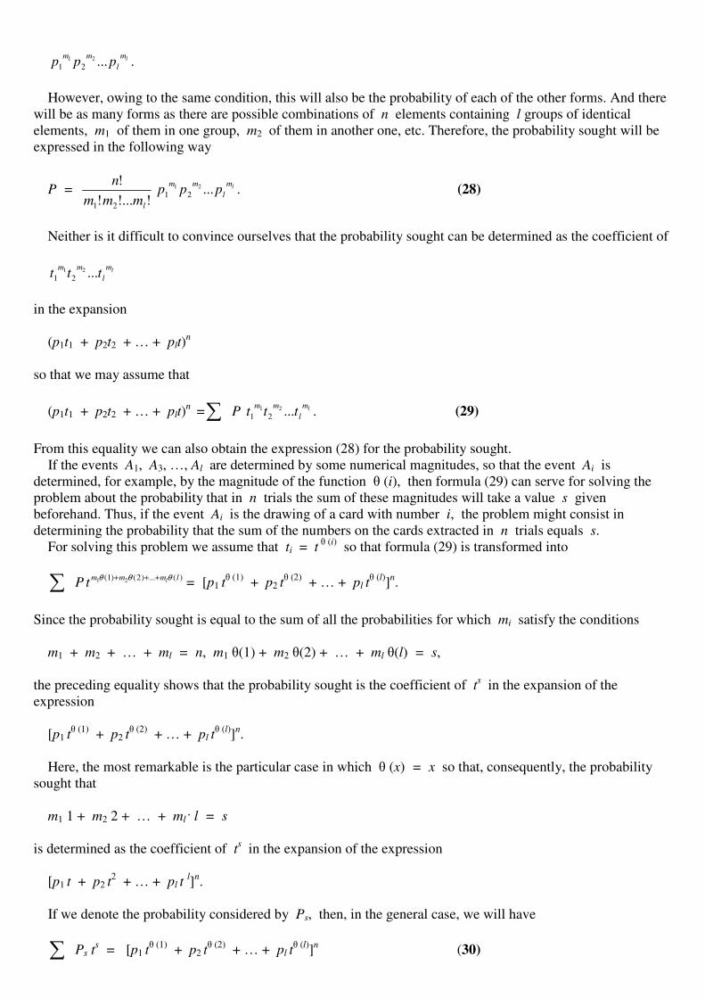
lm

l

mmppp ...21

21 .

However, owing to the same condition, this will also be the probability of each of the other forms. And there

will be as many forms as there are possible combinations of n elements containing l groups of identical

elements, m1 of them in one group, m2 of them in another one, etc. Therefore, the probability sought will be

expressed in the following way

P = !!...!

!

21 lmmm

nlm

l

mmppp ...21

21 . (28)

Neither is it difficult to convince ourselves that the probability sought can be determined as the coefficient of

lm

l

mmttt ...21

21

in the expansion

(p1t1 + p2t2 + … + plt)n

so that we may assume that

(p1t1 + p2t2 + … + plt)n

=� P lm

l

mmttt ...21

21 . (29)

From this equality we can also obtain the expression (28) for the probability sought.

If the events A1, A3, …, Al are determined by some numerical magnitudes, so that the event Ai is

determined, for example, by the magnitude of the function & (i), then formula (29) can serve for solving the

problem about the probability that in n trials the sum of these magnitudes will take a value s given

beforehand. Thus, if the event Ai is the drawing of a card with number i, the problem might consist in

determining the probability that the sum of the numbers on the cards extracted in n trials equals s.

For solving this problem we assume that ti = t & (i)

so that formula (29) is transformed into

� P)(...)2()1( 21 lmmm lt

θθθ +++= [p1 t

& (1) + p2 t

& (2) + … + pl t

& (l)]n.

Since the probability sought is equal to the sum of all the probabilities for which mi satisfy the conditions

m1 + m2 + … + ml = n, m1 &(1) + m2 &(2) + … + ml &(l) = s,

the preceding equality shows that the probability sought is the coefficient of ts in the expansion of the

expression

[p1 t& (1)

+ p2 t& (2)

+ … + pl t& (l)

]n.

Here, the most remarkable is the particular case in which & (x) = x so that, consequently, the probability

sought that

m1 1 + m2 2 + … + ml� l = s

is determined as the coefficient of ts in the expansion of the expression

[p1 t + p2 t2 + … + pl t

l]

n.

If we denote the probability considered by Ps, then, in the general case, we will have

� Ps ts = [p1 t

& (1) + p2 t

& (2) + … + pl t

& (l)]n (30)

whereas in the particular case indicated above this formula becomes

� Ps ts = [p1 t + p2 t

2 + … + pl t

l]

n. (xxii)

Suppose now that the events Ai are equally probable, i.e., that p1 = p2 = … = pl. Then pi = 1/l for any

i. In this case the formula derived (xxii) will be

� Ps ts = (t

n/l

n) [1 + t + t

2 + … + t

l–1]n =

(tn/l

n) [(t

l – 1)/(t – 1)]

n. (31)

Issuing from formula (31) we can indeed calculate the probability Ps that the sum of the magnitudes

determining the events occurring in n trials (in this case, the sum of the numbers corresponding to the events

taking place in these trials) is equal to a given magnitude s.

3.3.18. We shall now show how to obtain, when issuing from formula (31), the expression for the probability

Ps as some series. The problem is reduced to the determination of the coefficient of ts–n

in the expansion of

the expression

(tl – 1)

n/(t – 1)]

–n (xxiii)

in powers of t. But we have

(tl – 1)

n = t

ln – (n/1!) t

l (n–1) + [n(n – 1)/2!] t

l (n–2) – …, (xxiv)

(t – 1)]–n

= t –n

+ (n/1!) t –n–1

+ [n(n + 1)/2!] t –n–2

+ … +

[n (n + 1) … (n + , – 1)/,!] t –n–, + … (xxv)

Denoting l(n – i) – (n + ,) = s – n we obtain , = l(n – i) – s. Inserting this value of , in the

expression for the general term of the series (xxv) and making i consecutively equal to 0, 1, 2, … we will

obtain in this expansion all the possible terms, which, being multiplied by the first, the second, the third, …

term of the series (xxiv), will provide terms including ts–n

. We thus multiply the term number i in (xxv) by

the (i + 1)-th term in (xxiv).

It is seen now that the sum of the terms of the product of (xxiv) and (xxv) containing ts–n

will have the form

ts–n � (– 1)

i

!

)1)...(1(

i

innn +−−4

]!)([

]1)()...[1(

sinl

sinlnnn

−−

−−−++

where we ought to take all the values of i from 0 to n inclusively although under the conditions that the first

factor be replaced by 1 at i = 0 and the second factor, by 1 at i = (nl – s)/l and by 0 at larger values of

i. It ought to be remarked that nl is the maximal value that s can take; this follows from the fact that the sum

of the numbers {on the cards} cannot exceed the maximal number {on a card} taken as many times as there

were trials. On the grounds of the above, we conclude that the probability sought can be represented as

Ps = (1/ln)�

=

K

i 0

(– 1)i

!

)1)...(1(

i

innn +−−

]!)([

]1)()...[1(

sinl

sinlnnn

−−

−−−++ (32)

with

K = E [(nl – s)/l] + 1.

Issuing from here, we find the following expression for the probability Ps in the form of a series

Ps = (1/ln) {

)!(

)1)...(1(

sn

snlnnn

−

−−++ – Cn

1

]!)1([

)1)1()...[1(

snl

snlnnn

−−

−−−++

+ Cn2

]!)2([

]1)2()...[1(

snl

snlnnn

−−

−−−++ –

Cn3

]!)3([

]1)3()...[1(

snl

snlnnn

−−

−−−++ + …}

which breaks off as soon as we arrive at a term equal to 1 or 0.

To illustrate, we shall apply this conclusion to dice playing. This {particular} game consists in throwing six

dice having the form of cubes {of a cube}; numbers 1, 2, …, 6 are cut in their faces and the gain or loss

according to the condition of the game depends on the sum of the numbers turned up. Since it makes no

difference whether to throw one die six times or to toss six identical dice only once, we may consider the

throwing of each die as a trial so that in the case under consideration n = 6.

The number appearing on the upper face of the fallen die may be assumed to be the magnitude measuring the

event taking place in some {in the corresponding} trial, so that it is seen that here l = 6. Let us determine

now the probability Ps that the sum of the appeared numbers is s. In the case under consideration formula

(32) becomes

Ps = (1/66)�

=

K

i 0

(– 1)i

!

)7...(56

i

i−⋅�

)!636(

)641...(876

si

si

−−

−−⋅⋅

(33)

with K = E [(36 – s)/6] + 1. The magnitude s cannot exceed 36. Formula (33) provides P36 = 1/66 =

1/46 656. For s = 35 and 34, K = 1 in both cases and P = (1/66)46 = 1/7776 and (1/6

6)4647/2 =

(7/2)4(1/7776) = 7/15 552 respectively.

In the same way we find that

P33 = 2552 15

87

⋅

⋅ = 7/5832; P32 =

45832

97

⋅

⋅ = 7/2592;

P31 = 52592

107

⋅

⋅ = 7/1296; …

Supposing now that s = 30 we have K = E [(36 – 30)/6] + 1 = 2 and

P30 = 61296

117

⋅

⋅ –

66

6 = (1/7776) (77 – 1) = 19/1944, …

We see thus that the probability Ps increases with a decreasing s. It is not difficult to confirm that

P36 = P6; P35 = P7; P34 = P9 etc. (34)

Therefore, the probability Ps increases with an increasing s beginning with s = 6 and this increase

continues until s does not take the mean value between 6 and 36, i.e., until s = 21. And so, P21 is the

maximum of Ps. At s = 21 K = E [(36 – 21)/6] + 1 = 2 + 1 = 3. Therefore

P21 = (1/66)�

=

3

0i

(– 1)i

!

)7( 56

i

i−⋅

)!615(

)620...(876

i

i

−

−⋅⋅ =

(1/6

6) {

!15

201918...876 ⋅⋅⋅⋅ – 6

!9

14...876 ⋅⋅ +

21

56

⋅

⋅4

!3

876 ⋅⋅} =

66

875314131161917163 ⋅⋅⋅+⋅⋅⋅−⋅⋅⋅ = 4332/6

6 = 361/2592.

We have written the equalities (34) as though they were obvious but we shall prove them analytically. To

this aim, we shall represent the formula expressing Ps in a somewhat different form. We have the formula {cf.

(31)}

� Ps ts = (t

n /l

n)

nl

t

t���

����

�

−

−

1

1 (xxvi)

and, consequently,

� Ps ts = (1/l

n)4t n� (1 – t

l)

n4(1 – t) –n

=

(1/l n) t

n [1 – Cn

1 t

l + Cn

2 t

2l – … + (– 1)

i Cn

i t

il + …]4

{1 + nt + [n(n + 1)/2!]t2 + … + [n(n + 1)…(n + , – 1)/,!] t, + …}.

Denoting now , + il = s – n so that , = s – n – il, we obtain the following expression for the

general term of the coefficient of ts–n

:

(– 1)i Cn

i

)!(

)1)...(1(

nils

ilsnn

−−

−−+.

The coefficient itself will therefore be the sum of such expressions where i takes all the values from 0 to a

value (not inclusively) at which (s – n – il) becomes negative, i.e., to

i = E [(s – n)/l] + 1 = H.

However, Cni at i = 0, and the fraction at (s – n – il) = 0 should be replaced by unities. Under this

condition we obtain

Ps = (1/ln)�

=

H

i 0

(– 1)i Cn

i

)!(

)1)...(1(

nils

ilsnn

−−

−−+. (35)

When applying this formula to the game of dice we shall reduce it to the following form

Ps = (1/66)�

=

G

i 0

(– 1)i

!

)7...(56

i

i−⋅

)!66(

)16...(876

−−

−−⋅⋅

is

is

with G = E [(s – 6)/6] + 1. Substituting now s = 36 – k into formula (33) we obtain

P36–k = (1/66) �

+

=

1]6/[ E

0

k

i

(– 1)i

!

)7...(56

i

i−⋅

)!6(

)65...(876

ik

ik

−

−+⋅⋅.

When however assuming that s = 6 + k in formula (34), we get an identical expression and it is seen now

that indeed P36–k = P6+k. This, however, is a particular case of a general theorem because, when issuing from

formulas (32) and (35), it is not difficult to prove that, in general, Pln–k = Pn+k. And so, we find that

P6 = P36 = = (1/66) = 1/46 656; P7 = P35 = (6/6

6) = 1/7776;

P8 = P34 = (21/66) = 7/15 552; P9 = P33 = (56/6

6) = 7/5832; …;

P21 = 361/2592.

Let us study now several versions of a lottery where gains depend on the appearance of some sums of

numbers when tossing six dice. We have approximately

P6 = P36 = 1/46 656; P7 = P35 = 1/7776; P8 = P34 = 1/2222; …

Suppose now that the lottery is such that a gain of 46 656 corresponds to the sums equal to 6 and 36; a gain

of 7776 to sums 7 and 35; and a gain of 2222, to the sums 8 and 34, and assume also that no gains are

attached to the other sums. This version of the lottery can be described by the following table (Table 1). It is

seen that the expectation {of gain} in this lottery is 6; therefore, if desiring that it is fair, it is necessary that

the stake be equal to 6. Usually {however} it is 10

Table 1

Probabilities of gains Gains Expectations

P6 = 1/46 656 46 656 1

P7 = 1/7776 7776 1

P8 = 1/2222 2222 1

P34 = 1/2222 2222 1

P35 = 1/7776 7776 1

P36 = 1/46 656 46 656 1

Table 2

Probabilities Gains in lotteries (rubles)

of gains No. 1 No. 2 No. 3

P6 and P36 7776 11 664 23 328

P7 and P35 1296 1944 0

P8 and P34 370.3 0 0

copecks so that for being fair the gains in the lottery corresponding to the sums 6 and 36, 7 and 35, and 8

and 34 should be

(46 656/600)410 = 777.6 rubles; (7776/600)410 = 129.6r;

(2222/600)410 = 37.0r respectively

or, roughly, 780; 130; and 40 rubles.

Actually, however, the person licensed to organize a lottery assigns far lower gains so that the lottery is

profitable for him and very disadvantageous for its participants. Thus, instead of the 780, 130 and 40r, 78,

13 and 4r were for example assigned so that 9/10 of the stakes went to the organizer. Suchlike lotteries were

therefore abolished in every nation.

Let us compare now three lotteries: the first one, as described above; another lottery which includes four

gains, two of 46 656r each and two other ones of 7776r each; and a third one with {only} two gains of 46

656r each. We assume that the lotteries are fair. The expectation {of gain} in the first lottery, as we have seen,

is 6. For the second lottery, it is 4; and the expectation in the third lottery is 2. Supposing that the stakes are

identical and equal to 1r, we obtain the following comparative table (Table 2) for these lotteries.

We see that the gains in these {improved} lotteries considerably differ one from another. The largest ones

are in the lottery having the least number of gains, and although the probability of winning at least something is

different for each lottery, all of them are equally fair because the expectations are the same and {moreover}

equal to the stake1.

Note 1. {According to Buffon’s reasonable advice, a layman should rather ignore low probabilities (of gain)

regarding them as non-existent. The same conclusion follows from the concept of moral certainty (of loss)

which goes back to Descartes, Huygens and Jakob Bernoulli.}

3.3.19. Let us now consider the case in which l in formula (31) becomes very large and finally goes to

infinity, that is, the case in which we are engaged when determining the probability that a sum of a very large

or an infinite number of quantities having identical probabilities has a given value. We have {cf. (31)}

� Ps ts = (t

n/l

n) [(t

l – 1)

n/(t – 1)]

n. (xxvii)

We know however that if a function f (t) can be expanded into a series

Ao + A1 t + A2 t2 + … + AN t

N + …

then

AN = (1/2%) �−

π

π

f (e*i

) e–N*i

d*.

Therefore, denoting the right side of (xxvii) by f (t), we shall find {since Ps = As} that

ln PN = (1/2%) �

−

π

π

e*i (n–N)

n

i

il

e

e���

����

�

−

−

1

1

ϕ

ϕ

d*.

Noting now that

n

i

il

e

e���

����

�

−

−

1

1

ϕ

ϕ

= e (n/2) (l–1)* i

n

l���

����

�

/2)( sin

)2/( sin

ϕ

ϕ

we will find that

PN = (1/2%) �−

π

π

exp {[2

)1( −ln – N] * i}

n

l

l���

����

�

)2/sin(

)2/sin(

ϕ

ϕd*.

But

exp {[2

)1( −ln – N] * i} = cos {[

2

)1( −ln – N] *} +

i sin {[2

)1( −ln – N] *}

and consequently

PN = (1/2%) �π

0

cos {[2

)1( −ln – N] *}

n

l

l���

����

�

)2/sin(

)2/sin(

ϕ

ϕd*.

Substituting however l*/2 = & we obtain

PN = (1/%) �2/

0

lπ

cos {[2

)1( −ln – N] (2&/l)}

n

ll ���

����

�

)/( sin

sin

θ

θ(2/l) d&. (36)

The probability PN is thus expressed by a definite integral. Comparing this formula with formulas (32) amd

(35) we can calculate the value of the integral

�2/

0

lπ

cos {[2

)1( −ln – N] (2&/l)}

n

l ���

����

�

)/( sin

sin

θ

θd&.

We shall now search for the probability that N is contained within boundaries N1 and N2. Calling this

probability �, we obtain

∏2

1

N

N

=�2

1

N

N

PN =

(1/%) �2/

0

lπ

�2

1

N

N

cos {[2

)1( −ln – N] (2&/l)}

n

ll ���

����

�

)/( sin

sin

θ

θ(2/l) d&.

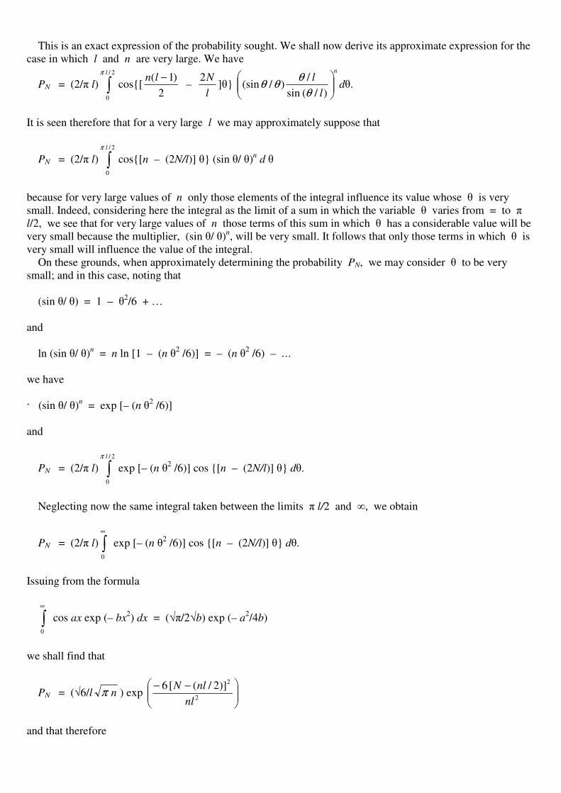
This is an exact expression of the probability sought. We shall now derive its approximate expression for the

case in which l and n are very large. We have

PN = (2/% l) �2/

0

lπ

cos{[2

)1( −ln –

l

N2]&}

n

l

l���

����

�

)/( sin

/)/(sin

θ

θθθ d&.

It is seen therefore that for a very large l we may approximately suppose that

PN = (2/% l) �2/

0

lπ

cos{[n – (2N/l)] &} (sin &/ &)n d &

because for very large values of n only those elements of the integral influence its value whose & is very

small. Indeed, considering here the integral as the limit of a sum in which the variable & varies from = to %

l/2, we see that for very large values of n those terms of this sum in which & has a considerable value will be

very small because the multiplier, (sin &/ &)n, will be very small. It follows that only those terms in which & is

very small will influence the value of the integral.

On these grounds, when approximately determining the probability PN, we may consider & to be very

small; and in this case, noting that

(sin &/ &) = 1 – &2/6 + …

and

ln (sin &/ &)n = n ln [1 – (n &2

/6)] = – (n &2 /6) – …

we have

4 (sin &/ &)n = exp [– (n &2

/6)]

and

PN = (2/% l) �2/

0

lπ

exp [– (n &2 /6)] cos {[n – (2N/l)] &} d&.

Neglecting now the same integral taken between the limits % l/2 and $, we obtain

PN = (2/% l) �∞

0

exp [– (n &2 /6)] cos {[n – (2N/l)] &} d&.

Issuing from the formula

�∞

0

cos ax exp (– bx2) dx = (#%/2#b) exp (– a

2/4b)

we shall find that

PN = (#6/l n π ) exp ���

����

� −−2

2)]2/([ 6

nl

nlN

and that therefore

∏2

1

N

N

=�2

1

N

N

(#6/l n π ) exp ���

����

� −−2

2)]2/([ 6

nl

nlN.

Expressing this sum through an integral, as we also did before, and noting that for very large values of n all

the terms except for the integral {?} will be very small, we may assume that

∏2

1

N

N

= (#6/l n π ) �2

1

N

N

exp ���

����

� −−2

2)]2/([ 6

nl

nlNdN.

Substituting now (#6/l�n) [N – (nl/2)] = t, we will obtain

∏2

1

N

N

= (1/#%) �2

1

t

t

exp (– t2) dt (37)

where

t1 = (#6/l#n) [N1 – (nl/2)], t2 = (#6/l#n) [N2 – (nl/2)].

Especially remarkable is the case in which t1 = – u, t2 = u, so that

� = (2/#%) �u

0

exp (– t2) dt. (38)

It is seen now that it is very probable that N satisfies the inequalities

(nl/2) + (l#n/#6) u > N > (nl/2) – (l#n/#6) u

or

(l/2) + (lu/ n6 ) > N/n > (l/2) – (lu/ n6 ). (39)

Here, N is the sum of the values of all the events {cf. §3.3.17} occurring in n trials and we know that only

one of these events can take place in any separate trial and that, on the other hand, one of them certainly ought

to occur in each trial.

The formula (38) therefore determines the probability that the arithmetic mean of a very large number of

magnitudes having equal probabilities of taking place in a very large number of trials is contained within the

boundaries

(l/2) + (lu/ n6 ), (l/2) – (lu/ n6 ).

Since this probability can be made arbitrarily close to 1, we might say that

lim (N/n) n = $ = l/2,

i.e., that the arithmetic mean of a very large number of quantities having equal probabilities tends to the limit,

as the number of trials increases to infinity, equal to half the number of all the quantities; or, to half of the

maximal quantity.

When desiring to solve the problem of whether an event is random or should it be attributed to certain

causes, scientists base some of their physico-mathematical investigations on the conclusion to which we have

arrived.

Suppose that event Ai is measured by magnitude ih so that the events under consideration have

magnitudes h, 2h, …, lh with lh being their maximal value which we shall denote by a. Multiplying the

inequality (39) by h we have

(a/2) + (au/ n6 ) > hN/n > (a/2) – (au/ n6 ).

It is seen now that at n = $ the arithmetic mean of all the magnitudes, hN/n, has half of the maximal one

of them, a/2, as its limit. Let us apply this result to a problem in astronomy. If the inclinations of the planes of

the planetary orbits to the plane of the ecliptic were absolutely random; in other words, if the probability that

the inclination & did not depend on &, we would have found that the arithmetic mean of all the inclinations

approximately equalled 90° (one half of the maximal inclination, of 180°), i.e., the mean plane of the

planetary orbits would have been perpendicular to the plane of the ecliptic. It occurs however that the planetary

orbits make very small angles with the ecliptic so that the arithmetic mean of all the inclinations very little

differs from zero. On these grounds it is concluded that the inclination of the planetary orbits is not

{inclinations are not} random; that there existed some causes which imparted an approximately the same small

inclination to all of them1.

Note 1. {See a description of the pertinent work of Laplace in my paper (Arch. Hist. Ex. Sci., vol. 9, 1973).}

3.3.20. Let us go over to a new and the last issue of the theory of probability. Although it does not concern

repetitions of events, we insert it in this section because it is very closely linked with the problem considered in

§3.3.19.

And so, we are going over to the determination of the probability that a sum of quantities varying due to

random causes is contained within given boundaries. Suppose that we have several quantities x, y, z, etc, and

assume that x can only have the values x1, x2, …; y, only the values y1, y2, …; z, only the values z1, z2,

…

Denote the probabilities that x has value xi, by pi; that y has value yi, by qi; that z has value zi, by

ri; etc. It is assumed that x, y, z, etc certainly have one of their values as stipulated above, so that

p1 + p2 + … = 1, q1 + q2 + … = 1, r1 + r2 + … = 1.

Then, let

p1 x1 + p2 x2 + … = a, q1 y1 + q2 y2 + … = b, r1 z1 + r2 z2 + … = c;

p1 x12 + p2 x2

2 + … = a1, q1 y1

2 + q2 y2

2 + … = b1,

r1 z12 + r2 z2

2 + … = c1 (40)

so that a, b, c, … are the expectations of the {considered} quantities, and a1, b1, c1, … the expectations of

their squares. Let us now search for the probability that

x + y + z + … = s.

It is not difficult to see that if the probability sought is Ps, then

� Ps ts = ( )...21

21 ++ xxtptp 4 ( )...21

21 ++ yytqtq 4 ( )...21

21 ++ zztrtr … (41)

Now, so as to simplify the derivation, we suppose that x, y, z, … can only have integer values. Later on, it

will be possible to remove this restriction by assuming that these quantities are expressed in very small

fractions of that unit in which we suppose them to be expressed during our deductions. Of course, such an

approach presumes that x, y, z, … are rational quantities, whereas, for a general solution of our problem, we

ought to assume them as arbitrary quantities. Nevertheless, we adopt our restriction because we shall only

search for an approximate value of the probability Ps.

Under the restrictions made we shall find that

Ps = (1/2%) �−

π

π

[p1 exp (x1*i) + p2 exp (x2*i) + …]4

[q1 exp (y1*i) + q2 exp (y2*i) + …]4[r1 exp (z1*i) + r2 exp (z2*i) + …]4 e

–s*i d*.

We shall now make approximate conclusions supposing that the number of the quantities x, y, z, … is very

large. Guiding ourselves by the considerations developed in §3.3.16, we may, when approximately calculating

this integral, neglect the powers of * exceeding the second one. Consequently, noting that

p1 exp (x1*i) + p2 exp (x2*i) + … = p1 {1 + [(x1*i)/1!] –

[(x12*2

)/2!] + …} + p2 {1 + [(x2*i)/1!] – [(x22*2

)/2!] + …} + …,

we obtain, on the strength of the equalities (40),

Ps = (1/2%) �−

π

π

[1 + a*i – (a1*2)/2]4 [1 + b*i – (b1*

2)/2]4

[1 + c*i – (c1*2)/2]… e

–s*i d*.

But we have

ln {[1 + a*i – (a1*2)/2]4 [1 + b*i – (b1*

2)/2]…} =

a*i – (a1*2)/2 – (1/2) [a*i – (a1*

2)/2]

2 + …

b*i – (b1*2)/2 – (1/2) [b*i – (b1*

2)/2]

2 + … = (a + b + c) *i +

[(a2 – a1) + (b

2 – b1) + (c

2 – c1) + …] (*2

/2) = A *i – B(*2/2)

where

a + b + c + … = A, – [(a2 – a1) + (b

2 – b1) + (c

2 – c1) +…] = B

(xxviii)

We thus get

Ps = (1/2%) �−

π

π

exp [– B(*2/2)] exp (A*i) exp (– s*i) d* =

(1/%) �π

0

exp [– B(*2/2)] cos [(A – s) *] d*.

Neglecting the magnitude of the last integral taken within % and $, which is allowable for sufficiently

large and positive values of B, we arrive at

Ps = (1/%) �∞

0

exp [– B(*2/2)] cos [(A – s) *] d* =

Bπ2

1exp [– (A – s)

2/2B]. (42)

In order to justify the approximation made just above, it ought to be proved that B > 0 and that, when the

number of the quantities x, y, z, … increases, B increases as well. To this end, it is sufficient to prove that all

the magnitudes

(a1 – a2), (b1 – b

2), … are positive. Let us take one of these differences, and what will be said about it will

also hold for the other ones. We have

a1 – a2

= a1 – 2a2

+ a2 = p1x1

2 + p2x2

2 +… – 2a (p1x1 + p2x2 +…) +

a2(p1 + p2 + …) = p1(x1

2 – 2ax1 + a

2) + p2(x2

2 – 2ax2 + a

2) + … + =

p1(x1 – a)

2 + p2(x2

– a)

2 + …

This shows that the magnitude (a1 – a2) is always positive.

We turn now to formula (42) that determines the probability Ps that the sum (x + y + z + …) has a

given value s. Denoting the probability that s is contained within the boundaries so and s1 by � and

noting that in virtue of our assumption B is very large, so that the sum might be without a perceptive error

replaced by an integral, we obtain

� = �1

0

s

s

Ps ds. (xxix)

where Ps is given by expression (42).

Considering this formula, we note that it determines the probability in the form of a homogeneous function

of degree zero with respect to the quantities x, y, z, … Therefore, it will not change if we change the unit in

which these quantities are expressed. Consequently, the adopted restriction concerning these quantities may be

abandoned and we shall now suppose that s in the formula (xxviii) is arbitrary1.

Denoting now

[(s – A)/ B2 ] = t, so = A + to B2 , s1 = A + t1 B2

we obtain

∏+

+

BtA

BtA

2

2

1

0

= (1/#%) �1

0

t

t

exp (– t2) dt.

If to = – u and t1 = u we get

∏+

−

BuA

BuA

2

2

= (2/#%) �u

0

exp (– t2) dt. (43)

This is the formula that indeed determines the probability that

A + u B2 > s > A – u B2

with A and B introduced in formulas (xxviii). This probability tends to 1 with an increasing u, but, on the

other hand, the interval between the boundaries for s will {then} become wider. These boundaries depend also

on the magnitude B, which, in turn, depends on the number of the quantities x, y, z, … Denoting this number

by n, we find that the formula (43) determines the probability that

(A/n) – (u/#n) nB /2 < s/n < (A/n) + (u/#n) nB /2 .

We have already obtained these inequalities and their probability in §§3.2.1 and 3.2.2 where it was shown that

∏+

−

BuA

BuA

2

2

= 1 – (&/2u2) (xxx)

where & was a proper fraction. Formula (xxx) was proved there absolutely rigorously 2. This formula ought to

be therefore applied in theoretical investigations although it does not allow the {actual} calculation of the

probability. Formula (43) that provides such a possibility was however derived in a non-rigorous way. The lack

of rigor in the derivation consisted in that we made various assumptions without determining the boundary of

the ensuing errors. In its present state, mathematical analysis cannot derive this boundary in any satisfactory

fashion 3. In spite of this, we shall apply formula (43) when expounding the method of least squares to which

we are now indeed going over.

Note 1. This already follows from the replacement of the sum by an integral so that ds was introduced

assuming that s varied continuously.

Note 2. Formula (xxx) can be obtained by substituting t = u#2 in the final formula of §3.2.1.

Note 3. Liapunov […] provided quite a rigorous general proof of this so-called {central} “limit theorem of

the theory of probability”. It is possible that the preceding words of his celebrated teacher had indeed prompted

him to consider this problem. A. Krylov.

3.4. Applications of the Theory of Probability to the Treatment of

Observations

3.4.1. In the sequel, we shall base our considerations on formula (43) that determines the probability that the

sum (x + y + z + …) of quantities varying due to random circumstances is contained within the boundaries

A + u B2 and A – u B2 .

We shall choose such a value for u that this probability determined by the formula

(2/#%) �u

0

exp (– t2) dt (xxxi)

will be equal to 1/2. This value is approximately 0.48. In this case, we shall call the boundaries indicated

above probable because the probable boundaries for the sum (x + y + z + …) are such that it is contained

with equal probability either within or beyond them. The “width” of these boundaries is approximately

240.48 B2 = 0.96 B2 . We know however that for somewhat considerable values of u, for example for u

= 3, the magnitude (xxxi) is very close to 1 1; therefore, if the “width” of the probable boundaries be

increased six- or seven-fold, we shall already obtain such boundaries for which we may say with a very high

probability that the sum (x + y + z + …) is contained within them.

When considering errors of observation, we shall call them probable if they are contained within probable

boundaries; that is, between the boundaries A – 0.48 B2 and A + 0.48 B2 , and we shall always

assume in the sequel that u = 0.48.

Before going ahead, let us agree about one more term; we shall say that the observations do not include a

“constant error” if positive and negative errors are equally probable, i.e., if the expectation of the errors is zero.

We shall assume that this condition is fulfilled; that is, we shall consider the expectation of the errors equal to

zero. If however we shall have to study observations corrupted by constant errors we shall make the

appropriate reservation. It ought to be noted that the equally probable errors are supposed to be those having

equal numerical values.

Note 1. For the sake of clearness we append a short table of the values of this integral {omitted}. A. Krylov.

3.4.2. Suppose that we are concerned with measuring some quantity V and that the observations provided

its following values: L1, L2, …, Ln. In this case their arithmetic mean, i.e., (L1 + L2 + … + Ln)/n, is usually

taken as the value of V; and, the larger is the number of observations, n, the closer we consider it to be to V.

We shall now show the grounds on which such opinions are based.

Let 71, 72, …, 7n be the errors of the first, the second, .., the n-th observation. We shall consider those

errors which increase the real value of V as positive and regard those that decrease it as negative. Under these

conditions we have

V = L1 – 71, V = L2 – 72, …, V = Ln – 7n (xxxii)

so that

nV = (L1 + L2 + … + Ln) – (71 + 72 + … + 7n),

V = [(L1 + L2 + … + Ln)/n] – [(71 + 72 + … + 7n)/n].

It is seen therefore that, when assuming the arithmetic mean of the observational values as V, we make an

error equal to

7 = (71 + 72 + … + 7n)/n.

Let us find the probable boundaries of this error. Applying formula (43) to this case, and denoting x = 71/n, y

= 72/n, z = 73/n, … we have in this case

a = (1/n)� 71(i) pi = 0; b = (1/n)� 72(i) qi = 0; …

where 71(i) is one of the possible errors of the first observation and pi, its probability; 72(i), one of the

possible errors of the second observation and qi, its probability, etc.

Consequently, we have A = a + b + c + … = 0. Then

a1 = � (71(i)/n)2 pi = (1/n

2) � (71(i))

2 pi = k/n

2

where

k = � (71(i))2

pi.

The value of k depends on the quality of the observations and it is not difficult to see that the less it is the

better are the observations because k can only be small when the errors are small in numerical value. If all the

observations are equally good, then k is the same for all of them and we will have

a1 = b1 = c1 = … = k/n2

so that

B = ( a1 – a2) + ( b1 – b

2) + ( c1 – c

2) + … = nk/n

2 = k/n.

We thus see that the magnitudes

–u nk /2 and u nk /2

will be the probable boundaries for 7. They show that the “width” of the probable boundaries decreases with

the increase in the number of observations provided that all of them are equally good. This indeed is the basis

for increasing this number when it is desired to determine the quantity sought “more precisely” through the

arithmetic mean of the observed values. Let us now go over to another issue.

3.4.3. Suppose that we are again concerned with determining the quantity V for which the observations

provided the values L1, L2, …, Ln. It is required to find such a combination of these observations as would

have furnished the most probable value of V. This problem can be formulated either as finding the best

combination out of all the possible ones; or, out of all combinations of a given form.

In the first case, the problem is of course much more general, and it can only be solved by applying the law

of hypotheses 1 whereas no deductions made on its basis have adequate rigor. We shall therefore solve this

problem in its second version choosing the following form of the combinations

(,1L1 + ,2L2 + … + ,nLn)/( ,1 + ,2 + … + ,n). (xxxiii)

Here, we shall try to determine ,1, ,2, …, ,n in conformity with the condition that this combination expresses

V in the best way, i.e., that the probable boundaries of the error be the tightest {the narrowest}. Note that the

arithmetic mean is a particular case of this combination; namely, the case in which ,1 = ,2 = … = ,n.

From equalities (xxxii) {multiplying them by ,i respectively, etc} we have

V (,1 + ,2 + … + ,n) = (,1L1 + ,2L2 + … + ,nLn) –

(71,1 + 72,2 + … + 7n ,n),

V = [(,1L1 + ,2L2 + … + ,nLn)/ (,1 + ,2 + … + ,n)] –

[(71,1 + 72,2 + … + 7n,n)/ (,1 + ,2 + … + ,n)]

so that, when assuming the quantity (xxxiii) as V, we make an error equal to

7 = (71,1 + 72,2 + … + 7n,n)/ (,1 + ,2 + … + ,n).

We shall now find the probable boundaries of this error. Let

x = nλλλ

λε

+++ ...21

11 , y = nλλλ

λε

+++ ...21

22 , z = 321

33

... λλλ

λε

+++ etc.

In this case we have

a =�n

i

λλλ

λε

+++ ...21

1)(1pi =

nλλλ

λ

+++ ...21

1 � 71(i) pi = 0

so that a = b = c = … = 0 and, consequently, A = 0. We then have

a1 =� 2

21

2

1

2

)(1

)...(

)(

n

i

λλλ

λε

+++pi = [

nλλλ

λ

+++ ...21

1 ] 2 � (71(i))2 pi =

k [nλλλ

λ

+++ ...21

1 ] 2 .

Supposing that all the observations are equally good, we obtain, in an absolutely similar way,

b1 = 2

21

2

2

)...( n

k

λλλ

λ

+++, c1 =

2

21

2

3

)...( n

k

λλλ

λ

+++, …

and therefore

B = 2

21

22

2

2

1

)...(

)...(

n

nk

λλλ

λλλ

+++

+++.

so that the probable boundaries are

– u B2 , u B2 .

As already stated, the best combination is that for which the “width” of the boundaries is least so that the

problem is reduced to the determination of ,1, ,2, …, ,n in accord with the condition that the expression

W = (,12 + ,2

2 + … + ,n

2) /( ,1 + , + … + ,n)

2 (xxxiv)

is minimal.

It is easy to see however that in such a form the problem is indefinite because the magnitudes ,1, ,2, …, ,n

themselves will not thus be determined, only the ratios between them will be derived. We may therefore lay

down any {additional} condition between them {connecting them} expressed by one equation. The simplest

result will be provided by stipulating that

,1 + , + … + ,n = 1 (44)

so that

W = ,12 + ,2

2 + … + ,n

2. (xxxv)

The condition that W be minimal furnishes the equations

,1 d,1 + ,2 d,2

+ … + ,n d,n = 0, d,1

+ d,2

+ … + d,n = 0.

Multiplying the second one by an indefinite factor 2, subtracting {the product} from the first one and equating

then the coefficients of d,1, d,2, …, d,n to zero, we obtain

,1 = 2, ,2

= 2, …, ,n

= 2.

Together with equation (44) these equations provide

,1 = ,2

= … = ,n

= (1/n).

We thus see that the minimum of W takes place when the magnitudes ,1, ,2, … , ,n are equal one to

another.

It is not amiss to derive this {the same result} in another, elementary way. Suppose that

,1 + ,2

+ … + ,n

= s.

We have

[,1 – (s/n)]

2 + [,2

– (s/n)]

2 + … + [,n

– (s/n)]

2 =

,12 + ,2

2 + … + ,n

2 – 2(s/n) (,1

+ ,2

+ … + ,n) + (ns

2/n

2)

so that

,12 + ,2

2 + … + ,n

2 = (s

2/n) +

[,1 – (s/n)]

2 + [,2

– (s/n)]

2 + … + [,n

– (s/n)]

2

and consequently 2

W = (1/n) + {[,1 – (s/n)]

2 + [,2

– (s/n)]

2 + … + [,n

– (s/n)]

2}/s

2.

Since the second term on the right side of this equality is always positive, we see that the minimum of W

will only take place when this term vanishes; that is, when

,1 = ,2

= … = ,n

= (s/n)

or, in accord with the condition that the magnitudes ,1, ,2, …, ,n are equal one to another. We thus conclude

that the magnitude (L1 + L2 + … + Ln)/n,

and the arithmetic mean of the observed magnitudes, ought to be taken as V.

Note 1. {Chebyshev did not use this term in the relevant sections (§§3.1.6 – 3.1.7) but he obviously thought

here about the Bayesian approach with an arbitrary choice of the prior distribution. In §3.4.9 he wrongly

attributed to Gauss the justification of the method of least squares by this law of hypotheses. However, the

postulate of the arithmetic mean adopted by Gauss in 1809 made the Bayesian approach superfluous;

E.T.Whittaker & G. Robinson (Calculus of Observations. London, 1924, p. 219n) were the first to indicate this

point (overlooked by Gauss), and even their remark was forgotten. Also note that Gauss subsequently

abandoned his initial substantiation of the method. In general, Chebyshev was poorly acquainted with the work

of the creator of the method of least squares as especially witnessed by his wrong reasoning in §3.4.9, see my

papers of 1994 in the Arch. Hist. Ex. Sci., vols 46 and 48.}

Note 2. {Chebyshev issues here from formula (xxxiv).}

3.4.4. Having shown that out of all the combinations of the type of (xxxiii) the best one is the arithmetic

mean of the observed magnitudes, we shall show now on what grounds should we search for the best of all the

possible combinations.

Suppose that we know the function * (7) determining the probability that the error has magnitude 7. In this

case we can easily determine the best combination of the observations. Indeed, let us assume that V can take

the values Vo, V1, V2, …, V,, … (which can be arbitrarily close one to another). In order to determine V we

made n observations providing the values L1, L2, …, Ln. This represents event E.

The various hypotheses under which this event can happen are V = Vo, V = V1, V = V2, …, V = V,,

… Knowing nothing about the appropriate probabilities, we suppose that they are equal one to another and we

denote their common value by P. Then Po = P1 = P2 = … = P, = … = P. This assumption is arbitrary

and none of the subsequent deductions is therefore rigorous. The probability of the event E under the

hypothesis that V = V,, i.e., that, when determining some quantity V, by observations, we got the values

L1, L2, …, Ln, is

p, = * (L1 – V,)4 * (L2 – V,) … * (Ln – V,).

Therefore, the probability that the event E took place under the hypothesis V = V, will be expressed in the

following way

� λλ

λλ

pP

pP = � −−−

−−−

)()...()(

)()...()(

21

21

λλλ

λλλ

ϕϕϕ

ϕϕϕ

VLVLVL

VLVLVL

n

n

where the sum is extended over all the values of , and is therefore a constant magnitude.

The search for the maximum of this probability is thus reduced to the search for the maximum of the

expression

W = * (L1 – V,)4 * (L2 – V,) … * (Ln – V,). (xxxvi)

In the case in which the function * (z) is known, this condition will indeed provide an equation for

determining V, as a function of the observed magnitudes L1, L2, …, Ln. This latter function will indeed

furnish the best combination of the observations because the probability that V, is equal to that combination is

maximal. We thus see that everything consists in determining the type of the function * (z). Some theoretical

considerations which we will discuss below lead to the conclusion that

* (z) = F exp (– gz2) (xxxvii)

where F and g are some constant magnitudes. Experimental corroboration of this formula was being

attempted and it was found out that (xxxvii) rather well expresses the law of the probability of error as a

function of the change in the value of this error.

Assuming the function (xxxvii) as * (z) we shall find that

W = F n exp (– gt

2),

t2 = (L1 – V,)

2 +4 (L2 – V,)

2 + … + (Ln – V,)

2. (xxxviii)

It is therefore seen that the maximum of W will take place when the right side of (xxxviii) where V, is

considered as the independent variable is maximal. The value of V, making the expression (xxxviii) maximal

is determined by the equation

– 2(L1 – V,) – 2(L2 – V,) – … – 2(Ln – V,) = 0

which provides

V, = (L1 + L2 + … + Ln)/n.

The assumption that * (z) is expressed by the formula (xxxvii) leads to the conclusion that the best of all the

possible combinations is the arithmetic mean of the observed magnitudes.

3.4.5. We shall now show on what theoretical grounds is the determination of the type of the function * (z)

founded. Note that when two observations are available it might be assumed as an obvious condition that their

best combination is the arithmetic mean because in this case nothing empowers us to prefer one of the observed

magnitudes to the other one. We therefore really ought to decide in favor of the magnitude which would be

equally distant from each of the observed magnitudes.

But the same can not be said about three or more observations. Indeed; suppose that we made three

observations and that two of them furnished one and the same value for the quantity sought, V. In such a case

we ought to prefer the magnitude which was repeated twice, but should our preference be expressed in taking

2/3 of the repeated magnitude and 1/3 of the magnitude that occurred {only} once, and in assuming that the

sum thus obtained is the quantity V? Obviously we have no right to assert this.

We shall now show that, if the arithmetic mean is taken as the best combination out of three observations, it

is possible to find the type of the function * (z). We saw that the best combination is found from the condition

of the maximum of the expression (xxxvi). For three observations this will be

W = * (L1 – V,)4* (L2 – V,)4* (L3 – V,).

The search for its maximum leads to equation

)(

)(

1

1

λ

λ

ϕ

ϕ

VL

VL

−

−′ +

)(

)(

2

2

λ

λ

ϕ

ϕ

VL

VL

−

−′ +

)(

)(

3

3

λ

λ

ϕ

ϕ

VL

VL

−

−′ = 0.

Denote *)(z)/* (z) = +(z), then this equation will take the form

+ (L1 – V,) + + (L2 – V,) + + (L3 – V,) = 0.

Now we ought to express the demand that this equation be satisfied if

V, = (L1 + L2 + L3)/3.

Assuming this value, we obviously have

(L1 – V,) + (L2 – V,) + (L3 – V,) = 0.

Therefore, denoting (L1 – V,) = y and (L2 – V,) = y1, we obtain

(L3 – V,) = – (y + y1)

so that we ought to have the equality

+ (y) + + (y1) + + [– (y + y1)] = 0 (45)

valid for any y and y1. We may thus consider it as an equation determining the function + (y).

Here we encounter a new mathematical problem: A function is determined not by a differential equation, not

by an equation in finite differences, but by an equation connecting the values of the function sought

corresponding to various values of the independent variables somehow connected one with another. Such

equations are called functional. Some mathematicians concerned themselves with their solution (Abel among

others), and some are engaged in this problem also at present. However, until now there exist no general

methods for solving them whereas the existing methods actually consist in that, out of a given functional

equation, a differential equation is made up by differentiation and elimination of the unknown magnitudes. We

shall show one of these methods while studying the particular case under consideration.

Differentiating the equation (45) with respect to y we find out that

+) (y) – +) (– y – y1) = 0.

Differentiating this equation, now with respect to y1, we get

+1 (– y – y1) = 0.

Denoting – y – y1 = z, we obtain +1 (z) = 0 so that

+ (z) = C z + C1.

Making use now of the determined type of the function + (z), we shall reduce the equation (45) to the form

C y + C1 + C y1 + C1 – C (– y – y1) + C1 = 0

so that C1 = 0. It follows that

+ (z) = C z = *)(z)/* (z)

and, consequently, that

(1/F) ln * (z) = C z2/2, * (z) = F exp (C z

2/2).

Therefore

W = F3 exp {(C/2) [(L1 – V,)

2 + (L2 – V,)

2 + (L3 – V,)

2]}

and

dW/dV, = CW [– (L1 – V,) – (L2 – V,) – (L3 – V,)],

d2W/dV,

2 = C (dW/dV,) [– (L1 – V,) – (L2 – V,) – (L3 – V,)] + 3CW.

Assuming that 3V = L1 + L2 + L3, we find that

d2W/dV,

2 = 3CW.

Since W, at the considered values of V,, should be maximal, the expression obtained for d2W/dV,

2 ought to

be negative. And since W is positive (as being a product of three positive multipliers), C is negative.

Therefore, denoting C = – 2g, we obtain (xxxvii) where F and g are some positive magnitudes.

Thus, assuming that the arithmetic mean is the best combination of three observations, we found the type of

the function * (z) . However, as we said already, this supposition is arbitrary and not caused by necessity.

Note that the assumption that the arithmetic mean is the best combination for two observations is necessary but

not sufficient for determining the type of the function * (z). Indeed, in this case the equation determining the

best combination will be

)(

)(

1

1

λ

λ

ϕ

ϕ

VL

VL

−

−′ +

)(

)(

2

2

λ

λ

ϕ

ϕ

VL

VL

−

−′ = 0.

Denoting as before *)(z)/* (z) = +(z) we shall reduce it to

+ (L1 – V,) + + (L2 – V,) = 0.

This equation should be satisfied by V, = (L1 + L2)/2; expressing this {condition} and denoting L1 + L2 =

2y, we obtain

+ (y) + + (– y) = 0.

This equation, however, does not determine the function + (y) because any odd function satisfies it.

If we assume that indeed (xxxvii) holds, we shall easily arrive at the method of least squares. To this end

denote the error of the i-th observation by xi. We have seen however that the probability of some totality of

errors is determined thus:

� )]( )...( )( [

)( )...( )(

21

21

n

n

xxx

xxx

ϕϕϕ

ϕϕϕ.

Therefore, we ought to assign such magnitudes to the errors 1 that the expression

* (x1)4* (x2) … * (xn) (47)

be maximal because the denominator in the preceding expression is a constant magnitude. Given the existence

of the equation above, this product will be

F n exp [– g(x1

2 + x2

2) + … + xn

2)].

Consequently, we should assign such values to the errors that the expression

x12 + x2

2 + … + xn

2

be minimal; that is, in order to find the most probable errors we ought to find the minimum of the sum of their

squares.

Note 1. {Chebyshev did not expressly distinguish between errors and residuals.}

3.4.6. Very often the observations directly provide not the quantity sought, V, but quantities connected with

it by some equations. We shall consider the case in which the observations furnish the quantities

'1V, '2V, …, 'nV.

Here, '1, '2, …, 'n are known numbers and �iV is a quantity determined by the i-th observation. Suppose

that for these quantities the n observations gave such values: L1, L2, …, Ln. the problem consists in finding

the most reliable magnitude for V. When solving this problem we will not search for the best of all the

possible combinations of the observations, because, as it was shown on a simpler case, this cannot be done in a

rigorous way. We will {rather} determine the most favorable combination out of those of the type

nn

nnLLL

αλαλαλ

λλλ

+++

+++

...

...

2211

2211 .

Denoting the error of the i-th observation by 7i, we have

a1V = L1. – 71, a2V = L2. – 72, …, anV = Ln. – 7n.

Multiplying these equations by �1, �2, …, �n respectively, and adding up the results, we obtain

(a1 �1 + a2 �2 + … + an �n) V =

(�1 L1 + �2 L2 + … + �n Ln) – (�1 71 + �2 72 + … + �n 7n)

and

V = nn

nnLLL

αλαλαλ

λλλ

+++

+++

...

...

2211

2211 – nn

nn

αλλαλ

ελελελ

+++

+++

...

...

211

2211 . (xl)

It is seen therefore that, when assuming formula (xxxix), we make an error equal to the second term on the

right side of (xl).

We shall now search for the probable boundaries for 7 and determine

�1, �2, …, �n from the condition that these boundaries are as close as possible to each other. However, if we do

not {additionally} lay down any condition concerning these magnitudes, the issue will be indefinite. We shall

therefore assume that

'1 �1 + '2 �2 + … + ' n �n = 1 (xl1)

from which the generality of the solution certainly will not suffer. And so, we have

V = �1 L1 + �2 L2 + … + �n Ln, 7 = �1 71 + �2 72 + … + �n 7n.

When determining the probable boundaries for 7, we shall apply formula (43). To this end we denote

x = �1 71, y = �2 72, z = �3 73, …

and we shall understand 71(i) as one of the possible values of 71, – that is, as one of the possible errors of the

first observation, – 72(i) as one of the possible values of 72, etc.

Supposing now that the observations have no constant errors, we have

a =� �1 71(i) pi = �1� 71(i) pi = 0, …, b = 0, c = 0, …

Assuming in addition that all the observations are of an equally high quality, we obtain

a1 = � [�1 71(i)]2 pi = �1

2� [71(i)]2 pi = �1

2 k

and, in the same way,

b1 = �22 k, c1 = �3

2 k, …

Thus, we find that

A = 0, B = k (�12 + �2

2 + … + �n

2).

The probable boundaries for 7 will be

– u B2 and u B2 .

The problem is now being reduced to the determination of the minimum of

�12 + �2

2 + … + �n

2

under the condition (xli). To this end, we derive the equation

(�1 – '1 2) d �1 + (�2 – '2 2) d �2 + … + (�n – 'n 2) d �n = 0

so that

�1 = '1 2, �2 = '2 2, …, �n = ' n 2.

Then, from equation (xli),

2 = 1/( '12

+ '22

+ … + 'n2)

and

�i = 22

2

2

1 ... n

i

ααα

α

++.

Consequently, the most reliable combination will be

V1 = 22

2

2

1

2211

...

...

n

nnLLL

ααα

ααα

+++

+++. (xlii)

If '1, '2, …, ' n are integers, it might be said about this expression of V, that, Supposing that we, after

making 'i2 observations, obtained in each of them the magnitude Li /' i for V; and supposing also that the

total number of observations was ('12

+ '22 + … + 'n

2), the best combination of the observations will be, as

we saw, the arithmetic mean of the observed values, hence (xlii).

The described method of determining V, expressed for the first time by Legendre, is indeed called the

method of least squares, – not because we search for the minimum of the sum of the squares of the factors �1,

�2, …, �n, but because, when applying it, the value of V imparts the minimal value, as we shall prove now,

to the sum of the squares of the errors.

To prove this, we shall find the value of V for which the sum

712 + 72

2 + … + 7n

2

becomes minimal. We have

712 + 72

2 + … + 7n

= (L1 – '1 V)

2 + (L2 – '2 V)

2 + … + (Ln – 'n V)

2.

For determining its minimum we obtain the equation

'1 (L1 – '1 V) + '2 (L2 – '2 V) + … + 'n (Ln – 'n V) = 0

from which we indeed arrive at (xlii)

Further on we shall expound the method of finding the best combinations for determining several unknowns

from observations; and we shall show that in this case as well the most reliable combinations are those for

which the sum of the squares of the errors is the least. We note right here that the method of least squares is not

the only one applied for the treatment of observations. There exists one more method according to which the

unknown quantity is determined from the observations in such a way that the maximal error is minimal and this

method is in some cases more advantageous than the method of least squares, but in general the latter should be

preferred.

3.4.7. Suppose now that it is required to determine from observations quantities U and V and that in the i-th

observation we search for the value of the expression ('iU + (iV) where 'i and (i are given numbers and

that this observation provides the magnitude Li. Denoting the error of the i-th observation by 7i, we have

'1U + (1V = L1 – 71, '2U + (2V = L2 – 72, …, 'nU + (nV = Ln – 7n.

(48)

We shall find the combinations by whose means U and V are determined with least errors. And, as before,

we shall only consider linear combinations (with respect to L1, L2, …). To this end we ought to proceed as

follows.

Multiply each of the equations (48) by some indefinite factor ,i and add up the results; this will provide one

equation for determining U and V, namely

('1,1 + '2,2 + … + 'n,n)U + ((1,1 + (2,2 + … + (n,n)V =

(L1,1 + L2,2 + … + Ln,n) – (71,1 + 72,2 + … + 7n,n).

We then subject the factors ,1, ,2, …, ,n to the conditions

'1,1 + '2,2 + … + 'n,n = 1, (1,1 + (2,2 + … + (n,n = 0. (49)

Consequently, we shall directly obtain an expression for U

U = (L1,1 + L2,2 + … + Ln,n) – (71,1 + 72,2 + … + 7n,n).

Knowing nothing about the magnitude of the errors, we assume for U the expression

U = L1,1 + L2,2 + … + Ln,n (50)

thus making an error equal to

7 = 71,1 + 72,2 + … + 7n,n. (51)

Had we subjected the factors to conditions

'1,1 + '2,2 + … + 'n,n = 0, (1,1 + (2,2 + … + (n,n = 1, (52)

we would have obtained an expression for V.

It is seen now that, after finding a final expression for U, we can directly write down a final expression for

V as well by replacing the letters 'i by (i and vice versa. We shall therefore only discuss now the

determination of U, and everything said about it will also apply to the determination of V.

And so, the issue is reduced to the determination of the best combination of the type

L1,1 + L2,2 + … + Ln,n

where ,1, ,2, …, ,n satisfy conditions (49) and we will indeed assume this best combination as U. To this

end let us find the probable boundaries for the error (51).

Denoting

k =� [71(i)]2 pi (53)

and supposing that all the observations are of an equally high quality, we shall find, as we did before, that these

boundaries are

– u )...(222

2

2

1 nk λλλ +++ , u )...(222

2

2

1 nk λλλ +++

so that everything is reduced to the determination of the minimum of the expression

�12 + �2

2 + … + �n

2 (xliii)

under the conditions (48). We have the equations

�1 d�1 + �2 d�2 + … + �n d�n = 0, '1d�1 + '2 d�2 + … + ' n d�n = 0,

(1 d�1 + (2 d�2 + … + (n d�n = 0.

Multiplying the second of these by – 2 and the third one by – A; adding up the results obtained with the

first equation; and equating the coefficients of

d�1, d�2, …, d�n to zero, we get equations of the type

�i = 'i 2 + (i A, i = 1, 2, …, n. (54)

For determining 2 and A we will have on the strength of (49) the equations

'1('1 2 + (1 A) + '2('2 2 + (2 A) + … + 'n('n 2 + (n A) = 1, (55a)

(1('1 2 + (1 A) + (2('2 2 + (2 A) + … + (n('n 2 + (n A) = 0, (55b)

or, in another form,

('12 + '2

2 + … + 'n

2) 2 + ('1(1 + '2(2 + … + 'n(n) A = 1, (56a)

('1(1 + '2(2 + … + 'n(n) 2 + ((12 + (2

2 + … + (n

2) A = 0. (56b)

Having determined 2 and A from these equations, we will find ,1, ,2, …, ,n from equations (54).

Consequently, we will also find both U and the probable boundaries of the error � if only we will know the

magnitude k whose determination is explained below.

We shall now show that the thus found value of U is identical with the one obtained from the condition of

minimum of the sum of the squares of the errors. We have

�1 = L1 – '1 U – (1 V, �2 = L2 – '2 U – (2 V, …,

�n = Ln – 'n U – (n V.

If we assume here that U and V are their real values, then �1, �2, …, �n will be constant magnitudes. We

will however consider them as variable quantities assigning to U and V not their real values, unknown to us,

but all possible variable values; and, among these, we will search for such that provide the minimum of

�12 + �2

2 + … + �n

2. (xliv)

We have

�12 + �2

2 + … + �n

2 = (L1 – '1 U – (1 V)

2 + (L2 – '2 U – (2 V)

2 +

… + (Ln – 'n U – (n V)2.

The condition of minimum of this sum leads to the equations

'1(L1 – '1 U – (1 V) + '2(L2 – '2 U – (2 V) + …

+ 'n(Ln – 'n U – (n V) = 0,

(1(L1 – '1 U – (1 V) + (2(L2 – '2 U – (2 V) + …

+ (n(Ln – 'n U – (n V) = 0

which are reduced to the form

('12 + '2

2 + … + 'n

2)U + ('1(1 + '2(2 + … + 'n(n)V =

'1L1 + '2L2 + … + 'nLn,

('1(1 + '2(2 + … + 'n(n)U + ((12 + (2

2 + … + (n

2)V =

(1L1 + (2L2 + … + (nLn.

Multiplying the first of these equations by 2, the second one by A, and adding up the results we get

U [('12 + '2

2 + … + 'n

2) 2 + ('1(1 + '2(2 + … + 'n(n) A] +

V [('1(1 + '2(2 + … + 'n(n) 2 + ((12 + (2

2 + … + (n

2) A] =

L1('12 + (1A) + L2('22 + (2A) + … + Ln('n2 + (nA).

Supposing now that 2 and A satisfy the equations (56) we will find that

U = L1('12 + (1A) + L2('22 + (2A) + … + Ln('n2 + (nA)

which coincides with the expression (50) if the factors ,1, ,2, …, ,n have the values (54) as found above. And

so, U and V determined by the best linear combination at the same time make the sum of the squares of the

errors minimal.

3.4.8. Let us now consider the general case. Suppose that it is required to determine from observations

quantities U, V, W, … whose number we will assume to be arbitrary. Suppose that we have the equations

'1U + (1V + 51W + … = L1 – 71, '2U + (2V + 52W + … = L2 – 72,

…, 'nU + (nV + 5nW + … = Ln – 7n, (57)

whose right sides are the directly observed magnitudes L1, L2, …, Ln; 71, 72, …, 7n are their errors whereas

'1, '2, …, 'n, (1, (2, …, (n, 51, 52, …, 5n, … are given numbers not depending on the observations and not

exposed to error. Let us take a number of factors

,1, ,2, …, ,n (xlv)

and subject them to conditions

'1,1 + '2,2 + … + 'n,n = 1, (1,1 + (2,2 + … + (n,n = 0,

51,1 + 52,2 + … + 5n,n = 0, … (58)

We multiply the equations (57) by ,1, ,2, … respectively; adding up the results obtained we get, in virtue of

these equations,

U = L1,1 + L2,2 + … + Ln,n – (71,1 + 72,2 + … + 7n,n),

an equation which we will write as

U =� Li,i –� 7i,i.

It is seen therefore that, when assuming the expression

L1,1 + L2,2 + … + Ln,n =� Li,i (59)

as U, we make an error equal to

7 = 71,1 + 72,2 + … + 7n,n =� 7i,i. (60)

In order to find probable boundaries of this error we assume, as we did before, that all the n observations

are of an equally high quality and {cf. (53)} denoting

k =� [71(i)]2 pi (61)

we obtain the probable boundaries

– u )...(222

2

2

1 nk λλλ +++ , u )...(222

2

2

1 nk λλλ +++ (62)

The most probable combination for U will be that for which the sum (xliii) will be minimal. In virtue of

the conditions (58) we have for determining (xlv) the equations

�1 d�1 + �2 d�2 + … + �n d�n = 0, '1d�1 + '2 d�2 + … + ' n d�n = 0,

(1 d�1 + (2 d�2 + … + (n d�n = 0, 51d�1 + 52 d�2 + … + 5 n d�n = 0, …

(63)

from which we find by the known method the expressions of the type

�i = 'i 2 + (i A + 5i B + …, i = 1, 2, …, n (64)

with magnitudes 2, A, B, … being determined from the equations

� 'i('i2 + (iA + 5iB + …) = 1,� (i ('i 2 + (i A + 5i B + …) = 0,

� 51('12 + (1A + 5 iB + …) = 0, … (65)

These equations might be represented in the following form

2� 'i2 + A� 'i(i + B� 'i5i + … = 1,

2� 'i(i + A� (i2 + B� (i5i + … = 0, (66)

2� 'i5i + A� 5i(i + B� 5i2 + … = 0, …

Their number is equal to the number of the magnitudes 2, A, B, … We thus find that

U = � Li ('i 2 + (i A + 5i B + …) (67)

with 2, A, B, … being determined from the equations (66).

We shall now show that the expression (67) is identical with that which is obtained for U under the

condition of the minimal sum of the squares of the errors. We have

� �i2 = � (Li – 'i U – (iV – 5iW – …)

2.

The search for the minimum of this sum leads to the solution of the equations

� 'i (Li – 'i U – (iV – 5iW – …) = 0,

� (i (Li – 'i U – (iV – 5iW – …) = 0,

� 5i (Li – 'i U – (iV – 5iW – …) = 0, …

or, otherwise, of the equations

U� 'i2 + V� 'i(i + W� 'i5i + … =� 'iLi,

U� 'i(i + V� (i2 + W� (i5i + … =� (iLi, (68)

U� 'i5i + V� (i5i + W� 5i2 + … =� 5i Li, …

Multiplying the first of these by 2; the second one, by A; the third equation, by B; etc, and adding up the

results, we obtain on the strength of the equations (66), which these quantities satisfy,

U = 2� 'iLi + A� (i Li + B� 5i Li + …, (69)

i.e., the expression (67), and the theorem is proved.

This is indeed the essence of the method of least squares. We shall show further on how to determine the

magnitude k, but now {but first} we offer an example.

Suppose that it is required to determine three quantities U, V and W, and that we made four observations

which provided quantities 14, 10, 9, 17 respectively for

3U + 5V + 7W, 4U + 11V – 2W,

5U + 13V – 7W, 4U – 11V – 13W.

We search for U, V, W under the condition that the expression

(3U + 5V + 7W – 14)2

+ (4U + 11V – 2W – 10)2 +

(5U + 13V – 7W – 9)2 + (4U – 11V – 13W – 17)

2

is minimal. It provides equations

66U + 80V – 74W = 195, 80U + 436V + 65W = 110,

74U + 65V + 271W = – 206.

From these we will indeed find U, V, W but we shall not dwell on the numerical calculations.

Note that the approach to the exposition of the method of least squares as shown in the preceding sections

assumes that the number n of observations is very large because only under this condition it is possible to

apply the formula (43).

3.4.9. It only remains to show how to determine the magnitude k. Assuming that all the observations

deserve the same confidence, we have

k =� [71(i)]2 pi =� [72(i)]

2 qi = …

Let us apply formula (43) to the case under consideration and assume the magnitude [71(i)]2 as x; the

magnitude [72(i)]2 as y; etc. Then (still supposing that the number of observations is n) this formula will

represent the probability that the sum (xliv) is contained within the boundaries

A + u B2 and A – u B2 .

In our case

A = a + b + c + … =� [71(i)]2 pi +� [72(i)]

2 qi + … = nk,

B = (a1 – a2) + (b1 – b

2) + … =

� [71(i)]4 pi – k

2 +� [72(i)]

4 qi – k

2 +…

Therefore, denoting

� [71(i)]4 pi = � [72(i)]

4 qi = … = k1,

we obtain B = n(k1 – k2).

And so, formula (43) will determine the probability of the existence of the inequalities

nk – u )(2 2

1 kkn − < �12 + �2

2 + … + �n

2 < nk + u )(2 2

1 kkn −

or

k – u )( )/2( 2

1 kkn − < (1/n)[�12 + �2

2 + … + �n

2] <

k + u )( )/2( 2

1 kkn − .

It is seen now that

k = lim {(1/n)[�12 + �2

2 + … + �n

2]} n = $

so that, for a very large number of observations, we may assume that

k = (1/n)[�12 + �2

2 + … + �n

2]. (70)

As to the magnitudes of the errors of observations �1, �2, …, �n which are here included, they may be

gotten from a series of observations of known quantities by comparing their real and observed values.

However, it is not always possible to carry out such special observations solely intended for the determination

of k. Therefore, this magnitude is usually derived from the same observations from which we determine the

unknowns U, V, W,… In this case, instead of the real errors unknown to us we take those which turn out after

the determination of U, V, W,… by the method of least squares when comparing the results of calculation and

observation.

In other words, considering �1, �2, …, �n as variable quantities we determine them in this case under the

condition that the sum (xliv) is minimal and assume their thus obtained values as errors included in the

expression for k. A justification of this procedure is that, if we denote the unknown to us real errors by �1, �2, …, �n, and the values {of errors} obtained by the method of least squares by �1 + C1, �2 + C2, …, �n + Cn,

then C1, C2, …, Cn will be very small as compared with �1, �2, …, �n; or at least we ought to consider them

as such because the method provides the most probable result and we may therefore neglect the magnitudes C1,

C2, …, Cn.

The magnitude k determining the merit of observations is found in this way. The less it is, the better are the

observations. The magnitude 1/k which is called the weight of the observations may therefore serve as the

measure of their merit. It will be said below how this term is justified, now, however, we note that recently

some authors have begun to assume the expression

[1/(n - l)] [�12 + �2

2 + … + �n

2] (71)

as k 1. Here, n is the number of observations and l, the number of quantities determined, – U, V, W, … It

was stated, in favor of this formula, that when the number of observations is equal to the number of quantities

determined, we may exactly satisfy the conditional equations 2 so that, issuing from them, it will occur that �1

= �2 = … = �n = 0 (here, the ��s are the calculated and not the real errors) and the previous formula would

have provided k = 0. This cannot be admitted because it would have indicated that the observations were

absolutely precise whereas formula (71) furnishes here an indefinite expression 0/0 for k.

But the point is that when n = l we cannot apply those conclusions on which the derivation of k was

founded because we assumed that n was a very large number whereas the number of unknowns l is always

supposed to be restricted so that we ought to reject the case in which n = l. If, however, we assume that n is

considerably larger than l, it will not matter which formula is being used for determining k because we may

neglect the terms beginning with l/n2 in the expression

[1/(n – l)] = (1/n) + l/n2 + (l

3/n

3) + …

Note that the Gauss method based on the law of hypotheses does not demand that n be certainly very large.

When assuming it as the foundation {of the method of least squares} we may also consider the case in which

n = l. Then it is therefore more opportune to determine k by the formula (71). We saw, however, that this

method is not really reliable, and it is preferable to determine k by the formula (70).

Note 1. {Indeed, some authors,– beginning with Gauss!}

Note 2. {Chebyshev did not use this term in the exposition above; he apparently bore in mind equations (50)

which are, however, called observational. Conditional equations appear in another version of treating

observations (still by the method of least squares or otherwise).}

3.4.10. In concluding, we shall show the influence of k on the quantity determined while assuming for the

sake of greater generality that k is different for different observations.

We had the equations

U = L1 – �1, U = L2 – �2, …, U = Ln – �n.

Assuming that U is defined as

U = L1,1 + L2,2 + … + Ln,n

under the condition

,1 + ,2 + … + ,n = 1 (72)

we make an error equal to

� = �1,1 + �2,2 + … + �n,n

whose probable boundaries are, in the general case, the magnitudes

u � � ++ ...])[(2])[(22

2

2

)(2

2

1

2

)(1 λελε iiii qp ,

– u � � ++ ...])[(2])[(22

2

2

)(2

2

1

2

)(1 λελε iiii qp .

Denoting

� [71(i)]2 pi = k1, � [72(i)]

2 qi = k2, …

we shall impart the following form to these boundaries:

u )...(222

22

2

11 nnkkk λλλ +++ , – u )...(222

22

2

11 nnkkk λλλ +++ .

The problem is thus reduced to the determination of ,1, ,2, …, ,n from the

condition that the expression under the signs of the radicals is minimal and we obtain the equations

k1,1 d,1 + k2,2 d,2

+ … + kn,n d, n = 0, d,1

+ d,2

+ … + d, n = 0.

Together with the equation (72) they provide

k1,1 = 2, k2,2 = 2, …, kn,n = 2, (2/k1) + (2/k2) + … + (2/kn) = 1

so that

,i = (1/ki)/ [(1/k1) + (1/k2) + … + (1/kn)]

and

U = )/1(...)/1()/1(

)/1(...)/1()/1(

21

2211

n

nn

kkk

LkLkLk

+++

+++.

This formula is remarkably analogous with the one serving for the determination of {one of the}

coordinate{s} of the center of gravity if the magnitudes (1/k1), (1/k2), … are likened to the weights of material

points, and L1, L2, …, to the values of their coordinate. This is the very reason why (1/k) is called the weight

of the observation.

It is not difficult to convince ourselves that the obtained expression for U is identical with the one arrived at

under the condition of the minimum of the sum

(712/k1) + (72

2/k2) + … + (7n

2/kn) =

(1/ k1) (U – L1)2 + (1/ k2) (U – L2)

2 + … + (1/ kn) (U – Ln)

2

because the value of U making this sum minimal is determined from the equation

(1/ k1) (U – L1) + (1/ k2) (U – L2) + … + (1/ kn) (U – Ln) = 0.

It can be shown that the same will happen as well in the general case in which the quantities U, V, W, …

are determined by the observations, i.e., that here also such magnitudes are obtained as make the sum

(1/ k1)712 + (1/ k2)72

2 + … + (1/ kn)7n

2

a minimum. Thus, the most probable magnitudes are always gotten from the condition that the sum of the

squares of the errors multiplied by the weights of the corresponding observations is minimal. This represents a

generalization of the method of least squares.

The approach to the method of least squares shown in the preceding sections is due to Laplace.

Index of Names

Covering only the main text; the numbers indicate sections

Abel, N.H. 1.2.6, 1.4.6, 3.4.5

Alekseev, N.N. 1.3.3

Bernoulli, J. 1.3.10, 1.3.11, 2.2.4, 3.2.3, 3.3.3, 3.3.18

Bernstein, S.N. 3.1.5

Bertrand, J. 1.2.6

Buffon, J.L.L. 3.3.18

Cauchy, A.L. 1.2.6

Chebyshev, P.L. 1.3.3

De Moivre, A. 1.3.12

Descartes, R. 3.3.18

Dirichlet, P.G. Lejeune 1.1.2, 1.4.7

Euler, L. 1.3.4, 3.1.5 and in 1.4

Fourier, J.B.J. in 1.3

Gauss, C.F. 1.3.13, 3.4.3, 3.4.9

Huygens, C. 3.3.18

Krylov, A.N. 3.3.20, 3.4.1

Lagrange, J.L. 2.1.4, 2.3.1, 2.3.3, 3.3.1

Laplace, P.S. 3.3.1, 3.3.19, 3.4.10

Legendre, A.M. 1.3.8, 1.3.12, 3.4.6

Liapunov, A.M. 3.1.6, 3.3.20

Markov, A.A. 3.1.5

Newton, I. 2.1.2, 2.1.4, 2.1.6, 2.2.2, 3.3.2

Ostrogradsky, M.V. 2.2.4

Poisson, S.D. 1.4.3, 3.2.3, 3.3.16

Postnikov, A.G. 3.1.5

Robinson, G. 3.4.3

Simpson, T. 3.3.1

Stirling, J. 1.3.12, 3.3.11, 3.3.14

Taylor, B. 2.1.3, 2.1.6, 2.2.2

Whittaker, E.T. 3.4.3

Zolotarev, E.I. 1.3.3