Pivot Sampling in Dual-Pivot Quicksort
120
Pivot Sampling in Dual-Pivot Quicksort Sebastian Wild Markus E. Nebel [wild, nebel] @cs.uni-kl.de 16 June 2014 25th International Conference on Probabilistic, Combinatorial and Asymptotic Methods for the Analysis of Algorithms Sebastian Wild Dual-Pivot Quicksort 2014-06-16 1 / 16
-
Upload
university-of-kaiserslautern -
Category
Technology
-
view
88 -
download
0
Transcript of Pivot Sampling in Dual-Pivot Quicksort

Pivot Sampling in Dual-Pivot Quicksort
Sebastian Wild Markus E. Nebel[wild, nebel] @cs.uni-kl.de
16 June 2014
25th International Conference on Probabilistic,
Combinatorial and Asymptotic Methods for the
Analysis of Algorithms
Sebastian Wild Dual-Pivot Quicksort 2014-06-16 1 / 16

Sorting History
Almost identical Quicksort in all programming libraries!
2009: Java switches to Yaroslavskiy’s algorithm
Dual-Pivot Quicksort with new partitioning methodFaster running timeNo proper analysis at that time
Why not earlier?
Other dual-pivot variants had been studiedCould not beat classic Quicksort
Prehistory Age of classic Quicksort Dual-Pivot Era
Invention of Quicksort Dual-Pivot Quicksort in Java
1969 1975 ’78 1993 19971961’62 ’77
today2009’11
Sebastian Wild Dual-Pivot Quicksort 2014-06-16 2 / 16

Previous Results (Average Case)
Classic Dual-Pivot Relative
Running Time (from various experiments) −10±2%
Comparisons 2n lnn 1.9n lnn −5%
Swaps 0.3n lnn 0.6n lnn +80%
Bytecode Instructions 18n lnn 21.7n lnn +20.6%
MMIX oops υ 11n lnn 13.1n lnn +19.1%
MMIX mems µ 2.6n lnn 2.8n lnn +5%
fresh elements (≈ cache misses) 2n lnn 1.6n lnn −20%
+O(n) , average case results
Results for pivots at fixed positions.
. . . nobody uses that!
Here: Choosing pivots from sample.
Sebastian Wild Dual-Pivot Quicksort 2014-06-16 3 / 16

Previous Results (Average Case)
Classic Dual-Pivot Relative
Running Time (from various experiments) −10±2%
Comparisons 2n lnn 1.9n lnn −5%
Swaps 0.3n lnn 0.6n lnn +80%
Bytecode Instructions 18n lnn 21.7n lnn +20.6%
MMIX oops υ 11n lnn 13.1n lnn +19.1%
MMIX mems µ 2.6n lnn 2.8n lnn +5%
fresh elements (≈ cache misses) 2n lnn 1.6n lnn −20%
+O(n) , average case results
Results for pivots at fixed positions. . . . nobody uses that!
Here: Choosing pivots from sample.
Sebastian Wild Dual-Pivot Quicksort 2014-06-16 3 / 16

Dual Pivot Quicksort
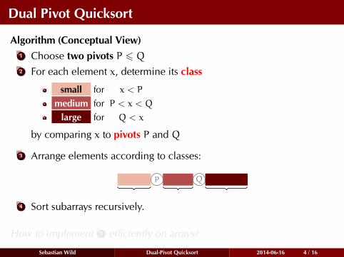
Algorithm (Conceptual View)1 Choose two pivots P 6 Q2 For each element x, determine its class
small for x < P
medium for P < x < Q
large for Q < x
by comparing x to pivots P and Q
3 Arrange elements according to classes:
P Q
4 Sort subarrays recursively.
How to implement 3 efficiently on arrays?
Sebastian Wild Dual-Pivot Quicksort 2014-06-16 4 / 16

Dual Pivot Quicksort
Algorithm (Conceptual View)1 Choose two pivots P 6 Q2 For each element x, determine its class
small for x < P
medium for P < x < Q
large for Q < x
by comparing x to pivots P and Q
3 Arrange elements according to classes:
P Q
4 Sort subarrays recursively.
How to implement 3 efficiently on arrays?
Sebastian Wild Dual-Pivot Quicksort 2014-06-16 4 / 16

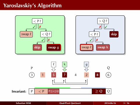
Yaroslavskiy’s Algorithm
< P ?
swap ` < Q ?
skip swap g
3 7
3 7
> Q ?
< P ? skip
swap ` swap k
37
3 7
P Q
3 5 1 7 4 2 8 6
gk̀
P QInvariant:
Sebastian Wild Dual-Pivot Quicksort 2014-06-16 5 / 16

Yaroslavskiy’s Algorithm
< P ?
swap ` < Q ?
skip swap g
3 7
3 7
> Q ?
< P ? skip
swap ` swap k
37
3 7
P Q
3 5 1 7 4 2 8 6
gk̀
P QInvariant:
Sebastian Wild Dual-Pivot Quicksort 2014-06-16 5 / 16

Yaroslavskiy’s Algorithm
< P ?
swap ` < Q ?
skip swap g
3 7
3 7
> Q ?
< P ? skip
swap ` swap k
37
3 7
P Q
3 5 1 7 4 2 8 6
gk̀
P QInvariant:
Sebastian Wild Dual-Pivot Quicksort 2014-06-16 5 / 16

Yaroslavskiy’s Algorithm
< P ?
swap ` < Q ?
skip swap g
3 7
3 7
> Q ?
< P ? skip
swap ` swap k
37
3 7
P Q
3 5 1 7 4 2 8 6
gk̀
P QInvariant:
Sebastian Wild Dual-Pivot Quicksort 2014-06-16 5 / 16

Yaroslavskiy’s Algorithm
< P ?
swap ` < Q ?
skip swap g
3 7
3 7
> Q ?
< P ? skip
swap ` swap k
37
3 7
P Q
3 5 1 7 4 2 8 6
g` k
P≤◦≤QP QInvariant:
Sebastian Wild Dual-Pivot Quicksort 2014-06-16 5 / 16

Yaroslavskiy’s Algorithm
< P ?
swap ` < Q ?
skip swap g
3 7
3 7
> Q ?
< P ? skip
swap ` swap k
37
3 7
P Q
3 5 1 7 4 2 8 6
g` k
P≤◦≤QP QInvariant:
Sebastian Wild Dual-Pivot Quicksort 2014-06-16 5 / 16

Yaroslavskiy’s Algorithm
< P ?
swap ` < Q ?
skip swap g
3 7
3 7
> Q ?
< P ? skip
swap ` swap k
37
3 7
P Q
3 1 5 7 4 2 8 6
g` k
P≤◦≤QP QInvariant:
Sebastian Wild Dual-Pivot Quicksort 2014-06-16 5 / 16

Yaroslavskiy’s Algorithm
< P ?
swap ` < Q ?
skip swap g
3 7
3 7
> Q ?
< P ? skip
swap ` swap k
37
3 7
P Q
3 1 5 7 4 2 8 6
g` k
< P P≤◦≤QP QInvariant:
Sebastian Wild Dual-Pivot Quicksort 2014-06-16 5 / 16

Yaroslavskiy’s Algorithm
< P ?
swap ` < Q ?
skip swap g
3 7
3 7
> Q ?
< P ? skip
swap ` swap k
37
3 7
P Q
3 1 5 7 4 2 8 6
g` k
< P P≤◦≤QP QInvariant:
Sebastian Wild Dual-Pivot Quicksort 2014-06-16 5 / 16

Yaroslavskiy’s Algorithm
< P ?
swap ` < Q ?
skip swap g
3 7
3 7
> Q ?
< P ? skip
swap ` swap k
37
3 7
P Q
3 1 5 7 4 2 8 6
g` k
< P P≤◦≤QP QInvariant:
Sebastian Wild Dual-Pivot Quicksort 2014-06-16 5 / 16

Yaroslavskiy’s Algorithm
< P ?
swap ` < Q ?
skip swap g
3 7
3 7
> Q ?
< P ? skip
swap ` swap k
37
3 7
P Q
3 1 5 7 4 2 8 6
g` k
< P P≤◦≤QP QInvariant:
Sebastian Wild Dual-Pivot Quicksort 2014-06-16 5 / 16

Yaroslavskiy’s Algorithm
< P ?
swap ` < Q ?
skip swap g
3 7
3 7
> Q ?
< P ? skip
swap ` swap k
37
3 7
P Q
3 1 5 7 4 2 8 6
g` k
< P P≤◦≤QP QInvariant:
Sebastian Wild Dual-Pivot Quicksort 2014-06-16 5 / 16

Yaroslavskiy’s Algorithm
< P ?
swap ` < Q ?
skip swap g
3 7
3 7
> Q ?
< P ? skip
swap ` swap k
37
3 7
P Q
3 1 5 7 4 2 8 6
g` k
< P P≤◦≤Q ≥ QP QInvariant:
Sebastian Wild Dual-Pivot Quicksort 2014-06-16 5 / 16

Yaroslavskiy’s Algorithm
< P ?
swap ` < Q ?
skip swap g
3 7
3 7
> Q ?
< P ? skip
swap ` swap k
37
3 7
P Q
3 1 5 7 4 2 8 6
g` k
< P P≤◦≤Q ≥ QP QInvariant:
Sebastian Wild Dual-Pivot Quicksort 2014-06-16 5 / 16
Yaroslavskiy’s Algorithm
< P ?
swap ` < Q ?
skip swap g
3 7
3 7
> Q ?
< P ? skip
swap ` swap k
37
3 7
P Q
3 1 5 7 4 2 8 6
g` k
< P P≤◦≤Q ≥ QP QInvariant:
Sebastian Wild Dual-Pivot Quicksort 2014-06-16 5 / 16

Yaroslavskiy’s Algorithm
< P ?
swap ` < Q ?
skip swap g
3 7
3 7
> Q ?
< P ? skip
swap ` swap k
37
3 7
P Q
3 1 2 5 4 7 8 6
g` k
< P P≤◦≤Q ≥ QP QInvariant:
Sebastian Wild Dual-Pivot Quicksort 2014-06-16 5 / 16

Yaroslavskiy’s Algorithm
< P ?
swap ` < Q ?
skip swap g
3 7
3 7
> Q ?
< P ? skip
swap ` swap k
37
3 7
P Q
3 1 2 5 4 7 8 6
g` k
< P P≤◦≤Q ≥ QP QInvariant:
Sebastian Wild Dual-Pivot Quicksort 2014-06-16 5 / 16

Yaroslavskiy’s Algorithm
< P ?
swap ` < Q ?
skip swap g
3 7
3 7
> Q ?
< P ? skip
swap ` swap k
37
3 7
P Q
3 1 2 5 4 7 8 6
g` k
< P P≤◦≤Q ≥ QP QInvariant:
Sebastian Wild Dual-Pivot Quicksort 2014-06-16 5 / 16

Yaroslavskiy’s Algorithm
< P ?
swap ` < Q ?
skip swap g
3 7
3 7
> Q ?
< P ? skip
swap ` swap k
37
3 7
P Q
3 1 2 5 4 7 8 6
g` k
< P P≤◦≤Q ≥ QP QInvariant:
Sebastian Wild Dual-Pivot Quicksort 2014-06-16 5 / 16

Yaroslavskiy’s Algorithm
< P ?
swap ` < Q ?
skip swap g
3 7
3 7
> Q ?
< P ? skip
swap ` swap k
37
3 7
P Q
3 1 2 5 4 7 8 6
Sebastian Wild Dual-Pivot Quicksort 2014-06-16 5 / 16

Yaroslavskiy’s Algorithm
< P ?
swap ` < Q ?
skip swap g
3 7
3 7
> Q ?
< P ? skip
swap ` swap k
37
3 7
P Q
2 1 3 5 4 6 8 7
Sebastian Wild Dual-Pivot Quicksort 2014-06-16 5 / 16

Yaroslavskiy’s Algorithm
< P ?
swap ` < Q ?
skip swap g
3 7
3 7
> Q ?
< P ? skip
swap ` swap k
37
3 7
P Q
1 2 3 4 5 6 7 8
Sebastian Wild Dual-Pivot Quicksort 2014-06-16 5 / 16

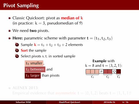
Pivot Sampling
Classic Quicksort: pivot as median of k(in practice: k = 3, pseudomedian of 9)
We need two pivots.
Here: parametric scheme with parameter t = (t1, t2, t3)
1 Sample k = t1 + t2 + t3 + 2 elements2 Sort the sample3 Select pivots s. t. in sorted sample
t1 smaller ,
t2 between and
t3 larger than pivots
Example withk = 8 and t = (3, 2, 1):
P Q
t1 t2 t3
ALENEX 2013:Empirical evidence that asymmetric t = (0, 1, 2) beats t = (1, 1, 1)!
Sebastian Wild Dual-Pivot Quicksort 2014-06-16 6 / 16

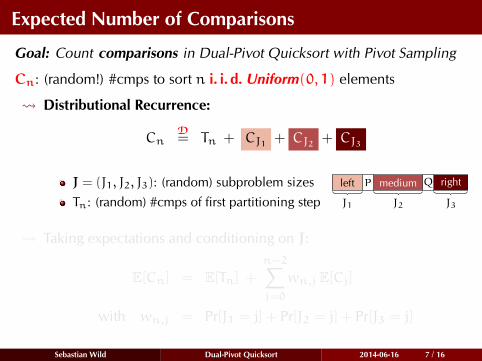
Expected Number of Comparisons
Goal: Count comparisons in Dual-Pivot Quicksort with Pivot Sampling
Cn: (random!) #cmps to sort n i. i. d. Uniform(0, 1) elements
Distributional Recurrence:
CnD= Tn + CJ1 + CJ2 + CJ3
J = (J1, J2, J3): (random) subproblem sizes left medium rightP Q
J1 J2 J3Tn: (random) #cmps of first partitioning step
Taking expectations and conditioning on J:
E[Cn] = E[Tn] +n−2∑j=0
wn,j E[Cj]
with wn,j = Pr[J1 = j] + Pr[J2 = j] + Pr[J3 = j]
Sebastian Wild Dual-Pivot Quicksort 2014-06-16 7 / 16

Solution of Recurrence
Recurrence: E[Cn] = E[Tn] +n−2∑j=0
wn,j E[Cj] with E[Tn] ∼ γn
Apply Continuous Master Theorem [Roura 2001]Idea: Approximate sum by integral over relative subprobem size α = j/n
n−2∑j=0
wn,j E[Cj] ≈ˆ n0
wn,j E[Cj]dj ≈ˆ 10
n ·wn,αn E[Cαn]dα
Continuous Recurrence: E[Cn] ≈ E[Tn] +ˆ 10
w(α)E[Cαn]dα
Ansatz: E[Cn] = γHn lnn
fulfills recurrence for H =
3∑l=1
tl + 1
k+ 1
(Hk+1 −Htl+1
) E[Cn] ∼
γ
Hn lnn Next: What is γ?
Sebastian Wild Dual-Pivot Quicksort 2014-06-16 8 / 16

Solution of Recurrence
Recurrence: E[Cn] = E[Tn] +n−2∑j=0
wn,j E[Cj] with E[Tn] ∼ γn
Apply Continuous Master Theorem [Roura 2001]Idea: Approximate sum by integral over relative subprobem size α = j/n
n−2∑j=0
wn,j E[Cj] ≈ˆ n0
wn,j E[Cj]dj ≈ˆ 10
n ·wn,αn︸ ︷︷ ︸→ w(α)
E[Cαn]dα
Continuous Recurrence: E[Cn] ≈ E[Tn] +ˆ 10
w(α)E[Cαn]dα
Ansatz: E[Cn] = γHn lnn
fulfills recurrence for H =
3∑l=1
tl + 1
k+ 1
(Hk+1 −Htl+1
) E[Cn] ∼
γ
Hn lnn Next: What is γ?
Sebastian Wild Dual-Pivot Quicksort 2014-06-16 8 / 16

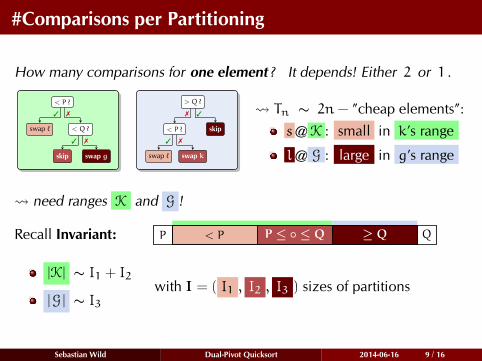
#Comparisons per Partitioning
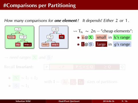
How many comparisons for one element? It depends! Either 2 or 1 .
< P ?
swap ` < Q ?
skip swap g
3 7
3 7
> Q ?
< P ? skip
swap ` swap k
37
3 7
Tn ∼ 2n− ”cheap elements”:
s@K : small in k’s range
l@ G : large in g’s range
need ranges K and G !
Recall Invariant: < P P ≤ ◦ ≤ Q ≥ QP Q
|K| ∼ I1 + I2
|G | ∼ I3with I = ( I1 , I2 , I3 ) sizes of partitions
Sebastian Wild Dual-Pivot Quicksort 2014-06-16 9 / 16

#Comparisons per Partitioning
How many comparisons for one element? It depends! Either 2 or 1 .
< P ?
swap ` < Q ?
skip swap g
3 7
3 7
> Q ?
< P ? skip
swap ` swap k
37
3 7
Tn ∼ 2n− ”cheap elements”:
s@K : small in k’s range
l@ G : large in g’s range
need ranges K and G !
Recall Invariant: < P P ≤ ◦ ≤ Q ≥ QP Q
|K| ∼ I1 + I2
|G | ∼ I3with I = ( I1 , I2 , I3 ) sizes of partitions
Sebastian Wild Dual-Pivot Quicksort 2014-06-16 9 / 16

Distribution of s@K and l@G
Consider I fixed.|K| ∼ I1 + I2|G | ∼ I3
#small = I1
#large = I3
s@KD= Hypergeometric( #small , |K| , n− k)
[sample excludedfrom partitioning n− k
]
Draw positions of small elements:1 All array indices in urn2 Draw without replacement3 Count green balls
1
34
67
28
5
2 8 5
I = (3, 2, 3)
1 2 3 4 5 6 7 8
s@K = 2
Similarly: l@ GD= Hypergeometric( #large , |G| , n− k)
Sebastian Wild Dual-Pivot Quicksort 2014-06-16 10 / 16

Distribution of s@K and l@G
Consider I fixed.|K| ∼ I1 + I2|G | ∼ I3
#small = I1
#large = I3
s@KD= Hypergeometric( #small , |K| , n− k)
[sample excludedfrom partitioning n− k
]
Draw positions of small elements:1 All array indices in urn2 Draw without replacement3 Count green balls
1
34
67
85
2
8 5
I = (3, 2, 3)
1 2 3 4 5 6 7 8
s@K = 2
Similarly: l@ GD= Hypergeometric( #large , |G| , n− k)
Sebastian Wild Dual-Pivot Quicksort 2014-06-16 10 / 16

Distribution of s@K and l@G
Consider I fixed.|K| ∼ I1 + I2|G | ∼ I3
#small = I1
#large = I3
s@KD= Hypergeometric( #small , |K| , n− k)
[sample excludedfrom partitioning n− k
]
Draw positions of small elements:1 All array indices in urn2 Draw without replacement3 Count green balls
1
34
67
5
2 8
5
I = (3, 2, 3)
1 2 3 4 5 6 7 8
s@K = 2
Similarly: l@ GD= Hypergeometric( #large , |G| , n− k)
Sebastian Wild Dual-Pivot Quicksort 2014-06-16 10 / 16

Distribution of s@K and l@G
Consider I fixed.|K| ∼ I1 + I2|G | ∼ I3
#small = I1
#large = I3
s@KD= Hypergeometric( #small , |K| , n− k)
[sample excludedfrom partitioning n− k
]
Draw positions of small elements:1 All array indices in urn2 Draw without replacement3 Count green balls
1
34
67
2 8 5
I = (3, 2, 3)
1 2 3 4 5 6 7 8
s@K = 2
Similarly: l@ GD= Hypergeometric( #large , |G| , n− k)
Sebastian Wild Dual-Pivot Quicksort 2014-06-16 10 / 16

Distribution of s@K and l@G
Consider I fixed.|K| ∼ I1 + I2|G | ∼ I3
#small = I1
#large = I3
s@KD= Hypergeometric( #small , |K| , n− k)
[sample excludedfrom partitioning n− k
]
Draw positions of small elements:1 All array indices in urn2 Draw without replacement3 Count green balls
1
34
67
2 8 5
I = (3, 2, 3)
1 2 3 4 5 6 7 8
s@K = 2
Similarly: l@ GD= Hypergeometric( #large , |G| , n− k)
Sebastian Wild Dual-Pivot Quicksort 2014-06-16 10 / 16

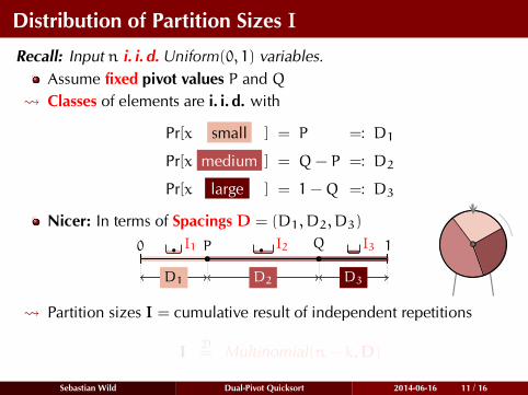
Distribution of Partition Sizes I
Recall: Input n i. i. d. Uniform(0, 1) variables.Assume fixed pivot values P and Q
Classes of elements are i. i. d. with
Pr[x small ] = P
=: D1
Pr[x medium ] = Q− P
=: D2
Pr[x large ] = 1−Q
=: D3
Nicer: In terms of Spacings D = (D1, D2, D3)
0 1P Q
Partition sizes I = cumulative result of independent repetitions
ID= Multinomial(n− k,D)
Sebastian Wild Dual-Pivot Quicksort 2014-06-16 11 / 16

Distribution of Partition Sizes I
Recall: Input n i. i. d. Uniform(0, 1) variables.Assume fixed pivot values P and Q
Classes of elements are i. i. d. with
Pr[x small ] = P =: D1
Pr[x medium ] = Q− P =: D2
Pr[x large ] = 1−Q =: D3
Nicer: In terms of Spacings D = (D1, D2, D3)
0 1P Q
D1 D2 D3
I1 I2 I3
Partition sizes I = cumulative result of independent repetitions
ID= Multinomial(n− k,D)
Sebastian Wild Dual-Pivot Quicksort 2014-06-16 11 / 16

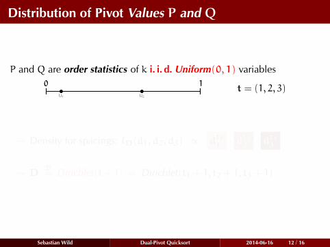
Distribution of Pivot Values P and Q
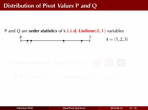
P and Q are order statistics of k i. i. d. Uniform(0, 1) variables0 10 1
t = (1, 2, 3)
Density for spacings: fD(d1, d2, d3) ∝ dt11 · dt22 · d
t33
DD= Dirichlet(t+ 1) = Dirichlet(t1 + 1, t2 + 1, t3 + 1)
Sebastian Wild Dual-Pivot Quicksort 2014-06-16 12 / 16

Distribution of Pivot Values P and Q
P and Q are order statistics of k i. i. d. Uniform(0, 1) variables0 1
U1
0 1t = (1, 2, 3)
Density for spacings: fD(d1, d2, d3) ∝ dt11 · dt22 · d
t33
DD= Dirichlet(t+ 1) = Dirichlet(t1 + 1, t2 + 1, t3 + 1)
Sebastian Wild Dual-Pivot Quicksort 2014-06-16 12 / 16
Distribution of Pivot Values P and Q
P and Q are order statistics of k i. i. d. Uniform(0, 1) variables0 1
U1 U2
0 1t = (1, 2, 3)
Density for spacings: fD(d1, d2, d3) ∝ dt11 · dt22 · d
t33
DD= Dirichlet(t+ 1) = Dirichlet(t1 + 1, t2 + 1, t3 + 1)
Sebastian Wild Dual-Pivot Quicksort 2014-06-16 12 / 16

Distribution of Pivot Values P and Q
P and Q are order statistics of k i. i. d. Uniform(0, 1) variables0 1
U1 U2U3
0 1t = (1, 2, 3)
Density for spacings: fD(d1, d2, d3) ∝ dt11 · dt22 · d
t33
DD= Dirichlet(t+ 1) = Dirichlet(t1 + 1, t2 + 1, t3 + 1)
Sebastian Wild Dual-Pivot Quicksort 2014-06-16 12 / 16
Distribution of Pivot Values P and Q
P and Q are order statistics of k i. i. d. Uniform(0, 1) variables0 1
U1 U2U3 U4
0 1t = (1, 2, 3)
Density for spacings: fD(d1, d2, d3) ∝ dt11 · dt22 · d
t33
DD= Dirichlet(t+ 1) = Dirichlet(t1 + 1, t2 + 1, t3 + 1)
Sebastian Wild Dual-Pivot Quicksort 2014-06-16 12 / 16

Distribution of Pivot Values P and Q
P and Q are order statistics of k i. i. d. Uniform(0, 1) variables0 1
U1 U2U3 U4U5
0 1t = (1, 2, 3)
Density for spacings: fD(d1, d2, d3) ∝ dt11 · dt22 · d
t33
DD= Dirichlet(t+ 1) = Dirichlet(t1 + 1, t2 + 1, t3 + 1)
Sebastian Wild Dual-Pivot Quicksort 2014-06-16 12 / 16

Distribution of Pivot Values P and Q
P and Q are order statistics of k i. i. d. Uniform(0, 1) variables0 1
U1 U2U3 U4U5 U6
0 1t = (1, 2, 3)
Density for spacings: fD(d1, d2, d3) ∝ dt11 · dt22 · d
t33
DD= Dirichlet(t+ 1) = Dirichlet(t1 + 1, t2 + 1, t3 + 1)
Sebastian Wild Dual-Pivot Quicksort 2014-06-16 12 / 16

Distribution of Pivot Values P and Q
P and Q are order statistics of k i. i. d. Uniform(0, 1) variables0 1
U1 U2U3 U4U5 U6 U7
0 1t = (1, 2, 3)
Density for spacings: fD(d1, d2, d3) ∝ dt11 · dt22 · d
t33
DD= Dirichlet(t+ 1) = Dirichlet(t1 + 1, t2 + 1, t3 + 1)
Sebastian Wild Dual-Pivot Quicksort 2014-06-16 12 / 16

Distribution of Pivot Values P and Q
P and Q are order statistics of k i. i. d. Uniform(0, 1) variables0 1
U1 U2U3 U4U5 U6 U7U8
P Q0 1
D1 D2 D3
t = (1, 2, 3)
Density for spacings: fD(d1, d2, d3) ∝ dt11 · dt22 · d
t33
DD= Dirichlet(t+ 1) = Dirichlet(t1 + 1, t2 + 1, t3 + 1)
Sebastian Wild Dual-Pivot Quicksort 2014-06-16 12 / 16

Distribution of Pivot Values P and Q
P and Q are order statistics of k i. i. d. Uniform(0, 1) variables0 1
U1 U2U3 U4U5 U6 U7U8
P Q0 1
D1 D2 D3
t = (1, 2, 3)
Density for spacings: fD(d1, d2, d3) ∝ dt11 · dt22 · d
t33
DD= Dirichlet(t+ 1) = Dirichlet(t1 + 1, t2 + 1, t3 + 1)
Sebastian Wild Dual-Pivot Quicksort 2014-06-16 12 / 16

Expected #Comparisons per Partitioning
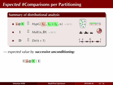
Summary of distributional analysis
s@ KD= HypG( I1 , I1 + I2 , n) +O(1)
1
34
67
28
51 2 3 4 5 6 7 8
ID= Mult(n,D) +O(1)
DD= Dir(t+ 1) 0 1P Q
expected value by successive unconditioning:
ED[EI[E[ s@K | I]
∣∣ D]] =(t1 + 1)(t1 + t2 + 3)
(k+ 2)(k+ 1)· n +O(1)
ED[EI[E[ l@ G | I]
∣∣ D]] =(t3 + 2)(t3 + 1)
(k+ 2)(k+ 1)· n +O(1)
Sebastian Wild Dual-Pivot Quicksort 2014-06-16 13 / 16

Expected #Comparisons per Partitioning
Summary of distributional analysis
s@ KD= HypG( I1 , I1 + I2 , n) +O(1)
1
34
67
28
51 2 3 4 5 6 7 8
ID= Mult(n,D) +O(1)
DD= Dir(t+ 1) 0 1P Q
expected value by successive unconditioning:
ED[EI[
E[ s@K
| I
]
∣∣ D]] =(t1 + 1)(t1 + t2 + 3)
(k+ 2)(k+ 1)· n +O(1)
ED[EI[E[ l@ G | I]
∣∣ D]] =(t3 + 2)(t3 + 1)
(k+ 2)(k+ 1)· n +O(1)
Sebastian Wild Dual-Pivot Quicksort 2014-06-16 13 / 16
Expected #Comparisons per Partitioning
Summary of distributional analysis
s@ KD= HypG( I1 , I1 + I2 , n) +O(1)
1
34
67
28
51 2 3 4 5 6 7 8
ID= Mult(n,D) +O(1)
DD= Dir(t+ 1) 0 1P Q
expected value by successive unconditioning:
ED[EI[
E[ s@K | I]
∣∣ D]] =(t1 + 1)(t1 + t2 + 3)
(k+ 2)(k+ 1)· n +O(1)
ED[EI[E[ l@ G | I]
∣∣ D]] =(t3 + 2)(t3 + 1)
(k+ 2)(k+ 1)· n +O(1)
Sebastian Wild Dual-Pivot Quicksort 2014-06-16 13 / 16

Expected #Comparisons per Partitioning
Summary of distributional analysis
s@ KD= HypG( I1 , I1 + I2 , n) +O(1)
1
34
67
28
51 2 3 4 5 6 7 8
ID= Mult(n,D) +O(1)
DD= Dir(t+ 1) 0 1P Q
expected value by successive unconditioning:
ED[
EI[E[ s@K | I]
∣∣ D]
]=
(t1 + 1)(t1 + t2 + 3)
(k+ 2)(k+ 1)· n +O(1)
ED[EI[E[ l@ G | I]
∣∣ D]] =(t3 + 2)(t3 + 1)
(k+ 2)(k+ 1)· n +O(1)
Sebastian Wild Dual-Pivot Quicksort 2014-06-16 13 / 16

Expected #Comparisons per Partitioning
Summary of distributional analysis
s@ KD= HypG( I1 , I1 + I2 , n) +O(1)
1
34
67
28
51 2 3 4 5 6 7 8
ID= Mult(n,D) +O(1)
DD= Dir(t+ 1) 0 1P Q
expected value by successive unconditioning:
ED[EI[E[ s@K | I]
∣∣ D]]
=(t1 + 1)(t1 + t2 + 3)
(k+ 2)(k+ 1)· n +O(1)
ED[EI[E[ l@ G | I]
∣∣ D]] =(t3 + 2)(t3 + 1)
(k+ 2)(k+ 1)· n +O(1)
Sebastian Wild Dual-Pivot Quicksort 2014-06-16 13 / 16

Expected #Comparisons per Partitioning
Summary of distributional analysis
s@ KD= HypG( I1 , I1 + I2 , n) +O(1)
1
34
67
28
51 2 3 4 5 6 7 8
ID= Mult(n,D) +O(1)
DD= Dir(t+ 1) 0 1P Q
expected value by successive unconditioning:
ED[EI[E[ s@K | I]
∣∣ D]] =(t1 + 1)(t1 + t2 + 3)
(k+ 2)(k+ 1)· n +O(1)
ED[EI[E[ l@ G | I]
∣∣ D]] =(t3 + 2)(t3 + 1)
(k+ 2)(k+ 1)· n +O(1)
Sebastian Wild Dual-Pivot Quicksort 2014-06-16 13 / 16

Expected #Comparisons per Partitioning
Summary of distributional analysis
s@ KD= HypG( I1 , I1 + I2 , n) +O(1)
1
34
67
28
51 2 3 4 5 6 7 8
ID= Mult(n,D) +O(1)
DD= Dir(t+ 1) 0 1P Q
expected value by successive unconditioning:
ED[EI[E[ s@K | I]
∣∣ D]] =(t1 + 1)(t1 + t2 + 3)
(k+ 2)(k+ 1)· n +O(1)
ED[EI[E[ l@ G | I]
∣∣ D]] =(t3 + 2)(t3 + 1)
(k+ 2)(k+ 1)· n +O(1)
Sebastian Wild Dual-Pivot Quicksort 2014-06-16 13 / 16

Expected #Comparisons
Final Result: E[Cn] ∼γ
H· n lnn
Sebastian Wild Dual-Pivot Quicksort 2014-06-16 14 / 16

Expected #Comparisons
Final Result: E[Cn] ∼γ
3∑l=1
tl + 1
k+ 1
(Hk+1 −Htl+1
) · n lnn
Sebastian Wild Dual-Pivot Quicksort 2014-06-16 14 / 16

Expected #Comparisons
Final Result: E[Cn] ∼2 −
s@K
n−
l@G
n
3∑l=1
tl + 1
k+ 1
(Hk+1 −Htl+1
) · n lnn
Sebastian Wild Dual-Pivot Quicksort 2014-06-16 14 / 16

Expected #Comparisons
Final Result: E[Cn] ∼2 −
(t1 + 1)(t1 + t2 + 3)
(k+ 2)(k+ 1)−
(t3 + 2)(t3 + 1)
(k+ 2)(k+ 1)
3∑l=1
tl + 1
k+ 1
(Hk+1 −Htl+1
) · n lnn
Sebastian Wild Dual-Pivot Quicksort 2014-06-16 14 / 16

Expected #Comparisons
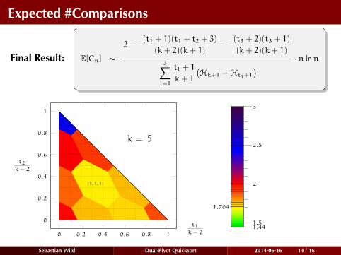
Final Result: E[Cn] ∼2 −
(t1 + 1)(t1 + t2 + 3)
(k+ 2)(k+ 1)−
(t3 + 2)(t3 + 1)
(k+ 2)(k+ 1)
3∑l=1
tl + 1
k+ 1
(Hk+1 −Htl+1
) · n lnn
. . . a little hard to interpret.
Let’s have some pictures.
Sebastian Wild Dual-Pivot Quicksort 2014-06-16 14 / 16

Expected #Comparisons
Final Result: E[Cn] ∼2 −
(t1 + 1)(t1 + t2 + 3)
(k+ 2)(k+ 1)−
(t3 + 2)(t3 + 1)
(k+ 2)(k+ 1)
3∑l=1
tl + 1
k+ 1
(Hk+1 −Htl+1
) · n lnn
0 0.2 0.4 0.6 0.8 1
0
0.2
0.4
0.6
0.8
1
k = 2
(0,0, 0)
t1k− 2
t2k− 2
1.44
3
2
2.5
1.5
1.9
Sebastian Wild Dual-Pivot Quicksort 2014-06-16 14 / 16
Expected #Comparisons
Final Result: E[Cn] ∼2 −
(t1 + 1)(t1 + t2 + 3)
(k+ 2)(k+ 1)−
(t3 + 2)(t3 + 1)
(k+ 2)(k+ 1)
3∑l=1
tl + 1
k+ 1
(Hk+1 −Htl+1
) · n lnn
0 0.2 0.4 0.6 0.8 1
0
0.2
0.4
0.6
0.8
1
k = 5
(1,1, 1)
t1k− 2
t2k− 2
1.44
3
2
2.5
1.5
1.704
Sebastian Wild Dual-Pivot Quicksort 2014-06-16 14 / 16
Expected #Comparisons
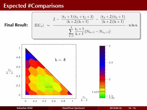
Final Result: E[Cn] ∼2 −
(t1 + 1)(t1 + t2 + 3)
(k+ 2)(k+ 1)−
(t3 + 2)(t3 + 1)
(k+ 2)(k+ 1)
3∑l=1
tl + 1
k+ 1
(Hk+1 −Htl+1
) · n lnn
0 0.2 0.4 0.6 0.8 1
0
0.2
0.4
0.6
0.8
1
k = 8
(3,1, 2)
t1k− 2
t2k− 2
1.44
3
2
2.5
1.5
1.623
Sebastian Wild Dual-Pivot Quicksort 2014-06-16 14 / 16

Expected #Comparisons
Final Result: E[Cn] ∼2 −
(t1 + 1)(t1 + t2 + 3)
(k+ 2)(k+ 1)−
(t3 + 2)(t3 + 1)
(k+ 2)(k+ 1)
3∑l=1
tl + 1
k+ 1
(Hk+1 −Htl+1
) · n lnn
0 0.2 0.4 0.6 0.8 1
0
0.2
0.4
0.6
0.8
1
k = 11
(4,2, 3)
t1k− 2
t2k− 2
1.44
3
2
2.5
1.51.585
Sebastian Wild Dual-Pivot Quicksort 2014-06-16 14 / 16

Expected #Comparisons
Final Result: E[Cn] ∼2 −
(t1 + 1)(t1 + t2 + 3)
(k+ 2)(k+ 1)−
(t3 + 2)(t3 + 1)
(k+ 2)(k+ 1)
3∑l=1
tl + 1
k+ 1
(Hk+1 −Htl+1
) · n lnn
0 0.2 0.4 0.6 0.8 1
0
0.2
0.4
0.6
0.8
1
k = ∞
t1k− 2
t2k− 2
1.44
3
2
2.5
1.51.4931
Sebastian Wild Dual-Pivot Quicksort 2014-06-16 14 / 16

Expected #Comparisons
Final Result: E[Cn] ∼2 −
(t1 + 1)(t1 + t2 + 3)
(k+ 2)(k+ 1)−
(t3 + 2)(t3 + 1)
(k+ 2)(k+ 1)
3∑l=1
tl + 1
k+ 1
(Hk+1 −Htl+1
) · n lnn
0 0.2 0.4 0.6 0.8 1
0
0.2
0.4
0.6
0.8
1
k = ∞
(0.429,0.269,0.302)
t1k− 2
t2k− 2
1.44
3
2
2.5
1.51.49311.5171
Sebastian Wild Dual-Pivot Quicksort 2014-06-16 14 / 16

Beyond Comparisons
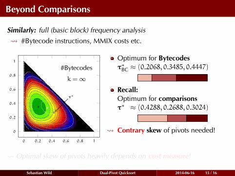
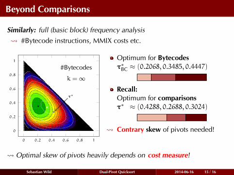
Similarly: full (basic block) frequency analysis
#Bytecode instructions, MMIX costs etc.
0 0.2 0.4 0.6 0.8 1
0
0.2
0.4
0.6
0.8
1
#Bytecodes
Optimum for Bytecodesτ∗BC ≈ (0.2068, 0.3485, 0.4447)
Recall:Optimum for comparisonsτ∗ ≈ (0.4288, 0.2688, 0.3024)
Contrary skew of pivots needed!
Optimal skew of pivots heavily depends on cost measure!
Sebastian Wild Dual-Pivot Quicksort 2014-06-16 15 / 16

Beyond Comparisons
Similarly: full (basic block) frequency analysis
#Bytecode instructions, MMIX costs etc.
0 0.2 0.4 0.6 0.8 1
0
0.2
0.4
0.6
0.8
1
k = 5
(0,1, 2)
k = 8
#Bytecodes
Optimum for Bytecodesτ∗BC ≈ (0.2068, 0.3485, 0.4447)
Recall:Optimum for comparisonsτ∗ ≈ (0.4288, 0.2688, 0.3024)
Contrary skew of pivots needed!
Optimal skew of pivots heavily depends on cost measure!
Sebastian Wild Dual-Pivot Quicksort 2014-06-16 15 / 16

Beyond Comparisons
Similarly: full (basic block) frequency analysis
#Bytecode instructions, MMIX costs etc.
0 0.2 0.4 0.6 0.8 1
0
0.2
0.4
0.6
0.8
1
k = 5
(0,1, 2)
k = 8k = 11
#Bytecodes
Optimum for Bytecodesτ∗BC ≈ (0.2068, 0.3485, 0.4447)
Recall:Optimum for comparisonsτ∗ ≈ (0.4288, 0.2688, 0.3024)
Contrary skew of pivots needed!
Optimal skew of pivots heavily depends on cost measure!
Sebastian Wild Dual-Pivot Quicksort 2014-06-16 15 / 16

Beyond Comparisons
Similarly: full (basic block) frequency analysis
#Bytecode instructions, MMIX costs etc.
0 0.2 0.4 0.6 0.8 1
0
0.2
0.4
0.6
0.8
1
k = 5
(0,1, 2)
k = 8k = 11k = ∞#Bytecodes
Optimum for Bytecodesτ∗BC ≈ (0.2068, 0.3485, 0.4447)
Recall:Optimum for comparisonsτ∗ ≈ (0.4288, 0.2688, 0.3024)
Contrary skew of pivots needed!
Optimal skew of pivots heavily depends on cost measure!
Sebastian Wild Dual-Pivot Quicksort 2014-06-16 15 / 16

Beyond Comparisons
Similarly: full (basic block) frequency analysis
#Bytecode instructions, MMIX costs etc.
0 0.2 0.4 0.6 0.8 1
0
0.2
0.4
0.6
0.8
1
k = 5
(0,1, 2)
k = 8k = 11k = ∞k = ∞#Bytecodes
τ∗
Optimum for Bytecodesτ∗BC ≈ (0.2068, 0.3485, 0.4447)
Recall:Optimum for comparisonsτ∗ ≈ (0.4288, 0.2688, 0.3024)
Contrary skew of pivots needed!
Optimal skew of pivots heavily depends on cost measure!
Sebastian Wild Dual-Pivot Quicksort 2014-06-16 15 / 16
Conclusion
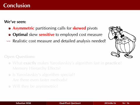
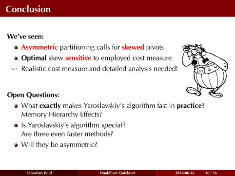
We’ve seen:Asymmetric partitioning calls for skewed pivots
Optimal skew sensitive to employed cost measure
Realistic cost measure and detailed analysis needed!
Open Questions:What exactly makes Yaroslavskiy’s algorithm fast in practice?Memory Hierarchy Effects?
Is Yaroslavskiy’s algorithm special ?Are there even faster methods?
Will they be asymmetric?
Sebastian Wild Dual-Pivot Quicksort 2014-06-16 16 / 16
Conclusion
We’ve seen:Asymmetric partitioning calls for skewed pivots
Optimal skew sensitive to employed cost measure
Realistic cost measure and detailed analysis needed!
Open Questions:What exactly makes Yaroslavskiy’s algorithm fast in practice?Memory Hierarchy Effects?
Is Yaroslavskiy’s algorithm special ?Are there even faster methods?
Will they be asymmetric?
Sebastian Wild Dual-Pivot Quicksort 2014-06-16 16 / 16