PISCO

PISCO

H. E. Schwarz

ESO OPERATING MANUAL No. 13

Version No. 1

March 1989

Contents

1 Introduction

2 System description

2.1 Optical layout .

2.2 Diaphragms, acquisition and guiding

2.3 Phase plates and polarizer .

2.4 Filters . . . . . .

2.5 Photomultipliers

2.6 Polaroids

2.7 Modes ..

2.8 Calibrations.

2.8.1 Rotating wave plate time intervals

2.8.2 Angles, self polarization, and efficiency .

2.9 Data format . . . . . . . . . . . . . . . . . . . .

3 Observing

3.1 Starting up and closing down .

3.2 Instrument control and data acquisition

3.3 Measurements ..

3.4 Integration times

3.5 Linear polarization

3.6 Determination of linear polarization

3.7 Determination of circular polarization

3.8 Data reduction . . . . . . . . . . . . .

1

2

2

3

5

5

6

6

6

7

7

8

8

10

10

11

11

11

12

13

14

16

3.9 Trouble shooting . . . . . . . . . . . . . . . . . . . . . . . . . . . . . . . .. 16

Bibliography 16

A Polarimetry 17

A.1 The Stokes parameters . . . . . . . . . . . . . . . . . . . .'. 17

A.2 Muel1er calculus and PISCO .. . . . . . . ..... 20

B Typed commands 22

ii

List of Tables

2.1 PISCO diaphragms . . . . . . . . . . . . . . ..

2.2 Content of scanlines 5, 6 and 7 in the data files

3

9

3.1 Sensitivity of PISCO in UBVRI filters . . . . . . . . . . . . . . . . . . . .. 12

Hi

List of Figures

2.1 Schematic drawing showing the most important parts of the instrument. 4

2.2 The field of view of the polarimeter (large field) . . . . . . . . . . . . . . 5

iv

Chapter 1

Introduction

PISCO is the ESO Polarimeter with Instrumental and £ky i&mpensation, a two channel,filter polarimeter using photon counting, offered on the ESO IMPI 2.2 m telescope.

The instrument is capable of high precision linear and circular polarimetry of objects downto ~17th magnitude.

This manual is intended to assist users of PISCO with their preparation of observations,observing and to give hints on data reduction. For observers with little or no polarimetryexperience, appendix A gives some background on the techni~ues.

This manual is not intended for use as an in depth technical reference work. For detailedinformation of this kind a separate technical manual is available.

We strongly encourage users to make any comments and suggestions concerning this man­ual in order that we may refine future versions. Please do this by firstly writing on a copyof this manual which you will find in the control room of the telescope and secondly inyour observing report to be completed at the end of your observing mission to La Silla.

1

Chapter 2

System description

2.1 Optical layout

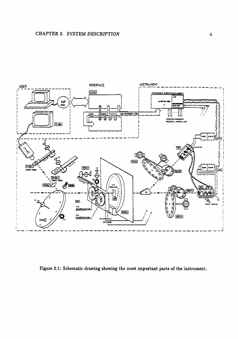
PISCO is a two-channel polarimeter (see e.g. Serkowski, 1974 for polarimeter designs ofthis type). A schematic view of the instrument is shown in Figure 2.1. The light entersthe instrument through the inclined diaphragm wheel DIAPW. Via the mirrored surfaceof this wheel, a TV camera views the observed field. Setting and -guiding is done withthe use of this camera. The compensating phase plate unit CPP corrects for the effects ofthe rotating half-wave plate RPP and automatically compensates for the sky polarizationif a two-hole integration is ·used. The Foster prism FP separates the ordinary and theextraordinary beams. The selection of the wavelength range is done via the colour filterwheels XCFLTW and YCFLTW separately for the X and Y channel. If the same filtersare chosen for both channels, the instrument operates in the two-channel mode. Thedensity filters XDFLTW and YDFLTW are inserted if very bright stars are observed. Thephotons are detected by the multipliers XMP and YMP. A Z80 microprocessor performsthe integration of the counts in 2 x 32 channels. The user controls all functions of theinstrument via the HP 1000 computer and a CAMAC interface.

All lenses, prisms and cover glasses of the retarders are made of fused silica thus guarantee­ing a high transparency between 3000 and 11000 A. However, since the use of achromaticlenses is not possible in most parts of the polarimeter, the useful wavelength range remainsrestricted to the range from 3400 Ato 8500 A. All optical surfaces are provided as far aspossible with antireflection coatings. In contrast to the usual design it does not use a Wol­laston prism but a modified Foster prism to separate the ordinary and the extraordinarybeam. This design has the advantage of a large (45°) and wavelength independent beamseparation.

2

CHAPTER 2. SYSTEM DESCRIPTION 3

The principal new feature of PISCO is the possibility to compensate directly for the skypolarization and partly also for the instrumental polarization. The sky compensationis achieved by using two apertures and two compensating phase plates with differentorientation of the optical axes. The combined sky light is then in principle unpolarized(see Appendix A). The instrumental polarization of the phase plate can be compensatedfor by rotating the whole compensating phase plate unit by 1800 during an integration.This can be done customarily.

The signal modulation is effected by a half-wave plate which rotates at 6 cycles seC l .

Each turn of this half-wave plate is divided into 32 equidistant sectors corresponding to 32counter channels. The sinusoidal modulation of the count rate describes the polarimetricsignal which can be extracted using standard Fourier techniques.

2.2 Diaphragms, acquisition and guiding

PISCO has 8 sets of 2 diaphragms in an inclined, polished diaphragm wheel. The lightreflected from the wheel is viewed by an intensified TV camera for acquisition and guiding.

Each aperture has a corresponding cross hair etched into the wheel. An object should becentered in a cross. When starting an integration the selected aperture will be rotated inplace allowing the light to enter the instrument.

Any suitable star in the field can be used for guiding with the standard ESO auto guider.For bright objects, and when no other stars are in the field, guiding can be done on theaperture itself using the reflected starlight around the edge of the aperture.

The available apertures 1 to 8 are listed in mm and arcseconds in Table 2.1.

Table 2.1: PISCO diaphragms

I aperture number = 4 5 6 7 8diameter [mm] 0.35 0.60 10.85 1.30 1.70 2.15 2.55 3.00diameter ["1 4.00 6.90 19.70 15.0 19.4 24.8 29.4 34.6

The acquisition/guiding TV camera has two sets of lenses mounted in front of it, giving 2fields of view for acquisition and guiding. The large field is about 4' X 6' and the small fieldabout 1:5 X 2' allowing very accurate centering of objects. These fields can be selectedfrom the keyboard. Stars of mv '" 18 or brighter can be used for guiding. Figure 2.2 showsthe acquisition (large) field of PISCO.

CHAPTER 2. SYSTEM DESCRIPTION 4

USER INTERFACE I~~~':"'~ _----------------, I I

! ltF r;' i '''-I ! _..::::::-. ,i (~!<=>L.-_..;;j---i.r---i : \ MlIGPI • II I l----'.....~~~~I---.-. ,', '

I 0 I "I I .1M1. .

i I nl2...' II 14

i I~-I III J I

I

r~'-------u-----------------------

; (~ NI, . ~

I ,~>

I

,I ,

=- ;:,.".. -11

/'

I--- ... _-- ---- --- ------------- ----------- -- ------- ---

Figure 2.1: Schematic drawing showing the most important parts of the instrument.

CHAPTER 2. SYSTEM DESCRIPTION 5

C(

... .. ".. '' .•

•. . .o· •

• ••

•

•

•

. .••

••

•• •

'0 ••®5

.•

. .."

..• •

•

.. ~ "

"305 ':'•. J...·----------r--T'.

Figure 2.2: The field of view of the polarimeter (large field)

2.3 Phase plates and polarizer

After passing through the diaphragm, the light encounters the compensating phase plateswhich invert the appropriate Stokes parameters to eliminate the sky polarization (seeAppendix A). After a field lens the light passes through the rotating halfwave plate whichis the modulator of the signal.

Next is the polarizer which here is a modified Foster prism (Foster, 1938) splitting the lightinto two orthogonally polarized beams which emerge at 45° to each other. Cemented onthe output faces of the Foster prism are depolarizers. These prevent unwanted polarizationeffects in the subsequent optics.

We now have two unpolarized beams which are modulated sinusoidally in intensity de­pending on the amount of linear polarization of the incoming beam. The two channels areindicated by X and Y.

2.4 Filters

The X and Y beams pass through one of the apertures in the colour filter wheels anddensity filter wheels. The colour filter wheels can hold up to 11 different filters while thedensity filter wheel has 3 positions: open, density ND2 and closed (shutter).

CHAPTER 2. SYSTEM DESCRIPTION 6

PISCO has two identical sets of UBVRI filters permanently mounted in positions 1 to 5,positions 0 and 6 are closed and position 7 is open, for white light observations. Positions8 to 11 can be used for any filter 25.4 mm in diameter and up to 10 mm thick. This is thesame for both wheels.

The transmission curves for the UBVRI filters are included in the ESO filter inventoryunder numbers 558 to 567. The U filter has a red leak but CuS04 filters will be installedin the near future.

2.5 Photomultipliers

After passing through the filter wheels, the X and Y beams enter Fabry lenses which forma pupil image on the photocathodes of two Hamamatsu R 943-02 photomultipliers. Theseare GaAs types with properties similar to the Quantacon or RCA 31034A-02 tubes.

The tubes are cooled by refrigerated glycol to give a darkcurrent of'" 20 cts S-1 at 1950 V.The cooler is mounted on the telescope next to the instrument and should be set to -400

•

The display should normally indicate'" -300•

2.6 Polaroids

A polaroid polarizer in a metal holder is available for measurement of wave plate fast axisangles and calibration. The unit can be inserted in the light path before the aperturewheel by removing the diaphragm illuminating lamp unit. This operation is not remotelycontrolled but must be done manually at the instrument.

2.7 Modes

PISCO can be used in several different modes: linear and circular polarization with eithersingle or double apertures (for sky polarization compensation), and with or without arotation of the compensating wave plates half way the integration to correct for some ofthe instrumental effects (mainly the wave plate self polarization).

Below the available modes are briefly described and suggestions given regarding the ap­propriate circumstances in which to use a particular mode.

1. Linear polarization measurement.

(a) One aperture: telescope movement for sky.

(b) Two apertures: one star +sky, the other sky. Telescope movement for skyintensity measurement.

CHAPTER 2. SYSTEM DESCRIPTION 7

Modes la and 1b can be used without (NO) or with (ER) a rotation of the compensat­ing wave plates by 1800 halfway each integration to compensate for the polarizationof the wave plate.

A total of 4 linear modes are therefore available.

2. Circular polarization measurement.

One hole, movement of telescope for sky intensity and polarization measurement.

Mode 2 can be used without (NO) or with (ER) the 1800 rotation of the compensat­ing wave plates. Using ER mode does not eliminate the self polarization of the waveplate but allows the linear polarization of the source to be determined albeit withreduced efficiency when compared with straight linear polarization measurement(modes la and lb).

A total of 2 circular modes are therefore available.

3. Filter selection.

(a) Different filters in the X,Y channels.

(b) The same filters in the X,Y channels.

These selections can be used with all modes (la, lb and 2).

A total of 12 observing modes are therefore available and here some recommendations aremade for the optimal use of these modes under different circumstances.

i) Moonlit sky-linear: use mode lb with ER

ii) Dark sky-linear: use mode la or 1b both with ER.

Hi) Dark sky circular polarization: circular polarization should only be measuredwith dark sky since the sky compensation (two apertures) mode does not help and onlyincreases the sky intensity by a factor 2.

Use of ER is recommended since the linear component of polarization in the V Stokesparameter is eliminated and a measure of the sources' linear polarization is also obtained.

Unless two different wavelengths must be measured simultaneously it is always recom­mended to measure with the same filters in the X,Y channels. The effects of any differen­tial influences are fully compensated by doing this. Scintillation and the uncertainty in thecalibration values (see section 2.8) are the main contributions which will be eliminated.

2.8 Calibrations

2.8.1 Rotating wave plate time intervals

The rotating wave plate contains 32 small magnets passing a Hall sensor. The pulsesfrom the sensor define the time intervals over which measurements are made. Since these

CHAPTER 2. SYSTEM DESCRIPTION 8

intervals are not perfectly equal, these values have to be calibrated. There are severalsoftkeys for this purpose which can be accessed as follows. Press ICALIBRATION ~ Youare now in the calibration menu. IMeasure calibration Iwill measure 7 sets of values andstore the average in an IRAP file. These files should be used to divide into all raw data.Calibration values should be measured regularly during the night.

ILoad meas'd values lloads the most recently measured values into a table which is thenused to calibrate all the on-line results. ILoad permanent values Iloads the originally

recorded values. ITest calibration Icompares the permanent values with the current set ofvalues and ives a warnin when differences of more than 0.05% are detected.Display calibr. values and show calibr. values show the calibration values in graphical

and written form respectively. Press IPREVIOUS MENU Ito quit the calibration menu.

2.8.2 Angles, self polarization, and efficiency

When measuring linear polarization the following calibration measurements have to betaken:

a) One or more unpolarized standard stars to determine the instrumental self polar­ization. This has to be done for each filter used and every run since the value candepend on the cleanliness and aluminization of the telescope mirrors.

b) One or more polarized standard stars to determine the instrumental angle in theequatorial frame.

c) One or more arbitrary (preferably bright) stars with the polaroid inserted in thebeam to determine the instrumental efficiency. For PISCO the values should bebetween 95% and 97% depending on the filter used.

For circular polarimetry calibration a) is necessary for the same reason, b) can be omitted,and c) has to be done to find the instrumental angle ~ (see section 3.7).

Lists of reliable polarized and unpolarized standard stars are available in the control roomof the 2.2 m telescope.

2.9 Data format

All files produced by PISCO are written to disk and tape in the following format:

IRAP files with 8 scanlines with 32 data points each. The contents are the accumulatedraw counts in each o~ the 2 X 32 channels.

Scanlines 1 and 2 contain values for integrations in the direct mode, scanllnes 3 and 4values from the rotated mode of the compensating phase plates.

CHAPTER 2. SYSTEM DESCRIPTION 9

Scanlines 5, 6 and 7 are used to keep the results of the on-line data reduction. Table 2.1shows the contents of scanlines 5, 6 and 7.

Scanlines 1,3,5 contain results for the X channel; 2,4 and 6 results from the Y channel,while line 7 contains X and Y channel combined results. Line 8 is unused at present.

The calibration measurements are stored in files with the same format. Seven sets ofcalibration data are stored in the first 7 scanlines; the normalized mean of these data iskept in the 8th scanline.

The instrument status and the relevant parameters of the observation are stored in theWICOM of the file and can be inspected with the IHAP command WICOM.'n. The IHAPheader in addition contains as 'User Integer' the integration times in both channels and as'User Float' the degree of polarization which was determined by the on-line reduction. Usethe IHAP command DUS.'n.La to see these values. Note that the actual integration timeis shorter than end time - start time since some time is lost for communication betweenthe microprocessor and the HP computer.

Table 2.2: Content of scanlines 5, 6 and 7 in the data files

Ix-pos. I content ~ x-pos. I content

01 Int. counts/sec 17 int.time rotated02 error of 1 18 not used03 p~(,V) 19 not used04 error of 3 20 not used05 PII(,L) 21 dark counts/sec06 error of 5 22 density filter07 Q(,V) 23 Int. sky counts/sec08 error of 7 24 error of 2309 U(,L) 25 Q(,V) for sky10 error of 9 26 error of 2511 degree of pol. (%) 27 U(,L) of sky12 error of 11 28 error of 2713 angle of pol. (0) 2914 error of 13 3015 into time total 3116 into time direct 32

In parentheses, the contents are given for circular measurements. For linear measurements theStokes parameters Q, U are given, for circular the circular Stokes parameter, V, and the linearcomponent, L are given. The definitions of P~ and Pr are given in sections 3.6 and 3.7.

Chapter 3

Observing

3.1 Starting up and closing down

Check the following before starting your observations.

In the dome:

1. Temperature setting (-40°) and display (,..., -30°) of the cooler mounted on thetelescope.

2. Setting of the high voltage (1950V) on the HV unit in the NIMBIN.

3. No polaroid in the instrument for normal use.

In the control room:

1. Program is running. If not start by typing PISCO with carriage return ("CR") at theUSERNAME? prompt. The program will now start up. Note that the TCS programmust be running before PISCO is started up.

2. Press the softkey initial seq. # and fill in the form. As with other instruments allsoftkey commands are 0 owe y "ENTER" not "CR".

3. Run a few dark integrations (DK) to check the dark currents. They should be ,..., 20to 30cts s-1.

4. Do some calibration measures.

5. PURGE and PACK the IHAP database if necessary.

10

CHAPTER 3. OBSERVING 11

End of night:

At the end of the night there is nothing to do except the normal telescope closing downprocedure. This is normally done by the night assistant. If necessary (e.g. work duringthe day by technical staff) the high voltage of the PMs can be turned down to 500 V. Thismust be turned back to 1950 V several hours before observation start.

3.2 Instrument control and data acquisition

The whole instrument is remotely controlled from the control room via the HP terminal.Commands can be sent to the instrument via form-filling, softkey menus or typed com­mands, in a manner similar to other ESO instruments. The accumulated counts in the2 x 32 channels are updated and displayed every 30 seconds on the graphics screen. Inaddition, an on-line data reduction is performed, displayed on the screen, and printed outso that the observer can immediately check the quality of the data obtained. Since theaccuracy of the calibration values can determine the accuracy of the observations, the cal­ibration values should be measured many times during the night, at least when observingwith different filters in X and Y. Only the loaded values (once per night), however, areused for the on-line reduction. To obtain the results of the on-line reduction, type se atthe instrument console.

3.3 ~easurements

Set the object to be observed at one of the crosshairs which correspond to an apertureeach. No object should be visible on the other cross hair if sky compensation mode is to beused. If a suitable guide star is visible somewhere in the field the normal ESO autoguidersystem can be used. Experience has shown that the field of view and the sensitivity of theinstrument allow autoguiding in almost all cases. For bright stars the autoguider can beused on the aperture itself using reflected light from the object under observation.

For objects fainter than V I'V 9 mag the density filter does not have to be used (F). Forbrighter objects a B has to be entered, otherwise OVERLOAD will occur and the shutterwill be closed.

3.4 Integration times

The correct integration times with the instrument depend on a variety of factors. In orderto estimate these times we give in the following table 3.1 typical count rates which havebeen calculated from the results of tests. The limit of photon shot-noise can hardly bereached in reality. Note that the brightness of the moon-lit sky, especially if it is variable,sets a faintness limit on the stars which can be observed. As a general rule, the sky

CHAPTER 3. OBSERVING 12

brightness x sky polarization should be sufficiently small compared to object brightnessX object polarization. It is recommended to use the sky compensation mode always inmoonlight and for observations of linear polarization. A smaller diaphragm may be usedto reduce the sky background. For brighter stars, the accuracy ofone-channel observationsis probably limited by the accuracy of the calibration values, which are variable at thelevel of 0.1%. In two-channel mode, the calibration values cancel to first order in thecomputation of the polarization and much higher accuracies can be obtained.

In Table 3.1 are given the count-rate (in counts/sec) which can be expected for a starwhich has magnitude 10.0 in all filters, if the counts of the X and the Y channel are added(two-channel mode). These numbers have been computed from observations of standardstars. The corresponding limiting magnitude for a given integration time and a desiredphoton noise error ( for the normalized Stokes parameters can then be calculated fromthe formula (Q/I) = (U/I) = V2N, where Q/I and UtI are the normalized Stokesparameters and N is the total number of photons counted (cf. Serkowski 1974). Thelimiting magnitude for an integration time of 10 min and a photon noise error of 0.1% isgiven in the table. It should be noted that the actual limiting magnitudes are somewhatbrighter since photon shot noise is not the only source of errors. Nevertheless, the numberscan serve as a guide for planning observations.

Table 3.1: Sensitivity of PISCO in UBVRI filters

filter U B V R Icounts/ sec(10th mag.star) 1.2 104 8.0 104 1.4 101) 1.3 101) 6.5 104

limiting magnitude 11.4 13.5 14.1 14.0 13.2

3.5 Linear polarization

The multichannel analyse for the X and Y channel accumulate the following values:

where i=l,... ,32 is the counter address and ti = ix 11.25°+t2 where t2 is the wavelengthdependent instantaneous angle of the rotating retarder.

(1 describes seeing effects, the transmission through the atmosphere, and also the scatterin the calibration values. If the same colour filters are used for the X and Y channels, thetwo-channel method can be applied and the polarization can be derived from the followingvalues:

CHAPTER 3. OBSERVING 13

where Jxi.lIi are now the count rates after subtraction of dark current and sky and normal­ization. This formula is also valid for high polarization. Due to the two-channel procedure,(j is cancelled in first order. In one-channel mode, Ji is replaced by

Ji = (jX(lI) X Jxi(lIi),

where (jX(lI) tends to unity with increasing integration time due to the smoothing effect ofthe multichannel analyzer.

The Stokes parameters Q and U can be derived from Ji by Fourier analysis. Since thesignal average consist of discrete channels, the final values have to be multiplied by a factorwhich takes the depolarization of the discretization process into account. For PISCO thisfactor is 1r • sin 7r /8.

The mean error of the quantities Q and U can be derived from the following formula:

€=16 X 30

The combined power in the 5th and higher harmonics of the Fourier transform give theerror in the degrees of polarization, p, which is equivalent to the power in the 4th harmonic.

3.6 Determination of linear polarization

The following points have to be considered:

• The compensating phase plates eliminate the strong wavelength dependence of thefast axis angle ~2 of the rotating retarder. It should thus be sufficient to determine~2 for one wavelength only by measuring at least two polarized standard stars.

• The compensator allows to eliminate the sky background polarization by observingwith two holes. However, this increases the sky background by a factor two. Inpractice a factor of about 10 to 15 improvement in S/N ratio can be obtained onmoonlit nights.

• The instrumental polarization of the compensator can be eliminated by measuringalso in the rotated position of the compensator (ER mode).

• The instrumental polarization which depends not only on the effective wavelengthbut also on the momentary shape of the telescope mirrors has to be measured byobservations of unpolarized standard stars.

CHAPTER 3. OBSERVING

3.7 Determination of circular polarization

14

The quarter-wave plate simply converts the circular polarization into a linear one (andpartly vice-versa). Therefore, circular polarization can be measured in exactly the sameway as linear polarization by means of the rotating phase plate. The disadvantage of usingthe quarter-wave plate in front of the rotating retarder is that the second coefficient of theself-polarization (described by the quantity {3 in Metz (1986» cannot be eliminated onlyby a rotation of the compensator by 1800

• In addition, the resulting orientations of theoptical axes of the rotating half-wave and fixed quarter-wave plate depend on the effectivewavelength. The following formula can be used for the reduction.

(P~,Pr) = ((P; - P;)/2, (P; - P;)/2),

where (p;(r) , p;(r» are the normalized Stokes parameters determined by Fo~rier analysingthe data from the signal averages obtained with the quarter-wave plate in the direct (d) andin the rotated position (r). If the measurement is carried out only in ~he direct position,we have

(P~,Pr) =(P;,P;).

Defining ~ = (4 X ~2 - 2 X ~4), where ~2 and ~4 are respectively the zero positions ofthe fast axes of the rotating half-wave and compensating quarter-wave retarders (whichdepend on the effective wavelength in a similar but not identical way), one gets for thecircular Stokes parameter Pv:

Pv =- sin (2~) X P~ +cos (2~) X Pr - {3,

where it can be seen that {3 cannot be eliminated by measuring in the rotated retarderposition. However, by this additional observation it is possible to derive also (with reducedaccuracy) a measure of the degree of the linear polarization:

Please note that P~ and Pr here are instrumental quantities which should not be confusedwith the Stokes parameters P~ and Pr of the object. If P,9 are the degree and angle oflinear polarization, we have:

Pz =IP X cos 2(9 - ~4)1

It follows immediately that the degree of linear polarization can be determined only if theangle 9 is known. Consequently, before starting observations of circular polarization, theobserver should consider the following points:

• The measurements should be done with one hole, since otherwise the sky intensityis doubled without eliminating the linear polarization of the sky background.

• The rotation of the compensator does not help to eliminate the self polarizationcoefficient f3. It is useful, however, since the contribution P, of the linear polarizationto Pv in P:I; and Py is eliminated completely. It also allows to get a rough estimatefor the degree of linear polarization. The coefficient f3 has to be determined fromunpolarized standard star measurements.

• Since the quarter-wave plate transforms circular to linear polarization (and partlyvice-versa), the precise knowledge of the angle C) is necessary. Special polaroid sheetsare available for this purpose. (See section 2.6).

3.8 Data reduction

The reduction of PISCO data requires in principle more or less only a Fourier transformof the data. Thus the data reduction is straightforward. It can be done e.g. with theIRAP or MIDAS systems of ESO at Garching or La Silla. An IRAP batch is available forreduction of linear polarization data. First all data have to be divided by the calibrationvalues. Sky has to be subtracted from the object+sky data and a Fourier transform ofthe resulting data will then give p, the power in the 4th harmonic, 0, the phase and theerror on p in the power of the 5th and higher harmonics. The modulation of the intensitywith and without sky compensation is illustrated by Stabl et al. (1986). The user can, ofcourse, use his/her own data reduction procedure, since the data can be easily transportedto other computing facilities. The results of the on-line reduction should be regarded asquick-look results only. Every observer is responsible for the final reduction of his/herdata.

3.9 Trouble shooting

PISCO rarely hangs up. If this should happen, go to the system terminal and get theattention of the FMGR (RU.FMGR). Then type: TR.OFPISC and leave the FMGR again(EX). Then at the instrument console type TR. *HPISC or log off and log in again withPISCO.

Under special circumstances it may sometimes happen that you cannot leave a softkeymenu but the program does not hang up. In this case it may suffice to type MM to comeback to the MAIN MENU and continue.

15

Bibliography

[1] Clarke, D. (1974) in: Planet, Stars and Nebulae Studied with photopolarimetry, Ed:Gehrels, T., University of Arizona Press, Thcson, p. 2.

[2] Clarke, D., Stewart, B.G., Schwarz, H.E., Brooks, A., (1983) Astron. Astrophys. 126,260.

[3] Clarke, D., Stewart, B.G. (1986) Vistas in Astronomy

[4] Clarke, D., Grainger, J.F. (1971) Polarized light and optical measurement, Oxford

[5] Foster, L.V., (1938) I. Opt. Soc. Ann., 28, 127

[6] Jones, R.e. (1941) 1. Opt. Soc. Ann. 31,488

[7] Metz, K.: (1979), Mitt. Astron. Ges 45, 39

[8] Metz, K.: (1984), Astron. Astrophys. 136, 175

[9] Metz, K.: 1986, Astron. Astrophys. 159, 333

[10] Mueller, H. (1948) I. Opt. Soc. Am 38, 661

[11] Serkowski, K. (1958) Acta astronomica 8, 135

[12] Serkowski, K. (1962) Adv. Astron. Astrophys. 1,289

[13] Serkowski, K.: (1974), in Planets, Stars and Nebulae Studied with PhotopolarimetryEd. T. Gehrels, University of Arizona Press, Thcson, p. 135

[14] Stahl, 0., Buzzoni, B., Kraus, G., Schwarz, H., Metz, K., Roth, M.: (1986), ESOMessenger 46,23

[15] Stokes, G.C. (1852) 7rans. Cambridge Phi. Soc. 9, 399

[16] Shurc1iff, W.A. (1962) Polarized light, Harvard Univ. Press.

[17] Walker, M.J. (1954) Am. J. Phys. 22, 170

16

Appendix A

Polarimetry

Since polarization measurements are a rather specialized form of astronomical observation,a short introduction to the technique is given below.

The first thing that has to be realized is that, unlike with other measurements, the intensityof the light is not the measured quantity. Typically, the difference between 2 intensitiesis measured. Any light beam can be described by four parameters forming a vector, the"Stokes vector" after Stokes (1852). The usual designation is I,Q,U,V, where I = intensity;Q,U =linearly polarized intensity; V=circularly polarized intensity. That the "Stokesparameters" are intensities means that (always assuming incoherent beams of light) thevectors can be added, etc. and that any optical element or medium in principle can berepresented by a 4 X 4 matrix. Premultiplying the input vector by all the appropriatematrices then produces the right vector. This way of calculating the effects of optics onlight is called the Mueller calculus after Mueller (1948).

In a polarization measurement the usual quantity of interest is the percentage polarizationp and the angle of vibration, 9, and not just the intensity of the light.

The products: star intensity x polarization and sky intensity x polarization are the impor­tant quantities.

A.I The Stokes parameters

In 1852 G.G. Stokes presented a set of four numbers which described completely a beamof light (Stokes, 1852). Other four-number sets would serve this purpose but the "Stokesparameters" as they are called have properties that make them especially suitable. Theyare simply derived from the classical equations describing electromagnetic waves, andmost importantly, they are additive. This latter property means that to obtain the Stokesparameters of a beam of light which is the superposition of several (incoherent) beams, onesimply has to add the Stokes vectors of the individual beams. Conversely, any single beamcan be thought of as being the sum of several beams; the concept of considering partially

17

APPENDIX A. POLARIMETRY 18

polarized light as being made up from an unpolarized and a fully polarized component isparticularly useful.

The Stokes parameters can be defined in terms of a plane electromagnetic wave travellingalong the positive z-axis, viz.

Ex =ax cos(wt - k· r + c5x )

EJI = aJl cos(wt - k· r + I5J1)

Ez = 0

where

w = frequency

t = time

ax,aJl = amplitudes

k = wave vector

r = radius vector

I5x ,I5J1 = arbitrary phases

From equations (AI) we obtain:

(AI)

where 15 = I5J1 - c5x

(A2) is the equation of an ellipse with semi-major axis a and semi-minor axis b tilted withrespect to the positive axis by an angle 1/J, where a, band 1/J are defined by

tan 21/J = tan2a cos 15

tan x = ±b/a

a2 +b2 = a2 +a2 (A3)x JI

sin2x = sin 2a sin 15

tan a = aJl/ax

This implies that, generally, light will be elliptically polarized. Two special cases of interestare linear and circular polarization. These occur under the following conditions:

linear 15= mll'

circular ax = aJl and 15 = ±11' /2 +2mll' (A4)

APPENDIX A. POLARIMETRY 19

where m is a positive integer and the "handedness" of circular polarization is defined in avariety of ways (see Clarke, 1974) giving confusion in the literature. Here we will use thepositive sign for righthanded and the negative sign for the lefthanded polarization.

The Stokes parameters are defined by

I = a2 +a2~ JI

Q = a~ - a~ =I cos 2z cos 2'I/J (A5)

U = 2a~aJl cos 6 =I cos 2z sin 2'I/J

V = 2a~aJl sin 6 =I sin 2z

The set offour numbers I,Q,U and V is often used, but in the literature other symbols arealso in use such as:

A,B,C,D,

I,M,C,S.

Stokes, 1852

Jones, 1941

The normalized stokes parameters are defined as:

q = Q/I

u = U/I

v = V/I.

(A6)

For a physically more meaningful vector one can be obtained by transforming from q, uspace to p, (J space, as follows:

P = V(q2 + 1.42)

(J = 0.5 tan-1(u/q)

The statistical properties of p and (J are not straightforward and are described by Serkowski(1958, 1962). For a discussion of the statistics of normalized Stokes parameters see Clarkeet al. (1983) and the in-depth review by Clarke and Stewart (1986).

Under the assumption that q and 1.4 are normally distributed about their mean values,determined values of p are biased relative to po, the true polarization according to thevalue of £, the observed uncertainty on an individual normalized Stokes parameter. Forsimplicity it is assumed that t q =tu =t.

The relationships between p and po and between the uncertainty t p on Po and £8 on (J areas follows:

APPENDIX A. POLARIMETRY

2 _ { P~ +1re2/2 Po ~ 0 }

P - ~ +e2 Po::> e

e = { e(2 - 1r /2)°·5 Po ~ 0 }

P e Po::> e

{1r/..(fi = 51°.96 Po ~ 0 }

eB = e/2p =28°.65e/p Po::> e

which are the asymptotic cases of the general distributions of p and e, given by

f(p) = p/e2exp[_(p2 +p~)/2e2]Jo(ippo/e2)

g(8) =1r-O•5 [1r-O•5 -7]oexp(7]~)(1- erf(7]0))]exp(-p~/2e2) where,

20

Jo( ix) is the zero order Bessel function of the imaginary argument and7]0 =po/V2e cos 2(8 - 8o).

The approximate expressions above will, in most cases and where the signal to noise ratiois not too low (see Clarke and Stewart, 1986), give accurate results.

A.2 Mueller calculus and PISCO

Mueller (1948) developed the calculus for handling the effect of any optical device ona beam of light of arbritary polarization. This calculus makes use of 4 X 4 matrices torepresent opticai elements such as polarizers and retarders. The matrices operate onthe Stokes vector representing the incoming light beam to determine the outgoing beam.Each elements' matrix is premultiplied by the matrix of the device through which the lightpasses next, thus forming a new 4 X 4 matrix representing the combined effect of the twoelements. For a simple exposition on the use of Mueller matrices see for instance Walker(1954), Shurcliff (1962), or Clarke and Grainger (1971).

Applying the Mueller calculus to PISCO, we can write the effect of the half-wave plateand polarizer on an incoming beam with Stokes vector (I,Q,U,V) as, " ,

where,

I

Q

uV

= [P] x [-R] X [11'] x [R] .

I

Q

uV

(A7)

APPENDIX A. POLARIMETRY

[P] is the polarizer matrix

[R] and [-R] are the rotation matrices

[11'] is the retarder. Primes denote the emerging beam.

21

The rotation matrices transform the optical elements to the appropriate reference frame.

Substituting the transformed matrices for the polarizer and the retarder into equation(A7) we obtain

1 1 ~02(") S2(") 0 1 0 0 0 1

Q ;02(") O~(,,) 02 S2(") 0 0 O~ - sHe;) 202S2(e;) 0 Qu =

S2(") 0282(,,) S~(,,) 0 0 202 S2(e;) S~ - O~(e;) 0 U

V 0 0 0 0 0 0 0 0 V

where:

S2(1/J) =sin 21/Ji S2( ifJ) =sin 2ifJC2(1/J) =cos21/Ji C2(ifJ) =cos2ifJ (A8)

and

ifJ is the angle of the fast axis of the half-wave platei1/J is the angle of the polarizer, both with respect to an arbitrary referenceframe.

Corresponding to the two orthogonal beams emerging from the Foster prism, we set 1/J = 0or 1/J = 11'/2 in equation (AB). After some reduction we obtain an intensity modulationgiven by

[' (ifJ) = H[ ± Qcos 4 ifJ ±Usin 4 ifJ), (A9)

where the plus sign corresponds to 1/J = O.

Note that these equations only apply for perfect optical elements.

By integrating equation (A9) using the appropriate limits, the intensity I and the twoStokes parameters Q and U can be obtained. This integration is performed electronicallyin PISCO by the opening and closing of the scalers at appropriate times in the cycle ofthe rotating half-wave plate.

Every rotation of the >../2 plate is split into 32 bins which are displayed by the on-line re­duction software. For polarized sources, a clear modulation at four times the rotation ratecan be seen in the data. The power in the 4th harmonic is equivalent to the polarizationdegree, and the phase is equivalent to the angle of polarization.

Appendix B

Typed commands

Some of the soft-key functions can also be used by giving a direct, typed command. Insome cases this saves time.

By typing 11 or HELP a list of the available typed commands is obtained.

The following commands are available:

Typed deviation Command NotesMM main menu use only when PISCO hangs up.L1 lamp on acquisition field illuminationLO lamp off " "L+ lamp brighter " "L-- lamp darker " "LF large field acquisition field of viewSF small field " "DA RE data restore graphic output modifiersBD RE box restore " "GD ON graph display on " "GF OFF graph display off " "AD ON alpha display on " "AD OFF alpha display off " "

22