Piping System What We Want to Do - California State ...lcaretto/me390/08-pipeFlow.pdfFundamentals of...
12
Pipe flow April 8 and 15, 2008 ME 390 – Fluid Mechanics 1 Pipe Flow Pipe Flow Larry Caretto Mechanical Engineering 390 Fluid Mechanics Fluid Mechanics April 8 and 15, 2008 2 Outline • Laminar and turbulent flows • Developing and fully-developed flows • Laminar and turbulent velocity profiles: effects on momentum and energy • Calculating head losses in pipes – Major losses from pipe only – Minor losses from fittings, valves, etc. • Noncircular ducts 3 Piping System • System consists of – Straight pipes – Joints and valves – Inlets and outlets – Work input/output Fundamentals of Fluid Mechanics, 5/E by Bruce Munson, Donald Young, and Theodore Okiishi Copyright © 2005 by John Wiley & Sons, Inc. All rights reserved. 4 What We Want to Do • Determine losses from friction forces in straight pipes and joints/valves – Will be expressed as head loss or “pressure drop” h L = ΔP/γ • Will show that this is head loss in energy equa- tion if variables other than pressure change – Losses in straight pipes are called “major” losses – Losses in fittings, joints, valves, etc. are called “minor” losses – Minor losses may be greater than major losses in some cases 5 Pipe Cross Section • Most pipes have circular cross section to provide stress resistance • Main exception is air conditioning ducts • Consider round pipes first then extend analysis to non-circular cross sections – Extension based on using same equations as for circular pipe by defining hydraulic diameter = 4 (area) / (perimeter), which is D for circular cross sections 6 The Pipes are Full • Consider only flows where the fluid completely fills the pipe • Partially filled pipes are considered under open-channel flow Driving force is gravity Driving force is pressure Fundamentals of Fluid Mechanics, 5/E by Bruce Munson, Donald Young, and Theodore Okiishi. Copyright © 2005 by John Wiley & Sons, Inc. All rights reserved.
-
Upload
hoangxuyen -
Category
Documents
-
view
215 -
download
0
Transcript of Piping System What We Want to Do - California State ...lcaretto/me390/08-pipeFlow.pdfFundamentals of...
Pipe flow April 8 and 15, 2008
ME 390 – Fluid Mechanics 1
Pipe FlowPipe Flow
Larry CarettoMechanical Engineering 390
Fluid MechanicsFluid Mechanics
April 8 and 15, 2008
2
Outline• Laminar and turbulent flows• Developing and fully-developed flows• Laminar and turbulent velocity profiles:
effects on momentum and energy• Calculating head losses in pipes
– Major losses from pipe only– Minor losses from fittings, valves, etc.
• Noncircular ducts
3
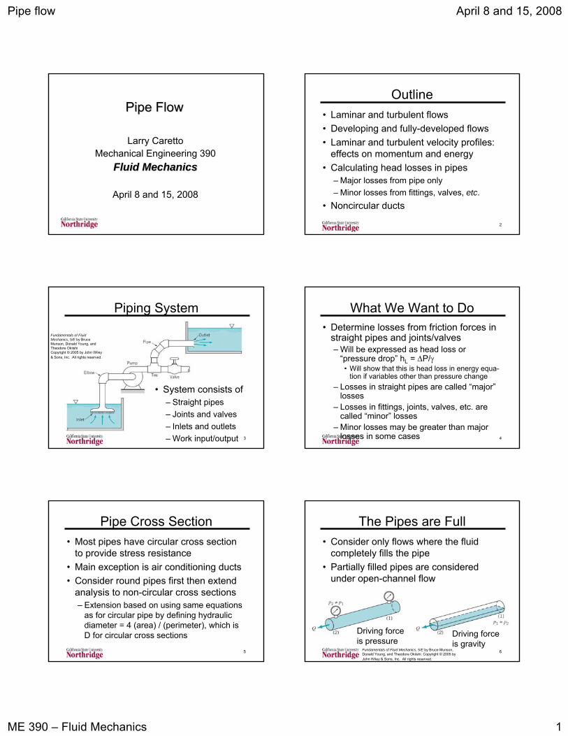
Piping System
• System consists of– Straight pipes– Joints and valves– Inlets and outlets– Work input/output
Fundamentals of Fluid Mechanics, 5/E by Bruce Munson, Donald Young, and Theodore OkiishiCopyright © 2005 by John Wiley & Sons, Inc. All rights reserved.
4
What We Want to Do• Determine losses from friction forces in
straight pipes and joints/valves– Will be expressed as head loss or
“pressure drop” hL = ΔP/γ• Will show that this is head loss in energy equa-
tion if variables other than pressure change– Losses in straight pipes are called “major”
losses– Losses in fittings, joints, valves, etc. are
called “minor” losses– Minor losses may be greater than major
losses in some cases
5
Pipe Cross Section• Most pipes have circular cross section
to provide stress resistance• Main exception is air conditioning ducts• Consider round pipes first then extend
analysis to non-circular cross sections– Extension based on using same equations
as for circular pipe by defining hydraulic diameter = 4 (area) / (perimeter), which is D for circular cross sections
6
The Pipes are Full• Consider only flows where the fluid
completely fills the pipe• Partially filled pipes are considered
under open-channel flow
Driving force is gravity
Driving force is pressure
Fundamentals of Fluid Mechanics, 5/E by Bruce Munson, Donald Young, and Theodore Okiishi. Copyright © 2005 by John Wiley & Sons, Inc. All rights reserved.
Pipe flow April 8 and 15, 2008
ME 390 – Fluid Mechanics 2
7
Laminar vs. Turbulent Flow
• Laminar flows have smooth layers of fluid • Turbulent flows
have fluctuationsFundamentals of Fluid Mechanics, 5/E by Bruce Munson, Donald Young, and Theodore Okiishi. Copyright © 2005 by John Wiley & Sons, Inc. All rights reserved.
8
Laminar vs. Turbulent Flow II• Most flows of engineering interest are
turbulent– Analysis relies mainly on experimentation
guided by dimensional analysis– Even advanced computer models, called
computational fluid dynamics (CFD) rely on “turbulence models” that have large degree of empiricism
• Can get some (very limited) analytical results for laminar flows
9
Laminar vs. Turbulent Flow III• Condition of flow as laminar or turbulent
depends on Reynolds number• For pipe flows
– Re = ρVD/μ < 2100 is laminar– Re = ρVD/μ > 4000 is turbulent– 2100 < Re < 4000 is transition flow
• Other flow geometries have different characteristics in Re = ρVLc/μ and different values of Re for laminar and turbulent flow limits
10
Flow Development
Fundamentals of Fluid Mechanics, 5/E by Bruce Munson, Donald Young, and Theodore Okiishi. Copyright © 2005 by John Wiley & Sons, Inc. All rights reserved.
11
Developing Flows• Entrance regions and bends create
changing flow patters with different head losses
• Once flow is “fully developed” the head loss is proportional to the distance
• Entrance pressure drop is complex– Complete entrance region treated under
minor losses– Will not treat partial entrance region here
12
Developing Flows II• Entrance regions and bends create
changing flow patters with different head losses
• Once flow is “fully developed” the head loss is proportional to the distance
Fundamentals of Fluid Mechanics, 5/E by Bruce Munson, Donald Young, and Theodore Okiishi. Copyright © 2005 by John Wiley & Sons, Inc. All rights reserved.

Pipe flow April 8 and 15, 2008
ME 390 – Fluid Mechanics 3
13
Developing Flows III• After development region, pressure
drop (head loss) is proportional to pipe length
• Equations for entrance region length, ℓe
– Laminar flow:
– Turbulent flow:
– Turbulent flow rule of thumb ℓe ≈ 10D
Re06.0=Del
61Re4.4=Del
14
Fluid Element in Pipe Flow
• Look at arbitrary element, with length ℓ, and radius r, in fully developed flow
• What are forces on this element?Fundamentals of Fluid Mechanics, 5/E by Bruce Munson, Donald Young, and Theodore Okiishi. Copyright © 2005 by John Wiley & Sons, Inc. All rights reserved.
15
Fully Developed Flow
• Pressure drop is due to viscous stresses
( ) 0212
12 =−Δ−−=∑ lrpprprFx πτππ
Flow Direction
rp lτ=Δ
2
Fundamentals of Fluid Mechanics, 5/E by Bruce Munson, Donald Young, and Theodore Okiishi. Copyright © 2005 by John Wiley & Sons, Inc. All rights reserved.
No change in momentum
16
Extend Relation to Wall
• Have Δp = 2τℓ/r for any r: 0 < r < R = D/2• For wall r = R = D/2 and τ = τw = wall
shear stress: Δp = 2τwℓ/R = 4τwℓ/DFundamentals of Fluid Mechanics, 5/E by Bruce Munson, Donald Young, and Theodore Okiishi. Copyright © 2005 by John Wiley & Sons, Inc. All rights reserved.
17
Fully Developed Laminar Flow• Can get
exact equation for pressure drop
4128
DQp
πμ
=Δl
⎥⎥⎦
⎤
⎢⎢⎣
⎡⎟⎠⎞
⎜⎝⎛−=
2
1Rruu c
• Laminar velocity profile
Fundamentals of Fluid Mechanics, 5/E by Bruce Munson, Donald Young, and Theodore Okiishi. Copyright © 2005 by John Wiley & Sons, Inc. All rights reserved.
R
uc
18
Fully Developed Laminar Flow II
⎥⎥⎦
⎤
⎢⎢⎣
⎡⎟⎠⎞
⎜⎝⎛−=
2
1Rruu c
• Laminar shear stress profile found from
Fundamentals of Fluid Mechanics, 5/E by Bruce Munson, Donald Young, and Theodore Okiishi. Copyright © 2005 by John Wiley & Sons, Inc. All rights reserved.
R
rD
uR
rudrdu c
c 2282 μ
=μ=μ=τdrdu
μ=τ
Pipe flow April 8 and 15, 2008
ME 390 – Fluid Mechanics 4
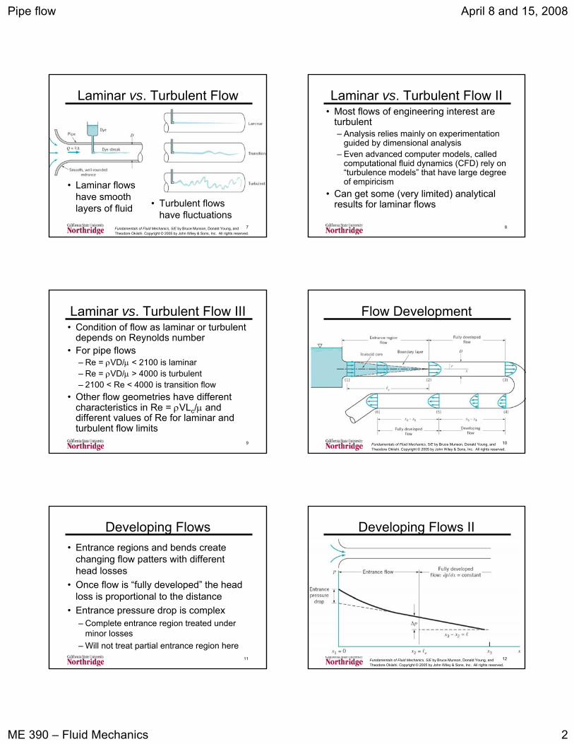
19
Fully Developed Laminar Flow III
∫∫∫ π⎥⎥⎦
⎤
⎢⎢⎣
⎡⎟⎠⎞
⎜⎝⎛−=π==π==
R
c
R
A
rdrRrurdruudARVVAQ
0
2
0
2 212
• What is centerline velocity, uc?
42
4222
2
02
42
0 02
3 RuRrrudr
RrrdruQ c
R
c
R R
c π=⎥⎥⎦
⎤
⎢⎢⎣
⎡−π=
⎥⎥⎦
⎤
⎢⎢⎣
⎡−π= ∫ ∫
VRRV
RVA
RQuRuQ cc 2222
2 2
2
22
2=
ππ
=π
=π
=⇒π=
Centerline uc is twice the mean velocity, V 20
Effect of Velocity Profile• Momentum and kinetic energy flow for
mean velocity, V– FlowMomentum = V = ρVAV = ρV2(πR2)– FlowKE = V2/2 = ρVAV2/2 = ρV3(πR2)/2
• Accurate representation uses profile
m&
m&
AVrdrRruudAuFlow
R
cA
Momentum2
0
2
2
2
3421 ρ=π
⎥⎥⎦
⎤
⎢⎢⎣
⎡⎟⎟⎠
⎞⎜⎜⎝
⎛−ρ=ρ= ∫∫
2221
21
2
3
0
3
2
22 VArdrRruuudAFlow
R
cA
KE ρ=π⎥⎥⎦
⎤
⎢⎢⎣
⎡⎟⎟⎠
⎞⎜⎜⎝
⎛−ρ=ρ= ∫∫
21
Turbulent Flow• For laminar and turbulent flows, the
velocity at the wall is zero– This is called the no-slip condition– Momentum is maximum in the center of the
flow and zero at the wall• Laminar flows: momentum transport from wall
to center is by viscosity, τ = μdu/dr• Turbulent flows: random fluctuations exchange
eddies of high momentum from the center with low momentum flow from near-wall regions
22
Turbulent Flow Quantities
Fundamentals of Fluid Mechanics, 5/E by Bruce Munson, Donald Young, and Theodore Okiishi. Copyright © 2005 by John Wiley & Sons, Inc. All rights reserved.
Velocities at one point as a function of time
u(t) = instantaneous velocityu’ = velocity fluctuation = u –
∫+
=Tt
t
dttuT
u0
0
)(1
u
23
Momentum Exchange
Laminar flow –random molecular motion
Turbulent flow –eddies have structure
Fundamentals of Fluid
Mechanics, 5/E by Bruce
Munson, Donald Young, and
Theodore Okiishi.
Copyright ©2005 by John Wiley & Sons, Inc. All rights
reserved.
Fundamentals of Fluid Mechanics, 5/E by Bruce Munson, Donald Young, and Theodore Okiishi. Copyright © 2005 by John Wiley & Sons, Inc. All rights reserved.
24
Turbulence Regions/Profiles
• Very thin viscous sublayer next to wall– 0.13% of R = 3 in for H20 at = 5 ft/s
• Flat velocity profile in center of flow
( )drud
η+μ=τ
turbulent eddy
viscosity, η
u
Fundamentals of Fluid Mechanics, 5/E by Bruce Munson, Donald Young, and Theodore Okiishi. Copyright © 2005 by John Wiley & Sons, Inc. All rights reserved.

Pipe flow April 8 and 15, 2008
ME 390 – Fluid Mechanics 5
25
Profilen
c Rr
Vu 1
1 ⎟⎠⎞
⎜⎝⎛ −=
Turbulent velocity profiles with n a
function of Reynolds number
n = 6: Re = 1.5x10⁴; Vc/V = 1.264n = 8: Re = 4x10⁵; Vc/V = 1.195
n = 10: Re = 3x10⁶; Vc/V = 1.155Laminar: Vc/V = 2 V = Q/A
Fundamentals of Fluid Mechanics, 5/E by Bruce Munson, Donald Young, and Theodore Okiishi. Copyright © 2005 by John Wiley & Sons, Inc. All rights reserved.
26
Effect of Velocity Profile• Analysis similar to one used for laminar
flow profile– Determine momentum and kinetic energy
flow for mean velocity– Correction factor multiplies average V
results to give integrated u2 and u3 values
1.0311.0113x106101.0461.0164x10581.0771.0271.5x1046
KEMomentumRen
27
Pipe Roughness• Effect of rough walls on pressure drop
may depend on surface roughness of pipe
• Typical roughness values for different materials expressed as roughness length, ε, with units of feet or meters
• Only turbulent flows depend on roughness length, laminar flows do not
28
Pipe roughness effects in viscous sublayer affects pressure drop in turbulent flow
No effect on laminar flow
Fundamentals of Fluid Mechanics, 5/E by Bruce Munson, Donald Young, and Theodore Okiishi. Copyright © 2005 by John Wiley & Sons, Inc. All rights reserved.
29
Use this table (p 433 of text) to find ε
Fundamentals of Fluid Mechanics, 5/E by Bruce Munson, Donald Young, and Theodore Okiishi. Copyright © 2005 by John Wiley & Sons, Inc. All rights reserved.
30
Energy Equation• Energy equation between inlet (1) and
outlet (2)
Ls hhg
Vpzg
Vpz −++γ
+=+γ
+22
211
1
222
2
• Previous applications allowed us to compute the head loss from all other data in this equation– Call this the measured head loss
• We can compute it, but we have no way of knowing its cause
Pipe flow April 8 and 15, 2008
ME 390 – Fluid Mechanics 6
31
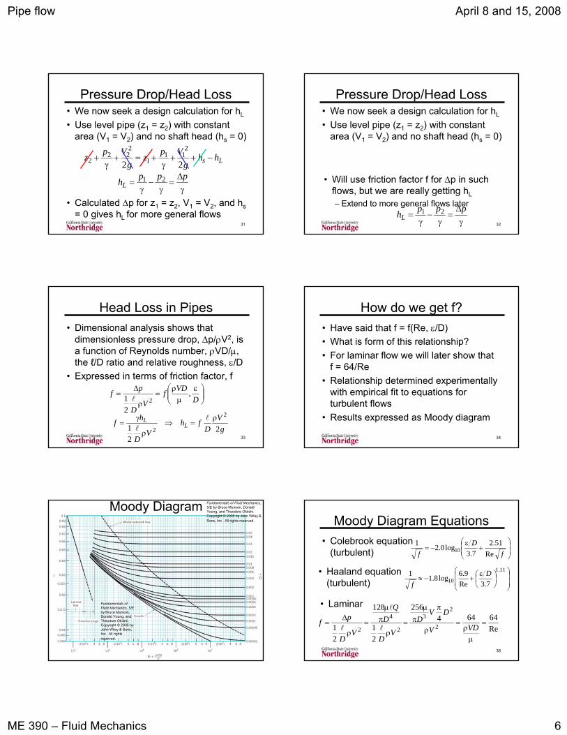
Pressure Drop/Head Loss• We now seek a design calculation for hL
• Use level pipe (z1 = z2) with constant area (V1 = V2) and no shaft head (hs = 0)
γΔ
=γ
−γ
=ppphL
21
• Calculated Δp for z1 = z2, V1 = V2, and hs= 0 gives hL for more general flows
Ls hhg
Vpzg
Vpz −++γ
+=+γ
+22
211
1
222
2
32
Pressure Drop/Head Loss• We now seek a design calculation for hL
• Use level pipe (z1 = z2) with constant area (V1 = V2) and no shaft head (hs = 0)
γΔ
=γ
−γ
=ppphL
21
• Will use friction factor f for Δp in such flows, but we are really getting hL– Extend to more general flows later
33
Head Loss in Pipes• Dimensional analysis shows that
dimensionless pressure drop, Δp/ρV2, is a function of Reynolds number, ρVD/μ, the ℓ/D ratio and relative roughness, ε/D
• Expressed in terms of friction factor, f
⎟⎟⎠
⎞⎜⎜⎝
⎛ εμ
ρ=
ρ
Δ=
DVDf
VD
pf ,
21 2l
gV
Dfh
VD
hf LL
221
2
2
ρ=⇒
ρ
γ=
l
l34
How do we get f?• Have said that f = f(Re, ε/D)• What is form of this relationship?• For laminar flow we will later show that
f = 64/Re• Relationship determined experimentally
with empirical fit to equations for turbulent flows
• Results expressed as Moody diagram
35
Moody Diagram
Fundamentals of Fluid Mechanics, 5/E by Bruce Munson, Donald Young, and Theodore Okiishi. Copyright © 2005 by John Wiley & Sons, Inc. All rights reserved.
Fundamentals of Fluid Mechanics, 5/E by Bruce Munson, Donald Young, and Theodore Okiishi. Copyright © 2005 by John Wiley & Sons, Inc. All rights reserved.
36
Moody Diagram Equations• Colebrook equation
(turbulent) ⎟⎟⎠
⎞⎜⎜⎝
⎛+
ε−=
fD
f Re51.2
7.3log0.21
10
• Laminar
Re64644
256
21
128
21 2
23
2
4
2=
μρ
=ρ
ππ
μ
=ρ
πμ
=ρ
Δ= VDV
DVD
VD
DQ
VD
pfl
l
l
• Haaland equation (turbulent) ⎟
⎟
⎠
⎞
⎜⎜
⎝
⎛⎟⎠⎞
⎜⎝⎛ ε+−≈
11.1
10 7.3Re9.6log8.11 D
f

Pipe flow April 8 and 15, 2008
ME 390 – Fluid Mechanics 7
37
Wholly Turbulent Flows• Large Reynolds numbers: f independent
of Re depends only on ε/D
4
2
22
2
2 16
42 D
QVD
QAQVV
Dfp
π=⇒
π==
ρ=Δ
l
5
2
25
2
24
2
22 8816
22 Dmf
DQf
DQ
DfV
Dfp
ρπ=
ρπ
=π
ρ=
ρ=Δ
&llll
• Pressure drop varies as D-5
– Similar to D-4 dependence in laminar flow
38
Pressure Drop Problems• Find the pressure drop given fluid data,
pipe dimensions, ε, and flow (volume flow, mass flow, or velocity)– Get A = πD2/4– Get V = Q/A or V = /ρA if not given V– Find ρ and μ for fluid at given T and P– Compute Re = ρVD/μ and ε/D– Find f from diagram or equation
• Laminar f = 64/Re; Colebrook for turbulent– Compute Δp = f (ℓ/D) ρV2/2
m&
39
Sample Problem• You have been asked to size a pump
for an airport fuel delivery system. JP-4 fuel (ρ = 1.50 slug/ft3, μ = 1.2x10⁻⁵
slug/ft·s) has to travel 0.5 mi through commercial steel, schedule 40 pipe with a nominal 6 in diameter. The flow rate is 5 slug/s. What is the head loss?
• Schedule 40 pipe: OD = 6.625 in; thickness = 0.280 in; ID = 6.065 in
40
Sample Problem Solution( ) ( ) 222 2006.05054.0
445054.0
12065.6 ftftDAft
inftinD =
π=
π===
( ) sft
ftftslug
sslug
AmV 61.16
2006.050.1
5
33
==ρ
=&
( )41001005.1
102.1
5054.061.1650.1
Re 65
3>=
⋅
=μ
ρ= − x
sftslugx
fts
ftftslug
VD
Since Re > 4,100, flow is turbulent
41
Sample Problem Solution II000297.0
5054.000015.0
==ε
ftft
Dε = 0.00015 for commercial steel (Table 8.1, page 433)
0155.0)000297.0,1005.1(Re 6 ==ε= Dxf
Check f value with Colebrook equation
Find f from Moody diagram (page 434)
⎟⎟⎠
⎞⎜⎜⎝
⎛+−=⎟
⎟⎠
⎞⎜⎜⎝
⎛+
ε−=
0155.01005.151.2
7.3000297.0log0.2
Re51.2
7.3log0.21
61010 xfD
f
0156.0005.81005.81
2 ==⇒= ff
Use f = 0.0156 42
Sample Problem Solution III22
3
2 61.16150.152805054.0
5.02
0156.02
⎟⎠⎞
⎜⎝⎛
⋅
⋅=
ρ=Δ
sft
ftslugslb
ftslug
mift
ftmiV
DfP fl
psiin
lb
ft
lbP ff 2.117
2.1171687622 ===Δ
• For shaft head to overcome this lead loss
ρΔ
≥⇒ρΔ
=γΔ
=≥=PmW
gPPhh
gm
W
innetshaftLs
innetshaft
&&&
&
hplbftshp
ftslug
ft
lbs
slugPmW
f
f
innetshaft 102
55050.1
168765
3
2=
⋅⋅
=ρΔ
≥&&
Pipe flow April 8 and 15, 2008
ME 390 – Fluid Mechanics 8
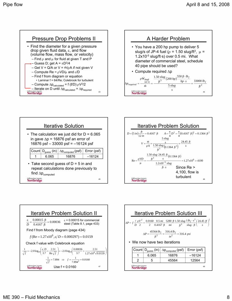
43
Pressure Drop Problems II• Find the diameter for a given pressure
drop given fluid data, ε, and flow (volume flow, mass flow, or velocity)– Find ρ and μ for fluid at given T and P– Guess D; get A = πD2/4– Get V = Q/A or V = /ρA if not given V– Compute Re = ρVD/μ and ε/D– Find f from diagram or equation
• Laminar f = 64/Re; Colebrook for turbulent– Compute Δpcalculated = f (ℓ/D) ρV2/2– Iterate on D until Δpcalculated = Δprequired
m&
44
A Harder Problem• You have a 200 hp pump to deliver 5
slug/s of JP-4 fuel (ρ = 1.50 slug/ft3, μ = 1.2x10⁻⁵ slug/ft·s) over 0.5 mi. What diameter of commercial steel, schedule 40 pipe should be used?
• Compute required Δp
( )2
3 330005
55020050.1
ft
lb
sslug
shplbft
hpftslug
m
Wp f
f
innetshaft
required =⋅
⋅
=
ρ
=Δ&
&
45
Iterative Solution• The calculation we just did for D = 6.065
in gave Δp = 16876 psf an error of 16876 psf – 33000 psf = –16124 psf
1Count
–16124168766.065Error (psf)Δpcomputed (psf)Dguess (in)
• Take second guess of D = 5 in and repeat calculations done previously to find Δpcomputed
46
Iterative Problem Solution( ) ( ) 222 1364.04167.0
444167.0
125 ftftDAft
inftinD =
π=
π===
( ) sft
ftftslug
sslug
AmV 45.24
1364.050.1
5
33
==ρ
=&
( )41001027.1
102.1
1364.045.2450.1
Re 65
3>=
⋅
=μ
ρ= − x
sftslugx
fts
ftftslug
VD
Since Re > 4,100, flow is turbulent
47
Iterative Problem Solution II00036.0
4167.000015.0
==ε
ftft
Dε = 0.00015 for commercial steel (Table 8.1, page 433)
0159.0)000297.0,1027.1(Re 6 ==ε= Dxf
Check f value with Colebrook equation
Find f from Moody diagram (page 434)
⎟⎟⎠
⎞⎜⎜⎝
⎛+−=⎟
⎟⎠
⎞⎜⎜⎝
⎛+
ε−=
0159.01027.151.2
7.300036.0log0.2
Re51.2
7.3log0.21
61010 xfD
f
0160.0894.71894.71
2 ==⇒= ff
Use f = 0.0160 48
Iterative Problem Solution III22
3
2 45.24150.152804167.0
5.02
0160.02
⎟⎠⎞
⎜⎝⎛
⋅
⋅=
ρ=Δ
sft
ftslugslb
ftslug
mift
ftmiV
DfP fl
psiin
lb
ft
lbP ff 4.316
4.3164556422 ===Δ
• We now have two iterations
1256445564521
Count–16124168766.065
Error (psf)Δpcomputed (psf)Dguess (in)
Pipe flow April 8 and 15, 2008
ME 390 – Fluid Mechanics 9
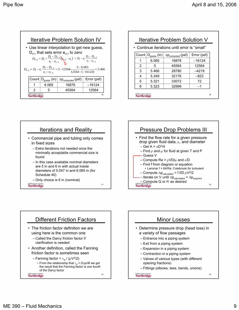
49
Iterative Problem Solution IV• Use linear interpolation to get new guess,
Di+1 that sets error ei+1 to zero
1256445564521
Count–16124168766.065
Error (psf)Δpcomputed (psf)Dguess (in)
( )iiii
iiii ee
eeDDDD −
−−
+= +−
−+ 1
1
11
( ) 466.51612412564
065.651256451
11 =
−−−
−=−−
−=−
−+
ii
iiiii ee
DDeDD0
1
1
−
−
−−
−=ii
iiii ee
DDeD
50
Iterative Problem Solution V• Continue iterations until error is “small”
–1329995.323672330725.3215
–823321765.3494–4219287805.4663125644556452
1Count
–16124168766.065Error (psf)Δpcomputed (psf)Dguess (in)
51
Iterations and Reality• Commercial pipe and tubing only comes
in fixed sizes– Extra iterations not needed once the
minimally acceptable commercial size is found
– In this case available nominal diameters are 5 in and 6 in with actual inside diameters of 5.047 in and 6.065 in (for Schedule 40)
– Only choice is 6 in (nominal)52
Pressure Drop Problems III• Find the flow rate for a given pressure
drop given fluid data, ε, and diameter– Get A = πD2/4– Find ρ and μ for fluid at given T and P– Guess V– Compute Re = ρVD/μ and ε/D– Find f from diagram or equation
• Laminar f = 64/Re; Colebrook for turbulent– Compute Δpcalculated = f ℓ/D ρV2/2– Iterate on V until Δpcalculated = Δprequired– Compute Q or as desiredm&
53
Different Friction Factors• The friction factor definition we are
using here is the common one– Called the Darcy friction factor if
clarification is needed• Another definition, called the Fanning
friction factor is sometimes seen– Fanning factor = τw / (ρV2/2)
• From the relationship that τw = DΔp/4ℓ we get the result that the Fanning factor is one fourth of the Darcy factor
54
Minor Losses• Determine pressure drop (head loss) in
a variety of flow passages– Entrance into a piping system– Exit from a piping system– Expansion in a piping system– Contraction in a piping system– Valves of various types (with different
opening fractions)– Fittings (elbows, tees, bends, unions)

Pipe flow April 8 and 15, 2008
ME 390 – Fluid Mechanics 10
55
Minor Losses• Fittings in pipe systems modeled as
loss coefficients, KL
222
222 VKpg
VKgp
gVKh LLL
LLL
ρ=Δ⇒=
ρΔ
⇒=
• KL depends on geometry and Re– For flows dominated by inertia effects KL is
a function of geometry only• Alternative process, not given here,
uses equivalent length for minor losses56
Entrance Losses
Reentrant: KL = 0.8
Sharp edged: KL = 0.5
Slightly rounded: KL = 0.2 Well rounded:
KL = f(r/D)
r
D
2
2VKp LLρ
=Δ V = Pipe velocity
Fundamentals of Fluid Mechanics, 5/E by Bruce Munson, Donald Young, and Theodore Okiishi. Copyright © 2005 by John Wiley & Sons, Inc. All rights reserved.
57
Rounded Inlet KL
Fundamentals of Fluid Mechanics, 5/E by Bruce Munson, Donald Young, and Theodore Okiishi. Copyright © 2005 by John Wiley & Sons, Inc. All rights reserved.
Slightly rounded KL= 0.2 for r/D = 0.055
r/D = 0 is square inlet
58
Full KE loss cannot be recovered in sharp-edged entrance
Fundamentals of Fluid Mechanics, 5/E by Bruce Munson, Donald Young, and Theodore Okiishi. Copyright © 2005 by John Wiley & Sons, Inc. All rights reserved.
59
KL = 1 for all exit flows
Reentrant
Slightly rounded
Sharp edged
Well rounded
Fundamentals of Fluid Mechanics, 5/E by Bruce Munson, Donald Young, and Theodore Okiishi. Copyright © 2005 by John Wiley & Sons, Inc. All rights reserved.
60
New AreaSudden contraction (left)
For sudden expansion (right) KL = ( 1 –A1/A2)2

Pipe flow April 8 and 15, 2008
ME 390 – Fluid Mechanics 11
61
Fundamentals of Fluid Mechanics, 5/E by Bruce Munson, Donald Young, and Theodore Okiishi. Copyright © 2005 by John Wiley & Sons, Inc. All rights reserved.
62
Fundamentals of Fluid Mechanics, 5/E by Bruce Munson, Donald Young, and Theodore Okiishi. Copyright © 2005 by John Wiley & Sons, Inc. All rights reserved.
63
Problem with Minor Losses• 4 kg/s of oil with SG = 0.82 and μ = 0.05
kg·m/s2 is pumped from one tank to another. The line of 2-in Schedule-40 pipe has a total length of 40 m, with two gate valves and six elbows (regular flanged 90o). The entrance is rounded with an r/D ratio of 0.1.
• Find pressure loss with both valves open• 2-in schedule 40 pipe has OD = 2.375 in
and thickness = 0.154 in, so ID = 2.067 in = 0.05250 m
64
Problem Solution( )
2
22
002165.0
05250.044
m
mDA
=
π=
π=
( ) sm
mm
kgskg
AmV 26.2
002165.02.819
4
33
==ρ
=&
( )21001940050.0
05250.026.22.819
Re3
<=
⋅
=μ
ρ=
smkg
ms
mm
kgVD
Since Re < 2,100, flow is laminar
( )
skg
skg
SG ref2.819999)82.0( =
=ρ=ρ
65
Problem Solution IIFind Δpmajor directly from laminar flow equation
( ) ( )
( )kPa
mN
ms
mmm
sN
DQpmajor 369.5252369
05250.0
004883.04005.012812824
3
2
4 ==π
⋅
=πμ
=Δl
sm
kgm
skgmQ
33 04883.02.819
4==
ρ=&
Minor losses coefficients: rounded entrance (r/D = 0.1), KL = 0.12; exit, KL = 1; fully open gate valve, KL = 0.15; 6 elbows, KL = 6(0.3) = 1.8. Total KL = 0.12 + 1 + 0.15 + 1.8 = 3.07
Could also use f = 64/Re
66
Problem Solution IIIΔpminor = (Loss coefficient sum) times ρV2/2
( ) 2
22
3
2 397,6126.2819207.3
2 mN
mkgsN
sm
mkgVKp L =
⋅⋅
⎟⎠⎞
⎜⎝⎛=
ρ=Δ ∑minor
22397,6369,52m
Nm
Nppp majortotal +=Δ+Δ=Δ minor
kPam
Nptotal 8.58766,582 ==Δ

Pipe flow April 8 and 15, 2008
ME 390 – Fluid Mechanics 12
67
Noncircular Ducts• Define hydraulic diameter, Dh = 4A/P
– A is cross-sectional area for flow– P is wetted perimeter– For a circular pipe where A = πD2/4 and P
= πD, Dh = 4(πD2/4) / (πD) = D• For turbulent flows use Moody diagram
with D replaced by Dh in Re, f, and ε/D• For laminar flows, f = C/Re (both based
on Dh) – see next slide for C values68
2
2VD
fPh
ρ=Δ
l
PADh
4=
μρ
=VD
hRe
Fundamentals of Fluid Mechanics, 5/E by Bruce Munson, Donald Young, and Theodore Okiishi. Copyright © 2005 by John Wiley & Sons, Inc. All rights reserved.
42
hDQCP lμ
π=Δ
69
Problem• An 10-in-square, commercial steel air
conditioning duct contains air at 80oF and atmospheric pressure and has a flow rate of 125 ft3/min. Find the pressure drop per unit duct length
• Property data at 80oF (Table B.3) ρ = 0.002286 slug/ft3; ν = 1.69x10⁻⁴ ft2/s
• Solution: find Reh to see if flow is laminar or turbulent then find f and Δp
70
Solution
ftin
LLL
PADh
8333.010444 2
==
===
( )5
24 1078.11069.1
8333.03
Re x
sftx
ftsft
VDhh ==
ν= −
( ) sft
inftin
sft
AQV 3
14410
60min
min125
2
22
3
===
00018.08333.000015.0
==ε
ftft
Dε = 0.00015 for commercial steel (Table 8.1, page 433)
Turbulent flow for Reh > 4100
71
Solution II
0172.0)00018.0,1027.1(Re 6 ==ε= Dxf
Check f value with Colebrook equation
Find f from Moody diagram (page 434)
⎟⎟⎠
⎞⎜⎜⎝
⎛+−=⎟
⎟⎠
⎞⎜⎜⎝
⎛+
ε−=
0172.01078.151.2
7.300018.0log0.2
Re51.2
7.3log0.21
51010 xfD
f
0173.0611.71611.71
2 ==⇒= ff Use f = 0.0173
3
522
3
2 1078.13100229.08333.0
12
0173.02
1ft
lbxsft
ftslugslb
ftslug
ftV
DfP ff
−
=⎟⎠⎞
⎜⎝⎛
⋅
⋅=
ρ=
Δl
72
Recommended Air Velocity
6.5 - 152.0 - 4.5Ventilation ducts (offices)5.9 - 131.8 - 4Ventilation ducts (hospitals)66 - 9820 - 30Compressed air pipe26 - 498 - 15Vacuum cleaning pipe
2.6 - 3.30.8 - 1.0Warm air for house heating3.3 - 9.81 - 3Air inlet to boiler room40 - 6612 - 20Combustion air ducts
ft/sm/sAir Velocity
Air Ducts
http://www.engineeringtoolbox.com/flow-velocity-air-ducts-d_388.html