Pipelining to SuperscalarECE/CS 752 Fall 2017

Prof. Mikko H. LipastiUniversity of Wisconsin-Madison

Pipelining to Superscalar

• Forecast– Limits of pipelining– The case for superscalar– Instruction-level parallel machines– Superscalar pipeline organization– Superscalar pipeline design

Generic Instruction Processing Pipeline

WR. MEM.

ID

RD

ALU

MEM

WB

1

2

3

4

5

IF

6

I-CACHEPC

DECODE

RD. REG.

ALU OP.

ADDR. GEN.

I-CACHEPC

DECODE

RD. REG.

I-CACHEPC

DECODE

RD. REG.

I-CACHEPC

DECODE

RD. REG.

WR. REG. WR. REG.

IF:

ID:

OF:

EX:

OS:

LOAD STORE BRANCHALU

RD. MEM.

ADDR.GEN. ADDR. GEN.

WR. PC

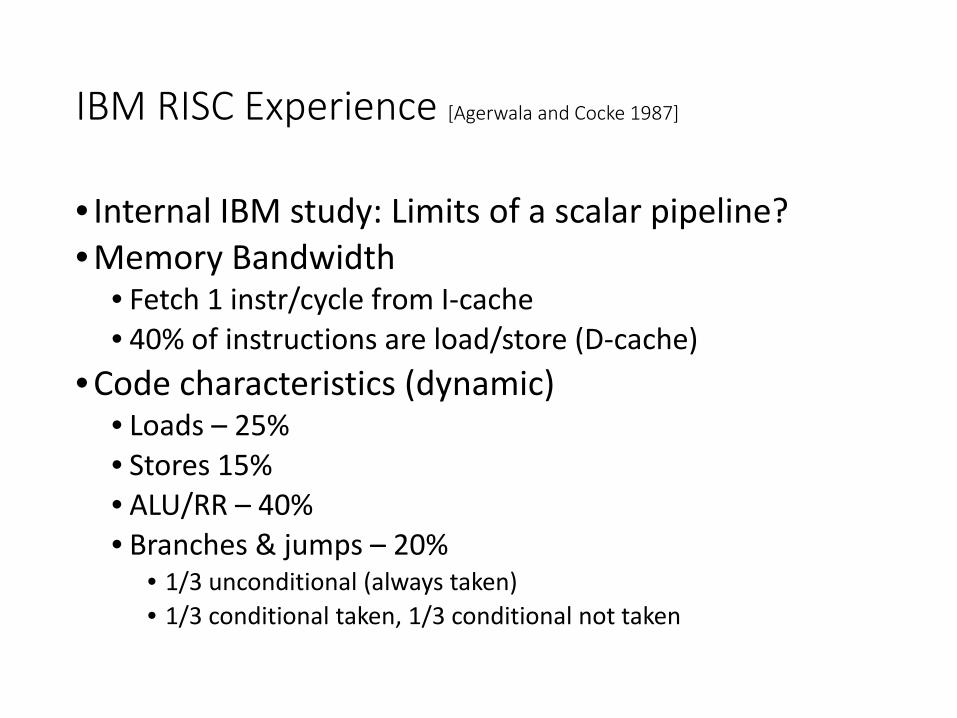
IBM RISC Experience [Agerwala and Cocke 1987]

• Internal IBM study: Limits of a scalar pipeline?• Memory Bandwidth

• Fetch 1 instr/cycle from I-cache• 40% of instructions are load/store (D-cache)

• Code characteristics (dynamic)• Loads – 25%• Stores 15%• ALU/RR – 40%• Branches & jumps – 20%

• 1/3 unconditional (always taken)• 1/3 conditional taken, 1/3 conditional not taken

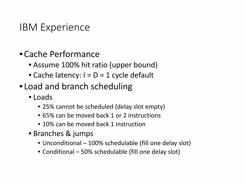
IBM Experience

• Cache Performance• Assume 100% hit ratio (upper bound)• Cache latency: I = D = 1 cycle default

• Load and branch scheduling• Loads

• 25% cannot be scheduled (delay slot empty)• 65% can be moved back 1 or 2 instructions• 10% can be moved back 1 instruction

• Branches & jumps• Unconditional – 100% schedulable (fill one delay slot)• Conditional – 50% schedulable (fill one delay slot)

CPI Optimizations

• Goal and impediments• CPI = 1, prevented by pipeline stalls

• No cache bypass of RF, no load/branch scheduling• Load penalty: 2 cycles: 0.25 x 2 = 0.5 CPI• Branch penalty: 2 cycles: 0.2 x 2/3 x 2 = 0.27 CPI• Total CPI: 1 + 0.5 + 0.27 = 1.77 CPI

• Bypass, no load/branch scheduling• Load penalty: 1 cycle: 0.25 x 1 = 0.25 CPI• Total CPI: 1 + 0.25 + 0.27 = 1.52 CPI

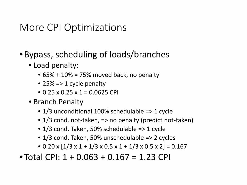
More CPI Optimizations

• Bypass, scheduling of loads/branches• Load penalty:

• 65% + 10% = 75% moved back, no penalty• 25% => 1 cycle penalty• 0.25 x 0.25 x 1 = 0.0625 CPI

• Branch Penalty• 1/3 unconditional 100% schedulable => 1 cycle• 1/3 cond. not-taken, => no penalty (predict not-taken)• 1/3 cond. Taken, 50% schedulable => 1 cycle• 1/3 cond. Taken, 50% unschedulable => 2 cycles• 0.20 x [1/3 x 1 + 1/3 x 0.5 x 1 + 1/3 x 0.5 x 2] = 0.167

• Total CPI: 1 + 0.063 + 0.167 = 1.23 CPI

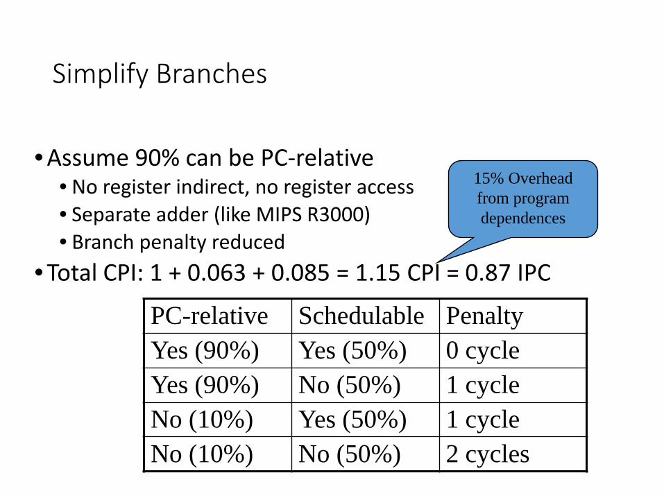
Simplify Branches

• Assume 90% can be PC-relative• No register indirect, no register access• Separate adder (like MIPS R3000)• Branch penalty reduced

• Total CPI: 1 + 0.063 + 0.085 = 1.15 CPI = 0.87 IPC

PC-relative Schedulable PenaltyYes (90%) Yes (50%) 0 cycleYes (90%) No (50%) 1 cycleNo (10%) Yes (50%) 1 cycleNo (10%) No (50%) 2 cycles

15% Overhead from program dependences

Limits of Pipelining

• IBM RISC Experience– Control and data dependences add 15%– Best case CPI of 1.15, IPC of 0.87– Deeper pipelines (higher frequency) magnify dependence penalties

• This analysis assumes 100% cache hit rates– Hit rates approach 100% for some programs– Many important programs have much worse hit rates

– Later!

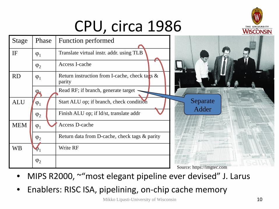
CPU, circa 1986

• MIPS R2000, ~“most elegant pipeline ever devised” J. Larus• Enablers: RISC ISA, pipelining, on-chip cache memory

Mikko Lipasti-University of Wisconsin 10

Stage Phase Function performed

IF φ1 Translate virtual instr. addr. using TLB

φ2 Access I-cache

RD φ1 Return instruction from I-cache, check tags & parity

φ2 Read RF; if branch, generate target

ALU φ1 Start ALU op; if branch, check condition

φ2 Finish ALU op; if ld/st, translate addr

MEM φ1 Access D-cache

φ2 Return data from D-cache, check tags & parity

WB φ1 Write RF

φ2Source: https://imgtec.com

SeparateAdder

Processor Performance

• In the 1980’s (decade of pipelining):– CPI: 5.0 => 1.15

• In the 1990’s (decade of superscalar):– CPI: 1.15 => 0.5 (best case)

• In the 2000’s (decade of multicore):– Focus on thread-level parallelism, CPI => 0.33 (best case)

Processor Performance = ---------------Time

Program

Instructions CyclesProgram Instruction

TimeCycle

(code size)

= X X

(CPI) (cycle time)

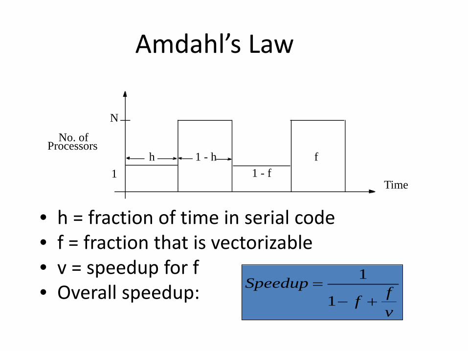
Amdahl’s Law

• h = fraction of time in serial code• f = fraction that is vectorizable• v = speedup for f• Overall speedup:

No. ofProcessors

N

Time1

h 1 - h1 - f

f

vff

Speedup+−

=1

1

Revisit Amdahl’s Law

• Sequential bottleneck• Even if v is infinite

– Performance limited by nonvectorizable portion (1-f)

fvff

v −=

+−∞→ 1

1

1

1lim

No. ofProcessors

N

Time1

h 1 - h1 - f

f

Pipelined Performance Model

• g = fraction of time pipeline is filled• 1-g = fraction of time pipeline is not filled

(stalled)

1-g g

PipelineDepth

N

1

g = fraction of time pipeline is filled 1-g = fraction of time pipeline is not filled

(stalled)

1-g g

PipelineDepth

N

1

Pipelined Performance Model

Pipelined Performance Model

• Tyranny of Amdahl’s Law [Bob Colwell]– When g is even slightly below 100%, a big performance hit

will result– Stalled cycles are the key adversary and must be minimized

as much as possible

1-g g

PipelineDepth

N

1

Motivation for Superscalar[Agerwala and Cocke]

Typical Range

Speedup jumps from 3 to 4.3 for N=6, f=0.8, but s =2 instead

of s=1 (scalar)

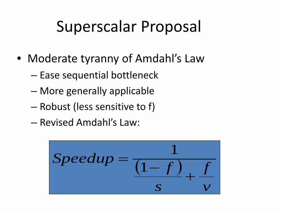
Superscalar Proposal

• Moderate tyranny of Amdahl’s Law– Ease sequential bottleneck– More generally applicable– Robust (less sensitive to f)– Revised Amdahl’s Law:

( )vf

sfSpeedup+

−= 1

1

Limits on Instruction Level Parallelism (ILP)

Weiss and Smith [1984] 1.58Sohi and Vajapeyam [1987] 1.81Tjaden and Flynn [1970] 1.86 (Flynn’s bottleneck)Tjaden and Flynn [1973] 1.96Uht [1986] 2.00Smith et al. [1989] 2.00Jouppi and Wall [1988] 2.40Johnson [1991] 2.50Acosta et al. [1986] 2.79Wedig [1982] 3.00Butler et al. [1991] 5.8Melvin and Patt [1991] 6Wall [1991] 7 (Jouppi disagreed)Kuck et al. [1972] 8Riseman and Foster [1972] 51 (no control dependences)Nicolau and Fisher [1984] 90 (Fisher’s optimism)

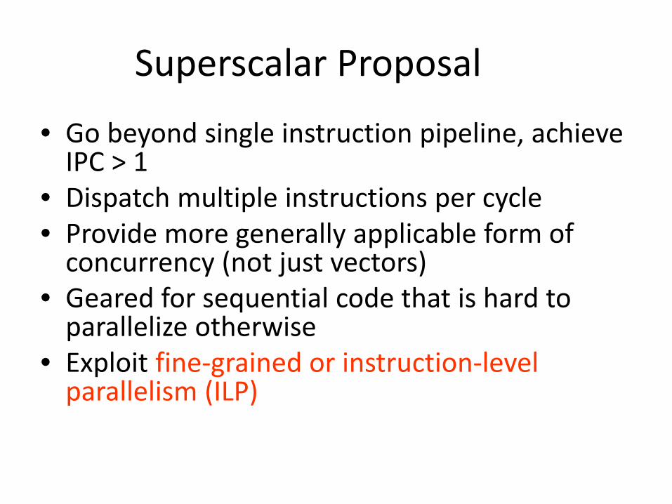
Superscalar Proposal

• Go beyond single instruction pipeline, achieve IPC > 1

• Dispatch multiple instructions per cycle• Provide more generally applicable form of

concurrency (not just vectors)• Geared for sequential code that is hard to

parallelize otherwise• Exploit fine-grained or instruction-level

parallelism (ILP)

Classifying ILP Machines[Jouppi, DECWRL 1991]• Baseline scalar RISC

– Issue parallelism = IP = 1– Operation latency = OP = 1– Peak IPC = 1

12 3 4

5 6

IF DE EX WB

1 2 3 4 5 6 7 8 90

TIME IN CYCLES (OF BASELINE MACHINE)

SUC

CES

SIVE

INST

RU

CTI

ON

S

Classifying ILP Machines[Jouppi, DECWRL 1991]• Superpipelined: cycle time = 1/m of baseline

– Issue parallelism = IP = 1 inst / minor cycle– Operation latency = OP = m minor cycles– Peak IPC = m instr / major cycle (m x speedup?)

12

34

5

IF DE EX WB6

1 2 3 4 5 6

Classifying ILP Machines[Jouppi, DECWRL 1991]• Superscalar:

– Issue parallelism = IP = n inst / cycle– Operation latency = OP = 1 cycle– Peak IPC = n instr / cycle (n x speedup?)

IF DE EX WB

123

456

9

78

Classifying ILP Machines[Jouppi, DECWRL 1991]• VLIW: Very Long Instruction Word

– Issue parallelism = IP = n inst / cycle– Operation latency = OP = 1 cycle– Peak IPC = n instr / cycle = 1 VLIW / cycle

IF DE

EX

WB

Classifying ILP Machines[Jouppi, DECWRL 1991]• Superpipelined-Superscalar

– Issue parallelism = IP = n inst / minor cycle– Operation latency = OP = m minor cycles– Peak IPC = n x m instr / major cycle

IF DE EX WB

123

456

9

78

Superscalar vs. Superpipelined

• Roughly equivalent performance– If n = m then both have about the same IPC– Parallelism exposed in space vs. time

Time in Cycles (of Base Machine)0 1 2 3 4 5 6 7 8 9

SUPERPIPELINED

10 11 12 13

SUPERSCALARKey:

IFetchDcode

ExecuteWriteback

Superpipelining: Result Latency

Superpipelining - Jouppi, 1989

essentially describes a pipelined execution stage

Jouppií s base machine

Underpipelined machine

Superpipelined machine

Underpipelined machines cannot issue instructions as fast as they are executed

Note - key characteristic of Superpipelined machines is that results are not available to M-1 successive instructions

Superscalar Challenges

I-cache

FETCH

DECODE

COMMITD-cache

BranchPredictor Instruction

Buffer

StoreQueue

ReorderBuffer

Integer Floating-point Media Memory

Instruction

RegisterData

MemoryData

Flow

EXECUTE

(ROB)

Flow

Flow