Pipe-It Case Study Multi Field Asset Integrated...

CONTACT ADDRESS TELEPHONE NUMBER COMPANY E‐MAIL

+47 7384 8080 [email protected]

FAX NUMBER CORPORATE WEBSITE

REGISTER OF BUSINEESS ENTERPRISES

Granaasveien 1 7048 Trondheim Norway

+47 7384 8081 www.petrostreamz.com NO 989206230

Pipe-It Case Study Multi‐Field Asset Integrated Optimization Benchmark (SPE 130768)

Field: Extended reservoir model

of Papers SPE 121252 and SPE

16000

Client: Petroleum Industry

Location: EUROPEC 2010

Challenge Solution Benefit Integrated modeling and optimization of multi‐field assets, from subsurface to market.

Provide different application to simulate field asset model and evaluate the optimal production strategies using key control variables.

The benchmark is provided to the industry through application data files, network infrastructure and results.

Summary Integrated modeling of multi‐field assets, from subsurface to market, is challenging due to the

complexity of the problem. This study is an extension of the SPE 121252, model based integration and optimization gas cycling benchmark, extending two gas‐condensate fields to two full‐field multi‐well models and introducing an oil field undergoing miscible WAG injection, where most data are taken from the SPE 5 Reservoir Simulation Comparative Project, SPE 16000.

A common field‐wide surface processing facility is modeled with emphasis on water handling, NGL extraction, sales‐gas spec, and gas reinjection. The surface process model interacts with the three reservoir models through two main mechanisms – (1) water‐ and gas‐handling constraints, and (2) distribution of available produced gas for reinjection into the three reservoirs. The multi‐field asset model is introduced as a benchmark case.

Cost functions are introduced for all major control variables (number of wells, surface facility selection and operating conditions). Net present value is used as the target objective function in the optimization.

Introduction The model presented in this paper is rich and complex enough to represent the value chain

from reservoir to export and thus suitable as a benchmark for integrated operations and optimization. The upstream part of the integrated model includes two gas‐condensate reservoirs

of 17

and an oil reservoir while the surface process system includes gas and liquid separation as well as an NGL plant. The model also includes an economic calculation as indicated in Fig. 1. All model components have been designed using realistic assumptions and parameter values. Further, the project is designed with close links between the upstream and downstream parts of the model, partly due to gas re‐injection. This is important since the integrated model is designed to study and assess the business value of integrated optimization as a decision support method. Complete documentation of the integrated model and optimization is made available at http://www.ipt.ntnu.no/~io‐opt/wiki/doku.php.

Fig. 1. Integrated optimization schematic.

Reservoir Model The reservoir models include two gas‐condensate reservoirs and an oil reservoir, as shown in

Fig. 1. The gas‐condensate reservoirs are scaled up from [Juell, et al., 2010] and the oil reservoir is a scaled up version of a miscible WAG project [Killough and Kossack, 1987]. In the base case each

reservoir is producing through production wells and injection operations are conducted through

injection wells which perform gas injection wells in the gas‐condensate reservoirs and WAG injection in the oil reservoir. The production and injection wells are perforated through all layers. The reservoir models and well locations are shown in Fig. 2.

The size of the gas‐condensate reservoirs is 3218 x 3218 x 48.7 m3 which is divided into 36 x 36 x 4 grid blocks. The oil reservoir size is 5334 x 5334 x 30.48 m3, divided into 35 x 35 x 3 grid blocks. The horizontal permeability distributions for the three reservoirs vary from a low permeability in the south west region towards higher permeability in the north east. The permeability distribution range is presented on Table 1. There are two faults in the horizontal direction, one is sealing and the other is partially communicating. The non‐communicating fault separates low permeability and medium permeability areas. The partially communicating fault separates the medium and high permeability areas. The non‐communicating shale in the vertical direction occurs between layers 3 and 4 in the lean gas‐condensate reservoir, between layers 1 and 2 in the rich gas‐condensate reservoir and between layers 2 and 3 in the oil reservoir. The reservoir models are compositional. The composition for the gas‐condensate reservoirs consists of 9 components and the composition for the oil reservoir consists of 6 components. The initial fluid composition for each reservoir is presented in Table 2. The compositional reservoir models are run using the SENSOR® reservoir simulator.

http://www.ipt.ntnu.no/%7Eio-opt/wiki/doku.php

of 17

Lean

Gas Conden

sate

Sealing fault

PROD 3GINJ 4

GINJ 3

PROD 1

GINJ 1

PROD 2

GINJ 2

GINJ 7PROD 4

GINJ 6

PROD 5

GINJ 8

GINJ 5

Rich Gas Condensate

Sealing fault

PROD 3GINJ 4

GINJ 3

PROD 1

GINJ 1

PROD 2

GINJ 2GINJ 2

GINJ 7PROD 4

GINJ 6

GINJ 8

PROD 5

GINJ 5

Sealing fault

GINJ 7

GINJ 6

GINJ 8

GINJ 5

GINJ 3

GINJ 1GINJ 4

PROD 3

PROD 1

PROD 2

PROD 5Oil

PROD 4

(a). Lean Gas Condensate Reservoir.

(b). Rich Gas Condensate Reservoir. (c). Oil Reservoir.

Fig. 2. Reservoir description; heterogeneity and well placement.

Table 1. Horizontal permeability and thickness distributions.

Lean Gas

Condensate

Rich Gas

CondensateOil

Gas

CondensateOil

1 13‐1300 35‐3500 50‐5000 9.1 6.1

2 4‐400 4.5‐450 5‐500 9.1 9.1

3 2‐200 2.5‐250 20‐2000 15.2 15.2

4 15‐1500 1‐100 ‐ 15.2 ‐

Layer

Permeability (md) Thickness (m)

Table 2. Initial composition for each reservoir.

Layer 1 Layer 2 Layer 3 Layer 4

CO2 0.01195 0.05794 0.05789 0.05777 0.05713

N2 0.01995 0.01852 0.01829 0.01789 0.01655

C1 0.66936 0.62858 0.62398 0.61573 0.58684

C2 0.10868 0.08288 0.0831 0.08347 0.08442

C3 0.06474 0.0564 0.05691 0.05778 0.06048

C4‐6 0.07976 0.09251 0.09382 0.09611 0.10359

C7P1 0.03272 0.04521 0.0469 0.04995 0.06078

C7P2 0.01052 0.01468 0.01543 0.0168 0.02175

C7P3 0.00234 0.00327 0.00367 0.00449 0.00845

C1 C3 C6 C10 C15 C20

0.5 0.03 0.07 0.2 0.15 0.05

ComponentLean GC

Reservoir

Rich GC Reservoir

Oil Reservoir (Component)

Well Vertical Flow Model

The vertical well flow model is integrated into the reservoir simulator by introducing the Tubing Head Pressure table (THP table). The THP table for each well is generated using the PROSPER® simulator. The data range and underlying model that are used to generate the THP table are provided in Table 3.

Surface Pipeline Flow Model

of 17

gas and one transporting liquid, as shown in Fig. 3. The pipeline data is presented in Table 4.

Table 3. Well and Field Properties.

Lean GC Rich GC Oil

Rate (Units) SM3/D SM3/D SM3/D

Min:(Intervals):Max 2831.69:(20):1.42E+06 2831.69:(20):1.42E+06 15.9:(20):3974.68

OGR SM3/SM3 SM3/SM3 GOR (SM3/SM3)

2.8E‐05:(10):3.4E‐03 2.8E‐05:(10):3.4E‐03 53.4:(10):1781.1

WGR SM3/SM3 SM3/SM3 water cut (SM3/SM3)

0 0 0:(10):1

THP Bara Bara Bara

6.89:(10):244.76 6.89:(10):172.36 6.89:(10):344.73

in in in

0.11 0.11 0.13

Well Depth m m m

7425 7425 8425

SM3/D SM3/D SM3/D

5.4 E+05 5.4 E+05 1920

Bara Bara Bara

68.95 68.95 68.95

Bara Bara Bara

275.8 275.8 310.3

SM3/D SM3/D SM3/D

2.7 E+06 2.7 E+06 9600

Maximum Plateau

Rate Target

Tubing Inside

Diameter

Maximum Producer

Rate Constraint

Minimum Producer

THP Constraint

Maximum Injector

BHP Constraint

ParameterReservoir

Table 4. Surface pipeline properties.

Lean GC Rich GC Oil

Length km 5 10 11.5

Inner Diameter m 0.254 0.254 0.3048

Roughness mm 4.60E‐02 4.60E‐02 4.60E‐02

Parameter UnitReservoir

Surface Process Model The surface model is a steady state model where input streams will vary with time since these

inputs are determined by the reservoir models. The surface process model is implemented in HYSYS. The surface process model is separated into two main separation processes, liquid and gas

separation. The liquid separation process consists of multi‐stage separation processes. Separators

and are three‐phase separation processes which separates gas, oil and water. Separators and

are two‐phase separation processes which separates gas and liquid. Further, there is a second‐step drying stage for each separator to extract more liquid from the separated gas stream. The final product from the liquid separation process is condensate. A water pump is installed to transfer water to the water disposal facility.

of 17

plant; each process is simplified by representing it by a splitter model. In the real field separation process, complex unit operations are required such as distillation columns in a NGL plant. The Dew Point Controller (DPC) unit is installed to produce high NGL recovery. There are six final products from the gas separation process facility. These are sales gas, fuel gas, re‐injected gas to the lean gas‐condensate reservoir, re‐injected gas to the rich gas‐condensate reservoir, re‐injected gas to the oil reservoir and NGL. There are two products from the NGL plant, NGL vapor and NGL liquid. NGL vapor mainly consists of methane, ethane and propane and will be re‐injected to the oil reservoir while NGL liquid mainly consists of heavy components which will be sold as NGL. The surface process plant architecture is presented in Fig. 3.

Fig. 3. Surface process facility schematic.

Thermodynamic Model Peng‐Robinson 1979 (PR‐1979) was used as the EOS model in the HYSYS, PROSPER and SENSOR

simulators.

Economic Model The goal of the integrated model is to study field asset value as represented by an economic

model. This model is based on Net Present Value (NPV), with introducing a discount factor. The operational expenses (OPEX) cover the surface and well operation and are defined by a fixed

amount, one million USD per day for the base case. The field revenue is obtained from gas (

USD/m3), NGL and condensate sales ( USD/m3). The daily cost is summed from the volume of

of 17

water production and injection ( USD/m3), CO2 removal ( USD/MT) and power

consumption ( cents/kWh).

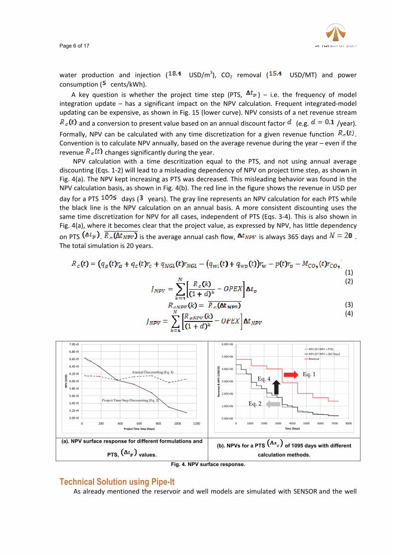
A key question is whether the project time step (PTS, ) – i.e. the frequency of model integration update – has a significant impact on the NPV calculation. Frequent integrated‐model updating can be expensive, as shown in Fig. 15 (lower curve). NPV consists of a net revenue stream

and a conversion to present value based on an annual discount factor (e.g. /year).

Formally, NPV can be calculated with any time discretization for a given revenue function . Convention is to calculate NPV annually, based on the average revenue during the year – even if the

revenue changes significantly during the year. NPV calculation with a time descritization equal to the PTS, and not using annual average

discounting (Eqs. 1‐2) will lead to a misleading dependency of NPV on project time step, as shown in Fig. 4(a). The NPV kept increasing as PTS was decreased. This misleading behavior was found in the NPV calculation basis, as shown in Fig. 4(b). The red line in the figure shows the revenue in USD per

day for a PTS days ( years). The gray line represents an NPV calculation for each PTS while the black line is the NPV calculation on an annual basis. A more consistent discounting uses the same time discretization for NPV for all cases, independent of PTS (Eqs. 3‐4). This is also shown in Fig. 4(a), where it becomes clear that the project value, as expressed by NPV, has little dependency

on PTS . is the average annual cash flow, is always 365 days and . The total simulation is 20 years.

(1)

(2)

(3)

(4)

5.0E+9

5.2E+9

5.4E+9

5.6E+9

5.8E+9

6.0E+9

6.2E+9

6.4E+9

6.6E+9

6.8E+9

7.0E+9

0 200 400 600 800 1000 1200

NPV (USD

)

Project Time Step (Days)

Project Time Step Discounting (Eq. 2)

Annual Discounting (Eq. 4)

0.00E+00

1.00E+06

2.00E+06

3.00E+06

4.00E+06

5.00E+06

6.00E+06

0 1000 2000 3000 4000 5000 6000 7000 8000

Revenue & NPV (USD

/D)

Time (Days)

NPV (DT‐NPV = PTS)

NPV (DT‐NPV = 365 Days)

Revenue

Eq. 1Eq. 4

Eq. 2

(a). NPV surface response for different formulations and

PTS, values.

(b). NPVs for a PTS of 1095 days with different

calculation methods. Fig. 4. NPV surface response.

Technical Solution using Pipe-It As already mentioned the reservoir and well models are simulated with SENSOR and the well

of 17

vertical flow models were substituted inside the reservoir simulator by entering THP tables generated by PROSPER. The gathering manifold, pipeline and surface process facility are simulated using HYSYS. Pipe‐It® is used as the integration platform for the model integration meaning that it integrates and schedules the different applications for a given project run. The Integrated model is run by linking all software applications that transfer data from one application to another providing dynamic communication between the reservoir‐well‐manifold‐pipeline and surface process facility simulators.

The hydrocarbon molar flow rates and molar water rate from each reservoir are transferred to the surface simulator. HYSYS simulates the surface facility and returns the injection compositions and injection rates to the reservoir simulator through Pipe‐It. The production rates, power consumption and mass of CO2 removal are transferred to the economic model. The compositional translation from the reservoir to the surface facility EOS characterization is solved by aggregating all components from the gas‐condensate reservoirs and the oil reservoir. The benchmark case can be implemented on alternative platforms. For example, the SENSOR reservoir simulator may be replaced by an ECLIPSE simulator; HYSYS may be replaced by UniSim®, etc.

The PTS and simulation end time must be preselected. The PTS represents the frequency with which the gas injection rates and compositions are updated. The simulation ending time is used to define when the field operation is stopped. In the initial run, each reservoir model is run for 1 day. The reservoir simulation outputs are transferred to the surface model. The static surface simulation is also run for 1 day to obtain the gas injection compositions, gas injection rates, sales gas

rate, NGL rate and condensate rate. The cash flow, , is also calculated for this initial run. The

next integrated model run is then controlled by the PTS value, which is determined largely based on the availability of hardware resources however; it is suggested to use a small PTS value to capture real time behavior. To limit the surface process simulation, this calculation is performed once only for each PTS. The algorithm for simulating the integrated model is shown in Fig. 5.

Initialization of all model components

Calculate the NPV based on annual basis

Define:1. Project time step (∆tp).2. Simulation time end (tend)

Solve Reservoir

Model

Compute the input to Hysys

If t = tendNo

Solve Hysys model

Update:Gas injection composition,gas injection rate andt = t + ∆tp

Calculate the revenue

For each project time step (∆tp)

t = tend

Fig. 5. Numerical method for the integrated model.

of 17

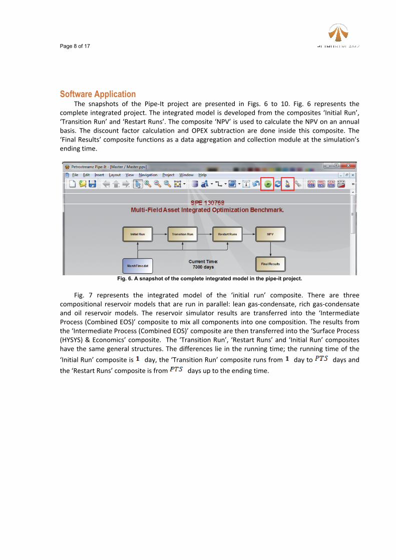
Software Application

The snapshots of the Pipe‐It project are presented in Figs. 6 to 10. Fig. 6 represents the complete integrated project. The integrated model is developed from the composites ‘Initial Run’, ‘Transition Run’ and ‘Restart Runs’. The composite ‘NPV’ is used to calculate the NPV on an annual basis. The discount factor calculation and OPEX subtraction are done inside this composite. The ‘Final Results’ composite functions as a data aggregation and collection module at the simulation’s ending time.

Fig. 6. A snapshot of the complete integrated model in the pipe-it project.

Fig. 7 represents the integrated model of the ‘initial run’ composite. There are three

compositional reservoir models that are run in parallel: lean gas‐condensate, rich gas‐condensate and oil reservoir models. The reservoir simulator results are transferred into the ‘Intermediate Process (Combined EOS)’ composite to mix all components into one composition. The results from the ‘Intermediate Process (Combined EOS)’ composite are then transferred into the ‘Surface Process (HYSYS) & Economics’ composite. The ‘Transition Run’, ‘Restart Runs’ and ‘Initial Run’ composites have the same general structures. The differences lie in the running time; the running time of the

‘Initial Run’ composite is day, the ‘Transition Run’ composite runs from day to days and

the ‘Restart Runs’ composite is from days up to the ending time.

of 17

Fig. 7. A snapshot of the ‘Initial Run’ composite.

Fig. 8 represents simulation of the ‘Lean GC Reservoir (Initial – SENSOR RUN)’ composite. The

SENSOR and STREAMS software were run inside this composite. The rich gas‐condensate and oil reservoirs also have the same composite structure. Fig. 9 shows the simulation of the ‘Intermediate Process (Combined EOS)’ composite. Fig. 10 represents the simulation of the ‘Surface Process (HYSYS) & Economics’ composite. The process starts by averaging the results of the ‘Intermediate Process (Combined EOS)’ composite. The results of the ‘Averaging’ composite are used as input data for the ‘HYSYS (RUN)’ composite.

Fig. 8. A snapshot of the ‘Lean GC Reservoir (Initial – SENSOR RUN)’ composite.

of 17

Fig. 9. A snapshot of the ‘Intermediate Process composite’.

The ‘Injection Rate Correction’ composite in Fig. 10 sums the amounts of gas and water injected

into the oil reservoir. If the available gas from the surface calculation is less than the injected gas, then the additional gas is purchased and this becomes an additional cost. On the contrary, if the available gas is greater than the injected gas, then the rest will be sold and hence generate added revenue. Inside this composite, the amount of injected gas and available gas for the gas‐condensate reservoirs are also checked. The ‘Economic Calculation’ composite calculates revenue as a function of PTS. The ‘Data Recording’ composite records the data during the simulation. In the ‘Gas Reinjection’ composite, the gas injection compositions are updated based on the results of the actual surface‐process calculation. The ‘THP‐Check’ composite checks the THP for each production well and compares it with the manifold pressure from the surface calculation. If the manifold pressure is greater than the THP, the minimum THP is adjusted to the manifold pressure.

The optimization run is controlled through a file with extension the “.ppo” (Pipe‐It Optimization). An example of an optimization file is shown in Fig. 11. The optimization solver is Reflection (based on the Nelder and Mead optimization method). The variables in yellow represent constraints, those in green represent auxiliaries, those in pink represent the objective function and those in blue represent the decision variables. The decision and constraint variables are updated before model execution but the auxiliary variables are updated after model execution. The variables are linked to numbers inside files.

Fig. 10. A snapshot of the ‘Surface Process (HYSYS) & Economics’ composite.

of 17

Fig. 11. A snapshot of an optimization file.

Base Case Simulation and Sensitivity Analysis

Base case data are shown in Table 5. The total simulation time is years and injection is

active during the first years. The simulation scenario starts with injection for years, followed by depletion of the gas‐condensate reservoirs, and water injection for the oil reservoir. The base case WAG scenario is based on scenario 2, SPE 5 Comparative solution project [Killough and Kossack,

1987]. The gas injection rate is m3/D (20000 Mcf/D), the water injection rate, m3/D

( bbl/D) and the change from water to gas injection and vice verse occurs every

days1. For the oil reservoir there are two active constraints, a gas oil ratio constraint ( Sm3/m3

or Mcf/STB) and a watercut constraint ( ). A well will shut in if it reaches one of these constraints, and re‐opened one year later. It may be noted that the water supplied for the water injection comes from an external source; hence, it is not directly linked to the process facility.

Table 5. Base-case parameters.

Value

0.4

0.3

0.6

0.5

‐30

10

3650

365

7300

Discount Factor (%)

Injection Time (days)

Project Time Step (days)

Total Simulation Time (days)

Variable

Sales Gas fraction

Fuel Gas fraction

Gas‐Condensate Reinjection fraction

Lean Reinjection fraction

DPC Temperature (C)

1 The SENSOR WAG logic specifies injection rates and cumulative slug volume per cycle.

of 17

‐1.00E+10

‐7.50E+09

‐5.00E+09

‐2.50E+09

0.00E+00

2.50E+09

5.00E+09

7.50E+09

1.00E+10

1.00E+06

2.00E+06

3.00E+06

4.00E+06

5.00E+06

6.00E+06

7.00E+06

8.00E+06

9.00E+06

0 1000 2000 3000 4000 5000 6000 7000 8000

Cumulative

NPV (USD

)

Revenue (U

SD)

Time (Days)

PTS = 1095 Days

PTS = 365 Days

PTS = 30 Days

MaximumNPV

Fig. 12. Revenues and NPVs for different PTS using base-case parameters in Table 5.

0

1500

3000

4500

6000

7500

9000

10500

0.00E+00

5.00E+05

1.00E+06

1.50E+06

2.00E+06

2.50E+06

3.00E+06

3.50E+06

0 1000 2000 3000 4000 5000 6000 7000 8000

NGL and Condensate (SM

3/D

)

Sales Gas (SM

3/D

)

Time (days)

Sales Gas ‐ PTS 30D Sales Gas ‐ PTS 365D NGL ‐ PTS 30D

NGL ‐ PTS 365D Condensate ‐ PTS 30D Condensate ‐ PTS 365D

Fig. 13. Field products in volume units for different PTS values.

The annual NPV performance for the base case is presented in Fig. 12. This figure shows that for

the base‐case parameters, the field should be operated for years, from an economic point of

view. A varying PTS does not change (annual‐based) NPV significantly. NPV calculations in Fig.

of 17

12 are made with Eq. 4 and days. Figure 13 shows the sales gas, NGL, and condensate performances for the base‐case parameters. This figure shows that sales gas increased after the end of the injection scenario, but later showed a downturn.

The base case simulator and scenario were analyzed by perturbing several key parameters, i.e., the key decision variables in this benchmark case, including: (i) The dew point temperature controlling NGL extraction, (ii) The gas sales fraction (fraction sales gas of total produced gas, TEE1 top‐right in Fig. 3), (iii) The gas‐condensate reinjection fraction (fraction of reinjected gas into gas condensate reservoirs, TEE3 top‐right in Fig. 3) and (iv) The lean reinjection fraction (fraction reinjected gas into lean reservoir, TEE4 top‐right in Fig. 3). For the reservoir aspect, it is possible to optimize the WAG period and the amount of gas and water injection rates. All other decision variables were held constant during a simulation run. Figure 14 (a) is an example of single parameter analysis for an optimization variable and Fig. 14 (b) shows surface parameter analysis when two parameters are changed simultaneously. The parameter sensitivity results are summarized in Table 6. The highest NPV increment (9%) was obtained by changing the sales gas fraction and DPC temperature. Figures 10 (a) and (b) show the day at which a maximum NPV is reached. It can be concluded from the study that nonlinear effects are significant and thus local optima are present in this problem. The simulation was run on a 2.67 GHz, 2 Quad core CPU with 8 GB of RAM. Applying PTS of 365 days (1 year) and the run time was about ~336 seconds.

3650

3650

3650

3650 4015

365

01540154015

5.80E+9

5.85E+9

5.90E+9

5.95E+9

6.00E+9

6.05E+9

6.10E+9

0 50 100 150 350 400

Maximum NPV (U

SD)

Delta WA

0 3650

36503650

4015

4

200 250 300

G Cycle (days)

Base Case

0.1

0.3

0.5

0.7

0.9

5.4E+9

5.6E+9

5.8E+9

6.0E+9

6.2E+9

6.4E+9

6.6E+9

6.8E+9

‐55 ‐50 ‐45 ‐40 ‐35 ‐30 ‐25 ‐20 ‐15 ‐10

Maximum NPV (U

SD)

DPC Temperature (C)

3650Base Case

(a). Single parameter analysis for the WAG cycle time. This figure indicates that the best scenario for the oil reservoir is implementing Simultaneous WAG (SWAG).

(b). Surface parameter analysis for DPC temperature and sales gas fraction.

The maximum NPV is obtained when

and oC.

Fig 14. Sensitivity parameter analysis for single and surface parameters.

Table 6. Sensitivity parameter results. The optimal value and corresponding NPV are shown for each of the single parameter and two parameter sensitivity analyses, respectively.

of 17

Case Optimal Value NPV (USD) Base Case ValueNPV ‐ Base

Case (USD)

Increment

(%)

DPC Temperature ‐55 C 6.43E+09 ‐30 C 6.03E+09 6.22

Sales Gas Fraction 0.3 6.17E+09 0.4 6.03E+09 2.23

Gas‐Condensate

Reinjection Fraction0.1 6.28E+09 0.6 6.03E+09 3.92

Lean GC Reinjection

Fraction0.6 6.23E+09 0.5 6.03E+09 3.21

WAG Cycle Period 30 days 6.09E+09 91.25 days 6.03E+09 0.90

qgi and qwi for oil

reservoir

qgi = 849505.5 m3/D

qwi = 5564.5 m3/D6.52E+09

qgi = 566337 m3/D

qwi = 7154.4 m3/D6.03E+09 7.56

GC Inj Fract and Lean

Inj Frac

fRgc = 0.1 and fRL =

0.66.43E+09

fRgc = 0.6 and fRL =

0.56.03E+09 6.22

Sales Gas Frac and

DPC Temp

fsg = 0.5 and T DPC = ‐

55 C6.63E+09

fsg = 0.4 and T DPC = ‐

30 C6.03E+09 9.08

Optimization The Nelder‐Mead Simplex Reflection method constrained handler is applied for two different

optimization scenarios to maximize the NPV. The decision variables for the first scenario are DPC temperature, sales gas fraction, gas‐condensate reinjection fraction and lean gas‐condensate reinjection fraction. The decision variables for the second scenario are sales gas fraction, DPC temperature, gas injection rate and water injection rate for WAG scenario and WAG period. The decision variables were defined based on the results from sensitivity study. The first scenario focused on the surface facilities parameter optimization, while the second scenario is the combination of surface facilities and reservoir parameters. These optimization models can be described as the following:

Scenario 1

with the following constraints on the decision variables

Scenario 2

with the following constraints on the decision variables

The base‐case parameters in Table 5 were used as the initial value for the optimization. The

optimization results for scenario 1 are: and

of 17

the optimization results for scenario 2 are:

. The comparison between base case and the optimization results is presented in Table 7 and early

shows the potential of optimization since NPV has increased ~ % and ~ %, respectively. Scenario

1 required iterations to converge to the optimum solution, while scenario 2 took iterations. The base case CPU run time for optimization scenario 1 was ~2 hours and it was ~7 hours for Scenario 2.

Table 7. Comparison of base-case and optimization results.

Parameter Base Case Scenario cenario 2

Cumulative sales gas (m3) 1.05E+10 E+10 1.11E+10

Cumulative NGL (m3) 5.52E+06 E+06 7.45E+06

Cumulative Condensate (m3) 3.59E+07 E+07 4.66E+07

NPV (USD) 6.03E+09 .61E+09 7.82E+09

Number of iterations 1 29 73

CPU run time (hour) 0.09 2.06 7.02

Increment from the base case ‐ 9 % ~ 23%

Op n

1 S

timizatio

1.12

6.75

3.58

6

~

Conclusion The presented I‐OPT model is suitable for assessing the potential of integrated optimization

since the upstream and downstream parts of the model are tightly coupled. Optimization has a clear potential because the multi‐variable scenarios considered in this paper reveal an NPV increase of

% ‐ % compared to the base case gas injection scenario. Figure 15 shows that the magnitude of total NPV error is more‐or‐less constant for a given

, in both base‐case and the optimization cases in Scenarios 1 and 2. We therefore concluded

that the surface of maximum NPV is rather insensitive to , and thus compromised using a

of 1 year for the optimizations. Once an optimal case is located, the I‐OPT project is rerun with a smaller project time step (e.g. 1 month) to obtain a more‐accurate (“true”) value of the maximum NPV.

Figure 15 also shows that there was only a small gain to be made in terms of run time if the project time step is increased beyond 1 year. However, a shorter project time step increases the computational cost substantially. The NPV is shown for the varying project time steps. The base case NPV curve is equal to Fig. 4(a). One might argue for the selection of different project time steps depending on the run time and hardware resources available. (Juell et al., 2010) improved the NPV result for a given project time step by introducing intermediate “division” project time steps whereby reservoir results were fed to the (fast and approximate) proxy surface process model

of 17

without feedback. This approach was not used in our benchmark because the surface process is a real and more complex model therefore CPU time was much higher.

4.0E+9

4.5E+9

5.0E+9

5.5E+9

6.0E+9

6.5E+9

7.0E+9

7.5E+9

8.0E+9

0

5

10

15

20

25

30

35

40

0 200 400 600 800 1000 1200 1400

Maxim

um NPV (USD

)

CPU tim

e (relative

to the base case tim

e)

Project time step (days)

Scenario 2 Optimum

Scenario 1Optimum

Base Case

Fig. 15 NPV for different project time steps.

Nomenclature = Discount factor

= Total project time step

= Mass of CO2 removal, MT/day

= Power consumption, KW/day

sales gas fraction

reinjected gas fraction,

gas‐condensate reinjection fraction

oil reinjection fraction,

lean gas‐condensate reinjection fraction

rich gas‐condensate reinjection fraction,

= Condensate production rate, m3/day

= Gas production rate, m3/day

= NGL production rate, m3/day

= Surface water injection rate, m3/day

= Surface water production rate, m3/day

= Condensate price, USD/ m3

= NGL price, USD/ m3

= Power cost, USD/kWh

of 17

= Water injection and production cost, USD/ m3

= CO2 removal cost, USD/MT

= Dew Point Controller temperature, oC

= Project time step, days

= Project time step equal to 365 days

WAG cycle time, days

Acknowledgements

We acknowledge our collegues Mohammad Faizul Hoda from PERA and Aleksander Juell from Norwegian University of Science and Technology (NTNU). We are grateful for the assistance from Prof. Michael Golan at NTNU, Robert Hubbard from John M. Campbell&Co and Ken Starling from Starling & Associates, for helping with the surface process development. We also acknowledge financial support by the Center for Integrated Operations in the Petroleum Industry at NTNU.

References Juell, A., Whitson, C.H., and Hoda, M.F. 2009. Model Based Integration and Optimization Gas Cycling Benchmark. Paper SPE 121252. SPE Journal, September 2010. Killough, J.E., and Kossack, C.A. 1987. Paper SPE 16000. Fifth SPE Comparative Solution Project: Evaluation of Miscible flood Simulators.

Pipe-It Case Study Multi Field Asset Integrated...

Documents

Transcript of Pipe-It Case Study Multi Field Asset Integrated...