MODELING STRENGTH AND STIFFNESS OF INTENSIVELY MANAGED LOBLOLLY

PINE PLANTATIONS IN THE ATLANTIC COASTAL PLAIN OF GEORGIA

by

MARK ALEXANDER BUTLER

(Under the Direction of Joseph Dahlen)

ABSTRACT

Strength and stiffness, or modulus of rupture (MOR) and modulus of elasticity (MOE),

are critical properties in determining how well lumber perform in structural applications.

Intensively grown, plantation loblolly pine (Pinus taeda) has lower MOR and MOE than that of

slower grown trees when harvested with similar dimensions, based on recent research by the

Southern Pine Inspection Bureau (SPIB). A total of 93 trees were harvested from the Atlantic

Coastal Plain of Georgia, and were processed at a lumber mill into nominal 2 inch wide material

(ex. 2×4). After nondestructively and destructively sampling the lumber from the trees, a model

predicting MOE was generated for several scenarios and stages of the harvesting and milling

process. The most basic model predicts the MOE of each log from its acoustic velocity

measurement (R2 = 0.52). Knowing certain tree or log characteristics, such as diameter at certain

points up the bole, age, and height can increase the ability to predict MOE and MOR. A model

that predicts MOE from log position, specific gravity, and several diameter measurements, as

well as the acoustic velocity of each log had an R2 of 0.70. This relationship suggests that lumber

mills could use acoustic velocity as a MOE predictor to sort higher quality logs.

INDEX WORDS: Modulus of rupture, Modulus of elasticity, Loblolly pine, Intensive

management, Static bending

MODELING STRENGTH AND STIFFNESS OF INTENSIVELY MANAGED LOBLOLLY

PINE PLANTATIONS IN THE ATLANTIC COASTAL PLAIN OF GEORGIA

by

MARK ALEXANDER BUTLER

BSFR, University of Georgia, 2012

A Thesis Submitted to the Graduate Faculty of the University of Georgia in Partial Fulfillment of

the Requirements for the Degree

MASTER OF SCIENCE

ATHENS, GEORGIA

2015

© 2015

Mark Alexander Butler

All Rights Reserved

MODELING STRENGTH AND STIFFNESS OF INTENSIVELY MANAGED LOBLOLLY

PINE PLANTATIONS IN THE ATLANTIC COASTAL PLAIN OF GEORGIA

by

MARK ALEXANDER BUTLER

Major Professor: Joseph Dahlen

Committee: Richard Daniels

Michael Kane

Electronic Version Approved:

Suzanne Barbour

Dean of the Graduate School

The University of Georgia

August 2015

iv

DEDICATION

I dedicate this thesis to the people in my life, without whom this endeavor would not

have been possible. I would like to thank my father and mother, Mark and Melanie Butler, for

instilling in me a great work ethic and a passion for achieving my goals. I would also like to

thank my committee for their dedication and guidance towards the completion of this thesis.

Thank you Dr. Dahlen, your encouragement and foresight allowed me to pursue this project,

thank you Dr. Daniels for your passion for students and seeing them succeed, thank you Dr.

Kane for your dedication and commitment to research at Warnell. I would also like to thank my

loving wife, Ashley Butler, who has encouraged me to stay on task and to strive for more. Lastly,

I want to thank God, through which all things are possible.

v

ACKNOWLEDGEMENTS

I would like to thank Plum Creek Timber Company, without whose assistance with land,

time, and funding, this thesis would not have been possible. I would also like to thank Varn

Wood Products for the use of their lumber yard, mill facility, and their assistance in processing

our raw logs.

I would also like thank The Wood Quality Consortium for funding and support of this

project. Individually I would like to acknowledge the help and support of Edward Andrews from

the U.S. Department of Agriculture Forest Service, for his assistance in harvesting the sample

trees. I would like to acknowledge Bryan Simmons and Thomas Bennett for their assistance with

setting up and measuring sample plots, harvesting trees, and for helping to prepare and test

lumber. I would like to thank Sam Varn for his help in preparing logs to go through the milling

process. I would also like to acknowledge Dr. Finto Antony for his work in statistics,

experimental design, and his assistance in the field work portion of this project.

vi

TABLE OF CONTENTS

Page

ACKNOWLEDGEMENTS .............................................................................................................v

LIST OF TABLES ....................................................................................................................... viii

LIST OF FIGURES ....................................................................................................................... ix

CHAPTER

1 INTRODUCTION ........................................................................................................1

Purpose of the Study ...............................................................................................1

How the Study is Original.......................................................................................1

Expected Results .....................................................................................................2

2 LITERATURE REVIEW .............................................................................................3

History of Pine Plantation Management in the Southeastern U.S ..........................3

Intensive Forest Management Linked to Wood Quality .........................................4

Southern Pine Inspection Bureau, Lumber Grading and Inspection .......................5

Nondestructive Testing of Wood ............................................................................7

Standing Tree Approach .........................................................................................7

Log Based Approach...............................................................................................8

Nondestructive Evaluation of Lumber ....................................................................9

3 MATERIALS AND METHODS ................................................................................10

Stand Selection......................................................................................................10

Inventory ...............................................................................................................10

vii

Tree Felling and Nondestructive Testing ..............................................................11

Milling and Processing .........................................................................................11

Nondestructive Physical Tests for Lumber ...........................................................12

Static Bending .......................................................................................................14

Lumber Adjustments .............................................................................................16

Statistical Analysis ................................................................................................18

4 RESULTS AND DISCUSSION .................................................................................20

Longitudinal Wave Stress .....................................................................................20

Grade Distribution ................................................................................................22

Mechanical Properties of Lumber .........................................................................26

Predicting MOE with Various NDE Tests ............................................................29

Modeling MOE from Lumber NDE .....................................................................30

5 CONCLUSIONS.........................................................................................................35

REFERENCES ..............................................................................................................................37

viii

LIST OF TABLES

Page

Table 3.1: Stand inventory and sample tree data. .. .......................................................................11

Table 4.1: Average acoustic velocity measurements (meters/second) from felled trees and

individual logs. ...............................................................................................................................20

Table 4.2: Breakdown of grade distribution of processed lumber by log position and stand........24

Table 4.3: Average grade produced by stand. ................................................................................25

Table 4.4: Average grade produced by log position. .....................................................................26

Table 4.5: Average MOE15, aggregated by log, for each stand. ....................................................26

Table 4.6: Mechanical properties of lumber by log position and grade. .......................................27

Table 4.7: Prediction of MOE15 using nondestructive lumber evaluation .....................................29

Table 4.8: R2 values and residual standard errors for eight predictions of MOE15. ......................33

ix

LIST OF FIGURES

Page

Figure 4.1: Log acoustic velocity based on log position within the stem (min, max, 1Q, 3Q, and

median). .........................................................................................................................................21

Figure 4.2: Log acoustic velocity by lumber grade (min, max, 1Q, 3Q, and median)….. ............22

Figure 4.3: Interaction plot for MOR15 between log position and grade. ......................................28

Figure 4.4: Interaction plot for CMOR15 between log position and grade. ...................................28

Figure 4.5: Interaction plot for MOE15 between log position and grade. ......................................29

Figure 4.6: Relationship between log acoustic velocity and aggregate MOE15 by log. ................31

Figure 4.7: Relationship between acoustic velocity and aggregate MOE15 by tree .......................32

1

CHAPTER 1

INTRODUCTION

Purpose of the Study

The purpose of this study is to create a model for loblolly pine that predicts lumber

stiffness and strength with characteristics and nondestructive tests conducted on whole trees,

individual logs, and individual lumber pieces. Lumber strength (modulus of rupture (MOR)) and

stiffness (modulus of elasticity (MOE)) are critical properties because of their importance in

construction and other structural uses. In recent years as forest management has intensified,

concern over wood quality has increased, especially in the southeastern United States where tree

growth rates have increased substantially. This tree growth increase can have a negative impact

on wood quality. By harvesting mature trees which were grown intensively, certain properties of

the tree can be measured while it is standing, after it is cut, and after it has been processed into

lumber at a lumber mill. Nondestructive testing performed during these phases can be used to

predict MOE and MOR. It is the belief of the author that findings of this study will present a

clearer picture of how intensive management is affecting wood quality of southern pine.

How the Study is Original

The present study deals with loblolly pine (Pinus taeda) trees, ages 24-33, (site index

(SI25) from 25 m to 27 m), grown in the Atlantic Coastal Plain of southeastern Georgia. These

trees were all grown under intensive management and the stands have reached maturity. The

author marked and recorded each tree so that it could be individually tracked during harvest and

through the lumber milling process. Each piece of lumber can be tied back to the tree from which

2

it came. Also lumber was then tested independently to assure accuracy of tests and records. The

lumber was tested using a universal testing machine setup in static bending to measure MOR and

MOE. The author then used the measured properties and nondestructive test results to create a

model which predicts MOR and MOE. It is commonly believed that intensively managed

loblolly pine has reduced mechanical wood properties due to an increase in juvenile corewood

from intensive management (Clark et al. 2008). Few studies have addressed the exact impact of

intensive management on the mechanical properties of lumber.

Expected Results

The author hypothesizes that the nondestructive tests, as well as measured tree, log, and

lumber characteristics can be used to successfully create a model that predicts MOE and MOR.

The author also hypothesizes that conclusions from this study can be drawn to broadly discuss

the impact of intensive forest management on wood quality. The author hopes the results of this

study will be impactful and meaningful for the forest products industry, as well as forest

managers across the Southeast. Knowing how accurately MOR and MOE can be predicted from

nondestructive testing could potentially add these tests as a normal step of the harvesting or

milling process which would give a better picture of actual lumber strength and stiffness before it

is used in a structural or construction project.

3

CHAPTER 2

LITERATURE REVIEW

History of Plantation Management in the Southeast

In the 1950s abandoned agriculture land dominated the southeastern United States

landscape. There were around 2 million acres of planted pines (Pinus spp.), but by the end of the

20th

century there were over 30 million acres of pine plantations in the South (Wear and Greis

2002). With this increase in pine plantations came an upturn in interest in intensive management.

Intensive forest management (IFM) has been a key tool in managing pine plantations in

southeastern United States timberlands since the early 1950s (Stanturf et al. 2003). Commercial

pine stands in this region are dominated primarily by loblolly pine (Pinus taeda) and slash pine

(Pinus elliottii). Over the past 60 years, the development of IFM has transitioned forestry in the

South from naturally grown stands to a system of plantation dominated management.

IFM practices such as intensive site preparation, fertilization, competition control, and

density control help speed up tree growth in pine plantations (Jokela et al. 2010). Significant

advancements have also been made using genetically improved seedlings, and increasingly in the

future, clones will be deployed in the field. Bettinger et al. (2009) states that tree breeding

programs are a key component of plantation forestry with regard to increasing tree growth.

Faster growth rates increase wood volume harvested, as well as shorten rotation lengths.

However, rapid growth rates also increase the percentage of juvenile corewood, thus reducing

lumber strength, value, and quality due to reduced stiffness or modulus of elasticity (MOE)

(Larson et al. 2001). MOE is a measure of the resistance of the wood to deformation due to

4

applied stress (Roth et al. 2007). Modulus of rupture (MOR) is the amount of stress at which a

substance breaks. Mechanical properties are known to decrease with a rise in growth rates and

percentage of corewood harvested (Antony et al. 2011).

Intensive Forest Management Linked to Wood Quality

Many studies have correlated IFM practices with higher growth rates and higher

production yields in southern pine plantations. For example, thinning pine stands has been shown

to increase growth rates and production of pine plantations (Baldwin et al. 2000). Fertilization

and weed control have been shown to speed up stand growth and increase average tree size

(Zhao et al. 2011). Site preparation that improves soil conditions and controls competing

vegetation can result in increased seedling survival and growth (Löf et al. 2012).

Some of the outcomes of IFM can be negative as well. With increased growth rates of

pine plantations in the early years of a rotation comes an increase in the juvenile wood to mature

wood ratio (Roth et al. 2007). Juvenile wood is less desirable because it has lower MOE levels.

MOE and MOR can be explained by a variation in microfibril angle (MFA), wood density,

knots, and grain angle (Cramer et al. 2005). MFA refers to the angle of the microfibrils in

relation to the vertical cells in the secondary cell wall of woody plants (Kretschmann et al. 1998).

Juvenile wood has a higher MFA than mature wood. Studies have linked IFM practices with

reduced wood quality due to high juvenile wood content. In a radiata pine (Pinus radiata)

plantation study in New Zealand, understory vegetation was controlled for two years which

resulted in a 93% reduction in MOE (Watt et al. 2005). Fertilization resulted in lower densities,

higher MFA, and slightly less stiffness in Pinus radiata in Australia (Downes et al. 2002). Early

thinning can also result in wood with inferior strength properties (Wang et al. 2001).

5

A significant portion of lumber from loblolly pine plantations (ages 25, 30, and 35) in

West Central Alabama did not meet design values for strength and stiffness for the assigned

visual grade (Biblis et al. 1993). The study found that the older stands had a higher proportion of

lumber that reached the strength and stiffness design values. A second study on the same trees

found that planting density is also a significant factor in determining lumber quality whereby

increases in planting density results in an increase in the percentage of lumber that met the

strength and stiffness design values (Biblis et al. 1995). Fast grown loblolly pine from

intensively managed stands has resulted in an expectation of less material meeting visually-

graded design values. Such observations suggest that several commonly used IFM practices can

decrease desirable properties of wood, such as high MOR and MOE.

Southern Pine Inspection Bureau, Lumber Grading and Inspection

Lumber is visually or mechanically inspected before leaving a mill. Most lumber in the

United States is visually inspected according to ASTM D245 (2006). A visual inspection results

in a lumber grade, and each grade has an associated strength and stiffness standard that each

lumber should meet.

Because of a decrease in MOE and MOR from much of the plantation grown pines, IFM

practices have been linked to the production of wood that does not meet Southern Pine

Inspection Bureau (SPIB) design value requirements. For the past thirty years lumber standards

were based off of full scale lumber testing conducted in the 1980s (Green and Evans1988). In

June 2012, the SPIB implemented new design values that lowered the visually graded strength

and stiffness levels for many southern pine lumber products (Southern Forest Products

Association 2012). These lowered strength levels are a direct result of the predicted reduction in

MOR and MOE. Reducing strength characteristics of trees to accommodate for high volume

6

production has professionals within the forestry and wood products industry worried about the

future of southern pine lumber quality and value.

The SPIB, the inspection agency for southern pine lumber, indicated that all grades of

visually inspected lumber two to four inches thick, and two inches or wider should have their

design values lowered. In the initial study that first sparked the design value discussion, the SPIB

found that 10% of lumber pieces that were visually inspected and graded had lower strength

levels than the minimum strength standards for its particular visual grade (Southern Forest

Products Association 2011). In 2011, The Southern Pine Design Value Forum (SPDVF) asked

the SPIB to reconsider their recommendations based on the fact that their extrapolation of the

testing results to other sizes and grades besides the No. 2 2×4 was not appropriate per ASTM

D1990 (2014). The SPDVF used a Mississippi State University study as evidence, which found

that only 6% of lumber pieces failed to meet the required strength levels in the No. 2 2×4 grade

and size (Dahlen et al. 2012). Additional testing conducted and presented in the wide dimension

material (2×6 to 2×12 size and No. 2 grade) showed that the testing results generally improve as

size increases (Dahlen et al. 2014). This additional evidence generally showed that extrapolation

of the testing results beyond the 2×4 size was not appropriate. The main goal of the SPDVF was

to delay the ALSC (American Lumber Standards Committee) from implementing the new

standards until more testing could be completed. The design values for southern yellow pine

were revised by the ALSC in 2013. Most sizes and designs were affected by the reduction of the

standards (Southern Forest Products Association 2013) however the reduction was not as severe

as originally thought and some design values did not change.

Further advancements and intensification in forest management are expected. However,

advancements might be curtailed due to the lowering of southern pine strength and stiffness

7

standards for visually inspected wood (Jokela et al. 2010). Further declines in MOE and MOR

would degrade the quality, value, and use of southern pine lumber resulting in a potential

negative impact on southeastern U.S. pine markets and prices (Roth et al. 2007). If current IFM

practices produce lower quality wood, fear of substantial reduction in southern pine quality and

value may encourage changes in how pine plantations are managed.

Nondestructive Testing of Wood

Nondestructive testing can be an extremely helpful science for testing different physical

and mechanical properties of a material without destroying its end use capabilities (Pellerin and

Ross 2002). Nondestructive evaluation (NDE) methods can range from visual inspection of a

piece to chemical or mechanical testing. Furthermore NDE methods can be utilized for many

different types of materials and at various stages of the wood manufacturing process. NDE is

often an effective way to sort logs and lumber by stiffness (Carter et al 2006).

Standing Tree Approach

One way to measure acoustic velocity in standing trees is by the time-of-flight approach

(Grabianowski et al. 2006). An acoustic wave transmission pin (Tx) and a receiver pin (Rx) are

tapped into the tree approximately 1 meter apart. The pins are usually vertically aligned.

Acoustic waves will be measured by gently striking the Tx pin and measuring the time it took to

get to the Rx pin. The velocity will be calculated by

V = l/t

Where V is the velocity of the wave, l is the distance between the pins, and t is the time it took

for the wave to travel between the pins. The relationship between MOE and velocity is:

MOE = pVtf2

8

Where p is the density of the tree (green density) and V is the velocity as measured by time-of-

flight. Typically green density has been assumed to be relatively constant (Lasserree et al. 2009)

although this assumption is likely not accurate but acceptable given the effort needed to

accurately measure density (Wang 2013). Mora et al. (2009) state that the standing tree method

overstates static MOE values and cannot predict “true” MOE of the tree, but that it can be used

as a ranking tool for breeding purposes.

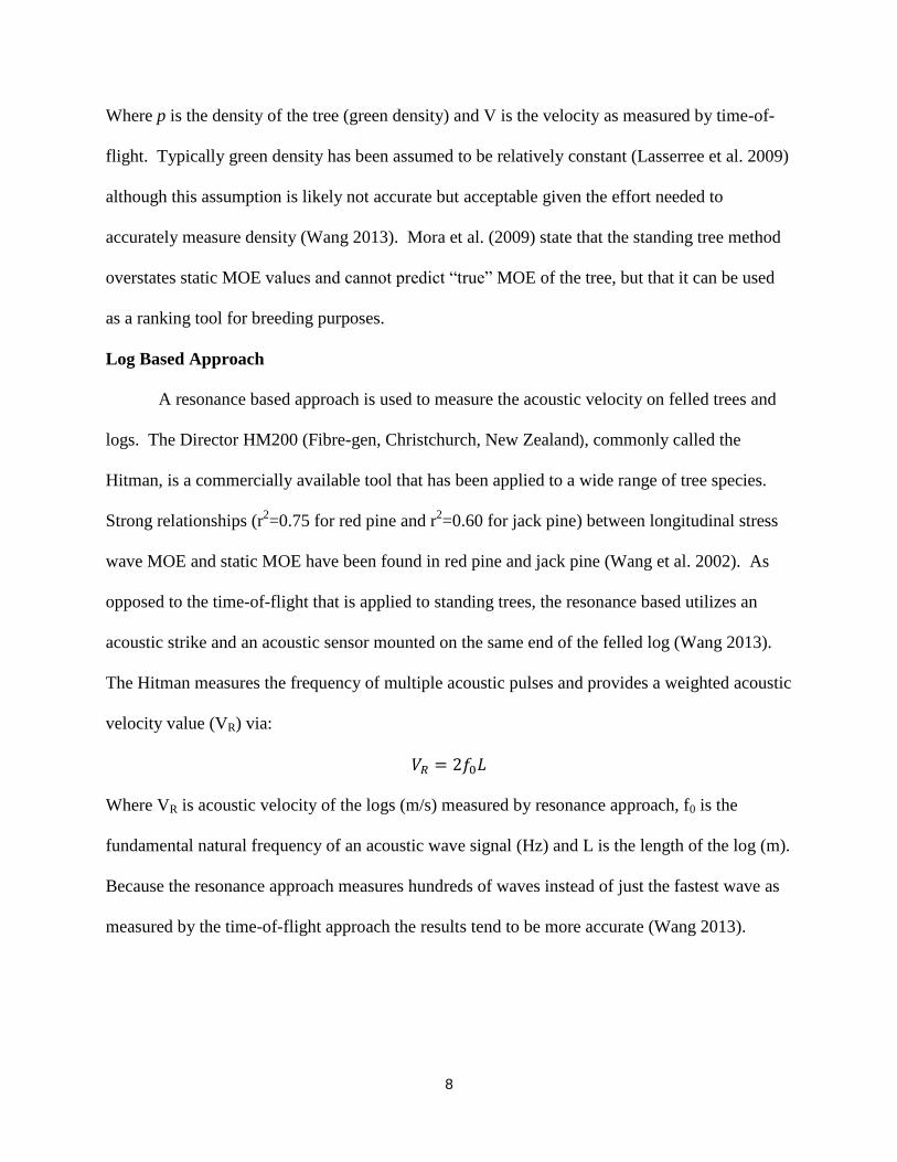
Log Based Approach

A resonance based approach is used to measure the acoustic velocity on felled trees and

logs. The Director HM200 (Fibre-gen, Christchurch, New Zealand), commonly called the

Hitman, is a commercially available tool that has been applied to a wide range of tree species.

Strong relationships (r2=0.75 for red pine and r

2=0.60 for jack pine) between longitudinal stress

wave MOE and static MOE have been found in red pine and jack pine (Wang et al. 2002). As

opposed to the time-of-flight that is applied to standing trees, the resonance based utilizes an

acoustic strike and an acoustic sensor mounted on the same end of the felled log (Wang 2013).

The Hitman measures the frequency of multiple acoustic pulses and provides a weighted acoustic

velocity value (VR) via:

Where VR is acoustic velocity of the logs (m/s) measured by resonance approach, f0 is the

fundamental natural frequency of an acoustic wave signal (Hz) and L is the length of the log (m).

Because the resonance approach measures hundreds of waves instead of just the fastest wave as

measured by the time-of-flight approach the results tend to be more accurate (Wang 2013).

9

Nondestructive Evaluation of Lumber

Lumber has a long history of NDE through the visual grading process. The most common

reasons lumber is degraded are for knots (size, location, and number), slope of grain, wane, and

other physical deformities. Typical grades include Select Structural, No. 1, No. 2, No. 3 and Stud

grades with the higher grades having higher stiffness and strength.

Acoustic velocity can be used to grade lumber using the resonance approach for felled

logs (Hitman). Additionally the resonance can be measured by using different resonance

approaches where an acoustic wave is made on one end of the lumber and the resonance is

measured on the other end using a microphone. The microphone oscilloscope measures the

frequency from the end of the lumber which is converted to the speed of the sound waves.

The transverse vibration method is also used to measure dynamic MOE for lumber. This

method uses a tool called the E-computer (Metriguard), and involves resting each piece of

lumber on fixed points with equal overhang on both sides. A downward tap on the wide face of

the lumber allows the E-computer to measure the stiffness of the lumber by the frequency of

oscillations. It is essential that lumber length and the span between the resting points remain

constant for same sized lumber. Dynamic MOE is then calculated by:

Where fn is the undamped natural frequency, W is the weight, L is the span, K is the adjustment

constant, b is the width of the specimen, and h is the thickness.

This method has been used widely in research. Ross et al. (1991) found an r-value of 0.99 when

comparing dynamic MOE from the E-computer and static bending MOE.

10

CHAPTER 3

MATERIALS AND METHODS

Stand Selection

This study is focused on loblolly pine which is one of the major species for the southern

pine group. The area of focus is the Atlantic Coastal Plain in southeast Georgia. This area has

some of the highest growth rates in the country as well as a history of plantation forestry

management. The timber stands that were selected are managed by Plum Creek Timber

Company. Five stands were chosen for the study. The stands vary in age from 24 to 33 years old.

The stands were located in Glynn, Camden, and Wayne counties. A general silvicultural and

management history is known for each stand. They have all been thinned at least once while

some have been thinned twice. The stands have had varied degrees of management including site

preparation, fertilization, competition control for woody and herbaceous competitors, and were

planted with quality seedlings at approximately 1,550 trees per hectare.

Inventory

A total stand inventory was known for each stand, while a more specific plot inventory

was taken around the sample trees. Plot locations were selected at random for each stand. At

each plot location a specific number of trees were selected from 2.5 cm diameter classes between

21.6 cm and 36.8 cm, based on an average size distribution across the entire stand. The trees

were selected by using a proportion of lumber feet per acre from the entire stand. There was

more focus on larger diameter trees. Three stands had 21 trees, one stand had 20 trees, and one

stand had 10 trees selected for harvest. At each plot location trees per hectare, basal area, tree

11

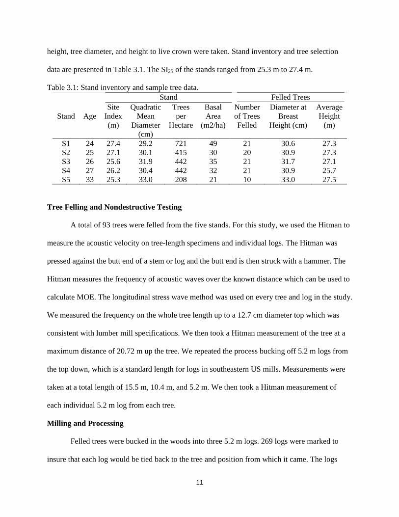
height, tree diameter, and height to live crown were taken. Stand inventory and tree selection

data are presented in Table 3.1. The SI25 of the stands ranged from 25.3 m to 27.4 m.

Table 3.1: Stand inventory and sample tree data.

Stand Felled Trees

Stand

Age

Site

Index

(m)

Quadratic

Mean

Diameter

(cm)

Trees

per

Hectare

Basal

Area

(m2/ha)

Number

of Trees

Felled

Diameter at

Breast

Height (cm)

Average

Height

(m)

S1 24 27.4 29.2 721 49 21 30.6 27.3

S2 25 27.1 30.1 415 30 20 30.9 27.3

S3 26 25.6 31.9 442 35 21 31.7 27.1

S4 27 26.2 30.4 442 32 21 30.9 25.7

S5 33 25.3 33.0 208 21 10 33.0 27.5

Tree Felling and Nondestructive Testing

A total of 93 trees were felled from the five stands. For this study, we used the Hitman to

measure the acoustic velocity on tree-length specimens and individual logs. The Hitman was

pressed against the butt end of a stem or log and the butt end is then struck with a hammer. The

Hitman measures the frequency of acoustic waves over the known distance which can be used to

calculate MOE. The longitudinal stress wave method was used on every tree and log in the study.

We measured the frequency on the whole tree length up to a 12.7 cm diameter top which was

consistent with lumber mill specifications. We then took a Hitman measurement of the tree at a

maximum distance of 20.72 m up the tree. We repeated the process bucking off 5.2 m logs from

the top down, which is a standard length for logs in southeastern US mills. Measurements were

taken at a total length of 15.5 m, 10.4 m, and 5.2 m. We then took a Hitman measurement of

each individual 5.2 m log from each tree.

Milling and Processing

Felled trees were bucked in the woods into three 5.2 m logs. 269 logs were marked to

insure that each log would be tied back to the tree and position from which it came. The logs

12

were transported to a participating lumber mill where they ran through the head rig, gang saw,

edger, and were sawn into 4.9 m lumber pieces. The logs were sawn into 2×4, 2×6, 2×8, and

2×10 lumber. The lumber was kiln-dried below 19 percent moisture content, then planed, and

given a grade by Timber Products Inspection, Inc. certified graders. The logs resulted in 841

pieces of lumber in grades No. 1, No. 2, and No. 3. There were also several grade No. 4 lumber

but these were not considered for this study due to their poor form and increased variability.

Another NDE method that was utilized in this study was visual grading of lumber. The

most common reasons lumber is degraded are for knots (size, location, and number), wane, and

other physical deformities. Graders assigned a number grade (1-4) to each lumber as they went

through the milling process, 1 being the highest quality lumber, and 4 being the most degraded.

These number grades are standard grades given to pine lumber in southeastern US mils. We used

these grades to help predict static MOE and MOR. No. 4 lumber produced was due to the

constraints of not running the lumber through the optimized trimmer and forcing nominal 2-inch

material because the focus of the study was on structural dimensional lumber.

Nondestructive Physical Tests for Lumber

After the lumber were processed and visually graded, they were transported to the wood

quality laboratory at the University of Georgia in Athens, Georgia. We took a number of

physical attributes and measurements such as size measurements, weight, moisture content, and

growth rings per inch from both ends of the lumber. We measured the average width, thickness,

and the total length for each piece of lumber. Presence or absence of pith and knots were

recorded for each lumber piece. We also used the Hitman again to measure the acoustic velocity

for each individual lumber piece. The Hitman measurements of each lumber piece were

compared to the Hitman reading from its respective log and tree. Each lumber piece was cut to

13

its testing span which included the largest defect of the lumber randomly located in the testing

span.

For each lumber piece we also conducted two additional NDE tests. The PLG (Portable

Lumber Grader) was used as a resonance test whereby a wave is initiated from one end of the

lumber with a hammer to the other end and the frequency of the pulse is measured with a

microphone. The microphone oscilloscope measures the frequency from the end of the lumber

which is converted to the speed of the sound waves. This is another test of MOE.

The final NDE method used on each lumber is a transverse vibration method that also

measures resonance. This method uses a tool called the E-computer (Metriguard), and involves

resting each lumber on fixed points with equal overhang on both sides. For our testing we set the

lumber on two static points to insure that there were approximately 2.5 cm of overhang on each

side. A downward tap on the wide face of the lumber allows the E-computer to measure the

stiffness of the lumber by the frequency of oscillations. It is essential that lumber length and the

span between the resting points remain constant for same sized lumber. This method has been

used widely in research. Ross et al. (1991) found an r-value of 0.99 when comparing dynamic

MOE from the E-computer and static bending MOE.

The benefit of NDE methods is that it allows the tester to examine physical and

mechanical properties of green wood or processed wood, without altering its end use. This is

essential to wood manufacturers who might be reluctant to conduct testing which would render

some of their product unusable. One objective of this study is to compare measures of MOE and

MOR using NDE methods with static bending to determine what relationships might exist for

intensively managed loblolly pine. This could help many of the players in the wood industry

make more accurate predictions of wood quality whether in the green form or in an end product.

14

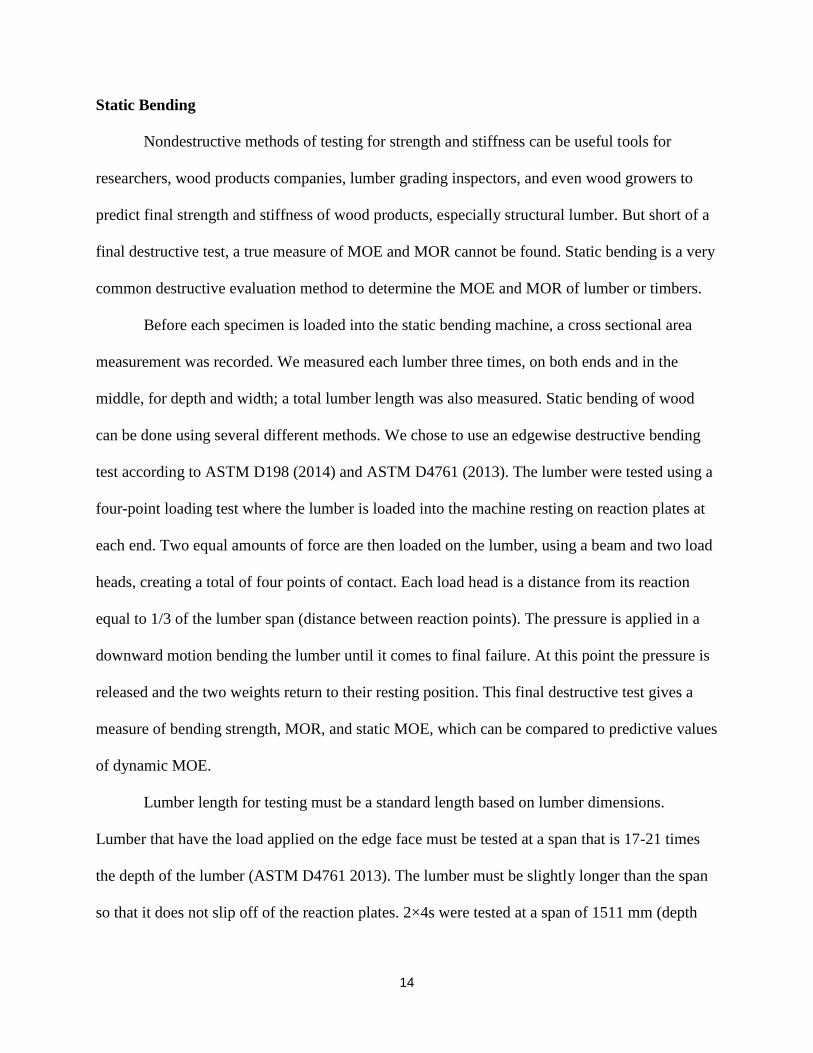
Static Bending

Nondestructive methods of testing for strength and stiffness can be useful tools for

researchers, wood products companies, lumber grading inspectors, and even wood growers to

predict final strength and stiffness of wood products, especially structural lumber. But short of a

final destructive test, a true measure of MOE and MOR cannot be found. Static bending is a very

common destructive evaluation method to determine the MOE and MOR of lumber or timbers.

Before each specimen is loaded into the static bending machine, a cross sectional area

measurement was recorded. We measured each lumber three times, on both ends and in the

middle, for depth and width; a total lumber length was also measured. Static bending of wood

can be done using several different methods. We chose to use an edgewise destructive bending

test according to ASTM D198 (2014) and ASTM D4761 (2013). The lumber were tested using a

four-point loading test where the lumber is loaded into the machine resting on reaction plates at

each end. Two equal amounts of force are then loaded on the lumber, using a beam and two load

heads, creating a total of four points of contact. Each load head is a distance from its reaction

equal to 1/3 of the lumber span (distance between reaction points). The pressure is applied in a

downward motion bending the lumber until it comes to final failure. At this point the pressure is

released and the two weights return to their resting position. This final destructive test gives a

measure of bending strength, MOR, and static MOE, which can be compared to predictive values

of dynamic MOE.

Lumber length for testing must be a standard length based on lumber dimensions.

Lumber that have the load applied on the edge face must be tested at a span that is 17-21 times

the depth of the lumber (ASTM D4761 2013). The lumber must be slightly longer than the span

so that it does not slip off of the reaction plates. 2×4s were tested at a span of 1511 mm (depth

15

equal to 89 mm), 2×6s at a span of 2375 mm (depth equal to 140 mm), 2×8s at a span of 3131

mm (depth equal to 184 mm), and 2×10s at a span of 3994 mm (depth equal to 235 mm). When

the lumber were loaded onto the machine the load heads were positioned so that they were 1/3 of

the lumber span from the reaction plates. The reaction plates, where the lumber sat, are at least as

wide as the lumber. To account for horizontal movement or twist, supports are used that help

hold the lumber in place. For each test there were a minimum of two supports, one between each

reaction plate and its closest load head. The supports should add enough rigidity to stop the

lumber from twisting but not to interfere with flexure. The lumber were loaded into the machine

with the tension (bottom) side being selected at random.

To measure the deflection of the lumber due to the weight that is being loaded onto it, we

used a string pot deflectometer mounted to the bending machine directly beneath the testing

specimens. This practice consists of putting a nail in the lumber at the intersection of the middle

of the load span, the distance between the center of the two load heads, and the center of the

lumber with regards to depth. The deflectometer can then be hooked to the nail. As the lumber

starts to bend downwards the string will retract back into the deflectometer and until the lumber

comes to final failure. This total displacement is measured and is used to calculate MOE.

The test was set up to last approximately one to two minutes for each piece of lumber.

Running the bending test too fast may not allow for accurate deflection testing. Running the test

at a slower rate would simply record many more deflection and load readings but would not

greatly enhance the accuracy of the test.

In addition to maximum load and deflection data, we also recorded the location and type

of each failure. There are four common types of failure when testing structural lumber. Tension

failure is failure on the tension side of the testing specimen, or in this case the bottom of the

16

lumber. Compression failure occurs on the compression side, or in this case the top of the

lumber. Failure could also occur as a combination of both tension and compression failure. The

last type of failure that we recognized is shear which is a horizontal failure that starts at one end

of the lumber and it typically occurs in the middle of the lumber piece. In addition to types of

failure, we also recorded whether or not the predominant or final failure occurred at a knot or

outside of a knot. Pictures were taken of each lumber to record the failure. At the end of the

testing phase, each lumber’s results could be traced back to the log, tree, and stand from which

the lumber came.

Lumber Adjustments

Lumber design values are published, but not tested, at 15% MC, MOE is published at 21

to 1 span to depth ratio with uniform loading and deflection measured at the midspan, and Fb

(bending strength) is published for SP at 3.66 m in length (ASTM D1990 2007; ASTM D2915

2010; Evans et al. 2001). To facilitate comparisons to the published lumber design values, a

series of adjustments were made (due to the standards, the adjustments are done using U.S.

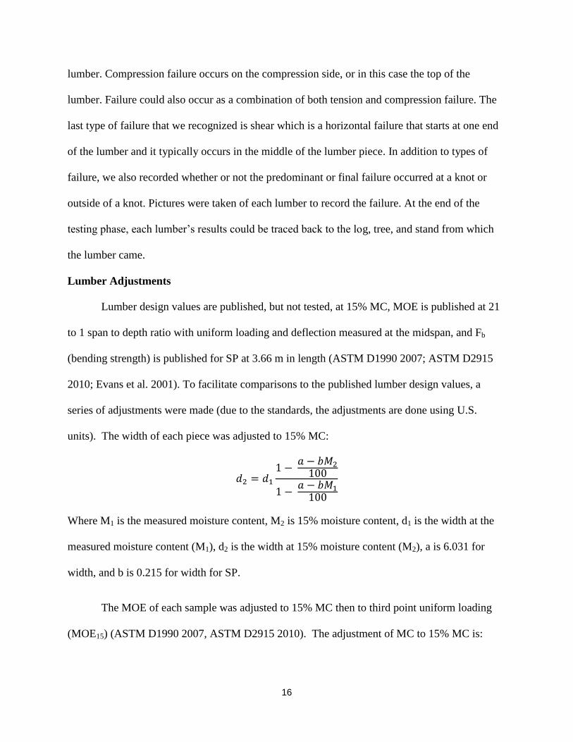
units). The width of each piece was adjusted to 15% MC:

Where M1 is the measured moisture content, M2 is 15% moisture content, d1 is the width at the

measured moisture content (M1), d2 is the width at 15% moisture content (M2), a is 6.031 for

width, and b is 0.215 for width for SP.

The MOE of each sample was adjusted to 15% MC then to third point uniform loading

(MOE15) (ASTM D1990 2007, ASTM D2915 2010). The adjustment of MC to 15% MC is:

17

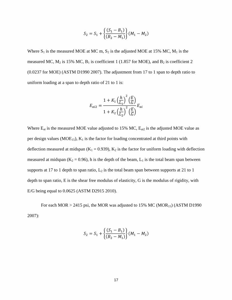
Where S1 is the measured MOE at MC m, S2 is the adjusted MOE at 15% MC, M1 is the

measured MC, M2 is 15% MC, B1 is coefficient 1 (1.857 for MOE), and B2 is coefficient 2

(0.0237 for MOE) (ASTM D1990 2007). The adjustment from 17 to 1 span to depth ratio to

uniform loading at a span to depth ratio of 21 to 1 is:

Where Eai is the measured MOE value adjusted to 15% MC, Eai2 is the adjusted MOE value as

per design values (MOE15), K1 is the factor for loading concentrated at third points with

deflection measured at midspan (K1 = 0.939), K2 is the factor for uniform loading with deflection

measured at midspan (K2 = 0.96), h is the depth of the beam, L1 is the total beam span between

supports at 17 to 1 depth to span ratio, L2 is the total beam span between supports at 21 to 1

depth to span ratio, E is the shear free modulus of elasticity, G is the modulus of rigidity, with

E/G being equal to 0.0625 (ASTM D2915 2010).

For each MOR > 2415 psi, the MOR was adjusted to 15% MC (MOR15) (ASTM D1990

2007):

18

Where S1 is the measured MOR at MC m, S2 is the adjusted MOR at 15% MC, M1 is the

measured MC, M2 is 15% MC, B1 is coefficient 1 (2415 for MOR), and B2 is coefficient 2 (40

for MOR) (ASTM D1990 2007).

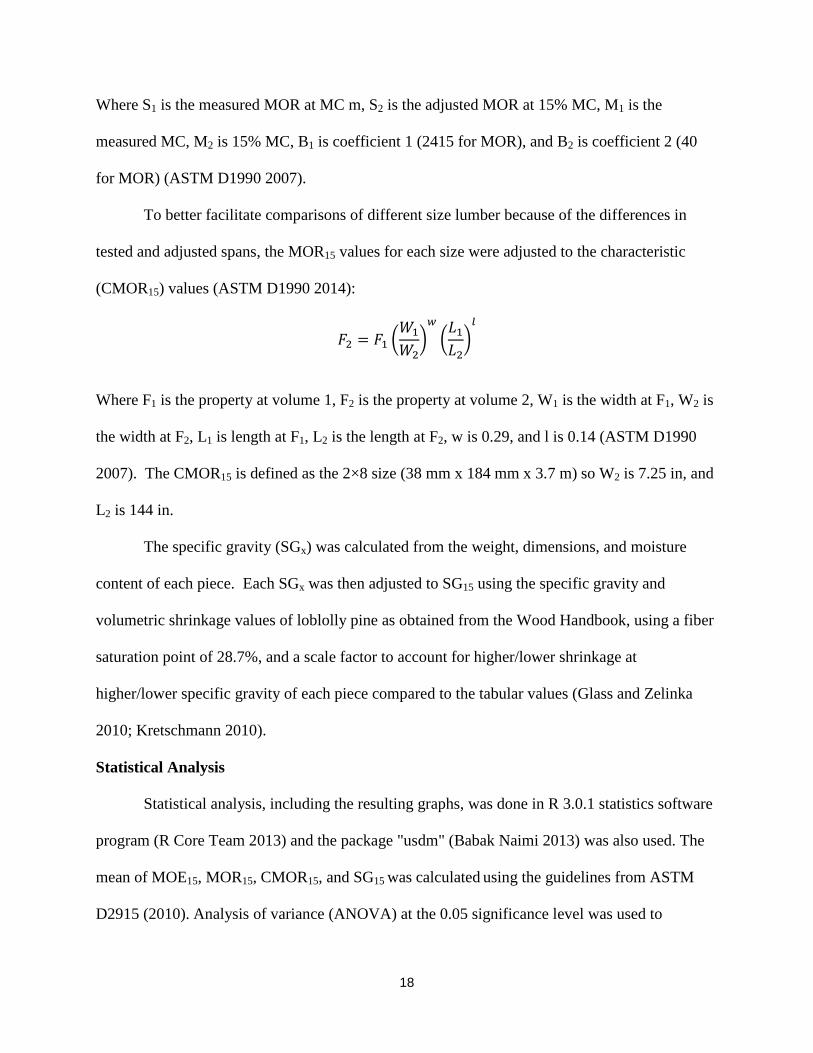
To better facilitate comparisons of different size lumber because of the differences in

tested and adjusted spans, the MOR15 values for each size were adjusted to the characteristic

(CMOR15) values (ASTM D1990 2014):

Where F1 is the property at volume 1, F2 is the property at volume 2, W1 is the width at F1, W2 is

the width at F2, L1 is length at F1, L2 is the length at F2, w is 0.29, and l is 0.14 (ASTM D1990

2007). The CMOR15 is defined as the 2×8 size (38 mm x 184 mm x 3.7 m) so W2 is 7.25 in, and

L2 is 144 in.

The specific gravity (SGx) was calculated from the weight, dimensions, and moisture

content of each piece. Each SGx was then adjusted to SG15 using the specific gravity and

volumetric shrinkage values of loblolly pine as obtained from the Wood Handbook, using a fiber

saturation point of 28.7%, and a scale factor to account for higher/lower shrinkage at

higher/lower specific gravity of each piece compared to the tabular values (Glass and Zelinka

2010; Kretschmann 2010).

Statistical Analysis

Statistical analysis, including the resulting graphs, was done in R 3.0.1 statistics software

program (R Core Team 2013) and the package "usdm" (Babak Naimi 2013) was also used. The

mean of MOE15, MOR15, CMOR15, and SG15 was calculated using the guidelines from ASTM

D2915 (2010). Analysis of variance (ANOVA) at the 0.05 significance level was used to

19

determine significant differences in acoustic velocity by log position and by grade. It was also

used to determine differences in grade produced by stand and by log, and differences in MOE15,

MOR15, and CMOR15 by log and by grade. ANOVA was also used to determine if MOE15

showed significant differences by stand. Tukey’s test was also used to further determine which

factors of a variable showed significant differences. Linear models were used to predict MOE15

(butt to log 3, butt to log 2, and individual logs) from Hitman values based on an in-woods

approach and a mill approach. A more complex model that used Specific Gravity (SG15) along

with the Hitman values was also considered for each of the scenarios. R2 was calculated to find

the model which best predicts MOE.

20

CHAPTER 4

RESULTS AND DISCUSSION

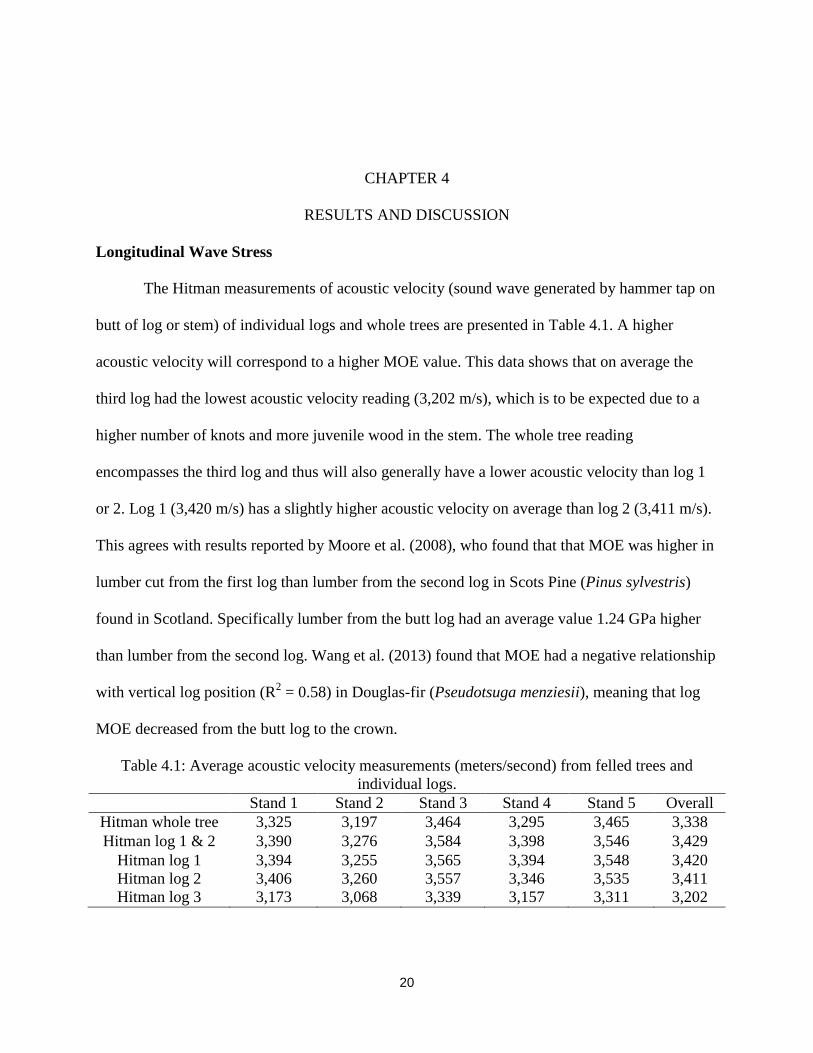
Longitudinal Wave Stress

The Hitman measurements of acoustic velocity (sound wave generated by hammer tap on

butt of log or stem) of individual logs and whole trees are presented in Table 4.1. A higher

acoustic velocity will correspond to a higher MOE value. This data shows that on average the

third log had the lowest acoustic velocity reading (3,202 m/s), which is to be expected due to a

higher number of knots and more juvenile wood in the stem. The whole tree reading

encompasses the third log and thus will also generally have a lower acoustic velocity than log 1

or 2. Log 1 (3,420 m/s) has a slightly higher acoustic velocity on average than log 2 (3,411 m/s).

This agrees with results reported by Moore et al. (2008), who found that that MOE was higher in

lumber cut from the first log than lumber from the second log in Scots Pine (Pinus sylvestris)

found in Scotland. Specifically lumber from the butt log had an average value 1.24 GPa higher

than lumber from the second log. Wang et al. (2013) found that MOE had a negative relationship

with vertical log position (R2 = 0.58) in Douglas-fir (Pseudotsuga menziesii), meaning that log

MOE decreased from the butt log to the crown.

Table 4.1: Average acoustic velocity measurements (meters/second) from felled trees and

individual logs.

Stand 1 Stand 2 Stand 3 Stand 4 Stand 5 Overall

Hitman whole tree 3,325 3,197 3,464 3,295 3,465 3,338

Hitman log 1 & 2 3,390 3,276 3,584 3,398 3,546 3,429

Hitman log 1 3,394 3,255 3,565 3,394 3,548 3,420

Hitman log 2 3,406 3,260 3,557 3,346 3,535 3,411

Hitman log 3 3,173 3,068 3,339 3,157 3,311 3,202

21

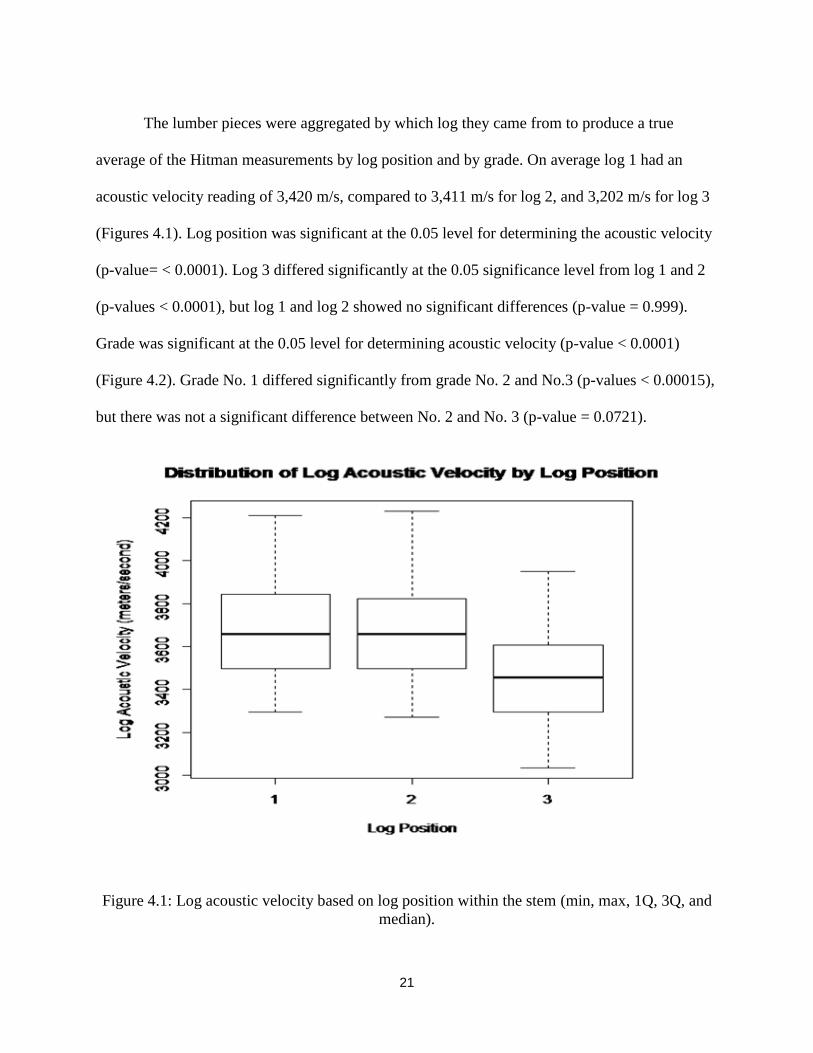
The lumber pieces were aggregated by which log they came from to produce a true

average of the Hitman measurements by log position and by grade. On average log 1 had an

acoustic velocity reading of 3,420 m/s, compared to 3,411 m/s for log 2, and 3,202 m/s for log 3

(Figures 4.1). Log position was significant at the 0.05 level for determining the acoustic velocity

(p-value= < 0.0001). Log 3 differed significantly at the 0.05 significance level from log 1 and 2

(p-values < 0.0001), but log 1 and log 2 showed no significant differences (p-value = 0.999).

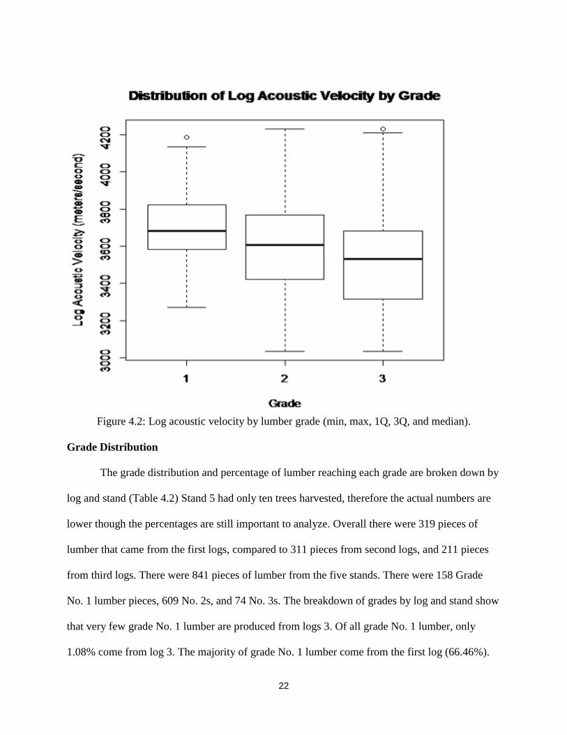
Grade was significant at the 0.05 level for determining acoustic velocity (p-value < 0.0001)

(Figure 4.2). Grade No. 1 differed significantly from grade No. 2 and No.3 (p-values < 0.00015),

but there was not a significant difference between No. 2 and No. 3 (p-value = 0.0721).

Figure 4.1: Log acoustic velocity based on log position within the stem (min, max, 1Q, 3Q, and

median).

22

Figure 4.2: Log acoustic velocity by lumber grade (min, max, 1Q, 3Q, and median).

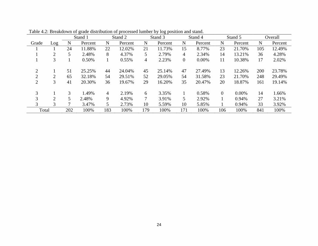
Grade Distribution

The grade distribution and percentage of lumber reaching each grade are broken down by

log and stand (Table 4.2) Stand 5 had only ten trees harvested, therefore the actual numbers are

lower though the percentages are still important to analyze. Overall there were 319 pieces of

lumber that came from the first logs, compared to 311 pieces from second logs, and 211 pieces

from third logs. There were 841 pieces of lumber from the five stands. There were 158 Grade

No. 1 lumber pieces, 609 No. 2s, and 74 No. 3s. The breakdown of grades by log and stand show

that very few grade No. 1 lumber are produced from logs 3. Of all grade No. 1 lumber, only

1.08% come from log 3. The majority of grade No. 1 lumber come from the first log (66.46%).

23

Also for most stands, logs 1-3 produce grade No. 2 logs at the highest rate. The exception to this

rule is from Stand 5, which produced a higher percentage of grade No. 1 lumber from the first

log.

24

Table 4.2: Breakdown of grade distribution of processed lumber by log position and stand.

Stand 1 Stand 2 Stand 3 Stand 4 Stand 5 Overall

Grade Log N Percent N Percent N Percent N Percent N Percent N Percent

1 1 24 11.88% 22 12.02% 21 11.73% 15 8.77% 23 21.70% 105 12.49%

1 2 5 2.48% 8 4.37% 5 2.79% 4 2.34% 14 13.21% 36 4.28%

1 3 1 0.50% 1 0.55% 4 2.23% 0 0.00% 11 10.38% 17 2.02%

2 1 51 25.25% 44 24.04% 45 25.14% 47 27.49% 13 12.26% 200 23.78%

2 2 65 32.18% 54 29.51% 52 29.05% 54 31.58% 23 21.70% 248 29.49%

2 3 41 20.30% 36 19.67% 29 16.20% 35 20.47% 20 18.87% 161 19.14%

3 1 3 1.49% 4 2.19% 6 3.35% 1 0.58% 0 0.00% 14 1.66%

3 2 5 2.48% 9 4.92% 7 3.91% 5 2.92% 1 0.94% 27 3.21%

3 3 7 3.47% 5 2.73% 10 5.59% 10 5.85% 1 0.94% 33 3.92%

Total 202 100% 183 100% 179 100% 171 100% 106 100% 841 100%

25

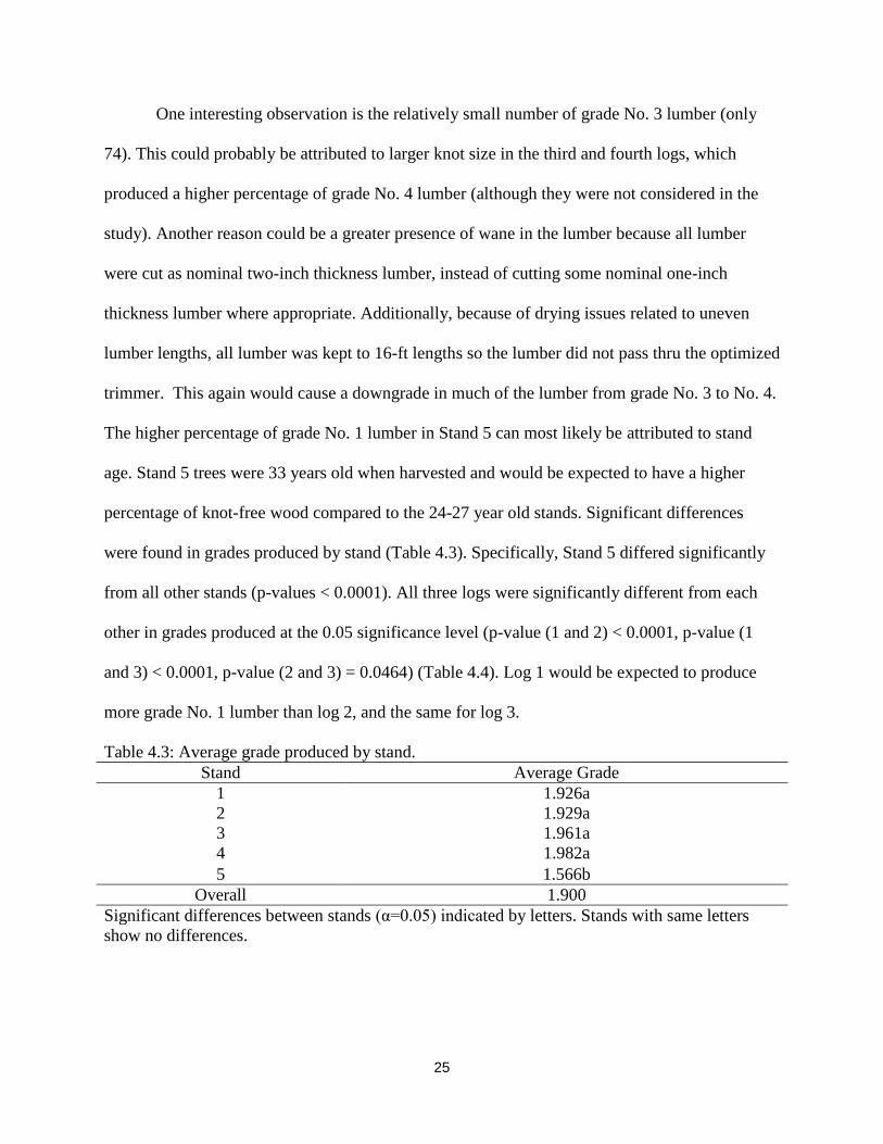
One interesting observation is the relatively small number of grade No. 3 lumber (only

74). This could probably be attributed to larger knot size in the third and fourth logs, which

produced a higher percentage of grade No. 4 lumber (although they were not considered in the

study). Another reason could be a greater presence of wane in the lumber because all lumber

were cut as nominal two-inch thickness lumber, instead of cutting some nominal one-inch

thickness lumber where appropriate. Additionally, because of drying issues related to uneven

lumber lengths, all lumber was kept to 16-ft lengths so the lumber did not pass thru the optimized

trimmer. This again would cause a downgrade in much of the lumber from grade No. 3 to No. 4.

The higher percentage of grade No. 1 lumber in Stand 5 can most likely be attributed to stand

age. Stand 5 trees were 33 years old when harvested and would be expected to have a higher

percentage of knot-free wood compared to the 24-27 year old stands. Significant differences

were found in grades produced by stand (Table 4.3). Specifically, Stand 5 differed significantly

from all other stands (p-values < 0.0001). All three logs were significantly different from each

other in grades produced at the 0.05 significance level (p-value (1 and 2) < 0.0001, p-value (1

and 3) < 0.0001, p-value (2 and 3) = 0.0464) (Table 4.4). Log 1 would be expected to produce

more grade No. 1 lumber than log 2, and the same for log 3.

Table 4.3: Average grade produced by stand.

Stand Average Grade

1 1.926a

2 1.929a

3 1.961a

4 1.982a

5 1.566b

Overall 1.900

Significant differences between stands (α=0.05) indicated by letters. Stands with same letters

show no differences.

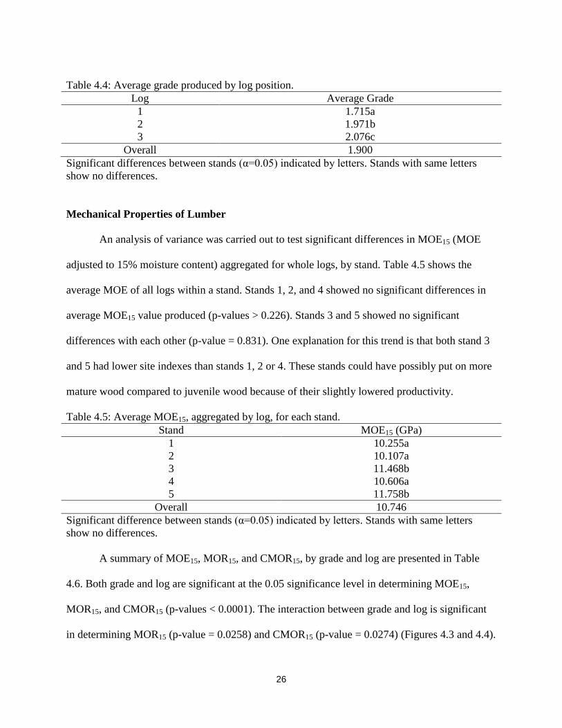
26

Table 4.4: Average grade produced by log position.

Log Average Grade

1 1.715a

2 1.971b

3 2.076c

Overall 1.900

Significant differences between stands (α=0.05) indicated by letters. Stands with same letters

show no differences.

Mechanical Properties of Lumber

An analysis of variance was carried out to test significant differences in MOE15 (MOE

adjusted to 15% moisture content) aggregated for whole logs, by stand. Table 4.5 shows the

average MOE of all logs within a stand. Stands 1, 2, and 4 showed no significant differences in

average MOE15 value produced (p-values > 0.226). Stands 3 and 5 showed no significant

differences with each other (p-value = 0.831). One explanation for this trend is that both stand 3

and 5 had lower site indexes than stands 1, 2 or 4. These stands could have possibly put on more

mature wood compared to juvenile wood because of their slightly lowered productivity.

Table 4.5: Average MOE15, aggregated by log, for each stand.

Stand MOE15 (GPa)

1 10.255a

2 10.107a

3 11.468b

4 10.606a

5 11.758b

Overall 10.746

Significant difference between stands (α=0.05) indicated by letters. Stands with same letters

show no differences.

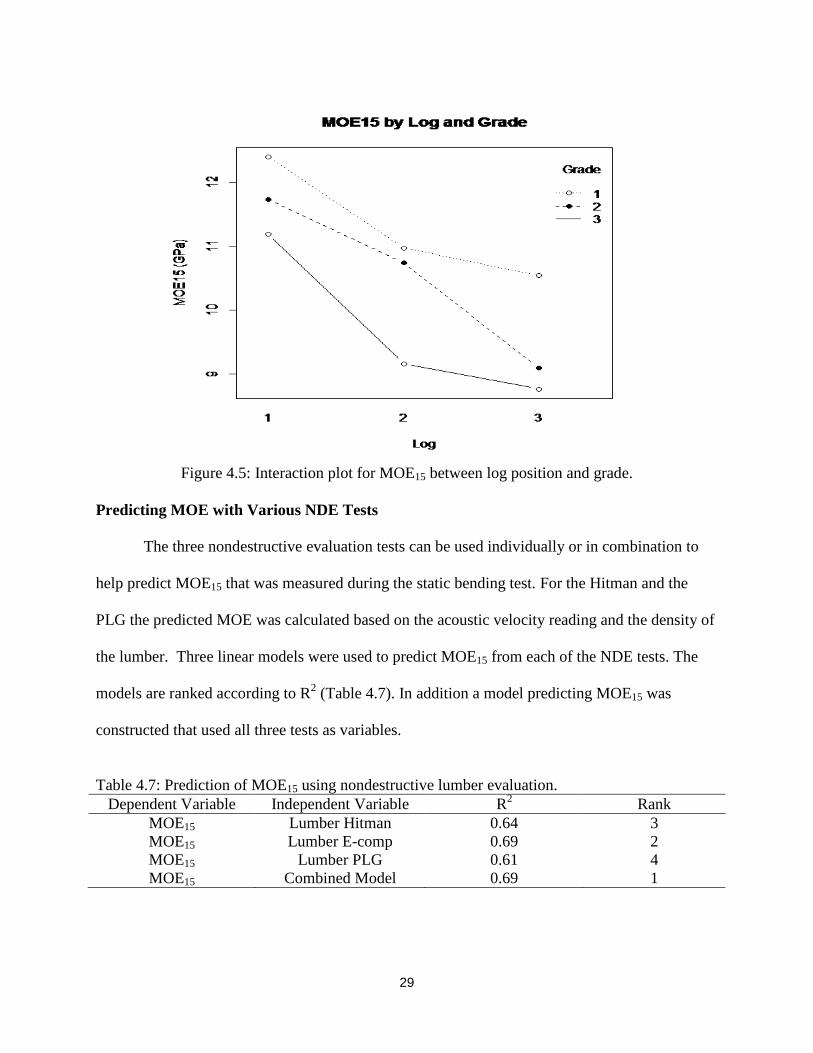
A summary of MOE15, MOR15, and CMOR15, by grade and log are presented in Table

4.6. Both grade and log are significant at the 0.05 significance level in determining MOE15,

MOR15, and CMOR15 (p-values < 0.0001). The interaction between grade and log is significant

in determining MOR15 (p-value = 0.0258) and CMOR15 (p-value = 0.0274) (Figures 4.3 and 4.4).

27

This interaction is not significant in determining MOE15 (p-value = 0.907) (Figure 4.5). Grade

No. 1 lumber from log 3 has significantly higher MOR15, and CMOR15 values than do grades

No. 2 and No. 3 lumber from log 3 (Figures 4.3 and 4.4). The pattern of interactions between log

and grade appears to be decreasing MOR, MOE, and CMOR from grade No. 1 to No.3, and

decreasing MOR, MOE, and CMOR from lumber in the butt log to lumber that comes from

higher in the stem. Grade No. 1 logs do not appear to follow the same pattern. Instead they

remain constant or slightly increase in strength properties from the second log to the third log.

These observations do not follow the general pattern of decreasing strength and stiffness from

the butt log to the crown that Wang et al. (2012) found in Douglas-fir.

This could be attributed to less variability in grade No. 1 material due to smaller knot size or an

insufficient sample size of grade No. 1 material from log 2 and 3.

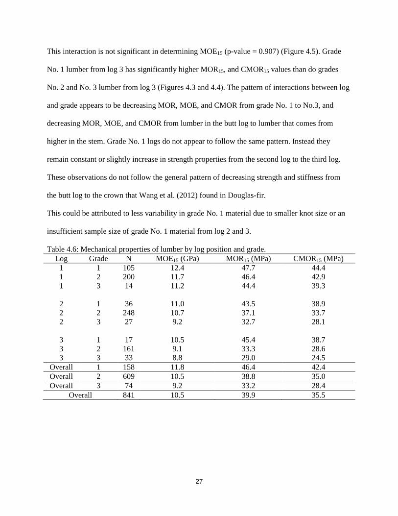
Table 4.6: Mechanical properties of lumber by log position and grade.

Log Grade N MOE15 (GPa) MOR15 (MPa) CMOR15 (MPa)

1 1 105 12.4 47.7 44.4

1 2 200 11.7 46.4 42.9

1 3 14 11.2 44.4 39.3

2 1 36 11.0 43.5 38.9

2 2 248 10.7 37.1 33.7

2 3 27 9.2 32.7 28.1

3 1 17 10.5 45.4 38.7

3 2 161 9.1 33.3 28.6

3 3 33 8.8 29.0 24.5

Overall 1 158 11.8 46.4 42.4

Overall 2 609 10.5 38.8 35.0

Overall 3 74 9.2 33.2 28.4

Overall 841 10.5 39.9 35.5

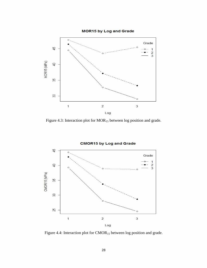
28

Figure 4.3: Interaction plot for MOR15 between log position and grade.

Figure 4.4: Interaction plot for CMOR15 between log position and grade.

29

Figure 4.5: Interaction plot for MOE15 between log position and grade.

Predicting MOE with Various NDE Tests

The three nondestructive evaluation tests can be used individually or in combination to

help predict MOE15 that was measured during the static bending test. For the Hitman and the

PLG the predicted MOE was calculated based on the acoustic velocity reading and the density of

the lumber. Three linear models were used to predict MOE15 from each of the NDE tests. The

models are ranked according to R2 (Table 4.7). In addition a model predicting MOE15 was

constructed that used all three tests as variables.

Table 4.7: Prediction of MOE15 using nondestructive lumber evaluation.

Dependent Variable Independent Variable R2

Rank

MOE15 Lumber Hitman 0.64 3

MOE15 Lumber E-comp 0.69 2

MOE15 Lumber PLG 0.61 4

MOE15 Combined Model 0.69 1

30

The combined model and the E-computer model had the highest R2 values (0.69) of any

of the models. One reason that the E-computer might have outperformed the Hitman and the

PLG reading is because the test design mimics a bending test whereas the acoustic velocity

instruments due not. All three tests were relatively easy to set up and conduct, although the

Hitman requires the least amount of equipment and handling because the test is conducted from

only one end of the lumber.

Modeling MOE from Lumber NDE

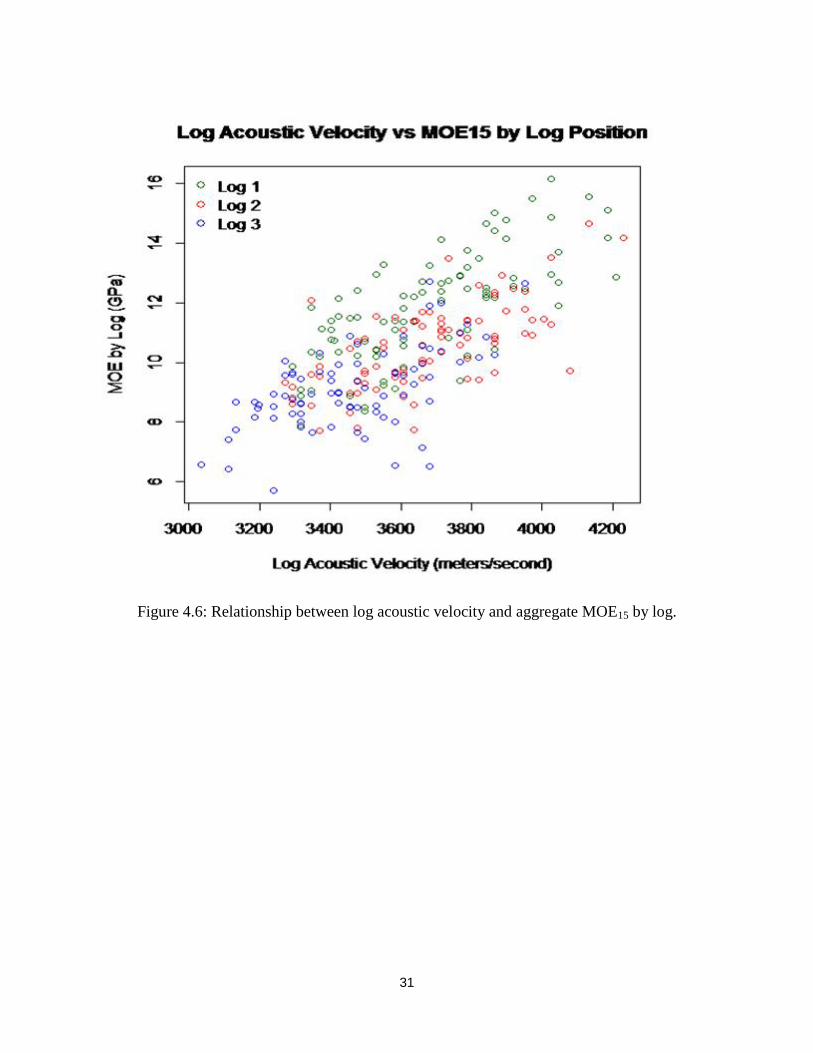
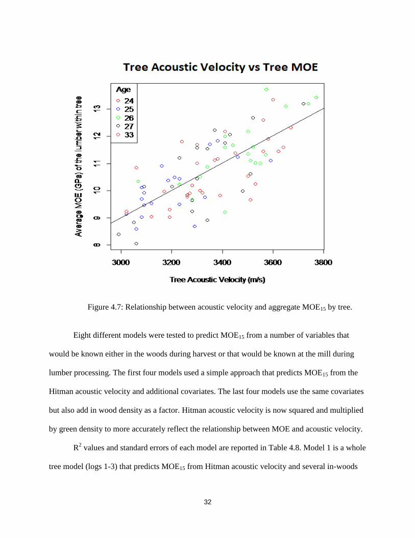
The relationship between MOE15 and Hitman acoustic velocity of individual logs is

presented in Figure 4.6. R2 = 0.52. The relationship between MOE15 of all of the lumber in an

individual tree and tree acoustic velocity is found in Figure 4.7. R2 = 0.55. The whole tree model

has a slightly higher coefficient of determination and this relationship appears similar across all

ages. This is slightly surprising because whole tree acoustic velocity measurements would be

expected to have more variation than log velocity due to a greater distance that the sound waves

have to travel to take a reading.

31

Figure 4.6: Relationship between log acoustic velocity and aggregate MOE15 by log.

32

Figure 4.7: Relationship between acoustic velocity and aggregate MOE15 by tree.

Eight different models were tested to predict MOE15 from a number of variables that

would be known either in the woods during harvest or that would be known at the mill during

lumber processing. The first four models used a simple approach that predicts MOE15 from the

Hitman acoustic velocity and additional covariates. The last four models use the same covariates

but also add in wood density as a factor. Hitman acoustic velocity is now squared and multiplied

by green density to more accurately reflect the relationship between MOE and acoustic velocity.

R2 values and standard errors of each model are reported in Table 4.8. Model 1 is a whole

tree model (logs 1-3) that predicts MOE15 from Hitman acoustic velocity and several in-woods

33

covariates to simulate what a logger or forester might know about the trees during harvest.

Model 2 is a whole tree model that predicts MOE15 from Hitman acoustic velocity and several

mill covariates to simulate what information a lumber mill would have during lumber processing.

Model 3 uses the same variables as model 2 but simply uses logs 1 and 2 due to the large branch

size and other defects present in many of the third logs. Model 4 is an individual log model from

the mill perspective to better show the relationship of MOE15 to each log position. Models 5-8

are replicates of the first four except that acoustic velocity is used along with wood density to

calculate a Hitman MOE, which is used to predict MOE15.

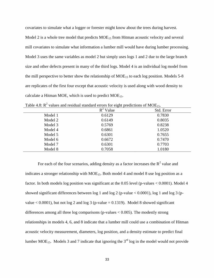
Table 4.8: R2 values and residual standard errors for eight predictions of MOE15.

R2 Value Std. Error

Model 1 0.6129 0.7830

Model 2 0.6149 0.8035

Model 3 0.5769 0.8238

Model 4 0.6861 1.0520

Model 5 0.6301 0.7655

Model 6 0.6672 0.7470

Model 7 0.6301 0.7703

Model 8 0.7058 1.0180

For each of the four scenarios, adding density as a factor increases the R2 value and

indicates a stronger relationship with MOE15. Both model 4 and model 8 use log position as a

factor. In both models log position was significant at the 0.05 level (p-values < 0.0001). Model 4

showed significant differences between log 1 and log 2 (p-value < 0.0001), log 1 and log 3 (p-

value < 0.0001), but not log 2 and log 3 (p-value = 0.1319). Model 8 showed significant

differences among all three log comparisons (p-values < 0.005). The modestly strong

relationships in models 4, 6, and 8 indicate that a lumber mill could use a combination of Hitman

acoustic velocity measurement, diameters, log position, and a density estimate to predict final

lumber MOE15. Models 3 and 7 indicate that ignoring the 3rd

log in the model would not provide

34

a better estimate of MOE15. On average, using log and tree characteristics that could be easily

measured at a mill provide modestly better estimates of MOE15 than using information that

would be readily available to loggers or procurement foresters.

35

CHAPTER 5

CONCLUSIONS

Due to the recent reduction in southern pine design values, it is important to determine

the specific cause of these downward adjustments. The results of this study suggest that log

position, age, and tree size all play a critical role in determining lumber MOE and MOR, or

strength and stiffness. A reduction in MOE and MOR can most likely be attributed to an increase

in the percentage of juvenile wood. Trees that were grown under intensive management practices

typically have wider growth rings and are harvested at a younger age than in the past. Trees that

grow faster have higher percentages of juvenile core wood which is usually less stiff and weaker

than mature wood.

The results from this study suggest that lumber cut from intensively grown mature pine

stands in the Coastal Plain of Georgia show significant differences in acoustic stiffness

properties based on log position and the grade of processed lumber. Knowing which log the

lumber came from can help predict final MOE and MOR. The results from this study agree with

Moore et al. (2008) who found that MOE decreases as you move up the stem. Also using log

acoustic wavelength tests (Hitman), as well knowing the age, DBH, log diameters, and log

position, the MOE of lumber can be reasonably predicted.

Portable acoustic wavelength measuring devices could potentially be used, along with

commonly known tree properties, to predict MOE and MOR of lumber. This could lead to more

advanced product sorting at harvesting sites to insure that lower quality logs that would produce

less desirable lumber are not sent to sawtimber mills. Alternately product sorting could

potentially be used to charge a premium price on logs that are known to have high acoustic

36

velocity and that can be expected to produce lumber that exceed the current southern pine design

value standards.

37

REFERENCES

Antony, F., J. Lewis, L. R. Schimleck, A. Clark, R.A. Souter, R.F. Daniels. 2011. Regional

variation in wood modulus of elasticity (stiffness) and modulus of rupture (strength) of

planted loblolly pine in the United States. Canadian Journal of Forest Research 41(7):

1522-1533.

ASTM International. 2006. ASTM D245-06: Standard practice for establishing structural grades

and related allowable properties for visually graded lumber. West Conshohocken, PA.

ASTM International. 2007. ASTM D1990-07: Standard practice for establishing allowable

properties for visually-graded dimension lumber from in-grade tests of full-size

specimens. West Conshohocken, PA.

ASTM International. 2010. ASTM D2915-10: Standard practice for evaluating allowable

properties for grades of structural lumber. West Conshohocken, PA.

ASTM International. 2013. ASTM D4761-13: Standard test methods for mechanical properties

of lumber and wood-base structural material. West Conshohocken, PA.

ASTM International. 2014. ASTM D198-14: Standard test methods of static tests of lumber in

structural sizes. West Conshohocken, PA.

ASTM International. 2014. ASTM D1990-14: Standard practice for establishing allowable

properties for visually-graded dimension lumber from in-grade tests of full-size

specimens. West Conshohocken, PA.

Baldwin Jr., V.C., K.D. Peterson, A. Clark III, R.B. Ferguson, M.R. Strub, and D.R. Bower.

2000. The effects of spacing and thinning on stand and tree characteristics of 38-year-old

loblolly pine. Forest Ecology and Management. 137(1-3): 91-102.

38

Bettinger, P., M. Clutter, J. Siry, M. Kane, and J. Pait. 2009. Broad implications of southern

United States pine clonal forestry on planning and management of forests. The

International Forestry Review. 11(3): 331-345.

Biblis, E.J., R. Brinker, and H.F. Carino. 1995. Effect of stand density on flexural properties of

lumber from two 35-year-old loblolly pine plantations. Wood and Fiber Science. 29(4):

29-33.

Biblis, E.J., R. Brinker, H. Carino, and C.W. McKee. 1993. Effect of stand age on flexural

properties and grade compliance of lumber from loblolly pine plantation timber. Forest

Products Journal. 43(2): 23-28.

Carter, P., S. Chauhan, and J. Walker. 2006. Sorting logs and lumber for stiffness using Director

HM200. Wood Fiber Science. 38(1): 49-54.

Clark, A. L. Jordan, L. Schimleck, and R.F. Daniels. 2008. Effect of initial planting spacing on

wood properties of unthinned loblolly pine at age 21. Forest Products Journal. 58(10):

78-83.

Cramer, S., D. Kretschmann, R. Lakes, and T. Schmidt. 2005. Earlywood and latewood elastic

properties in loblolly pine. Holzforchung. 59(5): 531-538.

Dahlen, J., P.D. Jones, R.D. Seale, and R. Shmulsky. 2012. Bending strength and stiffness of in-

grade Douglas-fir and southern pine No. 2 2x4 lumber. Canadian Journal for Forest

Research. 42: 858-867.

Dahlen, J., P.D. Jones, R.D. Seale, and R. Shmulsky. 2014. Bending strength and stiffness of

wide dimension southern pine No.2 lumber. European Journal of Wood Products.

72:759-768.

39

Downes, G.M., J.G. Nyakuengama, R. Evans, R. Northway, P Blakemore, R.L. Dickson, and M.

Lausberg. 2002. Relationship between wood density, microfibril angle, and stiffness in

thinned and fertilized Pinus radiata. IAWA. 23(3): 253-265.

Evans, J., D. Kretschmann, V. Herian, and D. Green. 2001. Procedures for developing

allowable properties for a single species under ASTM D1990 and computer programs

useful for the calculations. Madison, WI: USDA Forest Service. FPL-GTR-126.

Glass S.V. and S.L. Zelinka. 2010. Wood Handbook: Moisture relations and physical properties

of wood. Madison, WI: USDA Forest Service. FPL-GTR-190. p. 4.1-4.19.

Grabianowski, M., B. Manley, J. Walker. 2006. Acoustic measurement on standing trees, logs,

and green lumber. Wood Science and Technology. 40(3):205-216.

Green, D.W. and J.W. Evans. 1988. Mechanical properties of visually graded lumber. Volume

1: A summary; Volume 2: Douglas-fir-Larch; Volume 4: Southern Pine. National

Technical Information Service. PB-88-159-389; PB-88-159-397; PB-88-158-413.

Groover, A., M. Devey, T. Fiddler, J. Lee, R. Megraw, T. Mitchel-Olds, B. Sherman, S. Vujcic,

C. Williams, and D. Neale. 1994. Identification of quantitative trait loci influencing wood

specific gravity in an outbred pedigree of loblolly pine. Genetics. 138(4): 1293-1300.

Jokela, E.J., T.A Martin, and J.G. Vogel. 2010. Twenty-five years of intensive forest

management with southern pines: important lessons learned. Journal of Forestry. 108(7):

338-347.

Kretschmann D.E. 2010. Mechanical properties of wood. Wood handbook: Wood as an

engineering material: Madison, WI: USDA Forest Service. FPL-GTR-190. p. 5.1-5.46.

40

Kretschmann, D. E., B.A. Bendsten. 1991. Ultimate tensile stress and modulus of elasticity of

fast-grown plantation loblolly pine lumber. Madison, WI: USDA Forest Service, FPL.

24(2):189-203.

Kretschmann, D.E., H.A. Alden, S. Verrill. 1998. Variations of microfibril angle in loblolly pine:

Comparison of iodine crystallization and X-ray diffraction techniques. In: Microfibril

Angle in Wood. Ed. Butterfield, B.G. University of Canterbury Press, Christchurch, New

Zealand. pp. 157–176.

Larson P.R., D.E. Kretschmann, A. Clark II, and J.G. Isebrands. 2001. Formation and properties

of juvenile wood in southern pines: A synopsis. Madison, WI: USDA Forest Service,

Forest Products Laboratory. 42 p.

Lasserre, J.P., E.G. Mason, M.S. Watt, and J.R. Moore. 2009. Influence of initial planting

spacing and genotype on microfibril angle, wood density, fibre properties and modulus of

elasticity in Pinus radiata (D. Don) corewood. Forest Ecology and Management. 258(9):

1924-1931.

Löf, M., D.C. Dey, R.M. Navarro, D.F. Jacobs. 2012. Mechanical site preparation for forest

restoration. New Forests. 43:825–848.

Moore, J., A. Lyon, G. Searles, S. Lehneke, and E. Macdonald. 2008. Scots pine timber quality

in North Scotland. Report on the investigation of mechanical properties of structural

timber from three stands. Center for Timber Engineering. Edinburgh, Scotland.

Mora, C.R., L.R. Schimleck, F. Isik, J.M, Mahon, Jr., A. Clark, III, and R.F. Daniels. 2009.

Relationships between acoustic variables and different measures of stiffness in standing

Pinus taeda trees. Canadian Journal of Forest Resources. 39: 1421-1429.

41

Naimi, B. 2013. usdm: Uncertainty analysis for species distribution models. R package version

1.1-12. http://CRAN.R-project.org/package=usdm

Pellerin, R.F. and R.J. Ross. 2002. Nondestructive evaluation of wood. Madison, WI: Forest

Products Society.

R Core Team. 2013. R: A language and environment for statistical computing. R Foundation for

Statistical Computing, Vienna, Austria. URL http://www.R-project.org/.

Ross, R.J., E.A. Geske, G.L. Larson, and J.F. Murphy.1991. Transverse vibration nondestructive

testing using a personal computer. Research Paper FPL-RP-502. USDA Forest Service,

Forest Products Laboratory, Madison, WI.

Roth, B. E., X. Li, D. A. Huber, and G.F. Peter. 2007. Effects of management intensity,

genetics and planting density on wood stiffness in a plantation of juvenile loblolly pine in

the southeastern USA. Forest Ecology and Management. 246(2-3): 155-162.

Southern Forest Products Association. 2011.

<http://www.southernpine.com/app/uploads/DesignValueForumReport.pdf/>.

Accessed September 10, 2012.

Southern Forest Products Association. 2012.

<http://www.southernpine.com/transition-new- design-values-effective-june-1-2012/>.

Accessed September 10, 2012.

Southern Forest Products Association. 2013.

<http://www.southernpine.com/alsc-approves-new-design-values-southern-pine-

lumber/>. Accessed June 30, 2014.

42

Stanturf, J.A., R.C. Kellison, F.S. Broerman, and S.B. Jones. 2003. Innovation and forest

industry: Domesticating the pine forests of the southern United States, 1920-1999. Forest

Policy and Economics. 5(4): 407-419.

Wang, X. 2013. Acoustic measurements on trees and logs: a review and analysis. Wood Science

Technology. 47: 965-975.

Wang, X., R.J. Ross, J.A. Mattson, J.R. Erickson, J.W. Forsman, E.A. Geske, and M.A. Wehr.

2002. Nondestructive evaluation techniques for assessing modulus of elasticity and

stiffness of small-diameter logs. Forest Products Journal. 52(2): 79-85.

Wang, X., R.J. Ross, M.H. McClellan, R.J. Barbour, J.R. Erickson, J.W. Forsman, and G.D.

McGinnis. 2001. Nondestructive evaluation of standing trees with a stress wave method.

Wood and Fiber Science. 33(4): 522-533.

Wang, X., S. Verrill, E. Lowell, R.J. Ross, V.L. Herian. 2013 Acoustic sorting models for

improved log segregation. Wood and Fiber Science. 45(4): 343-352.

Watt, M.S., G.M. Downes, D. Whitehead, E.G. Mason, B. Richardson, J.C. Grace, and J.R.

Moore. 2005. Wood properties of juvenile Pinus radiata growing in the presence and

absence of competing understory vegetation at a dryland site. Trees. 19(5): 580-586.

Wear, D., and J. Greis. 2002. Southern forest resource assessment. US Forest Service General

Technical Report. SRS-53, Asheville, NC. 635 p.

Zhao, D., M. Kane, and B.E. Borders. 2011. Growth responses to planting density and

management intensity in loblolly pine plantations in the southeastern USA Lower Coastal

Plain. Annals of Forest Science. 68(3): 625-635.