ping · Number 44, JournalVolume ofXXIVPhilippine, No. 2,DevelopmentSecond Semester 1997 ping...

Journal of Philippine Development pingNumber 44, Volume XXIV, No. 2, Second Semester 1997

SIMULATING THE EFFECTS OF GATT-UR/WTOON THE PHILIPPINE ECONOMY 1

Caesar B. Cororaton

The Philippine economy may be affected by the new GATT/WTO inthree possible ways: (a) through the changes in the tariff structure ofthe economy as a result of the commitments of the Philippines duringthe Uruguay Round (UR); (b) through the expansion of the world tradeas both developed countries (DCs) and less developed countries (LDCS)

adjust their respective trade protection structures; and (c) through thechanges in the world export and import prices as a result of therealignment in trade and non-trade barriers (NTBs) existing in both DCs

and LDCs. The objective of this paper is to simulate the possible impactof these changes on the local economy using a Philippine economicmodel. Specifically, it will attempt to determine whether the effects willbe favorable at the macroeconomic level and progressive in terms ofincome distribution. Furthermore, the paper will also look into thesectoral output effects,

The model used tosimulate these changes is a computable generalequilibrium (CGE) model of the Philippine economy called the APEXmodel. The model can adequately capture the intersectoral reallocation

movements of outputs and factors among the different industries andsectors of the economy as a result of changes in the world economy(see Appendix).

The paper is divided into seven sections and one appendix. SectionI discusses the country's trade program, with particular emphasis on

1. Part of the discussion in the paper is based on "The Impact of GATT/Uruguay Roundon Employment: Prospects for the Philippines". May 1995, ILO-SEAPAT. However,revisions have been made in the simulations, incorporating new information about thetariff system in the Philippines and projections on the world economy.

192 JOURNAL OF PHILIPPINEDEVELOPMENT

Executive Order (EO) 470. Section II discusses briefly the commitments

of the Philippines in terms of changes in tariff rates, including the initialbound rates set in 1995 and the final bound rates in 2004. Section III

discusses the effective changes in tariff rates both in the agricultural

and industrial sectors of the economy, putting in perspective theongoing trade program of the government. It will specifically determinewhether or not at specific industry level the effective change will lead toincreases in protection, i.e., relative to the committed initial bound ratesset in 1995 whether the present nominal tariff protection rate of theindustry is lower or higher. Section IV discusses three sets ofprojections on the impact of the UR on the world economy. Theseprojections_are used to compute for the effects on the Philippineeconomy. Section V discusses the assumptions made in simulating theGATT/UR effects on the local economy. Section VI summarizes theresults of the simulation exercises conducted. The discussion will focus

on the following results: (i) changes in general macroeconomic variablesto see whether these are sustainable or not; (2) income distribution

effects; and (3) industry output effects. Section VII gives a brief

summary. Lastly, the Appendix gives a summary of the importantfeatures of the APEX model.

THE COUNTRY'S TRADE PROGRAM

The Philippines has been pursuing a series of unilateral tradeliberalization programs. For example, in 1981 the government embarkedon a five-year (1981-1985) tariff reduction program which resulted in

a general decline in the average nominal tariff level. However,because of the balance of payments crisis in the middle of the 1980s,the tariff reduction program was aborted. The same program,however, was later continued by the Aquino government starting1986 until the government embarked on another round of tariffreduction program in 1991 under EO 470.

EO 470 is a comprehensive program. It reduces the average tarifflevels and simplifies the tariff structure from a multi-tariff structure to astructure with only four tariff levels. In particular, the final rates clusteraround 3 percent, 10 percent, 20 percent, and 30 percent, as comparedto the previous structure where the rates ranged from 10 percent to 50percent.

CORORATON: SIMULATING THE EFFECTS OF GATT-UR/WTO 193

Under EO 470 the average nominal tariff is reduced from 28

percent (tariff level at the start of the program) to 20 percent at

the end of the tariff program in 1995, or a drop of 29 percent over

the five-year period (Table 1). Weighted by imports however, the

average tariff declines from 20 percent to 14 percent in 1995, or a

drop of 27 percent.

Table1. Nominal average and weighted average tariffs (in percent)

Nominal Average Tariffs (in percent)

Agriculture 35 35.94 33.89 31.83 29.92 28.02

Mining 14 10.99 11.30 10.72 10.72 10.72

Manufacturing 27 24.77 23.08 21.38 20.73 19.04

OVERALL 28 25.96 24.27 22,56 21.74 20,07

Weighted Average Tariffs (in percent)

470!' Year 3

Agriculture 22 23,80 23,48 23.15 22.85 22.56

Mining 11 9.69 10.12 10.05 10.05 10.05

Manufacturing 21 19.35 10.83 15.32 14.98 14.27

OVERALL 20 17.84 16.22 15.17 14.90 14.40

Source: Tariff Commission1991

Among the three major industrial sectors, manufacturing registers

the biggest reduction in average tariffs from 27 percent (unweighted) to

only 19 percent in 1 995, or a decline of 30 percent. For agriculture, the

average tariff declines from 36 percent to 28 percent in 1995, or a

decline of 22 percent.

Overall, the tariff reduction program of the early 1980s (which

was pursued in the second half of the 1980s) and EO 470 brought

down the number of regulated items from 1,924 in 1986 to just 183

at present.

194 JOURNAL OF PHILIPPINE DEVELOPMENT

COMMITTED BINDING TARIFF RATES

Table 2 presents the Philippine initial bound tariff rates set in 1995

and the final bound tariff rates in 2004. 2 To better appreciate these

binding commitments made, the table also includes the current tariff

rates applied in a few agricultural industries. 3 One should note that

these tariff rates are nominal in the sense that they do not include the

protection effects of the existing quantitative restrictions (QRs) and

other non-tariff barriers (NTBs) applied to selected industries. Also,

these rates are the 1995 programmed tariff rates under EO 470 whichis to terminate in 1995.

Table 2. Initial and final binding tariff rates

and percent change by sub-sectors

,, Final,Bound',,, I_rce,nt :,

' RateofDuW ' i: _,Rate, : Change :!

,:,:i,:}.....i:,i, ......,::i,,,,,:,:1,9.5,,:,,:,,,::' "zoo4,::;:i,",",',i ::"'!"' ' " ................ ':': "!":'i','" " :":

1. Irrigated rice 20 100 50 -50.002. Rain-fed rice 20 100 50 -50.003. Corn 20 100 50 -50.004. Coconut 50 70 50 -28.575. Sugarcane 50 90 50 -44.446. Fruits 50 60 40 -33.33

7. Vegetables 30 80 40 -50.008. Rootcrops 30 70 40 -42.869. Other

commercial crops 35 85 45 -47.0610. Hogs 20 35 27 -22.8611. Poultry 30 90 40 -55.5612. Other livestocks 10 20 15 -25.00

13. Agricultural services ....14. Marine fishing ....15. Inland fishing ....16. Forestry ....17. Crude oil ....

18. Other mining 10 15 50.00

Continued,.,

2. Note that these are the computed sectoral average tariff rates consistent to thesectoral breakdown of the production sector of the APEX model. The actual rates are forvery specific tariff lines,3. Tariff rates for the industrial sector are available but are not included in the table.


.,. con't. Table 2

'" i .... Current A:ppli_ |:_Jnt_al:!Bound Final Bound Percent

:Su_s_ors ' Rate of'DuW "i' Rate Rate Change:,, '!;,!":, 1995: _ , ",1995 2004 "'

19. Rice milling 50 40 -20.0020, Sugar refining - - -21. Milk and dairy 40 30 -25.0022. Oils and fats 70 50 -28.5723, Meat

and meat products 80 40 -50.0024. Flour milling - - -25. Animal feeds 10 10 0.0026. Other foods 50 40 -20.0027. Beverage

and tobacco 70 50 -28.5728. Textiles

and knitting 40 30 -25.0029, Other textiles 50 30 -40.0030. Garments, leather

and rubber foot 50 30 -40.0031. Wood products 15 20 33.3332. Paper products 30 25 -16.6733, Fertilizer 20 10 -50.0034. Other chemicals 10 20 100.0035. Coal and petroleum - - -36. Non-ferrous basic metals - - -37. Cement, basic metals

and non-metals 30 25 -16.6738. Semi-conductor 30 20 -33.3339, Metal products

and non-electrical 30 20 -33.3340. Electric machinery 30 20 -33.3341. Transport equipment - - -42. Miscellaneous

manufacturing - - -43. Construction - - -

44. Electricity, gas and water - - -45. Transport

and commercial services - - -

46. Trade, storageand warehousing - - -

47. Banksand non-bank services - - -

48. Insurance - - -49. Government services - - -50, Other services - - -


One can observe that there is a generally increasing trend in tariffsduring the adjustment under the new GATT/WTO. Because of theongoing unilateral tariff reduction program of the Philippine governmentwhich resulted in the lowering of tariff rates during the past years,however, a sizeable number of sectors at the present tariff rate structuremay even be seeing increasing tariff protection under the initial boundrates committed in the GATT/UR for 1995. For example, if one excludes

the effective protection effects due to QRs and other NTBs applied oncorn, One can see an increase in the rates from the applied rate of dutyin 1995 of 20 percent to initial bound rate under GATT of 100 percent in1995. From the rates presented, one can observe that almost allagricultural products may see the same increasing trend in tariffs fromthe existing levels to the 1995 initial bound rate. This is contrary to thegeneral perception that the new GATT will bring about a substantialreduction in trade protection and will therefore threaten local industriesthrough the possible upsurge in imports.

There is, however, a general decline in tariffs during the 10-yearprogram under the new GATT/UR. The decline in the tariff ratesranges from -16.7 percent (fertilizer; and cement, basic metals andnon-metallic industries) to -55.56 percent (poultry). However, a fewindustries may see increases in tariffs within the period. For example,the tariff rates on other chemical may increase by 100 percent, other mining50 percent, and wood products 33.33 percent. Overall, the average declinein tariff rates within the period would be around -30 percent.

COMPARING THE EFFECTIVE PROTECTIONWITH THE GATT RATES

Nominal Protection Rates in Agriculture

David (1994) finds the effects of the existing QRs and NTBs on the

effective rate of protection in many agricultural products to besubstantial. Table 3 presents the average nominal protection rate (NPR)in 1990/92 of these products. NPR of a particular product is defined asthe percentage difference between domestic and world price of theproduct at the country's border. As defined, it effectively measures theimpact of government price intervention policies on domestic prices ofthese products. Furthermore, the measure captures the effect of non-tariff trade barriers on product prices, and thus the impact of GATT on


Table 3. Nominal protection rate (NPR), current tariff,

and GATT binding tariff and minimum accessfor 1995 and 2005

MinimumAc_ess

Tariff 0;uantitY '(l_t)

' 8s5,2004

Rice 19 50 -nocommitment- 50 59,730 238,940

Corn 76 20 100 50 35 130,160 216,940

Sugar 80 50 100 50 50 38,000 64,000Chicken 74 30 100 40 50 2,218 3,396

(50)

Pork 31 30 100 40 30 826 1,376

Beef nay 30 60 35 30 15,000 32,000

6arlic 500 30 100 40 nap nap nap

Onions 0* 30 100 40 30 1,610 2,683

Potatoes nay 30 100 40 50 1,451 2,429

Cabbage nay 30 100 40 30 2,105 3,509Coconut0il 16 50 70 50

Copra0il 16 50 70 60

*exportablenap - not applicablenay - not available

agricultural prices may be observed from the comparison of the NPRs

(based on current policies) to the tariffs under GATT.

Aside from NPRs of selected agricultural crops, the table also

presents the 1995 tariff rate set in the EO 470 for these products, the

binding tariffs provided under GATT for 1995 and 2004, and the tariffs

and quantity levels under the minimum access requirement. As can be

observed, there are two tariff rates, one for the minimum access volume

(which is lower) and another for imports beyond the minimum access

level. The minimum access volume is the volume of imports on which

the country commits to levy a lower tariff rate, while the binding rate is

applied to imports beyond the minimum access volume. Minimum

access volume is defined for products where the current imports is less

than 3 percent of domestic consumption and is programmed to expand

to 5 percent by 2004.


Rice is exempted from the GATT regulations over the next 10

years as requested by the Philippine government during thenegotiations. Thus, there is no commitment for rice, although theminimum access requirement is imposed.

The NPR for rice is 19 percent. This is much lower than the 50percent minimum access tariff set in the GATT. The reason for the much

lower NPR for rice can be attributed to the government's price policy onrice under the National Food Authority which has been historically pro-urban consumer and anti-farmer (David 1994). The figures in thepresent table will also prove this point. Whereas the book tariff rate for

rice is 50 percent under EO 470 (i.e., the price difference betweenlocal and imported rice should have been 50 percent given the presenttariff level), the NPR only shows 19 percent. Thus, given the presentlower NPR for rice and the much higher tariff under the GATT, theimpact of GATT in terms of tariff changes may not bring about directadverse effects on local rice producers and farmers.

The NTBs for the followings crops will be removed under the newGATT: corn, sugar, livestock and poultry, garlic and onions, potatoes,and cabbage. But this is not a cause for alarm because with theexception of garlic, the initial binding tariffs to replace the NTBs for1995 under the new GATT are even higher than the actual protection(NPR) conferred by the NTBs in 1990/92 and the tariffs under EO 470.For many of these crops the binding rates are placed as high as 100percent. And even after 10 years, the tariffs under the new GATT remainhigh ranging from 35 percent to 50 percent, whereas the average booktariff rate under EO 470 is currently about 30 percent. However,tariffs on import under the minimum access are lower than the bindingtariffs, in the order of 30 percent to 50 percent. But the minimumaccess levels are generally lower, at the most 3 percent of production.Import demand for these commodities at the minimum access tariffswill likely be greater than the minimum access level, and thus theoperable protection tariff will likely be the binding tariff.

Binding Tariffs for the industrial Sector

There are 2800 industrial tariff lines which the Philippines

committed itself to bind in the new GATT. These represent 50 percentof the country's total tariff lines.

Medalla (1994) made a careful examination of the current tariffrates in the industrial sectors and observed that of the committed

CORORATON:SIMULATINGTHEEFFECTSOFGATT-UR/WTO 199

2800 industrial tariff lines only 24 tariff lines (industrial production)will be reduced. All these are within the textile and clothing productgroup. These 24 tariff lines represent less than 0.01 percent of thecountry's tariff lines.

Table 4 presents a list of products that will likely realize somereduction in tariff. As shown in the numbers, the rates of absolute

reduction range from 7.5 percentage points to 20 percentage pointsand will be effected over a period of 10 years starting 1995.

Table4. Change in tariff in industry

""" " ' Applied Bound i,_ _i,'_i,'"!' " ': ' i _' Rate,(%)

i_,_,:i,, ,,;! , ,,,, !, ' ' ' 1995' 2004 :.............. _,,I: _:' , , ,: i, iJ'i__,i'!": I ! ,,

Combed wool fabrics 12 30 20Man-made fibers 3 20 12.5

(synthetic and artificialmonofilament)

Metallised

and gimped yarns 2 30 20Carpets (of wool, felt, 7 50 30

man-made fibers,

and polyamidesTOTAL 24

It should be noted that the comparison of tariff rates is based onthe rates under EO 470 tariff reduction program. However, with theapproval of EO 204 the reduction may even be accelerated. Therelatively new EO reduces unilaterally the tariff on textiles, garments,and the industry's chemical inputs to as low as 3 percent for the period1994 to 2000. Tariffs on fabrics will be cut from 30 percent and 20percent starting this year to 10 percent in 1997. The rates on garmentsand other made-up textile articles will be reduced from 50 percent to 30percent in 1994, to 20 percent in 1997and to 10 percent by the turn ofthe century.

In exchange for these commitments, the Philippines got tariffconcessions from its major trading partners with an across-the-boardreduction in tariff rates by at least 33 percent. Table VIII.5 shows the


Table 5. Changesin tariff of major trading partners (in percent)

.... ','::'US JAPAN=!,:i::EU '

Total Industrial 35 56 34

Fish and Fish products 36 20 20

Wood, pulp, paper, and furniture 97 68 53Leather, rubber, footwear, and travel goods 7 4 51Metals 72 77 57

Chemicals and photographic supplies 47 63 37Transport equipment 5 1O0 10Non-electrical Machinery 67 100 52Electric Machinery 61 97 30Mineral products & precious stones & metals 24 89 67Manufactured articles, nes 64 81 41

Industrial tropical products 68 56 55Plaiting products 23 36 46Rubber, tropical wood 69 59 55Jute and hard fibres 32 68 47

percentage reduction of tariffs on industrial products committed bythe major trading partners of the Philippines. In 1992, these industrialproducts had a combined export value of US$6.6 billion, representing84 percent of the country's total exports during the year. On theaverage, the US, Japan, and the European Union committed to reducetheir tariffs by 35 percent, 56 percent, and 34 percent respectively.

Thus, in the light of the above, the Philippine industrial sector maynot even be experiencing any effective reduction in tariff protectionunder the new GATT/WTO arrangements. If ever there will be anyreduction (e.g., EO 204) it will essentially be due to the unilateral

program of the government as part of its effort to liberalize further the

country's foreign trade sector, It will not be from the commitmentsmade by the Philippines during the UR.

THE PROJECTED WORLD ECONOMY

The GATT Secretariat made projections on how the new GATT/WTO will impact the world economy. Table 6a shows that theprojected effects are generally favorab4e. Within the 10-year program

CORORATON:SIMULATINGTHE EFFECTSOF GATT-UR/WTO 201

the total value of world exports is expected to increase by 10,1percent. The sector on clothing, footwear and luggage is expected toshow the highest increase of 60 percent, followed by textiles, 34.4percent. The expected impact on the service and mining sectors isvery small; about 1 percent increase in the next 10 years.

Table6a. Projectedworld tradeeffects of GATT

: ,, PercentageChanges_S=ctors, Value Quantity Price

1, Agriculture, forestry & fishery prods. 20.3 17.7 2,22. Mining 1.2 0.7 0.53. Processed food & beverages 18.7 18.4 0.34. Textiles 34.4 44.4 -6.9

5. Clothing, footwear, and luggage 60.2 105.7 -22,16. Wood products 6.3 6.2 0,17. Fossil fuels and chemicals 9.1 9.1 08, Metals 14.9 14.8 0.19. Other manufactures 6.9 7 -0.1

10. Services 1.7 1.5 0.2TOTAL CHANGES 10.1 12.1 -1.8

In terms of volume increases, world trade is projected to improve by

12.1 percent. Clothing, footwear and luggage sector is again expectedto lead all sectors with a rate of increase of 105.5 percent. Again thissector is followed by the textile industry with an increase of 44.4percent.

Because of the general decline in tariffs, world prices ofcommodities are expected to decline by -1.8 percent. The decline willbe highest in clothing, footwear and luggage with world prices decreasing

by -22.1 percent. Textile follows with a decline of about 7 percent.In a separate study, Yang (1993) came out with a different set of

projections on the world economy. He employed a world CGE modelto estimate the impact on sectors in major regions of the world.

Based on Yang's calculations, ASEAN may be seeing a decline inexports in all sectors, except in textiles and clothings. Mining woulddecline by -18 percent and services -13 percent. Textile, however,would increase by 34 percent, and clothing by a huge 325 percent.The effects on other regions are presented in the table.

Table 6b. Changes in exports resulting from Uruguay Round Reform (%) rJ0f_

........ _....... _ i_ _ - _ _- _: - . . .

Agriculture 8 33 -37 28 t 2 -3 23 7 7 18

Mining 3 9 10 5 -4 -17 -8 -13 -21 3

Processed Food 13 8 tl 18 18 -9 -10 -8 -11 13

Textiles -6 -2 5 15 32 34 12 22 -8 -2

Clothing -23 1 - t -30 6 325 67 143 -33 -40

Iron and Steel 3 11 14 2 3 -7 -2 -12 -8 18 ¢_O

Transport equipment 42 -11 -5 -5 40 -1 56 -31 409 4 c

Machinery and Equipment -2 4 7 6 -4 -4 -10 -20 -21 0 z>

Other Manufactures 2 9 11 t5 5 -8 -6 -12 -14 6 t-O"13

Services -2 5 5 2 -6 -13 -6 -15 -t8 1 -o"l-

Source: Yang (1994) "Trade Liberalization with Externalities:A GeneralEquitibrium Assessment of theUruguay Round" National Centre for Development Studies, Australian Nationar University "_• -o

m

m

mr-0

FTI.z--t

CORORATON'.SIMULATING THEEFFECTSOF GATT-UR/WTO 203

ASSUMPTIONS

The above discussions will allow us to formulate the

assumptions needed in assessing the impact of the new GATT/WTO on the Philippines. These assumptions will be inputed intothe APEX model to simulate the possible impact on the economy interms of the macroeconomic, income distribution, and sectoral

output effects.As discussed in Section ill on industrial tariff, only about 0.01

percent of the total Philippine tariff lines will be affected by thecommitments made under the new GATT/WTO. Given this one can

safely assume that practically the entire industrial sector will not bedirectly affected. Thus, in Table 7 we assume zero tariff change for allindustrial sectors during the lO-year period in the program. The same

thing holds for the service sector.Again discussions in Section iii on agricultural tariffs pointed out

that not all agricultural crops will be facing uniform tariff reduction

within the period. Specifically, the following crops will not be affected:rice, coconut, fruits, rootcrops, and other commercial crops. However,from the computed NPR of corn to the final bound rate set in 2004,corn may experience a reduction in tariff by -34.2 percent, and sugar-37.5 percent.

Based on the computed NPR for hogs, it may enjoy additional tariffprotection of 29 percent within the period. The opposite may be true forpoultry and other livestock. Poultry may suffer a -59.4 percent drop intariffs, while other livestock may experience a drop of 17 percent.

The two sets of projection on the world economy will allow us toconduct scenario analyses. The simulation using the GATT projectionis called Scenario A. Table 8a presents the GATT projections in terms

of expected export growth of industries in the model. The estimatesof Yang provide another scenario, which is called Scenario B. Table 8bpresents the expected growth of the different industries using Yang'sestimates.

SIMULATION RESULTS

There are three sets of assumptions inputed into the APEX model:(i) the tariff change in Table 7; (ii) the export projections in Tables 8a and8b; and (iii) the 10-year growth in factor resources: labor supply and

Table 7.Tariff change over the 10-year period o

1 Irrigated rice O.0 26 Other foods O.O2 Rain-fed rice 0.0 27 Beverage and tobacco 0.03 Corn -34.2 28 Textiles knitting 0.04 Coconut 0.O 29 Other textiles 0.O5 Sugarcane -37.5 30 Garments, leather & rubber ftwear. O.06 Fruits O.0 31 Woo(/ products O.07 Vegetables 33.0 32 Paper products 0.08 Rootcrops 33.0 33 Fertilizer 0.O9 Other commercial crops 0.0 34 Other chemicals 0.0

10 Hogs 29.0 35 Coat and petroleum 0.0 {_11 Poultry -59.4 36 Non-ferrous basic metals 0.0 O12 Other livestocks 17.0 37 Cement, basic metals & non-metallic 0.0 c:;o13 Agricultural services 0.0 38 Semi-conductor 0.0 Z14 Marine fishing 0.0 39 Meta_ products and non-erectricat 0.0 r-15 InPand fishing 0.0 40 Electrical machinery 0.0 O-n16 Forestry 0.0 41 Transport equipment 0.0 -_17 Crude Oil 0.0 42 Miscellaneous manufacturing 0.0 --r-

8 Other mining 0.0 43 Construction 0.0 -_1 9 Rice milling 0.0 44 Electricity, gas and water 0.0 -----z20 Sugar refining 0.0 45 Transport and commercial services 0.0 m

21 Milk and dairy 0.0 46 Trade, storage and wareheusing 0.0 1"13

22 Oils and fats 0.0 47 Banks and non-bank services 0.0 <m23 Meat and meat products 0.0 48 Insurance 0.0 t-O24 Flour milling 0.0 49 Government services 0.0 -_25 Animal feeds 0.0 50 Other services 0.0 FI1

z-4

Table 8a. Expected sectoral export volume growth over the lO-year period using GATT projection oO

1 Irrigated rice 0.00 26 Other foods 18,80 zO2 Rain-fed rice 0.00 27 Beverage and tobacco 0.00 c_3 Corn 0.00 28 Textiles knitting 0.00 __4 Coconut 17.70 29 Other textiles 44.40 ci-

5 Sugarcane 17.70 30 Garments, leather & rubber footwear t05.706 Fruits 18.75 31 Wood products 6.207 Vegetables 0.00 32 Paper products 0.008 Rootcrops 0.00 33 Fertilizer 0.00 I9 Other commercial crops 17.70 34 Other chemicals 0.00 mm

10 Hogs 0.00 35 Coal and petroleum 0.0011 Poultry 0,00 36 Non-ferrous basic metals 9.1012 Other livestocks 0,00 37 Cement, basic metals & non-metallic 0.0013 Agricultural services 0.00 38 Semi-conductor 14.80 O-n14 Marine fishing 17.70 39 Metal products and non-electrical 0.00 c_

15 Inland fishing 0.00 40 Electrical machinery 0.0016 Forestry 0.00 41 Transport equipment 0.00 -I17 Crude Oit 0.00 42 Miscellaneous manufacturing 0.00

18 Other mining 0.70 43 Construction 1.50

19 Rice milling 0.00 44 Electricity, gas and water 0.00 _D20 Sugar refining 18.40 45 Transport and commercial services 0.0021 Milk and dairy 0.00 46 Trade, storage and warehousing 0.0022 Oils and fats 9,10 47 Banks and non-bank services 0.00

23 Meat and meat products 0.00 48 Insurance 0.0024 Flour milling 0.00 49 Government services 0.0025 Animal feeds 0.00 50 Other services 0.00

o

Table 8b. Expected sectorar export volume growth over the 10-year period using Yang's projection o

_.. " _No. _:;_Sect_ _- -- - " Growth (%1

1 Irrigated rice 0,00 26 Other foods -9,002 Rain-fed rice 0.00 27 Beverage and tobacco 0.003 Corn 0.00 28 Textites knitting 0.004 Coconut -3.00 29 Other textiles 1.71 *5 Sugarcane -3.00 30 Garments, leather & rubber footwear 70.17 *6 Fruits 18.75 31 Wood products -8.007 Vegetables 0.00 32 Paper preducts 0.008 Rootcrops 0.00 33 Fertilizer 0.009 Other commercial crops -3.00 34 Other chemicals 0.00

10 Hogs 0.00 35 Coal and petroleum 0.001_ Poult_'y 0.00 36 Non-ferrous basic metals -7.00 O12 Other livestocks 0,00 37 Cement, basic metals & non-metallic O.O0 cl 3 Agricultural services 0.00 38 Semi-conductor -4.00 :_z14 Marine fishing -3.00 39 Metal products and non-electrical 0.00 >

.1"--

15 Inland fishing O.00 40 Electricar machinery 0.00 O16 Forestry 0.00 41 Transport equipment 0.00 -n"v17 Crude Oil 0.00 42 Miscellaneous manufacturing 0.00 "1-18 Other mining - 17.00 43 Construction - 13.O0 m_

19 Rice milling 0.00 44 Electricity, gas and water O.O0 "v20 Sugar refining -9.00 45 Transport and commercial services 0.00 Ill

21 MiJk and dairy 0.00 46 Trade, storage and warehousing 0.00 m22 Oils and fats -8.00 47 Banks and non-bank services 0.00 <

m23 Meat and meat products 0.00 48 Insurance 0.00 t-

O24 Flour milling 0,00 49 Government services O,O0 "v25 Animal feeds 0.00 50 Other services 0.00

mz

corrected growth using market share of Philippine & ASEAN for Textiles and Garments -I

CORORATON:SIMULATINGTHE EFFECTSOFGATT-UR/WTO ;207

capital stock. Labor supply is assumed to grow by 3.8 percent peryear in the next ten years. Capital stock is assumed to grow by 10percent per year within the same period. These assumed growth ratesare consistent with the historical growth of these variables.

In the APEX specification, one has to attribute the assumedgrowth in resources to skilled and unskilled labor, and to variable andfixed capital. In the present exercise it is assumed that the 1989factor distribution holds. This is necessary because the APEX model iscalibrated using 1989 Social Accounting Matrix. Thus, for labor thedistribution is 53 percent unskilled labor and 47 percent skilled labor,while for capital stock the distribution is 23 percent variable capital and77 percent fixed capital.

After the simulations are done, results are divided by 10 to get theaverage annual effects of the changes introduced. Since only three setsof changes are introduced, the results should be considered as theaverage marginal effects due to these changes only and should not beconsidered as projections of what will happen to the economy in thenext ten years. In the next ten years, a number of things may happen.The government may pursue vigorously its trade liberalization programunilaterally. It may pursue very actively its export promotion program.These types of changes are not captured in the present simulationexercise, and therefore the present results should not be analyzedagainst these possible policy changes.

Furthermore, the computer simulator of the APEX model has thefacility of breaking up the total effects to the respective individualchanges. Thus in the presentation of results, the following partialeffects are shown: (a) the effects due to the tariff change; and (b) theeffects due to the expansion of export volume. In the comparativeanalysis of the effects of export volume expansion and tariff change,however, we added in the former the effects due to the change inresources, i.e., the assumed growth in labor and capital. We did not addthe effects of resource change to the effects due to the tariff change.The reason being that a tariff change means a change in relative prices.Changes in relative prices only lead to movements along the sameproduction frontier. Export expansion, however, requires an increase inresources for the expansion to be realized.

Table 9a presents the results of selected macroeconomic indicatorsunder Scenario A. The effect due to the change in tariff is nil. This isexpected because as discussed above, the effective change in tariff dueto the reforms in the new GATT is almost zero as far as the Philippine


Table 9a. Macroeconomic indicators:

average annual percentage change over the 1e-year periodScenario A

cha. =duoto C.a" edu°,e' ': , ,,''_':',Ta:dff,Reduction Export:Expansion* Total,,:Change,,"

° , - :, _:-i , _ _, ..... i

Output and Price:

Real GDP -0.000 0.700 0.700

Agriculture -O.0OO 0.085 0.085

•Mining 0.000 0.O08 0.008

Manufacturing -0.000 0.217 O.217

Construction Utilities 0.000 0.035 0.035

Services -0.000 0.356 0.356

External Balances:

Value of Imports

in Foreign Currency O.0OO 0.476 0.598

Value of Exports

in Foreign Currency 0.O00 -0.341 1.486

* with resource change

industries are concerned. This is prima,_rily due to the unilateral tariffreduction program which the government •pursued. However, the

effect due to export expansion (with resource change) is positive. In

fact, almost all of the effects shown under the total effects column

come from the export expansion with resource change.

Under the present scenario, real GDP will increase by 0.7 percent

per year on the average during the 10-year adjustment period. The

sectors that will benefit the most is services, followed by

manufacturing. The impact on agriculture construction-utilities and

mining is small.

The impact on exports, however, is favorable. Total exports in

dollar terms will increase by 1.5 percent per year•on the average.

Imports will also increase, but at a much lower rate at 0.6 percent.

Thus, the overall effects will be sustainable, with a positive impact on

the trade balance.

Under Scenario B, real GDP shows a slightly lower average

increase of 0.65 percent per year (see Table 9b). The leading sector is

services with an average increase of 0.358 percent. This is followed

CORORATON:SIMULATING THEEFFECTSOF GATT-UR/WTO 209

Table9b. Macroeconomicindicators:

average annual percentagechange over the 10-year periodScenarioB

.... i. 'iI to : Changedue to

ExportExpansion* Total Change

Output and Price:Real GDP -0.000 0.654 0.654

Agriculture -0.000 0.049 0.049Mining 0.000 0.016 0.016Manufacturing -0.000 O.142 0.142ConstructionUtilities 0.000 0.085 0.085Services -0.000 0.358 0.358

ExternalBalances:

Value of Imports

in ForeignCurrency 0.000 0.608 0.609Value of Exports

inForeignCurrency -0.000 0.682 0.682

* withresourcechange

by the manufacturing sector with 0.142 percent. The impact on bothagriculture and construction-utilities is very small of about 0.049percent and 0.085 percent, respectively. The mining sector will benegatively affected, with an average decline of -0.014 percent. The

impact on exports is more favorable than theprevious scenario, Underthe present scenario, exports will increase by 0.682 percent on theaverage, while imports increase by 0.609 percent.

However, the effect on income distribution is mixed. UnderScenario A, Table lOa shows that household 5 (the richest group)

would benefit the most with an average increase in income of 0.65percent per year. This is followed by household 2 with 0.62 percent,and then household 1 (the poorest) followed by household 3. Thehousehold with the least impact is household 4.

The income distribution effects under Scenario B are different(see Table lob). Under this scenario, the effect is progressive. It will

be household 2 and household 1 (the poorest) who will benefit themost from the adjustments. The progressivity of the effects is alsoshown in the labor income of households.


Table lOa. Impact on households:

average annual percentage, change over the lO=year periodScenario A

Effect ii= A, ;' Sho_ks:::--

.... !tO Tariff :',=,'", sin*'; " " '"' '' ..... ExpanoChange i ::;, ,, . '...,.,...... ... ....... , ,. , , ,, ' ..

Disposable Income:

Household 1 0.0002 0.4924 0.4926

Household 2 0.0002 0.6247 0.6249

Household 3 0.0002 0.4575 0.4577

Household 4 0.0002 0.3996 0.3998

Household 5 0.0002 0.6523 0.6525

Labor Income of Households:

Household 1 0.0002 0.7906 0.7908

Household 2 0.0002 0.9840 0.9842

Household 3 0.0002 0.6613 0.6615

Household 4 0.0001 0.5492 0.5493

Household 5 0.0000 0.9118 0.9118

* with resourcechange

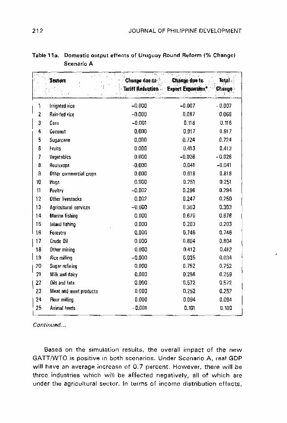
In *arms of specific industry effects, under Scenario A, three

industries will be negatively affected, all of which are from the

agricultural sector: irrigated rice, vegetables, and rootcrops (see Table

11a). Under manufacturing, the industry with the highest increase is

garments (5.8 percent), textile knitting (2.1 percent), other textiles

(1.9 percent), semi=conductor (1.1 percent), and other manufacturing

(1.0 percent). The rest of the industries have less than 1 percent

average increase. Under services, it will be government services

which will benefit the most, with an average increase of 2.3

percent per year.

Under Scenario B, 4 industries will be affected negatively. All of

the industries are in the agricultural sector. But the leading sectors

will be the government services with 0.151 percent increase.

Construction would increase by 0.07 percent, while [rode, storage

and warehousing will increase by 0.06 percent.


Table lOb, Impact on households:

average annual percentage, change over the lO-year period

Scenario B

,", '/f','l _' ' il,,,',,'Effect due All

.......... , ,:/, ,!':L!,,I,,,' to Export Shocks

: '/,f,i'!,' ' ', " ,,!, I !'i', '! ',Expansion*

Disposable income:

Household 1 0,000 0.251 0.251

Household 2 0,000 0.401 0.401

Household 3 0.O00 0.254 0.254

Household 4 0.000 0.218 0,218

Household 6 0.000 0.589 0.589

Labor Income of Households:

Household 1 0.000 0.490 0.490

Household 2 0.000 0.725 0.725

Household 3 0.000 0.435 0.435

Household 4 0.000 0.356 0.356

Household 5 0.000 0.928 0.928


SUMMARY

In terms of tariff change, the new GATT/WTO will not mean very

much as far as the Philippine industries are concerned. The present

tariff rates of almost all Philippine industries are below the initial

bound rate of the GATT/WTO set in 1995. Tariff protection in the

Philippines has declined considerably in the past years due to the

series of tariff reduction programs embarked on by the government to

liberalize the trade sector. However, the expected change in the world

economy in terms of trade expansion is significant as shown in the

different world growth scenarios presented in the paper. The paper

presented two scenarios of the world economy. Together with the

other changes, the paper simulated these to see the impact on the

local economy.

21 2 JOURNAL OF PHILIPPINE DEVELOPMENT

Table 11a. Domestic output effects of Uruguay Round Reform (% Change)Scenario A

1_: .... ............

L; TDt_I,=,, =,=....

.. " ,,,:: :,,: ' =,ii,/i!;i 'i. ,_', ,i:, ,, :_ =, ..........,r

1 Irrigatedrice -0.000 -0.007 -0.007

2 Rain-fedrice -0.000 0.067 0.066

3 Corn -0.001 0.118 0.116

4 Coconut 0.000 0.917 0.917

5 Sugarcane 0.000 0.724 0.724

6 Fruits 0.000 0.413 0.413

7 Vegetables 0.000 -0.026 -0.026

8 Roetcrops -0.000 -0.041 -0.041

9 Othercommercialcrops 0.000 0.818 0.818

10 Hogs 0.000 0.251 0.251

11 Poultry -0.002 0.296 0.294

12 Otherlivestocks 0.002 0.247 0.250

13 Agriculturalservices -0.000 0.303 0.303

14 Marinefishing 0.000 0_676 0.676

15 Inlandfishing 0.000 0.203 0.203

16 Forestry 0.0{30 0.746 {3.746

17 Crude0il 0.000 0.804 0.804

18 Othermining 0.000 0.412 0.412

19 Ricemilling -0.000 0.035 0.034

20 Sugarrefining 0.000 0.752 0.752

21 Milkanddairy 0.000 0.258 0.25922 0ilsendfats 0,000 (].572 0.572

23 Meatandmeatproducts 0.00g 0,252 0.252

24 Flourmilling 0.000 0_094 0.094

25 Animalfeeds -0.001 0.101 {3.100

Contmued..o

Based on the simulation results, the overall impact of the new

GATT/WTO is positive in both scenarios. Under Scenario A, real GDP

will have an average increase of 0.7 percent. However, there will be

three industries which will be affected negatively, all of which are

under the agricultural sector. In terms of income distribution effects,

CORORATON: SIMULATING THE EFFECTS OF GATT-UR/WTO 21 3

.,. con't, Table 11a

Sectors Changedueto Changedueto Total

Tariff Reduction ExportExpansion* Change

26 Otherfoods 0.000 0.420 0.420

27 Beverageandtobacco 0.000 0.374 0.374

28 Textilesknitting -0,000 2.073 2.073

29 Othertextiles 0.000 1.889 1.889

30 Garments,leatherandrubberfootwear 0.000 5.820 5.820

31 Woodproducts 0.000 0.699 0.700

32 Paperproducts 0.000 0,882 0.882

33 Fertilizer 0.000 0,532 0.532

34 Otlmrchemicals 0.030 0,758 0.758

35 Coalandpetroleum 0.000 0.848 0.84,8

36 Non-ferrousbasicmetals 0.000 0.735 8,735

37 Cement,basicmetalsandnon-metagic 0.000 0.577 0,578

38 Semi-conductor 0.000 1.130 1.130

39 Metalproductsandnon-electrical 0,000 0.481 0.482

40 Electricalmacbineries 0_0fig 0.359 0.359

41 Transportequipment 0.000 0.4,59 0.459

42 Miscellaneousmanufacturing -0.008 1.005 1,005

43 Construction 0.O00 0.344 0.344

44 Electricity,gasandwater 0.000 0.628 0,628

45 Transportandcommercialservices 0.000 0.696 0.696

46 Trade.storageandwarehousing 0.000 0,370 0.370

47 Banksandnon-hankservices 0.000 0.938 0,939

48 Insurances 0,000 0.873 0.874

49 GovernmentServices -0,001 2.285 2.285

50 OtherServices &BOO 0.464 0.465

with resource change

the results are mixed. In fact, the richest income group will benefit the

most, followed by the second household group.

Under Scenario B, real GDP will increase at an average of 0.64

percent, Manufacturing will be the leading sector. Mining industries

will be negatively affected, The effect on income distribution is

21 4 JOURNAL OF PHILIPPINE DEVELOPMENT

Tablellb. Domestic output effects of Uruguay Round Reform (% Change)Scenario B

, ' , i_,' ,, : , , : ,, _ ' ,..,

Sectors ",,!Changedue:ito Total

"','"Tariff,ReductiOn , ExportExpansion* Change' ' ' '":,, ',, ' ,, 'l',';" ' ' ' ' ' '

1 Irrigatec;rice -0,000 0,003 0.0032 Rain-fedrice -0.000 0.003 0.003

3 Corn -O.OOO -0.001 -0.001

4 Coconut -0.000 -0.002 -0.002

5 Sugarcane -0.OO0 0,001 0,0016 Fruits -0.000 -0.803 -0.003

7 Vegetables 0,000 0,002 0.002

8 Ro0tcrops ,-0.000 0.001 0,001

9 Othercommercialcrops 0.000 -0.000 -0.000

10 Hogs 0,000 0.003 0,003

11 Poultry -0.000 0,006 0,006

12 Otherlivestocks O,OOO &O04 0,004

13 Agriculturalservices -0.000 0,001 0.001

14 Marinefishing -0.O00 0,014 0.014

15 Inlandfishing -0,000 0.011 0.011

16 Forestry 0.000 0.012 O.Ol2

17 CrudeOil 0_000 0.000 0.060

18 Othermining 0.000 0,015 0,015

19 Ricemilling -0_000 0,008 0,008

20 Sugarrefining -0,000 0.001 0,001

21 Milkanddairy 0.000 0.001 0.001

22 0ilsandfats -0.000 0.002 0,002

23 Meatandmeatproducts 0.000 0.007 0,007

24 Flourmilling -0,000 0,001 0.001

25 Animalfeeds -0.000 0.001 0.001

Continued.,,

progressive. The poorest income groups will benefit the most. Under

this scenario, there will be 4 industries which will register negative

growth effect, These industries will come mostly from the agricultural

and mining sectors.

Although the overall simulated effects of the new GATT/WTO are

positive, they are just potential effects. They may not translate into

CORORATON: SIMULATING THE EFFECTS OF GATT-UR/WTO 21 5

... con't, Tzble 1lb

_ii$e_rJtts • ',',,,,,i ' Changedueto Total'

'! i,'i''_ ..... _ ; ," ExportExpansion* Change

26 Otherfoods -0.000 0.018 0,018

27 Beverageandtobacco 0,000 0,008 0.008

28 Textilesknitting -0.000 0.006 0.006

29 Othertextiles -0,000 0.002 0,002

30 Garments,leatherandrubberfootwear -0.000 0.020 0,020

31 Woodproducts 0.000 0,005 0.005

32 Paperproducts 0,000 0,009 0,009

33 Fertilizer 0,000 0.001 0,001

34 Otherchemicals -0.000 0.013 0,013

35 Coalandpetroleum 0,000 0.014 0.014

36 Non,ferrousbasicmetals -0,000 0.007 0.007

37 Cement,basicmetalsandnon-metallic 0,000 0.004 0,004

38 Semi-conductor -0,000 0,006 0.008

39 Metalproductsandnon-electrical =0.000 0,005 0.005

40 Electricalmachineries 0.000 0,002 0.002

41 Transportequipment 0.000 0,001 0.001

42 Miscellaneousmanufacturing 0.000 0,002 0.002

43 Construction 0,000 0.069 0.069

44 Electricity,gasandwater 0.000 0.016 0.016

45 Transportandcommercialservices 0,000 0,032 0,032

46 Trade,storageandwarehousing -0,000 0.060 0,06047 Banksandnon-bankservices 0,000 0,024 0.024

48 Insurances 0.000 0,053 0.053

49 GovernmentServices -0.000 0,151 0.151

50 OtherServices 0,000 0.038 0.038


higher growth (in particular higher export growth) in the localindustries unless other conditions are fulfilled. One such condition is

the improvement in the marketability of the country's product in the

international market. With the new GATT/WTO the world market will

be very competitive. Getting an additional market share in the world

market will be difficult. The task of getting additional market share in


the world market can probably be lightened if a concerted effort isexerted to address the problem of declining productivity in thePhilippine manufacturing sector. Cororaton et al (1995) found that inthe past three decades, productivity in the Philippine manufacturingsector dropped considerably. It was further established that the drop

was mainly caused by the absence of technical progress which, inturn, is related to outdated technology. Thus technology investmentand improvement in key strategic sectors of the economy will have tobe pushed and promoted. This can be done via transfer of technology

through direct foreign investment or joint ventures with foreign firms.These foreign firms will not only assist in terms of penetrating other

big markets where they are based, but they will also be the major thesource of new equipment and machineries and other information onefficient plant operations.

Another important factor to consider is an aggressive marketingeffort to penetrate markets especially in non-quota areas. Philippineexports go mainly to the US and Europe. With the gradual dismantlingof export quotas in these market under the new GATT/WTO, thePhilippines would have to penetrate quality-conscious markets suchas Japan. This is especially true for garments. Other markets in theArab countries will also be a promising market destination ofPhilippine exports.

CORORATON:SIMULATINGTHEEFFECTSOFGATT-UR/WTO 217

APPENDIX

THE APEX MODEL 4

There are a number of existing CGE models of the Philippine

economy. But the most recent and the biggest is the APEX model.APEX stands for agricultural policy experiments. Although the originalintention of the builders of the APEX model was to do policy

experiments for agriculture, at its present sectoral breakdown of 50sectors it can very well accommodate policy experiments for the other

two major sectors of the economy, the industrial and the servicesectors.

The entire agricultural sector is represented by 16 sectors in themodel; from rice (sections 1 and 2) to forestry (sector 16). The entireindustrial sector has 28 sub-sectoral breakdown, 24 of which are

manufacturing sectors, both food processing and non-foodmanufacturing. The other 4 sectors are mining and utilities sectors. Theservice sector is represented by 6 sectors in the model.

The APEX model is essentially a neoclassical, Walrasian, generalequilibrium model wherein the market clearing variables are prices. Themodel has well-defined production (or supply) and consumption (ordemand) sectors. These two major sectors are balanced through

changes in prices.The APEX model belongs to the Johansen (1962) class of applied

general equilibrium models 5 . The distinguishing characteristic of aJohansen-type model is that it is written as a system of linear equations

in percentage changes of the variables. 6 To see this clearly, assume a 2-sector model whose production can be written as

(1) Y = f(X 1, X2),

4. Thediscussionin this sectionis generallybasedon ClarateandWarr (1992). Foralengthyanddetaileddiscussionof the structureof the model,seathe referencecited.5. Another famousJohansen-typeCGEmodel is the Orani modelof the Australianeconomywhichis twice asbigas the APEXmodel.6. Fora detailedtreatmentof a 2-sectormodelseeDixon,at. al. (1982).

21 8 JOURNAL OF PHILIPPINEDEVELOPMENT

where Y is output and X 1 and X2 are inputs. In a Johansen-typemodel (1) is rewritten in linear percentage change form as

(2) y - elx 1 - e2x 2 = 0,

where e. is the elasticity of output with respect to inputs of factor i,I

and y, x 1 and x 2 are the percentage changes in Y, X 1, and X2.

In matrix notation, this type of model can be represented by

(3) Az = O,

where A is an (m x n) matrix of coefficients and z is an (n x 1)vector of percentage changes in the model's variables. Since the Amatrix is assumed fixed, (3) provides only a local representation of theequations suggested by economic theory, i.e., this equation is valid only

for "small" changes in X 1 and X 2.Through appropriate closure, z may be partitioned into a vector of

endogenous variables (y*) and a vector of exogenous variables (x*). 7Once the choice of exogenous variables has been made, (3) can berewritten as

(4) AlY* + A2x* = 0.

Provided A1 is invertible, one can proceed from (4) to the solution

" 1-1A2x*"(5) y -A

This equation expresses the percentage change in each endogenousvariable as a linear function of the percentage changes in the exogenousvariables.

The exogenous variables can be chosen in many different ways. Infact, much of the flexibility of the APEX model in policy applicationsarises from the user's ability to swap variables between the exogenousand endogenous categories.

To date, the APEX model is the most disaggregated applied generalequilibrium or computable general equilibrium model of the Philippineeconomy. On the production side, the model has 50 producer goods and

7. To solvethis model(n-m)variablemust bedeclaredexogenous.

CORORATON:SIMULATINGTHE EFFECTSOF GATT-UR/WTO 21 9

services sectors. On the demand side, the model has 7 categories ofconsumer goods and 5 household types.

The model is divided into agricultural and non-agricultural sectors.There are 3 primary factors which are mobile among the various non-agricultural industries. These are variable capital, skilled and unskilledlabor. Variable capital includes non-agricultural land and structureswhich are not necessarily devoted to any particular line of productionactivity, e.g. buildings and related fixed structures. Thus, when relativeprices change, owners of such land and capital assets can rent theseassets out to producers who face more favorable terms of trade.Unskilled labor is also freely mobile between non-agricultural andagricultural parts of the economy. However, skilled labor (defined toinclude high school graduates) and variable capital are not used inagriculture. Thus, skilled labor and variable capital are mobile onlyamong the non-agricultural industries of tile model.

There are 5 households classified as quintiles in the personalincome distribution. Each household is assumed to have its own

respective endowments in the primary factors in the model, i.e., eachhousehold derives its income from the sale of factor services and non-

factor income. The sources of household income include: labor income,

returns to variable and fixed capital, and rental income from letting outfarm lands in primary agricultural production. The household's non-factor income consists of lump sum net income transfers from thegovernment.

There are 7 consumer goods and services which are directly'7

consumed by the various households in the model. The consumedamounts of each of these consumer commodities and services are used

as arguments in the underlying utility functions of the various householdsof the model. Unlike producer goods, consumer goods production requiresonly intermediate goods as inputs, and not primary factors.

Household savings determine the total savings available forinvestment. The model assumes that only physical capital assets areobtainable using such savings. Financial assets such as bonds, equity,and bank deposits are not incorporated into the model. With this level ofsavings, additional units of physical capital are produced during thecurrent period. This capital is then allocated to each sector-specificcapital goods and the variable capital using the relative user cost ofsuch capital inputs.

An implicit financial assets market is assumed to exist wherebyevery household buys claims to every one of the fixed and variable


capital stock. Such claims entitle the household to a portion of thenewly produced capital during the current period. On the supply sideof such a market are the respective supplies Of fixed capital for eachof the 50 sector and the variable capital. Their respective entitlementsare then used to update the household's endowment in capital inputs,both fixed and variable.

Various industries of the model are classified as either export-oriented or import-competing. The criterion used for classifying theseindustries is the proportion of an industry's imports to its exports. If theratio exceeds 1.5 then the industry is regarded as producing animportable. The observed exports of this industry is regarded asexogenous in the model. However, if this ratio is less than 0.5, then theindustry is export-oriented. For ratios between 0.5 and 1.5, otherrelevant information was used in classifying the industry.

The APEX model assumes the country to be price taker in importedgoods. As in other CGE models, the APEX model imposes imperfect

substitutability between imports and locally produced products throughthe use of the Armington trade elasticities.

Export demand in the model have large but finite elasticities. Thecountry can be regarded as price taker in a particular commodity in theworld markets if the price elasticity of the world demand for the productis very large.

In the present model closure, the foreign exchange rate is assumedfixed. This therefore assumes that equilibrium in the external sector isreached through foreign capital flows. On the domestic side, equilibriumis reached through adjustments in the domestic absorption until savingsand government balances equate to zero. The model does this byintroducing a lump sum tax which assumes a positive (negative) valuewhenever the government incurs a deficit (surplus). This tax is capturedin the model by introducing a personal income tax rate shifter. Theshifter scales this rate up or down depending upon whether thegovernment is in deficit or surplus.

One important feature of the APEX model is that it uses empiricallyestimated behavioral parameters in its structure. Thus, essentiallyalmost all of the elasticities in the production, consumption, and tradesectors were estimated econometrically using Philippine data. 8

8. Fora detaileddiscussiononthe dataset usedto calibratethe modelseethe paperofClareteandCruz,1992.

CORORATON:SIMULATING THEEFFECTSOF GATT-UR/WTO 221

The benchmark period of the model is 1989. The major sources ofdata used to calibrate the model are: (i) 1985 input-output table. This

is used to specify the production side of the economy. The 1985 IOtable was updated to 1989 using the 1989 National Income Accountsof the Philippines; (ii) National Income Accounts for 1989; (3) 1991Philippine Statistical Yearbook; (4) 1988 Family Income andExpenditure Survey; (5) 1989 Foreign Trade Statistics of thePhilippines.


REFERENCES

Clarete, R. and Warr, P.G. "The Theoretical Structure of the APEX

Model of the Philippine Economy." 1992.Cororaton, C.; Endriga, B.; Ornedo, D.; Chua, C. 1995. "Estimation of

Total Factor Productivity of Philippine Manufacturing Industries: TheEstimates" Policy and Development Foundation, inc andDepartment of Science and Technolgy.

David, C. (1994) "GATT and Philippine Agriculture: Facts and Fallacies."Paper presented at the Symposium in Honor of Dr. Gelia Castillo,PSSC, Quezon City.

Francois, J., McDonald, B., and Norstom, H. 1993. "EconomywideEffects of the Uruguay Round" GATT Background Paper.

ILO-SEAPAT. 1995. "The Impact of GATT/URUGUAY Round on

Employment: Prospectd for the Philippines"Yang, Y. 1994 "Trade Liberalization With Externalities: A General

Equilibrium Assessment of the Uruguay Round" National Centre for

Development Studies, Australian National University

ping · Number 44, JournalVolume ofXXIVPhilippine, No. 2,DevelopmentSecond Semester 1997 ping...

Documents

Transcript of ping · Number 44, JournalVolume ofXXIVPhilippine, No. 2,DevelopmentSecond Semester 1997 ping...