PIG (SUS SCROFA) EXCLUSION IN MANOA WATERSHED … · i runoff, erosion, fecal indicator bacteria,...
136
I RUNOFF, EROSION, FECAL INDICATOR BACTERIA, AND EFFECTS OF FERAL PIG (SUS SCROFA) EXCLUSION IN MANOA WATERSHED A THESIS SUBMITTED TO THE GRADUATE DIVISION OF THE UNIVERSITY OF HAWAI‘I IN PARTIAL FULFILLMENT OF THE REQUIREMENTS FOR THE DEGREE OF MASTER OF SCIENCE IN NATURAL RESOURCES AND ENVIRONMENTAL MANAGEMENT (ECOLOGY, EVOLUTION, AND CONSERVATION BIOLOGY) DECEMBER 2009 By Dashiell O. Dunkell Thesis Committee: Gregory L. Bruland, Co-Chairperson Carl I. Evensen, Co-Chairperson Creighton M. Litton Mark Walker
Transcript of PIG (SUS SCROFA) EXCLUSION IN MANOA WATERSHED … · i runoff, erosion, fecal indicator bacteria,...
I
RUNOFF, EROSION, FECAL INDICATOR BACTERIA, AND EFFECTS OF FERAL
PIG (SUS SCROFA) EXCLUSION IN MANOA WATERSHED
A THESIS SUBMITTED TO THE GRADUATE DIVISION OF THE
UNIVERSITY OF HAWAI‘I IN PARTIAL FULFILLMENT OF THE
REQUIREMENTS FOR THE DEGREE OF
MASTER OF SCIENCE
IN
NATURAL RESOURCES AND ENVIRONMENTAL MANAGEMENT (ECOLOGY,
EVOLUTION, AND CONSERVATION BIOLOGY)
DECEMBER 2009
By
Dashiell O. Dunkell
Thesis Committee:
Gregory L. Bruland, Co-Chairperson
Carl I. Evensen, Co-Chairperson
Creighton M. Litton
Mark Walker

II
We certify that we have read this thesis and that, in our opinion, it is satisfactory in scope
and quality as a thesis for the degree of Master of Science in Natural Resources and
Environmental Management.
_____________________________
Co-Chairperson
_____________________________
Co-Chairperson
_____________________________
_____________________________

III
ACKNOWLEDGEMENTS
I greatly appreciate my advisors Dr. Greg Bruland and Dr. Carl Evensen, for the
guidance and assistance they have provided throughout my time at UH Manoa. I thank
my thesis committee members, Dr. Creighton Litton and Dr. Mark Walker for their
expertise and help with this project. I would like to thank Chad Browning, Ben Cooke,
Mark Chynoweth, Sarah Henly-Shepard, Safeeq Khan, Dereck Marciel, Leena Muller,
Emily Phares, Anne Quidez, Sarah Stebbing, and Adam Williams for assistance with
field and lab work. Thank you to Dr. Christopher Lepczyk for help with statistical
analyses. Thank you to Dr. Ali Fares for guidance and use of equipment.
Finally I would like to thank my family for all their love and support. I could
never have gotten this far without them.

IV
Abstract
While feral pigs (Sus scrofa) have impacted many ecosystems in Hawaii, their
effect on soil loss, water quality, and microbial contamination is not well known. This
study investigated the processes of runoff and soil erosion in upper forested areas of a
Hawaiian watershed and assessed the effects of feral pigs on erosion, runoff, water
quality, and pathogen transport. Runoff was collected monthly after storm events from
June 2008 to April 2009 at seven sites throughout Manoa watershed on the island of
Oahu. Each site consisted of paired runoff plots (5.04 m2) with one plot located inside a
fenced pig exclosure and the other located in the adjacent area subject to feral pig
activity. Forest composition and structure was measured at each site, including inventory
of all tree species, seedling and sapling counts, stand basal area, and stand density. Soil
moisture, throughfall, and runoff amount were recorded for each storm event. Runoff
volume was quantified and samples were tested for total suspended solids (TSS) and
Enterococcus spp. bacteria. Ground cover, infiltration, and Enterococci levels in soil
were also assessed. Runoff volumes varied from <1 to >128 L over the study period.
Repeated measures ANOVA indicated site by month and site by treatment (fenced versus
unfenced plots) interactions for runoff volume. Total SS levels in runoff ranged from
<0.01 to 7.05 g L-1. Repeated measures ANOVA indicated a site by month interaction for
TSS in runoff. While TSS levels were generally higher in wet season months, this was
not consistent across all sites. Enterococci in runoff ranged from <1 to 72,700 CFU 100
mL-1, and while the repeated measures ANOVA indicated a month by site interaction,
there were also significantly higher (α = 0.1) levels of from unfenced plots than fenced
plots. Enterococci in soil ranged from 24-476 CFU g-1, and differed significantly among

V
sites though not between fenced and unfenced treatments. According to multiple stepwise
regression, TSS in runoff was significantly related to throughfall, soil moisture, and
percent coarse woody debris cover, while Enterococci levels in runoff were significantly
related to runoff volume.

VI
Table of Contents Acknowledgements………………………………………………………………………III
Abstract………………………………………………………………………………..…IV
List of Tables…………………………………………………………………………..VIII
List of Figures…………………………………………………………………………….X
List of Abbreviations……………………………………………………………………XII
Chapter 1: Introduction and Background……………………………………………….…1
1.1 Introduction…………………………………………………………………………..1
1.2 Hawaiian Watersheds, Runoff, and Sediment Transport…………………………….2
1.3 Infiltration, Permeability and Throughfall…………………………………………...4
1.4 Fecal Indicator Bacteria……………………………………………………………...5
1.5 Feral Pigs and Invasive Species……………………………………………………...7
1.6 Study Area: Manoa Watershed……………………………………………………..11
1.7 Research Objectives………………………………………………………………...16
Chapter 2: Sediment in Runoff…………………………………………………………..19
2.1 Introduction…………………………………………………………………………19
2.2 Site Selection……………………………………………………………………….20
2.3 Site Layout………………………………………………………………………….22
2.4 Runoff Plot Design…………………………………………………………………23
2.5 Activation Periods and Runoff Sampling…………………………………………..26
2.6 Estimation of Other Environmental Variables……………………………………...27
2.7 Runoff Collection and Analysis…………………………………………………….32
2.8 Statistical Analysis………………………………………………………………….34
2.9 Soils………………………………………………………………………………...34
2.10 Throughfall………………………………………………………………………..37
2.11 Infiltration…………………………………………………………………………38
2.12 Species, Stem Density, and Basal Areas of the Study Sites………………………39
2.13 Ground Cover……………………………………………………………………..43
2.14 Runoff Volume……………………………………………………………………49

VII
2.15 Total Suspended Solids in Runoff……………………………………………..….54
2.16 Correlation of TSS with Environmental Variables………………………………..57
2.17 Discussion…………………………………………………………………………60
2.18 Conclusions………………………………………………………………………..69
Chapter 3: Enterococci in Runoff and Soils……………………………………………..72
3.1 Introduction…………………………………………………………………………72
3.2 Site Selection……………………………………………………………………….73
3.3 Site Layout………………………………………………………………………….76
3.4 Runoff Plot Design…………………………………………………………………77
3.5 Activation Periods and Runoff Sampling…………………………………………..78
3.6 Estimation of Other Environmental Variables……………………………………..79
3.7 Runoff Collection and Analysis…………………………………………………….84
3.8 Enterococci in Soils...………………………………….…………………………...87
3.9 Statistical Analyses…………………………………………………………………87
3.10 Enterococci in Runoff.…………………………………………………………….88
3.11 Enterococci in Soils...……………………………………………………………..92
3.12 Correlation of Enterococci with Environmental Variables………………..………94
3.13 Discussion…………………………...…………………………………………….97
3.14 Conclusions………………………………………………………………………103
Chapter 4: Conclusions…………………………………………………………………107
4.1 Further Research…………………………………………………………………..109
4.2 Recommendations for Improvement………………………………………………110
Appendix A……………………………………………………………………………..112
Appendix B……………………………………………………………………………..114
Appendix C……………………………………………………………………………..117
Literature Cited…………………………………………………………………………121

VIII
List of Tables Table Page
2.1. Characteristics of seven sites in Manoa watershed…………………...…………….22
2.2. ANOVA for mean soil moisture……………………………………………………35
2.3. ANOVA for throughfall means………..………………………………………...…38
2.4. Saturated hydraulic conductivity (Ksat) across plots………………………………39
2.5. Stem density and basal area for the seven sites…………………………………….40
2.6. List of canopy tree species observed at the seven sites……..……………………...41
2.7. List of mid-story woody plant species observed at the seven sites…………………41
2.8. ANOVA for ground cover fenced versus unfenced means among sites……..…….45
2.9. ANOVA for bare soil fenced versus unfenced means among sites………..……….48
2.10. ANOVA for runoff amount means………………………………………………..51
2.11. ANOVA for TSS means…………………………………………………………..55
2.12. Spearman correlation matrix for the environmental variables and TSS…………..60
3.1. Characteristics of seven sites in Manoa watershed………………………….…..….76
3.2. ANOVA overall model for Enterococci levels in runoff…………………….……..88
3.3. ANOVA for site effects on Enterococci levels in soil…………....………………...91
3.4. ANOVA for treatment effects on Enterococci levels in soil……..………………...91
3.5. Spearman correlation values for Enterococci and environmental variables.….…....95
4. List of canopy tree species at Lyon Arboretum……………………………………..111
5. List of canopy tree species at Manoa Cliffs…………………………………………111
6. List of canopy tree species at Manoa Falls………………………………………….111
7. List of canopy tree species at Pauoa Flats…………………………………………..112
8. List of canopy tree species at Puu Pia……………………………………………….112
9. List of canopy tree species at Roundtop…………………………………………….112
10. List of canopy tree species at Roundtop…………………………………………...112

IX
List of Figures Figure Page
1.1. Manoa Stream Network…………………………………………………………….13
1.2. GIS map of land use in the Manoa watershed……………………………………...14
1.3. GIS map with locations of 8 sites……….……..…………………………………...15
2.1. GIS map of slope with locations of 8 sites…………………….…….……………..21
2.2. Site layout…………………………………………………………………………..23
2.3. Photo of runoff plot at Roundtop site………………………………………………25
2.4. Location of seedling and sapling counts……………………………………………30
2.5. Ground cover transects……………………………………………………………..32
2.6. Average soil moisture per month prior to rain event………………..……………..35
2.7. Average soil moisture per site prior to rain event………………………………….36
2.8. Average soil moisture per plot prior to rain event………………………………….36
2.9. Average throughfall of rain events per month..……………………………………37
2.10. Average throughfall of rain events per site……………………………………….38
2.11. Seedling occurrence per site………………………………………………………42
2.12. Sapling occurrence per site………………………………………………………..42
2.13. P. cattleianum seedling and sapling occurrence…………………………………..43
2.14. Ground cover in fenced versus unfenced runoff plots, averaged among sites…….45
2.15. Photograph of Waahila Ridge site………………………………………………...46
2.16. Ground cover at Waahila Ridge, fenced versus unfenced runoff plots…………...46
2.17. Bare soil ground cover, runoff plots, fenced versus unfenced treatment…………47
2.18. Ground cover at Roundtop, fenced versus unfenced runoff plots…………...........48
2.19. Whole plot ground cover, fenced versus unfenced, average among all sites……..49
2.20. Average runoff volume in liters per rain event among months...…………………51
2.21. Average runoff volume in liters, among sites………………………... …………..52
2.22. Average runoff volume in liters, among all plots…………………………………52
2.23. Runoff volume sums from collection buckets and overflow buckets……………..53
2.24. Average TSS per month …………………………………………………………..55

X
2.25. Average TSS per site………..……………………….……………………………56
2.26. Average TSS per month fenced vs. unfenced treatment………………….……….56
2.27. Average TSS per plot……………………………………………………………..57
2.28. Isohyetal rainfall pattern and location of sites in Manoa Watershed……………...63
2.29. Rainfall per month from USGS Kanewai Field rain gauge……………………….63
2.30. Game camera photo of feral pig at Manoa Cliffs…………………………………64
3.1. GIS map of Manoa watershed and locations of 8 study sites………………………75
3.2. Site layout…………………………………………………………………………..77
3.3. Location of seedling and sapling plots at each site…………………………………83
3.4. Location of ground cover transects…………………………………………………84
3.5. Average Enterococci levels in runoff among months……………..…………....…..89
3.6. Average Enterococci levels in runoff among sites…………...……………...….….90
3.7. Average Enterococci levels in runoff between treatments…………………………90
3.8. Average Enterococci levels in soils among sites……………………… …………..92
3.9. Average Enterococci levels in soils between treatments……………………….......92
4. Lyon Arboretum ground cover……………………………………………………...113
5. Manoa Cliffs ground cover………………………………………………………….113
6. Manoa Falls ground cover…………………………………………………………..114
7. Pauoa Flats ground cover………………………………………………………...….114
8. Puu Pia ground cover……………………………………………………………..…115

XI
List of Abbreviations
ANOVA analysis of variance BA basal area CFU colony-forming units CV coefficient of variation CWD coarse woody debris DBH diameter at breast height DI de-ionized GIS geographic information system GLM general linear model GPS global positioning system HVNP Hawaii Volcanoes National Park Ksat saturated hydraulic conductivity LYF Lyon (fenced) LYU Lyon (unfenced) MCF Manoa Cliffs (fenced) MCU Manoa Cliffs (unfenced) MFF Manoa Falls (fenced) MFU Manoa Falls (unfenced) MRG Manoa Rain Gauge MSR multiple stepwise regression NRCS Natural Resources Conservation Service PFF Pauoa Flats (fenced site) PFU Pauoa Flats (unfenced site) PPF Puu Pia (fenced site) PPF Puu Pia (unfenced site) rRT Rough Mountainous Land RTF Round Top (fenced site) RTR runoff-throughfall ratio RTU Round Top (unfenced site) TSS total suspended solids USGS United States Geological Survey WRF Waahila Ridge (fenced site) WRU Waahila Ridge (unfenced site)

1
CHAPTER 1: INTRODUCTION AND BACKGROUND
1.1 Introduction
Many watersheds on the island of Oahu are characterized by small drainage
basins, primarily trade-wind driven precipitation, and steep, forested headwaters. These
upper forested areas are often important conservation lands that, amongst other things,
supply irrigation and drinking water to many Hawaii residents. The Manoa watershed on
Oahu contains both high mountainous and low-level coastal lands within a relatively
small area. While precipitation and stream-flow data from Manoa Valley have been
recorded for many years, there remain many unanswered questions about throughfall and
runoff dynamics in the watershed. Even less is known about the watershed-scale effects
of nonnative feral pigs (Sus scrofa) on processes such as erosion, runoff, and pathogen
generation.
In Hawaii, feral pigs have invaded many ecosystems and their effect on water
quality and microbial contamination is not well understood. Of the hundreds of invasive
species in Hawai‘i, the feral pig has arguably caused the most damage, especially in wet
forests (Tomich, 1979). Pig activities such as rooting, browsing, digging, and trampling
may lead to a loss of biodiversity, propagation of invasive plants, and increased erosion
(Hone and Stone, 1990; Huenneke and Vitousek, 1990; USGS, 2006). As a result of these
activities, feral pigs in Hawaii are considered by many to be a threat to native flora and
fauna, and minimizing their impact is a top priority for many of Hawaii’s parks and
reserves (Hone and Stone, 1989; Huenneke and Vitousek, 1990).
The objectives of this study were to improve our understanding of the processes

2
of runoff and soil erosion in upper forested areas of a Hawaiian watershed, and to identify
the effects pigs have on erosion, runoff, water quality, and pathogen transport. It has been
hypothesized that feral pigs not only harm native flora and fauna, but may even adversely
impact the health and function of entire watersheds (Noguiera-Filho et al., 2009). Such
effects raise important concerns for public health. It is, therefore, imperative to
investigate how feral pigs influence runoff, soil loss, and bacteria levels to develop
appropriate and effective management practices. The data collected from this project will
be of interest to managers, the public, and policy makers. Runoff dynamics in upper
forested watersheds in Hawaii are not well understood, and while there is much suspicion
about negative impacts of feral pigs on the ecology and function of these areas, there is
little hard evidence.
1.2 Hawaiian Watersheds, Runoff, and Sediment Transport
Tropical volcanic island ecosystems, such as the Hawaiian Archipelago, are
subject to high erosion and sedimentation hazards and, therefore, are extremely sensitive
to the impacts of land use and management (El-Swaify, 2000). Native Hawaiians
developed a land management system called the ahupua’a, which was similar to the
modern term ‘watershed’ but also integrated the coastline and inshore and offshore ocean
waters. Headwater areas in Hawaii are often located in high-rainfall forested mountains,
many of which are conservation areas. The two principal sources of surface water in
Hawaiian watersheds are overland runoff following rainfall and groundwater discharge.
Overland runoff is typically episodic and varies widely in intensity depending on the type
of rain. The volume of direct surface runoff depends on the intensity and persistence of

3
the rain, as well as the size, geology, and morphology of the drainage basin. Previous
research has indicated that forested basins in the Koolau Mountain range on Oahu yield a
surface runoff volume equal to about 35% of the rainfall of a moderate to heavy
rainstorm (Lau and Mink, 2006).
According to Lau and Mink (2006) the only extant observed data of overland flow
water quality in forested areas were obtained for a small area in the drainage basin of
Aihualama Stream, a tributary of Manoa Stream. The results from 17 rainfall episodes
between September 1974 and March 1975 indicated high organic loads with minimal
biodegradation in the fast-moving water. The high total solids were largely suspended
(81%). The direct overland flow contained high levels of heavy metals, and would have
failed to meet current stream water quality standards. The response of runoff to rainfall
on annual and regional bases in Hawaii is usually described as a simple linear equation,
RO = a' + b'P, where a' and b' are constants, and P is precipitation (Lau and Mink, 2006).
A different correlation for central and southern Oahu gives direct runoff as RO =
0.0021P2 (Lau and Mink, 2006).
It is widely accepted that vegetative cover can reduce overland flow, and this has
been clearly demonstrated in Hawaiian agricultural soils (Ryder and Fares, 2008). Other
permeable Hawaiian soils, even though bare, can absorb high amounts of rainwater
before overland flow occurs. Initiation of overland flow on bare soils was investigated
with simulated rain in ten different soils series from the Islands of Hawaii and Oahu (Lau
and Mink, 2006). Results showed that runoff initiation time varies linearly with
antecedent saturation deficit. For wet soil with a deficit of less than 5%, the initiation
times were just a few minutes. However, in some cases initiation times were greater than

4
80 minutes. These long times suggest runoff generated by saturation from below the soil
layers, rather than limitation by the infiltration capacity of the soils.
Although surface erosion is a natural process, it is exacerbated by surface
disturbance and compaction that reduce soil hydraulic conductivity and break down soil
aggregates (Sidle et al. 2006). Historically, soil erosion has been a problem in Hawaii at
least since the introduction of exotic ungulates soon after European contact (El-Swaify,
2000; Nogueira-Filho et al., 2009). Sediment transport to a stream depends on numerous
factors which vary with respect to climate, vegetation cover, and soil type (Lai and
Detphachanh, 2006). Sedimentation has multiple negative impacts that affect watersheds
and adjacent coastal areas. These include nutrient influx carried by sediments; damage
caused to streams, estuaries, and coral reefs from increased turbidity; and the cost of
dredging coastal waterways. Given these impacts it is important to quantify runoff and
sediment dynamics in the watersheds of Hawaii. It is also important to understand how
feral pigs contribute to erosion, runoff, and pathogen transport to best identify and
implement proper watershed-based management strategies.
1.3 Infiltration, Permeability and Throughfall
Infiltration is the process by which water enters the ground surface. Infiltration
rate depends on soil texture and compaction, initial soil water content, vegetation cover,
and rate of water application. Initial water intake may exceed water application rate until
ponding occurs. Infiltration capacity denotes the maximum rate that occurs under the
ponding conditions. Various studies of Hawaiian soils recorded values from 0.3 to greater
than 6.0 m d-1 of infiltration (Lau and Mink, 2006). Values between 0.3 and 1.2 m d-1 are

5
reported for forest sites near Lyon Arboretum (Lau and Mink, 2006).
Studies have shown the reduction of infiltration as the result of various land uses
(Lau and Mink, 2006; Ryder and Fares, 2008). Cultivated lands have infiltration rates
four times less than adjacent forest lands (Lau and Mink, 2006). Urban lands have
reported losses of infiltration capacity as high as 83%. Hydraulic conductivity, K, is a
measure of the permeability of soil or rock. Permeability of soils is affected by soil
structure, porosity, and texture. Saturated hydraulic conductivity (Ksat) values of
Hawaiian soils are typically a few meters per day, though Ksat can be reduced by 50%
during wet soil conditions (Lau and Mink, 2006).
In most forests, the infiltration capacity and hydraulic conductivity of surface
soils are relatively high (Sidle et al., 2006). High infiltration capacities are supported by
continual inputs of organic matter onto the soil surface. Because tropical forest soils
experience high rates of decomposition, organic horizons are typically thin compared to
temperate soils (Lau and Mink, 2006). In undisturbed forests, precipitation generally
infiltrates into the soil and moves to streams as subsurface flow. Exceptions may occur in
steep slopes or sites with a low permeability layer near the surface that promotes return
flow during storms with wet antecedent conditions. However, many tropical soils exhibit
marked decreases in hydraulic conductivity in the upper portion of the soil profile and
still transmit most water to streams via subsurface flow.
1.4 Fecal Indicator Bacteria
Indicator organisms (IOs) are commonly used to quantify fecal contamination of
water bodies, and are an integral part of water management plans (Plummer and Long,

6
2007). Indictor organisms reside in the gastrointestinal tracts of humans and animals, and
are used throughout the world to assess the microbiological safety of drinking,
recreational, and shellfish waters. They are found in fecal material at high concentrations
and are easier to measure in the environment than are pathogens. Although IOs do not
cause illness under normal conditions, they represent a measure of fecal contamination.
The great diversity of pathogenic microorganisms transmitted by contaminated water and
the difficulty and cost of directly measuring all microbial pathogens in environmental
samples leads to the use of indicator organisms that may indicate the presence of sewage
and fecal contamination (Gersberg et al., 2006; Wade et al., 2006). The U.S.
Environmental Protection Agency recommends the use of Escherichia coli, a member of
the fecal coliform group, as an IO for recreational waters in freshwater bodies and
members of the genus Enterococcus (the Enterococci) for both freshwater and saltwater
(Anderson et al., 2005).
This study employs Enterococcus spp. bacteria as an IO to investigate water
quality of runoff in the Manoa watershed. Enterococci abundance is one of the three most
common water quality tests in the United States (Noblea et al., 2003). From Santa
Monica Bay, California to the Great Lakes, levels of indicator bacteria have been shown
to correlate well with incidence of illness reported by swimmers (Haile et al., 1999;
Wade, 2006). Though some research suggests that Enterococci are free-living in
Hawaiian soils (Hardina and Fujioka, 1991), mesocosm experiments have found that
Enterococci do not multiply in subtropical waters and sediments (Anderson et al., 2005).
Recent unpublished data from remote, undisturbed locations on Oahu revealed extremely
low Enterococci levels in surface waters (Ragosta, 2007).

7
A study in Massachusetts showed the highest IO densities occurred during spring
and summer, and the lowest densities during the fall and winter (Plummer and Long,
2007). However, this result was likely caused by the presence of housing complexes in
the study area, which seemed to leach consistent amounts of waste throughout the year.
Therefore human contamination was greater in dryer months when there was less dilution
from rain and surface flow. Another study in California found that feral pigs preferred
riparian areas during the summer months (Cushman et al., 2004).
1.5 Feral Pigs and Invasive Species
1.5.1 Feral Pigs in Hawaii
Feral pigs, descended from wild boars native to North Africa and parts of Eurasia,
are now found in a diverse range of habitats on all continents except Antarctica, as well
as many oceanic islands (Ickes et al., 2001). Early Polynesian settlers first introduced
Polynesian pigs to the Hawaiian Islands as an important food source (Katahira et al.,
1993). Later Captain Cook brought European pigs during his first voyage to Hawaii.
Many other introductions followed, and pigs became feral and dispersed throughout all
the major Islands. Now the only main Hawaiian Islands free of feral pigs are Lanai and
Kahoolawe (Noguiera et al., 2007).
1.5.2 Health Risks
Feral pigs can harbor and spread many potential human pathogens. It should be
noted that most pathogens are not solely spread by feral pigs. Other warm-blooded
mammals such as the mongoose and rat also likely play a role in their distribution. There
are many possible human health risks caused by feral pig activities in watersheds. For

8
example, studies of feral pigs in Australia have shown that the foraging and wallowing
behavior of pigs can markedly increase the turbidity of water supplies, and more
importantly, they can transmit and excrete a number of infectious waterborne organisms
pathogenic to humans (Hampton et al., 2006). Specifically, populations of feral pigs may
serve as an environmental reservoir of Cryptosporidium parvum oocysts and Giardia spp.
cysts for source water (Atwill et al., 1997). Other important protozoan parasite pathogens,
such as Balantidium, and Entamoeba, were detected from the feces of feral pigs caught in
metropolitan drinking water catchments (Hampton et al., 2006). All are potentially
important waterborne human pathogens that pose a threat to water quality.
1.5.3 Pig Behavior
Pigs consume and trample understory plants, disperse plant propagules, degrade
native bird habitat by disturbing the understory and influencing forest succession,
produce breeding sites for mosquitoes, and disrupt nutrient cycling (Katahira et al., 1993,
Nogueira et al., 2007). Pigs are omnivorous and have even been shown to threaten
endangered shorebirds through predation of eggs (Donlan et al., 2007). Pig foraging
activities are known to have impacts on soil erosion, soil horizon mixing, nutrient
leaching, and litter layers (Spear and Chown, 2009). These activities can also decrease
biodiversity and increase soil bulk density. Foraging can cause introduction of exotic
species, especially strawberry guava (Psidium cattleianum) which is invading many
forests throughout Hawaii. Feral pigs spread P. cattleianum seeds through feces, and their
rooting behavior causes disturbances that may enhance its spread (Huenneke and
Vitousek, 1990).
Feral pig’s effects on ecosystems may often be attributed to rooting behavior

9
(Noguiera-Filho et al., 2009). Pigs frequently feed on plants and invertebrates in the soil.
A large amount of digging and/or rooting is required for pigs to access these food
sources. Digging generally refers to the pig’s browsing activity when searching for soil
invertebrates (often earthworms). Rooting occurs when pigs remove roots of typically
younger plants. Anderson et al. (2007) reported that a single pig could physically disturb
200 m2 of rain forest surface in one day. Rooting is commonly used as an indicator of pig
population density (Hone, 1988). In a related measure, the amount of exposed soil in a
forested system may be an indicator of the rooting intensity of the site (Campbell and
Long, 2009). Pig rooting has been shown to accelerate nutrient leaching, increase soil
erosion, limit soil regenerating processes, and reduce soil arthropods (Campbell and
Long, 2009).
Pig rooting was found to be more frequent in upper elevations and drainage lines
in watersheds in Australia (Hone, 2002). In Hawaii Volcanoes National Park (HVNP),
rooting behavior caused 70% of fresh and intermediate disturbance along pig activity
transects (Katahira et al., 1993). Pig activity in the 5 x 10 m plots ranged from 0.1-3.6 %,
with a mean of 0.7 %. Estimated pig density ranged from 0.8- 4.7 pigs km-2, with a mean
of 0.8 pigs km-2. Pig activity and density in all three units combined had a statistically
significant linear relationship. In Australia feral pig disturbance was found to be most
common on flat slopes at high elevations, and least common on steep slopes at low
elevations (Hone, 1995).
Hone and Stone (1989) found foraging and trampling by pigs can cause severe
erosion and may lead to the degradation of watersheds. This can be especially harmful in
watersheds such as Manoa because pigs typically inhabit areas of steep terrain (Hone and

10
Stone, 1989). Pigs also inhibit watershed function by increasing runoff through the
compaction of soils. Wallowing, creation of pig trails, and the crushing of vegetation to
browse for food and creation of nests all contribute to soil compaction. In a study at
HVNP, Vtorov (1993) found total density of microarthropods in soils nearly doubled and
biomass increased 2.5 times, seven years after exclusion of feral pigs. These native
microarthropods are indicators of soil quality and important contributors to the soil
formation process. In sites with pigs, disturbance to litter and compaction of the upper
soil horizons created a substrate relatively unsuitable for microarthropod populations.
Soil density around tree ferns, a favorite food of feral pigs, was 30% higher than
surrounding areas (Vtorov, 1993).
1.5.4 Invasive Species
Introduction of invasive species is of great concern all over the world, but
especially for island ecosystems (Donlan and Wilcox, 2008). Invasive species are one of
the main reasons Hawaii is home to 31% of the species on the U.S. endangered species
list (Allison and Miller, 2000). Hundreds of exotic species are problematic invaders in
Hawaii, and feral pigs are considered one of the worst (Nogueira et al., 2007). Indigenous
forests on oceanic islands such as New Zealand and the Hawaiian Islands have evolved in
isolation from major landmasses and in the absence of mammalian herbivores. As a
result, indigenous flora in such areas exhibit a high degree of endemism and are often
vulnerable to damage from mammalian herbivory (Sweetapple and Nugent, 2004).
Nonnative ungulates carry out novel functions in systems devoid of indigenous large
herbivores through herbivory and by increasing soil nitrogen (Spear and Chown, 2009).
Introduced ungulates may also alter fire or erosion regimes (Spear and Chown, 2009).

11
Biological invasions are a global phenomenon that can alter disturbance regimes
and facilitate colonization by other nonnative species (Cushman et al., 2004). A study of
a California grassland found that feral pigs promoted the colonization of nonnative grass
and forb species (Cushman et al., 2004). Introduced ungulates also have the potential to
change the rate and trajectory of recovery of patches of forest that have been damaged by
natural and human-induced disturbances (Wilson et al., 2006). In the presence of
ungulates, vegetation will often reestablish on these patches more slowly and with a
different species composition than in the absence of ungulates (Wilson et al., 2006).
In Hawaiian rain forests, an unharvested pig population is potentially capable of
doubling every four months (Katahira et al., 1993). Except for malnutrition, disease, or
cold weather during farrowing at high elevations, there are no other known natural factors
limiting pig populations in Hawaii (Katahira et al., 1993). Feral pigs, through a
combination of herbivory, predation, competition, and habitat effects, are considered a
threat to biodiversity in the U.S., and seem to be a species of particular concern globally
(Spear and Chown, 2009). Impacts of nonnative mammals on plant regeneration and
other processes are fairly well known, however watershed-scale effects of feral pigs have
rarely been studied in the Pacific Islands, and peer-reviewed research is scarce.
1.6 Study Area: Manoa Watershed
The Manoa Valley watershed is the ideal place for this study for many reasons.
Foremost, the University of Hawaii Manoa is situated such that evaluation and analysis of
samples are relatively fast and straightforward. Likewise, the timely sampling of streams
and runoff plots are expedited when rain events do occur. Manoa Valley is diverse in

12
terrain, relief, and rainfall, as well as land use and vegetation types. Feral pigs are the
only large non-human mammal that occurs in the study area, unlike many of the other
Pacific Islands where deer (Axis axis, Odocoileus hemionus), cattle (Bos taurus) and
goats (Capra aegagrus) can occupy the same habitat as pigs.
Manoa watershed encompasses approximately 2,528 ha in southeast Oahu. It
contains both high mountainous and low-level coastal lands within a relatively small
area. Runoff from Manoa watershed is carried by two main streams, Manoa and Palolo
Streams, which join each other before emptying into the Ala Wai Canal (Fig. 1.1).
Historically, the area surrounding the Ala Wai Canal, as well as all of Waikiki, formed a
much larger coastal wetland and the streams of Manoa and Palolo flowed into this area
separate from one another. Construction of the Ala Wai Canal was completed in 1928.
The canal performed its intended function of draining the surrounding wetlands,
including agricultural lands, to allow for further development (Glenn and McMurtry,
1995). However, since its construction issues such as dredging, water quality, and flood
control have posed numerous concerns to local residents, engineers and lawmakers.
13
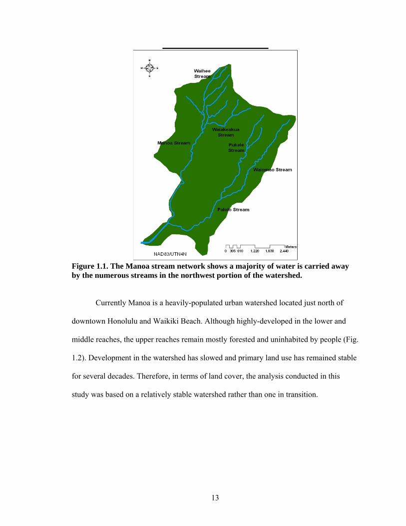
Figure 1.1. The Manoa stream network shows a majority of water is carried away by the numerous streams in the northwest portion of the watershed.
Currently Manoa is a heavily-populated urban watershed located just north of
downtown Honolulu and Waikiki Beach. Although highly-developed in the lower and
middle reaches, the upper reaches remain mostly forested and uninhabited by people (Fig.
1.2). Development in the watershed has slowed and primary land use has remained stable
for several decades. Therefore, in terms of land cover, the analysis conducted in this
study was based on a relatively stable watershed rather than one in transition.

14
Figure 1.2. A GIS map of land use in the Manoa watershed.
The previous installation of runoff plots in the study area provided a unique
opportunity for further study (Browning, 2008). The location of plots allowed for in
relief, dominant vegetation, and rainfall. The upper part of the watershed is characterized
by steep terrain, higher rainfall rates, and is dominated in places by strawberry guava
(Psidium cattleianum) and bamboo (Poaceae spp.). The lower part of the watershed has
flatter terrain and lower rainfall. Runoff plots are situated in areas with varying slope,
rainfall, and vegetation cover (Fig. 1.3).

15
Figure 1.3. GIS map of Manoa Watershed slope with streams, trails, and the eight runoff plot sites.
The presence of pigs in the Manoa watershed is a divisive issue in the surrounding
community, and among the many stakeholders who use the area. The pigs are hunted for
their meat and for recreation, so a sustainable population is seen as a positive to some
local people. However, many scientists, environmentalists, and local residents are
concerned about the potential damage pigs may cause to the native vegetation and
riparian areas. There are also concerns about the disturbance and danger of hunting the
pigs and the use of hunting dogs. The possible threat to human health is an important
concern, and the many recreational users of the Manoa Valley should be informed of the
risks. There is anecdotal evidence that pig populations are increasing, and that pigs are
interacting with humans more often. Pig threats to human health may also be increasing

16
and the need to study this issue is urgent.
Feral pigs have been shown to have negative effects on soil properties as well as
ecosystem functions and biodiversity (Hone, 2002), but no one has ever investigated any
link to fecal contamination in runoff to pigs in Manoa Valley or in other tropical island
watersheds. In Hawaii, the streams and downstream coastal water are highly prized for
recreation, and tourists visit from all over the world to enjoy the abundant natural
resources. Any possible threat to public health or environmental quality should be
researched.
Manoa Valley has a high annual rainfall, and one study in Hawaii found an
exponential increase in feral pigs relating to antecedent rainfall (Caley, 1993). Visual
assessment and eyewitness reports have suggested a large pig population living in the
Manoa watershed. Reports in the local media have suggested that feral pig interactions in
urban areas are increasing as well, worrying homeowners and public health authorities
(Nogueira et al., 2007). The data collected from this project will be of interest to
managers, the public, and policy makers. The results and recommendations of this
research may lead to reduced soil erosion, mitigation of stream degradation, and
improved health of estuarine and coral reef ecosystems.
1.7 Research Objectives
The overall objective of this thesis is to investigate runoff processes that occur in
the forested upper areas of Manoa watershed and to examine the use of exclusion fencing
as a tool to improve water quality. The specific objectives are as follows: (1) Quantify
throughfall, runoff amount, total suspended solids (TSS) in runoff, and Enterococci in

17
runoff and soils from forested areas of Manoa watershed; (2) Determine if feral pigs
impact runoff amount, TSS in runoff, and Enterococci in runoff and soils; (3) Investigate
temporal and spatial differences in TSS and Enterococci levels in runoff; and (4)
Investigate correlations among environmental variables (slope, infiltration rate, soil
moisture, stem density, etc) and TSS and Enterococci in runoff. Given what was learned
in the literature review, and drawing on the results of previous research at these sites
(Browning, 2008), I developed four hypotheses:
Hypotheses:
(1) Higher storm intensity and higher throughfall inputs will lead to larger runoff
amounts, and higher TSS and Enterococci levels in runoff during the wet season
(November-April) than in the dry season (May-October);
(2) Fecal contamination will lead to higher Enterococci levels in runoff and soil at
unfenced plots exposed to feral pig activity;
(3) Of all environmental predictors measured, ground cover and soil moisture will
have the strongest correlations with TSS and Enterococci in runoff as ground
cover influences soil erosion processes, and Enterococci survival is thought to be
higher and infiltration is lower under wetter soil conditions which directly affect
runoff production;
(4) TSS in runoff will positively correlate with Enterococci abundance in runoff
as bacteria are thought to associate with soil particles in surface waters.

18
The hypotheses listed above address a gap in our knowledge as to the contribution
of sediments from forested and upper watershed areas in Hawaii, and the effects of feral
pigs on runoff and soil loss. Runoff plots have often been employed in agricultural
settings in Hawaii (El-Swaify, 1989; Ryder and Fares, 2008) but this is one of the first
times they have been used in upper forested watershed areas (Browning, 2008). While
feral pig impacts have been theorized and visual evidence is plentiful, few attempts to
quantify the actual amount of runoff/soil loss exist, particularly in Hawaiian watersheds.
Fecal contamination caused by pigs has rarely been studied in the Pacific Islands, and
never in Manoa. This study will aid natural resource managers, helping them identify the
effects of feral pigs, and informing them of the effectiveness of fencing as a tool for
increasing water quality. This information will also allow landowners to protect the
health of riparian areas, and could benefit swimmers and other recreational users of
Hawaiian streams and rivers.

19
CHAPTER 2: SEDIMENT IN RUNOFF 2.1 Introduction
This study aims to improve our understanding of the processes of runoff and soil
erosion in upper forested areas of a typical Hawaiian watershed and to identify the effects
pigs have on erosion and runoff. Feral pigs can harm native flora and fauna, and may
even adversely impact the health and function of entire watersheds (Noguiera-Filho et al.,
2009). Runoff dynamics in upper forested watersheds are not well understood, and while
there is much suspicion about negative impacts of feral pigs on ecology of these areas
there is little hard evidence. Sedimentation has multiple negative impacts that affect
watersheds and adjacent coastal areas; including nutrient influx carried by sediments,
damage caused to streams, estuaries, and coral reefs from increased turbidity, and the cost
of dredging coastal waterways. Given these impacts it is important to quantify runoff and
sediment dynamics in the watersheds of Hawaii. It is also important to understand how
feral pigs contribute to erosion and runoff in order to best identify and implement
appropriate watershed-based management strategies.
The specific objectives of this chapter are to: (1) quantify throughfall, runoff
amount, and total suspended solids (TSS) in runoff from selected forested areas of Manoa
watershed; (2) determine if feral pigs increase runoff amount and TSS in runoff; (3)
examine temporal and spatial differences in TSS levels in runoff; and (4) investigate
correlations among environmental variables (slope, infiltration rate, soil moisture, stem
density, etc) and TSS. The specific hypotheses tested are as follows: (1) Higher storm
intensity and higher throughfall inputs will lead to larger runoff amounts, and higher TSS

20
levels in runoff during the wet season (November-April) than in the dry season (May-
October); (2) pig disturbance will lead to higher TSS levels in runoff at unfenced plots
exposed to feral pig activity; (3) of all environmental predictors measured, ground cover
and soil moisture will have strongest correlations with TSS in runoff, as ground cover
influences soil erosion processes and infiltration is lower under wetter soil conditions
which directly affect runoff production.
Materials and Methods
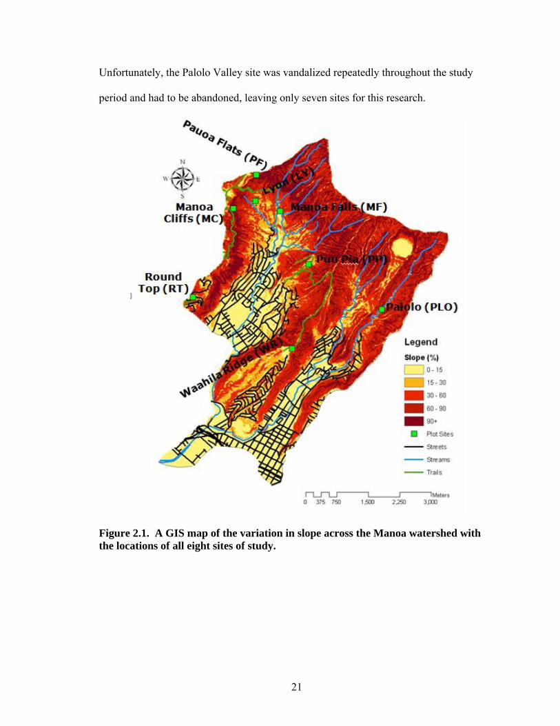
2.2 Site Selection
In the spring of 2007, eight sites were selected to investigate runoff processes and
the effects of feral pig exclusion in Manoa watershed. The sites were chosen from the
upper forested areas of the watershed, based on attributes of slope, accessibility, and
vegetation. Slope was the primary determining factor in initial site selection to allow for
construction of exclusion fencing and to ensure collection of accurate runoff data.
According to Mutchler et al. (1994) a slope of 9% or less is considered the standard in
most agricultural studies that incorporate runoff plots; however areas with <9% slope
were not easy to find as the average slope of the watershed is 47%. Using a Geographic
Information System (GIS), a map of slope characteristics throughout the watershed was
created and areas with slopes between 5-30% were identified as potential sites (Fig. 2.1).
Final site selection was based on ease of accessibility and proximity to existing trail
networks as well as homogeneity of slope/vegetation at each site (Table 2.1).
21
Unfortunately, the Palolo Valley site was vandalized repeatedly throughout the study
period and had to be abandoned, leaving only seven sites for this research.
Figure 2.1. A GIS map of the variation in slope across the Manoa watershed with the locations of all eight sites of study.

22
Table 2.1. Characteristics of seven sites in Manoa watershed. Elevation and soil series information was obtained through a GIS analysis, while slopes were recorded on site using a handheld clinometer. Site Elevation (m) Slope (%) Soil Series
Lyon 215 15.5 Lolekaa
Manoa Cliffs 450 8 Rough Mountainous Land
Manoa Falls 171 17 Lolekaa
Pauoa Flats 538 6 Rough Mountainous Land
Puu Pia 209 26 Lolekaa
Round Top 340 25.5 Tantalus
Waahila Ridge 340 14 Manana
2.3 Site Layout
Each site is approximately 10 x 10 m. Two paired 10 m by 5 m runoff plots were
established at each site; one runoff plot surrounded by exclusion fencing, the other
unexclosed. Runoff plots were oriented down the slope to effectively capture the natural
path of overland flow at each site. Fences were constructed of 14-gauge utility fencing
0.91 m tall and held in place with metal posts. Barbed wire was strung along the bottom
edge of each fence to provide further protection from pig damage. During initial
construction of runoff plots, throughfall gauges were affixed to posts directly centered
between the paired plots at each site. In December 2008, four additional throughfall
gauges were added to each site (Figure 2.2).

23
Figure 2.2. The layout of each of the 7 sites. Each site was oriented so both fenced and unfenced plots had similar slope and vegetation.
2.4 Runoff Plot Design
Following fence installation, runoff plots were constructed within both unfenced
and fenced plots at each site. Runoff plots were approximately 4.2 m long by 1.2 m wide,
oriented down the prevailing slope. To prevent additional runoff entering from outside
the plot, 15 cm tall plastic dividers were buried roughly 7.5 cm into the soil along the
upslope and outer edges of each runoff plot. These plastic pieces formed the framework
that channeled runoff to a central collector (Fig. 2.3). This central collector was located at
the down slope end of the runoff plot, consisting of a triangular metal runoff collector
that funneled all runoff into a 10 by 5 cm opening (Fig. 2.3). A metal feed tray connected
the metal collector to an 18.9 L bucket for storing runoff. A rectangular hole was cut into
the side of the bucket into which the feed tray drained. Water-tight lids were affixed to

24
the top of each bucket to prevent throughfall from falling directly into the bucket. Sheet
metal collector covers were constructed to also prevent direct throughfall on the metal
collector and installed in December 2008.

25
Figure 2.3. A photo from the Round Top site displaying the runoff collection system.

26
2.5 Activation Periods and Runoff Sampling
Runoff samples were collected from June 2008 to April 2009 to ensure collection
of samples from both the wet and dry seasons. At the beginning of each month a two-day
dry period was targeted to activate all plots and initiate runoff collection. Activation of
each site included emptying all throughfall gauges, collecting soil samples for moisture
analysis, and emptying/cleaning the runoff collection buckets. Runoff was removed with
a hand operated suction pump, and then paper towels were used to clean and dry all
inside surfaces of collection buckets. Sterile latex gloves were worn at all times during
emptying and cleaning procedures. Collection times were determined by observing
weather conditions and monitoring the online USGS rain gauge located in Manoa Valley.
When the rain gauge recorded a significant rainfall (typically > 2 cm) during the active
period, collection was initiated.
The collection process involved measurement of total runoff and collection of
runoff sub-samples to be analyzed for TSS. During all activation and collection
activities, care was taken to avoid walking within runoff plots. Soil samples were taken
within the sites, yet outside the runoff plots so as not to disturb soils. In the duration
between observation periods runoff was allowed to continue its natural flow into the
buckets. If the buckets began to overflow, runoff simply drained out through the same
opening from which it entered and continued flowing down slope. Throughfall gauges
were covered with duct tape while not active.

27
2.6 Estimation of Other Environmental Variables
As this project was designed to monitor runoff and sediment loss from the study
areas and to develop correlation and regression equations for TSS in runoff, it was
important to quantify a variety of different variables that influence these processes. This
required recording of site characteristics throughout the duration of the study, as well as
prior to rain events, and also the analysis of runoff after the events. The other
environmental variables recorded were slope, soil series, soil water content, throughfall,
infiltration rate, forest canopy and understory species composition, stem density, basal
area of trees, seedling/sapling counts, and ground cover assessment. The following
paragraphs summarize the methodology used to determine these characteristics.
2.6.1 Slope Recordings
Slopes were measured using a handheld clinometer and ranged from 5% to 27%.
No site was recorded to have greater than a 2% difference between the fenced and
unfenced plots. Ultimately, all seven sites represented a range of different slope types as
shown in Table 2.1.
2.6.2 Soil Series Determination
Soil series for each site were obtained from digital NRCS soil maps. Additionally,
global positioning system (GPS) coordinates for each site recorded in the field. These two
data layers were overlaid to identify the soil series of each site based on the latest soil
survey of Oahu (Foote et al. 1965). The seven sites represented four different soil series;
Tantalus, Lolekaa, Manana, and Rough Mountainous Land (rRT) (Table 2.1).

28
2.6.3 Calculation of Soil Water Content
Gravimetric soil water content was determined during the activation phase of each
month. A 2 cm diameter soil corer was used to collect samples from approximately the
upper 5 cm of the soil profile. One composite sample was collected during site activation
from both the fenced and unfenced areas. The composite sample consisted of three
separate randomly-located individual samples from each area, combined in a sterile
plastic bag. No soil samples were taken from within runoff plots to avoid disturbing soils.
Percent gravimetric soil moisture was calculated by the equation:
% Gravimetric Soil moisture = ( 1 - (dry mass soil / wet mass soil) ) x 100
2.6.4 Throughfall Recording
A standard all-weather rain gauge (Productive Alternatives, Fergus Falls, MN)
was used to measure throughfall (mm) of rain events. As part of the activation process,
each throughfall gauge was emptied and a thin layer of vegetable oil was added to
prevent evaporation.
2.6.5. Infiltration Rates
Infiltration rate and the coefficient of saturation (Ksat) were determined at each
plot using a Tension Infiltrometer (8 cm model, Soil Measurement Systems, Tucson,
AZ). The most level and uniform area of each fenced/unfenced plot (although not within
the runoff plot areas) was chosen as the infiltration measurement site. A metal spatula
was used to cut out a shallow hole in the litter layer the same size/shape as the

29
infiltrometer base to expose the soil surface. A layer of fine sand was added to the hole.
The infiltrometer was then filled with water and placed on the sand layer. The tension
was set to 11 cm. If infiltration did not commence, tension was lowered to 10 cm.
Readings of water level were taken every 30 seconds for 10 minutes, then every 60
seconds for another 10 minutes, and a final reading was taken after five more minutes.
The tension was then lowered to 8 cm if initial tension was 11 cm, or 7.5 cm if initial
tension was 10 cm. This was to ensure enough of a tension difference between the two
readings to allow for calculation of Ksat.
Equilibrium infiltration slopes were determined graphically. The slope was then
multiplied by the area of the infiltrometer’s base to determine the volume of water
infiltrated per time. Ksat was calculated from the equation:
α = LN (Infiltration rate X / Infiltration rate Y) (- Tension X - Tension Y)
Ksat = Infiltration rate X Area of base ^ (α * Tension X) * (1 + 4 / Area of base * α)
Where X = tension 1, and Y = tension 2
2.6.6 Forest Structure Characterization
The seven sites in Manoa Valley varied in terms of forest structure and species
composition. To quantify these differences, a 20 m by 20 m plot directly surrounding
each site was established and all trees > 2 cm diameter at breast height (DBH) were
measured. DBH is defined as diameter at 1.32 m from the ground surface. Species was
recorded for each tree in the plot. If a tree could not be identified to the species level in

30
the field, a leaf sample was taken back to the lab for identification. Stem density (# stems
ha-1) was calculated by counting the number of stems in the 400 m2 plot and scaling to a
hectare basis. Basal area (m2 ha-1) of each tree was calculated from individual DBH
measurements, and summed to give total basal area in the 400 m2 plot, which was scaled
to a hectare basis.
2.6.7 Seedling and Sapling Counts
Seedlings and saplings were measured in two 1 m2 plots within each fenced and
unfenced plot (Figure 2.4). Measurements were taken at the upper and lower outside
corner (the only corners without rain gauges) of each plot. This was done to minimize
any effects of trampling or disturbance from previous research activities in the plots (e.g.
throughfall gauge sampling). Seedlings were defined as any plant < 15 cm in height.
Saplings were defined as all plants > 15 cm in height, but less than 2 cm DBH. Species
identification was determined in the field or with voucher specimens.
Figure 2.4. Location of seedling and sapling plots at each site.

31
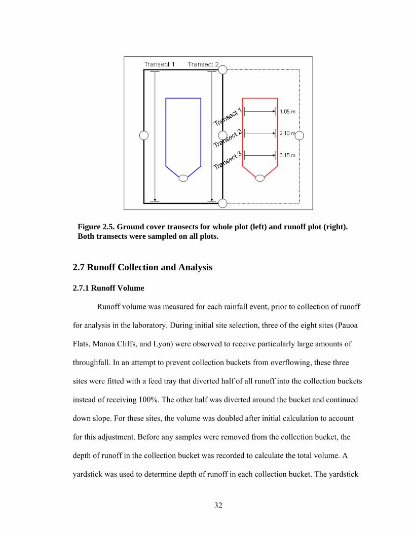
2.6.8 Estimation of Ground Cover
Ground cover at the sites was recorded for both the runoff plots and the larger
fenced/unfenced area. A measuring tape was used to establish a transect line and a visual
assessment of ground cover was made at predetermined distances along the transects. For
the whole plot, measurements were taken every 25 cm along two separate 10 m transects
(Figure 2.5). Ground cover measurements in the runoff plot were taken every 3 cm along
three 1.2 m transects equally spaced along the runoff plot. Visual determination of
ground cover was made from a direct top-down view above the transects. Ground cover
was divided into the following categories: live plant, standing dead plant, coarse woody
debris, litter, bare soil, rock, and root. Coarse woody debris was defined as woody
debris/branches > 2 cm diameter. Litter included detritus, leaves, and any woody debris <
2 cm diameter.
32
2.7 Runoff Collection and Analysis
2.7.1 Runoff Volume
Runoff volume was measured for each rainfall event, prior to collection of runoff
for analysis in the laboratory. During initial site selection, three of the eight sites (Pauoa
Flats, Manoa Cliffs, and Lyon) were observed to receive particularly large amounts of
throughfall. In an attempt to prevent collection buckets from overflowing, these three
sites were fitted with a feed tray that diverted half of all runoff into the collection buckets
instead of receiving 100%. The other half was diverted around the bucket and continued
down slope. For these sites, the volume was doubled after initial calculation to account
for this adjustment. Before any samples were removed from the collection bucket, the
depth of runoff in the collection bucket was recorded to calculate the total volume. A
yardstick was used to determine depth of runoff in each collection bucket. The yardstick
Figure 2.5. Ground cover transects for whole plot (left) and runoff plot (right). Both transects were sampled on all plots.

33
was cleaned with paper towels after each use. Sterile latex gloves were worn at all times,
and changed prior to each new measurement.
2.7.2 Runoff Overflow Buckets
During the initial months of this study, it was recognized that runoff collection
buckets were in many cases too small to collect the total amount of runoff from certain
rainfall events. A small hole was drilled in the downslope edge of each collection bucket
and a length of rubber hose was inserted in the hole. The rubber hose was layed
downslope and inserted into another hole drilled into a larger plastic tub (the “overflow
bucket”). This overflow bucket captured extra runoff to a volume of 97.7 L. A yard stick
was used to record runoff overflow volume as above.
2.7.3 Quantification of Total Suspended Solids in Runoff
After the depth was recorded, the contents of the collection bucket were
thoroughly mixed with the yardstick and a runoff water sample was collected in an acid-
washed 500 mL bottle. Samples were taken back to the lab on ice and refrigerated before
analysis for total suspended solids (TSS). Total SS were measured by vacuum filtration
of 100 mL of sample. First a Whatman 5 filter paper (Whatman, Kent, United Kingdom)
was placed on a watch glass and weighed on an electronic balance. Samples were
homogenized and a 100 mL aliquot was extracted and poured onto filter paper placed on
a Buchner funnel attached to a 500 mL vacuum flask. Each filter paper and watch glass
were then placed into a 105oC oven and dried for 24 hours. Afterwards the filters were

34
weighed and the original weight was subtracted from the dry weight to calculate the TSS
in g L-1 (EPA, 1971).
2.8 Statistical Analyses
All statistical analyses were performed using SAS version 9.1 (SAS Institute,
Cary, NC). A Repeated Measures ANOVA (Proc MIXED) was used to distinguish
differences between fenced and unfenced treatments, among months, and among sites.
Month was the repeated measure in these analyses. Proc MIXED uses the ‘containment
method’ and, depending on the homogeneity of variances, denominator degrees of
freedom may vary from one model to another. Post hoc comparisons of means were
conducted with least squares method. A Linear Model GLM ANOVA was used to
distinguish differences between treatments and among sites for environmental variables
that were only measured once. In these cases, a one-way ANOVA was used to make a
distinction between ground cover in fenced and unfenced sites and post-hoc comparisons
of means were carried out using the Duncan’s Multiple Range Test. A Spearman
correlation was used to evaluate associations among TSS and all environmental variables.
A multiple stepwise regression (MSR) was also used to determine the best predictors of
TSS in runoff.
Results
2.9 Soils

35
Soil moisture was significantly different among months and sites, though there
was also a significant site by month interaction (Table 2.2). April had the highest mean
soil moisture, which was significantly higher than November, December, and February;
but not January or March (Figure 2.6). These mean differences highlighted a trend of
wetter soils as the wet season progressed.
0%
10%
20%
30%
40%
50%
60%
November December January February March April
Gra
vim
etri
c S
oil
Mo
istu
re
Table 2.2. Repeated Measures ANOVA for soil moisture Source
Num df
Den df
Chi- Square
F-statistic
p-value
Site 5 30 32.21 6.44 0.0004 Month 6 6 165.71 27.62 0.0004 Treatment 1 6 0.05 0.05 0.83 Month x Site 30 30 73.38 2.45 0.0084 Month x Treatment 5 30 2.86 0.57 0.72
On average, across the study period, gravimetric soil moisture was significantly
higher at Manoa Cliffs (64.1%) than any other site (Figure 2.7). Roundtop (33.1%) had
significantly lower soil moisture than any site except Waahila Ridge (38.5%). Waahila
Figure 2.6. Mean soil moisture per month prior to rain events. Error bars represent ± 1 standard error. Letters represent differences according to least squared means.
AB B AB B AB
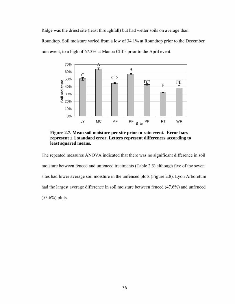
36
Ridge was the driest site (least throughfall) but had wetter soils on average than
Roundtop. Soil moisture varied from a low of 34.1% at Roundtop prior to the December
rain event, to a high of 67.3% at Manoa Cliffs prior to the April event.
0%
10%
20%
30%
40%
50%
60%
70%
LY MC MF PF PP RT WRSite
So
il M
ois
ture
The repeated measures ANOVA indicated that there was no significant difference in soil
moisture between fenced and unfenced treatments (Table 2.3) although five of the seven
sites had lower average soil moisture in the unfenced plots (Figure 2.8). Lyon Arboretum
had the largest average difference in soil moisture between fenced (47.6%) and unfenced
(53.6%) plots.
Figure 2.7. Mean soil moisture per site prior to rain event. Error bars represent ± 1 standard error. Letters represent differences according to least squared means.
A
CCD
DEF
B
FE

37
0%
10%
20%
30%
40%
50%
60%
70%
LY MC MF PF PP RT WRSite
So
il M
ois
ture
Fenced
Unfenced
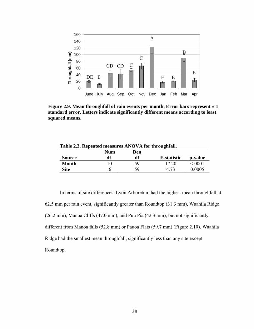
2.10 Throughfall
Throughfall amounts were significantly different among months and among sites
(Table 2.3). The site by month interaction could not be tested because of a lack of
replication of throughfall measurements at the sites. Throughfall per rain event varied
from a mean of 11.6 mm in July to 122.3 mm in December (Figure 2.9). The December
event was significantly greater than all other months. March had the next highest
throughfall (89.6 mm), and was also significantly different from all other months.
January was the next smallest event after July; averaging 17.2 mm. February was the
fourth-smallest event, 20.0 mm, averaging less than 1 mm more than June (19.2 mm).
From July through December average throughfall increased steadily, then after December
average throughfall decreased. The dry season months of June and July were not
significantly different from the wet season months of January, February and April (Table
2.3).
Figure 2.8. Mean soil moisture per plot prior to rain events. Error bars represent ± 1 standard error.
38
0
20
40
60
80
100
120
140
160
June July Aug Sep Oct Nov Dec Jan Feb Mar Apr
Th
rou
gh
fall
(mm
)
Table 2.3. Repeated measures ANOVA for throughfall. Source
Num df
Den df
F-statistic
p-value
Month 10 59 17.20 <.0001 Site 6 59 4.73 0.0005
In terms of site differences, Lyon Arboretum had the highest mean throughfall at
62.5 mm per rain event, significantly greater than Roundtop (31.3 mm), Waahila Ridge
(26.2 mm), Manoa Cliffs (47.0 mm), and Puu Pia (42.3 mm), but not significantly
different from Manoa falls (52.8 mm) or Pauoa Flats (59.7 mm) (Figure 2.10). Waahila
Ridge had the smallest mean throughfall, significantly less than any site except
Roundtop.
Figure 2.9. Mean throughfall of rain events per month. Error bars represent ± 1 standard error. Letters indicate significantly different means according to least squared means.
A
C
CDCD
B
C
DE E
E EE

39
0
10
20
30
40
50
60
70
80
90
LY MC MF PF PP RT WRSite
Th
rou
gh
fall
(c
m)
2.11 Infiltration
Infiltration rates and saturated hydraulic conductivity (Ksat) varied greatly among
sites and between fenced and unfenced plots (Table 2.4). There was a difference of four
orders of magnitude between the largest and smallest Ksat values. Even between fenced
and unfenced plots there were huge differences in Ksat. The Waahila Ridge fenced plot
had a Ksat that was ~1,400 times greater than the Ksat in the unfenced plot. The Puu Pia
unfenced plot had the highest Ksat of 723 m hr-1, while the Waahila Ridge unfenced plot
had the lowest with <0.01 m hr-1.
Site - Plot Ksat (m hr-1) Lyon Arboretum - Fenced 21.75 Lyon Arboretum - Unfenced 0.055 Manoa Cliffs - Fenced 0.21 Manoa Cliffs - Unfenced 0.48 Manoa Falls - Fenced 1.41 Manoa Falls - Unfenced 91.08
Figure 2.10. Mean throughfall of rain events per site. Error bars represent ± 1 standard error. Letters indicate significantly different means according to Duncan’s Multiple Range test.
Table 2.4. Saturated hydraulic conductivity (Ksat) values (m hr-1) across all sites and plots.
A AB
AB
BC BC
BCD D

40
Pauoa Flats - Fenced 0.096 Pauoa Flats - Unfenced 0.83 Puu Pia - Fenced 0.17 Puu Pia - Unfenced 723.11 Roundtop - Fenced 54.21 Roundtop - Unfenced 17.00 Waahila Ridge - Fenced 103.83 Waahila Ridge - Unfenced 0.007
2.12 Species, Stem Density, and Basal Areas of the Study Sites
Stem density ranged from less than 1,500 stems hectare-1 (ha) at Pauoa Flats,
dominated by large Elaecarpus grandis (blue marble) trees, to more than 9,000 stems ha-1
at Puu Pia (Table 2.5). Basal area ranged from just over 20 m2 ha-1 to >132 m2 ha-1.
Psidium cattleianum (strawberry guava) tended to form dense monocultures of small
trees, particularly at Manoa Falls and Waahila Ridge, contributing to the high stem
densities at these sites. Schefflera actinophylla (octopus tree) also formed dense stands,
though with larger average DBH than P. cattleianum, at Puu Pia and Roundtop.
Site Stem Density (stems ha-1)
Basal Area (m2 ha-1)
Lyon Arboretum 1,900 41.0 Manoa Cliffs 3,375 20.0 Manoa Falls 5,175 74.0 Pauoa Flats 1,475 37.7 Puu Pia 9,300 132.7 Roundtop 2,400 93.8 Waahila Ridge 4,625 47.6
A total of 14 different canopy tree species were observed at the seven sites (Table
2.6). Each site also had a different mix of species (Appendix A). Another five woody
plant species were found in the mid-story range (Table 2.7) and Ardisia crenata (Hilo
Table 2.5. Stem density and basal area for the seven sites.

41
holly) was measured only as a seedling or sapling. Ardisia elliptica (shoebutton ardisia)
was the most common species, found at six of seven sites, though typically in individuals
<2.0 cm DBH.
Table 2.6. List of canopy tree species observed at the seven sites. Species Name Common Name Casaurina glauca Ironwood Cinnamomum burmanni padang cassia Elaecarpus grandis blue marble Eucalyptus robusta swamp mahogany Ficus microcarpa Chinese banyan Hibiscus tiliaceus Hau Hibiscus arnottianus kokio keokeo Persea americana Avocado Pisonia umbellifera pepala kepau Psidium cattleianum strawberry guava Psidium guajava common guava Schefflera actinophylla octopus tree Unknown #2 Unknown #3 Unknown #7 Unknown #8
Table 2.7. List of mid-story woody plant species observed at the seven sites. Species Name Common Name Ardisia elliptica shoebutton ardisia Dracaena sp. money tree Cestrum nocturnum night-blooming jasmine Cordyline terminalis ti or ki Livistona chinensis Chinese fan palm
Seedling and sapling counts revealed differences from the canopy composition
(Figures 2.11, 2.12). Mid-story species, especially A. elliptica, appeared in high numbers
in sapling and seedling counts. Two sites, Waahila Ridge and Roundtop, contained no
seedlings or saplings. Waahila Ridge was dominated by Causarina glauca (ironwood)

42
trees in a monotypic stand directly over the runoff plots, and the thick litter layer appears
to prevent other species from establishing there. Within the larger 400 m2 area there was
also a dense stand of P. cattleianum trees, as mentioned above, but none of these trees
were within either the fenced or unfenced plot.
At the Manoa Cliffs fenced plot, seedling counts of Cinnamomum burmannii were
greater than 70 individuals m-2. This area was dominated in places by thick C. burmannii
canopy that shades out most other plants. Other understory plants observed at Manoa
Cliffs were Hedychium sp. (ginger) and Cestrum nocturnum (night-blooming jasmine).
Pauoa Flats was another site with high counts of C. burmannii, averaging almost 23
seedlings m-2. The understory at Pauoa Flats also included large numbers of A. elliptica,
more than 10 seedlings m-2.
LYF
LYU
MC
F
MC
U
MF
F
MF
U
PF
F
PF
U
PP
F
PP
U
RT
F
RT
U
WR
F
WR
U
0
2040
60
80
100
120
140
160Ardisia crenata
Ardisia elliptica
Cinnamomum burmanii
Cestrum nocturnum
Psidium cattleianum
Figure 2.11. Seedling occurrence across the fenced and unfenced plots of each site.
43
LYF
LYU
MC
F
MC
U
MF
F
MF
U
PF
F
PF
U
PP
F
PP
U
RT
F
RT
U
WR
F
WR
U
0
2
4
6
8
10
12
14
Ardesia crenata
Ardesia elliptica
Cinnamomum sp.
Cestrum nocturnum
P. cattleianum
Schefflera actinophylla
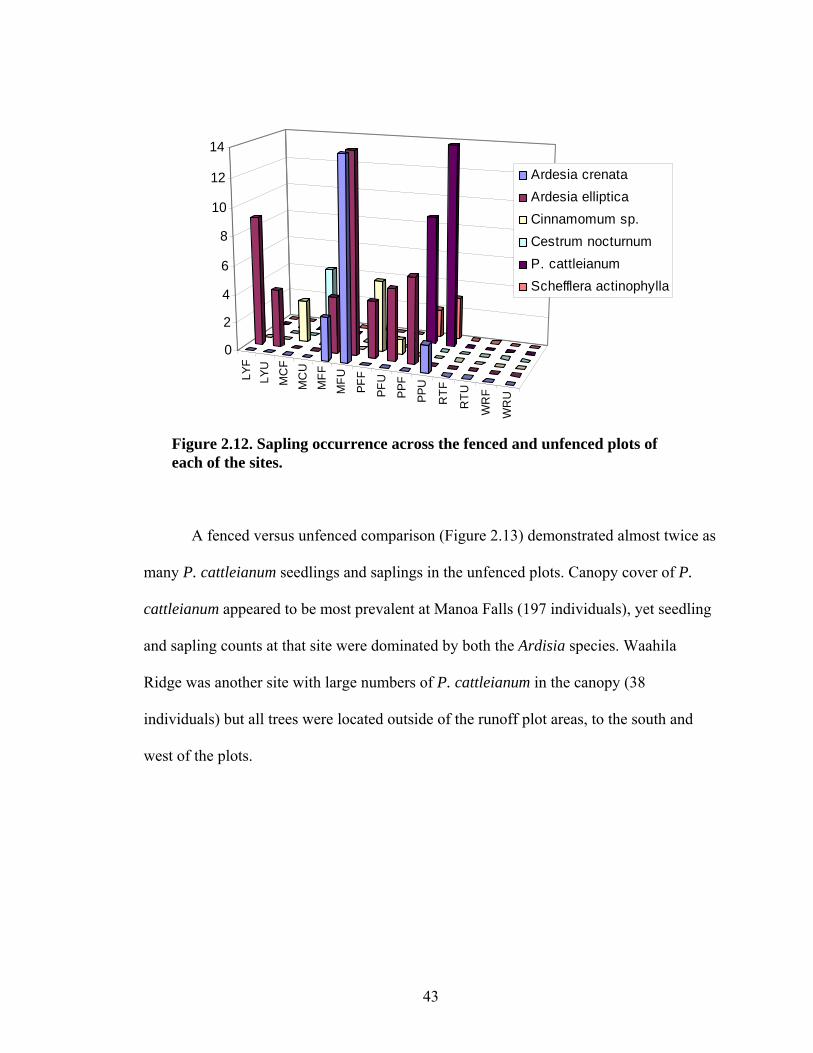
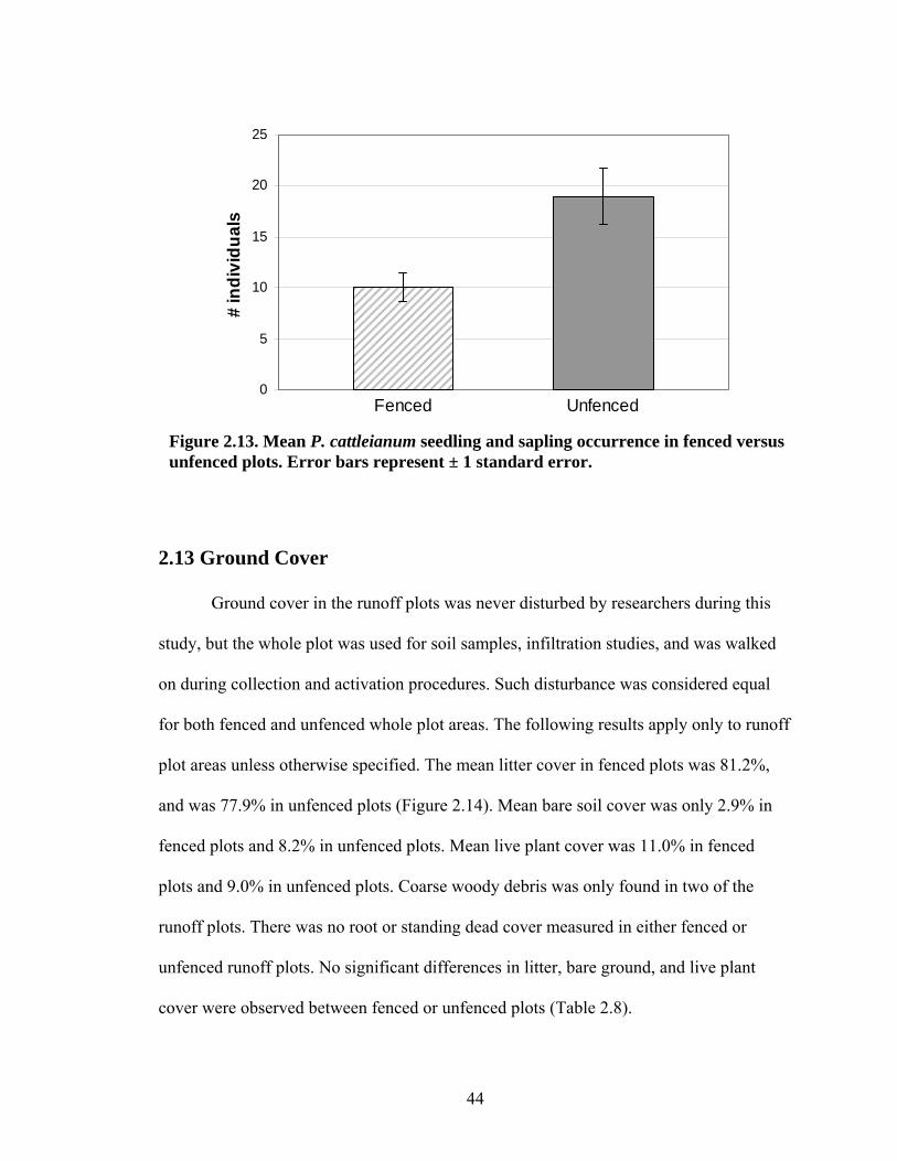
A fenced versus unfenced comparison (Figure 2.13) demonstrated almost twice as
many P. cattleianum seedlings and saplings in the unfenced plots. Canopy cover of P.
cattleianum appeared to be most prevalent at Manoa Falls (197 individuals), yet seedling
and sapling counts at that site were dominated by both the Ardisia species. Waahila
Ridge was another site with large numbers of P. cattleianum in the canopy (38
individuals) but all trees were located outside of the runoff plot areas, to the south and
west of the plots.
Figure 2.12. Sapling occurrence across the fenced and unfenced plots of each of the sites.
44
Fenced Unfenced0
5
10
15
20
25
# in
div
idu
als
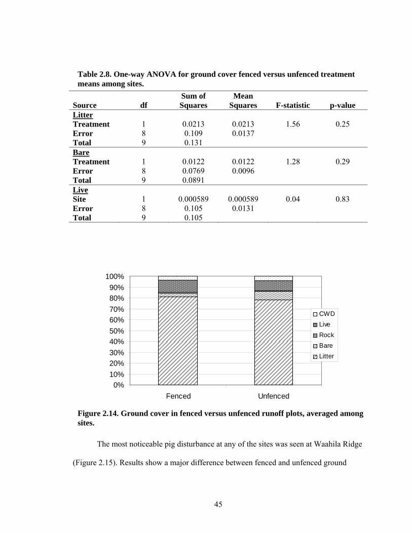
2.13 Ground Cover
Ground cover in the runoff plots was never disturbed by researchers during this
study, but the whole plot was used for soil samples, infiltration studies, and was walked
on during collection and activation procedures. Such disturbance was considered equal
for both fenced and unfenced whole plot areas. The following results apply only to runoff
plot areas unless otherwise specified. The mean litter cover in fenced plots was 81.2%,
and was 77.9% in unfenced plots (Figure 2.14). Mean bare soil cover was only 2.9% in
fenced plots and 8.2% in unfenced plots. Mean live plant cover was 11.0% in fenced
plots and 9.0% in unfenced plots. Coarse woody debris was only found in two of the
runoff plots. There was no root or standing dead cover measured in either fenced or
unfenced runoff plots. No significant differences in litter, bare ground, and live plant
cover were observed between fenced or unfenced plots (Table 2.8).
Figure 2.13. Mean P. cattleianum seedling and sapling occurrence in fenced versus unfenced plots. Error bars represent ± 1 standard error.
45
Source df Sum of Squares
Mean Squares F-statistic p-value
Litter Treatment 1 0.0213 0.0213 1.56 0.25 Error 8 0.109 0.0137 Total 9 0.131 Bare Treatment 1 0.0122 0.0122 1.28 0.29 Error 8 0.0769 0.0096 Total 9 0.0891 Live Site 1 0.000589 0.000589 0.04 0.83 Error 8 0.105 0.0131 Total 9 0.105
0%
10%
20%
30%
40%
50%
60%
70%
80%
90%
100%
Fenced Unfenced
CWD
Live
Rock
Bare
Litter
The most noticeable pig disturbance at any of the sites was seen at Waahila Ridge
(Figure 2.15). Results show a major difference between fenced and unfenced ground
Table 2.8. One-way ANOVA for ground cover fenced versus unfenced treatment means among sites.
Figure 2.14. Ground cover in fenced versus unfenced runoff plots, averaged among sites.
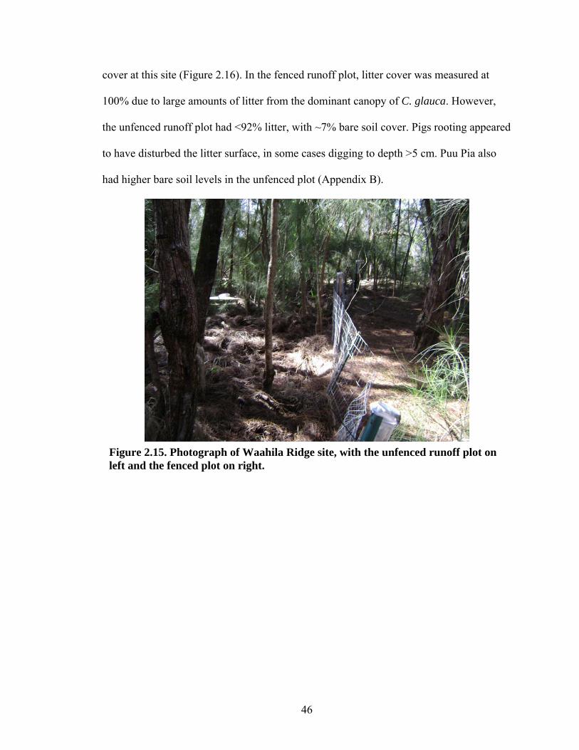
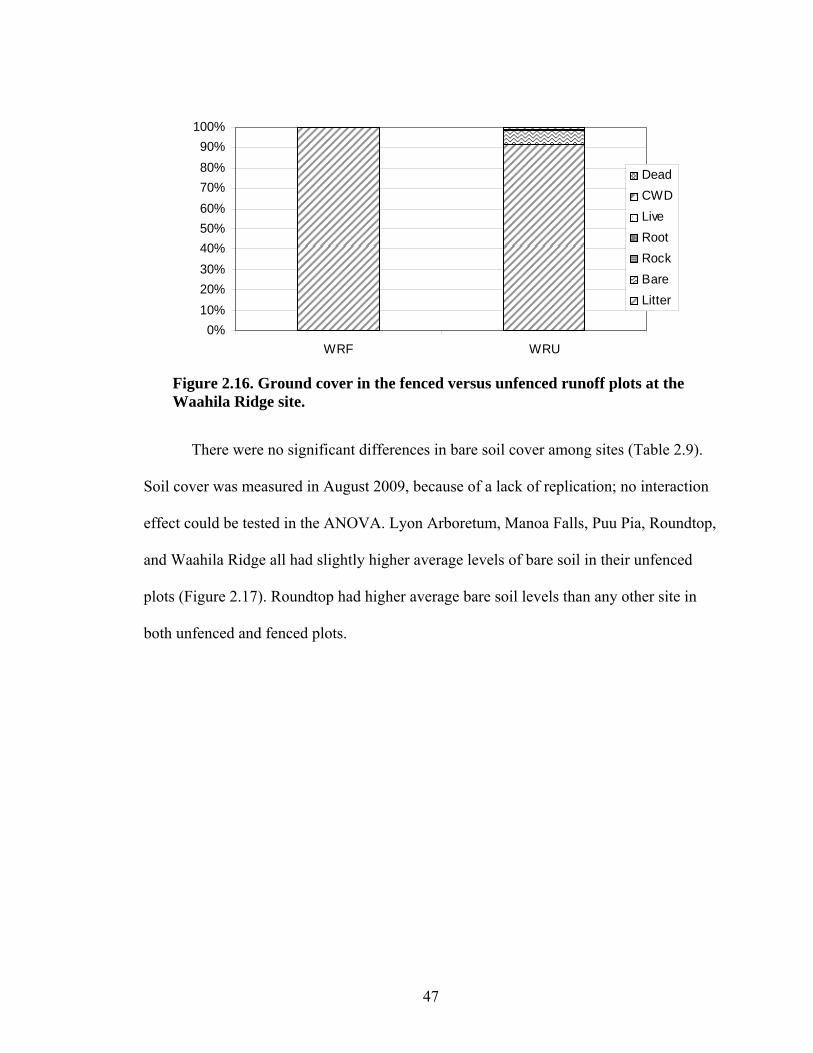
46
cover at this site (Figure 2.16). In the fenced runoff plot, litter cover was measured at
100% due to large amounts of litter from the dominant canopy of C. glauca. However,
the unfenced runoff plot had <92% litter, with ~7% bare soil cover. Pigs rooting appeared
to have disturbed the litter surface, in some cases digging to depth >5 cm. Puu Pia also
had higher bare soil levels in the unfenced plot (Appendix B).
Figure 2.15. Photograph of Waahila Ridge site, with the unfenced runoff plot on left and the fenced plot on right.
47
0%
10%
20%
30%
40%
50%
60%
70%
80%
90%
100%
WRF WRU
Dead
CWD
Live
Root
Rock
Bare
Litter
There were no significant differences in bare soil cover among sites (Table 2.9).
Soil cover was measured in August 2009, because of a lack of replication; no interaction
effect could be tested in the ANOVA. Lyon Arboretum, Manoa Falls, Puu Pia, Roundtop,
and Waahila Ridge all had slightly higher average levels of bare soil in their unfenced
plots (Figure 2.17). Roundtop had higher average bare soil levels than any other site in
both unfenced and fenced plots.
Figure 2.16. Ground cover in the fenced versus unfenced runoff plots at the Waahila Ridge site.
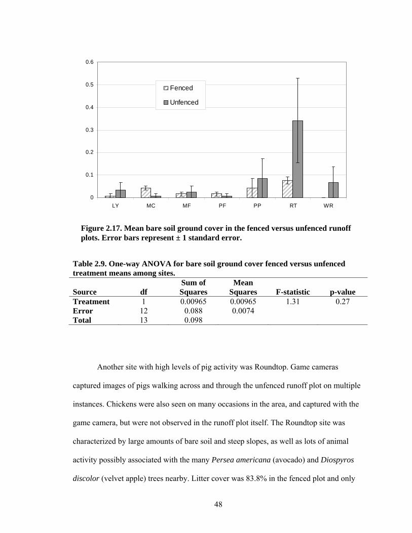
48
0
0.1
0.2
0.3
0.4
0.5
0.6
LY MC MF PF PP RT WR
Fenced
Unfenced
Table 2.9. One-way ANOVA for bare soil ground cover fenced versus unfenced treatment means among sites. Source
df
Sum of Squares
Mean Squares
F-statistic
p-value
Treatment 1 0.00965 0.00965 1.31 0.27 Error 12 0.088 0.0074 Total 13 0.098
Another site with high levels of pig activity was Roundtop. Game cameras
captured images of pigs walking across and through the unfenced runoff plot on multiple
instances. Chickens were also seen on many occasions in the area, and captured with the
game camera, but were not observed in the runoff plot itself. The Roundtop site was
characterized by large amounts of bare soil and steep slopes, as well as lots of animal
activity possibly associated with the many Persea americana (avocado) and Diospyros
discolor (velvet apple) trees nearby. Litter cover was 83.8% in the fenced plot and only
Figure 2.17. Mean bare soil ground cover in the fenced versus unfenced runoff plots. Error bars represent ± 1 standard error.

49
65.8% in the unfenced plot (Figure 2.18). Bare soil cover was 2.9% in the fenced plot and
8.2% in the unfenced plot. Live plant cover was higher in the fenced plot (11.0% vs.
9.0%), while coarse woody debris was higher in the unfenced plot (4.3% vs. 3.8%).
0%
10%
20%
30%
40%
50%
60%
70%
80%
90%
100%
RTF RTU
Dead
CWD
Live
Root
Rock
Bare
Litter
Finally, looking at the whole plot groundcover data (Figure 2.19), the percent
litter cover was slightly higher in the unfenced than the fenced plots, opposite to what
was seen in the runoff plots. However, levels of bare soil are similar (7.2% fenced and
7.0% unfenced), and the live plant, root, and rock cover all are higher in the fenced areas.
The only other ground cover higher in unfenced plots was standing dead vegetation.
Figure 2.18. Ground cover in fenced versus unfenced runoff plots at the Roundtop site.

50
0%
10%
20%
30%
40%
50%
60%
70%
80%
90%
100%
Fenced Unfenced
Dead
CWD
Live
Root
Rock
Bare
Litter
2.14 Runoff Volume
Across the study period runoff volumes ranged from <0.1 to >120 L. Runoff
volume on many occasions was greater than bucket capacity of 13.25 L, even with
collection feeder trays splitting off 50% of the runoff from Lyon Arboretum, Manoa
Cliffs, and Pauoa Flats. Overflow buckets results were analyzed separately because they
were installed only at Lyon Arboretum and Manoa Falls, even though many of the other
sites overflowed. Thus, runoff volumes in many cases are conservative estimates as
during the larger rain events almost every site exceeded runoff bucket capacity. For
example, during the large December event, every site except Waahila Ridge and the
Roundtop unfenced plot overflowed. In March, only the Waahila Ridge plots and the
Manoa Falls fenced plot did not overflow.
The repeated measures ANOVA indicated that month, site, site by month
interaction, and the site by treatment interaction all accounted for a significant proportion
Figure 2.19. Whole plot ground cover in fenced versus unfenced plots, average among all sites.

51
of the variance in the runoff volume data (Table 2.10). While runoff volume was
significantly different among months, there was also a significant site by month
interaction.
Table 2.10. Repeated measures ANOVA for runoff volume. Source
Num df
Den Df
Chi- Square
F-statistic
p-value
Month 10 60 948.40 94.84 <.0001 Site 6 60 1980.03 330.00 <.0001 Treatment 1 60 3.83 0.0503 0.055 Site x Month 60 60 1219.76 20.33 <.0001 Treatment x Month 10 60 8.31 0.83 .60 Site x Treatment 6 60 15.46 2.58 0.0275
The monthly pattern of runoff volumes followed a similar trend to throughfall
amounts, though there were some differences. December, as well as being the largest
throughfall event, was also the largest runoff event with 12.2 L (Figure 2.20). March was
the second-largest runoff event; averaging only 0.3 L less than December with 11.9 L.
July was the smallest throughfall event, and also by far the smallest average runoff event,
capturing less than half the volume of any other month. The month of October was an
exception to the trend, and had the second-lowest runoff volume (6.9 L, same amount as
June) despite being the fourth-largest throughfall event. The data also showed a seasonal
trend, with the wet season months of November, December, and March being
significantly larger runoff events than any dry season month except September. Besides
the September event, average runoff volume was higher in every wet season month than
any of the dry season months.

52
0
5
10
15
20
25
Vo
lum
e (
L)
Average runoff volume among sites showed a different pattern from the average
throughfall among sites. Lyon Arboretum received the most throughfall and also had the
highest average runoff volume (Figure 2.21). Manoa Cliffs, on the other hand, received
the fourth-highest throughfall but had the second-most runoff volume. Manoa Falls,
Pauoa Flats, and Puu Pia had statistically similar mean runoff amounts. The driest sites,
Roundtop and Waahila Ridge, showed no statistical difference in runoff amount.
Figure 2.20. Mean runoff volume in liters per rain event, among months. Error bars represent ± 1 standard error. Letters indicate significantly different means according to least squares means test.
A AB
ABC
CD
BCD
CD
A
DE CD
DE
E

53
0
5
10
15
20
25
30
LY MC MF PF PP RT WR
Vo
lum
e (
L)
The site by treatment interaction was a significant effect in the model. Manoa
Cliffs, Manoa Falls, Pauoa Flats, and Puu Pia had larger average runoff amounts from
unfenced plots (Figure 2.22). Conversely, Lyon Arboretum, Roundtop, and Waahila
Ridge had larger average runoff amounts from fenced plots. The largest average
difference between treatments was seen at Manoa Cliffs, with 15.4 L from the fenced
plot, and 18.46 L from the unfenced plot.
0
5
10
15
20
25
30
LYF MCF MFF PFF PPF RTF WRF
Ru
no
ff (
L)
Fenced
Unfenced
Figure 2.21. Mean runoff volume among sites in Liters per rain event. Error bars represent ± 1 standard error. Letters indicate significantly differences from least squared means.
Figure 2.22. Mean runoff volume in liters per rain event averaged across all plots. Error bars represent ± 1 standard error.
A
B
C C C
D D

54
During the December and March rain events, both plots at Lyon Arboretum
generated amounts of runoff in excess of the 128 L combined capacity of collection and
overflow buckets (Figure 2.23). This was a large volume of runoff from a 5.04 m2 area,
and was unexpected. However, this represents approximately 12-19 % of the total
throughfall volume from the December and March events at Lyon Arboretum. After
overflow bucket instillation, runoff at Manoa Falls exceeded the collection buckets only
during the December and March events. The largest total amount of runoff at Manoa
Falls was from the unfenced plot during the December event, with 43.3 L captured. This
represented 6-8 % of the total throughfall volume. Overall, the total runoff volume varied
from <1–16 % of total throughfall volume among the months. Lyon Arboretum had the
largest average runoff to throughfall ratio (7.8 %), while Waahila Ridge had the lowest
average runoff to throughfall ratio (2.9 %).
0
20
40
60
80
100
120
140
Dec Jan Feb Mar Apr
Ru
no
ff (
L)
LYF
LYU
MFF
MFU
Figure 2.23. Combined runoff volume from collection buckets and overflow buckets. Asterixs represent upper limit of volume (overflow of both buckets).
* * * *

55
2.15 Total Suspended Solids in Runoff
Across the study period, levels of TSS in runoff ranged from <0.01 to 7.05 g L-1
from individual plots. The repeated measures ANOVA indicated that TSS in runoff
differed significantly among months, but not among sites or between treatments (Table
2.11). There was also a significant site by month interaction. As indicated by the site by
month interaction, TSS levels were at times highly variable among sites, with CVs of
0.32-2.25.
Table 2.11. Repeated Measures ANOVA for TSS in runoff. Source
Num Df
Den df
Chi- Square
F-statistic
p-value
Month 10 60 599.14 59.91 <.0001 Site 6 1 194.76 32.46 0.13 Treatment 1 1 1.40 1.40 0.45 Site x Month 60 60 623.48 10.39 <.0001 Treatment x Month 10 60 9.87 0.99 0.46 Site x Treatment 6 1 8.65 1.44 0.56
December had the largest rain event with the most throughfall and also the highest
average TSS (Figure 2.24), more than double the amount of any other month. Though
February and April were small events overall the seasonal trend was still evident. The
wet season months of November, December, January, and March had higher mean TSS
in runoff than any of the dry season months. June, July, and August had the lowest mean
TSS in runoff, averaging >0.1 g L-1.
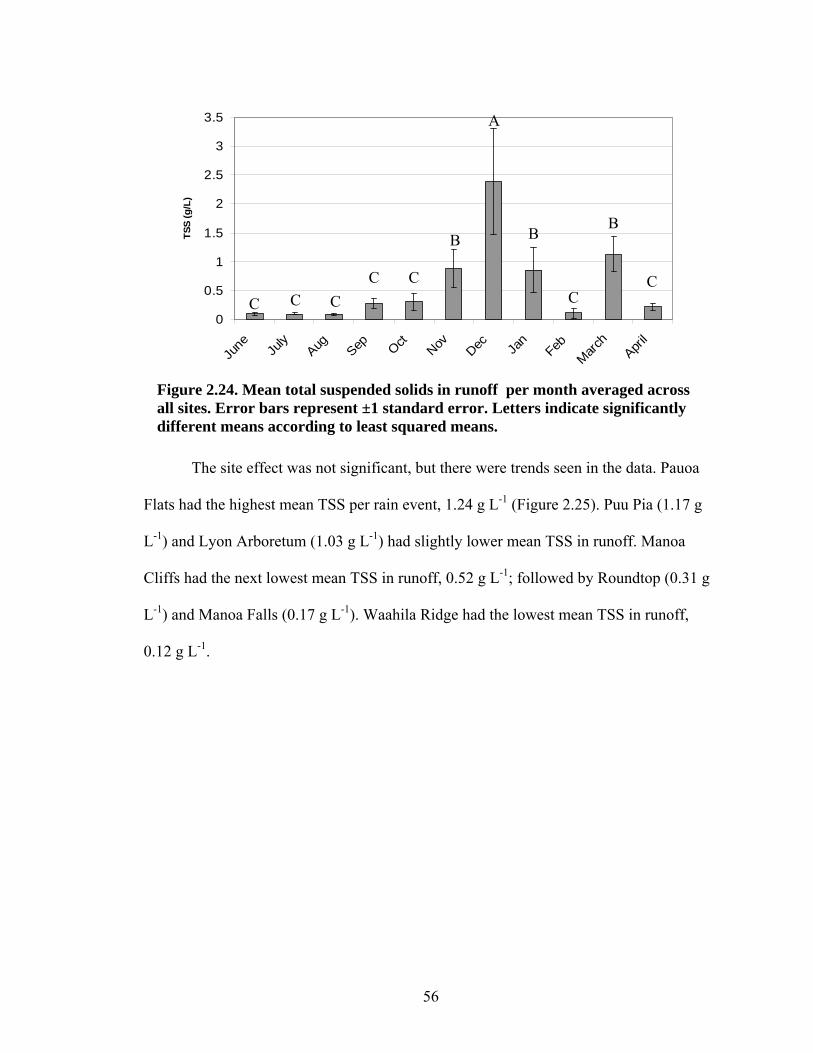
56
0
0.5
1
1.5
2
2.5
3
3.5
June Ju
ly Aug Sep O
ctNov
Dec Jan
Feb
Mar
chApr
il
TS
S (
g/L
)
The site effect was not significant, but there were trends seen in the data. Pauoa
Flats had the highest mean TSS per rain event, 1.24 g L-1 (Figure 2.25). Puu Pia (1.17 g
L-1) and Lyon Arboretum (1.03 g L-1) had slightly lower mean TSS in runoff. Manoa
Cliffs had the next lowest mean TSS in runoff, 0.52 g L-1; followed by Roundtop (0.31 g
L-1) and Manoa Falls (0.17 g L-1). Waahila Ridge had the lowest mean TSS in runoff,
0.12 g L-1.
Figure 2.24. Mean total suspended solids in runoff per month averaged across all sites. Error bars represent ±1 standard error. Letters indicate significantly different means according to least squared means.
A
B B
C
B
C C
C C
C
C

57
0.0
0.2
0.4
0.6
0.8
1.0
1.2
1.4
1.6
1.8
LY MC MF PF PP RT WRSite
TS
S (
g/L
)
The month by treatment interaction was not significant, but there did appear to be
a slight trend in the data. Seven of the eleven months had higher mean TSS in runoff
from unfenced plots, while only three months had higher mean TSS from the fenced plots
(Figure 2.26). In April, mean TSS in runoff was equal between fenced and unfenced
plots.
Figure 2.25. Mean total suspended solids in runoff per site averaged across all months. Error bars represent ± standard error. Letters indicate significantly different means according to least squared means.
A
A
B
A A
A
B
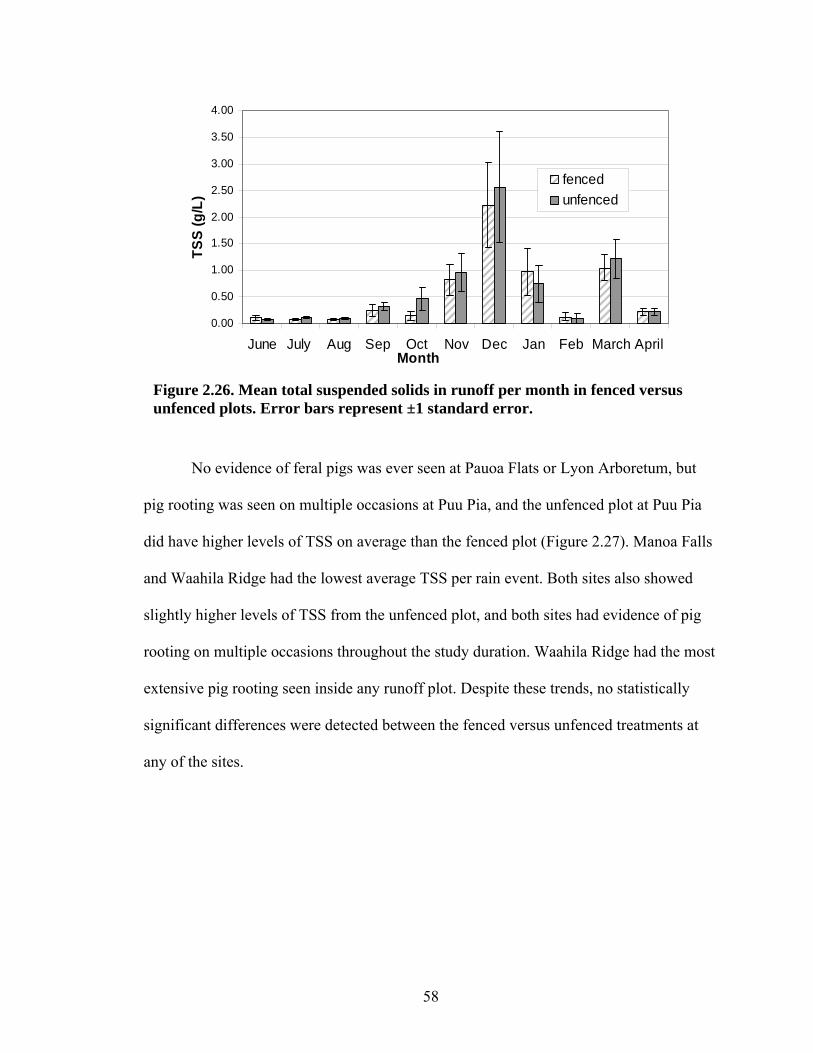
58
0.00
0.50
1.00
1.50
2.00
2.50
3.00
3.50
4.00
June July Aug Sep Oct Nov Dec Jan Feb March AprilMonth
TS
S (
g/L
)fenced
unfenced
No evidence of feral pigs was ever seen at Pauoa Flats or Lyon Arboretum, but
pig rooting was seen on multiple occasions at Puu Pia, and the unfenced plot at Puu Pia
did have higher levels of TSS on average than the fenced plot (Figure 2.27). Manoa Falls
and Waahila Ridge had the lowest average TSS per rain event. Both sites also showed
slightly higher levels of TSS from the unfenced plot, and both sites had evidence of pig
rooting on multiple occasions throughout the study duration. Waahila Ridge had the most
extensive pig rooting seen inside any runoff plot. Despite these trends, no statistically
significant differences were detected between the fenced versus unfenced treatments at
any of the sites.
Figure 2.26. Mean total suspended solids in runoff per month in fenced versus unfenced plots. Error bars represent ±1 standard error.

59
0.0
0.5
1.0
1.5
2.0
2.5
LY MC MF PF PP RT WRSite
TS
S (
g/L
)
Fenced
Unfenced
2.16 Correlation of TSS with Environmental Variables
Many variables are thought to be associated with runoff generation and erosion.
In order to understand their relationships and influence on TSS, a Spearman correlation
was conducted. A correlation matrix (Table 2.12) showed TSS to be positively correlated
with throughfall, soil moisture, and coarse woody debris cover. Coarse woody debris had
the highest correlation with TSS (r = 0.73, p = 0.003). The other ground cover variables
(bare, litter, live, rock, root) did not significantly correlate with TSS. Neither basal area
nor stem density were significantly correlated with TSS, but they were positively
correlated with each other (r = 0.61, p = 0.02). Ksat values did not correlate with any
other variable, though basal area and Ksat were correlated (r = 0.51, p = 0.06).
Overall, the most influential variable in the correlation analysis was throughfall,
as it was correlated to five other variables. In addition to TSS, throughfall was also
correlated with soil moisture, rock cover, live cover, and runoff amount. The relationship
Figure 2.27. Mean total suspended solids (TSS) per plot. Error bars represent ±1 standard error.

60
among throughfall, soil moisture, and runoff amount seems straightforward, given
general knowledge of the hydrologic cycle. The relationship of throughfall with the other
two ground cover variables is less obvious. Live plant cover had the highest correlation
with throughfall (p = 0.0003) of all environmental variables. Slope and soil moisture
were also important variables in the correlation. Both of these variables were
significantly correlated with four of the other environmental variables. Slope was
negatively correlated with soil moisture, and positively correlated with bare soil cover,
stem density, and basal area. It is interesting that slope was correlated positively with
both the forest structure variables, suggesting more and larger trees at the sites with
steeper slopes. Soil moisture was negatively correlated with basal area, and positively
correlated with slope. Slope was positively correlated with TSS and throughfall. Among
the ground cover variables, only litter did not correlate with any other factor. Rock cover
was positively correlated with throughfall and runoff amount.
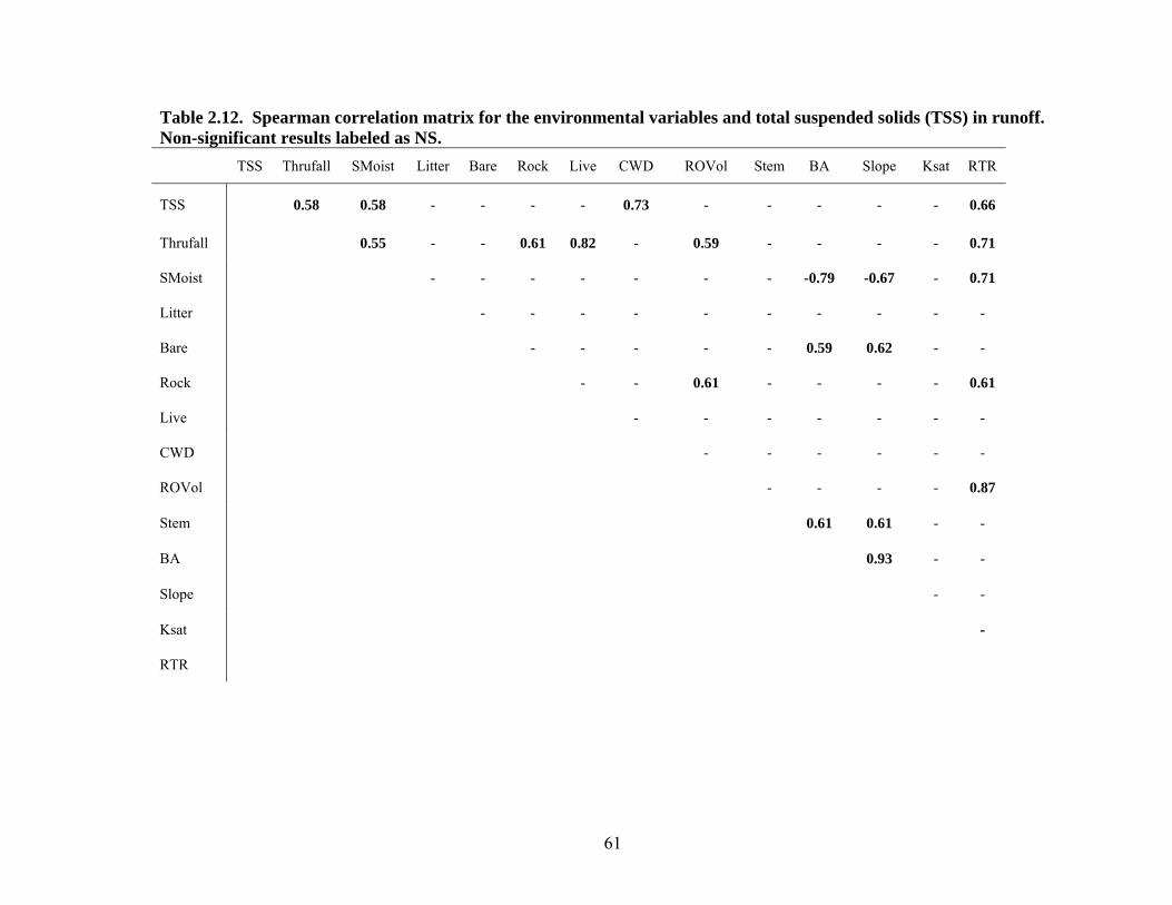
61
Table 2.12. Spearman correlation matrix for the environmental variables and total suspended solids (TSS) in runoff. Non-significant results labeled as NS.
TSS Thrufall SMoist Litter Bare Rock Live CWD ROVol Stem BA Slope Ksat RTR
TSS 0.58 0.58 - - - - 0.73 - - - - - 0.66
Thrufall 0.55 - - 0.61 0.82 - 0.59 - - - - 0.71
SMoist - - - - - - - -0.79 -0.67 - 0.71
Litter - - - - - - - - - -
Bare - - - - - 0.59 0.62 - -
Rock - - 0.61 - - - - 0.61
Live - - - - - - -
CWD - - - - - -
ROVol - - - - 0.87
Stem 0.61 0.61 - -
BA 0.93 - -
Slope - -
Ksat -
RTR

62
Throughfall, soil moisture, and coarse woody debris were input into a multiple-
stepwise regression. The analysis indicated all three were significant predictors of TSS
(Equation 1).
Equation 1. Model for predicting TSS, based on multiple-stepwise regression (r = 0.58, p = 0.05).
2.17 Discussion
The first objective of this chapter was to quantify throughfall, runoff volume, and
TSS in runoff from forested areas of the Manoa watershed. Runoff and throughfall were
recorded from one rainfall event per month for each of the 7 sites, from June 2008
through April 2009. Runoff volumes overwhelmed the collection capacity at many of the
sites, but the installation of overflow buckets helped better quantify the extremely large
volumes of runoff generated during wet season rain events in the upper watershed. As
predicted, runoff volumes were significantly higher in many of the wet season months
than the dry season months. November, December and March were the largest runoff
events, all in the wet season, and significantly larger than any dry season month except
September. Though September was a larger runoff event than February and April, it was
the only dry season month that had larger runoff volumes than any of the wet season
months.
The Repeated Measures ANOVA showed a significant difference between
treatments at α = 0.1, but this was confounded by a significant site by treatment
interaction. Runoff volumes were also different among sites but this was confounded by a
significant site by month interaction. In general, Lyon Arboretum had more runoff than
TSS = -0.63 + 0.1(Throughfall) + 1.68(SoilMoisture) + 10.50(CoarseWoodyDebris)

63
any other site, as well as more throughfall. Pauoa Flats, Puu Pia, and Manoa Falls all had
similar amounts of runoff, despite being quite different in terms of forest structure, slopes
and soils. Pauoa Flats was an interesting site because during many of the dry season
months (June, July, September, and October) no runoff was produced; however during
the larger wet season events (December and March) runoff exceeded collection bucket
capacity. Lau and Mink (2006) show initiation times for runoff varies considerably in
Hawaiian soils, from just a few minutes to more than 60-80 minutes, depending on
antecedent saturation deficit and soil type. Another important result was the sheer amount
of runoff generated from these small plots. Despite the fact that runoff plots drained an
area of only 5.04 m2, the amounts of runoff were extremely large, ranging from 7.5 to
26.5 L in December, especially when factoring in the overflow bucket data from Lyon
Arboretum (at least 128 L total runoff). In a study of agricultural runoff plots in Hawaii,
Ryder and Fares (2008) found runoff volume varied from 0.37 – 12.23 L, though it
appears runoff may have exceeded bucket capacity during the largest event in their study.
Throughfall quantification was aided by the installation of four extra gauges at
each site. The additional gauges gave a more extensive view of throughfall levels and the
within site variability of throughfall at these sites. The average throughfall per site
matched rainfall distributions (Figure 2.28), the only discrepancy being that the Manoa
Falls site had higher average throughfall than the Manoa Cliffs site even though Manoa
Cliffs was in a higher rainfall area. The Manoa Cliffs canopy, with Hibiscus arnottianus,
C. nocturnum, and C. burmanni had a much different composition than Manoa Falls,
which was heavily dominated (>95% stems) by P. cattleianum. Only one rain event per
month was captured, and yet monthly rainfall data (Figure 2.29) from the USGS Real-

64
Time Manoa Rain Gauge (USGS 211747157485601 711.6, Kanewai Fld, Honolulu,
Oahu, HI), showed a similar pattern to throughfall. December had the largest amount of
rainfall at Manoa Rain Gauge (MRG) and the highest average throughfall at the study
sites, followed by March and November with the next highest rainfall levels at MRG and
the next highest average throughfall. The rainfall data also showed the ‘wet season’
months of January and February having less rainfall then the ‘dry season’ month of
October.
Quantification of TSS in runoff showed significant differences among months and
a significant site by month interaction. Though the estimates of runoff amount were
conservative (i.e. underestimated during certain high rainfall events), TSS was measured
on a g L-1 basis and therefore did not depend on the quantification of full runoff amount.
These results showed TSS levels that for certain events appeared quite large for heavily
forested areas. For example, the Puu Pia unfenced runoff plot yielded 7.05 g L-1 during
the December event, which was comparable to agricultural studies that measured TSS in
runoff from cultivated fields at >10 g L-1 (Borina et al., 2005). Ryder and Fares (2008)
found TSS levels ranged from 41.3 g L-1 in a fallow plot after an extremely large rain
event, to 0.04 g L-1 after a small rain event in a plot with vegetative cover of oats. A
hydrological study of TSS in streams and channels in Georgia (Shelby et al., 2006) found
levels ranged from 0.02 – 0.35 g L-1. De Carlo et al. (2007) found TSS levels at the outlet
of three streams into Kaneohe Bay, Oahu (0.0008 - 0.019 g L-1) were often several orders
of magnitude less than levels found from the runoff plots in this study.

65
0
50
100
150
200
250
Jun Jul Aug Sep Oct Nov Dec Jan Feb Mar Apr
Rai
nfa
ll (
mm
)
Figure 2.29. Rainfall per month from USGS Kanewai Field rain gauge. Asterix denote provisional data subject to revision.
Figure 2.27. Isohyetal rainfall pattern and location of sites in Manoa Watershed.
*
*
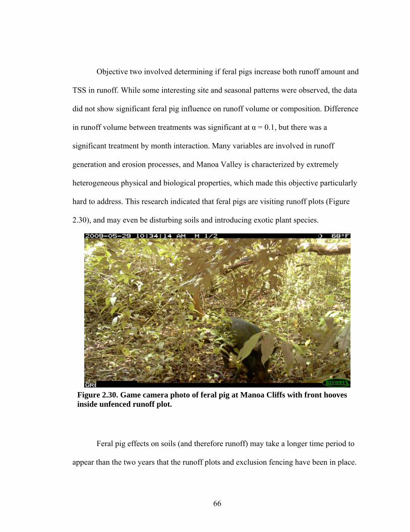
66
Objective two involved determining if feral pigs increase both runoff amount and
TSS in runoff. While some interesting site and seasonal patterns were observed, the data
did not show significant feral pig influence on runoff volume or composition. Difference
in runoff volume between treatments was significant at α = 0.1, but there was a
significant treatment by month interaction. Many variables are involved in runoff
generation and erosion processes, and Manoa Valley is characterized by extremely
heterogeneous physical and biological properties, which made this objective particularly
hard to address. This research indicated that feral pigs are visiting runoff plots (Figure
2.30), and may even be disturbing soils and introducing exotic plant species.
Feral pig effects on soils (and therefore runoff) may take a longer time period to
appear than the two years that the runoff plots and exclusion fencing have been in place.
Figure 2.30. Game camera photo of feral pig at Manoa Cliffs with front hooves inside unfenced runoff plot.

67
The effect of feral chickens (Gallus gallus domesticus), mongooses (Herpestes
javanicus), and rats (Rattus sp.), particularly at the Roundtop site, was another variable
that was not quantified and which had the ability unlike the feral pigs, to bypass
exclusion fencing by climbing through or over, or flying above fences to disturb litter and
soils and potentially increase erosion.
The third objective was to investigate temporal and spatial differences in TSS
levels in runoff. Results show TSS levels exhibited strong seasonal trends, with
significantly higher values in many of the wet season months than the dry season months.
For example, November, December, January, and March all had significantly larger TSS
amounts than any of the dry season months. Total SS appeared to be highly influenced by
the magnitude of throughfall of an individual rain event, and TSS and throughfall were
significantly correlated. The December rain event had significantly higher throughfall
than any other month, and significantly higher levels of TSS. Spatial variation of TSS
levels was high, with Puu Pia and Pauoa Flats >1.1 g L-1; while Manoa Falls and Waahila
Ridge were both <0.2 g L-1. Puu Pia and Pauoa Flats were physically different sites, yet
had similar average levels of TSS in runoff. Puu Pia had the highest stem density and
basal area of any site, while Pauoa Flats had the lowest stem and the second smallest
basal area. Puu Pia also had the steepest slope, while Pauoa Flats, as the name suggests,
had the lowest slope. No pig disturbance was ever seen at Pauoa Flats, while evidence of
pig rooting was seen on multiple occasions at Puu Pia. The pig activity at Puu Pia could
be an explanation of why TSS in runoff was so high despite the high stem density and
lower levels of throughfall.

68
The final objective of this study was to investigate correlations between
environmental variables and TSS in runoff. Total SS was significantly correlated with
throughfall, soil moisture, and coarse woody debris cover. The correlation with
throughfall could indicate that more throughfall means more opportunity for physical
detachment of soil particles. Also, because overland flow is blocked from entering the
runoff plots, the process of soil erosion from the plots was assumed to be caused by
detachment of soil particles from the physical impact of falling droplets inside the plot.
Since the rainfall events were typically only one or two day episodes, it would
seem likely that the larger rainfall events involved higher rainfall intensity. In field
experiments, Grace (2008) found total precipitation, average rainfall intensity, and
maximum 30-minute rainfall intensity were detected as the most influential storm
characteristics in determining soil erosion. It was surprising that coarse woody debris had
the strongest correlation with TSS, and it was not obvious why such a relationship would
exist. It could be that the coarse woody debris (defined as tree litter with >2.0 cm
diameter) are related to the larger tree species (e.g. E. grandis) with taller canopies that
cause throughfall to have greater velocity when striking the soil surface, causing soil
particle detachment. Though I hypothesized that ground cover in general would correlate
with TSS in runoff, it seemed more likely that bare soil or litter would have a stronger
relationship with TSS than coarse woody debris. However, neither bare soil nor litter had
significant correlations with TSS. This may have to do with the highest levels of bare soil
being at Roundtop, which was one of the driest sites and averaged low levels of TSS.
Bare soil levels were overall quite low, considering the high amounts of sediment coming
off the plots at times. Besides Roundtop, litter cover levels were overall quite high, above

69
60% even at Roundtop, and as high as 100% at Waahila Ridge. Litter protects the soil
surface from raindrop impact and slows overland flow, reducing erosion.
Soil moisture is a significant factor in determining runoff generation (Lau and
Mink, 2006). Browning’s (2008) study at the same sites found that TSS in runoff was
also correlated with soil moisture. He found that TSS was also correlated with runoff
amount, canopy cover, and bare soil cover. However, his estimation of bare soil cover
involved a different (and coarser visual estimation) method than the line-transect method
I employed. There also could have been an even higher correlation between TSS and soil
moisture except for the fact that soil samples were taken in the first dry period of each
month during the activation process. Because rain events are hard to predict and
activation was initiated regardless of the long-term weather pattern, there was often a lag
time between site activation/soil sampling and rainfall events. This lag time ranged from
three days to almost two weeks. This meant that soil moisture levels could be quite
different from what was originally measured once the rain event arrived.
Most Hawaiian soils are known to absorb water readily (Lau and Mink, 2006)
with infiltration rates ranging from 0.043-0.51 m hr-1 depending on soil type (USDA,
1972). Reduction in infiltration as a result of various land uses (crop production,
urbanization) was also reported. Ksat values between 0.3 and 1.2 m day-1 (0.0125 and
0.05 m hr-1) were reported from forested sites near Lyon Arboretum (Lau and Mink,
2006). Antecedent soil conditions, however, were seen to affect infiltration, with an
approximately 50% reduction during wet conditions. The data showed large differences
among sites, and even among plots at the same site. For example, Ksat at the Lyon
Arboretum site in this study was calculated to be 0.055 m hr-1 in the unfenced plot, but

70
the fenced plot was calculated at 21.75 m hr-1, or almost 500 times larger. Some of the
calculated values from other sites are in that 0.013-0.05 m hr-1 range, but many are orders
of magnitude larger, and some even smaller. There could be several reasons why data
was so variable. First, was the fact that this instrument was designed to be used on level
ground, and the sites in this study had slopes ranging from 6-26%. Second, there was also
the problem of finding a homogenous soil surface inside the site without roots, rocks, or
other debris, and without being inside the runoff plot itself.
Though the basal area and stem density were not correlated to TSS, they did help
illustrate the heterogeneity of the watershed and the physical and biological differences
between sites. The seedling and sapling data may help illuminate the effects of feral pigs
in the upper watershed areas. Psidium cattleianum was of particular interest because it is
a well-documented food source of feral pigs (Huenneke et al., 1990; Noguiera et al.,
2007), and its seeds are spread in pig feces (Diong, 1982). Pigs also increase soil fertility,
which may impede the reestablishment of native plant species adapted to nutrient-poor
environments (Noguiera-Filho et al., 2009). The sapling and seedling counts showed
close to twice as many individuals in the unfenced versus the fenced plots. This could be
an effect of pig presence, and though this data was not a main focus of the study, it is
nonetheless an interesting result. A study in Big Thicket National Preserve, Texas, found
exotic Sapium sebiferum (Chinese tallow tree) was twice as abundant in plots with feral
pigs present (Siemann et al., 2009). Cinnamomum burmanni seedlings are not thought to
be spread by feral pigs, but the many seedlings found are indicative of the highly invasive
nature of this tree in Hawaii (Starr et al., 2003). It is actively invading many mesic forests
and is known for dense monotypic stands and extremely high seedling recruitment, even

71
in low light conditions. Pig disturbance could help create favorable conditions for
seedling recruitment. The tree produces small fruits that are thought to be dispersed by
birds.
2.18 Conclusions
Hypothesis one predicted that TSS would be higher in the wet season than the dry
season, and the results of this study generally supported this hypothesis. The repeated
measures ANOVA showed significantly different levels of TSS among months although
there was also a significant site by month interaction, indicating that the trends were not
always consistent across all sites. This suggests that resource managers should be more
concerned about runoff and sedimentation from the upper forested areas of Hawaiian
watersheds during the months of November-April. Sediment traps, such as those used at
construction sites, coir logs, or vegetative strips could be applied to areas with high
overland flow to help decrease the amount of sediments reaching streams and waterways.
Certain activities, such as construction and trail maintenance could be curtailed during
the wet season. The wet season may also be a time when feral pigs are more active, and
move lower in the watershed (Hone, 2002). Pig population control methods could be
encouraged during the wet season, and perhaps hunting limitations relaxed.
Hypothesis two predicted that TSS would be higher in unfenced plots than fenced
plots. My data did not support this hypothesis. The repeated measures ANOVA showed
no significant difference between plots. Many factors influence runoff generation and
erosion, and the heterogeneity of the landscape in the upper forested areas of Manoa
watershed made it hard to determine what, if any, effects feral pigs were having on

72
runoff. Also, the plots had only been in place for one year prior to the start of this study,
and differences may yet manifest. Some of the sites (Puu Pia, Roundtop) had much
higher levels of TSS in the unfenced plots, and these sites did see multiple occurrences of
pig rooting.
Hypothesis three predicted that ground cover and soil moisture would have the
highest correlation with TSS in runoff. This hypothesis was partially supported by the
data. Soil moisture and coarse woody debris, along with throughfall amount, were
significantly correlated with TSS. A correlation with soil moisture was also found in an
earlier study at these sites by Browning (2008). Soil particles in wetter soils may be more
susceptible to dislodgement by water droplet impact or overland flow. There could also
be a relationship among sites with moister soils and higher levels of TSS in runoff. Soil
moisture was determined by laboratory methods, but handheld devices exist that allow
for instantaneous determination of soil moisture in the field. Such devices may assist
resource managers in identifying areas of concern for high TSS generation.
Coarse woody debris was not the ground cover variable expected to correlate best
with TSS. Litter cover and bare soil cover were expected to be more important in
determining TSS in runoff. Coarse woody debris may be associated with another factor
that is important to runoff generation and TSS in runoff. Coarse woody debris were
defined as litter >2.0 cm diameter, which are therefore associated with larger trees. Many
of the P. cattleainum, C. nocturnum, and other species of tree measured DBH only
slightly larger than 2.0 cm in diameter. Most litter from these trees would be expected to
have diameter <2.0 cm. Perhaps TSS in runoff is associated with trees such as E. grandis
and E. robusta that were on average much larger in diameter. Such a relationship could

73
help guide resource managers charged with protecting water quality in targeting efforts of
exotic tree removal or containment. Coarse woody debris may also represent canopy gaps
where raindrops fall unhindered, striking the soil surface with greater force and more
often detaching soil particles.
Comparative studies of fencing to exclude feral pigs or inhibit their access into
sensitive forested areas are few (Campbell and Long, 2009), and these runoff plots
provide an excellent opportunity to study feral pig impacts on water quality, soils, and
vegetation. Using paired runoff plots in a forested setting is a novel approach; the
literature review found no other similar studies besides Browning’s (2008) research at
these same plots. Besides elucidating site and seasonal differences in runoff, this study
provides baseline conditions for further research at the runoff plots. As time goes on, I
expect differences between fenced and unfenced plots will continue to develop, and
further research is needed at these sites to document these dynamics.

74
CHAPTER 3: ENTEROCOCCI IN RUNOFF AND SOILS 3.1 Introduction
This study aims to improve our understanding of the processes of runoff and soil
erosion in upper forested areas of a Hawaiian watershed and to identify the effects pigs
have on erosion, runoff, water quality, and fecal indicator bacteria (Enterococcus sp.). It
is thought that feral pigs can not only harm native flora and fauna but may even adversely
impact the health and function of entire watersheds (Noguiera-Filho et al., 2009). Such
effects also raise important concerns for public health. From Santa Monica Bay, CA to
the Great Lakes, levels of indicator bacteria have been shown to correlate with incidence
of illness reported by swimmers (Haile et al., 1999; Wade, 2006). Though some research
suggests that Enterococci are free-living and reproduce in Hawaiian soils (Hardina and
Fujioka, 1991), mesocosm experiments have found that Enterococci do not multiply in
subtropical waters and sediments (Anderson et al., 2005). This study will aid natural
resource managers and policy makers, helping them identify the effects of feral pigs, if
any, and informing them of the effectiveness of fencing as a tool for improving water
quality.
The specific objectives of this chapter are as follows: (1) Quantify Enterococci in
runoff and soils from forested areas of Manoa watershed; (2) Determine if feral pigs
impact Enterococci in runoff and soils; (3) Investigate temporal and spatial differences in
Enterococci levels in runoff; and (4) Investigate correlations among environmental
variables (slope, infiltration rate, soil moisture, stem density, etc) and Enterococci in
runoff. Given what was learned in the literature review, and drawing on the results of

75
previous research at these sites (Browning, 2008), I developed four hypotheses: (1)
Higher storm intensity and higher throughfall inputs will lead to higher Enterococci
levels in runoff during the wet season (November-April) than in the dry season (May-
October); (2) Fecal contamination will lead to higher Enterococci levels in runoff and soil
at unfenced plots exposed to feral pig activity; (3) Of all environmental predictors
measured, ground cover and soil moisture will have strongest correlations with
Enterococci in runoff as ground cover influences soil erosion processes, and Enterococci
survival is thought to be higher, and infiltration is lower under wetter soil conditions
which directly affect runoff production; (4) TSS in runoff will positively correlate with
Enterococci abundance in runoff as bacteria are thought to associate with soil particles in
surface waters.
Materials and Methods
3.2 Site Selection
In the spring of 2007, eight sites were selected to investigate runoff processes and
the effects of feral pig exclusion in the Manoa watershed. The sites were chosen from the
upper forested areas of the watershed, based on attributes of slope, accessibility, and
vegetation. Slope was the primary determining factor in initial site selection to allow for
construction of exclusion fencing and to ensure collection of accurate runoff data.
According to Mutchler et al. (1994) a slope of 9% or less is considered the standard in
most agricultural studies that incorporate runoff plots; however areas with <9% slope
were not easy to find as the average slope of the watershed is 47%. Using a Geographic

76
Information System (GIS), a map of slope characteristics throughout the watershed was
created and areas with slopes between 5-30% were identified as potential sites (Fig. 3.1).
Final site selection was based on ease of accessibility and proximity to existing trail
networks as well as homogeneity of slope/vegetation at each site (Table 3.1).
Unfortunately the Palolo site was vandalized repeatedly throughout the study period and
had to be abandoned, leaving only seven sites for this study.
Figure 3.1. A GIS map of the variation in slope across the Manoa watershed with the locations of original eight sites of study.

77
Table 3.1. Characteristics of the seven sites in Manoa watershed. Elevation and soil series information were obtained through a GIS analysis, while slopes were recorded on site using a handheld clinometer. Site Elevation (m) Slope (%) Soil Series
Lyon 215 15.5 Lolekaa
Mānoa Cliffs 450 8 Rough Mountainous Land
Mānoa Falls 171 17 Lolekaa
Pauoa Flats 538 6 Rough Mountainous Land
Puu Pia 209 26 Lolekaa
Round Top 340 25.5 Tantalus
Waahila Ridge 340 14 Manana
3.3 Site Layout
Each site is approximately 10 meters long by 10 meters wide. Two paired 10 m by
5 m runoff plots were established at each site; one runoff plot surrounded by exclusion
fencing, the other unexclosed. Runoff plots were oriented down the slope to effectively
capture the natural path of overland flow at each site. Fences were constructed of 14-
gauge utility fencing 0.91 m tall and held in place with metal posts. Barbed wire was
strung along the bottom edge of each fence to provide further protection from pig
damage. During construction, throughfall gauges were affixed to posts directly centered
between the paired plots at each site. In December 2008, four more throughfall gauges
were added to each site (Figure 3.2).

78
Figure 3.2. The basic layout of each of the seven sites. Each site was oriented so both fenced and unfenced plots had similar slope and vegetation.
3.4 Runoff Plot Design
Following fence installation, runoff plots were constructed within both unfenced
and fenced plots at each site. Runoff plots are approximately 4.2 m long by 1.2 m wide,
oriented down the prevailing slope of each site. To prevent additional runoff entering
from outside the plot, 15 cm tall plastic dividers were buried roughly 7.5 cm into the soil
along the upslope and outer edges of each runoff plot. These plastic pieces formed the
framework that channeled runoff to a central collector (Fig. 3.2). This central collector
was located at the down slope end of the runoff plot, consisting of a triangular metal
runoff collector that funneled all runoff into a 10 by 5 cm opening (Fig. 3.2). A metal
feed tray connected the metal collector to an 18.9 L bucket for storing runoff. A

79
rectangular hole was cut into the side of the bucket into which the feed tray drained.
Water-tight lids were affixed to the top of each bucket to prevent throughfall from
directly falling into the bucket. Sheet metal collector covers were constructed to also
prevent direct throughfall on the metal collector and installed in December 2008.
3.5 Activation Periods and Runoff Sampling
Runoff samples were collected from June 2008 to April 2009 to ensure collection
of samples from both the wet and dry seasons. At the beginning of each month a two-day
dry period was targeted to activate all plots and initiate runoff collection. Activation of
each site included emptying all throughfall gauges, collecting soil samples for moisture
analysis, and emptying/cleaning the runoff collection buckets. Runoff was removed with
a hand operated suction pump, and then paper towels were used to clean and dry all
inside surfaces of collection buckets. Sterile latex gloves were worn at all times during
emptying and cleaning procedures. Collection times were determined by observing
weather conditions and monitoring the online USGS rain gauge located in Mānoa Valley.
When the rain gauge recorded a significant rainfall (typically > 2 cm) during the active
period, collection was initiated.
The collection process involved measurement of total runoff and collection of
runoff sub-samples to be analyzed for TSS. During all activation and collection
activities, care was taken to avoid walking within runoff plots. Soil samples were taken
within the sites, yet outside the runoff plots so as not to disturb soils. In the duration
between observation periods runoff was allowed to continue its natural flow into the
buckets. If the buckets began to overflow, runoff simply drained out through the same

80
opening from which it entered and continued flowing down slope. Throughfall gauges
were covered with duct tape while not active.
3.6 Estimation of Other Environmental Variables
As this project was designed to monitor runoff and sediment loss from the study
areas and to develop correlation and regression equations for TSS in runoff, it was
important to quantify a variety of different variables that influence these processes. This
required recording of site characteristics throughout the duration of the study, as well as
prior to rain events, and also the analysis of runoff after the events. The other
environmental variables recorded were slope, soil series, soil water content, throughfall,
infiltration rate, forest canopy and understory species composition, stem density, basal
area of trees, seedling/sapling counts, and ground cover assessment. The following
paragraphs summarize the methodology used to determine these characteristics.
3.6.1 Slope Recordings
Slopes were measured using a handheld clinometer and ranged from 5% to 27%.
No site was recorded to have greater than a 2% difference between the fenced and
unfenced plots. Ultimately, all seven sites represented a range of different slope types as
shown in Table 3.1.
3.6.2 Soil Series Determination
Soil series for each site were retrieved from NRCS soil maps. Additionally,
global positioning system (GPS) coordinates for each site recorded in the field were

81
added to the GIS. These two data layers were overlaid to identify the soil series of each
site based on the latest soil survey of Oahu (Foote et al. 1965). The seven sites
represented four different soil series; Tantalus, Lolekaa, Manana, and Rough
Mountainous Land (rRT) (Table 3.1).
3.6.3 Calculation of Soil Water Content
Gravimetric soil water content, was determined during the activation phase of
each month. A 2 cm diameter soil corer was used to collect samples from approximately
the upper 5 cm of the soil profile. One composite sample was collected during site
activation from both the fenced and unfenced areas. The composite sample consisted of
three separate randomly-located individual samples from each area, combined in a sterile
plastic bag. No soil samples were taken from within runoff plots to avoid disturbing
soils. Percent gravimetric soil moisture was calculated by the equation:
% Gravimetric Soil Moisture = ( 1 - (dry mass soil / wet mass soil) ) x 100
3.6.3. Infiltration Rates
Infiltration rate and the coefficient of saturation (Ksat) were determined at each
plot using a Tension Infiltrometer (8 cm model, Soil Measurement Systems, Tucson,
AZ). The most level and uniform area of each fenced/unfenced plot (although not within
the runoff plot areas) was chosen as the infiltration measurement site. A metal spatula
was used to cut out a shallow hole in the litter layer the same size/shape as the
infiltrometer base to expose the soil surface. A layer of fine sand was added to the hole.
The infiltrometer was then filled with water and placed on the sand layer. The tension

82
was set to 11 cm. If infiltration did not commence, tension was lowered to 10 cm.
Readings of water level were taken every 30 seconds for 10 minutes, then every 60
seconds for another 10 minutes, and a final reading was taken after five more minutes.
The tension was then lowered to 8 cm if initial tension was 11 cm, 7.5 cm if initial
tension was 10 cm. This was to ensure enough of a tension difference between the two
readings to allow for calculation of Ksat.
Equilibrium infiltration slopes were determined graphically. The slope was then
multiplied by the area of the infiltrometer’s base to determine the volume of water
infiltrated per time. Ksat was calculated from the equation:
α = LN (Infiltration rate X / Infiltration rate Y) (- Tension X - Tension Y)
Ksat = Infiltration rate X Area of base ^ (α * Tension X) * (1 + 4 / Area of base * α)
Where X = tension 1, and Y = tension 2
3.6.4 Throughfall Recording
A standard all-weather rain gauge (Productive Alternatives, Fergus Falls, MN)
was used to measure throughfall (mm) of rain events. As part of the activation process,
each throughfall gauge was emptied and a thin layer of mineral oil was added to prevent
evaporation
3.6.5 Forest Structure Characterization
The seven sites in Manoa Valley varied in terms of forest structure and species
composition. To quantify these differences, a 20 m by 20 m plot directly surrounding

83
each site was established and all trees > 2 cm diameter at breast height (DBH) were
measured. DBH is defined as diameter at 1.32 m from the ground surface. Species was
recorded for each tree in the plot. If a tree could not be identified to the species level in
the field, a leaf sample was taken back to the lab for identification. Stem density (# stems
ha-1) was calculated by counting the number of stems in the 400 m2 plot and scaling to a
hectare basis. Basal area (cm2 ha-1) of each tree was calculated from individual DBH
measurements, and summed to give total basal area in the 400 m2 plot, which was scaled
to a hectare basis.
3.6.6 Seedling and Sapling Counts
Seedlings and saplings were measured in two 1 m2 plots within each fenced and
unfenced plot (Figure 3.3). Measurements were taken at the upper and lower outside
corner (the only corners without rain gauges) of each plot. This was done to minimize
any effects of trampling or disturbance from previous research activities in the plots (e.g.
throughfall gauge sampling). Seedlings were defined as any plant < 15 cm in height.
Saplings were defined as all plants > 15 cm in height, but less than 2 cm DBH. Species
identification was determined in the field or with voucher specimens.

84
3.6.7 Estimation of Ground Cover
Ground cover at the sites was recorded for both the runoff plots and the larger
fenced/unfenced area. A measuring tape was used to establish a transect line and a visual
assessment of ground cover was made at predetermined distances along the transects. For
the whole plot, measurements were taken every 25 cm along two separate 10 m transects
(Figure 3.4). Ground cover measurements in the runoff plot were taken every 3 cm along
three 1.2 m transects equally spaced along the runoff plot. Visual determination of
ground cover was made from a direct top-down view above the transects. Ground cover
was divided into the following categories: live plant, standing dead plant, coarse woody
debris, litter, bare soil, rock, and root. Coarse woody debris was defined as woody
debris/branches > 2 cm diameter. Litter included detritus, leaves, and any woody debris <
2 cm diameter.
Figure 3.3. Location of seedling and sapling plots at each site.
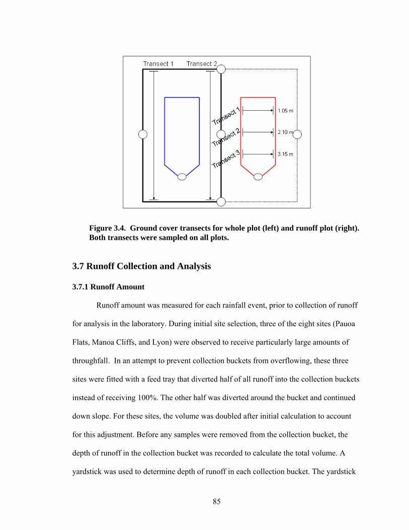
85
3.7 Runoff Collection and Analysis
3.7.1 Runoff Amount
Runoff amount was measured for each rainfall event, prior to collection of runoff
for analysis in the laboratory. During initial site selection, three of the eight sites (Pauoa
Flats, Manoa Cliffs, and Lyon) were observed to receive particularly large amounts of
throughfall. In an attempt to prevent collection buckets from overflowing, these three
sites were fitted with a feed tray that diverted half of all runoff into the collection buckets
instead of receiving 100%. The other half was diverted around the bucket and continued
down slope. For these sites, the volume was doubled after initial calculation to account
for this adjustment. Before any samples were removed from the collection bucket, the
depth of runoff in the collection bucket was recorded to calculate the total volume. A
yardstick was used to determine depth of runoff in each collection bucket. The yardstick
Figure 3.4. Ground cover transects for whole plot (left) and runoff plot (right). Both transects were sampled on all plots.

86
was cleaned with paper towels after each use. Sterile latex gloves were worn at all times,
and changed prior to each new measurement.
2.7.2 Runoff Overflow Buckets
During the initial months of this study, it was recognized that runoff collection
buckets were in many cases too small to collect the total amount of runoff from certain
rainfall events. A small hole was drilled in the downslope edge of each collection bucket
and a length of rubber hose was inserted in the hole. The rubber hose was layed
downslope and inserted into another hole drilled into a larger plastic tub (the “overflow
bucket”). This overflow bucket captured extra runoff to a volume of 97.7 L. A yard stick
was used to record runoff overflow volume as above.
2.7.3 Runoff TSS Analysis
After the depth was recorded, the contents of the collection bucket were
thoroughly mixed with the yardstick and a runoff water sample was collected in an acid-
washed 500 mL bottle. Samples were taken back to the lab on ice and refrigerated before
analysis for total suspended solids (TSS). Total SS were measured by vacuum filtration
of 100 mL of sample. First a Whatman 5 filter paper (Whatman, Kent, United Kingdom)
was placed on a watch glass and weighed on an electronic balance. Samples were
homogenized and a 100 mL aliquot was extracted and poured onto filter paper placed on
a Buchner funnel attached to a 500 mL vacuum flask. Each filter paper and watch glass
were then placed into a 105oC oven and dried for 24 hours. Afterwards the filters were

87
weighed and the original weight was subtracted from the dry weight to calculate the TSS
in g L-1 (EPA, 1971).
3.7.3 Runoff Enterococci Analysis
After the depth was recorded, the contents of the collection bucket were
thoroughly mixed and a runoff water sample was taken in a sterile 100 mL IDEXX
container (IDEXX Laboratories, Westbrook, ME). Samples were taken to the laboratory
on ice, and then refrigerated until analysis, within 36 hours of sample collection. In the
lab, 100 mL of sample was transferred with a pipette using sterile, disposable tips, to a
new sterile container and mixed with Enterolert reagent. Samples were shaken by hand a
minimum of 40 times to ensure proper mixing. Samples were diluted when runoff
samples contained high levels of sediment, or if previous samples were found
Enterococci levels to be higher than 2,500 CFU. At least one duplicate was made per
sample per sampling event. A control sample consisting of 100 mL of DI water was also
processed according to the same methods.
After mixing, samples were poured into labeled Quanti-Tray 2000 trays. The trays
were heat sealed and placed into a 41oC incubator for 24-28 hours. After incubation,
samples were removed and placed under an ultraviolet light to count the number of
fluorescing wells. Wells were counted only if fluorescence was complete (only brightest
wells were counted as positive). To determine Most Probable Number (MPN) of CFU,
the IDEXX Quanti-Tray MPN sheet was used. MPN for 90% dilutions was multiplied by
a factor of 10. MPN for 99% dilutions was multiplied by a factor of 100.

88
3.8 Enterococci in Soils
Surface soil samples were taken in August 2009 from each of the 14 plots and
analyzed for Enterococci. Soils were sampled with disposable plastic food-grade spoons
to ensure no cross contamination between plots. An aggregate sample was prepared from
four locations within each plot, from the top 0-5 cm of soil surface, approximately 30 cm
from each corner of the runoff channelizing plot. Samples were stored in sterile
disposable Ziploc bags and transported on ice to the laboratory. Enterococci analysis
methods were based on recommended USGS techniques (Myers et al., 2007) and Ragosta
(2007). Approximately 5 g of soil was weighed and placed in a sterile IDEXX bottle. One
hundred mL of sterile 0.15 M NaCl dispersant solution was added to the sample. Sample
bottles were then placed on a rotary shaker table for 45 minutes.
After shaking, samples were left to settle for 30 seconds then a 10 mL aliquot was
removed from the top 30-40% of solution by sterile pipette and transferred to a new
sterile IDEXX bottle. 90 mL of sterile DI water was added along with the Enterolert
reagent. Samples were placed on a shaker table for another 5 minutes. After the final
shaking, samples were then heat sealed in Quanti-Tray 2000 trays and processed identical
to the methods described in section 3.7.3.
3.9 Statistical Analyses
All statistic analyses were performed using SAS version 9.1 (SAS Institute, Cary,
NC). A GLM ANOVA was used to investigate differences in variables that were only
measured once such as ground cover and soil Enterococci among sites. For the GLM
ANOVAs, a post-hoc comparison of means was carried out using Duncan’s Multiple

89
Range Test. A repeated measures ANOVA was used to differentiate between Enterococci
levels in among months and sites, and in fenced versus unfenced treatments. Month was
the repeated factor in these analyses. A least squares procedure was used for post-hoc
mean comparisons. Spearman correlation was used to evaluate relationships among
Enterococci and all environmental variables. A multiple stepwise regression (MSR) was
also used to determine the best predictors of Enterococci in runoff.
Results
3.10 Enterococci in Runoff
Enterococci levels in runoff were highly variable, ranging from <1 cfu 100 mL-1
to >72,000 CFU 100 mL-1 for individual measurements. The average level of Enterococci
in runoff was 6620.5 CFU 100 mL-1. The repeated measures ANOVA indicated that
month, site, and the month by site interaction accounted for a significant proportion of the
variance in the Enterococci data (Table 3.2). Treatment, while not significant at α =0.05,
was significant at α = 0.1.
Table 3.2. Repeated Measures ANOVA model for Enterococci levels in runoff. Source
Num df
Den df
Chi- Square
F-statistic
p-value
Month 10 60 213.86 21.39 <.0001 Site 6 60 65.52 10.92 <.0001 Treatment 1 60 2.90 2.90 0.094 Month x Site 60 60 166.14 2.77 <.0001 Month x Treatment 10 60 14.11 1.41 0.20 Site x Treatment 6 60 1.34 0.22 0.97
October and December had significantly higher Enterococci levels than any other
month, though they were the third and fourth largest rain events, respectively. October

90
and December had more than twice the Enterococci CFU, on average, than any other
month. The other months were all statistically similar. December, as well as having the
highest mean Enterococci levels, also had the largest rain event and the highest TSS
levels. June, September, and March had the lowest Enterococci levels, with <1,000 CFU
100 mL-1 average in runoff (Figure 3.5). The data shows a seasonal trend with the three
months having the highest Enterococci levels sequentially in October, November, and
December.
0
5000
10000
15000
20000
25000
30000
35000
June Ju
ly
Augus
t
Septe
mbe
r
Octob
er
Novem
ber
Decem
ber
Janu
ary
Febru
ary
Mar
chApr
il
En
tero
co
cc
i (C
FU
)
Enterococci in runoff were, on average, highest at Manoa Cliffs and lowest at
Waahila Ridge (Figure 3.6). Manoa Cliffs had significantly higher mean Enterococci in
runoff than only Pauoa Flats and Waahila Ridge. Pauoa Flats had the highest mean TSS
in runoff, and yet had the second-lowest mean Enterococci in runoff as well as in soil
samples. Waahila Ridge had the lowest mean Enterococci in runoff, as well as the lowest
mean throughfall and lowest mean runoff among all sites.
Figure 3.5. Mean Enterococci levels in runoff per month averaged across all sites. Error bars represent ± 1 standard error. Letters indicated significant difference according to least squared means.
A
B
B
B
B B
A
B B
B
B

91
0
2000
4000
6000
8000
10000
12000
14000
16000
LY MC MF PF PP RT WR
En
tero
co
cc
i (C
FU
)
The fenced and unfenced treatment means showed a significant difference at
α=0.1 (Figure 3.7). The fenced plots averaged 6,248 CFU 100 mL-1, while the unfenced
plots average 6,326 CFU 100 mL-1.
fenced unfenced0
1000
2000
3000
4000
5000
6000
7000
8000
9000
10000
En
tero
co
cc
i (C
FU
)
Figure 3.7. Mean Enterococci levels in fenced versus unfenced plots averaged across all months and sites. Error bars represent ± 1 standard error.
Figure 3.6. Mean Enterococci levels in runoff per site averaged across all month. Error bars represent ± 1 standard error. Letters indicate significantly different means according to least squared means.
A
AB
B
AB
AB B
AB
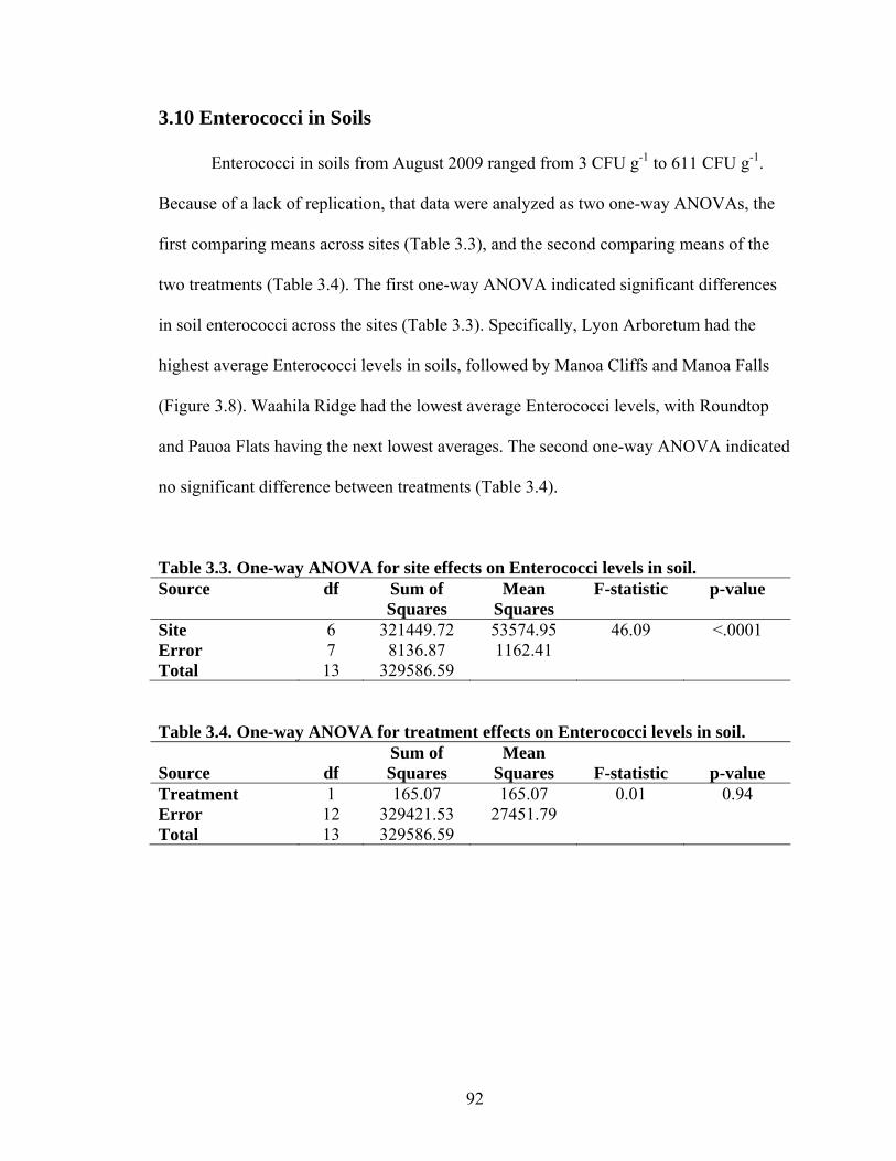
92
3.10 Enterococci in Soils
Enterococci in soils from August 2009 ranged from 3 CFU g-1 to 611 CFU g-1.
Because of a lack of replication, that data were analyzed as two one-way ANOVAs, the
first comparing means across sites (Table 3.3), and the second comparing means of the
two treatments (Table 3.4). The first one-way ANOVA indicated significant differences
in soil enterococci across the sites (Table 3.3). Specifically, Lyon Arboretum had the
highest average Enterococci levels in soils, followed by Manoa Cliffs and Manoa Falls
(Figure 3.8). Waahila Ridge had the lowest average Enterococci levels, with Roundtop
and Pauoa Flats having the next lowest averages. The second one-way ANOVA indicated
no significant difference between treatments (Table 3.4).
Table 3.3. One-way ANOVA for site effects on Enterococci levels in soil. Source df Sum of
Squares Mean
Squares F-statistic p-value
Site 6 321449.72 53574.95 46.09 <.0001 Error 7 8136.87 1162.41 Total 13 329586.59 Table 3.4. One-way ANOVA for treatment effects on Enterococci levels in soil. Source
df
Sum of Squares
Mean Squares
F-statistic
p-value
Treatment 1 165.07 165.07 0.01 0.94 Error 12 329421.53 27451.79 Total 13 329586.59

93
0
100
200
300
400
500
600
LY MC MF PF PP RT WR
CF
U/g
so
il
While the treatment effect was not significant, Enterococci levels were slightly higher in
soils of unfenced (124.7 CFU g-1) versus fenced plots (131.5 CFU g-1) (Figure 3.9).
Fenced Unfenced0
20
40
60
80
100
120
140
160
180
200
En
tero
co
cci
(c
fu)
Figure 3.9. Mean soil Enterococci levels in fenced versus unfenced plots in colony forming units g-1 dry weight soil,. Error bars represent ± 1 standard error.
Figure 3.8. Mean Enterococci levels in soils across sites in August 2009 in colony forming unit g-1 dry weight soil. Error bars represent ± 1 standard error. Letters indicate significantly different means according to least squared means.
A
C
B
BC
C
BC
C

94
There was also a trend of the sites with the greatest occurrence of pig disturbance having
more Enterococci in soils of the unfenced plots (Figure 3.11). For example, Puu Pia had
higher average levels in the unfenced (114 CFU g-1) than the fenced plot (14 CFU g-1).
Roundtop had higher Enterococci levels in the unfenced (39 CFU g-1) than the fenced (20
CFU g-1).
0
100
200
300
400
500
600
700
LY MC MF PF PP RT WR
CF
U/g
so
il
Fenced
Unfenced
3.16 Correlation of Enterococci with Environmental Variables
The only variables that had significant Spearman correlations with Enterococci in
runoff were runoff amount, runoff-throughfall ratio (RTR), and soil Enterococci from
Aug. 2009. The strongest correlation of Enterococci in runoff was with Enterococci in
soils (r = 0.74, p = 0.0024). Enterococci levels in runoff and soils were positively
correlated, yet neither was correlated with TSS or soil moisture. Throughfall, soil
moisture, and bare soil cover were thought to perhaps be important environmental
Figure 3.11. Mean Enterococci levels in soils among fenced versus unfenced plots across all sites. Error bars represent ± 1 standard error.

95
predictors of Enterococci in runoff, however none of these variables were significant
even at α = 0.1.
Soil Enterococci was also positively correlated with runoff amount, RTR, and
rock cover. Runoff amount had the highest Spearman correlation with Soil Enterococci (r
= 0.67, p = 0.0081), which was stronger than the correlation of runoff amount with
Enterococci in runoff. Soil Enterococci was correlated with throughfall, though only at
93% significance (r = 0.50, p = 0.071). Soil Enterococci was not significantly correlated
with soil moisture or soil carbon.
The correlation of Enterococci in runoff with environmental variables were also
tested separately for dry season and wet season months. During the dry season, none of
the environmental variables except RTR were significantly correlated with Enterococci in
runoff. Dry season Enterococci in runoff were negatively correlated with RTR, while
overall and in the wet season they were positively correlated. Runoff-throughfall ratio
was negatively correlated with dry season Enterococci in runoff. During the wet season,
Enterococci levels in runoff were significantly correlated with runoff amount, RTR, and
soil Enterococci.
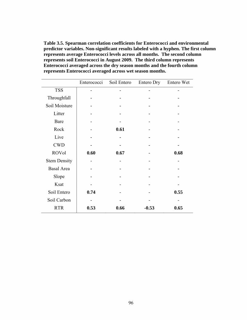
96
Table 3.5. Spearman correlation coefficients for Enterococci and environmental predictor variables. Non-significant results labeled with a hyphen. The first column represents average Enterococci levels across all months. The second column represents soil Enterococci in August 2009. The third column represents Enterococci averaged across the dry season months and the fourth column represents Enterococci averaged across wet season months.
Enterococci Soil Entero Entero Dry Entero Wet
TSS - - - -
Throughfall - - - -
Soil Moisture - - - -
Litter - - - -
Bare - - - -
Rock - 0.61 - -
Live - - - -
CWD - - - -
ROVol 0.60 0.67 - 0.68
Stem Density - - - -
Basal Area - - - -
Slope - - - -
Ksat - - - -
Soil Entero 0.74 - - 0.55
Soil Carbon - - - -
RTR 0.53 0.66 -0.53 0.65

97
Soil Enterococci and runoff volume were selected as important predictor variables
and entered into a multiple-stepwise regression. The runoff-throughfall ratio was not
selected as an important predictor variable because of the direct relationship with runoff
volume. At the α = 0.05 level no model was significant so α was raised 0.1. Runoff
amount then became a significant predictor of Enterococci in runoff (r = 0.49, p = 0.067).
Equation 2. Model for predicting Enterococci in runoff, based on multiple-stepwise regression (r2 = 0.27, p = 0.056).
3.12 Discussion
The first objective of this chapter was to quantify Enterococci in runoff and soils
from forested areas of the Manoa watershed. Previous research has suggested that
Enterococci are free-living and reproduce in the moist, warm environment of subtropical
islands such as Hawaii, Guam, and Puerto Rico (Fujioka et al., 1999; Byappanahalli and
Fujioka, 2004; Hartel et al., 2005), and these results partially agreed with their findings.
Every site contained Enterococci in runoff during multiple rain events, regardless of the
fenced or unfenced treatment. The exclusion fences had been in place over one year at the
start of the study, so soils were free of pig influence for at least that amount of time. The
Manoa Cliffs site had the highest Enterococci levels in runoff, despite fairly low levels of
TSS, averaging 10,072 CFU 100 mL-1. Pig rooting was observed several times at this site
and pig disturbance of the unfenced runoff plot was confirmed on multiple occasions by
game cameras. At this site the unfenced plot averaged almost 1,400 CFU 100 mL-1 more
than the fenced plot. The least amount of Enterococci in runoff occurred at the site with
Enterococci = 2526.69 + 519.30(RO Volume)

98
the lowest throughfall and lowest TSS levels: Waahila Ridge. Waahila Ridge was another
site where pig rooting evidence was seen in the unfenced plot, and Enterococci levels
were, on average, almost three times as high in the unfenced treatment compared to the
fenced treatment (4,756 100 mL-1 versus 1,204 CFU 100 mL-1).
Some commonality in the data for runoff and for soils was the high monthly and
intersite variability. The coefficient of variation (CV) ranged from 1.0-2.1 for individual
sites between months. Measurements showed high variability in Enterococci levels. Even
between duplicate samples, there were large amounts of variation; CVs ranging from 0.2-
1.2 among the sites. Enterococci levels in soil were standardized per gram of dry-weight
soil. On occasion there was even one order of magnitude difference between duplicate
samples (from Manoa Falls and Manoa Cliffs in April runoff event; Manoa Cliffs, Manoa
Falls, and Waahila Ridge soils) a result that was also found by Hartel et al. (2005) in a
study of Enterococci in coastal sediments and runoff. That study also investigated the
occurrence of false positives in Enterolert wells, finding that such artificial flourescences
resulted in decreases between the original and corrected MPN ranging from 0 to >99.9%.
Hartel et al. (2005) concluded that “the Enterolert system should be used with caution in
waters containing high amounts of sediment” which may be seen as a warning against
future use of the method in runoff and soil samples. However they also noted that, in their
opinion, there is not a better alternative to Enterococci as fecal indicator bacteria. They
proposed that care should be taken not to disturb the sediment when sampling water for
fecal contamination, or if the sediment is already disturbed (for instance on windy days or
when sampling runoff), then “the influence of sediment should be considered.”

99
The second objective was to determine whether feral pigs increase Enterococci
levels in runoff and soils. This objective was difficult to accomplish because of the
previously mentioned variability and potential for false positives. The inter-site and
temporal variability appeared to have greater influence on runoff amounts and
composition than did pig exclusion. However, the pig exclusion fencing treatment
showed a significant difference at α=0.1, suggesting that feral pigs increase Enterococci
in runoff. In an exclusion fencing study, Doupé et al. (2009) found that feral pigs
disturbed sediments in unfenced wetlands, affecting turbidity, pH, and anoxia; though
they also found that temporal effects had a greater influence on the environmental
variables measured than did the pigs. There were other interesting trends that developed
in the data, with higher Enterococci in soils and runoff from unfenced plots at certain
sites with higher occurrence of pig disturbance.
The increase in Enterococci may suggest fecal contamination. However, the use
of Enterococci as an indicator of fecal contamination is a contentious subject, particularly
in tropical and subtropical environments. Soil, water, and even plants are thought to be
reservoirs or sources of Enterococci (Mundt, 1961; Fujioka, 1999; Byappanahalli and
Fujioka, 2004). Fujioka in particular has intimated that Enterococci are not an ideal fecal
indicator in Hawaii and other tropical environments. Ragosta (2007) takes an opposing
view, believing Enterococci are valuable in Hawaii as an indicator of fecal contamination
and disturbance of exotic animals. Ragosta (2009) has also shared personal data, gathered
while working for the Koolau Mountain Watershed Partnership, from difficult to access,
high altitude areas of Oahu that showed little or no Enterococci presence. This data

100
indicates that Enterococci are not ubiquitous in Hawaiian soils, and are associated with
feral animals or even human activities.
The data from this study suggested that feral pigs may increase Enterococci in
runoff. Feral pig rooting could be increasing Enterococci in runoff by disturbing soils and
Enterococci already present in the soils. However, TSS was not significantly different
between fenced and unfenced treatments; therefore, it seems more likely that the increase
in Enterococci is coming directly from the pigs themselves. This is an important result
because although Enterococci are not themselves dangerous, feral pigs have been shown
to be reservoirs for human pathogens (Hampton et al., 2006). Research has also found
that Enterococci in surface waters correlate with incidence of sickness in bathers (Wade,
2006).
The third objective was to investigate temporal and spatial differences in
Enterococci presence in runoff. The data showed that Enterococci levels measured in
runoff and soils were temporally and spatially variable, differing greatly across sites and
months as evidenced by the month by site interaction. Enterococci in runoff ranged by
many orders of magnitude from <1 CFU 100 mL-1 during many of the smaller runoff
events, to >70,000 CFU 100 mL-1 from the Lyon Arboretum fenced site during the
December event. Similarly high variability was found by Hartel et al. (2005) in their
study of sediments from Georgia, New Hampshire, and Puerto Rico. October and
December had significantly higher Enterococci levels than any other months. Though
December was the largest runoff event, and Enterococci in runoff were found to correlate
with runoff amount, October was the third-smallest runoff event. October is a month

101
when strawberry guava (P. cattleainum), a food source of feral pigs, is fruiting in many
parts of the watershed, and several of the sites are near large strawberry guava stands.
While month and site accounted for a significant proportion of the variance in the
Enterococci levels in runoff, the month by site interaction was also significant. In general,
Manoa Cliffs and Manoa Falls had the two highest average Enterococci levels, and both
sites also showed evidence of pig disturbance on multiple occasions; however, Lyon
Arboretum had the next highest levels despite a lack of evidence of pig presence. This is
not to say pigs were never present at the Lyon Arboretum site, but the Arboretum does
encourage hunting, and has even set up a pig blind in an area several hundred yards
upslope from the runoff plots. The site did show higher averages in the unfenced plot
however, and Arboretum employees indicated that many rats live in the area. Manoa
Cliffs, Manoa Falls, and Lyon Arboretum also have high throughfall levels, but another
site with high throughfall levels, Pauoa Flats, had the second lowest Enterococci levels in
runoff.
Quantification of Enterococci in soils was accomplished in August 2009, though
it required a more extensive analysis process than the runoff. The Lyon site contained the
highest levels of Enterococci in soils, averaging 476 CFU g-1; this was more than double
the level of any other site, but lower than levels found in sediments from Georgia, New
Hampshire, and Puerto Rico (Hartel et al., 2005). Just as with the runoff Enterococci,
Waahila Ridge showed the lowest soil Enterococci levels, averaging 24 CFU g-1. This
range is similar to Hartel et al. (2005) where Enterococci numbers occasionally exceeded
1,000 g-1 of soil, but frequently were as low as 10 g-1, when present. In a study in the
Waipa watershed on the northern side of the island of Kauai, Ragosta (2007) found a
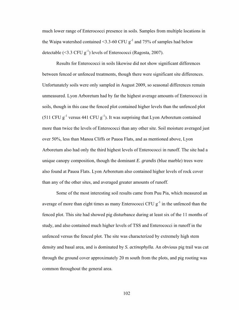
102
much lower range of Enterococci presence in soils. Samples from multiple locations in
the Waipa watershed contained <3.3-60 CFU g-1 and 75% of samples had below
detectable (<3.3 CFU g-1) levels of Enterococci (Ragosta, 2007).
Results for Enterococci in soils likewise did not show significant differences
between fenced or unfenced treatments, though there were significant site differences.
Unfortunately soils were only sampled in August 2009, so seasonal differences remain
unmeasured. Lyon Arboretum had by far the highest average amounts of Enterococci in
soils, though in this case the fenced plot contained higher levels than the unfenced plot
(511 CFU g-1 versus 441 CFU g-1). It was surprising that Lyon Arboretum contained
more than twice the levels of Enterococci than any other site. Soil moisture averaged just
over 50%, less than Manoa Cliffs or Pauoa Flats, and as mentioned above, Lyon
Arboretum also had only the third highest levels of Enterococci in runoff. The site had a
unique canopy composition, though the dominant E. grandis (blue marble) trees were
also found at Pauoa Flats. Lyon Arboretum also contained higher levels of rock cover
than any of the other sites, and averaged greater amounts of runoff.
Some of the most interesting soil results came from Puu Pia, which measured an
average of more than eight times as many Enterococci CFU g-1 in the unfenced than the
fenced plot. This site had showed pig disturbance during at least six of the 11 months of
study, and also contained much higher levels of TSS and Enterococci in runoff in the
unfenced versus the fenced plot. The site was characterized by extremely high stem
density and basal area, and is dominated by S. actinophylla. An obvious pig trail was cut
through the ground cover approximately 20 m south from the plots, and pig rooting was
common throughout the general area.

103
The final objective of this study was to investigate correlations between
environmental variables and Enterococci in runoff. This was accomplished, though the
some of the results were unexpected. Of the 14 environmental variables recorded, only
runoff volume and soil Enterococci significantly correlated with Enterococci in runoff.
The positive correlation with runoff volume could result because larger runoff events also
may correlate with higher intensity throughfall events, and therefore may be more likely
to disturb Enterococci from soils and other surfaces. The positive correlation of
Enterococci in runoff with Enterococci in soils seems obvious; sites with more
Enterococci in soils would likely have more Enterococci in runoff. It was surprising that
there were no other significant correlations in the data. The lack of correlation with soil
moisture was surprising, as wet soils were thought to be more accommodating to survival
of the bacteria (Cools et al., 2001; Hartel et al., 2005). Likewise, the lack of correlation
with TSS was also unexpected. Bacteria are known to associate with sediment particle
surfaces, and sediments in water protect bacteria from environmental conditions that
could be hazardous to their survival (Anderson et al., 2005). Soil carbon levels measured
at the seven sites by Browning (2008) were significantly correlated with soil moisture,
basal area, and slope but had no relationship with Enterococci in runoff or soils.
3.13 Conclusions
Hypothesis one predicted that Enterococci levels in runoff would be higher in the
wet season (November-April) than dry season (May-October). The data did not support
this hypothesis, as a month by site interaction indicated that seasonal (monthly) trends
were not consistent across the sites. In general, October and December had significantly

104
higher Enterococci levels in runoff than the other months, both averaging >20,000 CFU
100 mL-1. Both months had larger than average runoff events, which may relate to the
correlation of Enterococci with runoff amount.
Hypothesis two predicted that Enterococci levels in runoff and soil would be
increased by the presence of feral pigs. This was partially supported by the data.
Unfenced versus fenced comparisons of runoff showed a significant (α = 0.1) difference
in Enterococci levels. There were higher average Enterococci levels in unfenced plots in
both soils and runoff from several sites, such as Puu Pia, Waahila Ridge, and Roundtop;
the sites with highest recorded pig disturbance. However, fenced plots also showed high
levels of Enterococci in runoff and soils. Several factors could explain this result. First is
the potential presence of rats (Rattus spp.) and/or mongoose (Herpestes javanicus) inside
the fenced plots. At Roundtop in particular, avocado fruits that fell inside the fenced plot
were seen to be partially eaten, and tooth marks were evident in the flesh. Both of these
animals are potential vectors for Enterococci, and both could presumably access the
fenced plot.
Hypothesis three predicted that of all environmental predictors, ground cover and
soil moisture would have strongest correlation with Enterococci in runoff. Ground cover
was thought to correlate with pig disturbance, and soil moisture was thought to allow for
greater chance of Enterococci survival in soils. The data did not support this hypothesis
as Enterococci in runoff were significantly correlated with runoff volume and with
Enterococci in soils, but not with soil moisture or any of the ground cover variables.
Enterococci in soils were significantly correlated with the percent cover of rock in the
runoff plots. This result was unexpected, and there does not seem to be a logical reason

105
for such a relationship. Moist soils were expected to be more conducive to bacterial
growth (Anderson et al., 2007), but this relationship was not found. This suggests that
some other factors are responsible, and more research is needed on Enterococci levels in
surface waters and soils in Hawaiian watersheds.
Hypothesis four stated that TSS in runoff would positively correlate with
Enterococci abundance in runoff. This hypothesis was also not supported by the data.
Enterococci in runoff did not significantly correlate with TSS. It was expected that
Enterococci would be present in soils, and as sediment levels in runoff increased so
would levels of Enterococci. This result was not seen, and it could be that the bacteria are
more prevalent on the ground surface, and therefore are carried in runoff regardless of
sediment disturbance. Though Enterococci were present in soils, the levels were
relatively low, and as mentioned in section 3.16, they were less than the upper limits of
levels seen in studies of sediments from areas on the continental U.S. This may suggest
that Enterococci are associated with animals and deposited on litter, rocks, plants, and the
soil surface. Birds are known to be a major source of Enterococci contamination at
beaches (Haack et al., 2003), and could have deposited these bacteria inside both fenced
and unfenced areas.
Comparative studies of fencing to exclude feral pigs or inhibit their access into
sensitive forested areas are few (Campbell and Long, 2009), and these runoff plots
provide an excellent opportunity to study feral pig impacts on water quality, soils, and
vegetation. Other than previous research at these same runoff plots (Browning, 2008), no
other study has been found to use runoff plots and exclusion fencing in the upper forested
areas of a watershed. In addition to elucidating monthly and site differences in runoff and

106
their interactions, this research provides baseline conditions for further research at the
runoff plots. As time goes on, differences between fenced and unfenced plots are
expected to continue to develop, and further research is needed at these sites.

107
CHAPTER 4: CONCLUSIONS
This study was designed to elucidate the runoff dynamics and processes occurring
in the upper forested areas of a Hawaiian watershed and the effects of feral pigs on water
quality and fecal indicator bacteria. The large amount of runoff captured from some of
these plots was an unexpected result. The high levels of TSS in runoff were also an
important finding. These high levels of TSS in runoff were more likely in the wet season
and from certain areas in the watershed, particularly Puu Pia, Pauoa Flats, and Lyon
Arboretum. These were high throughfall sites, which were mostly dominated by
nonnative vegetation. Total SS in runoff was predicted by soil moisture, throughfall , and
coarse woody debris cover. While the Manoa Cliffs site had high throughfall, it also had
the most native vegetation, and had correspondingly low TSS levels. This research
suggests that TSS levels in runoff are of more concern during the wet season, from
certain areas in the upper watershed.
While Enterococci in runoff were found to be significantly higher in unfenced
plots at α=0.1, they were also highly variable among months and sites. The data suggests
that other factors such as location, animal presence, or soil type may be important in
influencing Enterococci levels in runoff. Enterococci levels were also significantly
correlated with runoff volume and with Enterococci levels in soils. Enterococci were
present in soils from all sites tested, but at levels similar to those seen in studies of
sediments from areas in the continental U.S. There were higher average Enterococci
levels in unfenced plots in both soils and runoff from several sites, such as Puu Pia,
Waahila Ridge, and Roundtop; the sites with the highest recorded levels of pig

108
disturbance.
Effects of pig disturbance on runoff and soils were difficult to elucidate. Certain
sites that showed high amounts of pig rooting and disturbance evidence, in particular Puu
Pia and Waahila Ridge, had greater levels of TSS from unfenced plots. Enterococci in
runoff and Soil Enterococci were also higher in unfenced plots from Puu Pia and Waahila
Ridge. Psidium cattleianum is known to be spread by feral pigs, and seedlings and
sapling counts were higher in unfenced plots. Bare ground cover was on average higher
in the unfenced than the fenced plots.
The only other study found to have a similar approach was previous research on
the same runoff plots (Browning, 2008). Besides elucidating monthly and site differences
in runoff and their interactions, this study provides baseline conditions for further
research at the runoff plots. As time goes on, I expect differences between fenced and
unfenced plots will continue to develop. The complexity of runoff processes and the
presence of other exotic animals in the study area present a problem when trying to study
solely the impacts of feral pigs. However, I believe this can be accomplished, and this
study has identified many ways to improve monitoring of runoff plots and feral pigs. The
presence of pigs is a divisive issue in many Hawaiian communities, pitting pig hunters
and residents who depend on the pigs for food against conservationists and others who
worry about the damage afflicted by these exotic mammals. Regardless of which side of
the debate one takes, it is of the utmost importance that the ecological and watershed
effects of feral pigs be understood.

109
4.1 Further Research
Comparative studies of fencing to exclude feral pigs or inhibit their access into
sensitive forested areas are few (Campbell and Long, 2009), and these runoff plots
provide an excellent opportunity to study feral pig impacts on water quality, soils, and
vegetation. More than two years have passed since exclusion fences were installed, and I
expect that differences between fenced and unfenced plots will become more pronounced
as time goes on. Soil organisms are a known indicator of disturbance (Vtorov, 1993), and
may respond to change quicker than other soil properties (Moody and Jones, 2000).
Analysis of soil organisms, and other soil properties such as pH, nutrients, and bulk
density could be important in determining pig impacts.
The research sites encompass a great variety in vegetation and canopy structure,
with 14 different canopy tree species, and at least 21 total different woody plant species.
The difference in P. cattleianum seedlings between fenced and unfenced sites highlighted
the potential impacts of feral pigs on vegetation and forest structure. Though the fenced
areas are small, this study has provided a necessary baseline to continue conducting
research on vegetation differences between plots; particularly with regard to exotic
fruiting trees such as P. cattleianum and Persea americana.
The deployment of game cameras midway through the study proved that feral
pigs did access several of the unfenced plots. Further research with game cameras could
allow for estimation of pig populations and shed light on the behavior of these secretive
and shy mammals. Using camera trapping rate is a promising and cost-effective for the
rapid assessment of animal abundance in remote areas or where alternative methods are
unfeasible (Rovero and Marshall, 2009). Camera trapping has the potential to simplify

110
data collection and reduce human error that can be a problem in other abundance survey
methods.
Though pigs were conclusively seen to visit several of the sites, only at Waahila
Ridge was extensive rooting seen inside the runoff plot. One potential avenue for further
research would be to lure pigs to the plots. Bananas or other fruit could be spread
throughout each unfenced area, encouraging the pigs to spend more time inside the
unfenced runoff plots. Thus, the effects on runoff and soils could become more
pronounced. Though this could artificially increase pig effects at the runoff, nonnative
fruit trees are common throughout many Hawaiian wet forests so such disturbance may
not be unusual in areas of the watershed.
4.2 Recommendations for Improvement
Considering the large amounts of runoff, and the problem of exceeding bucket
capacity, I would recommend that overflow buckets be installed at every site to better
quantify runoff amounts. Collection splitters could also be deployed at every site. Lyon
Arboretum exceeded the overflow bucket capacity on several occasions; therefore larger
overflow buckets may also be needed. Perhaps an automated system could be used that
measured total runoff without having to store the entire amount. Another area of missing
data is throughfall intensity. This is an important factor in runoff generation, and the
throughfall gauges used in this study did not provide any information on intensity of
throughfall events. A tipping-bucket or similar throughfall gauge installed at each site
would be a valuable addition to further studies.

111
The game cameras provided indisputable evidence that pigs are present at certain
sites. Installation of cameras at every site would allow for a better understanding of pig
movements and permit comparison of pig presence/populations among sites. Ground
cover was measured at the closing stages of this study but I would recommend that any
further research entail ground cover estimation at the outset as well, to allow for more
robust analysis of pig effects on ground cover. Canopy cover is an environmental variable
potentially very important for runoff processes. Canopy cover above each site could be
estimated with a LAI-2000 or other such device to aid in better understanding runoff
processes in these forested areas.
The data suggested a difference between fenced and unfenced treatments for
Enterococci in runoff. There were no statistically significant differences seen in TSS in
runoff or ground cover. A potential problem with drawing conclusions from this type of
study is the proximity of the runoff plot to the fence. Exclusion fences may alter pig
behavior and impede normal movements, magnifying pig effects (Noguiera-Filho et al.,
2009). If additional runoff plots are added to the study, a larger separation between
fenced and unfenced plots may be advisable to avoid a bias in ground cover and soils
measurements.
Finally, I believe a second method for enumerating Enterococci should be used to
confirm the accuracy of the IDEXX method. As mentioned in section 3.18, literature has
been published that brings into question the reliability of this method, particularly when
testing water samples containing high levels of sediment, which runoff often does. Since
Enterococci is still an accepted water quality indicator according to the US EPA, this
would be an important addition to further research involving Enterococci.

112
APPENDIX A: TREE SPECIES LISTS
Table 4. List of canopy tree species at Lyon Arboretum. Species Count Ficus microcarpa (Chinese banyan) 48 Elaecarpus grandis (blue marble) 17 Unknown #2 7 Dracaena sp. (money tree) 2 Livistona chinensis (Chinese fan palm) 2
Table 5. List of canopy tree species at Manoa Cliffs. Species Count Hibiscus arnottianus (kokio keokeo) 62 Cestrum nocturnum (night-blooming jasmine) 34 Cinnamomum burmanni (Indonesian cinnamon) 13 Pisonia umbellifera (pepala kepau) 7 Psidium guajava (common guava) 7 Cordyline fruticosa (ti) 6 Ardisia elliptica (shoebutton Ardisia) 6
Table 6. List of canopy tree species at Manoa Falls. Species Count Psidium cattleianum (strawberry guava) 197 Unknown #8 5 Ficus microcarpa (Chinese banyan) 3 Cinnamomum burmanni (Indonesian cinnamon) 1 Unknown #7 1

113
Table 7. List of canopy tree species at Pauoa Flats. Species Total Cinnamomum burmanni (Indonesian cinnamon) 42Elaecarpus grandis (blue marble) 7Ardisia elliptica 3Unknown #7 3Ficus microcarpa (Chinese banyan) 2Schefflera actinophylla (octopus tree) 1
Table 8. List of canopy tree species at Puu Pia. Species Count Schefflera actinophylla (octopus tree) 333 Eucalyptus robusta (swamp mahogany) 35 Ardisia elliptica (shoebutton Ardisia) 3 Psidium cattleianum (strawberry guava) 1
Table 9. List of canopy tree species at Roundtop. Species Count Schefflera actinophylla (octopus tree) 67 Livistona chinensis (Chinese fan palm) 13 Persea americana (avacado) 8 Psidium cattleianum (strawberry guava) 2 Cordyline fruticosa (ti) 2 Hibiscus tiliaceus (hau) 1
Table 10. List of canopy tree species at Waahila Ridge. Species Count Casaurina glauca (Ironwood) 146 Psidium cattleianum (strawberry guava) 38 Uknown #3 1

114
APPENDIX B: RUNOFF PLOT GROUND COVER MEASUREMENTS
0%
10%
20%
30%
40%
50%
60%
70%
80%
90%
100%
LYF LYU
Dead
CWD
Live
Root
Rock
Bare
Litter
0%
10%
20%
30%
40%
50%
60%
70%
80%
90%
100%
MCF MCU
Dead
CWD
Live
Root
Rock
Bare
Litter
Figure 5. Manoa Cliffs ground cover, fenced versus unfenced plot.
Figure 4. Lyon Arboretum ground cover, fenced versus unfenced plot.
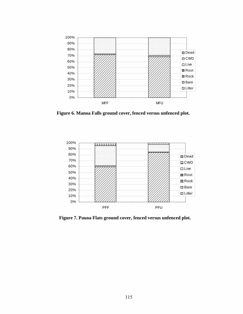
115
0%
10%
20%
30%
40%
50%
60%
70%
80%
90%
100%
MFF MFU
Dead
CWD
Live
Root
Rock
Bare
Litter
0%
10%
20%
30%
40%
50%
60%
70%
80%
90%
100%
PFF PFU
Dead
CWD
Live
Root
Rock
Bare
Litter
Figure 7. Pauoa Flats ground cover, fenced versus unfenced plot.
Figure 6. Manoa Falls ground cover, fenced versus unfenced plot.
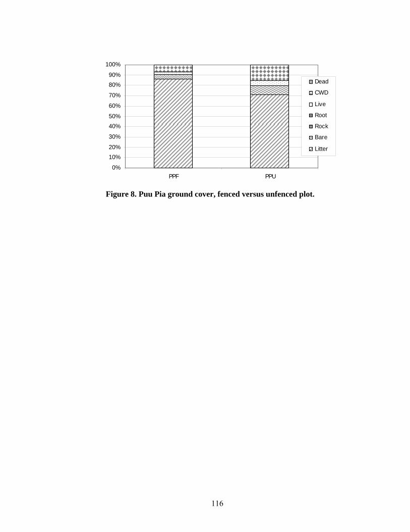
116
0%
10%
20%
30%
40%
50%
60%
70%
80%
90%
100%
PPF PPU
Dead
CWD
Live
Root
Rock
Bare
Litter
Figure 8. Puu Pia ground cover, fenced versus unfenced plot.

117
APPENDIX C: RAW DATA
Table 11. Enterococci, TSS, and runoff volume (ROVol) data from June 2008 through April 2009. Enterococci results in units of CFU 100 mL-1. TSS results in units of g L-1. Runoff volume results in units of liters. LY signifies Lyon Arboretum, MC signifies Manoa Cliffs, MF signifies Manoa Falls, PF signifies Pauoa Flats, PP signifies Puu Pia, RT signifies Roundtop, WR signifies Waahila Ridge. Site Treatment Month Enterococci TSS ROVolLY Fenced June 142.55 0.1 26.50048LY Unfenced June 217.6 0 26.50048MC Fenced June 0 0.1 2.864307MC Unfenced June 0 0.1 9.308998MF Fenced June 0 0 8.592922MF Unfenced June 236.05 0.1 8.95096PF Fenced June 1 0.1 0PF Unfenced June 0 0 0PP Fenced June 0 0.2 2.14823PP Unfenced June 0 0.1 2.864307RT Fenced June 0 0.3 2.864307RT Unfenced June 0 0.1 2.864307WR Fenced June 0 0 1.611173WR Unfenced June 0 0.1724138 1.790192LY Fenced July 6 0.05 5.370576LY Unfenced July 10.5 0.0980392 2.864307MC Fenced July 0 0 0.358038MC Unfenced July 0 0 1.432154MF Fenced July 3795.8 0.05 1.790192MF Unfenced July 412.6 0.125 4.47548PF Fenced July 0 0 0PF Unfenced July 0 0 0PP Fenced July 22 0.1 2.685288PP Unfenced July 4164.2 0.126 3.580384RT Fenced July 24196 0.092 1.969211RT Unfenced July 24196 0.15 2.14823WR Fenced July 24196 0.15 2.506269WR Unfenced July 13.55 0.05 2.685288LY Fenced August 58.35 0.05 26.50048LY Unfenced August 37 0.05 26.50048MC Fenced August 168 0.05 5.728614MC Unfenced August 103 0.106 6.444691MF Fenced August 50.1 0.05 13.25024MF Unfenced August 156 0.125 13.25024PF Fenced August 0 0 0.716077PF Unfenced August 0 0 0PP Fenced August 82.9 0.1 6.265672

118
Site Treatment Month Enterococci TSS ROAmtPP Unfenced August 1 0.126 7.160768RT Fenced August 12099.5 0 3.938422RT Unfenced August 107 0 3.759403WR Fenced August 1341.3 0.15 2.506269WR Unfenced August 13091.15 0.05 2.685288LY Fenced September 118.05 0.6666667 26.50048LY Unfenced September 20.25 0.3666667 26.50048MC Fenced September 154 0 16.8278MC Unfenced September 14.5 0 17.54388MF Fenced September 48 0 13.25024MF Unfenced September 1093 0.2666667 13.25024PF Fenced September 0 0 0PF Unfenced September 0 0 0PP Fenced September 12 0.1666667 6.62371PP Unfenced September 1949.75 0.3666667 7.339787RT Fenced September 59.05 0 8.055864RT Unfenced September 1006.2 0 6.981749WR Fenced September 183.35 0.1666667 13.25024WR Unfenced September 5.5 0.5666667 8.771941LY Fenced October 24196 0.6 26.50048LY Unfenced October 24196 0.1 26.50048MC Fenced October 24196 0 2.864307MC Unfenced October 24196 0.4 9.308998MF Fenced October 24196 0 8.592922MF Unfenced October 24196 0.1 8.95096PF Fenced October 24196 0.2 0PF Unfenced October 3322.3 1.5 0PP Fenced October 6111.8 0.1 2.14823PP Unfenced October 24196 1 2.864307RT Fenced October 24196 0.1 2.864307RT Unfenced October 24196 0.2 2.864307WR Fenced October 8975.3 0 1.611173WR Unfenced October 24196 0 1.790192LY Fenced November 3358 1.5 26.50048LY Unfenced November 15248 0.9 26.50048MC Fenced November 8558 0.3 26.50048MC Unfenced November 13073 0.4 26.50048MF Fenced November 5649 0.1 13.25024MF Unfenced November 35895 0.4 13.25024PF Fenced November 1154 2 25.06269PF Unfenced November 1159 2.5 25.77876PP Fenced November 4082.5 1.3 13.25024PP Unfenced November 9813.5 2.1 13.25024RT Fenced November 14313 0.5 5.907634

119
Site Treatment Month Enterococci TSS ROAmtRT Unfenced November 576.5 0.3 4.296461WR Fenced November 10 0 3.222346WR Unfenced November 93.5 0.1 3.043326LY Fenced December 51200 2.95 26.50048LY Unfenced December 38700 5.35 26.50048MC Fenced December 57300 2.15 26.50048MC Unfenced December 50500 2.25 26.50048MF Fenced December 72700 0.79 13.25024MF Unfenced December 1273.5 0.35 13.25024PF Fenced December 610 3.95 26.50048PF Unfenced December 1371.5 2.75 26.50048PP Fenced December 8773 5.65 13.25024PP Unfenced December 5620.5 7.05 13.25024RT Fenced December 3920.5 0.05 13.25024RT Unfenced December 2320 0 10.02508WR Fenced December 0 0 7.518806WR Unfenced December 0 0.15 7.518806LY Fenced January 1313.5 2.75 26.50048LY Unfenced January 9800 2.25 26.50048MC Fenced January 673 1.25 26.50048MC Unfenced January 3237.5 1.05 26.50048MF Fenced January 4321.5 0.25 1.969211MF Unfenced January 206.5 0 1.790192PF Fenced January 1058.5 2.3 19.33407PF Unfenced January 755 0.8 26.50048PP Fenced January 132 0.2 13.25024PP Unfenced January 3736 0.4 9.308998RT Fenced January 130 0 0.716077RT Unfenced January 14433 0 0.179019WR Fenced January 10 0 1.611173WR Unfenced January 5 0 1.611173LY Fenced February 2393 0.05 26.50048LY Unfenced February 2227 0 26.50048MC Fenced February 944.5 0 8.234883MC Unfenced February 14833.5 0 26.50048MF Fenced February 4371 0 2.685288MF Unfenced February 6524 0 3.580384PF Fenced February 0 0 0PF Unfenced February 22029.5 0 0.716077PP Fenced February 3719.5 0.45 13.25024PP Unfenced February 7717 0.65 13.25024RT Fenced February 63 0 3.222346RT Unfenced February 1622 0.05 1.432154WR Fenced February 0 0.25 3.043326
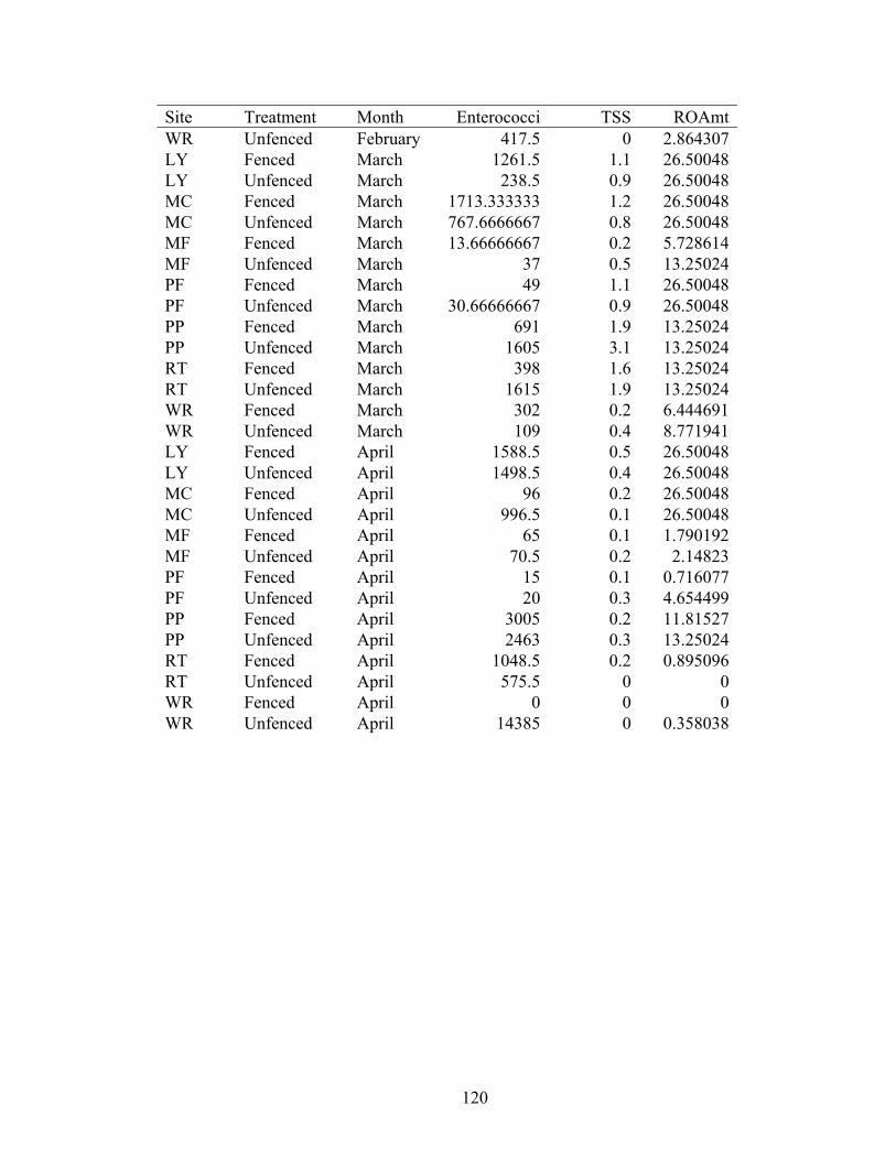
120
Site Treatment Month Enterococci TSS ROAmtWR Unfenced February 417.5 0 2.864307LY Fenced March 1261.5 1.1 26.50048LY Unfenced March 238.5 0.9 26.50048MC Fenced March 1713.333333 1.2 26.50048MC Unfenced March 767.6666667 0.8 26.50048MF Fenced March 13.66666667 0.2 5.728614MF Unfenced March 37 0.5 13.25024PF Fenced March 49 1.1 26.50048PF Unfenced March 30.66666667 0.9 26.50048PP Fenced March 691 1.9 13.25024PP Unfenced March 1605 3.1 13.25024RT Fenced March 398 1.6 13.25024RT Unfenced March 1615 1.9 13.25024WR Fenced March 302 0.2 6.444691WR Unfenced March 109 0.4 8.771941LY Fenced April 1588.5 0.5 26.50048LY Unfenced April 1498.5 0.4 26.50048MC Fenced April 96 0.2 26.50048MC Unfenced April 996.5 0.1 26.50048MF Fenced April 65 0.1 1.790192MF Unfenced April 70.5 0.2 2.14823PF Fenced April 15 0.1 0.716077PF Unfenced April 20 0.3 4.654499PP Fenced April 3005 0.2 11.81527PP Unfenced April 2463 0.3 13.25024RT Fenced April 1048.5 0.2 0.895096RT Unfenced April 575.5 0 0WR Fenced April 0 0 0WR Unfenced April 14385 0 0.358038

121
Literature Cited
Ahmed, W. (2005). “Host species-specific metabolic fingerprint database for enterococci and Escherichia coli and its application to identify sources of fecal contamination in surface waters.” Applied and Environmental Microbiology 71(8):4461-4468.
Allison, A. and S. E. Miller (2000). “Hawaii Biological Survey: Museum resources in support of conservation.” Nature and human society: The quest for a sustainable world. P. H. Raven and T. Williams. Washington D.C., National Academy Press: p. 281-290.
Anderson, K. L. J. E. Whitlock, and V. J. Harwood (2005). “Persistence and Differential Survival of Fecal Indicator Bacteria in Subtropical Waters and Sediments.” Applied and Environmental Microbiology 71(6):3041-3048.
Anderson, S., R. Hobdy and K. Maly (2007). “The need for more effective ungulate control in Hawaii.” White paper Haleakala National Park.
Anderson S.A., Turner S.J., and Lewis G.D. (1997). “Enterococci in the New Zealand environment: implications for water quality monitoring.” Water Science and Technology 35(11-12):325–331.
Atwill, E.R., R.A. Sweitzer, M. Das Grac¸ A. C. Pereira, I. A. Gardner, D. Van Vuren, W.M. Boyce (1997). “Prevalence of and Associated Risk Factors For Shedding Cryptosporidium parvum Oocysts and Giardia Cysts within Feral Pig Populations in California.” Applied and Environmental Microbiology. 63(10):3946–3949.
Borina, M., M. Vianello, F. Morari, G. Zanin (2005). “Effectiveness of buffer strips in removing pollutants in runoff from a cultivated field in North-East Italy.”
Agriculture, Ecosystems and Environment. 105:101–114. Browning, C.A. (2008). “A Preliminary Examination of the Effects of Feral Pigs (Sus
Scrofa) on Water Quality and Soil Loss Within a Hawaiian Watershed.” M.S. Thesis. University of Hawaii, Manoa. Department of Natural Resources and Environmental Management.
Byappanahalli M., and R. Fujioka (2004). “Indigenous soil bacteria and low moisture may limit but allow faecal bacteria to multiply and become a minor population in tropical soils.” Water Science and Technology 50(1):27-32.
Campbell, A. T., and D.B. Long (2009). “Feral swine damage and damage management in forested ecosystems. Forest Ecology and Management. 257:23319-2326.
Caley, P. (1993). “Population-Dynamics of Feral Pigs (Sus scrofa) in a Tropical Riverine Habitat Complex.” Wildlife Research. 20(5):625-636.
Cools, D., R. Merckxa, K. Vlassak, and J. Verhaegen (2001). “Survival of E. coli and Enterococcus spp. derived from pig slurry in soils of different texture.” Applied Soil Ecology 17 53–62.
Cooray, R. G. and D. Mueller-Dombois (1981). “Feral pig activity”. Island Ecosystems: Biological Organization in Selected Hawaiian Communities. Stroudsburg, Pennsylvania, Hutchinson Ross Publ. Co.: p. 309-317.
Cushman, J., T. Hall., A. Tierney, and J.M. Hinds (2004). “Variable effects of feral pig disturbances on native and exotic plants in a California grassland.” Ecological Applications. 14(6), p. 1746–1756.
De Carlo, E. H., D. J. Hoover, C. W. Young, R. S. Hoover, and F. T. Mackenzie(2007) “Impact of storm runoff from tropical watersheds on coastal water quality and

122
productivity.” Applied Geochemistry. 22:1777–1797. Donlan, J.C., K. Campbell, W. Cabrera, C. Lavoie, V. Carrion and F. Cruz (2007).
“Recovery of the Galápagos rail (Laterallus spilonotus) following the removal of invasive mammals.” Biological Conservation. 138(3):520-524.
Donlan, J.C. and C. Wilcox (2008). “Diversity, invasive species and extinctions in insular ecosystems” Journal of Applied Ecology. 45:1114–1123.
Doupe´, R. G., J. Mitchell, M. J. Knott, A. M. Davis, A. J. Lymbery (2009). “Efficacy of exclusion fencing to protect ephemeral floodplain lagoon habitats from feral pigs (Sus scrofa).” Wetlands Ecology and Management. Published online.
El-Swaify, S. (1989). “Monitoring of Weather, Runoff, and Soil Loss.” International Board for Soil Research and Management Inc. Soil Management and Smallholder Development in the Pacific Islands. IBSRAM Proceedings No. 8.
El-Swaify, S. A. (2000). “Operative Processes for Sediment-Based Watershed Degredation in Small, Tropical Volcanic Island Ecosystems.” Integrated Watershed Management in the Global Ecosystem. CRC Press LLC, Boca Raton, FL. 35-39.
EPA (1971). "EPA Method 160.2." EPA Test Methods. Retrieved June 15, 2008, from http://www.umass.edu/tei/mwwp/acrobat/epa160_2nonfiltres.pdf.
Fujioka R., C.Sian-Denton, and M.Borja, (1999). “Soil: the environmental source of Escherichia coli and enterococci in Guam's streams.” Journal of Applied Microbiology. 85:83-89.
Gersberg, R. M., M. A. Rose, R. Robles-Sikisaka, and A. K. Dhar (2006). “Quantitative Detection of Hepatitis A Virus and Enteroviruses Near the United States-Mexico Border and Correlation with Levels of Fecal Indicator Bacteria.” Applied and Environmental Microbiology. 72(12):7438–7444.
Glenn, C. R.; G. M McMurtry. (1995). “Scientific studies and history of the Ala Wai Canal, an artificial tropical estuary in Honolulu.” Pacific Science. 49(4):300- 318.
Grace, J. M. (2008). “Influence of Storm Characteristics on Soil Erosion and Storm Runoff.” ASABE Meeting Presentation. June 28-July 2.
Haack, S. K., L. R. Fogarty, and C. Wright (2003). “Escherichia coli and Enterococci at Beaches in the Grand Traverse Bay, Lake Michigan: Sources, Characteristics, and Environmental Pathways.” Environmental Science & Technology. 37 (15):3275- 3282.
Haile, R.W., J.S. Witte M., Gold, R. Cressey, C. McGee, R.C. Millikan, A. Glasser, N.Harawa, C. Ervin, P. Harmon, J. Harper, J. Dermand, J. Alamillo, K. Barrett, M. Nides, G.Y. Wang (1999). “The health effects of swimming in ocean water contaminated by storm drain runoff.” Epidemiology 10:355–63.
Hampton, J., P. B.S. Spencer, A. D. Elliot, and R.C. A. Thompson (2006). “Prevalence of Zoonotic Pathogens from Feral Pigs in Major Public Drinking Water Catchments in Western Australia.” EcoHealth 3:103–108.
Hardina, C.M. and R.S. Fujioka (1991) “Soil-the Environmental Source of Eschericia coli and Enterococci in Hawaii Streams.” Environmental Toxicology and Water Quality. 6 (2):185-195.
Hartel, P. G., K. Rodgers, J. A. Fisher, J. L. McDonald, L. C. Gentit, E. Otero, Y. Rivera Torres, T. L. Bryant, and S. H. Jones (2005). “Survival and Regrowth of Fecal

123
Enterococci in Desiccated and Rewetted Sediments.” Proceedings of the 2005 Georgia Water Resources Conference.
Hone, J. (2002). “Feral pigs in Namadgi National Park, Australia: dynamics, impacts and management.” Biological Conservation. 105:231–242.
Hone, J. (1995). “Spatial and Temporal Aspects of Vertebrate Pest Damage with Emphasis on Feral Pigs.” The Journal of Applied Ecology. 32(2):311-319.
Hone, J. and C. P. Stone (1989). “A Comparison and Evaluation of Feral Pig Management in Two National Parks.” Wildlife Society Bulletin. (17)4:419-425.
Huenneke, L Foster and Peter M. Vitousek (1990). “Seedling and clonal recruitment of the invasive tree Psidium cattleianum: Implications for management of native Hawaiian forests” Biological Conservation 53(3):199-211.
Ickes, K., S. J. Dewalt, and S. Appanah (2001). “Effects of native pigs (Sus scrofa) on woody understorey vegetation in a Malaysian lowland rain forest.” Journal of Tropical Ecology. 17:191-206.
Katahira, L K., P. Finnegan, and C. P. Stone, (1993). “Eradicating feral pigs in montane mesic habitat at Hawaii Volcanoes National Park.” Wildlife Society Bulletin 21:269-274.
Koirala, S R., R. W. Gentry, E. Perfect, J. S. Schwartz, and G. S. Sayler (2008). “Temporal variation and persistence of bacteria in streams.” Journal of Environmental Quality. 37:1560-1566.
Lai, F.S. and S. Detphachanh (2006). “Sediment production during an unusually dry year in the steep forested Sungai Pangsun catchment, Selangor, Peninsular Malaysia Forest.” Forest Ecology and Management 224:157–165.
Lau, L. S. and J. F. Mink (2006). “Hydrology of the Hawaiian Islands”. University of Hawaii Press, Honolulu, HI. Mascaro, J., K. K. Becklund, R. Flint Hughes, S. A. Schnitzer (2008). “Limited native
plant regeneration in novel, exotic-dominated forests on Hawai’i” Forest Ecology and Management. 256:593–606.
Moce-Llivina, L. (2005)“Enteroviruses and bacteriophages in bathing waters”. Applied and Environmental Microbiology 71(11):6838-6844.
Moody A.and J. A. Jones (2000). “Soil response to canopy position and feral pig disturbance beneath Quercus agrifolia on Santa Cruz Island, California.” Applied Soil Ecology. 14:269–281.
Mundt, J. Orvin (1961). “Occurrence of Enterococci: Bud, Blossom, and Soil Studies.” Mutchler, C. K., and C. E. Murphree (1994). “Laboratory and Field Plots for Erosion
Research.” Soil Erosion Research Methods. R. Lal. Columbus, OH, St. Lucie Press: 11-37.
Myers, D. N., D. M. Stoeckel, R. N. Bushon, D.S. Francy, and A. M. G. Brady (2007). USGS Survey Techniques: Water Resources. Version 2.0 Chapter 7.1.
Noblea, R.T., D.F. Moore, M.K. Leecaster, C.D. McGeed, and S.B. Weisberg (2003). “Comparison of total coliform, fecal coliform, and enterococcus bacterial indicator response for ocean recreational water quality testing.” Water Research. 37:1637–1643.
Nogueira-Filho, S. L. G., S. S. C. Nogueira, and J. M. V. Fragoso (2009) “Ecological impacts of feral pigs in the Hawaiian Islands.” Biodiversity Conservation. Published online.

124
Nogueira S.L.G., S. Siqueira da Cunha; S. L. Gama Nogueira-Filho; M. Bassford; K. Silvius; and J. M. V. Fragoso (2007). "Feral pigs in Hawai‘i: Using behavior and ecology to refine control techniques." Applied Animal Behaviour Science. 108:1-11.
Plummer, J. D. and S. C. Long (2007). "Monitoring source water for microbial contamination: Evaluation of water quality measures". Water Research
41:3716 – 3728. Ragosta, G. (2009). Koolau Mountains Watershed Partnership research. Unpublished personal communication, 2/4/2009. Ragosta, G. (2007). “Characterizing Riparian Ecosystems of Waipā, Kaua‘i of the
Hawaiian Islands to Decrease Microbial Contamination to Ambient Waters.” M.S. Thesis. University of Hawaii, Manoa. Department of Natural Resources and Environmental Management.
Rovero F. and A. R. Marshall (2009). “Camera trapping photographic rate as an index of density in forest ungulates.” Journal of Applied Ecology. 46:1011–1017.
Ryder, M. H., and A. Fares (2008). “Evaluating Cover Crops (Sudex, Sunn Hemp, Oats) for Use as Vegetative Filters to Control Sediment and Nutrient Loading From Agricultural Runoff in a Hawaiian Watershed.” Journal of the American Water Resources Association. 44(3):640-653.
Shelby, J. D., G. M. Chescheir, R. W. Skaggs, and D. M. Amatya (2005). Hydrologic and Water-Quality Response of Forested and Agricultural Lands During the 1999 Extreme Weather Conditions in Eastern North Carolina. Transactions of the American Society of Agricultural Engineers. 48(6):2179−2188.
Starr, F., K. Starr, and L. Loope (2003). Cinnamomum burmannii Padang cassia Lauraceae. USGS, Biological Resources Division, Haleakala Field Station, Maui, Hawai'i.
Sweetapple, P.J. and G. Nugent (2004). “Seedling ratios: a simple method for assessing ungulate impacts on forest understories.” Wildlife Society Bulletin.32(1):137-147.
Sidle, R C., A. D. Ziegler, J. N. Negishi, A. R. Nik, R. Siew, and F. Turkelboom (2006). “Erosion processes in steep terrain—Truths, myths, and uncertainties related to forest management in Southeast Asia.” Forest Ecology and Management. 224:199–225.
Siemann, E., J. A. Carillo, C. A. Gabler, R. Zipp, and W. E. Rogers (2009). “Experimental test of the impacts of feral hogs on forest dynamics and processes in the southeastern US.” Forest Ecology and Management. 258:546-553.
Spear, D., and S. L. Chown (2009). “Non-indigenous ungulates as a threat to biodiversity.” Journal of Zoology. 279:1–17.
Tomich, P. Q. (1979). "Studies of Leptospirosis in natural host populations 1. Small mammals of Waipio Valley, Island of Hawaii." Pacific Science. 33(3): 257-279.
Wade, T J., R. L. Calderon, E. Sams, M. Beach, K. P. Brenner, A. H. Williams, and A. P. Dufour (2006). “Rapidly Measured Indicators of Recreational Water Quality Are Predictive of Swimming-Associated Gastrointestinal Illness.” Environmental Health Perspectives. 114(1):24-28.
Waithman, J D., R. A. Sweitzer, D.Van Vuren; J. D. Drew, A. J. Brinkhaus, I. A. Gardner, and W. M. Boyce. “Range Expansion, Population Sizes, and

125
Management of Wild Pigs in California.” Journal of Wildlife Management. 63(1):298-308.
Wilson, D J., W.A. Ruscoe, L. E. Burrows, L. M. McElrea and D. Choquenot (2006). “An experimental study of the impacts of understorey forest vegetation and herbivory by red deer and rodents on seedling establishment and species composition in Waitutu Forest, New Zealand.” New Zealand Journal Of Ecology. 30(2):191-207.
USDA. (1972). “Soil survey of the islands of Kauai, Oahu, Maui, Molokai, and Lanai, State of Hawaii.” U. S. Department of Agriculture Soil Conservation Service, in cooperation with the University of Hawai. 232 pp.
Vtorov, I.P., (1993). “Feral pig removal: effects on soil microarthropods in a Hawaiian forest.” Journal of Wildlife Management. 57:875–880.