1

Piecewise Deterministic Markov Processes and Dynamic Reliability

__________________________________________________________________________________________________ H Zhang1, K Gonzalez1, F Dufour1, and Y Dutuit2 1IMB, UMR 5251, Université Bordeaux 1,Talence, France 2IML-LAPS, UMR 5218, université Bordeaux 1, Talence, France

Abstract: If the reliability community still remains interested in dynamic reliability theory, it is not really convinced by the ability of already available approaches to treat current problems coming from operational domain, even if their methodological quality is undeniable. This paper is in kipping with the topic of two papers presented in previous conferences. Its aim is to show the potentialities of a method that combines the high modeling capacity of the piecewise-deterministic processes and the great computing power inherent to the Monte-Carlo simulation. This method has been applied to a well-known test-case example to test its ability to solve common dynamic reliability problems. Two sets of results have been obtained. The first one has been compared to those coming from a Petri net model to get a preliminary validation of the proposed method. The second one, related to a more complex case, has been compared to already published results found in the literature. Contrary to already existing methods, our approach is an exact Monte Carlo sampling method, it does not need time-space discretization.

Keys words: dynamic reliability, piecewise deterministic Markov processes, Petri nets

1 INTRODUCTION

A current challenge in reliability analysis today is to take into account the dynamic behavior of systems. The modeling is a key step in order to study the properties of the involved physical process. It appears now necessary to take into account explicitly and in a realistic way the dependencies (in other words) the dynamic interactions existing between the physical parameters (for example : pressure, temperature, flow rate, level) of the process supported by the system and the functional and dysfunctional behavior of its components. For a large class of industrial processes, the layout of operational or accidental sequences generally comes from the occurrence of two types of events:

• The first type is directly linked to a deterministic evolution of the physical parameters of the process,

• The second type of events is purely stochastic. It usually corresponds to random demands or failures of system components

It is well-known that the classical methods used in systems reliability field, such as combinatory approaches (fault trees, event trees, reliability diagrams) or Markov and semi-Markov models are not able to correctly model physical processes involving deterministic behavior. To overcome this difficulty, the authors propose to carry out an approach they have already applied to a simple hybrid system [3]. This approach is introduced in the next section.

In 1980, M.H.A. Davis [2] introduced in probability theory the Piecewise Deterministic Markov Processes (PDMP) as a general class of models suitable for formulating optimization problems in queuing and inventory systems, maintenance-replacement models, investment scheduling and many other areas of operation research. The notion of piecewise deterministic process is very intuitive and simple to describe. The state space of this system is given, for

2

example, by a subset E of the set of real numbers R . Starting from x in E , the process follows a deterministic trajectory (given, for example, by the solution of an ordinary differential equation) until the first jump time T

1, which occurs either spontaneously

in a random manner, or when the trajectory hits the boundary of E . In both cases, a new point is selected by a random operator and the process restarts from this new point. Consequently, if the physical parameters of the physical process under consideration are described by the state x of a piecewise deterministic process, between two jumps the system follows a deterministic trajectory. As mentioned before in the case of events, there exist two types of jump:

• The first one is deterministic. From the mathematical point of view, it is given by the fact that the trajectory hits the boundary of E . From the physical point of view, it can be seen as a modification of the mode of operation when a physical parameter reaches the critical value.

• The second one is stochastic. It models the random nature of some failures or inputs modifying the mode of operation of the system.

The aim of this paper is to show the ability of the PDMP approach to solve common dynamic reliability problems by applying it to a specific but not trivial example of hybrid systems known as the heated tank system (HTS to be brief) [5, 6, 7].

The remainder of the article is organized as follows. Section 2 presents the mathematical model related to our PDMP approach. The heated tank system is described in section 3.2. The general implementation of this model is developed in section 3.3. In section 4 the PDMP approach is applied to the basic case of the HTS problem, in which the effects of temperature are not considered. The same case in then treated by means of a PN-model and the results obtained by both methods are compared in view of a reciprocal validation. Finally, only the PDMP approach is able to handle the more elaborated case where the constraints induced by temperature are taken into account. This is the aim of section 5, which precedes a short conclusion.

2 MATHEMATICS MODEL

Let d be an application of K in N , where K is a countable set associated with the list of possible regimes of operation of the physical process. Let (E

!

0)!"K

a family of open subsets of Rd (! ) . For

! "K , !E"

0 denotes the boundary of E!

0 . A piecewise deterministic Markov processes is determined by its local characteristics (!

",#

",Q

")"$K

where

!"

is a Lipschitz continuous vector field in

E!

0 determining a flow !"(x,t) . Now define the

following family of sets indexed by K

{ }0,).,(: : 00

>!"=#!=$+

tEytyxEx%%%

{ }0,).,(: : 00>!"#=$!=%

"tEytyxEx

&&&

The set !"

+# $E

"

0 represents the boundary points at

which the flow !"(x,t) exits from E

!

0 , while

!"

#$ %E

"

0 is characterized by the fact the flow

starting from a point in E!

0 will not leave E!

0 immediately. Therefore, it is natural to define the state space by

{ }+!!"#"!"$%%=&&&&

&&0et :),( : ExKxE

and the boundary of the state space is given by

+! RE:

"# is the jump rate of the process.

Q!:E"#

+$ %& [0,1] is a transition

measure satisfying the following property

(!(", x) #K $ E%&+), Q

"(x,E ' (", x){ }) = 1

It is shown by Davis (1993) that there exists a probability space (!,F, F

t{ },PX0 ) on which the

motion of the PDMP (Xt)with { }),(:

tttxmX = can

be defined iteratively as follows. Starting from !0"K and x

0, the first jump time T

1 is given by

3

�

PX 0(T1 > t) := I

t< t!0" (x0 ){ }

exp # $!00

t

% (&(x0,s))ds{ }

Then the trajectory of (Xt) for [0,T

1) is given by

xt= !"0

(x0,t)

mt= "

0

#$%

At time T1, the process jumps to a new location and to

a new regime defined by the random variable X1= (!

1, x1) with probability distribution

�

Q!0("(x

0,T1),#) . Starting from X

1= (!

1, x1) , the next

inter-jump time T2! T

1 and post-jump location

X2= (!

2, x

2) are selected in a similar way. Under

some technical hypotheses, the process so defined is Markovian. It has piecewise deterministic continuous trajectories with jump time L,,

21TT and post-jump

location L,,21XX . The state space of this process is

defined by the product of an Euclidean space and a discrete set. Therefore, this processes belongs to the class of hybrid models. The variable m

2 models the

regime of the physical system and influences the flow of state variable x

t.

3 THE HEATED TANK PROBLEM AND IMPLEMENTATION This problem has been treated and solved by Marseguerra and Zio. [4, 5]. They have tested various Monte Carlo approaches to reliability and safety analysis. Tombuyses [6] have used the same system to present continuous cell-to-cell mapping Markovian approach (CCCMT). The system is not trivial because of existence of two processes variables (liquid level and temperature). As mentioned before, the system is described in Section 3.1. It will be modeled by a PDMP process in Section 3.2, and in Section 3.3 we present the numerical implementations of this model.

3.1 The heated tank system

Fig. 1 The heated holdup tank

The system consists of a tank containing a fluid whose level is controlled by three components: two inlet pumps (Unit 1 et 2) and one outlet valve (unit 3) (Fig. 1). Each component has four states: OFF, ON, Stuck OFF, and Stuck ON. Fig. 3 schematizes the transition among different states. It is a inhomogeneous Poisson jumps process. A thermal power source heats up the fluid, the failure rates of the components depends on the temperature.

!c= a(")!̂

c, c = 1,2, 3 (1)

a(!) = (b1ebc (! "20) + b

2e"bd (! "20) ) / (b

1+ b

2)

Where a(!) is a function of temperature (Fig. 2)

Fig. 2 The function

�

a(!)

4

with b

1= 3.0295, b

2= 0.7578, b

c= 0.05756, b

d= 0.2301

!̂1= 2.2831 10

-3h"1

!̂2= 2.8571 10

-3h"1

!̂3= 1.5625 10

-3h"1

Control laws are used to modify the state of the components to keep the liquid between two limits : 6 meters and 8 meters

• Law 1: If the liquid level drops under 6 meters, the components 1,2,3 are put respectively in the state 1, 1 and 0 (if they are not stuck ON or OFF)

• Law 2: if the liquid level rises above 8 meters, the components 1,2,3 are put respectively in the state 0,0 and 1 (if they are not stuck ON or OFF).

Fig. 3 States and transitions of the components

The two continuous variables are the liquid level h and the temperature ! that are both functions of the state of the components. At t = 0 , the system is assumed to be in the equilibrium state, i.e. the components are in the state (1,0,1) and the temperature is 30.9261 0

C and the liquid level is 7 meters. The variables (h(t),!(t)) satisfy the following differential equations

dh / dt = !1(")

d# / dt = (!2(") $ !

3(")#) / h

%&'

(2)

Where ! = (!1,!

2,!

3) and c !{1,2,3}

!c=

0 if c is OFF or stuck OFF

1 if c is ON or stuck ON

"#$

with ! 1(") = ("1 +"2 #"3)G

! 2 (") = ("1 +"2 )G$in + 23.88915

! 3(") = ("1 +"2 )G, G = 1.5, $in = 15

Physically, the discrete variables ! denote the different regimes of the system, and !

i, i !{1,2,3}

are constants. The system (2) is deduced from the mass and energy conservation laws. We are interested in three possible Top Events: drayout (h ! 4 meters) ,

overflow (h ! 10 meters) and hot temperature

(! " 1000C) , the p

1(t), p

2(t), p

3(t) are the

cumulative probabilities of these Top Events at time t . 3.2 Solution of differential equation system Let x

0= (h

0,!

0) be the initial condition of the process

variables at time t = 0 , ! = (!1,!

2,!

3) the

component states, we will give here the analytical solution of the system defined by (2). According to the configuration of the system, the coefficients of the differential equation system can be zero, and there exist four different cases.

If !1(") = 0,

!3(") = 0

#$%

then dh / dt = 0

d! / dt = "2(#) / h

$%&

and

h(t) = h0

!(t) = !(0) +"2(#)h0

t

$

%&

'&

If!1(") = 0,

!3(") # 0

$%&

then dh / dt = 0

d! / dt = ("2(#) $ "

3(#)!) / h

%&'

h(t) = h0

!(t) = !0e"# 3 ($ )/h0 +

#2($)

#3($)

"#2($)

#3($)

e

"# 3 ($ )h0

t

%

&'

('

If !1(") # 0,

!3(") = 0

$%&

then dh / dt = !

1(")

d# / dt = !2(") / h

$%&

h(t) = ! 1(")t + h0

#(t) = #0 +! 2 (")

! 1(")ln

! 1(")

h0

t +1$%&

'()

*

+,

-,

If !1(") # 0,

!3(") # 0

$%&

then dh / dt = !

1(")

d# / dt = (!2(") $ !

3(")#) / h

%&'

h(t) = !1(")t + h

0

#(t) = h0

$#0h%$(t) +

!2(")

!3(")

%!2(")

!3(")

h%$(t)h

0

$

&

'(

)(

Where ! = "3(#) / "

1(#) $ 0 . We can see that in the

three first cases, the system can be considerate as ``degenerates'' because the two variables evolve independently, while in the last case, the temperature depends not only on the time t but also on the liquid level h(t) . Given an initial condition x

0and the

components states ! = (!1,!

2,!

3) , one can easily

5

deduce the values of !i(") , i = 1,2,3 and calculate t! ,

the next instance that the couple (h(t),!(t)) will reach their physical boundary. Thanks to existence of analytical solution, we do not need to discretize the physical space and do numerical integration. 3.3 Implementation With the notation given in Section 2, the state of the system can be defined by X

t= (!

t, x

t) . Let

XT0= (!

0, x

0) = ((1,0,1),(7, 30.9261)) be the initial

condition of the system, before the first stopping time, the system satisfies following equation

Xt=

(!0,"!0

(t, x0)) if t < T

1

(!1, x

1) if t = T

1

#$%

(3)

Where the jumping time T1is a random number with

following surviving function

�

PX 0(T1 > t) := I

t< t!0" (x0 ){ }

exp # $!00

t

% (&(x0,s))ds{ }

The jump rate

�

!"(#(x,s)) is time-dependent and

�

tv

!(x) := inf t > 0,"(x,s) = #E

$

0{ } is the time that the flow touches the boundary.

A Monte Carlo method can be applied to simulate XT1

, we can describe the algorithm by 4 steps. At first, we simulate the jumping time of the 3 components, each component has its own failure rate defined by (1). In the second, we calculate t! the time for the flow to exit E

!0

, by taking the minimum of these times,

! = minc

{t",!

c} we obtain the next stopping time

T1= T

0+ ! . In the third step, we update the flow

value to the time T1, to get x1 = !

"0(x

0,T1) . In the

last step, we calculate the new state ! that the system will take after the jump, following a transition measure Q

!0

. Taking XT1= (!

1, x1) as new initial condition,

this procedure will then be repeated to obtain { }L,,

32 TTXX until a fixed final time is reached and

this completes a whole MC history.

This is a general procedure for simulation of PDMP processes. It was applied with success in [3]. However there are two specificities in this tank system. The first one is that the system is nonrepairable, so in the first step of the procedure, when a component is in the state 2 or 3, its failure rate is zero, we just set the corresponding jumping time !

cto be ! . The second

one is the fact that the failure rate !c(t) is

inhomogeneous, it depends on the temperature, which is solution of two dimensions ODE, we use the algorithm presented in pages 16-17 in [1]. The transition measure Q is easy to be implemented. It is determinated by control laws when the level of liquid is 6 or 8 meter, or by a Bernoulli draw (p = 0.5) when one of three components is in failure. As mentioned in [6] the Monte Carlo solution of the problem and its programming was made easier by the following factors: the control laws are deterministic, the components are nonrepairable, the dependence on the temperature is identical for all the failure rates. However, the presented model can handle more complex configurations such as reconfigurable components with different failure rates.

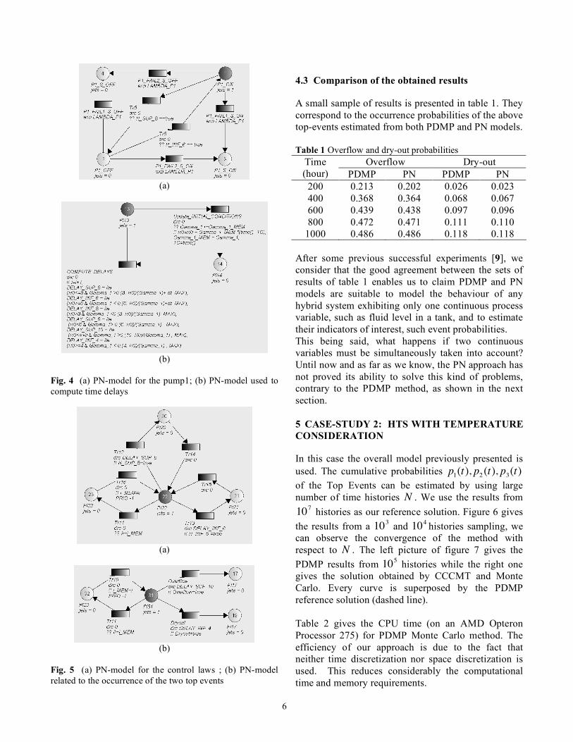
4 CASE-STUDY 1: HTS WITHOUT TEMPE-RATURE 4.1 The PDMP approach This approach is first applied. The general model presented in section 3 has been simplified for this case by canceling relations between temperature ! and both fluid level h and failure rates λc . Some numerical results thus obtained are gathered in table 1 of section 4.3. 4.2 The PN approach Petri nets are powerful tool for modeling in a concise way the behavior of any system. Because of the lack of space, the main features of this approach can not be described here, but they can be found in many papers already published (see, for instance, ref [7, 8]). However some information is given hereafter to explain how the PN-model can describe the dynamic evolution of the studied system. Some PN-models dedicated to our problem are presented in figures 4 and 5. In fact, we need seven PNs to model the HTS problem. Only four PNs are depicted. The one presented in figure 4a models the behaviour of pump1 (P1) and the PN located in figure 4b is used to update the initial conditions and to compute the different time delays to reach the specific levels defined in section 3.1. The PN presented in figure 5a is related to the control laws, and the other one in figure 5b indicates the possible occurrence of each considered top events, i.e., the overflow and the dryout.

6

(a)

(b)

Fig. 4 (a) PN-model for the pump1; (b) PN-model used to compute time delays

(a)

(b)

Fig. 5 (a) PN-model for the control laws ; (b) PN-model related to the occurrence of the two top events

4.3 Comparison of the obtained results A small sample of results is presented in table 1. They correspond to the occurrence probabilities of the above top-events estimated from both PDMP and PN models. Table 1 Overflow and dry-out probabilities

Overflow Dry-out Time (hour) PDMP PN PDMP PN

200 0.213 0.202 0.026 0.023 400 0.368 0.364 0.068 0.067 600 0.439 0.438 0.097 0.096 800 0.472 0.471 0.111 0.110

1000 0.486 0.486 0.118 0.118 After some previous successful experiments [9], we consider that the good agreement between the sets of results of table 1 enables us to claim PDMP and PN models are suitable to model the behaviour of any hybrid system exhibiting only one continuous process variable, such as fluid level in a tank, and to estimate their indicators of interest, such event probabilities. This being said, what happens if two continuous variables must be simultaneously taken into account? Until now and as far as we know, the PN approach has not proved its ability to solve this kind of problems, contrary to the PDMP method, as shown in the next section. 5 CASE-STUDY 2: HTS WITH TEMPERATURE CONSIDERATION In this case the overall model previously presented is used. The cumulative probabilities p

1(t), p

2(t), p

3(t)

of the Top Events can be estimated by using large number of time histories N . We use the results from 10

7 histories as our reference solution. Figure 6 gives the results from a 103 and 104 histories sampling, we can observe the convergence of the method with respect to N . The left picture of figure 7 gives the PDMP results from 105 histories while the right one gives the solution obtained by CCCMT and Monte Carlo. Every curve is superposed by the PDMP reference solution (dashed line). Table 2 gives the CPU time (on an AMD Opteron Processor 275) for PDMP Monte Carlo method. The efficiency of our approach is due to the fact that neither time discretization nor space discretization is used. This reduces considerably the computational time and memory requirements.

7

Fig. 6 PDMP results for N=10e3 and N=10e4 compared with reference solution

Fig. 7 PDMP results for N=10e5 and comparison of reference solution with CCMT solution

Table 2 CPU Time

Number of Histories N

CPU time 2.2 GHz

Estimation of relative error p

1(!)

103 0.98s 1.75%

104 10.03s 1.5%

105 1m37s 0.9%

106 16m37s 0.13%

6 CONCLUSIONS

Through a simple but not trivial test-case, it seems to us that the PDMP approach is an alternative way to correctly model the behaviour of hybrid systems and to evaluate their performance in terms of reliability and availability. Our next challenge is twofold. It consists in performing RAMS analyses of realistic size systems by means of the presented PDMP method and by using an extended PN model able to handle such

problems.

REFERENCES

1 Cocozza-Thivent, C. Processus stochastiques et Fiabilité des systèmes, Springer, 1997

2 Davis, M. Markov models and optimization. London: Chapman and Hall, 1993

3 Dufour, F. and Dutuit, Y. Dynamic reliability : A new model. In Proceedings of ESREL 2002 Lambda-Mu 13 Conference, 2002

4 Marseguerra, M. and Zio, E. The cell-to-boundary method in Monte Carlo based dynamic PSA. Reliability Engng System Safety, 1995, 45, 199-204.

5 Marseguerra, M. and Zio, E. Monte Carlo approach to PSA for dynamic process systems. Reliability Engng System Safety, 1996, 52, 227-241.

6 Tombuyses, B. and Aldemir, T. Continuous cell-to-cell mapping and dynamic PSA. In Proceedings of ICONE 4 conference, 1996.

7 Dutuit, Y., Châtelet, E., Signoret, J. P. and Thomas, P., Dependability modeling and evaluation by using stochastic Petri nets:

8

application to two test cases. Reliability Engng and System Safety, 1997, 55, 117-124.

8 Malhotra, A. and Trivedi, K. S., Dependapility modeling using Petri nets. IEEE Trans. Reliab., 1995, 44, 428-440.

9 Zhang, H., Dufour, F., Innal, F. and Dutuit, Y. Dynamic reliability and piecewise-deterministic processes. In Proceedings of Lambda-Mu 15 Conference, 2006

9