MODELING AND CIRCUIT-BASED

SIMULATION OF PHOTOVOLTAIC ARRAYS

Marcelo Gradella Villalva, Jonas Rafael Gazoli, Ernesto Ruppert Filho

University of Campinas (UNICAMP), Brazil

mvillalva@gmail.com, gazoli@gmail.com, ruppert@fee.unicamp.br

Abstract - This paper presents an easy and accurate

method of modeling photovoltaic arrays. The method is

used to obtain the parameters of the array model using

information from the datasheet. The photovoltaic array

model can be simulated with any circuit simulator. The

equations of the model are presented in details and the

model is validated with experimental data. Finally, sim-

ulation examples are presented. This paper is useful for

power electronics designers and researchers who need an

effective and straightforward way to model and simulate

photovoltaic arrays.

Keywords – PV array, modeling, simulation.

I. INTRODUCTION

A photovoltaic system converts sunlight into electricity.

The basic device of a photovoltaic system is the photovoltaic

cell. Cells may be grouped to form panels or modules. Panels

can be grouped to form large photovoltaic arrays. The term ar-

ray is usually employed to describe a photovoltaic panel (with

several cells connected in series and/or parallel) or a group

of panels. Most of time one are interested in modeling pho-

tovoltaic panels, which are the commercial photovoltaic de-

vices. This paper focuses on modeling photovoltaic modules

or panels composed of several basic cells. The term array used

henceforth means any photovoltaic device composed of sev-

eral basic cells. In the Appendix at the end of this paper there

are some explanations about how to model and simulate large

photovoltaic arrays composed of several panels connected in

series or in parallel.

The electricity available at the terminals of a photovoltaic

array may directly feed small loads such as lighting systems

and DC motors. Some applications require electronic con-

verters to process the electricity from the photovoltaic device.

These converters may be used to regulate the voltage and cur-

rent at the load, to control the power flow in grid-connected

systems and mainly to track the maximum power point (MPP)

of the device.

Photovoltaic arrays present a nonlinear I-V characteristic

with several parameters that need to be adjusted from experi-

mental data of practical devices. The mathematical model of

the photovoltaic array may be useful in the study of the dy-

namic analysis of converters, in the study of maximum power

point tracking (MPPT) algorithms and mainly to simulate the

photovoltaic system and its components using simulators.

This text presents in details the equations that form the the

I-V model and the method used to obtain the parameters of

the equation. The aim of this paper is to provide the reader

with all necessary information to develop photovoltaic array

models and circuits that can be used in the simulation of power

converters for photovoltaic applications.

II. MODELING OF PHOTOVOLTAIC ARRAYS

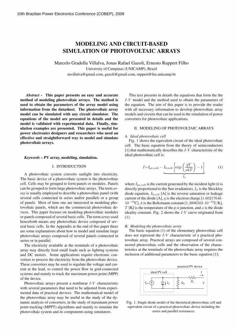
A. Ideal photovoltaic cellFig. 1 shows the equivalent circuit of the ideal photovoltaic

cell. The basic equation from the theory of semiconductors

[1] that mathematically describes the I-V characteristic of the

ideal photovoltaic cell is:

I=Ipv,cell − I0,cell

[

exp

(qV

akT

)

− 1

]

︸ ︷︷ ︸

Id

(1)

where Ipv,cell is the current generated by the incident light (it is

directly proportional to the Sun irradiation), Id is the Shockley

diode equation, I0,cell [A] is the reverse saturation or leakage

current of the diode [A], q is the electron charge [1.60217646 ·10−19C], k is the Boltzmann constant [1.3806503·10−23J/K],

T [K] is the temperature of the p-n junction, and a is the diode

ideality constant. Fig. 2 shows the I-V curve originated from

(1).

B. Modeling the photovoltaic arrayThe basic equation (1) of the elementary photovoltaic cell

does not represent the I-V characteristic of a practical pho-

tovoltaic array. Practical arrays are composed of several con-

nected photovoltaic cells and the observation of the charac-

teristics at the terminals of the photovoltaic array requires the

inclusion of additional parameters to the basic equation [1]:

I

VIpv IdRsRp

ideal PV cell

practical PV device

Fig. 1. Single-diode model of the theoretical photovoltaic cell and

equivalent circuit of a practical photovoltaic device including the

series and parallel resistances.

10th Brazilian Power Electronics Conference (COBEP), 2009

- =

I

V V V

Ipv Id

Fig. 2. Characteristic I-V curve of the photovoltaic cell. The net

cell current I is composed of the light-generated current Ipv and the

diode current Id.

I

V

(0, Isc)

(Voc, 0)

(Vmp, Imp)

current

source

source

voltage

MPP

Fig. 3. Characteristic I-V curve of a practical photovoltaic device

and the three remarkable points: short circuit (0, Isc), maximum

power point (Vmp, Imp) and open-circuit (Voc, 0).

I = Ipv − I0

[

exp

(V + RsI

Vta

)

− 1

]

−V + RsI

Rp

(2)

where Ipv and I0 are the photovoltaic and saturation currents

of the array and Vt = NskT/q is the thermal voltage of the

array with Ns cells connected in series. Cells connected in

parallel increase the current and cells connected in series pro-

vide greater output voltages. If the array is composed of Np

parallel connections of cells the photovoltaic and saturation

currents may be expressed as: Ipv=Ipv,cellNp, I0=I0,cellNp.

In (2) Rs is the equivalent series resistance of the array and Rp

is the equivalent parallel resistance. This equation originates

the I-V curve seen in Fig. 3, where three remarkable points

are highlighted: short circuit (0, Isc), maximum power point

(Vmp, Imp) and open-circuit (Voc, 0).Eq. (2) describes the single-diode model presented in Fig.

1. Some authors have proposed more sophisticated models

that present better accuracy and serve for different purposes.

For example, in [2–6] an extra diode is used to represent the

effect of the recombination of carriers. In [7] a three-diode

model is proposed to include the influence of effects which

are not considered by the previous models. For simplicity the

single-diode model of Fig. 1 is studied in this paper. This

model offers a good compromise between simplicity and ac-

curacy [8] and has been used by several authors in previous

works, sometimes with simplifications but always with the

basic structure composed of a current source and a parallel

diode [9–23]. The simplicity of the single-diode model with

the method for adjusting the parameters and the improvements

proposed in this paper make this model perfect for power elec-

tronics designers who are looking for an easy and effective

model for the simulation of photovoltaic devices with power

converters.

Manufacturers of photovoltaic arrays, instead of the I-V

equation, provide only a few experimental data about electri-

cal and thermal characteristics. Unfortunately some of the pa-

rameters required for adjusting photovoltaic array models can-

not be found in the manufacturers’s data sheets, such as the

light-generated or photovoltaic current, the series and shunt

resistances, the diode ideality constant, the diode reverse sat-

uration current, and the bandgap energy of the semiconductor.

All photovoltaic array datasheets bring basically the following

information: the nominal open-circuit voltage Voc,n, the nom-

inal short-circuit current Isc,n, the voltage at the maximum

power point Vmp, the current at the maximum power point

Imp, the open-circuit voltage/temperature coefficient KV , the

short-circuit current/temperature coefficient KI , and the max-

imum experimental peak output power Pmax,e. This informa-

tion is always provided with reference to the nominal or stan-

dard test conditions (STC) of temperature and solar irradia-

tion. Some manufacturers provide I-V curves for several irra-

diation and temperature conditions. These curves make easier

the adjustment and the validation of the desired mathematical

I-V equation. Basically this is all the information one can get

from datasheets of photovoltaic arrays.

Electric generators are generally classified as current or

voltage sources. The practical photovoltaic device presents an

hybrid behavior, which may be of current or voltage source de-

pending on the operating point, as shown in Fig. 3. The practi-

cal photovoltaic device has a series resistance Rs whose influ-

ence is stronger when the device operates in the voltage source

region, and a parallel resistance Rp with stronger influence in

the current source region of operation. The Rs resistance is

the sum of several structural resistances of the device [24].

The Rp resistance exists mainly due to the leakage current of

the p-n junction and depends on the fabrication method of the

photovoltaic cell. The value of Rp is generally high and some

authors [11–14, 17, 18, 25–28] neglect this resistance to sim-

plify the model. The value of Rs is very low and sometimes

this parameter is neglected too [26, 29–31].

The I-V characteristic of the photovoltaic device shown in

Fig. 3 depends on the internal characteristics of the device

(Rs, Rp) and on external influences such as irradiation level

and temperature. The amount of incident light directly affects

the generation of charge carriers and consequently the current

generated by the device. The light-generated current (Ipv) of

the elementary cells, without the influence of the series and

parallel resistances, is difficult to determine. Datasheets only

inform the nominal short-circuit current (Isc,n), which is the

maximum current available at the terminals of the practical

device. The assumption Isc ≈ Ipv is generally used in photo-

voltaic models because in practical devices the series resis-

tance is low and the parallel resistance is high. The light-

generated current of the photovoltaic cell depends linearly on

the solar irradiation and is also influenced by the temperature

according to the following equation [19, 32–34]:

Ipv = (Ipv,n + KI∆T)G

Gn

(3)

where Ipv,n [A] is the light-generated current at the nominal

condition (usually 25 C and 1000W/m2), ∆T = T − Tn

(being T and Tn the actual and nominal temperatures [K]), G

[W/m2] is the irradiation on the device surface, and Gn is the

nominal irradiation.

The diode saturation current I0 and its dependence on the

temperature may be expressed by (4) [32, 33, 35–38]:

I0 = I0,n

(Tn

T

)3exp

[qEg

ak

(1

Tn

−1

T

)]

(4)

where Eg is the bandgap energy of the semiconductor (Eg ≈1.12 eV for the polycrystalline Si at 25 C [11, 32]), and I0,n

is the nominal saturation current:

I0,n =Isc,n

exp

(Voc,n

aVt,n

)

− 1

(5)

with Vt,n being the thermal voltage of Ns series-connected

cells at the nominal temperature Tn.

The saturation current I0 of the photovoltaic cells that com-

pose the device depend on the saturation current density of the

semiconductor (J0, generally given in [A/cm2]) and on the ef-

fective area of the cells. The current density J0 depends on the

intrinsic characteristics of the photovoltaic cell, which depend

on several physical parameters such as the coefficient of diffu-

sion of electrons in the semiconductor, the lifetime of minority

carriers, the intrinsic carrier density, and others [7]. This kind

of information is not usually available for commercial photo-

voltaic arrays. In this paper the nominal saturation current I0,n

is indirectly obtained from the experimental data through (5),

which is obtained by evaluating (2) at the nominal open-circuit

condition, with V = Voc,n, I = 0, and Ipv ≈ Isc,n.

The value of the diode constant a may be arbitrarily chosen.

Many authors discuss ways to estimate the correct value of this

constant [8, 11]. Usually 1 ≤ a ≤ 1.5 and the choice depends

on other parameters of the I-V model. Some values for aare found in [32] based on empirical analysis. As [8] says,

there are different opinions about the best way to choose a.

Because a expresses the degree of ideality of the diode and it is

totally empirical, any initial value of a can be chosen in order

to adjust the model. The value of a can be later modified in

order to improve the model fitting if necessary. This constant

affects the curvature of the I-V characteristic and varying acan slightly improve the model accuracy.

C. Improving the modelThe photovoltaic model described in the previous section

can be improved if equation (4) is replaced by:

I0 =Isc,n + KI∆T

exp

(Voc,n + KV∆T

aVt

)

− 1

(6)

This modification aims to match the open-circuit voltages

of the model with the experimental data for a very large range

of temperatures. Eq. (6) is obtained from (5) by including

in the equation the current and voltage coefficients KV and

KI. The saturation current I0 is strongly dependent on the

temperature and (6) proposes a different approach to express

the dependence of I0 on the temperature so that the net effect

of the temperature is the linear variation of the open-circuit

voltage according the the practical voltage/temperature coef-

ficient. This equation simplifies the model and cancels the

model error at the vicinities of the open-circuit voltages and

consequently at other regions of the I-V curve.

The validity of the model with this new equation has been

tested through computer simulation and through comparison

with experimental data. One interesting fact about the correc-

tion introduced with (6) is that the coefficient KV from the

manufacturer’s datasheet appears in the equation. The volt-

age/temperature coefficient KV brings important information

necessary to achieve the best possible I-V curve fitting for

temperatures different of the nominal value.

If one wish to keep the traditional equation (4) [32, 33, 35–

38], instead of using (6), it is possible to obtain the best value

of Eg for the model so that the open-circuit voltages of the

model are matched with the open-circuit voltages of the real

array in the range Tn < T < Tmax. By equaling (4) and (6)

and solving for Eg at T = Tmax one gets:

Eg = − ln

(Isc,Tmax

I0,n

) (Tn

Tmax

)3

exp

(qVoc,Tmax

aNskTmax

)

− 1

·

· akTnTmax

q (Tn − Tmax)

(7)

where Isc,Tmax = Isc,n + KI∆T and Voc,Tmax = Voc,n +KV∆T, with ∆T = Tmax − Tn.

D. Adjusting the model

Two parameters remain unknown in (2), which are Rs and

Rp. A few authors have proposed ways to mathematically de-

termine these resistances. Although it may be useful to have

a mathematical formula to determine these unknown parame-

ters, any expression for Rs and Rp will always rely on exper-

imental data. Some authors propose varying Rs in an iterative

process, incrementing Rs until the I-V curve visually fits the

experimental data and then vary Rp in the same fashion. This

is a quite poor and inaccurate fitting method, mainly because

Rs and Rp may not be adjusted separately if a good I-V model

is desired.

This paper proposes a method for adjusting Rs and Rp

based on the fact that there is an only pair Rs,Rp that war-

ranties that Pmax,m = Pmax,e = VmpImp at the (Vmp, Imp)point of the I-V curve, i.e. the maximum power calculated

by the I-V model of (2), Pmax,m, is equal to the maximum ex-

perimental power from the datasheet, Pmax,e , at the maximum

power point (MPP). Conventional modeling methods found in

the literature take care of the I-V curve but forget that the

P -V (power vs. voltage) curve must match the experimental

data too. Works like [26, 39] gave attention to the necessity

of matching the power curve but with different or simplified

models. In [26], for example, the series resistance of the array

model is neglected.

The relation between Rs and Rp, the only unknowns of (2),

may be found by making Pmax,m = Pmax,e and solving the

resulting equation for Rs, as (8) and (9) show.

0 5 10 15 20 25 30 350

20

40

60

80

100

120

140

160

180

200

V: 26.3

P: 200.1

V [V]

MPP

Rs increasing

P[W

]

Fig. 4. P -V curves plotted for different values of Rs and Rp.

Pmax,m =

= Vmp

Ipv − I0

[

exp

(q

kT

Vmp + RsImp

aNs

)

− 1

]

−Vmp + RsImp

Rp

= Pmax,e

− (8)

Rp = Vmp(Vmp + ImpRs)/

VmpIpv − VmpI0 exp

[(Vmp + ImpRs)

Nsa

q

kT

]

+VmpI0 − Pmax,e

+ (9)

Eq. (9) means that for any value of Rs there will be a value

of Rp that makes the mathematical I-V curve cross the exper-

imental (Vmp, Imp) point.

E. Iterative solution of Rs and Rp

The goal is to find the value of Rs (and hence Rp) that

makes the peak of the mathematical P -V curve coincide with

the experimental peak power at the (Vmp, Imp) point. This

requires several iterations until Pmax,m = Pmax,e.

In the iterative process Rs must be slowly incremented start-

ing from Rs = 0. Adjusting the P -V curve to match the ex-

perimental data requires finding the curve for several values

of Rs and Rp. Actually plotting the curve is not necessary, as

only the peak power value is required. Figs. 4 and 6 illustrate

how this iterative process works. In Fig. 4 as Rs increases

the P -V curve moves to the left and the peak power (Pmax,m)

goes towards the experimental MPP. Fig. 5 shows the con-

tour drawn by the peaks of the power curves for several val-

ues of Rs (this example uses the parameters of the Kyocera

KC200GT solar array [40]). For every P -V curve of Fig. 4

there is a corresponding I-V curve in Fig. 6. As expected

from (9), all I-V curves cross the desired experimental MPP

point at (Vmp, Imp).Plotting the P -V and I-V curves requires solving (2) for

I ∈ [0, Isc,n] and V ∈ [0, Voc,n]. Eq. (2) does not have a

direct solution because I = f(V, I) and V = f(I, V ). This

transcendental equation must be solved by a numerical method

and this imposes no difficulty. The I-V points are easily ob-

tained by numerically solving g(V, I) = I − f(V, I) = 0 for a

set of V values and obtaining the corresponding set of I points.

Obtaining the P -V points is straightforward.

0 5 10 15 20 25 30 350

50

100

150

200

250

V: 26.3

P: 200.1

V [V]

Pm

ax

[W]

Fig. 5. Pmax,m vs. V for several values of Rs > 0.

0 5 10 15 20 25 30 350

1

2

3

4

5

6

7

8V: 26.3

I: 7.61

V [V]

MPP

I[A

]

Fig. 6. I-V curves plotted for different values of Rs and Rp.

The iterative method gives the solution Rs = 0.221 Ω for

the KC200GT array. Fig. 5 shows a plot of Pmax,m as a func-

tion of V for several values of Rs. There is an only point, cor-

responding to a single value of Rs, that satisfies the imposed

condition Pmax,m = VmpImp at the (Vmp, Imp) point. Fig. 7

shows a plot of Pmax,m as a function of Rs for I = Imp and

V = Vmp. This plot shows that Rs = 0.221 Ω is the desired

solution, in accordance with the result of the iterative method.

This plot may be an alternative way for graphically finding the

solution for Rs.

0 0.1 0.2 0.3 0.4 0.5 0.6 0.7200

202

204

206

208

210

212

214

216

218

220

R: 0.221

P: 200.1

Rs [Ω]

Pm

ax

[W]

Fig. 7. Pmax = f(Rs) with I = Imp and V = Vmp.

0 5 10 15 20 25 30 350

1

2

3

4

5

6

7

8V: 0

I: 8.21

V: 26.3

I: 7.61

V: 32.9

I: 0

I[A

]

V [V]

Fig. 8. I-V curve adjusted to three remarkable points.

0 5 10 15 20 25 30 350

20

40

60

80

100

120

140

160

180

200

V: 0

P: 0

V: 26.3

P: 200.1

V: 32.9

P: 0

P[W

]

V [V]

Fig. 9. P -V curve adjusted to three remarkable points.

Figs. 8 and 9 show the I-V and P -V curves of the

KC200GT photovoltaic array adjusted with the proposed

method. The model curves exactly match with the experi-

mental data at the three remarkable points provided by the

datasheet: short circuit, maximum power, and open circuit.

Table I shows the experimental parameters of the array ob-

tained from the datasheeet and Table II shows the adjusted pa-

rameters and model constants.

F. Further improving the modelThe model developed in the preceding sections may be fur-

ther improved by taking advantage of the iterative solution of

Rs and Rp. Each iteration updates Rs and Rp towards the

TABLE I

Parameters of the KC200GT PV array at

25C, AM1.5, 1000 W/m2.

Imp 7.61 AVmp 26.3 VPmax,e 200.143 WIsc 8.21 AVoc 32.9 VKV −0.1230 V/KKI 0.0032 A/KNs 54

TABLE II

Parameters of the adjusted model of the KC200GT

solar array at nominal operating conditions.

Imp 7.61 AVmp 26.3 VPmax,m 200.143 WIsc 8.21 AVoc 32.9 VI0,n 9.825 · 10−8 A

Ipv 8.214 Aa 1.3Rp 415.405 ΩRs 0.221 Ω

best model solution, so equation (10) may be introduced in the

model.

Ipv,n =Rp + Rs

Rp

Isc,n (10)

Eq. (10) uses the resistances Rs and Rp to determine Ipv 6=Isc. The values of Rs and Rp are initially unknown but as the

solution of the algorithm is refined along successive iterations

the values of Rs and Rp tend to the best solution and (10)

becomes valid and effectively determines the light-generated

current Ipv taking in account the influence of the series and

parallel resistances of the array. Initial guesses for Rs and Rp

are necessary before the iterative process starts. The initial

value of Rs may be zero. The initial value of Rp may be given

by:

Rp,min =Vmp

Isc,n − Imp

−Voc,n − Vmp

Imp

(11)

Eq. (11) determines the minimum value of Rp, which is

the slope of the line segment between the short-circuit and the

maximum-power remarkable points. Although Rp is still un-

known, it surely is greater than Rp,min and this is a good initial

guess.

G. Modeling algorithmThe simplified flowchart of the iterative modeling algorithm

is illustrated in Fig. 10.

III. VALIDATING THE MODEL

As Tables I and II and Figs. 8 and 9 have shown, the de-

veloped model and the experimental data are exactly matched

at the nominal remarkable points of the I-V curve and the ex-

perimental and mathematical maximum peak powers coincide.

The objective of adjusting the mathematical I-V curve at the

three remarkable points was successfully achieved.

In order to test the validity of the model a comparison with

other experimental data (different of the nominal remarkable

points) is very useful. Fig. 11 shows the mathematical I-Vcurves of the KC200GT solar panel plotted with the exper-

imental data at three different temperature conditions. Fig.

12 shows the I-V curves at different irradiations. The circu-

lar markers in the graphs represent experimental (V, I) points

Inputs: T , GI0 , eq. (4) or (6)

Rs = 0Rp = Rp,min, eq. (11)

εPmax > tol

Ipv,n , eq. (10)

Ipv and Isc, eq. (3)

Rp, eq. (9)

Solve eq. (2) for 0 ≤ V ≤ Voc,n

Calculate P for 0 ≤ V ≤ Voc,n

Find Pmax

εPmax = ‖Pmax − Pmax,e‖Increment Rs

yes

noEND

Fig. 10. Algorithm of the method used to adjust the I-V model.

0 5 10 15 20 25 300

1

2

3

4

5

6

7

8

9

KYOCERA KC200GT - 1000 W/m2

25 °C50 °C75 °C

I[A

]

V [V]

Fig. 11. I-V model curves and experimental data of the KC200GT

solar array at different temperatures, 1000 W/m2.

extracted from the datasheet. Some points are not exactly

matched because the model is not perfect, although it is ex-

act at the remarkable points and sufficiently accurate for other

points. The model accuracy may be slightly improved by run-

ning more iterations with other values of the constant a, with-

out modifications in the algorithm.

Fig. 13 shows the mathematical I-V curves of the Solarex

MSX60 solar panel [41] plotted with the experimental data

at two different temperature conditions. Fig. 14 shows the

P -V curves obtained at the two temperatures. The circular

markers in the graphs represent experimental (V, I) and (V, P )points extracted from the datasheet. Fig. 14 proves that the

model accurately matches with the experimental data both in

the current and power curves, as expected.

IV. SIMULATION OF THE PHOTOVOLTAIC ARRAY

The photovoltaic array can be simulated with an equivalent

circuit model based on the photovoltaic model of Fig. 1. Two

simulation strategies are possible.

Fig. 15 shows a circuit model using one current source

0 5 10 15 20 25 300

1

2

3

4

5

6

7

8

9

KYOCERA KC200GT - 25 °C

1000 W/m2

800 W/m2

600 W/m2

400 W/m2

I[A

]

V [V]

Fig. 12. I-V model curves and experimental data of the KC200GT

solar array at different irradiations, 25 C.

0 5 10 15 200

0.5

1

1.5

2

2.5

3

3.5

4

4.5

SOLAREX MSX60 - 1000 W/m2

25 °C

75 °C

I[A

]

V [V]

Fig. 13. I-V model curves and experimental data of the MSX60

solar array at different temperatures, 1000 W/m2.

0 5 10 15 200

10

20

30

40

50

60

SOLAREX MSX60 - 1000 W/m2

25 °C

75 °C

P[W

]

V [V]

Fig. 14. P -V model curves and experimental data of the MSX60

solar array at different temperatures, 1000 W/m2.

+-

+ -

Ipv − I0

[

exp

(V + RsI

Vta

)

− 1

]

V

V

I

I

I0

Im

Ipv

Rp

Rs

Fig. 15. Photovoltaic array model circuit with a controlled current

source, equivalent resistors and the equation of the model current

(Im).

(Im) and two resistors (Rs and Rp). This circuit can be im-

plemented with any circuit simulator. The value of the model

current Im is calculated by the computational block that has

V , I , I0 and Ipv as inputs. I0 is obtained from (4) or (6) and

Ivp is obtained from (3). This computational block may be

implemented with any circuit simulator able to evaluate math

functions.

Fig. 16 shows another circuit model composed of only one

current source. The value of the current is obtained by numer-

ically solving the I-V equation. For every value of V a corre-

sponding I that satisfies the I-V equation (2) is obtained. The

solution of (2) can be implemented with a numerical method

in any circuit simulator that accepts embedded programming.

This is the simulation strategy proposed in [42].

Other authors have proposed circuits for simulating photo-

voltaic arrays that are based on simplified equations and/or

require lots of computational effort [12, 26, 27, 43]. In [12]

a circuit-based photovoltaic model is composed of a current

source driven by an intricate and inaccurate equation where

the parallel resistance is neglected. In [26] an intricate PSpice-

based simulation was presented, where the I-V equation is

numerically solved within the PSpice software. Although in-

teresting, the approach found in [26] is excessively elaborated

and concerns the simplified photovoltaic model without the

series resistance. In [27] a simple circuit-based photovoltaic

model is proposed where the parallel resistance is neglected.

In [43] a circuit-based model was proposed based on the piece-

wise approximation of the I-V curve. Although interesting

and relatively simple, this method [43] does not provide a so-

lution to find the parameters of the I-V equation and the circuit

model requires many components.

Figs. 17 and 18 show the photovoltaic model circuits im-

plemented with MATLAB/SIMULINK (using the SymPow-

erSystems blockset) and PSIM using the simulation strategy

of Fig. 15. Both circuit models work perfectly and may be

used in the simulation of power electronics converters for pho-

tovoltaic systems. Figs. 19 and 20 show the I-V curves of

the Solarex MSX60 solar panel [41] simulated with the MAT-

LAB/SIMULINK and PSIM circuits.

V. CONCLUSION

This paper has analyzed the development of a method for

the mathematical modeling of photovoltaic arrays. The objec-

tive of the method is to fit the mathematical I-V equation to

+-

Numerical solution of eq. (2)

V

V

I

I

Fig. 16. Photovoltaic array model circuit with a controlled current

source and a computational block that solves the I-V equation.

Fig. 17. Photovoltaic circuit model built with

MATLAB/SIMULINK.

the experimental remarkable points of the I-V curve of the

practical array. The method obtains the parameters of the I-

V equation by using the following nominal information from

the array datasheet: open-circuit voltage, short-circuit current,

maximum output power, voltage and current at the maximum

power point, current/temperature and voltage/temperature co-

efficients. This paper has proposed an effective and straight-

forward method to fit the mathematical I-V curve to the three

Fig. 18. Photovoltaic circuit model built with PSIM.

0 5 10 15 200

0.5

1

1.5

2

2.5

3

3.5

4

25°C,1000W/m2

25°C,800W/m2

75°C,1000W/m2

75°C,800W/m2

Fig. 19. I-V curves of the model simulated with

MATLAB/SIMULINK.

Fig. 20. I-V curves of the model simulated with PSIM.

(V, I) remarkable points without the need to guess or to esti-

mate any other parameters except the diode constant a. This

paper has proposed a closed solution for the problem of finding

the parameters of the single-diode model equation of a prac-

tical photovoltaic array. Other authors have tried to propose

single-diode models and methods for estimating the model pa-

rameters, but these methods always require visually fitting the

mathematical curve to the I-V points and/or graphically ex-

tracting the slope of the I-V curve at a given point and/or suc-

cessively solving and adjusting the model in a trial and error

process. Some authors have proposed indirect methods to ad-

just the I-V curve through artificial intelligence [15, 44–46]

and interpolation techniques [25]. Although interesting, such

methods are not very practical and are unnecessarily compli-

cated and require more computational effort than it would be

expected for this problem. Moreover, frequently in these mod-

els Rs and Rp are neglected or treated as independent parame-

ters, which is not true if one wish to correctly adjust the model

so that the maximum power of the model is equal to the maxi-

mum power of the practical array.

An equation to express the dependence of the diode satura-

tion current I0 on the temperature was proposed and used in

the model. The results obtained in the modeling of two prac-

tical photovoltaic arrays have demonstrated that the equation

is effective and permits to exactly adjust the I-V curve at the

open-circuit voltages at temperatures different of the nominal.

Moreover, the assumption Ipv ≈ Isc used in most of pre-

vious works on photovoltaic modeling was replaced in this

method by a relation between Ipv and Isc based on the series

and parallel resistances. The proposed iterative method for

solving the unknown parameters of the I-V equation allows to

determine the value of Ipv, which is different of Isc.

This paper has presented in details the equations that con-

stitute the single-diode photovoltaic I-V model and the algo-

rithm necessary to obtain the parameters of the equation. In or-

der to show the practical use of the proposed modeling method

this paper has presented two circuit models that can be used to

simulate photovoltaic arrays with circuit simulators.

This paper provides the reader with all necessary informa-

tion to easily develop a single-diode photovoltaic array model

for analyzing and simulating a photovoltaic array. Programs

and ready-to-use circuit models are available for download at:

http://sites.google.com/site/mvillalva/pvmodel.

APPENDIX - ASSOCIATION OF PV ARRAYS

In the previous sections this paper has dealt with the model-

ing and simulation of photovoltaic arrays that are single panels

or modules composed of several interconnected basic photo-

voltaic cells. Large arrays composed of several panels may be

modeled in the same way, provided that the equivalent param-

eters (short-circuit current, open-circuit voltage) are properly

inserted in the modeling process. As a result, the equivalent

parameters (resistances, currents, etc) of the association are

obtained. Generally experimental data are available only for

commercial low-power modules and this is the reason why this

paper has chosen to deal with small arrays. The term array has

been used throughout this paper to mean small commercial

photovoltaic modules or panels. This appendix shows how to

I

I

I

V

V

V

(a)

(b)

(c)

Ipv Id

. . .

. . .

. . .

. . . ... ...

...

...

...

...

RsNser

RpNser

IpvNpar

IdNpar

Rs/Npar

Rp/Npar

IpvNpar IdNpar

RsNser/Npar

RpNser/Npar

Fig. 21. (a) Array of Nser modules connected in series, (b) Array of

Npar modules connected in parallel, and (c) array composed of Nser

x Npar modules.

model and simulate large arrays composed of several series or

parallel modules. Here, unlike in the rest of this paper, module

and array have distinct meanings.

Fig. 21a shows an array composed of several identic mod-

ules connected in series. The output voltage is increased pro-

portionately to Nser and the currents remain unchanged. The

equivalent series and parallel resistances are directly propor-

tional to the number of modules.

Fig. 21b shows an array composed of several identic mod-

ules connected in parallel. The association provides increased

output current and the output voltage is unchanged. The equiv-

alent series and parallel resistances are inversely proportional

to the number of parallel modules.

Fig. 21c shows a photovoltaic array composed of several

modules connected in series and parallel. In this case the

equivalent resistances depend on the number of series and par-

allel connections.

For any given array formed by Nser x Npar identic modules

the following equivalent I-V equation is valid:

I = IpvNpar − I0Npar

exp

V + Rs

(Nser

Npar

)

I

VtaNser

− 1

−

−

V + Rs

(Nser

Npar

)

I

Rp

(Nser

Npar

)

(12)

+-

+ -

I0

Im

IpvIpvNpar − I0Npar

exp

V + Rs

(Nser

Npar

)

I

VtaNser

− 1

V

V

I

I

RpNser/Npar

RsNser/Npar

Fig. 22. Model circuit of array composed of Nser x Npar modules.

where Ipv, I0, Rs, Rp, and Vt are parameters of individual

modules. Please notice that Ns (the number of elementary

series cells of the individual photovoltaic module) used in the

preceding sections is different of Nser.

The photovoltaic array can be simulated with the modified

I-V equation (12). The simulation circuit presented previ-

ously must be modified according to the number of associated

modules. The Nser and Npar indexes must be inserted in the

model, respecting equation (12), as shown in Fig. 22.

REFERENCES

[1] H. S. Rauschenbach. Solar cell array design handbook.

Van Nostrand Reinhold, 1980.

[2] J. A. Gow and C. D. Manning. Development of a photo-

voltaic array model for use in power-electronics simula-

tion studies. Electric Power Applications, IEE Proceed-

ings, 146(2):193–200, 1999.

[3] J. A. Gow and C. D. Manning. Development of a model

for photovoltaic arrays suitable for use in simulation stud-

ies of solar energy conversion systems. In Proc. 6th Inter-

national Conference on Power Electronics and Variable

Speed Drives, p. 69–74, 1996.

[4] N. Pongratananukul and T. Kasparis. Tool for automated

simulation of solar arrays using general-purpose simula-

tors. In Proc. IEEE Workshop on Computers in Power

Electronics, p. 10–14, 2004.

[5] S. Chowdhury, G. A. Taylor, S. P. Chowdhury, A. K.

Saha, and Y. H. Song. Modelling, simulation and per-

formance analysis of a PV array in an embedded envi-

ronment. In Proc. 42nd International Universities Power

Engineering Conference, UPEC, p. 781–785, 2007.

[6] J. Hyvarinen and J. Karila. New analysis method for

crystalline silicon cells. In Proc. 3rd World Conference

on Photovoltaic Energy Conversion, v. 2, p. 1521–1524,

2003.

[7] Kensuke Nishioka, Nobuhiro Sakitani, Yukiharu Uraoka,

and Takashi Fuyuki. Analysis of multicrystalline sil-

icon solar cells by modified 3-diode equivalent circuit

model taking leakage current through periphery into con-

sideration. Solar Energy Materials and Solar Cells,

91(13):1222–1227, 2007.

[8] C. Carrero, J. Amador, and S. Arnaltes. A single proce-

dure for helping PV designers to select silicon PV mod-

ule and evaluate the loss resistances. Renewable Energy,

2007.

[9] E. Koutroulis, K. Kalaitzakis, and V. Tzitzilonis. Devel-

opment of a FPGA-based system for real-time simula-

tion of photovoltaic modules. Microelectronics Journal,

2008.

[10] G. E. Ahmad, H. M. S. Hussein, and H. H. El-Ghetany.

Theoretical analysis and experimental verification of PV

modules. Renewable Energy, 28(8):1159–1168, 2003.

[11] Geoff Walker. Evaluating MPPT converter topologies us-

ing a matlab PV model. Journal of Electrical & Electron-

ics Engineering, Australia, 21(1), 2001.

[12] M. Veerachary. PSIM circuit-oriented simulator model

for the nonlinear photovoltaic sources. IEEE Transac-

tions on Aerospace and Electronic Systems, 42(2):735–

740, April 2006.

[13] Ali Naci Celik and NasIr Acikgoz. Modelling and ex-

perimental verification of the operating current of mono-

crystalline photovoltaic modules using four- and five-

parameter models. Applied Energy, 84(1):1–15, January

2007.

[14] Yeong-Chau Kuo, Tsorng-Juu Liang, and Jiann-Fuh

Chen. Novel maximum-power-point-tracking controller

for photovoltaic energy conversion system. IEEE Trans-

actions on Industrial Electronics, 48(3):594–601, June

2001.

[15] M. T. Elhagry, A. A. T. Elkousy, M. B. Saleh, T. F. Elshat-

ter, and E. M. Abou-Elzahab. Fuzzy modeling of photo-

voltaic panel equivalent circuit. In Proc. 40th Midwest

Symposium on Circuits and Systems, v. 1, p. 60–63, Au-

gust 1997.

[16] Shengyi Liu and R. A. Dougal. Dynamic multiphysics

model for solar array. IEEE Transactions on Energy Con-

version, 17(2):285–294, 2002.

[17] Weidong Xiao, W. G. Dunford, and A. Capel. A novel

modeling method for photovoltaic cells. In Proc. IEEE

35th Annual Power Electronics Specialists Conference,

PESC, v. 3, p. 1950–1956, 2004.

[18] Y. Yusof, S. H. Sayuti, M. Abdul Latif, and M. Z. C.

Wanik. Modeling and simulation of maximum power

point tracker for photovoltaic system. In Proc. National

Power and Energy Conference, PECon, p. 88–93, 2004.

[19] D. Sera, R. Teodorescu, and P. Rodriguez. PV panel

model based on datasheet values. In Proc. IEEE Inter-

national Symposium on Industrial Electronics, ISIE, p.

2392–2396, 2007.

[20] M. A. Vitorino, L. V. Hartmann, A. M. N. Lima, and

M. B. R. Correa. Using the model of the solar cell for

determining the maximum power point of photovoltaic

systems. In Proc. European Conference on Power Elec-

tronics and Applications, p. 1–10, 2007.

[21] D. Dondi, D. Brunelli, L. Benini, P. Pavan, A. Bertac-

chini, and L. Larcher. Photovoltaic cell modeling for so-

lar energy powered sensor networks. In Proc. 2nd Inter-

national Workshop on Advances in Sensors and Interface,

IWASI, p. 1–6, 2007.

[22] H. Patel and V. Agarwal. MATLAB-based modeling to

study the effects of partial shading on PV array char-

acteristics. IEEE Transactions on Energy Conversion,

23(1):302–310, 2008.

[23] Wang Yi-Bo, Wu Chun-Sheng, Liao Hua, and Xu Hong-

Hua. Steady-state model and power flow analysis of grid-

connected photovoltaic power system. In Proc. IEEE In-

ternational Conference on Industrial Technology, ICIT,

p. 1–6, 2008.

[24] France Lasnier and Tony Gan Ang. Photovoltaic engi-

neering handbook. Adam Hilger, 1990.

[25] K. Khouzam, C. Khoon Ly, C.and Koh, and Poo Yong

Ng. Simulation and real-time modelling of space photo-

voltaic systems. In IEEE 1st World Conference on Pho-

tovoltaic Energy Conversion, Conference Record of the

24th IEEE Photovoltaic Specialists Conference, v. 2, p.

2038–2041, 1994.

[26] M. C. Glass. Improved solar array power point model

with SPICE realization. In Proc. 31st Intersociety En-

ergy Conversion Engineering Conference, IECEC, v. 1,

p. 286–291, August 1996.

[27] I. H. Altas and A. M. Sharaf. A photovoltaic array

simulation model for matlab-simulink GUI environment.

In Proc. International Conference on Clean Electrical

Power ,ICCEP, p. 341–345, 2007.

[28] E. Matagne, R. Chenni, and R. El Bachtiri. A photo-

voltaic cell model based on nominal data only. In Proc.

International Conference on Power Engineering, Energy

and Electrical Drives, POWERENG, p. 562–565, 2007.

[29] Yun Tiam Tan, D. S. Kirschen, and N. Jenkins. A

model of PV generation suitable for stability analysis.

IEEE Transactions on Energy Conversion, 19(4):748–

755, 2004.

[30] A. Kajihara and A. T. Harakawa. Model of photovoltaic

cell circuits under partial shading. In Proc. IEEE Inter-

national Conference on Industrial Technology, ICIT, p.

866–870, 2005.

[31] N. D. Benavides and P. L. Chapman. Modeling the ef-

fect of voltage ripple on the power output of photovoltaic

modules. IEEE Transactions on Industrial Electronics,

55(7):2638–2643, 2008.

[32] W. De Soto, S. A. Klein, and W. A. Beckman. Improve-

ment and validation of a model for photovoltaic array per-

formance. Solar Energy, 80(1):78–88, January 2006.

[33] Q. Kou, S. A. Klein, and W. A. Beckman. A method for

estimating the long-term performance of direct-coupled

PV pumping systems. Solar Energy, 64(1-3):33–40,

September 1998.

[34] A. Driesse, S. Harrison, and P. Jain. Evaluating the ef-

fectiveness of maximum power point tracking methods

in photovoltaic power systems using array performance

models. In Proc. IEEE Power Electronics Specialists

Conference, PESC, p. 145–151, 2007.

[35] R. A. Messenger and J. Ventre. Photovoltaic systems en-

gineering. CRC Press, 2004.

[36] F. Nakanishi, T. Ikegami, K. Ebihara, S. Kuriyama, and

Y. Shiota. Modeling and operation of a 10 kW photo-

voltaic power generator using equivalent electric circuit

method. In Conference Record of the 28th IEEE Photo-

voltaic Specialists Conference, p. 1703–1706, September

2000.

[37] J. Crispim, M. Carreira, and R. Castro. Validation of

photovoltaic electrical models against manufacturers data

and experimental results. In Proc. International Con-

ference on Power Engineering, Energy and Electrical

Drives, POWERENG, p. 556–561, 2007.

[38] K.H. Hussein, I. Muta, T. Hoshino, and M. Osakada.

Maximum photovoltaic power tracking: an algorithm for

rapidly changing atmospheric conditions. In Generation,

Transmission and Distribution, IEE Proceedings-, v. 142,

p. 59–64, January 1995.

[39] E. I. Ortiz-Rivera and F. Z. Peng. Analytical model for

a photovoltaic module using the electrical characteristics

provided by the manufacturer data sheet. In Proc. IEEE

36th Power Electronics Specialists Conference, PESC, p.

2087–2091, 2005.

[40] KC200GT high efficiency multicrystal photovoltaic mod-

ule datasheet.

[41] Solarex MSX60 and MSX64 solar arrays datasheet,

1998.

[42] M. M. Casaro and D. C. Martins. Modelo de arranjo fo-

tovoltaico destinado a analises em eletronica de potencia.

Revista Eletronica de Potencia, Sociedade Brasileira

de Eletronica de Potencia (SOBRAEP), 13(3):141–146,

2008.

[43] R. C. Campbell. A circuit-based photovoltaic array model

for power system studies. In Proc. 39th North American

Power Symposium, NAPS, p. 97–101, 2007.

[44] Th. F. Elshatter, M. T. Elhagry, E. M. Abou-Elzahab,

and A. A. T. Elkousy. Fuzzy modeling of photovoltaic

panel equivalent circuit. In Conference Record of the

28th IEEE Photovoltaic Specialists Conference, p. 1656–

1659, 2000.

[45] M. Balzani and A. Reatti. Neural network based model of

a PV array for the optimum performance of PV system. In

Proc. PhD Research in Microelectronics and Electronics,

v. 2, p. 123–126, 2005.

[46] H. Mekki, A. Mellit, H. Salhi, and B. Khaled. Model-

ing and simulation of photovoltaic panel based on artifi-

cial neural networks and VHDL-language. In Proc. 14th

IEEE International Conference on Electronics, Circuits

and Systems, ICECS, p. 58–61, 2007.