Seediscussions,stats,andauthorprofilesforthispublicationat:https://www.researchgate.net/publication/51668658

Physiologicalnoisereductionusingvolumetricfunctionalmagneticresonanceinverseimaging

ArticleinHumanBrainMapping·December2012

DOI:10.1002/hbm.21403·Source:PubMed

CITATIONS

13

READS

32

7authors,including:

Fa-HsuanLin

NationalTaiwanUniversity

126PUBLICATIONS2,426CITATIONS

SEEPROFILE

ThomasWitzel

HarvardUniversity

91PUBLICATIONS1,930CITATIONS

SEEPROFILE

ThomasZeffiro

MassachusettsGeneralHospital

144PUBLICATIONS7,765CITATIONS

SEEPROFILE

Fu-NienWang

NationalTsingHuaUniversity

27PUBLICATIONS296CITATIONS

SEEPROFILE

Allin-textreferencesunderlinedinbluearelinkedtopublicationsonResearchGate,

lettingyouaccessandreadthemimmediately.

Availablefrom:ThomasZeffiro

Retrievedon:15September2016

r Human Brain Mapping 0000:00–00 (2011) r

Physiological Noise Reduction Using VolumetricFunctional Magnetic Resonance Inverse Imaging

Fa-Hsuan Lin,1,2 Aapo Nummenmaa,2,3 Thomas Witzel,4

Jonathan R. Polimeni,2 Thomas A. Zeffiro,5 Fu-Nien Wang,6*and John W. Belliveau2

1Institute of Biomedical Engineering, National Taiwan University, Taipei, Taiwan2MGH-HST Athinoula A. Martinos Center for Biomedical Imaging, Charlestown, Massachusetts

3Department of Biomedical Engineering and Computational Science, Aalto University,School of Science and Technology, Espoo, Finland

4Harvard-MIT Division of Health Sciences and Technology, Cambridge, Massachusetts5Neural Systems Group, Massachusetts General Hospital, Charlestown, Massachusetts

6Department of Biomedical Engineering and Environmental Sciences, National Tsing-Hua University,Hsinchu, Taiwan

r r

Abstract: Physiological noise arising from a variety of sources can significantly degrade the detection oftask-related activity in BOLD-contrast fMRI experiments. If whole head spatial coverage is desired, effec-tive suppression of oscillatory physiological noise from cardiac and respiratory fluctuations is quite diffi-cult without external monitoring, since traditional EPI acquisition methods cannot sample the signalrapidly enough to satisfy the Nyquist sampling theorem, leading to temporal aliasing of noise. Using acombination of high speed magnetic resonance inverse imaging (InI) and digital filtering, we demon-strate that it is possible to suppress cardiac and respiratory noise without auxiliary monitoring, whileachieving whole head spatial coverage and reasonable spatial resolution. Our systematic study of theeffects of different moving average (MA) digital filters demonstrates that a MA filter with a 2 s windowcan effectively reduce the variance in the hemodynamic baseline signal, thereby achieving 57%–58%improvements in peak z-statistic values compared to unfiltered InI or spatially smoothed EPIdata (FWHM ¼ 8.6 mm). In conclusion, the high temporal sampling rates achievable with InI permitsignificant reductions in physiological noise using standard temporal filtering techniques that resultin significant improvements in hemodynamic response estimation. Hum Brain Mapp 00:000–000,2011. VC 2011 Wiley-Liss, Inc.

Keywords: event-related; inverse imaging; InI; visual; MRI; fMRI; neuroimaging; inverse solution

r r

Contract grant sponsor: National Institutes of Health Grants;Contract grant numbers: R01DA14178, R01HD040712, R01NS-037462, P41RR14075, R01EB006847, R01EB000790, R21EB007298,R01MH083744; Contract grant sponsor: National Center forResearch Resources; Contract grant number: 97-2320-B-002-058-MY3; Contract grant sponsor: National Science Council, Taiwan;Contract grant number: 98-2320-B-002-004-MY3; Contract grantsponsor: National Health Research Institute, Taiwan; Contractgrant number: NHRI-EX99-9715EC; Contract grant sponsor:Academy of Finland; Contract grant number: 127624.

*Correspondence to: Fu-Nien Wang, Department of BiomedicalEngineering and Environmental Sciences, National Tsing-HuaUniversity, Hsinchu, Taiwan.E-mail: fnwang@mx.nthu.edu.tw

Received for publication 5 October 2010; Revised 31 May 2011;Accepted 14 June 2011

DOI: 10.1002/hbm.21403Published online in Wiley Online Library (wileyonlinelibrary.com).

VC 2011 Wiley-Liss, Inc.

INTRODUCTION

Functional MRI (fMRI) allows noninvasive detection ofneural activity changes coupled with blood-oxygen leveldependent (BOLD) contrast mechanisms that are based ondeoxyhemoglobin serving as an endogenous contrast agent[Kwong et al., 1992; Ogawa et al., 1990]. In BOLD-contrastfMRI, neuronal activity is associated with a complex seriesof hemodynamic changes, including blood flow, volume,and oxygenation modulations, whose net effect results inMRI signal increase or decrease [Logothetis et al., 2001]. Inmost measurement environments, the hemodynamic signalchanges related to task induced neural activity are quitesmall. Many factors can contribute to the total signal varia-tion in addition to the experimental effects of interest,which complicates the task of isolating the componentsreflecting changes in neural activity.

The noise sources confounding the BOLD-contrast fMRIdata processing can be categorized into two types: systemnoise and sample noise. System noise can arise from sub-optimal instrument performance. This includes, but is notlimited to, thermal noise in the radio-frequency coils, pre-amplifiers, and other electronic components in the receiverprocessing chain. Sample noise is related to the propertiesof the object to be imaged. For example, resistive anddielectric losses due to the presence of the sample insidethe RF coil contribute to sample noise. In fMRI experi-ments, motion during data acquisition is another signifi-cant source of noise [Hajnal et al., 1994]. Motion effectscan be effectively reduced by either restricting movementof the participant’s head inside the RF coil or using imagevolume alignment to reduce image-to-image signal varia-tion under the assumption of rigid body motion betweenacquisitions [Cox and Jesmanowicz, 1999; Woods et al.,1998]. Other sources of sample noise can result fromintrinsic physiological processes. In fMRI experiments,physiological noise can be further separated into echo-timeand non-echo-time dependent components [Kruger andGlover, 2001], with the latter component closely related toperiodic cardiac and respiratory activity. Comparing sys-tem and sample noise in terms of improving contrast-to-noise ratio (CNR) in high field fMRI experiments, the lat-ter constitutes the major limitation. Physiological noise isgenerally proportional to the signal and going to higherfield strength increases its contribution to overall variance[Kruger and Glover, 2001]. In addition, at a given field(e.g. 3 T), improvements to receiver hardware and signalreception [Bodurka et al., 2007] can result in phyisologicalnoise dominating the variance in fMRI time-course data.

Cardiac pulsations cause cerebrospinal fluid (CSF) andbrain parenchyma movement resulting from cyclic vascu-lar pressure changes interacting with the incompressibleproperty of both tissues. Periodically increased intracranialpressure leads to repetitive downward parenchymal shiftsbecause of the anisotropic distribution of pressure resist-ance [Feinberg, 1992; Feinberg and Mark, 1987; Ponceletet al., 1992]. Parenchymal motion related to cardiac

pulsation causes oscillatory image intensity changes inBOLD-contrast fMRI time series [Shmueli et al., 2007]. Ithas been shown that the resulting signal artifacts are partic-ularly prominent near the vertebrobasilar vascular systemnear the center of the brain, and around the anterior cere-bral artery in the anterior interhemispheric fissure betweenthe medial frontal lobes [Dagli et al., 1999]. In a similarfashion, respiration can cause bulk susceptibility modula-tions from organ movement outside the imaging FOV, lead-ing to both oscillatory magnetic field changes inside theFOV and consequent signal changes in BOLD-contrast fMRItime series [Windischberger et al., 2002]. These artifacts areusually found in CSF and surrounding tissues [Birn et al.,2006]. Cardiac and respiratory related noise account forapproximately 33% of the total physiological noise encoun-tered in human gray matter in fMRI studies performed at3T [Birn et al., 2006; Kruger and Glover, 2001]. In addition,physiological noise sources are the dominant limiting factorin high-field fMRI [Kruger and Glover, 2001]. It should benoted that other low-frequency physiological noise sourcesare not solely due to the aliasing of periodic cardiac pulsa-tions and respiration. The low-frequency (<0.1 Hz) physio-logical noise arising primarily from CO2 effects resultingfrom variations in ventilatory volume [Birn et al., 2006;Shmueli et al., 2007; Wise et al., 2004] may be more relatedto the BOLD-like physiological noise component in Krugerand Glover’s classification [Kruger and Glover, 2001].Regardless of the source of fluctuation in fMRI time series,more effective methods to remove these unwanted signalcomponents could improve the sensitivity and specificity oftask-related signal detection.

A number of methods to reduce the physiological noisein BOLD-contrast fMRI have been explored. Early workused narrow-band notch filtering to reduce the effects ofcardiac and respiratory fluctuations based on the assumedperiodicity of these signals [Biswal et al., 1996]. In theseexperiments, pulse oximeter recordings were used to esti-mate the frequency contributions of cardiac and respira-tory activity in the BOLD-contrast time series. Next, usingthis frequency information, finite impulse response band-reject digital filters were constructed to remove the effectsof physiological fluctuations. Although effective, wide-spread adoption of this band-reject filtering technique hasbeen limited, possibly due to the availability of alternativemethods. In other studies, retrospective gating in k-space[Hu et al., 1995] and image space [Glover et al., 2000] wereused to suppress physiological noise using data-drivenadaptive algorithms. The RETROKCOR method can sup-press fluctuations in cardiac and respiratory frequencyranges by 5% and 20% respectively; and the RETROICORmethod can suppress fluctuations in the cardiac and respi-ratory frequency ranges by 68% and 50% respectively[Glover et al., 2000]. Use of adaptive filters has been sug-gested as a means to suppress cardiac and respiratorynoise: the hemodynamic baseline fluctuation can be sup-pressed by 10% on average and 50% maximally, compara-ble to RETROICOR method [Deckers et al., 2006]. More

r Lin et al. r

r 2 r

sophisticated multivariate methods using IndependentComponent Analysis (ICA) and Principle ComponentAnalysis (PCA) can remove periodic physiological noiseafter spatiotemporal data decomposition and identificationof cardiac and respiratory components [Thomas et al.,2002]. In addition, navigator echoes have been used tomap respiratory related brain motion and therefore toreduce physiological noise in fMRI time series [Barry andMenon, 2005; Hu and Kim, 1994; Pfeuffer et al., 2002].However, relatively little spatial information can beacquired using navigator echoes, limiting their ability tospatially resolve physiological noise sources.

In all attempts to mitigate the effects of physiologicalnoise in fMRI experiments, there are two competing factors:the image volume sampling rate and spatial coverage. Cur-rently, echo-planar imaging (EPI) requires approximately 2- 4 s to acquire a full brain volume. At this sampling rate,EPI has a TR sufficiently short to ensure that low-frequency(<0.1 Hz) noise sources can be adequately sampled. How-ever, EPI lacks sufficient temporal resolution to avoid alias-ing of higher frequency periodic cardiac and respiratoryeffects. In general, time series acquired at low sampling fre-quencies are difficult to digitally denoise because the fre-quency components of the aliased noise are distributed inother parts of the frequency spectrum. If the sampling fre-quency is below the Nyquist sampling frequency, externalmonitoring devices, such as pulse oximeters or respirome-ter belts can help identify aliased cardiac and respiratorysignals and thereby suggest the optimal filter needed fortheir removal. An alternative strategy would be to increasethe acquisition sampling rate in order to satisfy the Nyquistsampling theorem, thereby allowing straightforward re-moval of periodic, pulsatile cardiac and respiratory tempo-ral noise. However, implementing this solution usingstandard EPI techniques severely limits spatial coverage.For example, if a single-shot single slice EPI takes 60 ms toacquire, a volumetric acquisition of 8 slices has an effectivevolumetric sampling rate of 480 ms, which is sufficient toresolve cardiac cycles with a period of 1 s. Using a custom-ary 5 mm slice thickness, spatial extent is then limited to a40 mm thick slab, far short of the approximately 150 mmslab needed for whole-brain coverage. It follows that animaging technique allowing acquisition of whole brain vol-umes at sampling rates sufficient to fully capture cardiacand respiratory effects might allow more effective mitiga-tion of physiological noise.

Here we study the use of magnetic resonance inverseimaging (InI) [Lin et al., 2006, 2008a,b] in suppressingphysiological noise using relatively simple digital filters.No external physiological monitoring devices were neededand the spatial coverage allowed whole brain imagingwith spatial resolution comparable with conventional fMRIacquisition protocols. The development of InI was inspiredby the physical similarity between the geometry of densecoil arrays in MRI and the sensor arrays used in modernmagnetoencephalography (MEG) and electroencephalogra-phy (EEG) systems. Mathematically, InI image reconstruction

is an extreme form of parallel MRI, an approach that canaccelerate image acquisition using disparate spatial infor-mation sampled from the channels of a receiver coil array[Pruessmann et al., 1999; Sodickson and Manning, 1997].Using multiple radiofrequency array elements to cover thebrain, InI can achieve fast spatial encoding by minimizingk-space traversal and then solving the inverse problemusing data simultaneously acquired from all coil elements.This approach is closely related to other massively parallelMRI techniques, including the single-echo-acquisition(SEA) method [McDougall and Wright, 2005] and the one-voxel-one-coil (OVOC) MR-encephalography technique[Hennig et al., 2007]. Minimal gradient data encoding hasalso been utilized in back projection reconstruction(HPYR) of MR angiography [Mistretta et al., 2006]. Ourprevious efforts have focused on formulating the relation-ship between the spatial information contained in the dif-ferent channels of the RF coil array with full or minimalgradient encoding [Lin et al., 2006, 2008a].

In this article we demonstrate advantages in using a tem-poral filter to process BOLD-contrast fMRI signals obtainedusing InI’s high temporal resolution. This approach allowsdirect suppression of the periodic cardiac and respiratorydisturbances contained in functional time series withoutthe need for external monitoring devices. Since InI canachieve 100 ms temporal resolution and whole-brain spatialcoverage with reasonable spatial resolution, it is possible tooptimize digital moving average (MA) low-pass filters inorder to effectively suppress physiological noise. For thisfeasibility study, we chose a simple MA low-pass filterbecause of its robustness and ease of implementation. Intui-tively, a MA filter with an overly short temporal windowcannot suppress oscillatory cardiac and respiratory noiseeffectively, while a MA filter with an overly long windowsuppresses not only noise but also the image contrastbetween the baseline and the task conditions. Therefore, anoptimal filter length should exist for physiological noisesuppression in functional imaging studies.

We utilized data from a previous visual experiment,which was acquired using InI techniques [Lin et al.,2008a]. The motivation for utilizing an existing data set isto facilitate comparisons with the previous InI data model-ing approaches. First, we systematically varied the noise-suppressing filter parameters to compare their respectiveeffects on detection sensitivity. Then we describe methodsfor quantifying detection power in the filtered and unfil-tered InI data. Finally, we demonstrate how the use of anoptimized MA filter can improve the sensitivity of detect-ing task-related regional BOLD-contrast responses in hightemporal resolution (100 ms) InI time series.

METHODS

Participants

Six healthy participants were recruited for the study.Informed consent was obtained from each participant

r Physiological Noise Reduction With InI r

r 3 r

under conditions approved by the Institutional ReviewBoard of Massachusetts General Hospital.

Task

Participants were asked to maintain fixation at the centerof a tangent screen during periodic presentation of a high-contrast visual checkerboard reversing at 8 Hz. The check-erboard stimulus subtended 20o of visual angle and wasgenerated from 24 evenly distributed radial wedges (15o

each) and 8 concentric rings of equal width. The stimuliwere generated using Psychtoolbox [Brainard, 1997; Pelli,1997] running under Matlab (The Mathworks, Natick, MA).The reversing checkerboard stimuli were presented for 500ms and the onset of each presentation was randomizedsuch that the inter-stimulus intervals varied uniformlybetween 3 and 16 s. Thirty-two stimulation trials were pre-sented during each of four 240 s runs, resulting in a total of128 trials per participant. Additionally, we collected one‘‘resting state’’ run, where the participant was asked toremain still, keep his eyes open, and stay alert in the mag-net, during which time no stimulus was presented. Thesame data set has been used in our previously publishedwork on InI technical development [Lin et al., 2008a].

Image Data Acquisition

MRI data were collected with a 3T MRI scanner (TimTrio, Siemens Medical Solutions, Erlangen, Germany),using a body transmit coil and a 32-channel head arrayreceive coil. Using volumetric InI, each image volume timepoint was collected by a 3D multishot EPI pulse sequencewith frequency and phase encodings. The partition encod-ing was only implemented in the reference scan and theaccelerated acquisition was obtained by leaving out thepartition encoding. Volumetric image reconstruction wasachieved by solving inverse problems in the partitionencoding direction.

The InI reference scan was collected using a 3D multi-shot EPI readout, exciting one thick slab covering theentire brain (FOV 256 mm " 256 mm " 256 mm; 64 " 64" 64 image matrix), and setting the flip angle to the Ernstangle of 300. Partition encoding was used to obtain thespatial information along the left-right axis. InI uses EPIfrequency and phase encoding along the inferior-superiorand anterior-posterior axes respectively. We used TR ¼100 ms, TE ¼ 30 ms, bandwidth ¼ 2,604 Hz and a 12.8 stotal acquisition time for the reference scan, whichincluded 64 TRs allowing coverage of a volume compris-ing 64 partitions with two repetitions.

The InI functional scans used the same volume prescrip-tion, TR, TE, flip angle, and bandwidth as the ones usedfor the InI reference scan. The principal difference wasthat the partition encoding was omitted: the full volumewas excited, and the spins were spatially encoded onlyby a single-slice EPI trajectory, resulting in a sagittal Y-Z

projection image with spatially collapsed data along theleft-right (X) direction. The InI reconstruction algorithm,described in the next section, was then used to estimatethe spatial information along the X axis. In each run, wecollected 2,400 measurements after 32 dummy measure-ments in order to reach longitudinal magnetization steadystate. A total of four runs of data were acquired from eachparticipant resulting in nInI ¼ 9,600 measurements. Anadditional 4-min resting condition data set and a 4-minphantom data set were measured for the subsequent spec-tral analysis.

For comparison, the same participants were also studiedusing multi-slice EPI acquisition with the following param-eters: FOV 256 mm x 256 mm; 64 " 64 image matrix, slicethickness ¼ 4 mm with a 0.8-mm gap between neighboringtwo slices, 24 slices, TR ¼ 2,000 ms, TE ¼ 30 ms, and Flipangle ¼ 90

#. Four EPI runs were collected from each partici-

pant. Each run had 120 scans (4 min) with 32 randomizedreversing visual checkerboard events of 0.5-s duration withrandomized onsets. For each participant, there were in totalnEPI ¼ 480 measurements. The same stimulus design wasused for both the InI and EPI acquisitions.

In addition to the InI and EPI functional data, structuralMRI data were obtained for each participant in the samesession using a high-resolution T1-weighted 3D sequence(MPRAGE, TR/TI/TE/flip ¼ 2530 ms/1100 ms/3.49 ms/7#, partition thickness ¼ 1.33 mm, matrix ¼ 256 " 256, 128

partitions, FOV ¼ 21 cm " 21 cm). Using the structuraldata, the location of the gray-white matter boundary wasestimated for each participant with an automatic segmen-tation algorithm that yielded a triangulated mesh modelwith approximate 340,000 vertices [Fischl et al., 1999b].This mesh model was then used to facilitate the mappingof the structural image from native anatomical space to astandard cortical surface space [Dale et al., 1999; Fischlet al., 1999a]. To transform the functional results into thiscortical surface space, the spatial registration between thevolumetric InI reference or multislice EPI data and theMPRAGE anatomical data was done using the 12-parame-ter affine transformation as implemented in FSL (http://www.fmrib.ox.ac.uk/fsl/). The resulting transformationwas subsequently applied to each time point of the InI he-modynamic estimates, thereby spatially transforming thefunctional data at each time point to the standard corticalsurface space [Fischl et al., 1999b]. Cross-participantmorphing was done via the standard cortical space spheri-cal coordinate system, with a transformation to first alignthe individual functional maps and then to average themacross participants [Fischl et al., 1999b].

InI Reconstruction and Data Analysis

Filter design for physiological noise suppression

Reduction of the cardiac and respiratory noise sourcesin InI data was done by applying simple moving averag-ing (MA) low-pass digital filters to the InI projection

r Lin et al. r

r 4 r

images at each channel of the RF coil array. Althoughmore sophisticated low-pass filters could be used, wechose MA filters to demonstrate that significant improve-ments can be achieved even by using these simple filters.Moreover, it is straightforward to derive the correspond-ing degrees of freedom consumed by MA filters. We para-metrically varied the filtering window resulting in fiveMA filters, which temporally averaged InI data over win-dows of 0.5, 1.5, 2, 3, and 5 s duration. These filters aredenoted by MA (0.5 s), MA (1.5 s), MA (2 s), MA (3 s),and MA (5 s), respectively.

To avoid any temporal shifts in the underlying hemo-dynamic responses, the MA filters were applied in bothforward and reverse directions. Specifically, the hemody-namic responses were first filtered by a MA filter. Thenthe output of the filtered hemodynamic responses weretemporally reversed and filtered back through the sameMA filter again. The final output is the time reverse of theoutput of the second filtering operation and it has pre-cisely zero phase distortion.

Temporal whitening and HRF estimation

EPI BOLD contrast fMRI data with TR ¼ 2 s have tem-poral correlations due to the stimulus paradigm structureas well as physiological processes [Purdon and Weisskoff,1998]. In this study, the explicit temporal averaging by theMA filter produced additional temporal correlations in theInI data. Using a general linear model (GLM) without anappropriate error model can reduce the efficiency of esti-mating the hemodynamic response function [Friston,2007]. Therefore, it is necessary to take into account thetemporal noise correlation structure in order to estimatethe degrees of freedom in the time series correctly. As sug-gested in previous studies [Purdon and Weisskoff, 1998;Worsley et al., 2002], we employed the auto-regressive(AR) model to estimate the temporal correlation in theGLM residuals.

Considering the time series y0(t) at a specific (projection)image location in one RF channel, it is common to use aGLM of the following form:

y0ðtÞ ¼ d0;1ðtÞb1 þ ' ' ' þ d0;lðtÞb1 þ d0;lþ1ðtÞblþ1 þ ' ' 'þ d0;mðtÞbm þ e0ðtÞ; (1)

where the first l parameters and regressors are related tothe HDR, subsequent variables are used to model slowtrends, and e0(t) corresponds to the modeling error.In the matrix form of GLM, different time-points corre-spond to the components of y

*

0, e*0 and the linear model

becomes:

y*

0 ¼ D0 b*þe

*0: (2)

We used Finite Impulse Response (FIR) basis functionsfor modeling the hemodynamic response, which are tempo-rally shifted discrete time delta functions. The hemodynamic

response function (HRF) was constructed using an FIR ba-sis with 30 s duration and a 6 s pre-stimulus interval.Each FIR basis function was temporally convolved with avector containing the onset of visual stimulus. In each RFchannel, we have 300 unknown coefficients h(t) ([b1'''bl])for the FIR bases in InI (TR ¼ 0.1 s). A DC term and a lin-ear drifting term were included in the design matrix D0

for each run. The uncertainty of the LS estimate of bbecomes biased if the errors e0(t) are correlated at differenttime points, which affects our estimate for the HDR noiselevels, needed in the InI reconstruction.

To whiten the errors, we assume an AR model of orderp for the GLM error time series

e0ðtÞ ¼Xp

k¼1

ake0ðt( kÞ þ qðtÞ; (3)

where the ak are the AR model coefficients, and q(t)denotes error with a time-independent Gaussian distribu-tion N(0,r2). The order p of the AR model can be estimatedby fitting models up to some upper limit (in our case, pmax

40) and selecting the most appropriate using Schwarz’sBayesian Criterion [Neumaier and Schneider, 2001; Schnei-der and Neumaier, 2001]. The corresponding estimates forak, can be used to construct an estimate for the temporal(co)variance matrix r2V for the data y

*

0. The temporalwhitening matrix V(1/2 can be efficiently obtained fromempirical autocorrelations ak without explicit inversion[Worsley et al., 2002]. Finally, the parameter r2 can be esti-mated from whitened model residuals r

*:

y* ¼ V(1=2y0;D ¼ V(1=2D0; r

*¼ ðI(DDþÞ y

*;

r̂2 ¼ ð r*T

r*Þ=vInI; vInI ¼ nInI ( rankðDÞ; ð4Þ

where (')1 denotes pseudo-inverse.In this way, the coefficients of the HRF basis

hðsÞ $ bb̂1; ' ' ' ; b̂lc were estimated by the least squares esti-mation of the whitened GLM, which yields the followingmeans and standard deviations:

b̂l ¼ ðDþ y*Þl; SDl ¼ jjðDþÞljjr̂; (5)

Note that the whitened GLM matrix D will be differentfor each image location, and if a matrix V is used to whitenthe whole InI GLM time series in each run (4 min and 2400samples in this study), then V(1/2D0 may become too largeto be efficiently computed. Performing the temporal whit-ening in separate non-overlapping 30 s intervals, based onthe assumption that sections of the time series are not corre-lated, mitigated this computational challenge.

Spatial HRF estimation in InI

The FIR basis coefficients form a time series of projec-tion images at each channel. To restore the data into three

r Physiological Noise Reduction With InI r

r 5 r

spatial dimensions, the minimum-norm estimate (MNE)was used to reconstruct the projection HRF h

*

ðsÞ into a vol-umetric HRF x

*ðsÞ at time index s[Lin et al., 2008a]:

x*ðsÞ ¼ AHðAAH þ kCÞ(1 h

*

ðsÞ

¼ WMNE h*

ðsÞ; (6)

where A is the forward solution, a collection of referencescan data from all channels in the RF coil array, C is a noisecovariance matrix calculated from the whitened residuals, kis the regularization parameter, and WMNE is the inverseoperator. The regularization parameter was calculated froma predefined signal-to-noise-ratio (SNR) as:

k ¼ TrðAAHÞ=TrðCÞ=SNR2: (7)

where Tr(') is the trace of a matrix.Statistical inference for each InI time series was based

on estimates of the baseline noise calculated by applyingthe MNE inverse operator to the baseline InI data. Then,dynamic statistical parametric maps were derived timepoint by time point as the ratio between the InI reconstruc-tion and the baseline noise estimates:

t*ðsÞ ¼ x

*ðsÞ=diagðWMNE ' C 'WMNEÞ

¼ WMNE h*

ðsÞ=diagðWMNE ' C 'WMNEÞ;

¼ WMNE(dSPM h*

ðsÞ

(8)

where diag(') is the operator used to construct a diagonalmatrix from the input argument vector. Here x(s) representsthe estimated signal vector and diag(WMNE'C'WMNE)denotes the estimated noise vector. Dynamic statistical para-metric maps (dSPMs) t

*ðsÞ should be t distributed with vInI

degrees of freedom under the null hypothesis of no task eli-cited hemodynamic response [Dale et al., 2000]. When thenumber of time samples used to calculate the noise covari-ance matrix C is quite large (>100), the t distributionapproaches the unit normal distribution (i.e., a z-score). Thefinal InI dSPMs were transformed to z-score maps to facili-tate the comparison between InI and EPI results.

Since signal intensity presumably varied across individ-uals depending on coil loading, flip angle, and receivergain, it is possible for individuals to differentially contrib-ute to the baseline noise. Additionally, it has been sug-gested that physiological noise is generally proportionalto signal intensity [Kruger and Glover, 2001], as tissueswith high signal intensity likely make stronger contribu-tions to the average standard deviation. Therefore, beforeaveraging, we calculated a normalized baseline noise bydividing the standard deviation of the baseline noise bythe average signal intensity to get a scaled noise level.Normalized baseline noise was also used to evaluatethe effect of suppression of physiological fluctuation bydifferent filters.

EPI Data Analysis

EPI data were first preprocessed using motion and slicetiming correction. Similar to InI, hemodynamic responseswere estimated with a GLM using an FIR basis set. With atemporal resolution of 2 s in EPI, the hemodynamicresponse was modeled for 30-s duration (6-s prestimulusinterval) and 15 total bins. The GLM design matrix wasconstructed by convolving the onset timing of the visualstimuli and FIR basis set. Confounds including DC offsetand linear drift terms for each run were added to thedesign matrix. The coefficients of the HDR basis were esti-mated from the EPI time series by using a temporallywhitened GLM (see the description in the ‘‘Temporal whit-ening and HDR estimation’’ subsection above). At eachimage voxel, coefficients for HRF bases were estimated bythe least squares approach. Dynamic statistical parametricmaps (dSPMs) of the EPI HRF were calculated by taking aratio between each EPI HRF basis coefficient and the corre-sponding standard deviation of the GLM estimate. Thestatistical maps were transformed to z-scores to facilitatecomparison between InI and EPI results.

Control of spatial correlation

InI has spatially anisotropic resolution that depends onthe measurement SNR [Lin et al., 2006, 2008a,b]. Therefore,to allow fair comparison between the InI and multisliceEPI acquisitions, the spatial smoothness of the EPI datamust be comparable with the InI data. On the basis of oursimulation study, the spatial resolution of 3D InI datasetshave spatial resolution in the cortex of 3.0 mm, 4.7 mm,and 8.6 mm at SNRs of 10, 5, and 1, respectively [Linet al., 2008a]. We smoothed the multislice EPI data withcorresponding 3D isotropic Gaussian kernels of 3.0 mm,4.7 mm, and 8.6 mm full-width-half-maximum (FWHM)after motion correction and slice timing correction prepro-cessing. Since a larger smoothing kernel of 12 mm or 18mm FWHM is also commonly used, EPI data smoothedwith these two kernels were also analyzed.

Filter Performance Measures

The low-pass filtering may reduce the BOLD signal infMRI time series. To quantify this effect, we applied differ-ent moving-average filters to a canonical hemodynamicresponse [Glover, 1999] and subsequently evaluated howmuch hemodynamic response is preserved after filtering.We also examined the power spectral density (PSD) of theempirical InI data. Specifically, the PSD of the original InIdata, the PSD of the InI data after temporal whitening ofthe residuals, and the PSD of the InI data after moving-av-erage filtering and temporal whitening of the residualswere calculated separately. For comparison, we also calcu-lated the PSD from the resting condition. In addition, thePSD calculated from phantom measurements was ana-lyzed to separate the sources of physiological noise. To

r Lin et al. r

r 6 r

reduce the biases in PSD estimates, we used the multi-taper spectrum method [Mitra and Pesaran, 1999; Percivaland Walden, 1993] implemented in the Matlab Signal Proc-essing Toolbox (Mathworks, Natick, MA, USA). The slowdrift in the InI data was first removed by a high-pass filterwith a cut-off frequency of 0.03 Hz. The multi-taper filterswere created from discrete prolate spheroidal (Slepian)sequences with the time half-bandwidth product set to 3.5[Percival and Walden, 1993].

The visual cortex was functionally defined from thegroup-averaged EPI data with a threshold of z ¼ 5 (Bon-ferroni corrected P < 0.001). This threshold was also usedin a previous study on fMRI noise [Deckers et al., 2006].The spatial distributions of the visually active brain areasin the unfiltered InI, filtered InI, and EPI datasets weregenerated by temporally averaging the HRF z-statistic timecourses between 3 s and 7 s after the stimulus onset. Theoptimal filter for the InI data was chosen for the maximalpeak z-statistics in the visual cortex.

RESULTS

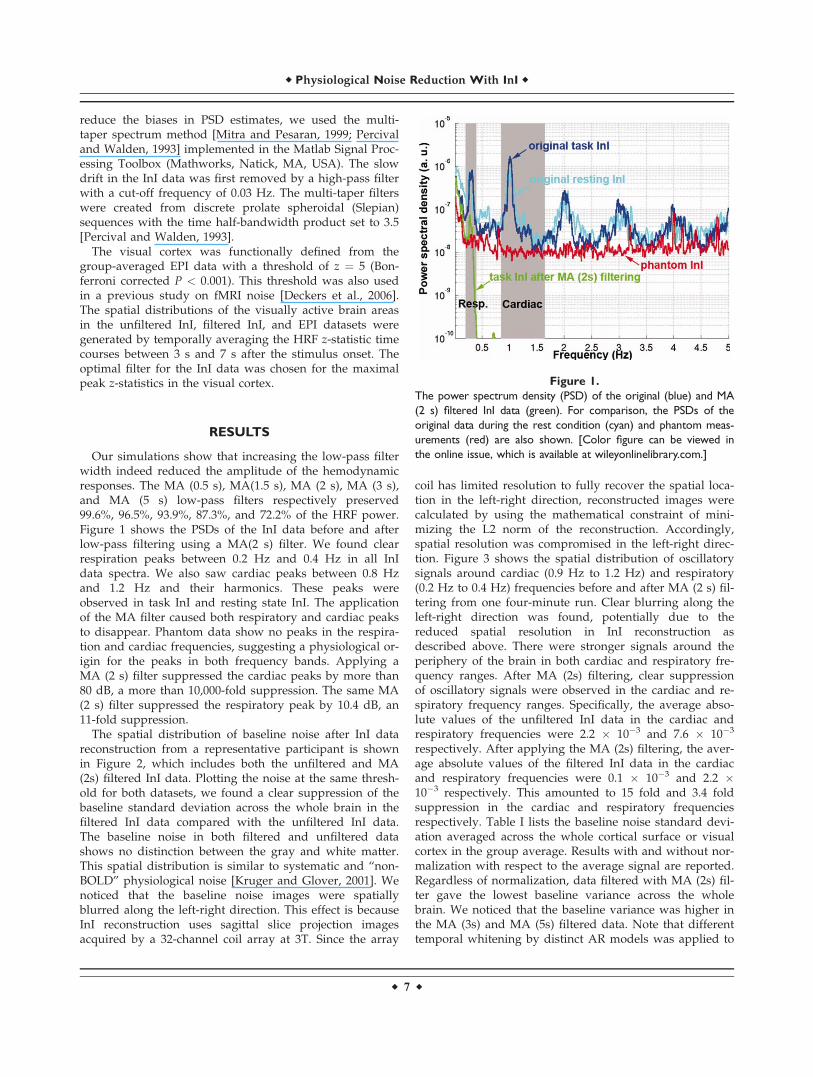
Our simulations show that increasing the low-pass filterwidth indeed reduced the amplitude of the hemodynamicresponses. The MA (0.5 s), MA(1.5 s), MA (2 s), MA (3 s),and MA (5 s) low-pass filters respectively preserved99.6%, 96.5%, 93.9%, 87.3%, and 72.2% of the HRF power.Figure 1 shows the PSDs of the InI data before and afterlow-pass filtering using a MA(2 s) filter. We found clearrespiration peaks between 0.2 Hz and 0.4 Hz in all InIdata spectra. We also saw cardiac peaks between 0.8 Hzand 1.2 Hz and their harmonics. These peaks wereobserved in task InI and resting state InI. The applicationof the MA filter caused both respiratory and cardiac peaksto disappear. Phantom data show no peaks in the respira-tion and cardiac frequencies, suggesting a physiological or-igin for the peaks in both frequency bands. Applying aMA (2 s) filter suppressed the cardiac peaks by more than80 dB, a more than 10,000-fold suppression. The same MA(2 s) filter suppressed the respiratory peak by 10.4 dB, an11-fold suppression.

The spatial distribution of baseline noise after InI datareconstruction from a representative participant is shownin Figure 2, which includes both the unfiltered and MA(2s) filtered InI data. Plotting the noise at the same thresh-old for both datasets, we found a clear suppression of thebaseline standard deviation across the whole brain in thefiltered InI data compared with the unfiltered InI data.The baseline noise in both filtered and unfiltered datashows no distinction between the gray and white matter.This spatial distribution is similar to systematic and ‘‘non-BOLD’’ physiological noise [Kruger and Glover, 2001]. Wenoticed that the baseline noise images were spatiallyblurred along the left-right direction. This effect is becauseInI reconstruction uses sagittal slice projection imagesacquired by a 32-channel coil array at 3T. Since the array

coil has limited resolution to fully recover the spatial loca-tion in the left-right direction, reconstructed images werecalculated by using the mathematical constraint of mini-mizing the L2 norm of the reconstruction. Accordingly,spatial resolution was compromised in the left-right direc-tion. Figure 3 shows the spatial distribution of oscillatorysignals around cardiac (0.9 Hz to 1.2 Hz) and respiratory(0.2 Hz to 0.4 Hz) frequencies before and after MA (2 s) fil-tering from one four-minute run. Clear blurring along theleft-right direction was found, potentially due to thereduced spatial resolution in InI reconstruction asdescribed above. There were stronger signals around theperiphery of the brain in both cardiac and respiratory fre-quency ranges. After MA (2s) filtering, clear suppressionof oscillatory signals were observed in the cardiac and re-spiratory frequency ranges. Specifically, the average abso-lute values of the unfiltered InI data in the cardiac andrespiratory frequencies were 2.2 " 10(3 and 7.6 " 10(3

respectively. After applying the MA (2s) filtering, the aver-age absolute values of the filtered InI data in the cardiacand respiratory frequencies were 0.1 " 10(3 and 2.2 "10(3 respectively. This amounted to 15 fold and 3.4 foldsuppression in the cardiac and respiratory frequenciesrespectively. Table I lists the baseline noise standard devi-ation averaged across the whole cortical surface or visualcortex in the group average. Results with and without nor-malization with respect to the average signal are reported.Regardless of normalization, data filtered with MA (2s) fil-ter gave the lowest baseline variance across the wholebrain. We noticed that the baseline variance was higher inthe MA (3s) and MA (5s) filtered data. Note that differenttemporal whitening by distinct AR models was applied to

Figure 1.The power spectrum density (PSD) of the original (blue) and MA(2 s) filtered InI data (green). For comparison, the PSDs of theoriginal data during the rest condition (cyan) and phantom meas-urements (red) are also shown. [Color figure can be viewed inthe online issue, which is available at wileyonlinelibrary.com.]

r Physiological Noise Reduction With InI r

r 7 r

Figure 3.The spatial distribution of noise in cardiac (0.9–1.2 Hz) and respiratory (0.2–0.4 Hz) frequencyranges. Axial slice images are shown without filtering and with MA (2 s) filtering. The color enc-odes the standard deviation of the noise in arbitrary units. [Color figure can be viewed in theonline issue, which is available at wileyonlinelibrary.com.]

Figure 2.The spatial distribution of baseline noise estimated from the residuals in the GLM model. Axialslice images are shown without filtering and with MA (2 s) filtering. The color encodes thestandard deviation of the noise in arbitrary units. [Color figure can be viewed in the online issue,which is available at wileyonlinelibrary.com.]

r Lin et al. r

r 8 r

the time series to ensure efficient estimation of hemody-namic responses with correct degrees of freedom. Thisstep is likely to generate different estimates of baselinenoise variance. In addition, using a long smoothing win-dow may temporally smear the BOLD signal into baselinetime points and consequently lead to over estimation ofbaseline fluctuation. Since baseline noise was not esti-mated from the moving average of unfiltered hemody-namic response, we did not observe a monotonic decreaseof baseline variance.

Figure 4 shows the snapshots of unfiltered InI data and2 s MA filtered InI data from a representative participant.These snapshots show dynamic activation of the visualcortex with reasonable localization. 2 s MA filtered InIshows higher z statistics. Interestingly the 2 s MA filteredInI results show subcortical activity with dynamics similarto cortical BOLD responses. This may be the mis-localizedhemodynamic response at the lateral geniculate nucleusdue to highly ill-conditioned encoding matrix at the deepbrain area.

The visual cortex HRFs for unfiltered InI data, 2 s MA fil-tered InI data, and spatially smoothed EPI (FWHM ¼ 8.6mm) data from a representative participant and the entiregroup are in Figure 5. The visual cortex average time coursereaches its peak value about the same time in the unfilteredInI, filtered InI, and smoothed EPI data. Although the peaklatencies vary between EPI and InI data. it is difficult tomake strong inferences about these differences, due to thetemporal resolution difference between EPI (TR ¼ 2 s) andInI (TR ¼ 0.1 s) acquisitions,. Compared to the unfilteredInI data and smoothed EPI data, we found that MA filter-ing of the InI data improved the detection sensitivity, asevidenced by a higher z-statistic peak value in the visualcortex. For the single participant and the group average,MA (2s) low-pass filtered InI results have higher peak z-sta-tistic values of 39.5 and 34.3 compared to either the unfil-tered InI data with peak values of 17.5 and 21.8 or thesmoothed EPI data with peak values of 25.1 and 21.7. Com-pared to unfiltered InI and spatially smoothed EPI (FWHM¼ 8.6 mm), MA (2 s) filtering improved the peak z-statisticsby 126% and 57% for this representative participant and57% and 58% for the group. The InI and EPI peak values inthe visual cortex for each participant and the group averageare listed in Tables II and III.

Figure 6 shows the spatial distribution of the z-statisticsaveraged between 3 and 7 s after stimulus onset froma representative participant and the group average. For

comparison, the EPI data spatially smoothed by a FWHM¼ 8.6 mm kernel are also shown rendered on the inflatedcortical surfaces. The location of visual cortex is wellmatched in the unfiltered InI, filtered InI, and smoothedEPI conditions. Compared with the original InI data,applying a MA (2 s) filter increased the visual cortex peakz-statistic in both the single participant and the group av-erage (Tables II and III).

Snapshots of visual cortex activity for the group aver-age data are shown in Figure 7. Greater spatial extentand increased task-related activity duration were seen inthe filtered InI data. Compared with the filtered InI datausing a MA (2 s) filter with a z ¼ 5 critical threshold, alater detection of suprathreshold activity was observedin the absence of filtering. Unfiltered InI data showedthe suprathreshold visual cortex activity at approxi-mately 2.3 s after the visual stimulus onset, while fil-tered InI data using a MA (2 s) filter showed thesuprathreshold visual cortex activity at ) 1.7 s after thevisual stimulus onset. The localization of the visual cor-tex, however, is very consistent between filtered andunfiltered InI data.

The MA (2 s) low-pass filter was originally chosen tomatch TRs commonly used in multi-slice EPI acquisition.We expected variations in the moving average filter dura-tions to influence detection sensitivity. The results of thegroup z-statistic average time courses in visual cortex areshown in Figure 8. We found that the task-related activ-ity peaks progressively increase when the moving aver-age filter window increases from 0.5 s to 2 s. Furtherincreases in the filter window decrease the observedeffects. This pattern has two likely explanations. First, thefailure of a short moving average window to effectivelysuppress oscillatory fluctuations, such as cardiac artifacts,may result in decreased contrast-to-noise ratios and con-sequent reduced sensitivity to task-related activity. Sec-ond, a longer moving average window can suppress notonly cardiac and respiratory fluctuations but also func-tional contrast. Thus, an excessively long moving averagewindow can result in an overall CNR decrease. Weobserved small peak latency differences between hemody-namic responses estimated from filtered InI data com-pared to estimates derived from unfiltered InI data orEPI data. This effect may be due to differential tempo-rally whitening associated with different AR modelsemployed in order to achieve efficient estimation ofhemodynamic responses with the correct degrees of

TABLE I. Baseline standard deviation of the InI data with and without normalization to the average signal averagedacross the entire cortex and within the visual cortex in the group analysis

Unfiltered MA (0.5 s) MA (1.5 s) MA (2 s) MA (3 s) MA (5 s)

Without normalization Entire cortex ("10(5) 9.7 6.4 4.2 3.8 4.5 6.7Visual cortex ("10(5) 12.0 8.9 4.9 4.2 5.3 8.5

With normalization Entire cortex ("10(3) 12.4 8.3 5.3 4.8 5.8 8.6Visual cortex ("10(3) 11.5 9.6 5.3 4.3 5.7 9.6

r Physiological Noise Reduction With InI r

r 9 r

freedom. This step is likely to effect the estimated hemo-dynamic response shapes and to lead to differentobserved latencies.

Since InI has anisotropic spatial resolution [Lin et al.,2008a; Lin et al., 2008b], we also compared filtered InI dataand spatially smoothed EPI data using different smoothingkernels (Fig. 9). Compared to unsmoothed EPI data,smoothing the EPI data using kernels of FWHM ¼ 3 mmand FWHM ¼ 4.7 mm resulted in increased sensitivity to

visual cortex activity. The largest peak statistics werefound after smoothing EPI data using a kernel of FWHM¼ 8.6 mm. Further increasing the width of the smoothingkernel to 12 or 18 mm reduces the detection sensitivity.However, temporally filtered InI data using a MA (2 s) fil-ter has a peak z- statistic of 34.3, while the highest peak z-statistic in the spatially smoothed EPI data resulting fromapplication of a FWHM ¼ 8.6 mm kernel of was only 21.7(Tables II and 3).

Figure 4.Time series of the volumetric reconstruction of unfiltered InI and filtered InI using a MA 2s filterfrom a representative participant. The critical threshold was z ¼ 4. [Color figure can be viewedin the online issue, which is available at wileyonlinelibrary.com.]

r Lin et al. r

r 10 r

Figure 5.The average time course for a representative participant (left) and the group (right) in the visualcortex before (black trace) and after (blue trace) filtering using a MA (2 s) filter. EPI timecourses (red traces) are shown for comparison. [Color figure can be viewed in the online issue,which is available at wileyonlinelibrary.com.]

TABLE II. InI peak z-statistics in the visual cortex before and after moving-average filtering

Participant Unfiltered InI

Temporally filtered InI

MA (0.5s) MA (1.5s) MA (2s) MA (3s) MA (5s)

1 17.5 25.1 26.7 39.5 21.5 22.02 10.1 5.8 7.2 9.3 5.8 2.63 9.1 8.8 9.0 11.2 7.9 6.64 5.8 5.0 12.0 13.8 11.7 8.35 14.8 8.7 13.0 23.1 15.6 13.26 9.8 12.4 15.3 15.7 14.6 11.1Average 21.8 18.7 29.1 34.3 25.3 17.4

TABLE III. EPI peak z-statistics in the visual cortex before and after spatial smoothing

Participant Unsmoothed EPI

Spatially smoothed EPI

FWHM.3.0 mm FWHM 4.7 mm FWHM 8.6 mm FWHM 12 mm FWHM 18 mm

1 9.2 9.9 14.3 25.1 18.9 20.82 10.7 14.3 22.4 34.3 18.1 16.23 8.2 8.5 10.9 11.3 6.3 5.24 7.4 8.8 8.7 10.1 2.9 2.15 12.6 13.2 16.7 20.0 18,3 17.96 1.9 2.2 1.9 2.2 2.1 2.1Average 4.5 14.8 15.8 21.7 12.6 11.9

r Physiological Noise Reduction With InI r

r 11 r

DISCUSSION

BOLD-contrast magnetic resonance inverse imagingallows indirect detection of neural activity changes, withan order-of-magnitude advantage in temporal resolutionwhen compared to standard EPI methods for whole-brainstudies. In addition to its ability to identify the fine tempo-ral features of the hemodynamic response, InI allows useof digital processing methods for suppressing physiologi-cal noise sources without the need for external physiologi-cal monitoring devices. In the group average data, thebaseline standard deviation in visual cortex in the tempo-rally filtered InI data with a MA (2 s) filter is 39% of theunfiltered InI data (Fig. 2 and Table I). In visual cortex, thebaseline standard deviation in the temporally filtered InIdata with a MA (2 s) filter is 35% of the unfiltered InI data(Fig. 2 and Table I). The maximal z-statistic in visual cortexincreased from 21.8 in the unfiltered InI data to 34.3 in thefiltered InI data (MA (2 s) filter, a 57% increase (Fig. 3,Tables II and III). Compared to spatially smoothed EPIdata (FWHM ¼ 8.6 mm), the filtered InI data has a 58%higher peak z-value (Fig. 3, Tables II and III). This result ishigher than the 4% increase observed when using adaptivefiltering, which has comparable performance to that seenwith the RETROICOR method [Deckers et al., 2006]. Theadvantages InI provides in suppressing physiological noiseinclude increased detection sensitivity in all InI fMRI

Figure 7.Time series of unfiltered and filtered InI cortical activity reconstructions in the visual cortex inresponse to visual stimulation from a group of six participants. The critical threshold was z ¼ 5.[Color figure can be viewed in the online issue, which is available at wileyonlinelibrary.com.]

Figure 6.A medial view of the inflated left hemisphere cortex overlaid withthe z-statistic maps showing the spatial distribution of the activevisual cortex before and after MA (2 s) filtering compared to theEPI data smoothed with a 8.6 mm FWHM kernel in single partici-pant (top panel) and group (bottom panel). The dark and light grayindicate sulci and gyri, respectively. [Color figure can be viewed inthe online issue, which is available at wileyonlinelibrary.com.]

r Lin et al. r

r 12 r

experiments. Our filtering approach can also aid in detect-ing subtle changes in response timing within brain areasacross task conditions. When comparing timing differencesat a particular brain location, there are no confoundinginfluences contributed by differential vasculature effectsand therefore the timing difference between conditions canmore easily be attributed to changes in neural activity.

In contrast to many previously described techniques forreducing the effects of physiological noise, InI filteringdoes not require an external cardiac or respiratory moni-toring device to directly record cardiac and respiratory ac-tivity that, when undersampled in the temporal domain,can lead to aliased noised. External monitoring devicescan collect cardiac and respiratory signals that can beused to create nuisance-variable regressors [Birn et al.,2006; Lund et al., 2006] to remove periodic, low-frequency(<0.1 Hz) sources of physiological noise. However, thereis an unknown latency between these peripherally moni-tored signals and their associated brain signals. Theperipheral to central latency can also vary due to spatialvariations in neurovascular coupling. Physiologically, pul-sations of cardiac or respiratory origin have dominant fre-quencies around 1.0 and 0.25 Hz respectively. Both noisesources are relatively broadband because of the intrinsicvariability in autonomic nervous system modulation andthe mutual interaction between the competing sympatheticand parasympathetic influences. Using standard EPI acqui-sition techniques, while it is possible to monitor and sub-sequently reduce low-frequency (<0.1 Hz) CO2-mediatedphysiological noise [Birn et al., 2006; Shmueli et al., 2007;Wise et al., 2004], it is more difficult to remove the effects

of respiratory and cardiac fluctuations due to samplingrate limitations. While it usually takes up to 2 s to com-plete an EPI volumetric acquisition with whole-brain cov-erage, the required sampling period to avoid cardiac noisealiasing based on the Nyquist sampling theorem is 0.5 s orless. InI can avoid this problem by achieving whole-brainacquisition with sampling intervals as short as 0.1 s usingRF encoding.

Because of the ill-posed nature of raw InI data, thereexist different alternatives for InI image reconstruction,including minimum L2 norm [Lin et al., 2008a], spatial fil-tering [Lin et al., 2008b], or k-space techniques [Lin et al.,2010]. However, the utility of the filtering method exam-ined in this paper is not dependent on any specific imagereconstruction algorithm. Physiological noise can first besuppressed using digital filtering, after which a particularreconstruction algorithm can be chosen. Therefore, digitalfiltering can be considered as a pre-processing step withbenefits independent of particular reconstruction methods.

In this study, we used temporal filters to reduce theeffects of cardiac and respiratory noise. While other digitalfiltering techniques can be used to suppress these noisesources, moving average filters are computationally effi-cient and extremely easy to implement. Theoretically, theuse of MA filters can result in passband ringing. However,our results did not show significant ringing artifacts in thespectral (Fig. 1) or temporal (Fig. 5) domains. One disad-vantage of employing a moving average filter is that the

Figure 8.The averaged z-statistic time course in the visual cortex usingunfiltered InI data (solid cyan) and InI data filtered by differentmoving average filters. InI data filtered with the MA (2 s) filter(solid blue) results in the maximal peak z-statistic value. [Colorfigure can be viewed in the online issue, which is available atwileyonlinelibrary.com.]

Figure 9.The averaged z-statistic time course in the visual cortex usingsmoothed EPI data (solid red) and EPI data spatially smoothedby kernels with different widths. Among all EPI data, EPIsmoothed by a kernel FWHM ¼ 8.6 mm (solid magenta) hasthe maximal peak z-statistic value. InI data filtered with the MA(2 s) filter (solid blue) has a even larger peak z-statistic. [Colorfigure can be viewed in the online issue, which is available atwileyonlinelibrary.com.]

r Physiological Noise Reduction With InI r

r 13 r

low-pass filtering does indeed increase the temporal corre-lation among the elements of a time series. Therefore,studies concerned with very transient fMRI responses maytherefore benefit from the use of other filtering methods toreduce cardiac and respiratory noise without distorting thefine temporal structure of the task-related responses. Forexample, adaptive filtering methods have been applied inoptical imaging to reduce global signal variation [Zhanget al., 2007]. In theory, these methods can be applied to InIdata to reduce physiological noise while preserving thetemporal structure of transient signal changes.

The physiological noise sources that have been the focusof our study mostly originate from cyclic cardiac and respi-ratory activity. We assume that these artifacts have quasi-periodic waveforms and that the sampling rate of volumet-ric inverse imaging is sufficiently fast to avoid temporalnoise aliasing. The current implementation of volumetricInI uses 100 ms temporal resolution for whole-brain cover-age. This sampling frequency, in typical physiological con-ditions, is sufficiently high to meet the Nyquist samplingcriterion. The cost associated with the high InI samplingrate is a loss of spatial resolution, since InI solves underde-termined linear systems in image reconstructions. Due tothe ill posed nature of these underdetermined linear sys-tems, there exist an infinite number of solutions. However,imposing constraints can allow solution of underdeter-mined linear systems. We previously investigated the useof minimum L2 norm solutions [Lin et al., 2008a] and spa-tial filtering techniques using linear constraint minimumvariance beamformers [Lin et al., 2008b]. Depending on theSNR of the measurements, it is possible to obtain an aver-age point spread function of 8.6, 4.7, and 3.0 mm in mini-mum L2 norm reconstructions at SNRs of 10, 5, and 1,respectively. Since fMRI data collected using EPI acquisi-tion methods usually involves spatial smoothing toimprove the SNR [Friston, 2007], a small loss of spatial re-solution is generally considered acceptable. Note that if theLCMV beamformer is used as an alternative reconstructionalgorithm for InI data, the average point spread function isusually below 1 mm [Lin et al., 2008b]. In this case, theloss of spatial resolution may be negligible.

We found that Figures 2, 3, and 4 were not perfectly sym-metric along the left-right direction. Note that these figuresare results of functional activity rather than anatomy. Thuswe cannot completely attribute asymmetric appearance tothe reconstruction. Notably, Figure 4 is the result from onesingle subject. And there have been reports on the variabili-ty of visual cortex BOLD responses [de Zwart et al., 2005;Handwerker et al., 2004], which might explain why theobserved visual cortex activity is not 100% symmetric evensymmetric stimuli were presented.

InI indeed has intrinsic a spatial smoothing effect as theresult of using the constraint of minimizing the L-2 normof the reconstruction. Such smoothing can improve the sig-nal-to-noise ratio and it is spatially variying [Lin et al.,2010; Lin et al., 2008a; Lin et al., 2008b]. Considering thecommon EPI processing stream using only one homogene-ous 3D smoothing kernel, a fair comparison, in our mind,

would be spatially smoothing InI and EPI such that theaverage cortical resolution is comparable. This is in factwhat we did. Even considering different spatial smoothingeffects in InI reconstructions, Figure 8 clearly shows thatEPI data using different spatially smoothing kernels(FWHM ¼ 3 mm to 18 mm) do not generate as high statis-tics as temporally smoothed InI data. Taken together, spa-tial smoothing in InI is not dominating the SNRimprovement in BOLD fMRI time series. The suppressionof the fluctuation in InI time also contributes significantlyto the overall improvement in the sensitivity of BOLDhemoydnamic responses detection.

Cardiac and respiratory periodic modulations are part ofthe ‘‘non-BOLD’’ component of physiological temporalnoise (rNB) [Kruger and Glover, 2001]. The other type ofphysiological temporal noise is similar to BOLD-contrastsignal (rB), whose magnitude depends on TE of the mea-surement [Kruger and Glover, 2001]. rNB noise has a morehomogenous spatial distribution, while rB noise is higherin gray matter than white matter [Kruger and Glover,2001]. With TR ¼ 3 s, the ratio between rNB and rB noiseat 3T is ) 1:2, implying that our temporal filtering methodcan optimally reduce physiological noise by 33%. Note thatthese numbers depend on TE, flip angle [Gonzalez-Castillo,2010], and TR. To further reduce the rB physiological noise,we may look to other solutions. It has been suggested thatsampling with high spatial resolution and subsequentlysmoothing the data along the gray matter can effectivelyreduce the rB physiological noise [Triantafyllou et al.,2006]. This is due to the fact that physiological noise sour-ces are partially spatially correlated. Sampling at higherspatial resolution can ensure that the noise sources aredominated by thermal, rather than physiological, noise.Subsequent spatial smoothing of thermal noise dominateddata can compensate for the loss of signal without loweringthe SNR, since thermal noise is spatially uncorrelated.Increasing spatial resolution to reduce the relative contribu-tion of physiological noise reduces the advantage of InI ascompared with EPI. However, if we know a priori that therB noise is less concentrated in a specific k-space region, assuggested by [Bodurka et al., 2007; Lowe and Sorenson,1997], then InI accelerated scans can be acquired in thatspecific k-space region in order to reduce physiologicalnoise contamination. Namely, instead of acquiring projec-tion images (kz ¼ 0) in InI, we can also acquire k-space datacorresponding to a spatial harmonic (kz = 0) in acceleratedInI acquisition. Hypothetically, the reconstructed volumetricimages can have reduced physiological noise.

It has been suggested that a steady state free precession(SSFP) signal can develop under a train of RF pulses withTR < T2 in single-shot EPI [Zhao et al., 2000]. B0 fluctua-tions originating from respiration, physical movement out-side the FOV, and system instability can cause SSFPtemporal variation. InI uses a brief TR ¼ 100 ms and thusthis mechanism can potentially contribute to time seriesvariation. It has been suggested that a strong crusher canbe used to minimize these temporal noise fluctuations

r Lin et al. r

r 14 r

[Zhao et al., 2000]. In fact, our experiment used a crushergradient of 20 mT/m strength and 10-ms duration, as pre-viously suggested [Zhao et al., 2000]. However, since thesuggested strong crusher was studied with TR ¼ 200 ms,InI may require further increase the crusher moment toreduce the SSFP signal disturbance by increasing thecrusher duration or strength. However, the potential costwill be reduced temporal resolution and more prominenteddy current artifacts.

In conclusion, the high sampling rate made possible withMR InI can be exploited to monitor and suppress cardiacand respiratory physiological noise sources without theneed for external monitoring devices. We systematicallyinvestigated this advantage by parametrically modulatingthe temporal filtering parameters and then comparing theresults to EPI acquisitions processed with different spatialsmoothing kernels. The improved detection power afterphysiological noise suppression was validated across par-ticipants and the improvements resulting from noise sup-pression are strong and statistically significant. The InImethod can be used in BOLD-contrast fMRI experimentsusing parallel detection from a RF coil array to furtherimprove the sensitivity of detecting localized changes inneural activity that are either spontaneous, as in restingstate studies, or task-related, as in investigations of the neu-ral mechanisms of perception, cognition and action.

REFERENCES

Barry RL, Menon RS (2005): Modeling and suppression of respira-tion-related physiological noise in echo-planar functional mag-netic resonance imaging using global and one-dimensionalnavigator echo correction. Magn Reson Med 54:411–418.

Birn RM, Diamond JB, Smith MA, Bandettini PA (2006): Separa-ting respiratory-variation-related fluctuations from neuronal-ac-tivity-related fluctuations in fMRI. Neuroimage 31:1536–1548.

Biswal B, DeYoe AE, Hyde JS (1996): Reduction of physiologicalfluctuations in fMRI using digital filters. Magn Reson Med35:107–113.

Bodurka J, Ye F, Petridou N, Murphy K, Bandettini PA (2007):Mapping the MRI voxel volume in which thermal noisematches physiological noise–implications for fMRI. Neuro-image 34:542–549.

Brainard DH (1997): The Psychophysics Toolbox. Spat Vis 10(4),433–436.

Cox RW, Jesmanowicz A (1999): Real-time 3D image registrationfor functional MRI. Magn Reson Med 42:1014–1018.

Dagli MS, Ingeholm JE, Haxby JV (1999): Localization of cardiac-induced signal change in fMRI. Neuroimage 9:407–415.

Dale AM, Fischl B, SerenoMI (1999): Cortical surface-based analysis.I. Segmentation and surface reconstruction. Neuroimage 9:179–194.

Dale AM, Liu AK, Fischl BR, Buckner RL, Belliveau JW, LewineJD, Halgren E (2000): Dynamic statistical parametric mapping:Combining fMRI and MEG for high-resolution imaging of cort-ical activity. Neuron 26:55–67.

de Zwart JA, Silva AC, van Gelderen P, Kellman P, Fukunaga M,Chu R, Koretsky AP, Frank JA, Duyn JH (2005): Temporal dy-namics of the BOLD fMRI impulse response. Neuroimage24:667–677.

Deckers RH, van Gelderen P, Ries M, Barret O, Duyn JH, Ikono-midou VN, Fukunaga M, Glover GH, de Zwart JA (2006): Anadaptive filter for suppression of cardiac and respiratory noisein MRI time series data. Neuroimage 33:1072–1081.

Feinberg DA (1992): Modern concepts of brain motion and cere-brospinal fluid flow. Radiology 185:630–632.

Feinberg DA, Mark AS (1987): Human brain motion and cerebro-spinal fluid circulation demonstrated with MR velocity imag-ing. Radiology 163:793–799.

Fischl B, Sereno MI, Dale AM. (1999a): Cortical surface-basedanalysis. II: Inflation, flattening, and a surface-based coordinatesystem. Neuroimage 9:195–207.

Fischl B, Sereno MI, Tootell RB, Dale AM. (1999b): High-resolutionintersubject averaging and a coordinate system for the corticalsurface. Hum Brain Mapp 8:272–284.

Friston KJ.2007. Statistical Parametric Mapping: The Analysis ofFuntional Brain Images. Amsterdam: Boston: Elsevier/Aca-demic Press. vii, 647 p.

Glover GH (1999): Deconvolution of impulse response in event-related BOLD fMRI. Neuroimage 9:416–429.

Glover GH, Li TQ, Ress D (2000): Image-based method for retro-spective correction of physiological motion effects in fMRI:RETROICOR. Magn Reson Med 44:162–167.

Gonzalez-Castillo J, Roopchansingh V, Bandettini PA, Bodurka J(2010): Physiological noise effects on the flip angle selection inBOLD fMRI. Neuroimage 54:2764–2778.

Hajnal JV, Myers R, Oatridge A, Schwieso JE, Young IR, BydderGM (1994): Artifacts due to stimulus correlated motion infunctional imaging of the brain. Magn Reson Med 31:283–291.

Handwerker DA, Ollinger JM, D’Esposito M (2004): Variation ofBOLD hemodynamic responses across subjects and brainregions and their effects on statistical analyses. Neuroimage21:1639–1651.

Hennig J, Zhong K, Speck O (2007): MR-Encephalography: Fastmulti-channel monitoring of brain physiology with magneticresonance. Neuroimage 34:212–219.

Hu X, Kim SG (1994): Reduction of signal fluctuation in functionalMRI using navigator echoes. Magn Reson Med 31:495–503.

Hu X, Le TH, Parrish T, Erhard P (1995): Retrospective estimationand correction of physiological fluctuation in functional MRI.Magn Reson Med 34:201–212.

Kruger G, Glover GH (2001): Physiological noise in oxygenation-sensitive magnetic resonance imaging. Magn Reson Med46:631–637.

Kwong KK, Belliveau JW, Chesler DA, Goldberg IE, WeisskoffRM, Poncelet BP, Kennedy DN, Hoppel BE, Cohen MS, TurnerR, et al. (1992): Dynamic magnetic resonance imaging ofhuman brain activity during primary sensory stimulation. ProcNatl Acad Sci USA 89:5675–5679.

Lin FH, Wald LL, Ahlfors SP, Hamalainen MS, Kwong KK, Belli-veau JW (2006): Dynamic magnetic resonance inverse imagingof human brain function. Magn Reson Med 56:787–802.

Lin FH, Witzel T, Chang WT, Wen-Kai Tsai K, Wang YH, KuoWJ, Belliveau JW (2010): K-space reconstruction of magneticresonance inverse imaging (K-InI) of human visuomotor sys-tems. Neuroimage 49:3086–3098.

Lin FH, Witzel T, Mandeville JB, Polimeni JR, Zeffiro TA, GreveDN, Wiggins G, Wald LL, Belliveau JW (2008a): Event-relatedsingle-shot volumetric functional magnetic resonance inverseimaging of visual processing. Neuroimage 42:230–247.

Lin FH, Witzel T, Zeffiro TA, Belliveau JW (2008b): Linear con-straint minimum variance beamformer functional magneticresonance inverse imaging. Neuroimage 43:297–311.

r Physiological Noise Reduction With InI r

r 15 r

Logothetis NK, Pauls J, Augath M, Trinath T, Oeltermann A(2001): Neurophysiological investigation of the basis of thefMRI signal. Nature 412:150–157.

Lowe MJ, Sorenson JA (1997): Spatially filtering functional magneticresonance imaging data. Magn ResonMed 37:723–729.

Lund TE, Madsen KH, Sidaros K, Luo WL, Nichols TE (2006):Non-white noise in fMRI: Does modelling have an impact?Neuroimage 29:54–66.

McDougall MP, Wright SM (2005): 64-channel array coil for single echoacquisitionmagnetic resonance imaging.MagnResonMed 54:386–392.

Mistretta CA, Wieben O, Velikina J, Block W, Perry J, Wu Y, John-son K, Wu Y (2006): Highly constrained backprojection fortime-resolved MRI. Magn Reson Med 55:30–40.

Mitra PP, Pesaran B (1999): Analysis of dynamic brain imagingdata. Biophys J 76:691–708.

Neumaier A, Schneider T (2001): Estimation of parameters andeigenmodes of multivariate autoregressive models. ACMTrans. Math Softw 27:27–57.

Ogawa S, Lee TM, Kay AR, Tank DW (1990): Brain magnetic reso-nance imaging with contrast dependent on blood oxygenation.Proc Natl Acad Sci USA 87:9868–9872.

Pelli DG (1997): The VideoToolbox software for visual psycho-physics: transforming numbers into movies. Spat Vis 10:437–442.

Percival DB, Walden AT (1993): Spectral Analysis for Physical Appli-cations: Multitaper and Conventional Univariate Techniques. Cam-bridge, New York, NY: Cambridge University Press. xxvii, 583 p.

Pfeuffer J, Van de Moortele PF, Ugurbil K, Hu X, Glover GH(2002): Correction of physiologically induced global off-reso-nance effects in dynamic echo-planar and spiral functionalimaging. Magn Reson Med 47:344–353.

Poncelet BP, Wedeen VJ, Weisskoff RM, Cohen MS (1992): Brainparenchyma motion: Measurement with cine echo-planar MRimaging. Radiology 185:645–651.

Pruessmann KP, Weiger M, Scheidegger MB, Boesiger P (1999):SENSE: Sensitivity encoding for fast MRI. Magn Reson Med42:952–962.

Purdon PL, Weisskoff RM (1998): Effect of temporal autocorrelationdue to physiological noise and stimulus paradigm on voxel-levelfalse-positive rates in fMRI. Hum Brain Mapp 6:239–249.

Schneider T, Neumaier A (2001): Algorithm 808: ARfit - A Matlabpackage for the estimation of parameters and eigenmodes ofmultivariate autoregressive models. ACM Trans Math Softw27:58–65.

Shmueli K, van Gelderen P, de Zwart JA, Horovitz SG, FukunagaM, Jansma JM, Duyn JH (2007): Low-frequency fluctuations inthe cardiac rate as a source of variance in the resting-statefMRI BOLD signal. Neuroimage 38:306–320.

Sodickson DK, Manning WJ (1997): Simultaneous acquisition ofspatial harmonics (SMASH): Fast imaging with radiofrequencycoil arrays. Magn Reson Med 38:591–603.

Thomas CG, Harshman RA, Menon RS (2002): Noise reduction inBOLD-based fMRI using component analysis. Neuroimage17:1521–1537.

Triantafyllou C, Hoge RD, Wald LL (2006): Effect of spatialsmoothing on physiological noise in high-resolution fMRI.Neuroimage 32:551–557.

Windischberger C, Langenberger H, Sycha T, Tschernko EM,Fuchsjager-Mayerl G, Schmetterer L, Moser E (2002): On theorigin of respiratory artifacts in BOLD-EPI of the human brain.Magn Reson Imaging 20:575–582.

Wise RG, Ide K, Poulin MJ, Tracey I (2004): Resting fluctuations inarterial carbon dioxide induce significant low frequency varia-tions in BOLD signal. Neuroimage 21:1652–1664.

Woods RP, Grafton ST, Holmes CJ, Cherry SR, Mazziotta JC(1998): Automated image registration. I. General methods andintrasubject, intramodality validation. J Comput Assist Tomogr22:139–152.

Worsley KJ, Liao CH, Aston J, Petre V, Duncan GH, Morales F,Evans AC (2002): A general statistical analysis for fMRI data.Neuroimage 15:1–15.

Zhang Q, Brown EN, Strangman GE. (2007)Adaptive filteringto reduce global interference in evoked brain activitydetection: A human subject case study. J Biomed Opt 12:064009.

Zhao X, Bodurka J, Jesmanowicz A, Li SJ (2000): B(0)-fluctuation-induced temporal variation in EPI image series due to the dis-turbance of steady-state free precession. Magn Reson Med44:758–765.

r Lin et al. r

r 16 r