Helsinki University of Technology  Laboratory of Acoustics and Audio Signal ProcessingEspoo 2007 Report 85

PHYSICS­BASED PARAMETRIC SYNTHESIS OFINHARMONIC PIANO TONES

Jukka Rauhala

Dissertation for the degree of Doctor of Science in Technology to be presented with duepermission for public examination and debate in Auditorium S4, Department of Electricaland Communications Engineering, Helsinki University of Technology, Espoo, Finland,  onthe 14th of December 2007, at 12 o'clock noon.

Helsinki University of TechnologyDepartment of Electrical and Communications EngineeringLaboratory of Acoustics and Audio Signal Processing

Teknillinen korkeakouluSähkö­ ja tietoliikennetekniikan osastoAkustiikan ja äänenkäsittelytekniikan laboratorio

Helsinki University of TechnologyLaboratory of Acoustics and Audio Signal ProcessingP.O. Box 3000FIN­02015 TKKTel. +358 9 4511Fax +358 9 460 224E­mail lea.soderman@tkk.fiISBN 978­951­22­9065­9ISSN 1456­6303

Multiprint OyEspoo, Finland 2007

ABABSTRACT OF DOCTORAL DISSERTATION HELSINKI UNIVERSITY OF TECHNOLOGY

P. O. BOX 1000, FI-02015 TKK

http://www.tkk.fi

Author Jukka Rauhala

Name of the dissertation

Manuscript submitted 13.8.2007 Manuscript revised 2.11.2007

Date of the defence 14.12.2007

Article dissertation (summary + original articles)Monograph

Department

Laboratory

Field of research

Opponent(s)

Supervisor

Instructor

Abstract

Keywords acoustic signal processing, digital signal processing, music

ISBN (printed) 978-951-22-9065-9

ISBN (pdf) 978-951-22-9066-6

Language English

ISSN (printed) 1456-6303

ISSN (pdf)

Number of pages 155

Publisher Helsinki University of Technology, Laboratory of Acoustics and Audio Signal Processing

Print distribution Report 85 / TKK, Laboratory of Acoustics and Audio Signal Processing, Espoo, Finland

The dissertation can be read at http://lib.tkk.fi/Diss/

Physics-based parametric synthesis of inharmonic piano tones

X

Department of Electrical and Communications Engineering

Laboratory of Acoustics and Audio Signal Processing

Audio signal processing

Professor Augusto Sarti

Professor Vesa Välimäki

Professor Vesa Välimäki

X

This dissertation studies methods for developing a parametric piano synthesis model using the physics-based approach.The goal is to develop a model that can be controlled with physically meaningful parameters. Moreover, the model isrequired to be computationally efficient for real-time implementation. The basis of this work is to use the digitalwaveguide technique for implementing a piano string model. The excitation signal, simulation of dispersion, thebeating effect, and simulation of sympathetic resonances are considered. Novel and improved simulation methods aredeveloped for each of these aspects by applying signal processing techniques and knowledge of the human auditorysystem. The new simulation methods include a novel excitation model with parametric control and the firstclosed-form design method for dispersion filter design. In addition, two new beating effect simulation methods suitablefor parametric real-time synthesis are created. One of the developed methods can be also used for modifying the partialenvelopes in recorded tones. Furthermore, an efficient and improved method for simulation of sympathetic resonanceshas been suggested. Additionally, a novel analysis method for estimating inharmonicity coefficient values fromrecorded tones, which is needed for high-quality synthesis, is developed giving good results. Finally, a real-time pianosynthesis model without any sampled sounds is implemented using the developed simulation methods in collaborationwith the Sibelius Academy. The model can be controlled in real-time using physical parameters, such as thefundamental frequency and the inharmonicity coefficient value. The implementation suggests that the goals set for thisthesis work are met. The results can be applied to physics-based piano synthesis. The methods can be used toimplement a synthesis model for restricted environments, and they can be used to produce test tones for evaluatingproperties of the human auditory system and testing signal analysis algorithms.

ABVÄITÖSKIRJAN TIIVISTELMÄ TEKNILLINEN KORKEAKOULU

PL 1000, 02015 TKK

http://www.tkk.fi

Tekijä Jukka Rauhala

Väitöskirjan nimi

Käsikirjoituksen päivämäärä 13.8.2007 Korjatun käsikirjoituksen päivämäärä 2.11.2007

Väitöstilaisuuden ajankohta 14.12.2007

Yhdistelmäväitöskirja (yhteenveto + erillisartikkelit)Monografia

Osasto

Laboratorio

Tutkimusala

Vastaväittäjä(t)

Työn valvoja

Työn ohjaaja

Tiivistelmä

Asiasanat Akustinen signaalinkäsittely, signaalinkäsittely, musiikki

ISBN (painettu) 978-951-22-9065-9

ISBN (pdf) 978-951-22-9066-6

Kieli Englanti

ISSN (painettu) 1456-6303

ISSN (pdf)

Sivumäärä 155

Julkaisija Teknillinen korkeakoulu, Akustiikan ja äänenkäsittelytekniikan laboratorio

Painetun väitöskirjan jakelu Julkaisu 85 / TKK, Akustiikan ja äänenkäsittelytekniikan laboratorio, Espoo

Luettavissa verkossa osoitteessa http://lib.tkk.fi/Diss/

Fysikaaliseen mallinnukseen pohjautuva epäharmonisten pianon äänten parametrinen synteesi

X

Sähkö- ja tietoliikennetekniikan osasto

Akustiikan ja äänenkäsittelytekniikan laboratorio

ÄänenkäsittelytekniikkaProfessori Augusto Sarti

Professori Vesa Välimäki

Professori Vesa Välimäki

X

Tämä väitöskirja käsittelee menetelmiä, joiden avulla voidaan luoda parametrinen pianosynteesimalli käyttäenfysikaaliseen mallinnukseen pohjautuvaa lähestymistapaa. Työn tavoitteena on tuottaa malli, jota voidaan ohjatafysikaalisesti tärkeillä muuttujilla. Lisäksi mallin on oltava tarpeeksi kevyt laskennallisesti, jotta se voidaan toteuttaareaaliajassa. Työn lähtökohtana on aaltojohtotekniikalla toteutettu pianon kielimalli. Pianomallin eri piirteistätarkastellaan erityisesti herätettä, dispersiota, huojuntaa sekä sympaattista värähtelyä, joiden simulointiin kehitetäänuusia ja paranneltuja menetelmiä hyödyntämällä sekä signaalinkäsittelytekniikoita että tietoa ihmisenkuulojärjestelmän piirteistä. Herätteen tuottamiseen on kehitetty uusi menetelmä, jossa herätesignaalia voidaankontrolloida parametreillä. Dispersioilmiötä simuloivan suotimen suunnitteluun on luotu uusi menetelmä, jolla suodinvoidaan ensimmäistä kertaa suunnitella suljetun muodon kaavalla. Huojunnan simulointiin on vastaavasti kehitettykaksi menetelmää, joita voidaan molempia käyttää reaaliaikaisissa ja parametrisissä malleissa. Toista menetelmäävoidaan käyttää myös äänitettyjen äänten harmonisten vaimenemiskäyrien muokkaamiseen. Sympaattistenvärähtelyiden simulointiin on puolestaan keksitty uusi, tehokas menetelmä. Lisäksi työssä on kehitetty uusianalyysimenetelmä dispersiosta aiheutuvan epäharmonisuuden mittaamiseen äänitetyistä signaaleista. Tuloksetosoittavat että analyysimenetelmä tuottaa hyviä tuloksia. Lopuksi työssä on toteutettu yhteistyössä Sibelius-Akatemiankanssa reaaliaikainen pianosynteesiohjelma, jossa ei käytetä äänitettyjä ääniä. Synteesimallia voidaan ohjatareaaliajassa fysikaalisilla parametreillä, kuten perustaajuudella ja epäharmonisuuden määrällä. Toteutuksella, jossakäytetään tässä työssä kehitettyjä menetelmiä, osoitetaan että työlle asetetut tavoitteet ovat täyttyneet. Työn tuloksiavoidaan hyödyntää fysikaaliseen mallinnukseen pohjautuvassa pianosynteesissä. Lisäksi synteesimallista onmahdollista kehittää kevyempi versio ympäristöihin, joissa käytettävissä oleva muistin määrä sekä prosessoriteho ovatrajalliset. Työssä esiteltyjä menetelmiä voidaan käyttää myös tuottamaan testiääniä ihmisen kuulojärjestelmänpiirteiden analysointiin ja signaalianalyysimenetelmien testaamiseen.

7

Preface

This work has been carried out at the Laboratory of Acoustics and Audio Signal Process-

ing at Helsinki University of Technology (TKK) during the years 2005-2007.

I wish to thank my supervisor, Professor Vesa Välimäki, for the support and excellent

guidance I have received in this process. Moreover, I am extremely grateful to Heidi-

Maria Lehtonen, Dr. Mikael Laurson, and Vesa Norilo, who have been co-authors in some

of the publications. I would also like to thank the rest of the people at the Acoustics lab

for their help and support. I would especially like to mention Professor Matti Karjalainen,

Dr. Balazs Bank, Dr. Cumhur Erkut, Dr. Henri Penttinen, Matti Airas, Jyri Pakarinen,

Jukka Ahonen, and Lea Söderman. Additionally, I wish to thank Tuomo Hyyryläinen and

Dr. Anssi Klapuri for their support.

I am grateful to Dr. Tuomas Virtanen and Dr. Julien Bensa, the pre-examiners of my

dissertation, for the important comments that helped me to improve my dissertation. I

wish to express my gratitude also to Luis Costa and Elina Tassia, who have assisted

me by proofreading my publications and this dissertation. Moreover, I wish to thank

Nokia foundation and Helsinki University of Technology for the financial support I have

received.

I am thankful to all of my friends and relatives, who have been involved in one way or

another in this project. Particularly, I wish to thank my parents Oili and Olavi Rauhala

for giving their support throughout the years. I am also grateful to my in-laws Maija and

Kari Tassia for their support.

My wife Maria has been an important help and source of encouragement in this process

and I am deeply grateful because of that. Without her support this achievement would not

have been possible. Also, I wish to thank little Jonatan, the sunshine of our lives, who has

8

brought much joy into our lives and supported me in this work in his own way. Finally, I

wish to thank my heavenly Father who is the source of all wisdom. May this dissertation

bring glory to Him, who deserves it.

Espoo, November 2007

Jukka Rauhala

9

Contents

Preface 7

Contents 9

List of Publications 11

Author’s contribution 13

List of Abbreviations 17

List of Symbols 19

List of Figures 21

List of Tables 25

1 Introduction 27

1.1 Scope of the research . . . . . . . . . . . . . . . . . . . . . . . . . . .27

1.2 Main results . . . . . . . . . . . . . . . . . . . . . . . . . . . . . . . . 28

2 Background 30

2.1 Acoustics of the piano . . . . . . . . . . . . . . . . . . . . . . . . . . 30

2.2 Physics-based sound synthesis of the piano . . . . . . . . . . . . . . .32

2.2.1 Physics-based methods in sound synthesis . . . . . . . . . . . .32

2.2.2 Piano synthesis using digital waveguides . . . . . . . . . . . .33

3 Novel piano synthesis model 39

3.1 Basic piano string model . . . . . . . . . . . . . . . . . . . . . . . . .39

3.2 Simulation of the string excitation . . . . . . . . . . . . . . . . . . . . 40

3.3 Simulation of dispersion . . . . . . . . . . . . . . . . . . . . . . . . . 42

3.3.1 Analysis of the dispersion phenomenon . . . . . . . . . . . . .42

3.3.2 Dispersion filter design . . . . . . . . . . . . . . . . . . . . . . 46

10

3.4 Simulation of beating . . . . . . . . . . . . . . . . . . . . . . . . . . . 52

3.5 Simulation of sympathetic resonances . . . . . . . . . . . . . . . . . .56

3.6 Reference implementation with PWGL software . . . . . . . . . . . . .59

4 Conclusions and future research directions 63

References 65

Errata

11

List of Publications

This thesis consists of an overview and of the following publications, which are referred

to in the text by their Roman numerals.

I J. Rauhala and V. Välimäki, “Tunable dispersion filter design method for piano

synthesis,”IEEE Signal Processing Letters, vol. 13, no. 5, pp. 253–256, 2006.

II J. Rauhala and V. Välimäki, “Dispersion modeling in waveguide piano syn-

thesis using tunable allpass filters,” inProc. 9th International Conference on

Digital Audio Effects, Montreal, Canada, 2006, pp. 71–76.

III J. Rauhala and V. Välimäki, “Parametric excitation model for waveguide piano

synthesis,” inProc. 2006 IEEE International Conference on Acoustics, Speech,

and Signal Processing, Toulouse, France, 2006, pp. 157–160.

IV J. Rauhala, H.-M. Lehtonen, and V. Välimäki, “Toward next-generation digital

keyboard instruments,”IEEE Signal Processing Magazine, vol. 24, no. 2, pp.

12–20, 2007.

V J. Rauhala, H.-M. Lehtonen, and V. Välimäki, “Fast automatic inharmonicity

estimation algorithm,”Journal of the Acoustical Society of America, vol. 121,

no. 5, pp. EL184–EL189, 2007.

VI J. Rauhala, “The beating equalizer and its application to the synthesis and

modification of piano tones,” inProc. 10th International Conference on Digital

Audio Effects, Bordeaux, France, 2007, pp. 181–187.

VII J. Rauhala, M. Laurson, V. Välimäki, V. Norilo, and H.-M. Lehtonen, “Physics-

based piano synthesizer,” Laboratory of Acoustics and Audio Signal Process-

ing, Helsinki University of Technology, Tech. Rep. 84, 2007, (submitted to

Computer Music Journalon June 29th, 2007).

12

13

Author’s contribution

Publication I: "Tunable Dispersion Filter for Piano Synthesis"

A dispersion filter is needed to simulate inharmonicity, which is an important phenomenon

in piano tones.Existing approaches used either large allpass filters or a cascade of allpass

filters, designed offline with computationally demanding methods.Hence, they did not

enable real-time control over the inharmonicity parameter. In this paper, a novel method

was presented based on the Thiran allpass fractional delay filter design method. The

method provided a closed-form formula for determining the filter parameters. Hence,

the method provided a simple way to design dispersion filters and it enabled even real-

time modification of the inharmonicity coefficient value. The original idea of using the

Thiran filter design technique in the method was suggested by the second author. The

parameterization and testing was done by the author.

Publication II: "Dispersion Modeling in Waveguide Piano Synthesis

Using Tunable Allpass Filters"

A well-known approach for dispersion simulation uses a cascade of first-order allpass

filters. However, the filters have to be designed by trial and error, as there is no closed-

form design method for these filters.This paper applies the tunable dispersion filter design

method published in Publication I for designing first-order allpass cascades.Moreover,

the method was parameterized to design cascades with an arbitrary number of filters.The

simulation results showed that the method can be used for designing the desired filters.

This technique was invented by the author.

14

Publication III: "Parametric excitation model for waveguide piano

synthesis"

An essential part of the waveguide piano model is the excitation model, which sets the

partial amplitude levels, thus contributing significantly to the color of the sound. More-

over, the excitation model must also be velocity-dependent in order to provide dynamics

to the sound. Existing models did not provide direct control over the partial amplitudes

and partial frequencies, which created a problem when, for example, the inharmonicity

of the tone was modified. A new method was proposed to solve these problems by using

additive synthesis to create the partial signals. In addition, a velocity-controlled band-

stop filter designed with a multi-rate technique provided velocity-dependency. Moreover,

higher frequencies were produced with highpass-filtered noise in order to decrease the

computational load. The new method was shown to be able to produce desired signals

according to the partial amplitude and partial frequency parameters. The new method was

invented and tested by the present author.

Publication IV: "Toward next-generation digital keyboard instruments"

This paper presents a review on the acoustics and the synthesis of digital keyboard in-

struments, namely the clavichord, the harpsichord, and the piano. Moreover, a parametric

keyboard instrument model, which can be controlled with the fundamental frequency and

the inharmonicity coefficient parameters, is introduced. A novel feature in this model is

a new kind of beating method, which uses amplitude modulation to produce the beating

effect. The author contributed to the latter part that discusses the parametric model. He

also invented the new beating method introduced in this paper.

Publication V: "Fast automatic inharmonicity estimation algorithm"

Automatic estimation of the inharmonicity coefficient value from recorded piano tones

is a challenging task. Previous methods are time-consuming due to their large iteration

15

loops.In this paper, a novel method was proposed based on an intuitive approach. The key

idea was to examine a partial frequencies curve, which gives a good indication of whether

the inharmonicity coefficient estimation is higher or lower than the accurate value. The

estimation process includes an iteration loop with an adaptive step size. In addition, the

same curve can be used to refine the fundamental frequency estimate, which will further

improve the final estimate. The results show that the method is able to match the quality of

previous methods while being much faster. The new method was invented by the author.

Publication VI: "The beating equalizer and its application to the syn-

thesis and modification of piano tones"

In the beating method presented in Publication IV, the method consisted of a narrow band-

pass filter, which separates the desired partial, and a modulating signal that was multiplied

with the separated signal. Finally, the resulting signal was mixed with the original sig-

nal. This method was further improved in this paper by producing the beating effect by

using a single equalizing filter and by modulating its gain value. The new method uses a

second-order equalizing filter, which can be structured in such a way that the peak gain

depends on a single filter coefficient in a feedforward path. Hence, the method offers a

direct relation between the beating effect parameters and filter coefficients. The results

show that the method is able to produce the desired beating effect. Moreover, the method

can be used for modifying recorded tones by increasing or canceling the beating effect.

The new method was invented by the author.

Publication VII: "Physics-based piano synthesizer"

In this paper, a piano synthesis model incorporating the methods presented in Publica-

tions I, III, and IV is proposed. A novel method for producing sympathetic resonances

is presented, extending a previously introduced method designed for the acoustic guitar.

Moreover, the complete model is implemented by using a real-time software, PWGL. It is

shown how the model parameters, including the fundamental frequency and inharmonic-

16

ity coefficient, can be fine-tuned in real-time. The new method for simulating sympathetic

resonances was invented by the author.

17

List of Abbreviations

DWG digital waveguide

FD finite difference

LSEE least-squares equation-error

LTI linear and time-invariant

PFD partial frequencies deviation

STFT short-time Fourier transform

WDF wave digital filter

18

19

List of Symbols

A(z) transfer function of an allpass filter

ak allpass filter coefficient

aop one-pole filter coefficient

b multi-ripple filter gain coefficient

B inharmonicity coefficient value

B̂ B estimate

Cd, C1, C2 tunable dispersion filter constants

Dk partial frequencies deviation curve

ddisp,1 delay at the fundamental frequency introduced by the dispersion filter

D target phase delay of the allpass filter at dc

f0 nominal fundamental frequency

f1 fundamental frequency

fb, fbw bandwidth of the passband in the equalizing filter

fc center frequency of the passband in the equalizing filter

f̂k partial frequency estimate

fs sampling frequency

Gb, gb beating depth of the partial beating method

gc beating method coefficient

gm overall equalizing filter gain

Gmin minimum gain of the one-pole filter in the excitation method

gn gain of the notch filter in the excitation method

Gop gain of the one-pole filter in the excitation method

Hbp(z) transfer function of a bandpass filter

HEQ(z) transfer function of an equalizing filter

Hi hammer knocking tone simulation block

HMR(z) transfer function of the multi-ripple filter

Hw(z) transfer function of the windowing function

20

Ikey piano key index

k partial index

K notch gain of the equalizing filter

kd, k1, k2, k3 tunable dispersion filter constants

Kmax maximum number of partials

l length of the string

L length of the windowing function

L1 length of the delay line when using a dispersion filter

M number of allpass filters in a cascade

m1 −m4 first-order tunable dispersion filter constants

N dispersion filter order

Nb number of feedforward branches in the multi-ripple filter

Ni number of partial beating models

Np maximum number of simultaneous notes

Ns number of active strings

Pk target phase delay of the feedback loop at the frequency of partialk

Q Young’s modulus

ri, li, mi sympathetic resonance simulation coefficients

rn gain of the feedforward path

Rn length of the feedforward path in samples

Si,k string model block

v key press velocity

w Hanning window values

yLFO LFO signal

δ adaptive step size forB estimation

µ adaptive step size forf1 estimation

21

List of Figures

2.1 Structure of the piano. . . . . . . . . . . . . . . . . . . . . . . . . . . 31

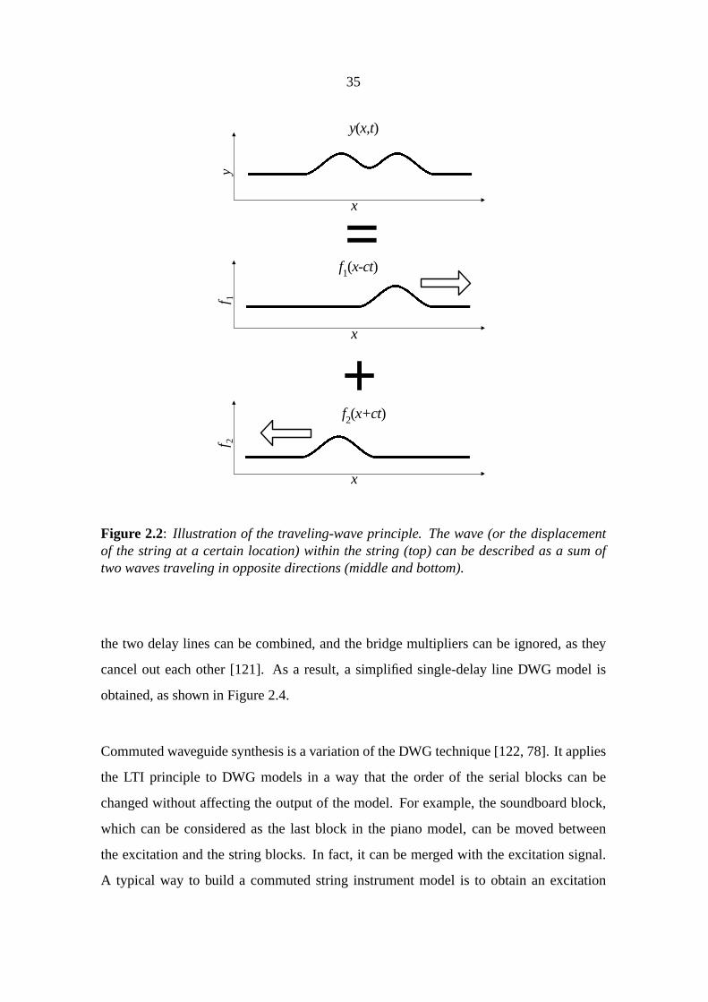
2.2 Illustration of the traveling-wave principle. The wave (or the displace-

ment of the string at a certain location) within the string (top) can be

described as a sum of two waves traveling in opposite directions (middle

and bottom).. . . . . . . . . . . . . . . . . . . . . . . . . . . . . . . . 35

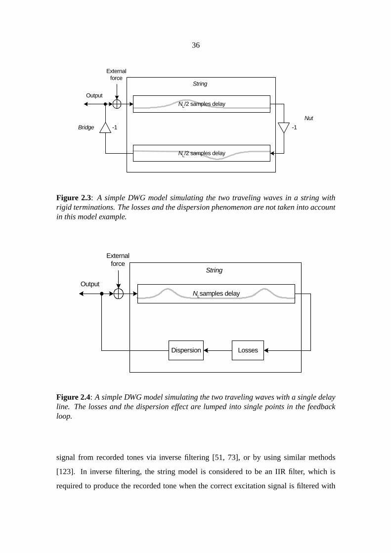
2.3 A simple DWG model simulating the two traveling waves in a string with

rigid terminations. The losses and the dispersion phenomenon are not

taken into account in this model example.. . . . . . . . . . . . . . . . 36

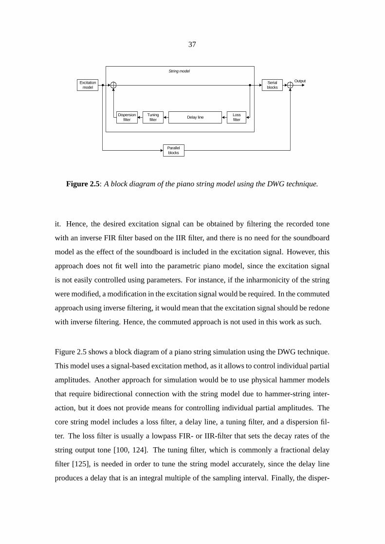
2.4 A simple DWG model simulating the two traveling waves with a single

delay line. The losses and the dispersion effect are lumped into single

points in the feedback loop.. . . . . . . . . . . . . . . . . . . . . . . . 36

2.5 A block diagram of the piano string model using the DWG technique.. . 37

3.1 Block diagram of the basic DWG piano string model considered in this

work. . . . . . . . . . . . . . . . . . . . . . . . . . . . . . . . . . . . 39

3.2 Block diagram of the excitation model.. . . . . . . . . . . . . . . . . . 41

3.3 An illustration of how the dispersion phenomenon affects the time-frequency

properties of the harmonics. (a) The waveform and (b) the spectrogram

of a harmonic tone (f0 = 100Hz, B = 0). (c) The waveform and (d) the

spectrogram of an inharmonic tone (f0 = 100Hz, B = 0.0001). . . . . 43

3.4 Examples of how the PFD curve behaves in three situations: too low aB

estimate value (left), an accurateB estimate value (middle), and too high

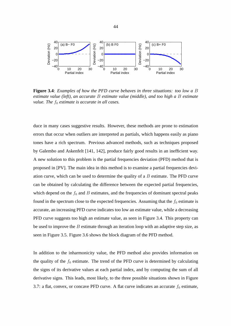
a B estimate value. Thef0 estimate is accurate in all cases.. . . . . . 44

22

3.5 An example of how the PFD method progresses in the iteration pro-

cess using a synthetic input signal (f0=38.9 Hz,B=0.0003). This figure

shows the PFD curve (deviation as a function of partial index) in itera-

tion rounds 1–20. The deviation is large in the beginning, but is reduced

significantly after several iteration rounds. The last deviation curves are

very smooth indicating that the modifiedB estimate value (B estimate at

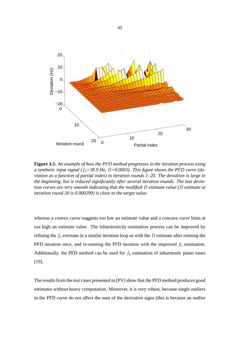
iteration round 20 is 0.000299) is close to the target value.. . . . . . . 45

3.6 Block diagram of the PFD method.. . . . . . . . . . . . . . . . . . . . 46

3.7 Examples of how the PFD curve behaves in three situations: too high a

B estimate and too low anf0 estimate (left), accuratef0 andB estimates

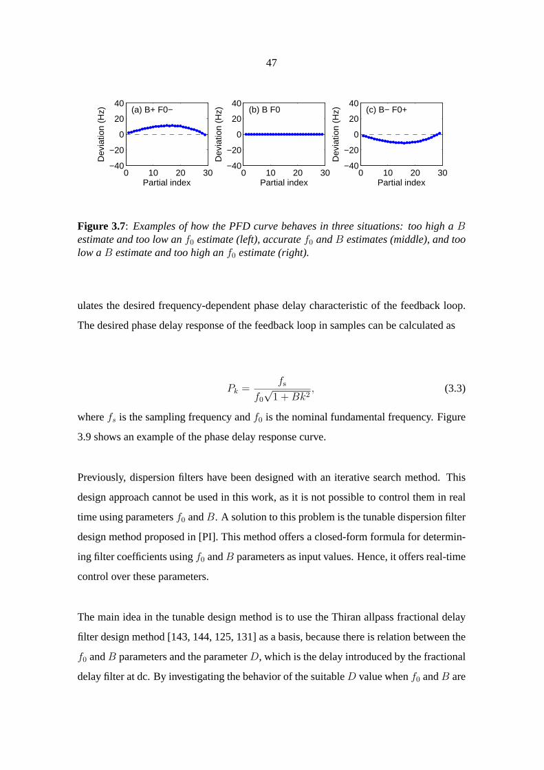
(middle), and too low aB estimate and too high anf0 estimate (right).. 47

3.8 An example of estimated inharmonicity values for key indices 1–50 using

the PFD method. Manually estimatedf0 values were used in the esti-

mation. Steinway grand piano samples were obtained from University of

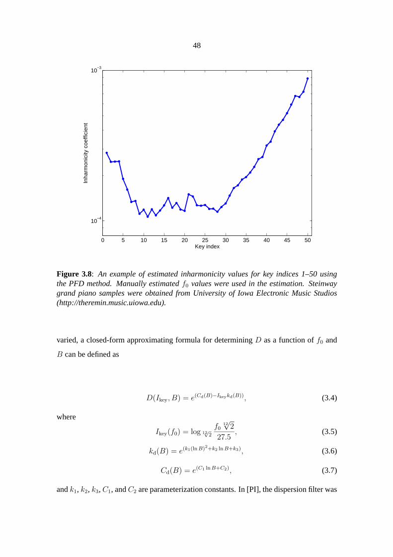
Iowa Electronic Music Studios (http://theremin.music.uiowa.edu).. . . 48

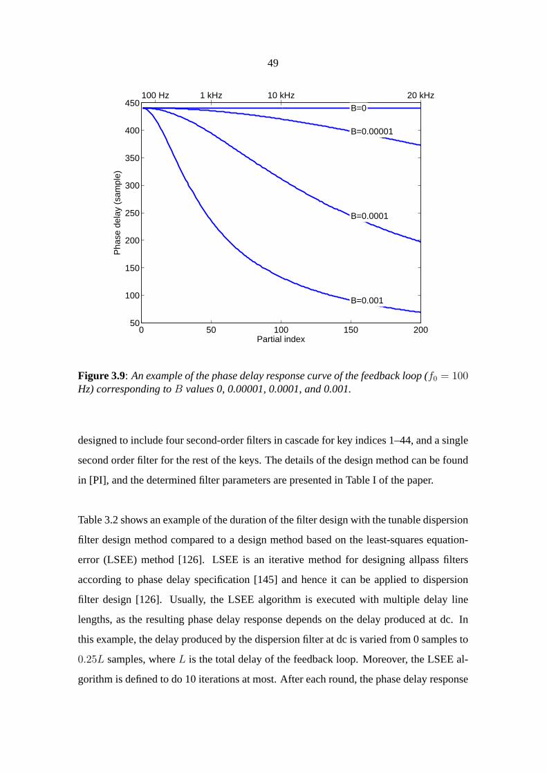
3.9 An example of the phase delay response curve of the feedback loop (f0 =

100 Hz) corresponding toB values 0, 0.00001, 0.0001, and 0.001.. . . 49

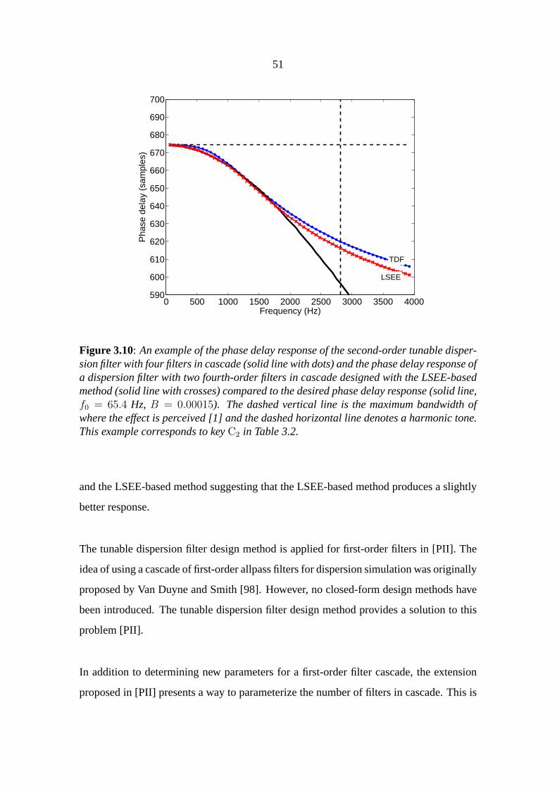
3.10 An example of the phase delay response of the second-order tunable dis-

persion filter with four filters in cascade (solid line with dots) and the

phase delay response of a dispersion filter with two fourth-order filters in

cascade designed with the LSEE-based method (solid line with crosses)

compared to the desired phase delay response (solid line,f0 = 65.4 Hz,

B = 0.00015). The dashed vertical line is the maximum bandwidth of

where the effect is perceived [1] and the dashed horizontal line denotes a

harmonic tone. This example corresponds to keyC2 in Table 3.2. . . . . 51

23

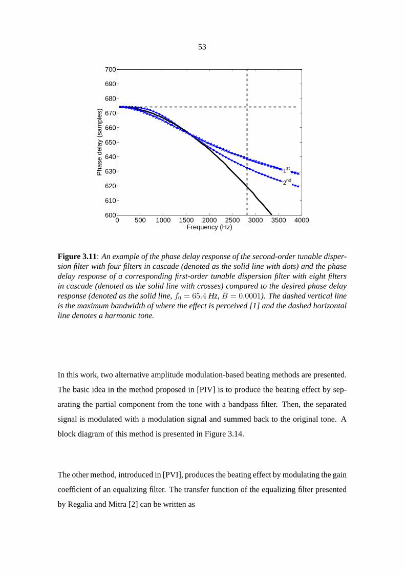
3.11 An example of the phase delay response of the second-order tunable dis-

persion filter with four filters in cascade (denoted as the solid line with

dots) and the phase delay response of a corresponding first-order tunable

dispersion filter with eight filters in cascade (denoted as the solid line

with crosses) compared to the desired phase delay response (denoted as

the solid line,f0 = 65.4 Hz,B = 0.0001). The dashed vertical line is the

maximum bandwidth of where the effect is perceived [1] and the dashed

horizontal line denotes a harmonic tone.. . . . . . . . . . . . . . . . . 53

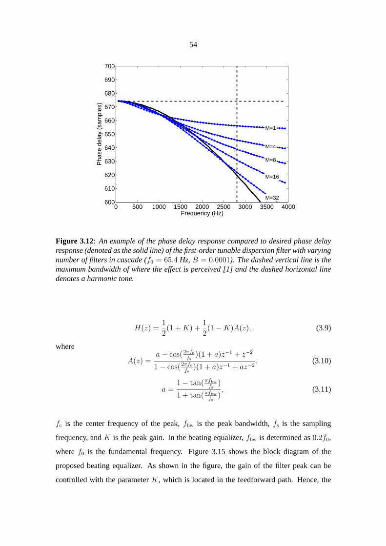
3.12 An example of the phase delay response compared to desired phase de-

lay response (denoted as the solid line) of the first-order tunable dis-

persion filter with varying number of filters in cascade (f0 = 65.4 Hz,

B = 0.0001). The dashed vertical line is the maximum bandwidth of

where the effect is perceived [1] and the dashed horizontal line denotes a

harmonic tone. . . . . . . . . . . . . . . . . . . . . . . . . . . . . . . 54

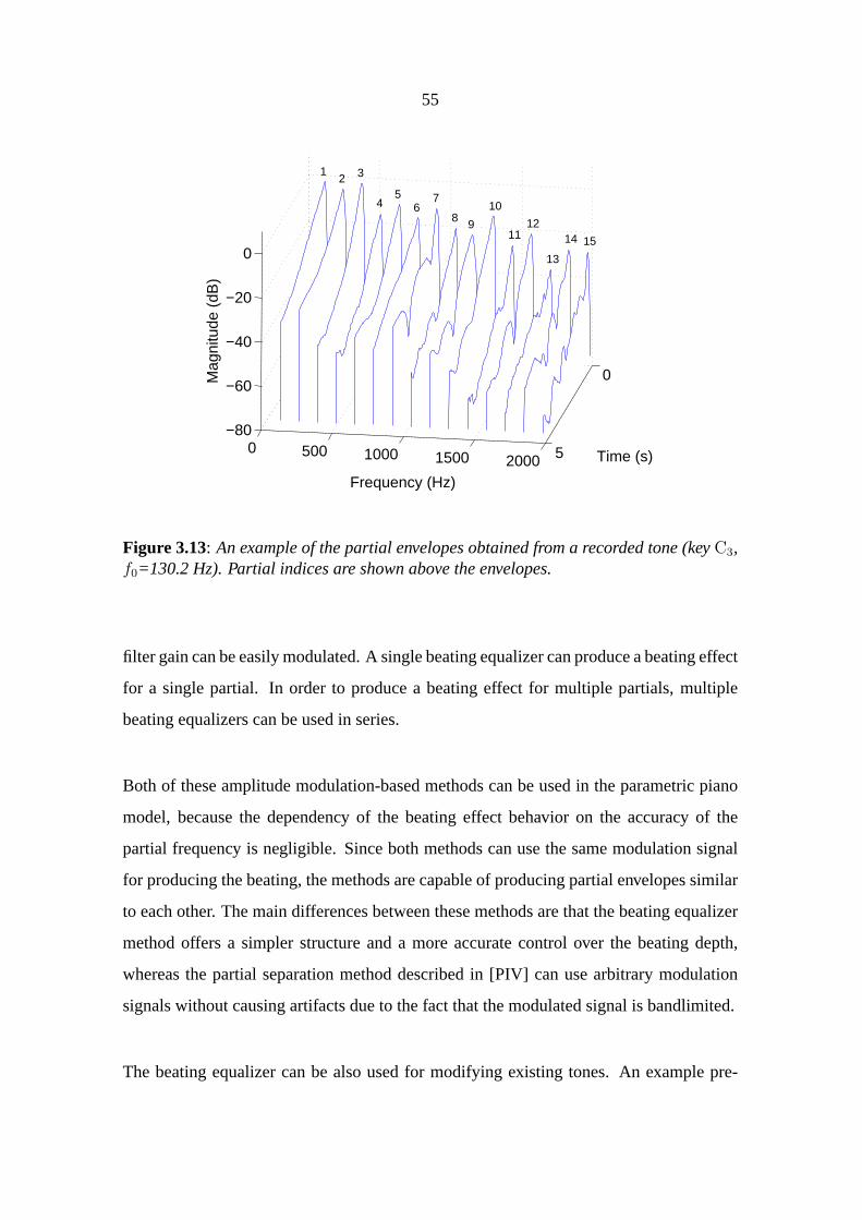
3.13 An example of the partial envelopes obtained from a recorded tone (key

C3, f0=130.2 Hz). Partial indices are shown above the envelopes.. . . 55

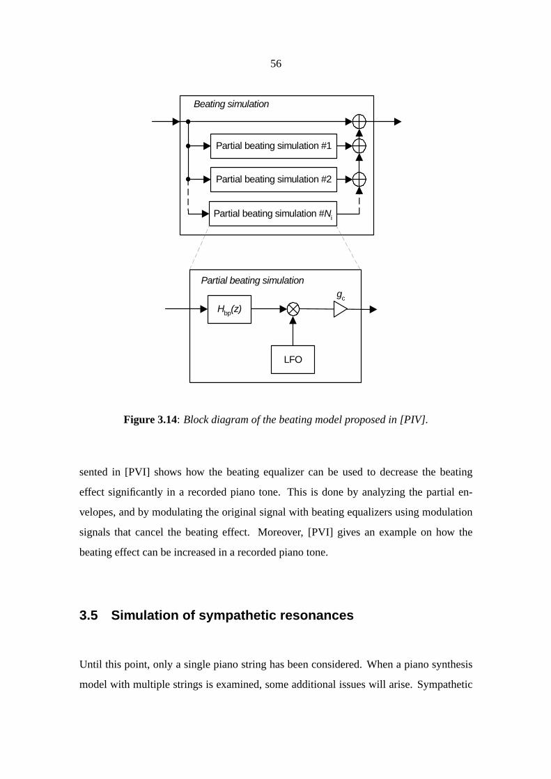
3.14 Block diagram of the beating model proposed in [PIV].. . . . . . . . . 56

3.15 Block diagram of the beating equalizer, which uses the equalizing filter

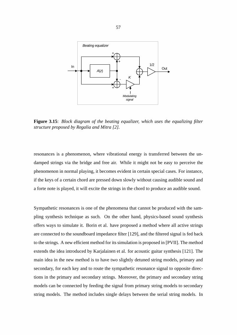
structure proposed by Regalia and Mitra [2].. . . . . . . . . . . . . . 57

3.16 Block diagram of the sympathetic resonances simulation method.Si,1

denotes the primary string model of keyi, andSi,2 denotes the secondary

string model. . . . . . . . . . . . . . . . . . . . . . . . . . . . . . . . 58

3.17 Block diagram of the sympathetic resonances simulation method of a sin-

gle key. . . . . . . . . . . . . . . . . . . . . . . . . . . . . . . . . . . 59

3.18 Examples of string model output envelopes of keysC2, E4, andG4, when

the string models are connected with the proposed sympathetic resonance

simulation method. In this case, a loud staccato note played on keyC2

causing energy flow to the strings corresponding to the other keys, which

is seen in the envelopes as an additional string excitation at around one

second. The envelopes are scaled in order to emphasize the phenomenon.60

24

3.19 Screenshot of the piano string model implemented in PWGL software

(adapted from Figure 13 of [PVII]). The excitation model is denoted

as pno-excitation, the combined delay line and loss filter block as pno-

multi-ripple, the dispersion filter as pno-dispersion, the tuning filter as

pno-tuningfilter, and the combined beating and knocking tone block as

hammer-beating. . . . . . . . . . . . . . . . . . . . . . . . . . . . . . 62

25

List of Tables

3.1 Piano model components and the requirements for each component to

enable the real-time control of parametersf0 andB. . . . . . . . . . . 40

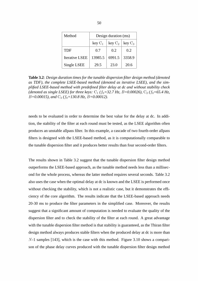
3.2 Design duration times for the tunable dispersion filter design method (de-

noted as TDF), the complete LSEE-based method (denoted as iterative

LSEE), and the simplified LSEE-based method with predefined filter de-

lay at dc and without stability check (denoted as single LSEE) for three

keys:C1 (f0=32.7 Hz,B=0.00026),C2 (f0=65.4 Hz,B=0.00015), and

C3 (f0=130.8 Hz,B=0.00012).. . . . . . . . . . . . . . . . . . . . . . 50

26

27

1 Introduction

This thesis discusses sound synthesis of the piano using physics-based methods. Sound

synthesis can be categorized under the music technology research field. Moreover, in

order to develop sound synthesis methods, sound analysis, which belongs to the group

of musical acoustics, is done along with sound synthesis. The term physics-based sound

synthesis, or physically inspired sound synthesis, can be used to describe a synthesis

method, which uses physical models and signal processing methods for simulating phe-

nomena occurring in the sound [3, 4, 5].

The two most common physical modeling techniques used in sound synthesis are the

digital waveguide technique (DWG) [6, 7] and the finite difference method (FD) [8, 9].

The DWG technique can be used to develop simplified and efficient physical models,

whereas the FD method produces models that are directly derived from real physical

parameters at the cost of increased computational load compared to the DWG.

In this work, a piano synthesis model is developed using the DWG technique. The main

goal is to develop a parametric model that can be controlled in real-time by computing

model coefficients on the fly. In addition, the model is required to be efficient without

compromising the perceived sound quality. Another aspect of this work is to pay special

attention to the inharmonicity phenomenon, which is a characteristic of the piano.

1.1 Scope of the research

The primary goal for this thesis is to develop methods that enable the implementation of

a parametric, real-time piano synthesizer allowing dynamic online control over the model

parameters. Elements that are considered include the excitation model, dispersion fil-

ter, and beating simulation. Special attention is paid to the fundamental frequency and

28

inharmonicity coefficient parameters that affect most of the components in the model.

Moreover, a method for simulating sympathetic resonances in a piano synthesis model

is considered. Finally, a real-time implementation based on the developed methods is

created. Another goal in this work is to develop methods that simulate the desired phe-

nomena in an efficient way suitable for real-time implementation. An important aspect

that can be used in optimizing the methods is the human auditory system and its prop-

erties. In other words, it is better to direct the memory and computational resources to

parts that are perceptually important. Moreover, the model can be simplified and stripped

down in places that do not affect the perceived sound. In addition to the perceptual infor-

mation [10, 11, 12, 13, 14, 15], also signal processing techniques are used for improving

simulation methods.

1.2 Main results

This thesis work has produced the following results:

• The first closed-form method for designing dispersion filters using first- or second-

order allpass filters.

• A new parametric excitation model, which provides a direct control of the simu-

lation parameters, such as the fundamental frequency and the inharmonicity coef-

ficient value.

• A novel inharmonicity estimation algorithm that is efficient and robust.

• Two new beating simulation techniques that offer direct control of the beating

parameters. One of these techniques can be used for both synthesis and analysis

purposes, as it can be used to modify partial envelopes of arbitrary tones.

• A new method for simulating sympathetic resonances in a piano synthesis model.

29

• A real-time piano synthesizer developed in co-operation with the Sibelius Academy.

The main area where these results can be applied is physics-based piano synthesis. Due

to the highly parametric methods, the model can be scaled down to be used in restricted

environments, such as mobile phones and game platforms.Moreover, the real-time para-

metric control over the fundamental frequency and inharmonicity coefficient parameters

offers a piano model, where these parameters can be tuned in a similar fashion as the fun-

damental frequencies are tuned in a real grand piano.Other application fields for piano

synthesis are signal analysis, such as transcription of piano music [16, 17, 18], and analy-

sis of the perception [10, 11, 12, 13, 14], where it can be used for producing realistic test

tones. Additionally, the inharmonicity estimation algorithm can be used for signal anal-

ysis, namely for estimating fundamental frequencies [19] and inharmonicity coefficient

values from recorded string instrument tones.

30

2 Background

2.1 Acoustics of the piano

The piano is one of the most popular instruments in western music. It is an essential

instrument in many musical styles ranging from jazz to classical and pop. The modern

piano has evolved from the 18th century predecessor called "gravicembalo col piano et

forte", which can be considered as a modified harpsichord [20]. Today, there are two types

of pianos available: grand pianos and upright pianos. Grand pianos, where the strings are

laid horizontally, are popular in the professional context due to excellent sound quality,

whereas upright pianos with vertical strings are suitable for homes as they are smaller and

cheaper to purchase. Another advantage that the grand piano has over the upright piano

is that it enables fast repetitions on the same note. This work concentrates on the grand

piano.

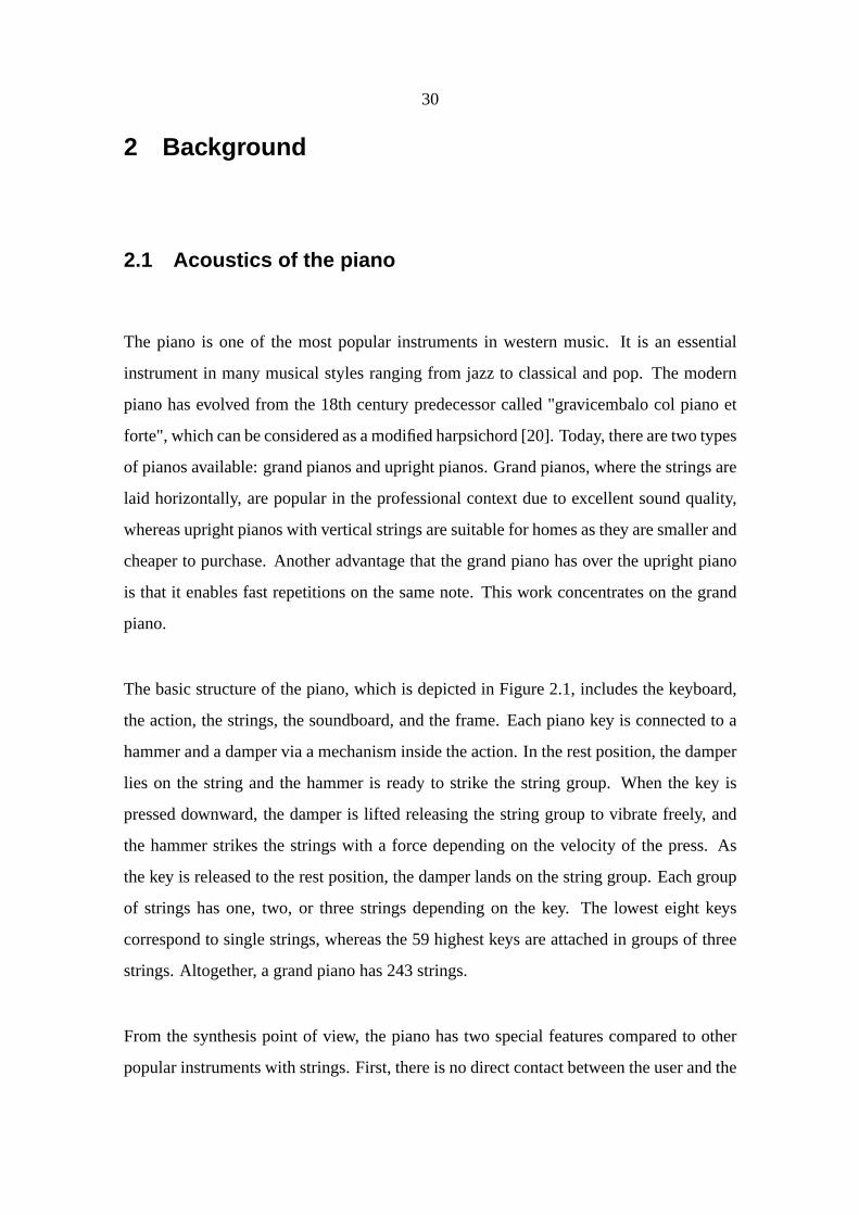
The basic structure of the piano, which is depicted in Figure 2.1, includes the keyboard,

the action, the strings, the soundboard, and the frame. Each piano key is connected to a

hammer and a damper via a mechanism inside the action. In the rest position, the damper

lies on the string and the hammer is ready to strike the string group. When the key is

pressed downward, the damper is lifted releasing the string group to vibrate freely, and

the hammer strikes the strings with a force depending on the velocity of the press. As

the key is released to the rest position, the damper lands on the string group. Each group

of strings has one, two, or three strings depending on the key. The lowest eight keys

correspond to single strings, whereas the 59 highest keys are attached in groups of three

strings. Altogether, a grand piano has 243 strings.

From the synthesis point of view, the piano has two special features compared to other

popular instruments with strings.First, there is no direct contact between the user and the

31

Soundboard BridgeString

Hammer

Damper

Pin block

Key

Action

Figure 2.1: Structure of the piano.

strings, for example as in the guitar, making the excitation process from the sound synthe-

sis point of view somewhat easier.On the other hand, the piano has a very complex struc-

ture with over two hundred strings, which is very challenging for the synthesis. The most

significant phenomena from the piano tone point of view are dispersion, two-stage de-

cay, beating, frequency-dependent decaying, and phantom partials. The two-stage decay

means that in the beginning the piano tone decays rapidly but after some tenths of a sec-

ond the decaying slows down. This is explained by the shift in the dominating vibration

from vertical to horizontal [21]. Moreover, the phantom partials effect is a phenomenon

occurring in the fortissimo piano tones due to longitudinal modes [22, 23, 24].The gen-

eral acoustics of the piano is well described, for example in [25, 26, 27, 28], while details

on the hammer-string interaction are available in [29, 30, 31, 32, 33, 34, 35, 36, 37, 38],

32

and the acoustical phenomena related to piano strings are presented in [39, 40, 41, 42].

Additionally, the mechanics of the piano soundboard and its effect on the piano acoustics

can be found in [43, 44, 45, 46]. Also, characteristics of a piano tone are described in

[47, 48, 49].

2.2 Physics-based sound synthesis of the piano

2.2.1 Physics-based methods in sound synthesis

In physics-based sound synthesis [3, 50, 4, 5, 51], the goal is to simulate the sound

source instead of just the sound itself. Currently, there are six synthesis methods that are

considered physical modeling techniques: finite-difference (FD), mass-spring networks,

wave digital filters (WDF), modal synthesis, source-filter modeling, and digital waveg-

uide (DWG) [52, 53]. In practice, there are two main approaches in applying physical

modeling techniques. The first approach prefers to use strict physical modeling, while

the other concentrates on developing computationally efficient physics-based methods.

This is done by using physical modeling as the basis for the synthesis and by applying

signal processing methods to improve computational efficiency. This work uses the latter

approach.

One of the great advantages of the physics-based approach is its support for parametric

control of the model. While the sampling synthesis technique can be used to produce

high-quality piano tones, it does not offer the same kind of flexibility as physics-based

models. For instance, in order to change the pitch of a string, the sampling technique

needs additional signal processing methods to perform the change.On the other hand,

the fundamental frequency is one of the main internal parameters in physics-based string

models and, hence, it can be easily modified offline. Online control over parameters

introduces challenges that are dealt in this work.

33

FD modeling is based on the numerical solution of partial differential equations [8, 9, 54].

It can be used to develop very accurate physical models. Moreover, it maps physical

parameters directly to the equations. The major disadvantage in sound synthesis is its

computational inefficiency [55]. Another inefficient physical modeling technique is mass-

spring networks, which uses finite masses, springs, and dampers to define a physical

system [56]. The WDF method has been also used for sound synthesis. It was originally

developed for representing electrical analog circuits in the digital domain with equivalent

elements [57], but later it has been applied to other domains, including the acoustical

domain enabling sound synthesis [58]. In modal synthesis, the goal is to simulate the

modes of vibrations [59, 60].Recently, modal synthesis principles have been applied to

sound synthesis by using the functional transformation method [61, 62].The source-filter

technique that uses time-variant filters is also considered as physical modeling technique

[63, 64]. The DWG technique is presented in Section 2.2.2.

The DWG technique and the FD method are the most common physical modeling tech-

niques used for the synthesis of the piano. Chaigne and Askenfelt have developed a piano

synthesis model using the FD technique [65, 66]. Another more recent FD piano simu-

lation has been presented by Giordano and Jiang [67]. Moreover, Bank and Sujbert has

used the FD method for simulating longitudinal modes [68]. Furthermore, some work

has been done using the source-filter-based approach for piano synthesis [69, 70]. Other

techniques have been used as well for describing single subsystems of a piano synthesis

model. For instance, Van Duyne and Smith have proposed a hammer model using the

WDF technique [71].

2.2.2 Piano synthesis using digital waveguides

The DWG technique, which can be considered as an extension of the Karplus-Strong

algorithm [72], is a popular physical modeling technique [6, 7].It is well suited, for

example, for modeling string and wind instruments. It has been applied, for example,

34

to synthesize of the acoustic guitar [73, 74, 75], the bass guitar [76], traditional string

instruments [77, 78, 79, 80, 81, 82, 83, 84], woodwinds [85, 86, 87], brass instruments

[88, 89], the violin [90, 91, 92, 93], the harpsichord [94], and the clavichord [95].

The DWG technique is perhaps the most common physical modeling technique in physics-

based piano synthesis. The first DWG piano model was developed by Garnett [96].

Since then, work in DWG piano synthesis has been done, e.g., by Van Duyne and Smith

[97, 98, 99, 100, 101] and Aramaki et al. [102].Moreover, Bensa and his colleagues have

conducted research on piano string modeling [103, 104, 105, 106], hammer-string inter-

action [107, 108, 109], and phantom partials [110]. Also, Bank and his co-authors have

worked on the nonlinearities in DWG piano modeling [111, 112, 113], on the simulation

of the beating effect [114, 115, 116], on loss-filter design [117], and on the modeling

of longitudinal modes [24, 118, 68]. Additionally, excellent reviews on the DWG piano

synthesis are available in [119, 120].

The basis of the DWG technique is the discretization of the traveling-wave equation

y = f1(x− ct) + f2(x + ct), (2.1)

wheref1 andf2 describe two waves traveling in opposite directions,x is the location on

the string,c is the speed of sound,t is time, andy is the displacement of the string from

its rest position. This is further illustrated in Figure 2.2. Figure 2.3 shows a DWG model

simulating an ideal string with rigid terminations [7]. In other words, each traveling wave

f1 andf2 corresponds to an equal-length delay line.The external force in Figure 2.3 refers

to the force that excites the string to vibrate, namely, in this case, the hammer strike.

When the losses and the dispersion occurring in a real string are taken into account, the

model includesL dispersion blocks and loss blocks equally distributed along the delay

lines, whereNL is the total length of the delay lines in samples.However, if the output of

the string system is taken at a single point, these blocks can be combined using linear and

time-invariant (LTI) principles into a single dispersion block and a loss block. Moreover,

35

+

=

y(x,t)

f1(x-ct)

f2(x+ct)

xy

x

f 1

x

f 2

Figure 2.2: Illustration of the traveling-wave principle. The wave (or the displacementof the string at a certain location) within the string (top) can be described as a sum oftwo waves traveling in opposite directions (middle and bottom).

the two delay lines can be combined, and the bridge multipliers can be ignored, as they

cancel out each other [121]. As a result, a simplified single-delay line DWG model is

obtained, as shown in Figure 2.4.

Commuted waveguide synthesis is a variation of the DWG technique [122, 78]. It applies

the LTI principle to DWG models in a way that the order of the serial blocks can be

changed without affecting the output of the model.For example, the soundboard block,

which can be considered as the last block in the piano model, can be moved between

the excitation and the string blocks. In fact, it can be merged with the excitation signal.

A typical way to build a commuted string instrument model is to obtain an excitation

36

String

BridgeNut

Externalforce

-1 -1

NL/2 samples delay

NL/2 samples delayOutput

Figure 2.3: A simple DWG model simulating the two traveling waves in a string withrigid terminations. The losses and the dispersion phenomenon are not taken into accountin this model example.

String

Externalforce

NLsamples delay

LossesDispersion

Output

Figure 2.4: A simple DWG model simulating the two traveling waves with a single delayline. The losses and the dispersion effect are lumped into single points in the feedbackloop.

signal from recorded tones via inverse filtering [51, 73], or by using similar methods

[123]. In inverse filtering, the string model is considered to be an IIR filter, which is

required to produce the recorded tone when the correct excitation signal is filtered with

37

String model

Delay line Lossfilter

Dispersionfilter

Output

Tuningfilter

Excitationmodel

Parallelblocks

Serialblocks

Figure 2.5: A block diagram of the piano string model using the DWG technique.

it. Hence, the desired excitation signal can be obtained by filtering the recorded tone

with an inverse FIR filter based on the IIR filter, and there is no need for the soundboard

model as the effect of the soundboard is included in the excitation signal.However, this

approach does not fit well into the parametric piano model, since the excitation signal

is not easily controlled using parameters. For instance, if the inharmonicity of the string

were modified, a modification in the excitation signal would be required. In the commuted

approach using inverse filtering, it would mean that the excitation signal should be redone

with inverse filtering. Hence, the commuted approach is not used in this work as such.

Figure 2.5 shows a block diagram of a piano string simulation using the DWG technique.

This model uses a signal-based excitation method, as it allows to control individual partial

amplitudes. Another approach for simulation would be to use physical hammer models

that require bidirectional connection with the string model due to hammer-string inter-

action, but it does not provide means for controlling individual partial amplitudes.The

core string model includes a loss filter, a delay line, a tuning filter, and a dispersion fil-

ter. The loss filter is usually a lowpass FIR- or IIR-filter that sets the decay rates of the

string output tone [100, 124]. The tuning filter, which is commonly a fractional delay

filter [125], is needed in order to tune the string model accurately, since the delay line

produces a delay that is an integral multiple of the sampling interval. Finally, the disper-

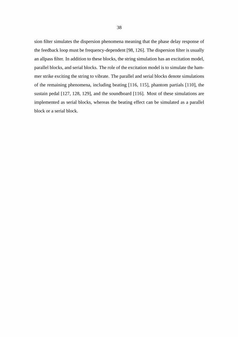
38

sion filter simulates the dispersion phenomena meaning that the phase delay response of

the feedback loop must be frequency-dependent [98, 126]. The dispersion filter is usually

an allpass filter. In addition to these blocks, the string simulation has an excitation model,

parallel blocks, and serial blocks. The role of the excitation model is to simulate the ham-

mer strike exciting the string to vibrate. The parallel and serial blocks denote simulations

of the remaining phenomena, including beating [116, 115], phantom partials [110], the

sustain pedal [127, 128, 129], and the soundboard [116]. Most of these simulations are

implemented as serial blocks, whereas the beating effect can be simulated as a parallel

block or a serial block.

39

String model

Delay line Lossfilter

Dispersionfilter

Output

Tuningfilter

Excitationmodel

Beatingsimulation

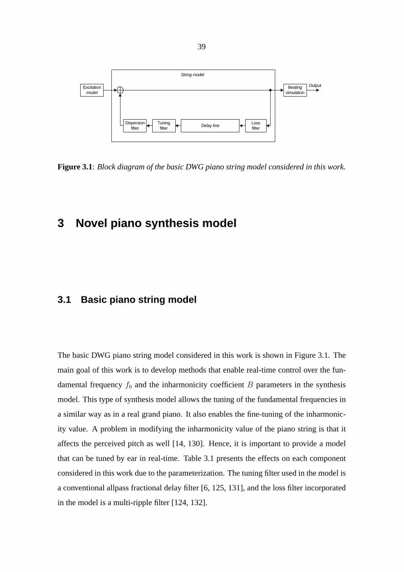
Figure 3.1: Block diagram of the basic DWG piano string model considered in this work.

3 Novel piano synthesis model

3.1 Basic piano string model

The basic DWG piano string model considered in this work is shown in Figure 3.1. The

main goal of this work is to develop methods that enable real-time control over the fun-

damental frequencyf0 and the inharmonicity coefficientB parameters in the synthesis

model. This type of synthesis model allows the tuning of the fundamental frequencies in

a similar way as in a real grand piano. It also enables the fine-tuning of the inharmonic-

ity value. A problem in modifying the inharmonicity value of the piano string is that it

affects the perceived pitch as well [14, 130]. Hence, it is important to provide a model

that can be tuned by ear in real-time. Table 3.1 presents the effects on each component

considered in this work due to the parameterization. The tuning filter used in the model is

a conventional allpass fractional delay filter [6, 125, 131], and the loss filter incorporated

in the model is a multi-ripple filter [124, 132].

40

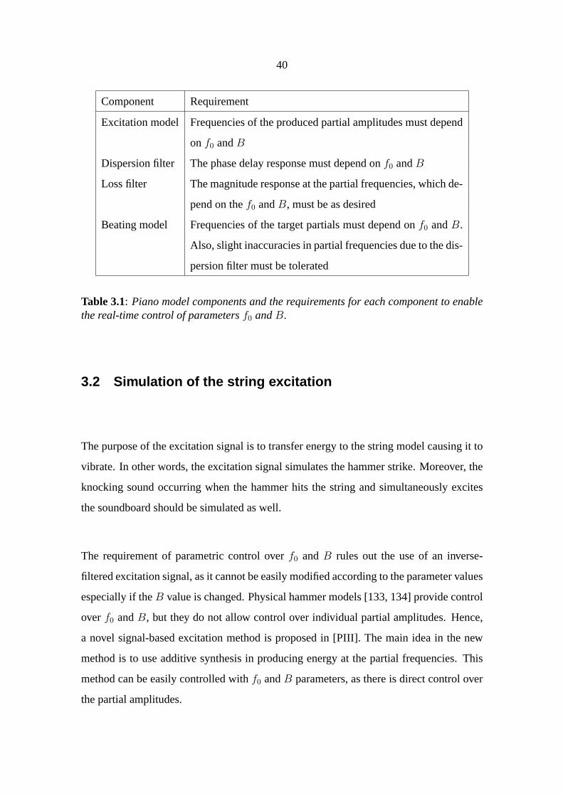
Component Requirement

Excitation model Frequencies of the produced partial amplitudes must depend

onf0 andB

Dispersion filter The phase delay response must depend onf0 andB

Loss filter The magnitude response at the partial frequencies, which de-

pend on thef0 andB, must be as desired

Beating model Frequencies of the target partials must depend onf0 andB.

Also, slight inaccuracies in partial frequencies due to the dis-

persion filter must be tolerated

Table 3.1: Piano model components and the requirements for each component to enablethe real-time control of parametersf0 andB.

3.2 Simulation of the string excitation

The purpose of the excitation signal is to transfer energy to the string model causing it to

vibrate. In other words, the excitation signal simulates the hammer strike.Moreover, the

knocking sound occurring when the hammer hits the string and simultaneously excites

the soundboard should be simulated as well.

The requirement of parametric control overf0 andB rules out the use of an inverse-

filtered excitation signal, as it cannot be easily modified according to the parameter values

especially if theB value is changed.Physical hammer models [133, 134] provide control

overf0 andB, but they do not allow control over individual partial amplitudes. Hence,

a novel signal-based excitation method is proposed in [PIII].The main idea in the new

method is to use additive synthesis in producing energy at the partial frequencies. This

method can be easily controlled withf0 andB parameters, as there is direct control over

the partial amplitudes.

41

Additivesynthesis

Noise

EQ

Shaping window

Keynumber

Note onevent

Out

LP

Key pressvelocity

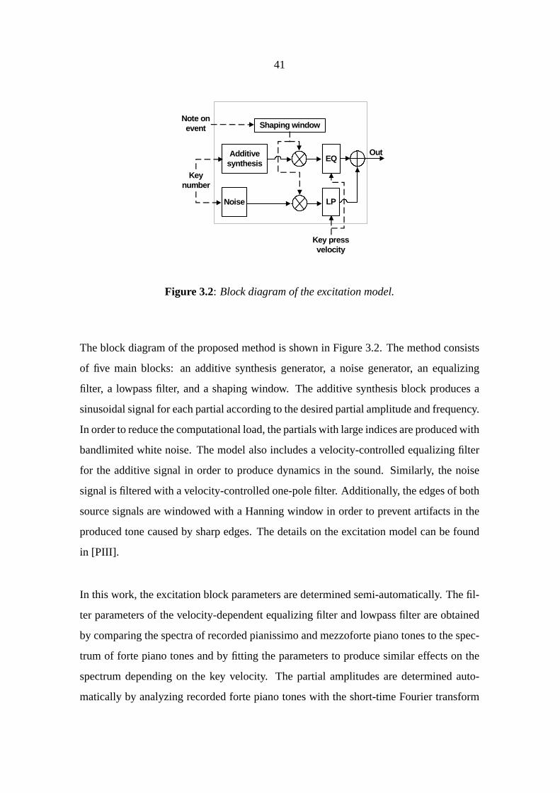
Figure 3.2: Block diagram of the excitation model.

The block diagram of the proposed method is shown in Figure 3.2.The method consists

of five main blocks: an additive synthesis generator, a noise generator, an equalizing

filter, a lowpass filter, and a shaping window. The additive synthesis block produces a

sinusoidal signal for each partial according to the desired partial amplitude and frequency.

In order to reduce the computational load, the partials with large indices are produced with

bandlimited white noise. The model also includes a velocity-controlled equalizing filter

for the additive signal in order to produce dynamics in the sound. Similarly, the noise

signal is filtered with a velocity-controlled one-pole filter. Additionally, the edges of both

source signals are windowed with a Hanning window in order to prevent artifacts in the

produced tone caused by sharp edges. The details on the excitation model can be found

in [PIII].

In this work, the excitation block parameters are determined semi-automatically. The fil-

ter parameters of the velocity-dependent equalizing filter and lowpass filter are obtained

by comparing the spectra of recorded pianissimo and mezzoforte piano tones to the spec-

trum of forte piano tones and by fitting the parameters to produce similar effects on the

spectrum depending on the key velocity. The partial amplitudes are determined auto-

matically by analyzing recorded forte piano tones with the short-time Fourier transform

42

(STFT). Then, the maximum value of each partial envelope is set to be the partial am-

plitude. Finally, the extracted partial amplitudes are evaluated and, if needed, modified

manually.

Piano sound can be separated into a harmonic component (caused by the excited string)

and a broadband component (the knocking sound) [128, 47, 135]. The knocking sound

is not audible in the bass range, but in the treble range it plays a significant part in the

perceived piano sound [136]. Hence, a knocking sound simulating the sound caused

by the hammer striking the strings is required in addition to the excitation signal. The

knocking sound can be included in the excitation signal, or it can be summed into the

signal produced by the string model. The latter option is used in this work, since it does

not require any compensation in the partial amplitudes due to the spectral components

in the knocking sound. The sound can be produced by using the modal synthesis-based

approach presented in [PVII]. An alternative approach is to use processed recorded tones

such as an inverse-filtered piano tone.

3.3 Simulation of dispersion

3.3.1 Analysis of the dispersion phenomenon

Piano strings are known to be dispersive due to the stiffness of the string material. Dis-

persion means that these properties resist the free flexible movement of the string.It is

suggested that the soundboard impedance contributes to the inharmonicity as well [137].

As a result, high frequency components in the tone travel faster than low frequency com-

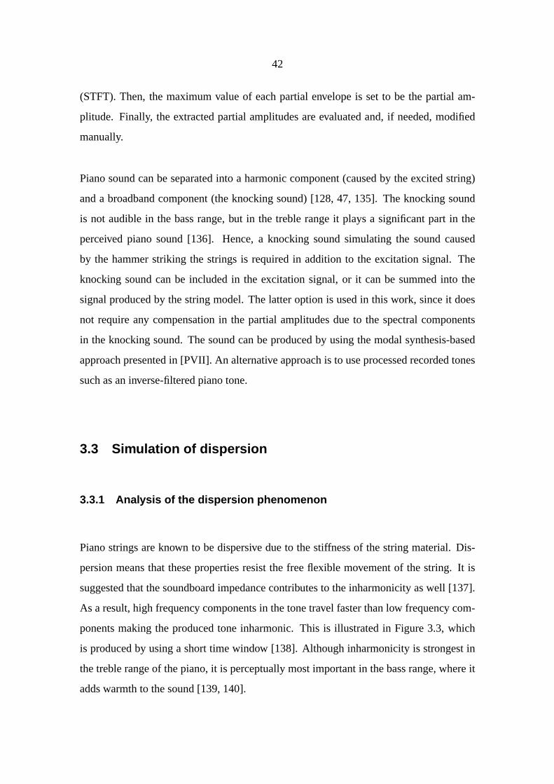
ponents making the produced tone inharmonic. This is illustrated in Figure 3.3, which

is produced by using a short time window [138]. Although inharmonicity is strongest in

the treble range of the piano, it is perceptually most important in the bass range, where it

adds warmth to the sound [139, 140].

43

0 0.005 0.01 0.015 0.02 0.025 0.03 0.035 0.04

−1

−0.5

0

0.5

1

Time (ms)

Am

plitu

de

(a)Time (ms)

Fre

quen

cy (

Hz)

0 0.005 0.01 0.015 0.02 0.025 0.03 0.035 0.040

1000

2000

3000

4000

(b)

0 0.005 0.01 0.015 0.02 0.025 0.03 0.035 0.04

−0.5

0

0.5

1

Time (ms)

Am

plitu

de

(c)Time (ms)

Fre

quen

cy (

Hz)

0 0.005 0.01 0.015 0.02 0.025 0.03 0.035 0.040

1000

2000

3000

4000

(d)

Figure 3.3: An illustration of how the dispersion phenomenon affects the time-frequencyproperties of the harmonics. (a) The waveform and (b) the spectrogram of a harmonictone (f0 = 100Hz, B = 0). (c) The waveform and (d) the spectrogram of an inharmonictone (f0 = 100Hz, B = 0.0001).

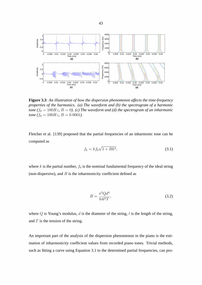
Fletcher et al. [139] proposed that the partial frequencies of an inharmonic tone can be

computed as

fk = kf0

√1 + Bk2, (3.1)

wherek is the partial number,f0 is the nominal fundamental frequency of the ideal string

(non-dispersive), andB is the inharmonicity coefficient defined as

B =π3Qd4

64l2T, (3.2)

whereQ is Young’s modulus,d is the diameter of the string,l is the length of the string,

andT is the tension of the string.

An important part of the analysis of the dispersion phenomenon in the piano is the esti-

mation of inharmonicity coefficient values from recorded piano tones.Trivial methods,

such as fitting a curve using Equation 3.1 to the determined partial frequencies, can pro-

44

0 10 20 30−40

−20

0

20

40

Partial index

Dev

iatio

n (H

z) (c) B+ F0

0 10 20 30−40

−20

0

20

40

Partial index

Dev

iatio

n (H

z) (a) B− F0

0 10 20 30−40

−20

0

20

40

Partial index

Dev

iatio

n (H

z) (b) B F0

Figure 3.4: Examples of how the PFD curve behaves in three situations: too low aBestimate value (left), an accurateB estimate value (middle), and too high aB estimatevalue. Thef0 estimate is accurate in all cases.

duce in many cases suggestive results. However, these methods are prone to estimation

errors that occur when outliers are interpreted as partials, which happens easily as piano

tones have a rich spectrum.Previous advanced methods, such as techniques proposed

by Galembo and Askenfelt [141, 142], produce fairly good results in an inefficient way.

A new solution to this problem is the partial frequencies deviation (PFD) method that is

proposed in [PV]. The main idea in this method is to examine a partial frequencies devi-

ation curve, which can be used to determine the quality of aB estimate.The PFD curve

can be obtained by calculating the difference between the expected partial frequencies,

which depend on thef0 andB estimates, and the frequencies of dominant spectral peaks

found in the spectrum close to the expected frequencies.Assuming that thef0 estimate is

accurate, an increasing PFD curve indicates too low an estimate value, while a decreasing

PFD curve suggests too high an estimate value, as seen in Figure 3.4. This property can

be used to improve theB estimate through an iteration loop with an adaptive step size, as

seen in Figure 3.5. Figure 3.6 shows the block diagram of the PFD method.

In addition to the inharmonicity value, the PFD method also provides information on

the quality of thef0 estimate.The trend of the PFD curve is determined by calculating

the signs of its derivative values at each partial index, and by computing the sum of all

derivative signs. This leads, most likely, to the three possible situations shown in Figure

3.7: a flat, convex, or concave PFD curve.A flat curve indicates an accuratef0 estimate,

45

0

10

20 010

2030

−20

−10

0

10

20

Partial indexIteration round

Dev

iatio

n (H

z)

Figure 3.5: An example of how the PFD method progresses in the iteration process usinga synthetic input signal (f0=38.9 Hz,B=0.0003). This figure shows the PFD curve (de-viation as a function of partial index) in iteration rounds 1–20. The deviation is large inthe beginning, but is reduced significantly after several iteration rounds. The last devia-tion curves are very smooth indicating that the modifiedB estimate value (B estimate atiteration round 20 is 0.000299) is close to the target value.

whereas a convex curve suggests too low an estimate value and a concave curve hints at

too high an estimate value. The inharmonicity estimation process can be improved by

refining thef0 estimate in a similar iteration loop as with theB estimate after running the

PFD iteration once, and re-running the PFD iteration with the improvedf0 estimation.

Additionally, the PFD method can be used forf0 estimation of inharmonic piano tones

[19].

The results from the test cases presented in [PV] show that the PFD method produces good

estimates without heavy computation.Moreover, it is very robust, because single outliers

in the PFD curve do not affect the sum of the derivative signs (this is because an outlier

46

Input signal B estimate

B estimation

Check stopconditions

Determinetrend of

deviation

FFT

Selectprominentspectralpeaks

Calculatepartial

frequencydeviation

Modify Bestimation

Bestimation

Bestimation

f0estimation

Spectral peakdata, initial B

estimate

Refined Bestimate

f0 estimation

Check stopconditions

Determinetrend of

deviation

Calculatepartial

frequencydeviation

Modify f0estimation

Spectral peakdata, initial f0

estimate

Refined f0estimate

Figure 3.6: Block diagram of the PFD method.

produces opposite derivative signs, which corresponds to zero in the sum). In addition,

the final PFD curve provides a good error indicator, as an almost flat curve suggests

successful estimation and a dispersed curve indicates inaccurate estimation. Figure 3.8

shows an example of inharmonicity values estimated from recorded piano tones using the

PFD method.

3.3.2 Dispersion filter design

The dispersion filter is an essential part of the DWG piano string model. As mentioned

previously, it is usually an allpass filter with a nonlinear phase delay response that sim-

47

0 10 20 30−40

−20

0

20

40

Partial index

Dev

iatio

n (H

z) (a) B+ F0−

0 10 20 30−40

−20

0

20

40

Partial index

Dev

iatio

n (H

z) (b) B F0

0 10 20 30−40

−20

0

20

40

Partial index

Dev

iatio

n (H

z) (c) B− F0+

Figure 3.7: Examples of how the PFD curve behaves in three situations: too high aBestimate and too low anf0 estimate (left), accuratef0 andB estimates (middle), and toolow aB estimate and too high anf0 estimate (right).

ulates the desired frequency-dependent phase delay characteristic of the feedback loop.

The desired phase delay response of the feedback loop in samples can be calculated as

Pk =fs

f0

√1 + Bk2

, (3.3)

wherefs is the sampling frequency andf0 is the nominal fundamental frequency. Figure

3.9 shows an example of the phase delay response curve.

Previously, dispersion filters have been designed with an iterative search method.This

design approach cannot be used in this work, as it is not possible to control them in real

time using parametersf0 andB. A solution to this problem is the tunable dispersion filter

design method proposed in [PI]. This method offers a closed-form formula for determin-

ing filter coefficients usingf0 andB parameters as input values. Hence, it offers real-time

control over these parameters.

The main idea in the tunable design method is to use the Thiran allpass fractional delay

filter design method [143, 144, 125, 131] as a basis, because there is relation between the

f0 andB parameters and the parameterD, which is the delay introduced by the fractional

delay filter at dc.By investigating the behavior of the suitableD value whenf0 andB are

48

0 5 10 15 20 25 30 35 40 45 50

10−4

10−3

Key index

Inha

rmon

icity

coe

ffici

ent

Figure 3.8: An example of estimated inharmonicity values for key indices 1–50 usingthe PFD method. Manually estimatedf0 values were used in the estimation. Steinwaygrand piano samples were obtained from University of Iowa Electronic Music Studios(http://theremin.music.uiowa.edu).

varied, a closed-form approximating formula for determiningD as a function off0 and

B can be defined as

D(Ikey, B) = e(Cd(B)−Ikeykd(B)), (3.4)

where

Ikey(f0) = log 12√2

f012√

2

27.5, (3.5)

kd(B) = e(k1(ln B)2+k2 ln B+k3), (3.6)

Cd(B) = e(C1 ln B+C2), (3.7)

andk1, k2, k3, C1, andC2 are parameterization constants. In [PI], the dispersion filter was

49

0 50 100 150 20050

100

150

200

250

300

350

400

450

B=0.0001

B=0

B=0.001

B=0.00001

Partial index

Pha

se d

elay

(sa

mpl

e)

100 Hz 1 kHz 10 kHz 20 kHz

Figure 3.9: An example of the phase delay response curve of the feedback loop (f0 = 100Hz) corresponding toB values 0, 0.00001, 0.0001, and 0.001.

designed to include four second-order filters in cascade for key indices 1–44, and a single

second order filter for the rest of the keys. The details of the design method can be found

in [PI], and the determined filter parameters are presented in Table I of the paper.

Table 3.2 shows an example of the duration of the filter design with the tunable dispersion

filter design method compared to a design method based on the least-squares equation-

error (LSEE) method [126]. LSEE is an iterative method for designing allpass filters

according to phase delay specification [145] and hence it can be applied to dispersion

filter design [126]. Usually, the LSEE algorithm is executed with multiple delay line

lengths, as the resulting phase delay response depends on the delay produced at dc. In

this example, the delay produced by the dispersion filter at dc is varied from 0 samples to

0.25L samples, whereL is the total delay of the feedback loop. Moreover, the LSEE al-

gorithm is defined to do 10 iterations at most. After each round, the phase delay response

50

Method Design duration (ms)

keyC1 keyC2 keyC3

TDF 0.7 0.2 0.2

Iterative LSEE 13985.5 6991.5 3358.9

Single LSEE 29.5 23.0 20.6

Table 3.2: Design duration times for the tunable dispersion filter design method (denotedas TDF), the complete LSEE-based method (denoted as iterative LSEE), and the sim-plified LSEE-based method with predefined filter delay at dc and without stability check(denoted as single LSEE) for three keys:C1 (f0=32.7 Hz,B=0.00026),C2 (f0=65.4 Hz,B=0.00015), andC3 (f0=130.8 Hz,B=0.00012).

needs to be evaluated in order to determine the best value for the delay at dc. In addi-

tion, the stability of the filter at each round must be tested, as the LSEE algorithm often

produces an unstable allpass filter. In this example, a cascade of two fourth-order allpass

filters is designed with the LSEE-based method, as it is computationally comparable to

the tunable dispersion filter and it produces better results than four second-order filters.

The results shown in Table 3.2 suggest that the tunable dispersion filter design method

outperforms the LSEE-based approach, as the tunable method needs less than a millisec-

ond for the whole process, whereas the latter method requires several seconds. Table 3.2

also uses the case when the optimal delay at dc is known and the LSEE is performed once

without checking the stability, which is not a realistic case, but it demonstrates the effi-

ciency of the core algorithm. The results indicate that the LSEE-based approach needs

20-30 ms to produce the filter parameters in the simplified case. Moreover, the results

suggest that a significant amount of computation is needed to evaluate the quality of the

dispersion filter and to check the stability of the filter at each round. A great advantage

with the tunable dispersion filter method is that stability is guaranteed, as the Thiran filter

design method always produces stable filters when the produced delay at dc is more than

N -1 samples [143], which is the case with this method. Figure 3.10 shows a compari-

son of the phase delay curves produced with the tunable dispersion filter design method

51

0 500 1000 1500 2000 2500 3000 3500 4000590

600

610

620

630

640

650

660

670

680

690

700

TDF

LSEE

Frequency (Hz)

Pha

se d

elay

(sa

mpl

es)

Figure 3.10: An example of the phase delay response of the second-order tunable disper-sion filter with four filters in cascade (solid line with dots) and the phase delay response ofa dispersion filter with two fourth-order filters in cascade designed with the LSEE-basedmethod (solid line with crosses) compared to the desired phase delay response (solid line,f0 = 65.4 Hz, B = 0.00015). The dashed vertical line is the maximum bandwidth ofwhere the effect is perceived [1] and the dashed horizontal line denotes a harmonic tone.This example corresponds to keyC2 in Table 3.2.

and the LSEE-based method suggesting that the LSEE-based method produces a slightly

better response.

The tunable dispersion filter design method is applied for first-order filters in [PII]. The

idea of using a cascade of first-order allpass filters for dispersion simulation was originally

proposed by Van Duyne and Smith [98]. However, no closed-form design methods have

been introduced. The tunable dispersion filter design method provides a solution to this

problem [PII].

In addition to determining new parameters for a first-order filter cascade, the extension

proposed in [PII] presents a way to parameterize the number of filters in cascade. This is

52

done by modifying Eq. 3.7 to

Cd(B, M) = e((m1 ln M+m2) ln B+m3 ln M+m4) (3.8)

wherem1, m2, m3, andm4 are the polynomial coefficients defined in Table 2 of [PII],

andM is the number of filters in cascade. Also, Table 2 in [PII] gives the parameters

k1, k2, andk3 for first-order filters. Figure 3.11 shows a comparison of the phase delay

responses of the second-order filter and the first-order filter having equal computational

cost. Figure 3.12 shows an example of the first-order filter’s phase delay response with

varying filter cascade size. Details on the design method are found in [PII].

3.4 Simulation of beating

Beating is a phenomenon, which means that certain partial envelopes include modulation.

An example of this is seen in Figure 3.13, where significant beating is observed in partials

7, 8, 9, 10, 11, 12, 14, and 15. The main reason for beating is coupling of the string

with adjacent strings. Additionally, even single strings can incorporate beating due to a

directionally-dependent bridge admittance [146, 21].

A simple but inefficient approach for producing the beating effect is to use two detuned

string models [7, 6]. A resonator-based approach [115] is a more efficient method for

beating simulation in the case of a few beating partials.However, knowledge of the exact

frequency of the partial with the beating effect is required. Otherwise, the beating effect

can behave unexpectedly, since in the frequency modulation the modulation frequency

depends on the distance of the two spectral component frequencies. On the other hand,

the use of a dispersion filter introduces a slight bias to the partial frequencies. Moreover,

in the case where theB parameter can be controlled in real time, it is laborious to measure

the accurate phase response of the dispersion filter. Hence, frequency modulation-based

approaches, such as the use of resonators, is not suitable for this work.

53

0 500 1000 1500 2000 2500 3000 3500 4000600

610

620

630

640

650

660

670

680

690

700

2nd

1st

Frequency (Hz)

Pha

se d

elay

(sa

mpl

es)

Figure 3.11: An example of the phase delay response of the second-order tunable disper-sion filter with four filters in cascade (denoted as the solid line with dots) and the phasedelay response of a corresponding first-order tunable dispersion filter with eight filtersin cascade (denoted as the solid line with crosses) compared to the desired phase delayresponse (denoted as the solid line,f0 = 65.4 Hz,B = 0.0001). The dashed vertical lineis the maximum bandwidth of where the effect is perceived [1] and the dashed horizontalline denotes a harmonic tone.

In this work, two alternative amplitude modulation-based beating methods are presented.

The basic idea in the method proposed in [PIV] is to produce the beating effect by sep-

arating the partial component from the tone with a bandpass filter. Then, the separated

signal is modulated with a modulation signal and summed back to the original tone. A

block diagram of this method is presented in Figure 3.14.

The other method, introduced in [PVI], produces the beating effect by modulating the gain

coefficient of an equalizing filter. The transfer function of the equalizing filter presented

by Regalia and Mitra [2] can be written as

54

0 500 1000 1500 2000 2500 3000 3500 4000600

610

620

630

640

650

660

670

680

690

700

M=1

Frequency (Hz)

Pha

se d

elay

(sa

mpl

es)

M=4

M=8

M=16

M=32

Figure 3.12: An example of the phase delay response compared to desired phase delayresponse (denoted as the solid line) of the first-order tunable dispersion filter with varyingnumber of filters in cascade (f0 = 65.4 Hz,B = 0.0001). The dashed vertical line is themaximum bandwidth of where the effect is perceived [1] and the dashed horizontal linedenotes a harmonic tone.

H(z) =1

2(1 + K) +

1

2(1−K)A(z), (3.9)

where

A(z) =a− cos(2πfc

fs)(1 + a)z−1 + z−2

1− cos(2πfc

fs)(1 + a)z−1 + az−2

, (3.10)

a =1− tan(πfbw

fs)

1 + tan(πfbw

fs), (3.11)

fc is the center frequency of the peak,fbw is the peak bandwidth,fs is the sampling

frequency, andK is the peak gain. In the beating equalizer,fbw is determined as0.2f0,

wheref0 is the fundamental frequency. Figure 3.15 shows the block diagram of the

proposed beating equalizer. As shown in the figure, the gain of the filter peak can be

controlled with the parameterK, which is located in the feedforward path. Hence, the

55

0

50 500 1000 1500 2000

−80

−60

−40

−20

0

Time (s)

1514

13

1211

10

9

Frequency (Hz)

8

76

54

321

Mag

nitu

de (

dB)

Figure 3.13: An example of the partial envelopes obtained from a recorded tone (keyC3,f0=130.2 Hz). Partial indices are shown above the envelopes.

filter gain can be easily modulated. A single beating equalizer can produce a beating effect

for a single partial. In order to produce a beating effect for multiple partials, multiple

beating equalizers can be used in series.

Both of these amplitude modulation-based methods can be used in the parametric piano

model, because the dependency of the beating effect behavior on the accuracy of the

partial frequency is negligible. Since both methods can use the same modulation signal

for producing the beating, the methods are capable of producing partial envelopes similar

to each other. The main differences between these methods are that the beating equalizer

method offers a simpler structure and a more accurate control over the beating depth,

whereas the partial separation method described in [PIV] can use arbitrary modulation

signals without causing artifacts due to the fact that the modulated signal is bandlimited.

The beating equalizer can be also used for modifying existing tones. An example pre-

56

Partial beating simulation #1

Beating simulation

Partial beating simulation #Ni

Partial beating simulation #2

Hbp(z)gc

LFO

Partial beating simulation

Figure 3.14: Block diagram of the beating model proposed in [PIV].

sented in [PVI] shows how the beating equalizer can be used to decrease the beating

effect significantly in a recorded piano tone. This is done by analyzing the partial en-

velopes, and by modulating the original signal with beating equalizers using modulation

signals that cancel the beating effect. Moreover, [PVI] gives an example on how the

beating effect can be increased in a recorded piano tone.

3.5 Simulation of sympathetic resonances

Until this point, only a single piano string has been considered. When a piano synthesis

model with multiple strings is examined, some additional issues will arise. Sympathetic

57

A(z)In Out

K

+

+

+

-

1/2

Modulatingsignal

Beating equalizer

Figure 3.15: Block diagram of the beating equalizer, which uses the equalizing filterstructure proposed by Regalia and Mitra [2].

resonances is a phenomenon, where vibrational energy is transferred between the un-

damped strings via the bridge and free air. While it might not be easy to perceive the

phenomenon in normal playing, it becomes evident in certain special cases. For instance,

if the keys of a certain chord are pressed down slowly without causing audible sound and

a forte note is played, it will excite the strings in the chord to produce an audible sound.

Sympathetic resonances is one of the phenomena that cannot be produced with the sam-

pling synthesis technique as such. On the other hand, physics-based sound synthesis

offers ways to simulate it.Borin et al. have proposed a method where all active strings

are connected to the soundboard impedance filter [129], and the filtered signal is fed back

to the strings.A new efficient method for its simulation is proposed in [PVII]. The method

extends the idea introduced by Karjalainen et al. for acoustic guitar synthesis [121]. The

main idea in the new method is to have two slightly detuned string models, primary and

secondary, for each key and to route the sympathetic resonance signal to opposite direc-

tions in the primary and secondary strings. Moreover, the primary and secondary string

models can be connected by feeding the signal from primary string models to secondary

string models. The method includes single delays between the serial string models.In

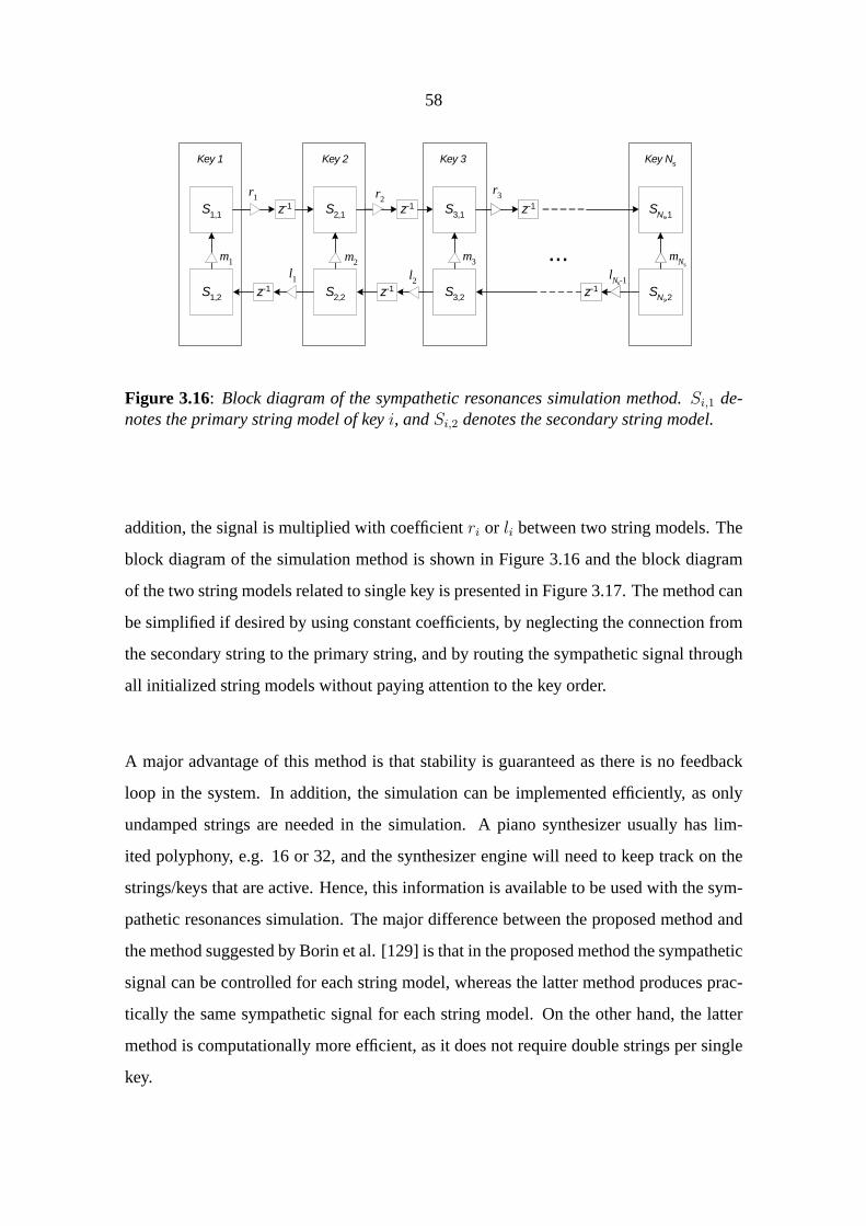
58

S2,1

S2,2

Key 2

S3,1

S3,2

Key 3

SN ,1

SN ,2

Key Ns

S1,1

S1,2

Key 1

r1 r2r3

lN -1l2l1...m1 m2 m3 mN

z-1 z-1z-1

z-1 z-1z-1

s

s

s

s

Figure 3.16: Block diagram of the sympathetic resonances simulation method.Si,1 de-notes the primary string model of keyi, andSi,2 denotes the secondary string model.

addition, the signal is multiplied with coefficientri or li between two string models. The

block diagram of the simulation method is shown in Figure 3.16 and the block diagram

of the two string models related to single key is presented in Figure 3.17. The method can

be simplified if desired by using constant coefficients, by neglecting the connection from

the secondary string to the primary string, and by routing the sympathetic signal through

all initialized string models without paying attention to the key order.

A major advantage of this method is that stability is guaranteed as there is no feedback

loop in the system. In addition, the simulation can be implemented efficiently, as only

undamped strings are needed in the simulation. A piano synthesizer usually has lim-

ited polyphony, e.g. 16 or 32, and the synthesizer engine will need to keep track on the

strings/keys that are active. Hence, this information is available to be used with the sym-

pathetic resonances simulation.The major difference between the proposed method and

the method suggested by Borin et al. [129] is that in the proposed method the sympathetic

signal can be controlled for each string model, whereas the latter method produces prac-

tically the same sympathetic signal for each string model. On the other hand, the latter

method is computationally more efficient, as it does not require double strings per single

key.

59

Excitation Stringmodel Excitation String

model

Sympathetic(outgoing)

Sympathetic(outgoing)

mn

String 2 String 1

output

Sympathetic(incoming)

Sympathetic(incoming)

Sympathetic left Sympathetic right

Figure 3.17: Block diagram of the sympathetic resonances simulation method of a singlekey.

Figure 3.18 shows an example of a synthetic piano tone simulated using Matlab with the

proposed sympathetic resonance method. In this example, keysE4 andG4 are pressed

down slowly in the beginning. Then, a loud staccato note is played on keyC2, which

causes the undamped string corresponding to the keysE4 andG4 to vibrate more loudly,

as desired. This suggests that the proposed method is able to simulate the phenomenon.

Corresponding sound examples can be found at http://lib.tkk.fi/Diss/2007/isbn9789512290666/.

3.6 Reference implementation with PWGL software

A real-time implementation of the piano synthesis model presented in this thesis is pre-

sented in [PVII]. The model is implemented with PWGL software [147, 148, 149, 150]

in collaboration with the Sibelius Academy and it does not use any sampled sounds for

producing sounds. The software implementation has two goals: to provide evidence that

the proposed new methods for piano synthesis can be implemented in real time, and to

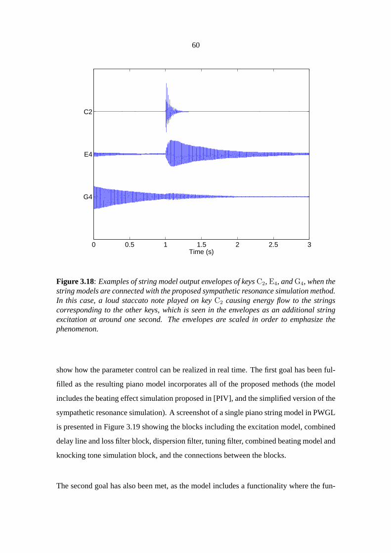
60

0 0.5 1 1.5 2 2.5 3

G4

E4

C2

Time (s)

Figure 3.18: Examples of string model output envelopes of keysC2, E4, andG4, when thestring models are connected with the proposed sympathetic resonance simulation method.In this case, a loud staccato note played on keyC2 causing energy flow to the stringscorresponding to the other keys, which is seen in the envelopes as an additional stringexcitation at around one second. The envelopes are scaled in order to emphasize thephenomenon.

show how the parameter control can be realized in real time. The first goal has been ful-

filled as the resulting piano model incorporates all of the proposed methods (the model

includes the beating effect simulation proposed in [PIV], and the simplified version of the

sympathetic resonance simulation). A screenshot of a single piano string model in PWGL

is presented in Figure 3.19 showing the blocks including the excitation model, combined

delay line and loss filter block, dispersion filter, tuning filter, combined beating model and

knocking tone simulation block, and the connections between the blocks.

The second goal has also been met, as the model includes a functionality where the fun-

61

damental frequency and the inharmonicity coefficient value of a single string can be mod-

ified in real time. Tuning certain parameters of a specific string is realized with a table,

where the parameter values can be changed on the fly. The new internal parameter values

for each block corresponding to a certain key are recalculated each time the key is pressed

down in the MIDI keyboard. Hence, it is possible to fine-tune e.g. the inharmonicity co-

efficient value by ear. An example of this is shown in Figure 14 of [PVII].

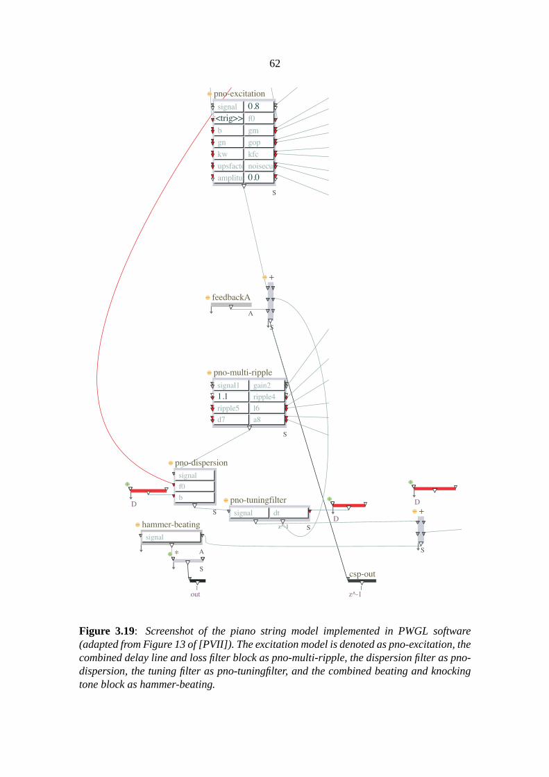
62

Anonymous 15

Computer Music Journal August 8, 2007

Figure 12 gives an overview of our system. This patch supports both real-time

and non-real-time modes: (1) MIDI mode (‘MIDI’) or (2) score mode (‘score’). The

current mode can be selected by using a master switch box having the label ‘MSW’

in the low-right corner of the box. The master switch box can have one or several

slave switch boxes that will follow the state of the master switch. Both the master

and slave switch boxes share the same box-string, which is in our case equal to

‘MIDI/score’.

Figure 13. Contents of the ‘string’ abstraction shown in Figure 12. Figure 3.19: Screenshot of the piano string model implemented in PWGL software(adapted from Figure 13 of [PVII]). The excitation model is denoted as pno-excitation, thecombined delay line and loss filter block as pno-multi-ripple, the dispersion filter as pno-dispersion, the tuning filter as pno-tuningfilter, and the combined beating and knockingtone block as hammer-beating.

63

4 Conclusions and future research directions

The theme of this thesis has been physics-based modeling of the piano. More specif-

ically, the development of new simulation methods that enable the implementation of

an efficient and parametrically controlled piano synthesis model. Work has been done

to develop methods for simulating the dispersion phenomenon, the string excitation, the

beating effect, and the sympathetic resonances phenomenon. As a result, a novel ex-

citation model has been proposed that is able to excite the string model in the desired

way while being able to maintain control of the model through parameters. Moreover,

the first closed-form design method for designing dispersion filters has been developed

for designing first- and second-order dispersion filters. In addition, an automatic analy-

sis algorithm for estimating the inharmonicity of piano tones has been developed to be

used to assist sound synthesis. Furthermore, two new amplitude modulation-based beat-

ing effect simulation methods have been suggested. These two methods can produce the

desired beating envelope efficiently and the methods can be controlled with parameters

in real time. Also, a new method for simulating the sympathetic resonances has been

introduced. Finally, these methods have been implemented in a real-time piano synthesis

model using the PWGL software proving that the goal for the work has been met.

As for future work, one of the main areas of research relates to the human perception

of piano tones, which provides essential information to be used in developing more effi-

cient and perceptually accurate sound synthesis models. At this moment, considering this

work, there is need for perceptual information related to dispersion filter design, loss filter

design, and excitation model calibration. Another interesting path of study is to investi-

gate how to implement piano synthesis models, which can be scaled in terms of memory

requirement and processor power, based on the parametric approach presented in this the-

sis. This work could be used, for example, in mobile phones and gaming devices. Finally,

an important part of the sound synthesis is the calibration of model parameters.The in-

troduced model could be used to develop an automatic calibration method that calibrates

64

the model based on a set of recorded piano tones.Hence, it would enable the simulation

of different pianos with the same model by obtaining different parameter sets for each

simulated piano.

65

References

[1] D. Rocchesso and F. Scalcon, “Bandwidth of perceived inharmonicity for phys-

ical modeling of dispersive strings,”IEEE Transactions on Speech and Audio

Processing, vol. 7, no. 5, pp. 597–601, 1999.

[2] P. Regalia and S. Mitra, “Tunable digital frequency response equalization filters,”

IEEE Transactions on Acoustics, Speech, and Signal Processing, vol. 35, no. 1,

pp. 118–120, 1987.

[3] J. O. Smith III, Physical Audio Signal Processing: for Virtual

Musical Instruments and Digital Audio Effects, August 2006 Edition,

http://ccrma.stanford.edu/˜jos/pasp06/ , Aug. 2006.

[4] J. O. Smith, “Virtual acoustic musical instruments: Review and update,”Journal

of New Music Research, vol. 33, no. 3, pp. 283–304, 2004.

[5] P. R. Cook, Real Sound Synthesis for Interactive Applications, A. K. Peters,

Natick, MA, 2002.

[6] D. A. Jaffe and J. O. Smith III, “Extensions of the Karplus-Strong plucked-string

algorithm,” Computer Music Journal, vol. 7, no. 2, pp. 76–87, 1983.

[7] J. O. Smith III, “Physical modeling using digital waveguides,”Computer Music

Journal, vol. 16, no. 4, pp. 74–91, 1992.

[8] L. Hiller and P. Ruiz, “Synthesizing musical sounds by solving the wave equation

for vibrating objects: Part 1,”Journal of the Audio Engineering Society, vol. 19,

no. 6, pp. 462–470, 1971.

[9] L. Hiller and P. Ruiz, “Synthesizing musical sounds by solving the wave equation

for vibrating objects: Part 2,”Journal of the Audio Engineering Society, vol. 19,

no. 7, pp. 542–551, 1971.

66

[10] H. Järveläinen,Perception of Attributes in Real and Synthetic String Instrument

Sounds, Ph.D. thesis, Helsinki University of Technology, Espoo, Finland, 2003.

[11] H. Järveläinen and M. Karjalainen, “Importance of inharmonicity in the acoustic

guitar,” in Proc. International Computer Music Conference, Barcelona, Spain,

2005, pp. 363–366.

[12] H. Järveläinen, V. Välimäki, and M. Karjalainen, “Audibility of the timbral ef-

fects of inharmonicity in stringed instrument tones,”Acoustics Research Letters

Online, vol. 2, no. 3, pp. 79–84, 2001.

[13] H. Järveläinen and M. Karjalainen, “Perception of beating and two-stage decay in

dual-polarization string models,” inProc. International Symposium on Musical

Acoustics, Mexico City, Mexico, 2002, pp. 1–10.

[14] H. Järveläinen, T. Verma, and V. Välimäki, “Perception and adjustment of pitch

in inharmonic string instrument tones,”Journal of New Music Research, vol. 31,

no. 3, pp. 311–319, 2002.

[15] H. Järveläinen and M. Karjalainen, “Perceptibility of inharmonicity in the acous-

tic guitar,” Acta Acustica united with Acustica, vol. 92, no. 5, pp. 842–847, 2006.

[16] A. Klapuri, Signal Processing Methods for the Automatic Transcription of Music,

Ph.D. thesis, Tampere University of Technology, Finland, 2004.

[17] A. Klapuri and M. Davy, Eds.,Signal Processing Methods for Music Transcrip-

tion, Springer-Verlag, New York, 2006.

[18] T. Virtanen, Sound Source Separation in Monaural Music Signals, Ph.D. thesis,

Tampere University of Technology, Finland, 2006.

[19] J. Rauhala and V. Välimäki, “F0 estimation of inharmonic piano tones using

partial frequencies method,” inProc. International Computer Music Conference,

Copenhagen, Denmark, 2007, pp. 453–456.

67

[20] N. H. Fletcher and T. D. Rossing,The Physics of Musical Instruments, Springer-

Verlag, New York, 1991.

[21] G. Weinreich, “Coupled piano strings,”Journal of the Acoustical Society of

America, vol. 62, no. 6, pp. 1474–1484, 1977.

[22] H. A. Conklin, “Piano strings and "phantom" partials,”Journal of the Acoustical

Society of America, vol. 102, no. 1, pp. 659, 1997.

[23] H. A. Conklin, “Generation of partials due to nonlinear mixing in a stringed

instrument,” Journal of the Acoustical Society of America, vol. 105, no. 1, pp.

536–545, 1999.

[24] B. Bank and L. Sujbert, “Generation of longitudinal vibrations in piano strings:

From physics to sound synthesis,”Journal of the Acoustical Society of America,

vol. 117, no. 4, pp. 2268–2278, 2005.

[25] A. Askenfelt, Ed.,Five Lectures on the Acoustics of the Piano, Royal Swedish

Academy of Music No. 64, Stockholm, Sweden, 1990.

[26] A. Askenfelt and E. V. Jansson, “From touch to string vibrations. I: Timing in the

grand piano action,”Journal of the Acoustical Society of America, vol. 88, no. 1,

pp. 52–63, 1990.

[27] H. Suzuki and I. Nakamura, “Acoustics of pianos,”Applied Acoustics, vol. 30,

no. 2–3, pp. 147–205, 1990.

[28] H. A. Conklin Jr., “Design and tone in the mechanoacoustic piano. part II. Piano

structure,” Journal of the Acoustical Society of America, vol. 100, no. 2, pp.

695–708, 1996.

[29] A. Askenfelt and E. V. Jansson, “From touch to string vibrations. II: The motion

of the key and hammer,”Journal of the Acoustical Society of America, vol. 90,

no. 5, pp. 2383–2393, 1991.

68

[30] H. A. Conklin Jr., “Design and tone in the mechanoacoustic piano. part I. Piano

hammers and tonal effects,”Journal of the Acoustical Society of America, vol.

99, no. 6, pp. 3286–3296, 1996.

[31] A. Stulov, “Experimental and computational studies of piano hammers,”Acta

Acustica united with Acustica, vol. 91, no. 2005, pp. 1086–1097, 2005.

[32] D. E. Hall, “Piano string excitation in the case of small hammer mass,”Journal

of the Acoustical Society of America, vol. 79, no. 1, pp. 141–147, 1986.

[33] D. E. Hall, “Piano string excitation II: General solution for a hard narrow ham-

mer,” Journal of the Acoustical Society of America, vol. 81, no. 2, pp. 535–546,

1987.

[34] D. E. Hall, “Piano string excitation III: General solution for a soft narrow ham-

mer,” Journal of the Acoustical Society of America, vol. 81, no. 2, pp. 547–555,

1987.

[35] D. E. Hall and P. Clark, “Piano string excitation IV: The question of missing

modes,” Journal of the Acoustical Society of America, vol. 82, no. 6, pp. 1913–

1918, 1987.

[36] D. E. Hall and A. Askenfelt, “Piano string excitation V: Spectra for real hammers

and strings,” Journal of the Acoustical Society of America, vol. 83, no. 4, pp.

1627–1638, 1988.

[37] D. E. Hall, “Piano string excitation VI: Nonlinear modeling,”Journal of the

Acoustical Society of America, vol. 92, no. 1, pp. 95–105, 1992.

[38] D. E. Hall, “String excitation: piano, harpsichord and clavichord,” inProc.

Stockholm Music Acoustics Conference, Stockholm, Sweden, 1993, pp. 309–314.

[39] A. Askenfelt and E. V. Jansson, “From touch to string vibrations. III: String

motion and spectra,”Journal of the Acoustical Society of America, vol. 93, no. 4,

pp. 2181–2196, 1993.

69

[40] H. A. Conklin Jr., “Design and tone in the mechanoacoustic piano. part III. Piano

strings and scale design,”Journal of the Acoustical Society of America, vol. 100,

no. 3, pp. 1286–1298, 1996.

[41] N. Giordano and A. J. Korty, “Motion of a piano string: Longitudinal vibrations

and the role of the bridge,”Journal of the Acoustical Society of America, vol.

100, no. 6, pp. 3899–3908, 1996.

[42] J.-L. Le Carrou, F. Gautier, N. Dauchez, and J. Gilbert, “Modelling of sympa-

thetic string vibrations,”Acta Acustica united with Acustica, vol. 91, no. 2, pp.

277–288, 2005.

[43] T. H. Moore and S. A. Zietlow, “Interferometric studies of a piano soundboard,”

Journal of the Acoustical Society of America, vol. 119, no. 3, pp. 1783–1793,

2006.

[44] I. Bork, “Sound radiation from a grand piano,” in100th AES Convention, Preprint

4158, Copenhagen, Denmark, 1996, pp. 1–4.

[45] J. Berthaut, M. N. Ichchou, and L. Jezequel, “Piano soundboard: structural be-

havior, numerical and experimental study in the modal range,”Applied Acoustics,

vol. 64, no. 11, pp. 1113–1136, 2003.

[46] N. Giordano, “Mechanical impedance of a piano soundboard,”Journal of the

Acoustical Society of America, vol. 103, no. 4, pp. 2128–2133, 1998.

[47] M. Keane, “Separation of piano keyboard vibrations into tonal and broadband

components,”Applied Acoustics, vol. 68, no. 10, pp. 1104–1117, 2007.

[48] I. Nakamura and D. Naganuma, “Characteristics of piano sound spectra,” inProc.

Stockholm Music Acoustics Conference, Stockholm, Sweden, 1993, pp. 325–330.

[49] A. Askenfelt, “Observations on the transient components of the piano tone,”

in Proc. Stockholm Music Acoustics Conference, Stockholm, Sweden, 1993, pp.

297–301.

70

[50] J. Smith, “Physical modeling synthesis update,”Computer Music Journal, vol.

20, no. 2, pp. 44–56, 1996.

[51] V. Välimäki, J. Huopaniemi, M. Karjalainen, and Z. Jánosy, “Physical model-

ing of plucked string instruments with application to real-time sound synthesis,”

Journal of the Audio Engineering Society, vol. 44, no. 5, pp. 331–353, 1996.

[52] V. Välimäki, “Physics-based modeling of musical instruments,”Acta Acustica

united with Acustica, vol. 90, no. 4, pp. 611–617, 2004.

[53] V. Välimäki, J. Pakarinen, C. Erkut, and M. Karjalainen, “Discrete-time mod-

elling of musical instruments,”Reports on Progress in Physics, vol. 69, no. 1, pp.

1–78, January 2006.

[54] A. Chaigne, “Numerical simulations of stringed instruments - today’s situation

and trends for the future,”Catgut Acoustical Society Journal, vol. 4, no. 5, pp.

12–20, 2002.

[55] T. Tolonen, V. Välimäki, and M. Karjalainen, “Evaluation of modern sound syn-

thesis methods,” Tech. Rep. 48, Laboratory of Acoustics and Audio Signal Pro-

cessing, Helsinki University of Technology, Espoo, Finland, 1998.

[56] C. Cadoz, A. Luciani, and J. Florens, “Responsive input devices and sound syn-

thesis by simulation of instrumental mechanisms: the CORDIS system,”Com-

puter Music Journal, vol. 8, no. 3, pp. 60–73, 1983.

[57] A. Fettweis, “Wave digital filters: Theory and practice,”Proceedings of the IEEE,

vol. 74, no. 2, pp. 270–327, June 1986.

[58] S. Bilbao,Wave and Scattering Methods for the Numerical Integration of Partial

Differential Equations, Ph.D. thesis, Stanford University, CA, 2001.

[59] J. M. Adrien, “Dynamic modeling of vibrating structures for sound synthesis,

modal synthesis,” inProc. AES 7th International Conference, Toronto, Canada,

1989, Audio Engineering Society, pp. 291–300.

71

[60] J.-M. Adrien, “The missing link: modal synthesis,” inRepresentations of Musical

Signals, G. De Poli, A. Piccialli, and C. Roads, Eds., pp. 269–297. The MIT Press,

Cambridge, Massachusetts, 1991.

[61] L. Trautmann and R. Rabenstein, “Digital sound synthesis based on transfer

function models,” inProc. IEEE Workshop on Applications of Signal Processing

to Audio and Acoustics, New Paltz, New York, 1999, pp. 83–86.

[62] R. Rabenstein and L. Trautmann, “Digital sound synthesis of string instruments

with the functional transformation method,”Signal Processing, vol. 83, no. 8, pp.

1673–1688, 2003.

[63] C. Roads, The Computer Music Tutorial, The MIT Press, Cambridge, Mas-

sachusetts, USA, 1995.

[64] J. A. Moorer, “Signal processing aspects of computer music: A survey,”Pro-

ceedings of the IEEE, vol. 65, no. 8, pp. 1108–1137, 1977.

[65] A. Chaigne and A. Askenfelt, “Numerical simulations of piano strings. I. A phys-

ical model for a struck string using finite difference methods,”Journal of the

Acoustical Society of America, vol. 95, no. 2, pp. 1112–1118, 1994.

[66] A. Chaigne and A. Askenfelt, “Numerical simulations of piano strings. II. Com-

parisons with measurements and systematic exploration of some hammer-string

parameters,” Journal of the Acoustical Society of America, vol. 95, no. 3, pp.

1631–1640, 1994.

[67] N. Giordano and M. Jiang, “Physical modeling of the piano,”EURASIP Journal

of Applied Signal Processing, vol. 2004, no. 7, pp. 926–933, 2004.

[68] B. Bank and L. Sujbert, “Modeling the longitudinal vibration of piano strings,”

in Proc. Stockholm Music Acoustics Conference, Stockholm, Sweden, 2003, pp.

143–146.

72

[69] J. Laroche and J.-L. Meillier, “Multichannel excitation/filter modeling of percus-

sive sounds with application to the piano,”IEEE Transactions on Speech and

Audio Processing, vol. 2, no. 2, pp. 329–344, 1994.

[70] B. Hamadicharef and E. Ifeachor, “Perceptual modeling of piano tones,” in119th

AES Convention, Preprint 6525, New York, NY, 2005, pp. 1–8.

[71] S. A. Van Duyne, J. R. Pierce, and J. O. Smith, “Traveling-wave implementation

of a lossless mode-coupling filter and the wave digital hammer,” inProc. Inter-

national Computer Music Conference, Aarhus, Denmark, 1994, pp. 411–418.

[72] K. Karplus and A. Strong, “Digital synthesis of plucked-string and drum timbres,”

Computer Music Journal, vol. 7, no. 2, pp. 43–55, 1983.

[73] V. Välimäki and T. Tolonen, “Development and calibration of a guitar synthe-

sizer,” Journal of the Audio Engineering Society, vol. 46, no. 9, pp. 766–778,

1998.

[74] M. Laurson, C. Erkut, V. Välimäki, and M. Kuuskankare, “Methods for modeling

realistic playing in acoustic guitar synthesis,”Computer Music Journal, vol. 25,

no. 3, pp. 38–49, 2001.

[75] H. Penttinen, Loudness and Timbre Issues in Plucked Stringed Instruments -

Analysis, Synthesis, and Design, Ph.D. thesis, Helsinki University of Technology,

Espoo, Finland, 2006.

[76] E. Rank and G. Kubin, “A waveguide model for slapbass synthesis,” inProc.

IEEE International Conference on Acoustics, Speech, and Signal Processing, Mu-

nich, Germany, 1997, pp. 443–446.

[77] V. Välimäki, M. Karjalainen, T. Tolonen, and C. Erkut, “Nonlinear modeling

and synthesis of the kantele a traditional Finnish string instrument,” inProc.

International Computer Music Conference, Beijing, China, 1999, pp. 22–28.

73

[78] M. Karjalainen, V. Välimäki, and Z. Jánozy, “Towards high-quality sound syn-

thesis of guitar and string instruments,” inProc. International Computer Music

Conference, Tokyo, Japan, 1993, pp. 64–71.

[79] H. Penttinen, J. Pakarinen, V. Välimäki, M. Laurson, H. Li, and M. Leman,

“Model-based sound synthesis of the guqin,”Journal of the Acoustical Society of

America, vol. 120, no. 6, pp. 4052–4063, 2006.

[80] C. Erkut and V. Välimäki, “Model-based sound synthesis of tanbur, a Turkish

long-necked lute,” inProc. IEEE International Conference on Acoustics, Speech,

and Signal Processing, Istanbul, Turkey, 2000, pp. 769–772.

[81] C. Erkut, M. Laurson, V. Välimäki, and M. Kuuskankare, “Model-based synthe-

sis of the ud and the Renaissance lute,” inProc. International Computer Music

Conference, Havana, Cuba, 2001, pp. 119–122.

[82] C. Erkut, T. Tolonen, M. Karjalainen, and V. Välimäki, “Acoustical analysis of

tanbur, a Turkish long-necked lute,” inProc. Sixth International Congress on

Sound and Vibration, Lyngby, Denmark, 1999, pp. 345–352.

[83] C. Erkut, M. Karjalainen, P. Huang, and V. Välimäki, “Acoustical analysis and

model-based sound synthesis of the kantele,”Journal of the Acoustical Society of

America, vol. 112, no. 4, pp. 1681–1691, 2002.

[84] C. Erkut,Aspects in Analysis and Model-Based Sound Synthesis of Plucked String

Instruments, Ph.D. thesis, Helsinki University of Technology, Espoo, Finland,

2002.

[85] V. Välimäki, T. I. Laakso, M. Karjalainen, and U. K. Laine, “A new computational

model for the clarinet,” inProc. International Computer Music Conference, San

Francisco, CA, 1992.

[86] V. Välimäki, M. Karjalainen, Z. Jánosy, and U. K. Laine, “A real-time DSP

implementation of a flute model,” inProc. IEEE International Conference on

74

Acoustics, Speech, and Signal Processing, San Francisco, CA, 1992, pp. 249–

252.

[87] D. Rocchesso and F. Turra, “A generalized excitation for real-time sound syn-

thesis by physical models,” inProc. Stockholm Music Acoustics Conference,

Stockholm, Sweden, 1993, pp. 584–588.

[88] P. R. Cook, “Tbone: an interactive waveguide brass instrument synthesis work-

bench for the next machine,” inProc. International Computer Music Conference,

Montreal, Canada, 1991, pp. 297–299.

[89] C. Vergez and X. Rodet, “Comparison of real trumpet playing, latex model of

lips and computer model,” inProc. International Computer Music Conference,

Thessaloniki, Greece, 1997, pp. 180–187.

[90] J. O. Smith III, Techniques for Digital Filter Design and System Identification

with Application to the Violin, Ph.D. thesis, Dept. of Music, Stanford University,

Stanford, CA, 1983.

[91] J. Smith, “Nonlinear commuted synthesis of bowed strings,” inProc. Interna-

tional Computer Music Conference, Thessaloniki, Greece, 1997, pp. 264–267.

[92] S. Serafin and J. O. Smith, “Impact of string stiffness on digital waveguide models

of bowed strings,”Catgut Acoustical Society Journal, vol. 4, no. 4, pp. 49–52,

2001.

[93] S. Serafin, The Sound of Friction: Real-time Models, Playability and Musical

Applications, Ph.D. thesis, Stanford University, CA, 2004.

[94] V. Välimäki, M. Laurson, and C. Erkut, “Commuted waveguide synthesis of the

clavichord,” Computer Music Journal, vol. 27, no. 1, pp. 71–82, 2003.

[95] V. Välimäki, H. Penttinen, J. Knif, M. Laurson, and C. Erkut, “Sound synthesis

of the harpsichord using a computationally efficient physical model,”EURASIP

Journal of Applied Signal Processing, vol. 4, no. 7, pp. 934–948, 2004.

75

[96] G. E. Garnett, “Modeling piano sound using waveguide digital filtering tech-

niques,” inProc. International Computer Music Conference, Urbana, USA, 1987,

pp. 89–95.

[97] S. A. Van Duyne, Digital Filter Applications to Wave Propagation in Springs,

Strings, Membranes and Acoustical Space, Ph.D. thesis, Stanford University,

CA, 2007.

[98] S. A. Van Duyne and J. O. Smith III, “A simplified approach to modeling disper-

sion caused by stiffness in strings and plates,” inProc. International Computer

Music Conference, Århus, Denmark, 1994, pp. 407–410.

[99] S. A. Van Duyne and J. O. Smith, “Developments for the commuted piano,” in

Proc. International Computer Music Conference, Banff, Canada, 1995, pp. 335–

343.

[100] J. O. Smith and S. A. Van Duyne, “Commuted piano synthesis,” inProc. Inter-

national Computer Music Conference, Banff, Canada, 1995, pp. 319–326.

[101] J. O. Smith and S. A. Van Duyne, “Overview of the commuted piano synthesis

technique,” inProc. IEEE Workshop on Applications of Signal Processing to

Audio and Acoustics, New Paltz, New York, 1995, pp. 319–326.

[102] M. Aramaki, J. Bensa, L. Daudet, Ph. Guillemain, and R. Kronland-Martinet,

“Resynthesis of coupled piano string vibrations based on physical modeling,”

Journal on New Music Research, vol. 30, no. 3, pp. 213–226, 2001.

[103] J. Bensa, S. Bilbao, R. Kronland-Martinet, and J. O. Smith, “From the physics

of piano strings to digital waveguides,” inProc. International Computer Music

Conference, Göteborg, Sweden, 2002, pp. 45–48.

[104] J. Bensa, S. Bilbao, R. Kronland-Martinet, and J. O. Smith, “The simulation of

piano string vibration: From physical models to finite difference schemes and

digital waveguides,”Journal of the Acoustical Society of America, vol. 114, no.

2, pp. 1095–1107, 2003.

76

[105] J. Bensa, Analysis and Synthesis of Piano Sounds using Physical and Signal

Models, Ph.D. thesis, Université de la Méditérranée, France, 2003.

[106] J. Bensa, S. Bilbao, R. Kronland-Martinet, J. O. Smith, and T. Voinier, “Compu-

tational modeling of stiff piano strings using digital waveguides and finite differ-

ences,”Acta Acustica united with Acustica, vol. 91, no. 2, pp. 289–298, 2005.

[107] J. Bensa, S. Bilbao, R. Kronland-Martinet, and J. O. Smith, “A power normal-

ized non-linear lossy piano hammer,” inStockholm Music Acoustics Conference,

Stockholm, Sweden, 2003, pp. 365–368.

[108] J. Bensa, F. Gibaudan, K. Jensen, and R. Kronland-Martinet, “Note and hammer

velocity dependance of a piano string model based on coupled digital waveg-

uides,” inProc. International Computer Music Conference, Havana, Cuba, 2001,

pp. 95–98.

[109] J. Bensa, K. Jensen, and R. Kronland-Martinet, “A hybrid resynthesis model for

hammer-strings interaction of piano tones,”EURASIP Journal of Applied Signal

Processing, vol. 2004, no. 7, pp. 1021–1035, 2004.

[110] J. Bensa and L. Daudet, “Efficient modeling of "phantom" partials in piano tones,”

in International Symposium on Musical Acoustics, Nara, Japan, 2004.

[111] B. Bank, Physics-based Sound Synthesis of String Instruments Including Ge-

ometric Nonlinearities, Ph.D. thesis, Budapest University of Technology and

Economics, Budapest, Hungary, 2006.

[112] B. Bank, “Nonlinear interaction in the digital waveguide with the application

to piano sound synthesis,” inProc. International Computer Music Conference,

Berlin, Germany, 2000, pp. 54–58.

[113] B. Bank and L. Sujbert, “On the nonlinear commuted synthesis of the piano,”

in Proc. International Conference on Digital Audio Effects, Hamburg, Germany,

2002, pp. 175–180.

77

[114] B. Bank, V. Välimäki, L. Sujbert, and M. Karjalainen, “Efficient physics based

sound synthesis of the piano using DSP methods,” inEuropean Signal Processing

Conference, Tampere, Finland, 2000, pp. 2225–2228.

[115] B. Bank, “Accurate and efficient method for modeling beating and two-stage

decay in string instrument synthesis,” inMOSART Workshop on Current Research

Directions in Computer Music, Barcelona, Spain, 2001, pp. 124–133.

[116] B. Bank, “Physics-based sound synthesis of the piano,” M.S. thesis, Budapest

University of Technology and Economics, Budapest, Hungary, 2000.

[117] B. Bank and V. Välimäki, “Robust loss filter design for digital waveguide syn-

thesis of string tones,”IEEE Signal Processing Letters, vol. 10, no. 1, pp. 18–20,

2003.

[118] B. Bank and L. Sujbert, “A piano model including longitudinal string vibrations,”

in Proc. International Conference on Digital Audio Effects, Naples, Italy, 2004,

pp. 89–94.

[119] B. Bank, F. Avanzini, G. Borin, G. De Poli, F. Fontana, and D. Rocchesso, “Phys-

ically informed signal processing methods for piano sound synthesis: A research

overview,” EURASIP J. App. Sig. Proc., vol. 2003, no. 10, pp. 941–952, 2003.

[120] F. Avanzini, B. Bank, G. Borin, G. De Poli, F. Fontana, and D. Rocchesso, “Mu-

sical instrument modeling: The case of the piano,” inMOSART Workshop on

Current Research Directions in Computer Music, Barcelona, Spain, 2001, pp.

124–133.

[121] M. Karjalainen, V. Välimäki, and T. Tolonen, “Plucked-string models: from the

karplus-strong algorithm to digital waveguides and beyond,”Computer Music

Journal, vol. 22, no. 3, pp. 17–32, 1998.

[122] J. O. Smith, “Efficient synthesis of stringed musical instruments,” inProc. Inter-

national Computer Music Conference, Tokyo, Japan, 1993, pp. 64–71.

78

[123] N. Lee, Z. Duan, and J. O. Smith III, “Excitation extraction for guitar tones,” in

Proc. International Computer Music Conference, Copenhagen, Denmark, 2007,

pp. 450–457.

[124] J. Rauhala, H.-M. Lehtonen, and V. Välimäki, “Multi-ripple loss filter for

waveguide piano synthesis,” inProc. International Computer Music Conference,

Barcelona, Spain, 2005, pp. 729–732.

[125] T. I. Laakso, V. Välimäki, M. Karjalainen, and U. K. Laine, “Splitting the unit

delay - tools for fractional delay filter design,”IEEE Signal Processing Magazine,

vol. 13, no. 1, pp. 30–60, 1996.

[126] D. Rocchesso and F. Scalcon, “Accurate dispersion simulation for piano strings,”

in Proc. Nordic Acoustical Meeting, Helsinki, Finland, 1996, pp. 407–414.

[127] H.-M. Lehtonen, “Analysis and parametric synthesis of the piano sound,” M.S.

thesis, Helsinki University of Technology, Espoo, Finland, 2005.

[128] H.-M. Lehtonen, H. Penttinen, J. Rauhala, and V. Välimäki, “Analysis and model-

ing of piano sustain-pedal effects,”Journal of the Acoustical Society of America,

vol. 122, no. 3, pp. 1787–1797, 2007.

[129] G. Borin, D. Rocchesso, and F. Scalcon, “A physical piano model for music

performance,” inProc. International Computer Music Conference, Thessaloniki,

Greece, 1997, pp. 350–353.

[130] B. E. Anderson and W. J. Strong, “The effect of inharmonic partials on pitch of

piano tones,”Journal of the Acoustical Society of America, vol. 117, no. 5, pp.

3268–3272, 2005.

[131] V. Välimäki, Discrete-Time Modeling of Acoustic Tubes Using Fractional Delay

Filters, Ph.D. thesis, Helsinki University of Technology, 1995.

[132] H.-M. Lehtonen, J. Rauhala, and V. Välimäki, “Sparse multi-stage loss filter

design for waveguide piano synthesis,” inIEEE Workshop on Applications of

79

Signal Processing to Audio and Acoustics, New Paltz, New York, 2005, pp. 331–

334.

[133] G. Borin, G. De Poli, and D. Rocchesso, “Elimination of delay-free loops

in discrete-time models of nonlinear acoustic systems,”IEEE Transactions on

Speech and Audio Processing, vol. 8, no. 5, pp. 597–605, 2000.

[134] S. Van Duyne and J. O. Smith, “The wave digital hammer: A traveling wave

model of the piano hammer and the felt mallet,” inProc. International Computer

Music Conference, Århus, Denmark, 1994, pp. 411–418.

[135] E. D. Blackham, “The physics of the piano,”Scientific American, vol. 213, no. 6,

pp. 88–96, 1965.

[136] A. Galembo, “Quality of treble piano tones,” inProc. Stockholm Music Acoustics

Conference, Stockholm, Sweden, 2003, pp. 146–150.

[137] L. Ortiz-Berenguer, J. Casajus-Quiros, M. Torres-Guijarro, J. Beracoechea, and

J. Perez-Aranda, “Simple modeling of piano inharmonicity due to soundboard

impedance,” in120th AES Convention, Preprint 6647, Paris, France, 2006, pp.

1–6.

[138] J. Woodhouse, “Plucked guitar transients: comparison of measurements and syn-

thesis,”Acta Acustica united with Acustica, vol. 90, no. 5, pp. 945–965, 2004.

[139] H. Fletcher, E. D. Blackham, and R. Stratton, “Quality of piano tones,”Journal

of the Acoustical Society of America, vol. 34, no. 6, pp. 749–761, 1962.

[140] A. Galembo, A. Askenfelt, L. L. Cuddy, and F. A. Russo, “Perceptual relevance

of inharmonicity and spectral envelope in the piano bass range,”Acta Acustica

united with Acustica, vol. 90, no. 3, pp. 528–536, 2004.

[141] A. S. Galembo and A. Askenfelt, “Signal representation and estimation of spec-

tral parameters by inharmonic comb filters with application to the piano,”IEEE

Transactions on Speech and Audio Processing, vol. 7, no. 2, pp. 197–203, 1999.

80

[142] A. Askenfelt and A. S. Galembo, “Study of the spectral inharmonicity of musical

sound by the algorithms of pitch extraction,”Acoustical Physics, vol. 46, no. 2,

pp. 121–132, 2000.

[143] J.-P. Thiran, “Recursive digital filters with maximally flat group delay,”IEEE

Transactions on Circuit Theory, vol. 18, no. 6, pp. 659–664, 1971.

[144] A. Fettweis, “A simple design of maximally flat delay digital filters,”IEEE

Transactions on Audio and Electroacoustics, vol. 20, no. 2, pp. 112–114, 1972.

[145] M. Lang and T. I. Laakso, “Simple and robust method for the design of allpass

filters using least-squares phase error criterion,”IEEE Transactions on Circuits

and Systems, vol. 41, no. 1, pp. 40–48, 1994.

[146] B. Capleton, “False beats in coupled piano string unisons,”Journal of the Acous-

tical Society of America, vol. 115, no. 2, pp. 885–892, 2004.

[147] M. Laurson, V. Norilo, and M. Kuuskankare, “PWGLSynth: A visual synthesis

language for virtual instrument design and control,”Computer Music Journal,

vol. 29, no. 3, pp. 29–41, 2005.

[148] M. Kuuskankare and M. Laurson, “Expressive notation package,”Computer

Music Journal, vol. 30, no. 4, pp. 67–79, 2006.

[149] M. Laurson and M. Kuuskankare, “Recent trends in PWGL,” inProc. Interna-

tional Computer Music Conference, New Orleans, LA, 2006, pp. 258–261.

[150] M. Laurson and V. Norilo, “From score-based approach towards real-time con-

trol in PWGLSynth,” inProc. International Computer Music Conference, New

Orleans, LA, 2006, pp. 29–32.