Physics without fundamental time

Carlo Rovelli

I. Time, who?

II. Physics without fundamental time

III. A real world example

What are we talking about when we talk about

time?

Descartes: Res extensa

Aristotle : (Changing) Substance

Einstein 05: Spacetime

Einstein 15: Covariant fields

Faraday-Maxwell: Fields Particles

Quantum: Quantum Fields

Newton: Time Space Particles

Quantum gravity?: Covariant Quantum Fields

Change is “the actuality of that which potentially is, qua such” (Aristotle Physics 201a9-11)

Time is “a number of change” (Aristotle Physics 219b1)

data theories

Scientist

Conceptual framework

(Space, time, reality, causality, observation, objectivity, language,…)

improve evolve

evolve as well!

Non foundationalism: - There is no final scientific theory of the world. - There is no definitive metaphysics. We learn.

General relativity “takes away from space and time the last remnant of physical objectivity”

A Einstein, The foundations of general relativity, 1916

“On the basis of general relativity, space, as opposed to “what fills space”, has no separate existence.

If we imagine the gravitational field to be removed, there does not remain a space [...], but absolutely nothing.

A Einstein, Relativity, the special and general theory, 1917

Time =

Z

�d⌧

rgµ⌫(�(⌧))

d�µ

d⌧

d�⌫

d⌧

gravitational field

ΔΤ = Τ2 - Τ1

Τ2

Τ1

Thermodynamical (and common sense): oriented, metric, universal

Classical and quantum mechanical: metric, universal

Special relativistic, quantum field theoretical: metric, frame dependent

Quantum gravity: none

Dynamics on curved spacetime: metric, path dependent

Dynamics of gravitational field: relational

Negligible quantum gravity effects

Negligible backreaction

Low curvature

Low relative velocities

Special initial conditionsor special observer

Times in physics:

Can we do physics, without time?

Of course yes! Lagrange, …, Dirac, Souriau, Arnold,…DeWitt, …

Quantum gravity Carlo Rovelli CUP 2004

Introduction to Canonical Loop Quantum Gravity Francesca Vidotto, Carlo Rovelli CUP 2014

d

2x(t)

dt

2= �!

2x(t)

Position (dependent variable):

Time (independent variable):

Equations of motion:

General solution (motions):

t 2 R

x 2 C

x(t) = A sin(!t+ �)

x

t

Variables (dependent and independent not distinguished):

Equations of motion:

General solution (motions):

dx� p dt = 0; dp+ !

2x dt = 0

f(x, t) = x�A sin(!t+ �) = 0

Time and configuration variables can be treated on equal footings.

partial observablesx

t

(x, t) 2 E = C ⇥R

Cfr: SeanCfr: Brian

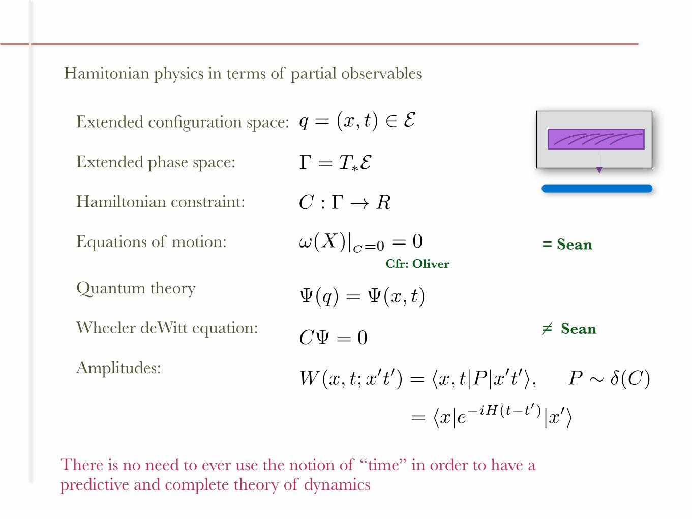
Hamitonian physics in terms of partial observables

� = T⇤E

C : � ! R

!(X)|C=0 = 0

q = (x, t) 2 E

There is no need to ever use the notion of “time” in order to have a predictive and complete theory of dynamics

Extended configuration space:

Extended phase space:

Hamiltonian constraint:

Equations of motion: = SeanCfr: Oliver

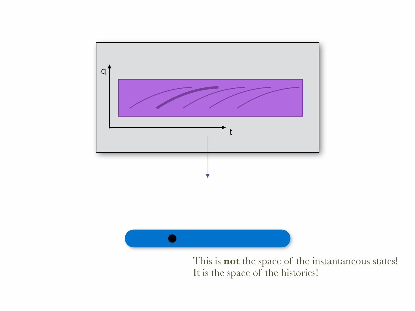
This is not the space of the instantaneous states! It is the space of the histories!

q

t

� = T⇤E

C : � ! R

!(X)|C=0 = 0

q = (x, t) 2 E

There is no need to ever use the notion of “time” in order to have a predictive and complete theory of dynamics

Quantum theory

Wheeler deWitt equation:

Amplitudes:

(q) = (x, t)

C = 0

W (x, t;x0t

0) = hx, t|P |x0t

0i, P ⇠ �(C)

= hx|e�iH(t�t0)|x0i

Extended configuration space:

Extended phase space:

Hamiltonian constraint:

Equations of motion: = Sean

= Sean

Hamitonian physics in terms of partial observables

Cfr: Oliver

This is not the space of the instantaneous states! It is the space of the histories!

q

q’

Classical and quantum physics without time

� = T⇤E

C : � ! R

!(X)|C=0 = 0

q = (x, t) 2 E

There is no need to ever use the notion of “time” in order to have a predictive and complete theory of dynamics

Quantum theory

Wheeler deWitt equation:

Amplitudes:

(q) = (x, t)

C = 0

W (x, t;x0t

0) = hx, t|P |x0t

0i, P ⇠ �(C)

= hx|e�iH(t�t0)|x0i

Extended configuration space:

Extended phase space:

Hamiltonian constraint:

Equations of motion:

(x, t) ! q

q

set of all partial observables

q

qq ; q0 q0

q1 q’1q2 q’2q3 q’3q4 q’4… …

What needs to be diff invariant are the transition amplitudes between partial observables’s

eigenstates,

not the “observables” themselves!

Dynamics describes evolution of dynamical variables in time.

Dynamics describe relations between partial observables

This is possible for any dynamical system.

It is necessary for a system including gravity.

Please do not confuse:

xT (x, p, t, pt) =1

2(x2 + p

2) sin

✓!(T � t) + arctan

!x

p

◆

x̂T =1

2(x̂2 + p̂

2) sin

✓!(T � t̂) + arctan

!x̂

p̂

◆

Evolving constants of motion:

Quantum evolving constants Carlo Rovelli Physical Review D44, 1339 (1991)

xT = xT (x, p, t, pt)

x̂T = xT (x̂, p̂, t̂, p̂t)

Partial observables:

W (x, t;x0t

0) = hx, t|P |x0t

0i, P ⇠ �(C)Quantum Gravity Carlo Rovelli (CUP 2004)

Covariant Loop Quantum Gravity Carlo Rovelli, Francesca Vidotto (CUP 2014)

f(x, p, t, pt;x0, p

0, t

0, p

0t) = 0

W (x, t, x0, t

0) =

✓m!

h sin(!(t� t

0)

◆1

2

e

� i

~

(x

2

+x

02) cos(!(t�t

0))�2xx

0

sin

2

(!(t�t

0))

�

Partial observable: Can be measured

Dirac observable: Can be predicted

What is “observable” in GR

is not controversial

because all experimenters agree

when they make general relativistic observations

General relativity:

• Spacetime is the physical trajectory the gravitational field.

Quantum theory:

• Physical trajectories do not exist. Processes are transitions.

There is no spacetime in quantum gravity, and in particular there is “no time”

“Spacetime region”

Boundary

A process, and its amplitude

A = W ( )

Boundary state

Amplitude of the process

For example, Loop Quantum Gravity gives a precise mathematical definition of the state of space, the boundary observables, and the amplitude functional. (Processes, not a frozen spacetime...)

= in

⌦ out

Cfr: Bianca

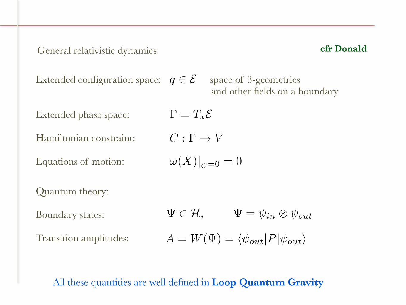
Extended configuration space: space of 3-geometries and other fields on a boundary

Extended phase space:

Hamiltonian constraint:

Equations of motion:

Quantum theory:

Boundary states:

Transition amplitudes:

General relativistic dynamics

� = T⇤E

!(X)|C=0 = 0

C : � ! V

q 2 E

2 H, = in

⌦ out

A = W ( ) = h out

|P | out

i

All these quantities are well defined in Loop Quantum Gravity

cfr Donald

hf =Y

v

hvf

State space

Operators: where Kine

mat

ics

8⇡�~G = 1

H� = L2[SU(2)L/SU(2)N ]�

�

spinfoam(vertices, edges, faces)

C

f

ev

3 (hl)

l

n

n0

�

hl

spin network(nodes, links)

Covariant loop quantum gravity. Full definition.B

ound

ary

Transition amplitudes

Vertex amplitude

Dyn

amic

s WC(hl) = NC

Z

SU(2)dhvf

Y

f

�(hf )Y

v

A(hvf )

A(hvf ) =

Z

SL(2,C)dg0e

Y

f

X

j

(2j + 1) Djmn(hvf )D

�(j+1) jjmjn (geg

�1e0 )

Bul

k

H = lim�!1

H�

W = limC!1

WC

- The notion of “Time” is not needed to describe change.

- The notion of “Time” is not of use, and in fact misleading, in relativistic quantum gravitational physics.

'

Σ

28

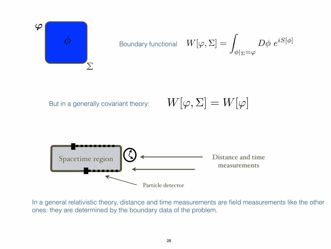
W [',⌃] =

Z

�|⌃='D� eiS[�]

Spacetime region

Particle detector

Distance and time measurements

In a general relativistic theory, distance and time measurements are field measurements like the other ones: they are determined by the boundary data of the problem.

But in a generally covariant theory: W [',⌃] = W [']

� Boundary functional

A concrete application

A technical result in classical GR:The following metric is an exact vacuum solution, plus an ingoing and outgoing shell, of the Einstein equations outside a finite spacetime region (grey).

ds2 = �F (u, v)dudv + r2(u, v)(d✓2 + sin2✓d�2)

F (uI , vI) = 1, rI(uI , vI) =vI � uI

2.Region I

vI < 0.

Region II F (u, v) =32m3

re

r2m

⇣1� r

2m

⌘e

r2m = uv.

rI(uI , vI) = r(u, v)Matching: u(uI

) =1

vo

⇣1 +

uI

4m

⌘e

uI4m .

F (uq, vq) =32m3

rqe

rq2m , rq = vq � uq.Region III

The metric is determined by three constants: m, ✏, �

I

III II

I

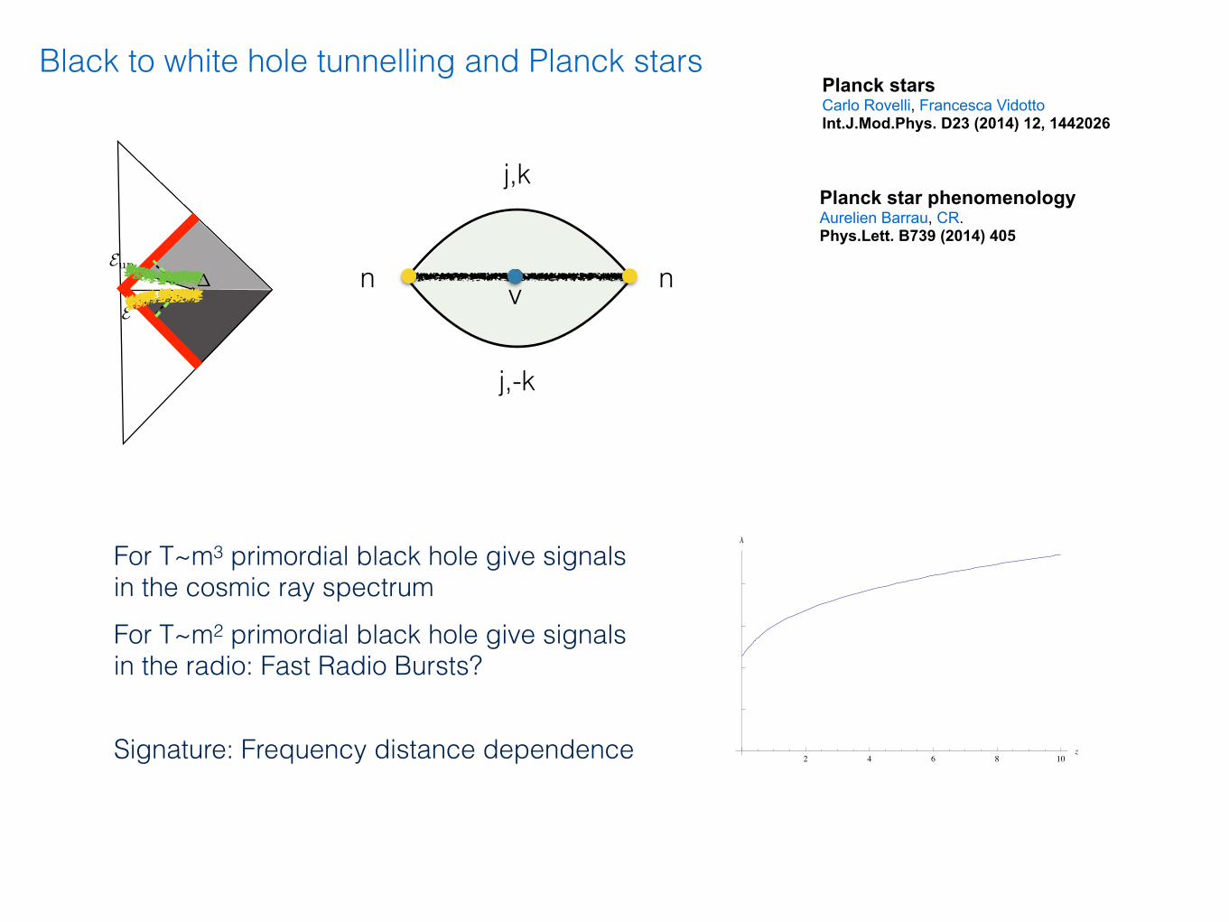
Black hole fireworks: quantum-gravity effects outside the horizon spark black to white hole tunneling Hal M. Haggard, Carlo Rovelli arXiv:1407.0989

I

I

Minkowski region

Schwarzschild region

Incoming (null) shell

Outgoing (null) shell

Future trapped horizonConventional black hole

Past trapped horizon

White hole

Minkowski region

IIIIIQuantum

region

The Fingers Crossed

➜

I

I

r=0

r=

ar=R

t = 0τ

u

v

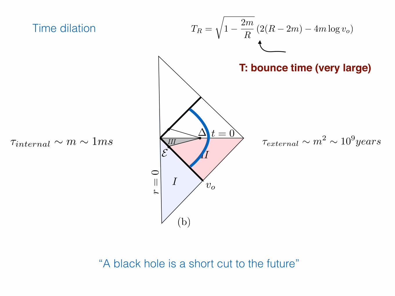
⌧internal ⇠ m ⇠ 1ms ⌧external

⇠ m2 ⇠ 109years

“A black hole is a short cut to the future”

Time dilation

T: bounce time (very large)

TR

=

r1� 2m

R(2(R� 2m)� 4m log v

o

)

vo

r=0

r=

ar=R

t = 0τ

u

v

⌧internal ⇠ m ⇠ 1ms ⌧external

⇠ m2 ⇠ 109years

“A black hole is a short cut to the future”

Time dilation

T: bounce time (very large)

TR

=

r1� 2m

R(2(R� 2m)� 4m log v

o

)

vo

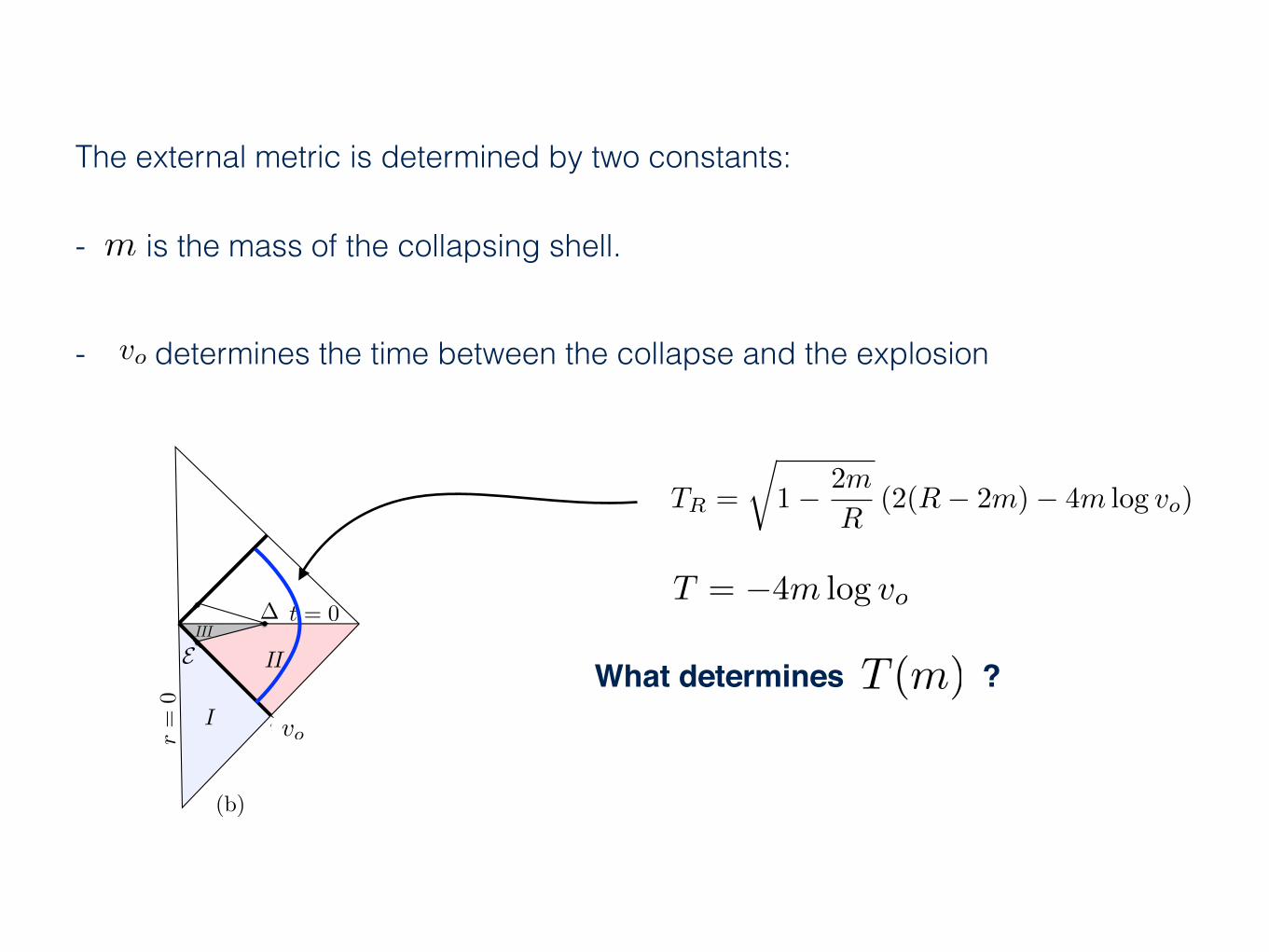
The external metric is determined by two constants:

- is the mass of the collapsing shell.m

- determines the time between the collapse and the explosion

What determines ? T (m)

r=0

r=

ar=R

t = 0τ

u

v

vo

TR

=

r1� 2m

R(2(R� 2m)� 4m log v

o

)

vo

T = �4m log vo

A(j, k) =

Z

SL(2C)dg

Z

SU2dh�

Z

SU2dh+

X

j+j�

e�(j+�j)2e�(j+�j)2

Trj+ [ek�3Y †gY ]Trj� [e

k�3Y †gY ]

|A(j, k)|2 ⇠ 1

T (m)

v nn

j,k

j,-k

relation j-krelation m-time

Covariant loop quantum gravity. Calculation of T(m).

v nn

j,k

j,-k

For T~m3 primordial black hole give signals in the cosmic ray spectrumFor T~m2 primordial black hole give signals in the radio: Fast Radio Bursts?

Planck star phenomenology Aurelien Barrau, CR. Phys.Lett. B739 (2014) 405

Signature: Frequency distance dependence 2 4 6 8 10z

l

Black to white hole tunnelling and Planck starsPlanck stars Carlo Rovelli, Francesca Vidotto Int.J.Mod.Phys. D23 (2014) 12, 1442026

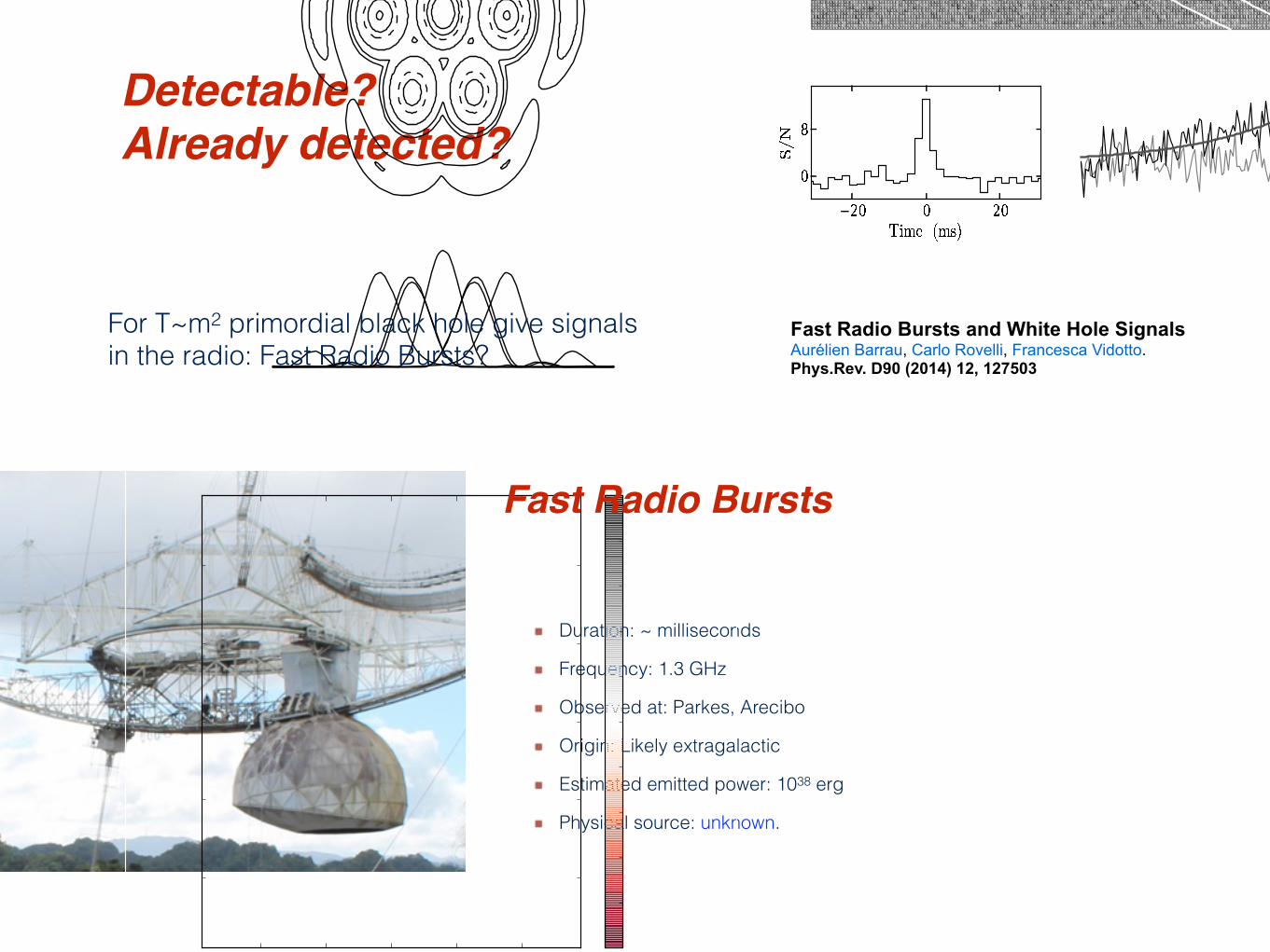
Detectable?Already detected?

Duration: ~ milliseconds

Frequency: 1.3 GHz

Observed at: Parkes, Arecibo

Origin: Likely extragalactic

Estimated emitted power: 1038 erg

Physical source: unknown.

4

Figure 1. Gain and spectral index maps for the ALFA receiver.Figure a): Contour plot of the ALFA power pattern calculatedfrom the model described in Section 3 at ν = 1375 MHz. Thecontour levels are −13, −10, −6, −3 (dashed), −2, and −1 dB(top panel). The bottom inset shows slices in azimuth for eachbeam, and each slice passes through the peak gain for its respec-tive beam. Beam 1 is in the upper right, and the beam number-ing proceeds clockwise. Beam 4 is, therefore, in the lower left.Figure b): Map of the apparent instrumental spectral index dueto frequency-dependent gain variations of ALFA. The spectral in-dexes were calculated at the center frequencies of each subband.Only pixels with gain > 0.5 K Jy−1 were used in the calculation.The rising edge of the first sidelobe can impart a positive appar-ent spectral index with a magnitude that is consistent with themeasured spectral index of FRB 121102.

of parameters. The model assumes a Gaussian pulseprofile convolved with a one-sided exponential scatter-ing tail. The amplitude of the Gaussian is scaled witha spectral index (S(ν) ∝ να), and the temporal loca-tion of the pulse was modeled as an absolute arrival timeplus dispersive delay. For the least-squares fitting theDM was held constant, and the spectral index of τd wasfixed to be −4.4. The Gaussian FWHM pulse width,the spectral index, Gaussian amplitude, absolute arrival

Figure 2. Characteristic plots of FRB 121102. In each panel thedata were smoothed in time and frequency by a factor of 30 and 10,respectively. The top panel is a dynamic spectrum of the discov-ery observation showing the 0.7 s during which FRB 121102 sweptacross the frequency band. The signal is seen to become signifi-cantly dimmer towards the lower part of the band, and some arti-facts due to RFI are also visible. The two white curves show the ex-pected sweep for a ν−2 dispersed signal at a DM = 557.4 pc cm−3.The lower left panel shows the dedispersed pulse profile averagedacross the bandpass. The lower right panel compares the on-pulsespectrum (black) with an off-pulse spectrum (light gray), and forreference a curve showing the fitted spectral index (α = 10) is alsooverplotted (medium gray). The on-pulse spectrum was calculatedby extracting the frequency channels in the dedispersed data cor-responding to the peak in the pulse profile. The off-pulse spectrumis the extracted frequency channels for a time bin manually chosento be far from the pulse.

time, and pulsar broadening were all fitted. The Gaus-sian pulse width (FWHM) is 3.0 ± 0.5 ms, and we foundan upper limit of τd < 1.5 ms at 1.4 GHz. The residualDM smearing within a frequency channel is 0.5 ms and0.9ms at the top and bottom of the band, respectively.The best-fit value was α = 11 but could be as low as α= 7. The fit for α is highly covariant with the Gaussianamplitude.Every PALFA observation yields many single-pulse

events that are not associated with astrophysical sig-nals. A well-understood source of events is false positivesfrom Gaussian noise. These events are generally isolated(i.e. no corresponding event in neighboring trial DMs),have low S/Ns, and narrow temporal widths. RFI canalso generate a large number of events, some of whichmimic the properties of astrophysical signals. Nonethe-less, these can be distinguished from astrophysical pulsesin a number of ways. For example, RFI may peak in S/Nat DM = 0pc cm−3, whereas astrophysical pulses peakat a DM > 0 pc cm−3. Although both impulsive RFIand an astrophysical pulse may span a wide range oftrial DMs, the RFI will likely show no clear correlationof S/N with trial DM, while the astrophysical pulse willhave a fairly symmetric reduction in S/N for trial DMsjust below and above the peak value. RFI may be seensimultaneously in multiple, non-adjacent beams, while abright, astrophysical signal may only be seen in only onebeam or multiple, adjacent beams. FRB 121102 exhib-ited all of the characteristics expected for a broadband,dispersed pulse, and therefore clearly stood out from allother candidate events that appeared in the pipeline out-put for large DMs.

For T~m2 primordial black hole give signals in the radio: Fast Radio Bursts?

Fast Radio Bursts and White Hole Signals Aurélien Barrau, Carlo Rovelli, Francesca Vidotto. Phys.Rev. D90 (2014) 12, 127503

Fast Radio Bursts

- In quantum gravity we need transition amplitudes between boundary states.

- States may (or may not) depend on quantities that may happen to have an interpretation in terms of some clock time.

What about the “temporal” aspect of time? (time “flows”, special direction, memory ..)

These are all thermodynamical and statistical phenomena. They do not pertain to the fundamental equations. They pertain to the the domain of incomplete information, coarse graining, special observers.

Von Neumann algebra automorphisms and time thermodynamics relation in general covariant quantum theories A. Connes, Carlo Rovelli, Class.Quant.Grav. 11 (1994) 2899-2918

Statistical mechanics of reparametrization invariant systems. Takes Three to Tango Thibaut Josset, Goffredo Chirco, Carlo Rovelli,arXiv:1503.08725

General relativistic statistical mechanics Carlo Rovelli, Phys.Rev. D87 (2013) 8, 084055

Statistical mechanics of gravity and the thermodynamical origin of time Carlo Rovelli Class.Quant.Grav. 10 (1993) 1549-1566.

Why do we remember the past and not the future? The 'time oriented coarse graining' hypothesis Carlo Rovelli, arXiv:1407.3384

Conclusion

i. The notion of “time” is not needed for mechanics: rather than describing how physical variables (“partial observables”) change in time we can describe how they change with respect to one another.

ii. This relational form of dynamics is necessary when dealing with the dynamics of the gravitational field, because Newtonian space and times are aspects of this field.

iii. In Quantum Gravity, the fundamental equations do not involve time. The theory gives transition amplitudes for boundary states. This allows us doing standard physics.

iv. The “temporal” and common sense aspects of the non relativistic time variable pertain to thermodynamics and statistical mechanics, not to the fundamental theory.

The mistake:

There is change

Therefore there is a preferred time variable

Time variable? Forget!

Change? CM: Relations between partial observables QM: Transition amplitudes!

Forget time !