
Physics for Scientists & Engineers & Modern Physics, 9th Ed 2010, 2008 by Raymond A. Serway NO...
50
Transcript of Physics for Scientists & Engineers & Modern Physics, 9th Ed 2010, 2008 by Raymond A. Serway NO...

Schematic linear or rotational motion directions
Dimensional rotational arrow
Enlargement arrow
Springs
Pulleys
Objects
Images
Light ray
Focal light ray
Central light ray
Converging lens
Diverging lens
Mirror
Curved mirror
Light and Optics
Capacitors
Ground symbol
Current
AC Sources
Lightbulbs
Ammeters
Voltmeters
Inductors (coils)
Weng
Qc
Qh
Linear (v) and angular ( )velocity vectors
Velocity component vectors
Displacement and position vectorsDisplacement and position component vectors
Force vectors ( )Force component vectors
Acceleration vectors ( )Acceleration component vectors
Energy transfer arrows
Mechanics and Thermodynamics
S
FS
aS
Linear ( ) and angular ( )momentum vectors
pS LS
Linear and angular momentumcomponent vectors
Torque vectors ( )tS
Torque componentvectors
vS
Electricity and Magnetism
Electric fieldsElectric field vectorsElectric field component vectors
Magnetic fieldsMagnetic field vectorsMagnetic field component vectors
Positive charges
Negative charges
Resistors
Batteries and otherDC power supplies
Switches
�
�
�
�
V
A
Process arrow
Pedagogical Color ChartPedagogical Color Chart
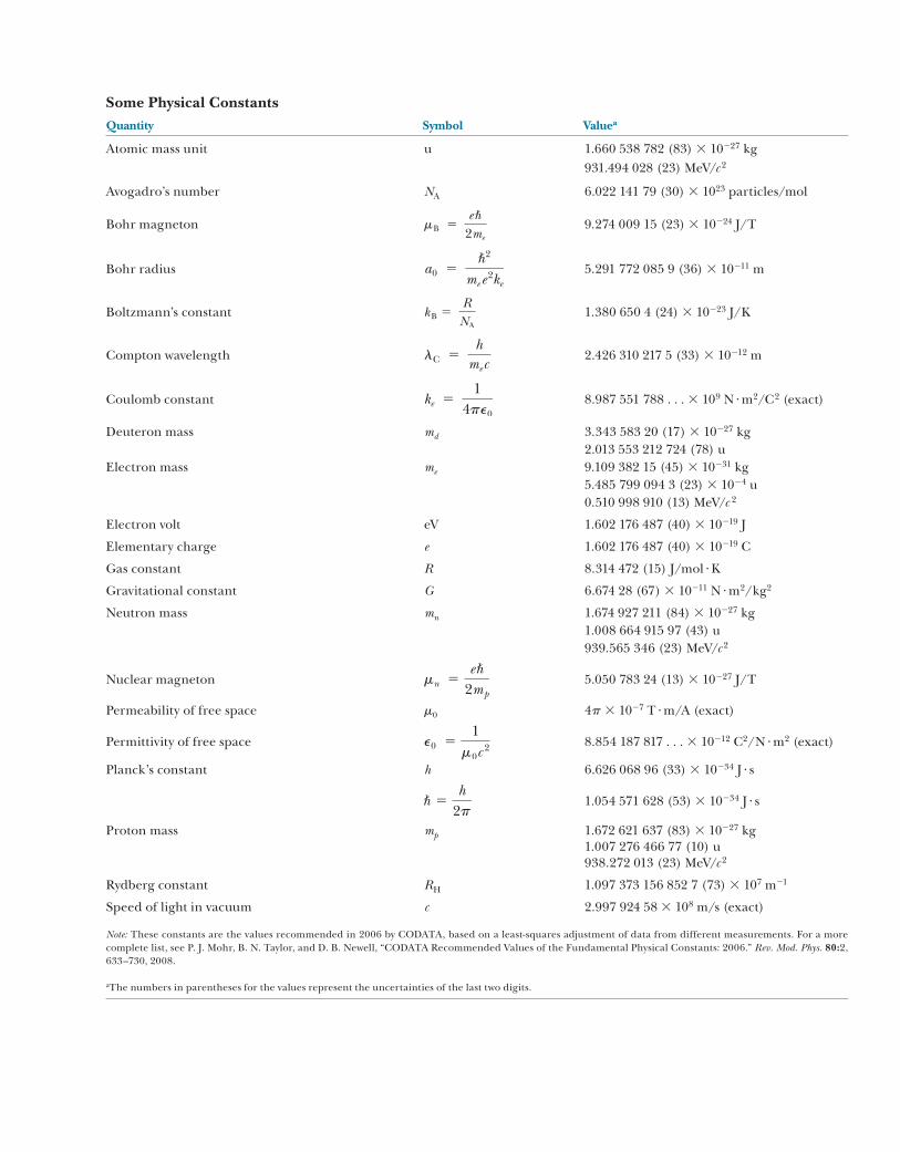
Some Physical ConstantsQuantity Symbol Valuea
Atomic mass unit u 1.660 538 782 (83) 3 10227 kg931.494 028 (23) MeV/c 2
Avogadro’s number NA 6.022 141 79 (30) 3 1023 particles/mol
Bohr magneton mB 5e U
2me9.274 009 15 (23) 3 10224 J/T
Bohr radius a0 5U2
mee2ke
5.291 772 085 9 (36) 3 10211 m
Boltzmann’s constant kB 5RNA
1.380 650 4 (24) 3 10223 J/K
Compton wavelength lC 5h
mec 2.426 310 217 5 (33) 3 10212 m
Coulomb constant ke 51
4pP08.987 551 788 . . . 3 109 N ? m2/C2 (exact)
Deuteron mass md 3.343 583 20 (17) 3 10227 kg2.013 553 212 724 (78) u
Electron mass me 9.109 382 15 (45) 3 10231 kg5.485 799 094 3 (23) 3 1024 u0.510 998 910 (13) MeV/c 2
Electron volt eV 1.602 176 487 (40) 3 10219 J
Elementary charge e 1.602 176 487 (40) 3 10219 C
Gas constant R 8.314 472 (15) J/mol ? K
Gravitational constant G 6.674 28 (67) 3 10211 N ? m2/kg2
Neutron mass mn 1.674 927 211 (84) 3 10227 kg1.008 664 915 97 (43) u939.565 346 (23) MeV/c 2
Nuclear magneton mn 5e U
2mp5.050 783 24 (13) 3 10227 J/T
Permeability of free space m0 4p 3 1027 T ? m/A (exact)
Permittivity of free space P0 51
m0c2 8.854 187 817 . . . 3 10212 C2/N ? m2 (exact)
Planck’s constant h 6.626 068 96 (33) 3 10234 J ? s
U 5h
2p1.054 571 628 (53) 3 10234 J ? s
Proton mass mp 1.672 621 637 (83) 3 10227 kg1.007 276 466 77 (10) u938.272 013 (23) MeV/c 2
Rydberg constant RH 1.097 373 156 852 7 (73) 3 107 m21
Speed of light in vacuum c 2.997 924 58 3 108 m/s (exact)
Note: These constants are the values recommended in 2006 by CODATA, based on a least-squares adjustment of data from different measurements. For a more complete list, see P. J. Mohr, B. N. Taylor, and D. B. Newell, “CODATA Recommended Values of the Fundamental Physical Constants: 2006.” Rev. Mod. Phys. 80:2, 633–730, 2008.
aThe numbers in parentheses for the values represent the uncertainties of the last two digits.
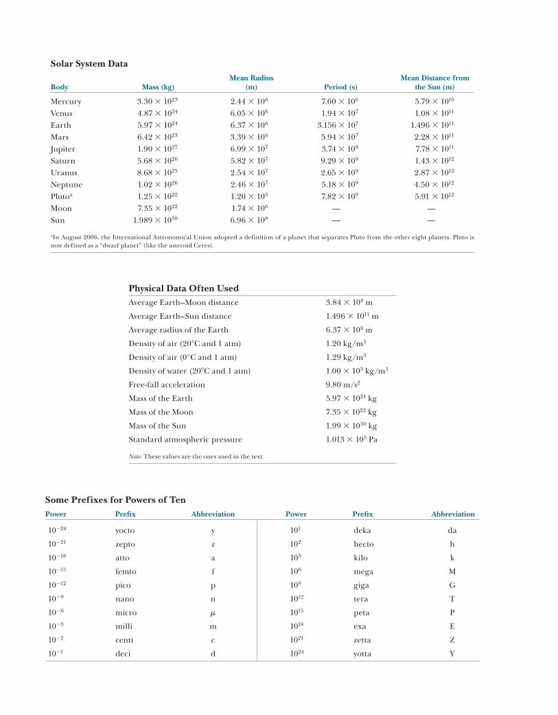
Solar System DataMean Radius Mean Distance from
Body Mass (kg) (m) Period (s) the Sun (m)
Mercury 3.30 3 1023 2.44 3 106 7.60 3 106 5.79 3 1010
Venus 4.87 3 1024 6.05 3 106 1.94 3 107 1.08 3 1011
Earth 5.97 3 1024 6.37 3 106 3.156 3 107 1.496 3 1011
Mars 6.42 3 1023 3.39 3 106 5.94 3 107 2.28 3 1011
Jupiter 1.90 3 1027 6.99 3 107 3.74 3 108 7.78 3 1011
Saturn 5.68 3 1026 5.82 3 107 9.29 3 108 1.43 3 1012
Uranus 8.68 3 1025 2.54 3 107 2.65 3 109 2.87 3 1012
Neptune 1.02 3 1026 2.46 3 107 5.18 3 109 4.50 3 1012
Plutoa 1.25 3 1022 1.20 3 106 7.82 3 109 5.91 3 1012
Moon 7.35 3 1022 1.74 3 106 — —Sun 1.989 3 1030 6.96 3 108 — —
aIn August 2006, the International Astronomical Union adopted a definition of a planet that separates Pluto from the other eight planets. Pluto is now defined as a “dwarf planet” (like the asteroid Ceres).
Physical Data Often UsedAverage Earth–Moon distance 3.84 3 108 m
Average Earth–Sun distance 1.496 3 1011 m
Average radius of the Earth 6.37 3 106 m
Density of air (208C and 1 atm) 1.20 kg/m3
Density of air (0°C and 1 atm) 1.29 kg/m3
Density of water (208C and 1 atm) 1.00 3 103 kg/m3
Free-fall acceleration 9.80 m/s2
Mass of the Earth 5.97 3 1024 kg
Mass of the Moon 7.35 3 1022 kg
Mass of the Sun 1.99 3 1030 kg
Standard atmospheric pressure 1.013 3 105 Pa
Note: These values are the ones used in the text.
Some Prefixes for Powers of TenPower Prefix Abbreviation Power Prefix Abbreviation
10224 yocto y 101 deka da
10221 zepto z 102 hecto h
10218 atto a 103 kilo k
10215 femto f 106 mega M
10212 pico p 109 giga G
1029 nano n 1012 tera T
1026 micro m 1015 peta P
1023 milli m 1018 exa E
1022 centi c 1021 zetta Z
1021 deci d 1024 yotta Y
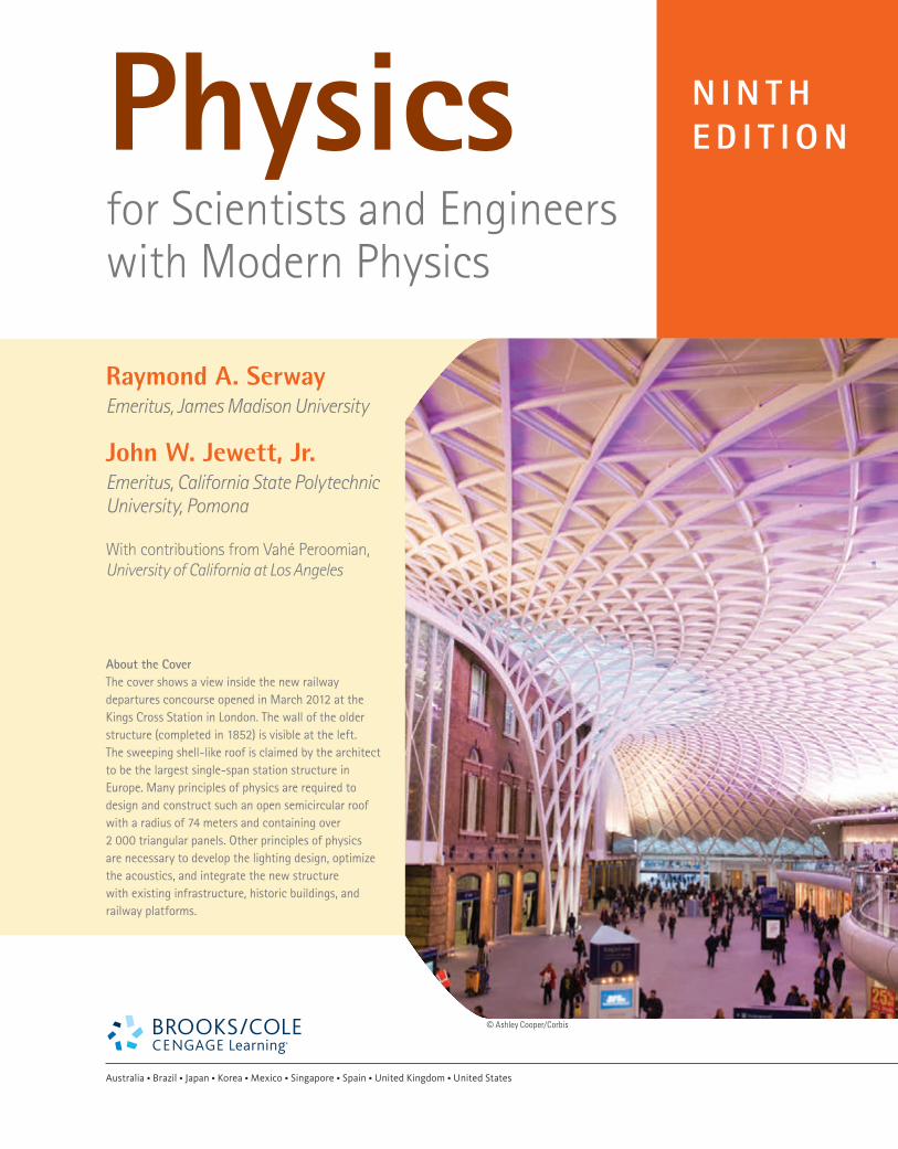
Raymond A. SerwayEmeritus, James Madison University
John W. Jewett, Jr.Emeritus, California State Polytechnic University, Pomona
With contributions from Vahé Peroomian, University of California at Los Angeles
Australia • Brazil • Japan • Korea • Mexico • Singapore • Spain • United Kingdom • United States
N i N t h E d i t i o NPhysics
for Scientists and Engineerswith Modern Physics
© Ashley Cooper/Corbis
About the Cover The cover shows a view inside the new railway departures concourse opened in March 2012 at the Kings Cross Station in London. The wall of the older structure (completed in 1852) is visible at the left. The sweeping shell-like roof is claimed by the architect to be the largest single-span station structure in Europe. Many principles of physics are required to design and construct such an open semicircular roof with a radius of 74 meters and containing over 2 000 triangular panels. Other principles of physics are necessary to develop the lighting design, optimize the acoustics, and integrate the new structure with existing infrastructure, historic buildings, and railway platforms.

2014, 2010, 2008 by Raymond A. Serway
NO RIGHTS RESERVED. Any part of this work may be reproduced, transmitted, stored, or used in any form or by any means graphic, electronic, or mechanical, including but not limited to photocopying, recording, scanning, digitizing, taping, Web distribution, information networks, or information storage and retrieval systems, without the prior written permission of the publisher.
Library of Congress Control Number: 2012947242
ISBN-13: 978-1-133-95405-7
ISBN-10: 1-133-95405-7
Brooks/Cole 20 Channel Center StreetBoston, MA 02210USA
Physics for Scientists and Engineers with Modern Physics, Ninth EditionRaymond A. Serway and John W. Jewett, Jr.
Publisher, Physical Sciences: Mary Finch
Publisher, Physics and Astronomy: Charlie Hartford
Development Editor: Ed Dodd
Assistant Editor: Brandi Kirksey
Editorial Assistant: Brendan Killion
Media Editor: Rebecca Berardy Schwartz
Brand Manager: Nicole Hamm
Marketing Communications Manager: Linda Yip
Senior Marketing Development Manager: Tom Ziolkowski
Content Project Manager: Alison Eigel Zade
Senior Art Director: Cate Barr
Manufacturing Planner: Sandee Milewski
Rights Acquisition Specialist: Shalice Shah-Caldwell
Production Service: Lachina Publishing Services
Text and Cover Designer: Roy Neuhaus
Cover Image: The new Kings Cross railway station, London, UK
Cover Image Credit: © Ashley Cooper/Corbis
Compositor: Lachina Publishing Services
Printed in the United States of America 1 2 3 4 5 6 7 16 15 14 13 12
We dedicate this book to our wives, Elizabeth and Lisa, and all our children and grandchildren for their loving understanding
when we spent time on writing instead of being with them.
iii
Brief Contents
p a r T 1Mechanics 1
1 Physics and Measurement 2
2 Motion in One Dimension 21
3 Vectors 59
4 Motion in Two Dimensions 78
5 The Laws of Motion 111
6 Circular Motion and Other Applicationsof Newton’s Laws 150
7 Energy of a System 177
8 Conservation of Energy 211
9 Linear Momentum and Collisions 247
10 Rotation of a Rigid Object Abouta Fixed Axis 293
11 Angular Momentum 335
12 Static Equilibrium and Elasticity 363
13 Universal Gravitation 388
14 Fluid Mechanics 417
p a r T 2Oscillations and Mechanical Waves 449 15 Oscillatory Motion 450
16 Wave Motion 483
17 Sound Waves 507
18 Superposition and Standing Waves 533
p a r T 3Thermodynamics 567 19 Temperature 568
20 The First Law of Thermodynamics 590
21 The Kinetic Theory of Gases 626
22 Heat Engines, Entropy, and the Second Lawof Thermodynamics 653
p a r T 4Electricity and Magnetism 689 23 Electric Fields 690
24 Gauss’s Law 725
25 Electric Potential 746
26 Capacitance and Dielectrics 777
27 Current and Resistance 808
28 Direct-Current Circuits 833
29 Magnetic Fields 868
30 Sources of the Magnetic Field 904
31 Faraday’s Law 935
32 Inductance 970
33 Alternating-Current Circuits 998
34 Electromagnetic Waves 1030
p a r T 5Light and Optics 1057 35 The Nature of Light and the Principles
of Ray Optics 1058
36 Image Formation 1090
37 Wave Optics 1134
38 Diffraction Patterns and Polarization 1160
p a r T 6Modern Physics 1191 39 Relativity 1192
40 Introduction to Quantum Physics 1233
41 Quantum Mechanics 1267
42 Atomic Physics 1296
43 Molecules and Solids 1340
44 Nuclear Structure 1380
45 Applications of Nuclear Physics 1418
46 Particle Physics and Cosmology 1447

iv
About the Authors viii
Preface ix
To the Student xxx
p a r T 1Mechanics 1 1 Physics and Measurement 2
1.1 Standards of Length, Mass, and Time 31.2 Matter and Model Building 61.3 Dimensional Analysis 71.4 Conversion of Units 91.5 Estimates and Order-of-Magnitude Calculations 101.6 Significant Figures 11
2 Motion in One Dimension 212.1 Position, Velocity, and Speed 222.2 Instantaneous Velocity and Speed 252.3 Analysis Model: Particle Under Constant Velocity 282.4 Acceleration 312.5 Motion Diagrams 352.6 Analysis Model: Particle Under Constant Acceleration 362.7 Freely Falling Objects 402.8 Kinematic Equations Derived from Calculus 43
3 Vectors 593.1 Coordinate Systems 593.2 Vector and Scalar Quantities 613.3 Some Properties of Vectors 623.4 Components of a Vector and Unit Vectors 65
4 Motion in Two Dimensions 784.1 The Position, Velocity, and Acceleration Vectors 784.2 Two-Dimensional Motion with Constant Acceleration 814.3 Projectile Motion 844.4 Analysis Model: Particle in Uniform Circular Motion 914.5 Tangential and Radial Acceleration 944.6 Relative Velocity and Relative Acceleration 96
5 The Laws of Motion 1115.1 The Concept of Force 1115.2 Newton’s First Law and Inertial Frames 1135.3 Mass 1145.4 Newton’s Second Law 1155.5 The Gravitational Force and Weight 1175.6 Newton’s Third Law 1185.7 Analysis Models Using Newton’s Second Law 1205.8 Forces of Friction 130
6 Circular Motion and Other Applications of Newton’s Laws 150
6.1 Extending the Particle in Uniform Circular Motion Model 1506.2 Nonuniform Circular Motion 1566.3 Motion in Accelerated Frames 1586.4 Motion in the Presence of Resistive Forces 161
7 Energy of a System 1777.1 Systems and Environments 1787.2 Work Done by a Constant Force 1787.3 The Scalar Product of Two Vectors 1817.4 Work Done by a Varying Force 1837.5 Kinetic Energy and the Work–Kinetic Energy Theorem 1887.6 Potential Energy of a System 1917.7 Conservative and Nonconservative Forces 1967.8 Relationship Between Conservative Forces
and Potential Energy 1987.9 Energy Diagrams and Equilibrium of a System 199
8 Conservation of Energy 2118.1 Analysis Model: Nonisolated System (Energy) 2128.2 Analysis Model: Isolated System (Energy) 2158.3 Situations Involving Kinetic Friction 2228.4 Changes in Mechanical Energy for Nonconservative Forces 2278.5 Power 232
9 Linear Momentum and Collisions 2479.1 Linear Momentum 2479.2 Analysis Model: Isolated System (Momentum) 2509.3 Analysis Model: Nonisolated System (Momentum) 2529.4 Collisions in One Dimension 2569.5 Collisions in Two Dimensions 2649.6 The Center of Mass 2679.7 Systems of Many Particles 2729.8 Deformable Systems 2759.9 Rocket Propulsion 277
10 Rotation of a Rigid Object About a Fixed Axis 293
10.1 Angular Position, Velocity, and Acceleration 29310.2 Analysis Model: Rigid Object Under Constant
Angular Acceleration 29610.3 Angular and Translational Quantities 298
10.4 Torque 30010.5 Analysis Model: Rigid Object Under a Net Torque 30210.6 Calculation of Moments of Inertia 30710.7 Rotational Kinetic Energy 31110.8 Energy Considerations in Rotational Motion 31210.9 Rolling Motion of a Rigid Object 316
11 Angular Momentum 33511.1 The Vector Product and Torque 33511.2 Analysis Model: Nonisolated System (Angular Momentum) 338
Contents
Contents v
11.3 Angular Momentum of a Rotating Rigid Object 34211.4 Analysis Model: Isolated System (Angular Momentum) 34511.5 The Motion of Gyroscopes and Tops 350
12 Static Equilibrium and Elasticity 36312.1 Analysis Model: Rigid Object in Equilibrium 36312.2 More on the Center of Gravity 36512.3 Examples of Rigid Objects in Static Equilibrium 36612.4 Elastic Properties of Solids 373
13 Universal Gravitation 38813.1 Newton’s Law of Universal Gravitation 38913.2 Free-Fall Acceleration and the Gravitational Force 39113.3 Analysis Model: Particle in a Field (Gravitational) 39213.4 Kepler’s Laws and the Motion of Planets 39413.5 Gravitational Potential Energy 40013.6 Energy Considerations in Planetary and Satellite Motion 402
14 Fluid Mechanics 417 14.1 Pressure 417
14.2 Variation of Pressure with Depth 41914.3 Pressure Measurements 42314.4 Buoyant Forces and Archimedes’s Principle 42314.5 Fluid Dynamics 42714.6 Bernoulli’s Equation 43014.7 Other Applications of Fluid Dynamics 433
p a r T 2Oscillations and Mechanical Waves 449 15 Oscillatory Motion 450
15.1 Motion of an Object Attached to a Spring 45015.2 Analysis Model: Particle in Simple Harmonic Motion 45215.3 Energy of the Simple Harmonic Oscillator 45815.4 Comparing Simple Harmonic Motion with Uniform
Circular Motion 46215.5 The Pendulum 46415.6 Damped Oscillations 46815.7 Forced Oscillations 469
16 Wave Motion 48316.1 Propagation of a Disturbance 48416.2 Analysis Model: Traveling Wave 48716.3 The Speed of Waves on Strings 49116.4 Reflection and Transmission 49416.5 Rate of Energy Transfer by Sinusoidal Waves on Strings 49516.6 The Linear Wave Equation 497
17 Sound Waves 50717.1 Pressure Variations in Sound Waves 50817.2 Speed of Sound Waves 51017.3 Intensity of Periodic Sound Waves 51217.4 The Doppler Effect 517
18 Superposition and Standing Waves 53318.1 Analysis Model: Waves in Interference 53418.2 Standing Waves 53818.3 Analysis Model: Waves Under Boundary Conditions 541
18.4 Resonance 54618.5 Standing Waves in Air Columns 54618.6 Standing Waves in Rods and Membranes 55018.7 Beats: Interference in Time 55018.8 Nonsinusoidal Wave Patterns 553
p a r T 3Thermodynamics 567 19 Temperature 568
19.1 Temperature and the Zeroth Law of Thermodynamics 56819.2 Thermometers and the Celsius Temperature Scale 57019.3 The Constant-Volume Gas Thermometer and the Absolute
Temperature Scale 57119.4 Thermal Expansion of Solids and Liquids 57319.5 Macroscopic Description of an Ideal Gas 578
20 The First Law of Thermodynamics 59020.1 Heat and Internal Energy 59020.2 Specific Heat and Calorimetry 59320.3 Latent Heat 59720.4 Work and Heat in Thermodynamic Processes 60120.5 The First Law of Thermodynamics 60320.6 Some Applications of the First Law of Thermodynamics 60420.7 Energy Transfer Mechanisms in Thermal Processes 608
21 The Kinetic Theory of Gases 62621.1 Molecular Model of an Ideal Gas 62721.2 Molar Specific Heat of an Ideal Gas 63121.3 The Equipartition of Energy 63521.4 Adiabatic Processes for an Ideal Gas 63721.5 Distribution of Molecular Speeds 639
22 Heat Engines, Entropy, and the Second Law of Thermodynamics 653
22.1 Heat Engines and the Second Law of Thermodynamics 65422.2 Heat Pumps and Refrigerators 65622.3 Reversible and Irreversible Processes 65922.4 The Carnot Engine 66022.5 Gasoline and Diesel Engines 665
22.6 Entropy 66722.7 Changes in Entropy for Thermodynamic Systems 67122.8 Entropy and the Second Law 676
p a r T 4Electricity and Magnetism 689 23 Electric Fields 690
23.1 Properties of Electric Charges 69023.2 Charging Objects by Induction 69223.3 Coulomb’s Law 69423.4 Analysis Model: Particle in a Field (Electric) 69923.5 Electric Field of a Continuous Charge Distribution 70423.6 Electric Field Lines 70823.7 Motion of a Charged Particle in a Uniform Electric Field 710
24 Gauss’s Law 72524.1 Electric Flux 72524.2 Gauss’s Law 72824.3 Application of Gauss’s Law to Various Charge Distributions 73124.4 Conductors in Electrostatic Equilibrium 735
25 Electric Potential 74625.1 Electric Potential and Potential Difference 74625.2 Potential Difference in a Uniform Electric Field 748

vi Contents
25.3 Electric Potential and Potential Energy Due to Point Charges 752
25.4 Obtaining the Value of the Electric Field from the Electric Potential 755
25.5 Electric Potential Due to Continuous Charge Distributions 75625.6 Electric Potential Due to a Charged Conductor 76125.7 The Millikan Oil-Drop Experiment 76425.8 Applications of Electrostatics 765
26 Capacitance and Dielectrics 77726.1 Definition of Capacitance 77726.2 Calculating Capacitance 77926.3 Combinations of Capacitors 78226.4 Energy Stored in a Charged Capacitor 78626.5 Capacitors with Dielectrics 79026.6 Electric Dipole in an Electric Field 79326.7 An Atomic Description of Dielectrics 795
27 Current and Resistance 80827.1 Electric Current 808
27.2 Resistance 81127.3 A Model for Electrical Conduction 81627.4 Resistance and Temperature 819
27.5 Superconductors 81927.6 Electrical Power 820
28 Direct-Current Circuits 83328.1 Electromotive Force 83328.2 Resistors in Series and Parallel 83628.3 Kirchhoff’s Rules 843
28.4 RC Circuits 84628.5 Household Wiring and Electrical Safety 852
29 Magnetic Fields 86829.1 Analysis Model: Particle in a Field (Magnetic) 86929.2 Motion of a Charged Particle in a Uniform Magnetic Field 87429.3 Applications Involving Charged Particles Moving
in a Magnetic Field 87929.4 Magnetic Force Acting on a Current-Carrying Conductor 88229.5 Torque on a Current Loop in a Uniform Magnetic Field 88529.6 The Hall Effect 890
30 Sources of the Magnetic Field 90430.1 The Biot–Savart Law 90430.2 The Magnetic Force Between Two Parallel Conductors 90930.3 Ampère’s Law 91130.4 The Magnetic Field of a Solenoid 91530.5 Gauss’s Law in Magnetism 91630.6 Magnetism in Matter 919
31 Faraday’s Law 93531.1 Faraday’s Law of Induction 93531.2 Motional emf 93931.3 Lenz’s Law 94431.4 Induced emf and Electric Fields 94731.5 Generators and Motors 94931.6 Eddy Currents 953
32 Inductance 97032.1 Self-Induction and Inductance 970
32.2 RL Circuits 97232.3 Energy in a Magnetic Field 97632.4 Mutual Inductance 97832.5 Oscillations in an LC Circuit 980
32.6 The RLC Circuit 984
33 Alternating-Current Circuits 99833.1 AC Sources 99833.2 Resistors in an AC Circuit 99933.3 Inductors in an AC Circuit 100233.4 Capacitors in an AC Circuit 1004
33.5 The RLC Series Circuit 100733.6 Power in an AC Circuit 101133.7 Resonance in a Series RLC Circuit 101333.8 The Transformer and Power Transmission 101533.9 Rectifiers and Filters 1018
34 Electromagnetic Waves 103034.1 Displacement Current and the General Form of Ampère’s Law 103134.2 Maxwell’s Equations and Hertz’s Discoveries 103334.3 Plane Electromagnetic Waves 103534.4 Energy Carried by Electromagnetic Waves 103934.5 Momentum and Radiation Pressure 104234.6 Production of Electromagnetic Waves by an Antenna 104434.7 The Spectrum of Electromagnetic Waves 1045
p a r T 5Light and Optics 1057 35 The Nature of Light and the Principles
of Ray Optics 105835.1 The Nature of Light 105835.2 Measurements of the Speed of Light 105935.3 The Ray Approximation in Ray Optics 106135.4 Analysis Model: Wave Under Reflection 106135.5 Analysis Model: Wave Under Refraction 106535.6 Huygens’s Principle 1071
35.7 Dispersion 107235.8 Total Internal Reflection 1074
36 Image Formation 109036.1 Images Formed by Flat Mirrors 109036.2 Images Formed by Spherical Mirrors 109336.3 Images Formed by Refraction 110036.4 Images Formed by Thin Lenses 110436.5 Lens Aberrations 111236.6 The Camera 111336.7 The Eye 111536.8 The Simple Magnifier 111836.9 The Compound Microscope 1119
36.10 The Telescope 1120
37 Wave Optics 113437.1 Young’s Double-Slit Experiment 113437.2 Analysis Model: Waves in Interference 113737.3 Intensity Distribution of the Double-Slit Interference Pattern 114037.4 Change of Phase Due to Reflection 114337.5 Interference in Thin Films 114437.6 The Michelson Interferometer 1147
38 Diffraction Patterns and Polarization 116038.1 Introduction to Diffraction Patterns 116038.2 Diffraction Patterns from Narrow Slits 116138.3 Resolution of Single-Slit and Circular Apertures 116638.4 The Diffraction Grating 116938.5 Diffraction of X-Rays by Crystals 117438.6 Polarization of Light Waves 1175

Contents vii
44.5 The Decay Processes 1394 44.6 Natural Radioactivity 1404 44.7 Nuclear Reactions 1405 44.8 Nuclear Magnetic Resonance and Magnetic
Resonance Imaging 1406
45 Applications of Nuclear Physics 1418 45.1 Interactions Involving Neutrons 1418 45.2 Nuclear Fission 1419 45.3 Nuclear Reactors 1421 45.4 Nuclear Fusion 1425 45.5 Radiation Damage 1432 45.6 Uses of Radiation 1434
46 Particle Physics and Cosmology 1447 46.1 The Fundamental Forces in Nature 1448 46.2 Positrons and Other Antiparticles 1449 46.3 Mesons and the Beginning of Particle Physics 1451 46.4 Classification of Particles 1454 46.5 Conservation Laws 1455 46.6 Strange Particles and Strangeness 1459 46.7 Finding Patterns in the Particles 1460 46.8 Quarks 1462 46.9 Multicolored Quarks 1465 46.10 The Standard Model 1467 46.11 The Cosmic Connection 1469 46.12 Problems and Perspectives 1474
Appendices A Tables A-1 A.1 Conversion Factors A-1 A.2 Symbols, Dimensions, and Units of Physical Quantities A-2
B Mathematics Review A-4 B.1 Scientific Notation A-4 B.2 Algebra A-5 B.3 Geometry A-10 B.4 Trigonometry A-11 B.5 Series Expansions A-13 B.6 Differential Calculus A-13 B.7 Integral Calculus A-16 B.8 Propagation of Uncertainty A-20
C Periodic Table of the Elements A-22
D SI Units A-24 D.1 SI Units A-24 D.2 Some Derived SI Units A-24
Answers to Quick Quizzes and Odd-Numbered Problems A-25
Index I-1
p a r T 6Modern Physics 1191 39 Relativity 1192 39.1 The Principle of Galilean Relativity 1193 39.2 The Michelson–Morley Experiment 1196 39.3 Einstein’s Principle of Relativity 1198 39.4 Consequences of the Special Theory of Relativity 1199 39.5 The Lorentz Transformation Equations 1210 39.6 The Lorentz Velocity Transformation Equations 1212 39.7 Relativistic Linear Momentum 1214 39.8 Relativistic Energy 1216 39.9 The General Theory of Relativity 1220
40 Introduction to Quantum Physics 1233 40.1 Blackbody Radiation and Planck’s Hypothesis 1234 40.2 The Photoelectric Effect 1240 40.3 The Compton Effect 1246 40.4 The Nature of Electromagnetic Waves 1249 40.5 The Wave Properties of Particles 1249 40.6 A New Model: The Quantum Particle 1252 40.7 The Double-Slit Experiment Revisited 1255 40.8 The Uncertainty Principle 1256
41 Quantum Mechanics 1267 41.1 The Wave Function 1267 41.2 Analysis Model: Quantum Particle Under
Boundary Conditions 1271 41.3 The Schrödinger Equation 1277 41.4 A Particle in a Well of Finite Height 1279 41.5 Tunneling Through a Potential Energy Barrier 1281 41.6 Applications of Tunneling 1282 41.7 The Simple Harmonic Oscillator 1286
42 Atomic Physics 1296 42.1 Atomic Spectra of Gases 1297 42.2 Early Models of the Atom 1299 42.3 Bohr’s Model of the Hydrogen Atom 1300 42.4 The Quantum Model of the Hydrogen Atom 1306 42.5 The Wave Functions for Hydrogen 1308 42.6 Physical Interpretation of the Quantum Numbers 1311 42.7 The Exclusion Principle and the Periodic Table 1318 42.8 More on Atomic Spectra: Visible and X-Ray 1322 42.9 Spontaneous and Stimulated Transitions 1325 42.10 Lasers 1326
43 Molecules and Solids 1340 43.1 Molecular Bonds 1341 43.2 Energy States and Spectra of Molecules 1344 43.3 Bonding in Solids 1352 43.4 Free-Electron Theory of Metals 1355 43.5 Band Theory of Solids 1359 43.6 Electrical Conduction in Metals, Insulators,
and Semiconductors 1361 43.7 Semiconductor Devices 1364 43.8 Superconductivity 1370
44 Nuclear Structure 1380 44.1 Some Properties of Nuclei 1381 44.2 Nuclear Binding Energy 1386 44.3 Nuclear Models 1387 44.4 Radioactivity 1390

viii
About the Authors
Raymond A. Serway received his doctorate at Illinois Institute of Technol-ogy and is Professor Emeritus at James Madison University. In 2011, he was awarded with an honorary doctorate degree from his alma mater, Utica College. He received the 1990 Madison Scholar Award at James Madison University, where he taught for 17 years. Dr. Serway began his teaching career at Clarkson University, where he con-ducted research and taught from 1967 to 1980. He was the recipient of the Distin-guished Teaching Award at Clarkson University in 1977 and the Alumni Achievement Award from Utica College in 1985. As Guest Scientist at the IBM Research Laboratory in Zurich, Switzerland, he worked with K. Alex Müller, 1987 Nobel Prize recipient. Dr. Serway also was a visiting scientist at Argonne National Laboratory, where he col-laborated with his mentor and friend, the late Dr. Sam Marshall. Dr. Serway is the coauthor of College Physics, Ninth Edition; Principles of Physics, Fifth Edition; Essentials of College Physics; Modern Physics, Third Edition; and the high school textbook Physics,
published by Holt McDougal. In addition, Dr. Serway has published more than 40 research papers in the field of con-densed matter physics and has given more than 60 presentations at professional meetings. Dr. Serway and his wife, Eliza-beth, enjoy traveling, playing golf, fishing, gardening, singing in the church choir, and especially spending quality time with their four children, ten grandchildren, and a recent great grandson.
John W. Jewett, Jr. earned his undergraduate degree in physics at DrexelUniversity and his doctorate at Ohio State University, specializing in optical and magnetic properties of condensed matter. Dr. Jewett began his academic career at Richard Stockton College of New Jersey, where he taught from 1974 to 1984. He is currently Emeritus Professor of Physics at California State Polytechnic University, Pomona. Through his teaching career, Dr. Jewett has been active in promoting effec-tive physics education. In addition to receiving four National Science Foundation grants in physics education, he helped found and direct the Southern California Area Modern Physics Institute (SCAMPI) and Science IMPACT (Institute for Mod-ern Pedagogy and Creative Teaching). Dr. Jewett’s honors include the Stockton Merit Award at Richard Stockton College in 1980, selection as Outstanding Professor at California State Polytechnic University for 1991–1992, and the Excellence in Under-graduate Physics Teaching Award from the American Association of Physics Teachers
(AAPT) in 1998. In 2010, he received an Alumni Lifetime Achievement Award from Drexel University in recognition of his contributions in physics education. He has given more than 100 presentations both domestically and abroad, includ-ing multiple presentations at national meetings of the AAPT. He has also published 25 research papers in condensed matter physics and physics education research. Dr. Jewett is the author of The World of Physics: Mysteries, Magic, and Myth, which provides many connections between physics and everyday experiences. In addition to his work as the coauthor for Physics for Scientists and Engineers, he is also the coauthor on Principles of Physics, Fifth Edition, as well as Global Issues, a four-volume set of instruction manuals in integrated science for high school. Dr. Jewett enjoys playing keyboard with his all-physicist band, traveling, underwater photography, learning foreign languages, and collecting antique quack medical devices that can be used as demonstration apparatus in physics lectures. Most importantly, he relishes spending time with his wife, Lisa, and their children and grandchildren.

ix
Preface
In writing this Ninth Edition of Physics for Scientists and Engineers, we continue our ongoing efforts to improve the clarity of presentation and include new pedagogical features that help support the learning and teaching processes. Drawing on positive feedback from users of the Eighth Edition, data gathered from both professors and students who use Enhanced WebAssign, as well as reviewers’ suggestions, we have refined the text to better meet the needs of students and teachers. This textbook is intended for a course in introductory physics for students majoring in science or engineering. The entire contents of the book in its extended version could be covered in a three-semester course, but it is pos-sible to use the material in shorter sequences with the omission of selected chapters and sections. The mathematical background of the student taking this course should ideally include one semester of calculus. If that is not possible, the student should be enrolled in a concurrent course in introductory calculus.
ContentThe material in this book covers fundamental topics in classical physics and provides an introduction to modern phys-ics. The book is divided into six parts. Part 1 (Chapters 1 to 14) deals with the fundamentals of Newtonian mechanics and the physics of fluids; Part 2 (Chapters 15 to 18) covers oscillations, mechanical waves, and sound; Part 3 (Chap-ters 19 to 22) addresses heat and thermodynamics; Part 4 (Chapters 23 to 34) treats electricity and magnetism; Part 5 (Chapters 35 to 38) covers light and optics; and Part 6 (Chapters 39 to 46) deals with relativity and modern physics.
ObjectivesThis introductory physics textbook has three main objectives: to provide the student with a clear and logical presen-tation of the basic concepts and principles of physics, to strengthen an understanding of the concepts and principles through a broad range of interesting real-world applications, and to develop strong problem-solving skills through an effectively organized approach. To meet these objectives, we emphasize well-organized physical arguments and a focused problem-solving strategy. At the same time, we attempt to motivate the student through practical examples that demonstrate the role of physics in other disciplines, including engineering, chemistry, and medicine.
Changes in the Ninth EditionA large number of changes and improvements were made for the Ninth Edition of this text. Some of the new fea-tures are based on our experiences and on current trends in science education. Other changes were incorporated in response to comments and suggestions offered by users of the Eighth Edition and by reviewers of the manuscript. The features listed here represent the major changes in the Ninth Edition.
Enhanced Integration of the Analysis Model Approach to Problem Solving. Students are faced with hundreds of problems during their physics courses. A relatively small number of fundamental principles form the basis of these problems. When faced with a new problem, a physicist forms a model of the problem that can be solved in a simple way by iden-tifying the fundamental principle that is applicable in the problem. For example, many problems involve conserva-tion of energy, Newton’s second law, or kinematic equations. Because the physicist has studied these principles and their applications extensively, he or she can apply this knowledge as a model for solving a new problem. Although it would be ideal for students to follow this same process, most students have difficulty becoming familiar with the entire palette of fundamental principles that are available. It is easier for students to identify a situation rather than a fundamental principle.
x Preface
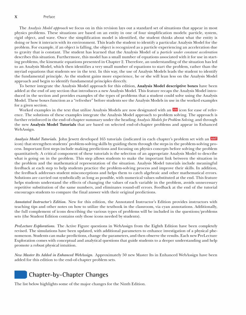
The Analysis Model approach we focus on in this revision lays out a standard set of situations that appear in most physics problems. These situations are based on an entity in one of four simplification models: particle, system, rigid object, and wave. Once the simplification model is identified, the student thinks about what the entity is doing or how it interacts with its environment. This leads the student to identify a particular Analysis Model for the problem. For example, if an object is falling, the object is recognized as a particle experiencing an acceleration due to gravity that is constant. The student has learned that the Analysis Model of a particle under constant acceleration describes this situation. Furthermore, this model has a small number of equations associated with it for use in start-ing problems, the kinematic equations presented in Chapter 2. Therefore, an understanding of the situation has led to an Analysis Model, which then identifies a very small number of equations to start the problem, rather than the myriad equations that students see in the text. In this way, the use of Analysis Models leads the student to identify the fundamental principle. As the student gains more experience, he or she will lean less on the Analysis Model approach and begin to identify fundamental principles directly. To better integrate the Analysis Model approach for this edition, Analysis Model descriptive boxes have been added at the end of any section that introduces a new Analysis Model. This feature recaps the Analysis Model intro-duced in the section and provides examples of the types of problems that a student could solve using the Analysis Model. These boxes function as a “refresher” before students see the Analysis Models in use in the worked examples for a given section. Worked examples in the text that utilize Analysis Models are now designated with an AM icon for ease of refer-ence. The solutions of these examples integrate the Analysis Model approach to problem solving. The approach is further reinforced in the end-of-chapter summary under the heading Analysis Models for Problem Solving, and through the new Analysis Model Tutorials that are based on selected end-of-chapter problems and appear in Enhanced WebAssign.
Analysis Model Tutorials. John Jewett developed 165 tutorials (indicated in each chapter’s problem set with an AMT icon) that strengthen students’ problem-solving skills by guiding them through the steps in the problem-solving pro-cess. Important first steps include making predictions and focusing on physics concepts before solving the problem quantitatively. A critical component of these tutorials is the selection of an appropriate Analysis Model to describe what is going on in the problem. This step allows students to make the important link between the situation in the problem and the mathematical representation of the situation. Analysis Model tutorials include meaningful feedback at each step to help students practice the problem-solving process and improve their skills. In addition, the feedback addresses student misconceptions and helps them to catch algebraic and other mathematical errors. Solutions are carried out symbolically as long as possible, with numerical values substituted at the end. This feature helps students understand the effects of changing the values of each variable in the problem, avoids unnecessary repetitive substitution of the same numbers, and eliminates round-off errors. Feedback at the end of the tutorial encourages students to compare the final answer with their original predictions.
Annotated Instructor’s Edition. New for this edition, the Annotated Instructor’s Edition provides instructors with teaching tips and other notes on how to utilize the textbook in the classroom, via cyan annotations. Additionally, the full complement of icons describing the various types of problems will be included in the questions/problems sets (the Student Edition contains only those icons needed by students).
PreLecture Explorations. The Active Figure questions in WebAssign from the Eighth Edition have been completely revised. The simulations have been updated, with additional parameters to enhance investigation of a physical phe-nomenon. Students can make predictions, change the parameters, and then observe the results. Each new PreLecture Exploration comes with conceptual and analytical questions that guide students to a deeper understanding and help promote a robust physical intuition.
New Master Its Added in Enhanced WebAssign. Approximately 50 new Master Its in Enhanced WebAssign have been added for this edition to the end-of-chapter problem sets.
Chapter-by-Chapter ChangesThe list below highlights some of the major changes for the Ninth Edition.

Preface xi
Chapter 1• Two new Master Its were added to the end-of-chapter
problems set.• Three new Analysis Model Tutorials were added for this
chapter in Enhanced WebAssign.
Chapter 2• A new introduction to the concept of Analysis Models
has been included in Section 2.3.• Three Analysis Model descriptive boxes have been
added, in Sections 2.3 and 2.6.• Several textual sections have been revised to make more
explicit references to analysis models.• Three new Master Its were added to the end-of-chapter
problems set.• Five new Analysis Model Tutorials were added for this
chapter in Enhanced WebAssign.
Chapter 3• Three new Analysis Model Tutorials were added for this
chapter in Enhanced WebAssign.
Chapter 4• An Analysis Model descriptive box has been added, in
Section 4.6.• Several textual sections have been revised to make more
explicit references to analysis models.• Three new Master Its were added to the end-of-chapter
problems set.• Five new Analysis Model Tutorials were added for this
chapter in Enhanced WebAssign.
Chapter 5• Two Analysis Model descriptive boxes have been added,
in Section 5.7.• Several examples have been modified so that numerical
values are put in only at the end of the solution.• Several textual sections have been revised to make more
explicit references to analysis models.• Four new Master Its were added to the end-of-chapter
problems set.• Four new Analysis Model Tutorials were added for this
chapter in Enhanced WebAssign.
Chapter 6• An Analysis Model descriptive box has been added, in
Section 6.1.• Several examples have been modified so that numerical
values are put in only at the end of the solution.• Four new Analysis Model Tutorials were added for this
chapter in Enhanced WebAssign.
Chapter 7• The notation for work done on a system externally and
internally within a system has been clarified.• The equations and discussions in several sections have
been modified to more clearly show the comparisons of similar potential energy equations among different situations.
• One new Master It was added to the end-of-chapterproblems set.
• Four new Analysis Model Tutorials were added for thischapter in Enhanced WebAssign.
Chapter 8• Two Analysis Model descriptive boxes have been added,
in Sections 8.1 and 8.2.• The problem-solving strategy in Section 8.2 has been
reworded to account for a more general application to both isolated and nonisolated systems.
• As a result of a suggestion from a PER team at Univer-sity of Washington and Pennsylvania State University, Example 8.1 has been rewritten to demonstrate to students the effect of choosing different systems on the development of the solution.
• All examples in the chapter have been rewritten tobegin with Equation 8.2 directly rather than beginning with the format Ei 5 Ef .
• Several examples have been modified so that numericalvalues are put in only at the end of the solution.
• The problem-solving strategy in Section 8.4 has beendeleted and the text material revised to incorporate these ideas on handling energy changes when noncon-servative forces act.
• Several textual sections have been revised to make moreexplicit references to analysis models.
• One new Master It was added to the end-of-chapterproblems set.
• Four new Analysis Model Tutorials were added for thischapter in Enhanced WebAssign.
Chapter 9• Two Analysis Model descriptive boxes have been added,
in Section 9.3.• Several examples have been modified so that numerical
values are put in only at the end of the solution.• Five new Master Its were added to the end-of-chapter
problems set.• Four new Analysis Model Tutorials were added for this
chapter in Enhanced WebAssign.
Chapter 10• The order of four sections (10.4–10.7) has been modified
so as to introduce moment of inertia through torque (rather than energy) and to place the two sections on energy together. The sections have been revised accord-ingly to account for the revised development of con-cepts. This revision makes the order of approach similar to the order of approach students have already seen in translational motion.
• New introductory paragraphs have been added to sev-eral sections to show how the development of our analy-sis of rotational motion parallels that followed earlier for translational motion.
• Two Analysis Model descriptive boxes have been added,in Sections 10.2 and 10.5.
• Several textual sections have been revised to make moreexplicit references to analysis models.

xii Preface
• Two new Master Its were added to the end-of-chapterproblems set.
• Four new Analysis Model Tutorials were added for thischapter in Enhanced WebAssign.
Chapter 11• Two Analysis Model descriptive boxes have been added,
in Sections 11.2 and 11.4.• Angular momentum conservation equations have been
revised so as to be presented as DL 5 (0 or tdt) in order to be consistent with the approach in Chapter 8 for energy conservation and Chapter 9 for linear momen-tum conservation.
• Four new Analysis Model Tutorials were added for thischapter in Enhanced WebAssign.
Chapter 12• One Analysis Model descriptive box has been added, in
Section 12.1.• Several examples have been modified so that numerical
values are put in only at the end of the solution.• Four new Analysis Model Tutorials were added for this
chapter in Enhanced WebAssign.
Chapter 13• Sections 13.3 and 13.4 have been interchanged to pro-
vide a better flow of concepts.• A new analysis model has been introduced: Particle in a
Field (Gravitational). This model is introduced because it represents a physical situation that occurs often. In addition, the model is introduced to anticipate the importance of versions of this model later in electric-ity and magnetism, where it is even more critical. An Analysis Model descriptive box has been added in Section 13.3. In addition, a new summary flash card has been added at the end of the chapter, and textual material has been revised to make reference to the new model.
• The description of the historical goals of the Cavendishexperiment in 1798 has been revised to be more consis-tent with Cavendish’s original intent and the knowledge available at the time of the experiment.
• Newly discovered Kuiper belt objects have been added,in Section 13.4.
• Textual material has been modified to make a strongertie-in to Analysis Models, especially in the energy sec-tions 13.5 and 13.6.
• All conservation equations have been revised so as to bepresented with the change in the system on the left and the transfer across the boundary of the system on the right, in order to be consistent with the approach in ear-lier chapters for energy conservation, linear momentum conservation, and angular momentum conservation.
• Four new Analysis Model Tutorials were added for thischapter in Enhanced WebAssign.
Chapter 14• Several textual sections have been revised to make more
explicit references to Analysis Models.• Several examples have been modified so that numerical
values are put in only at the end of the solution.
• One new Master It was added to the end-of-chapterproblems set.
• Four new Analysis Model Tutorials were added for thischapter in Enhanced WebAssign.
Chapter 15• An Analysis Model descriptive box has been added, in
Section 15.2.• Several textual sections have been revised to make more
explicit references to Analysis Models.• Four new Master Its were added to the end-of-chapter
problems set.• Four new Analysis Model Tutorials were added for this
chapter in Enhanced WebAssign.
Chapter 16• A new Analysis Model descriptive box has been added,
in Section 16.2.• Section 16.3, on the derivation of the speed of a wave on
a string, has been completely rewritten to improve the logical development.
• Four new Analysis Model Tutorials were added for thischapter in Enhanced WebAssign.
Chapter 17• One new Master It was added to the end-of-chapter
problems set.• Four new Analysis Model Tutorials were added for this
chapter in Enhanced WebAssign.
Chapter 18• Two Analysis Model descriptive boxes have been added,
in Sections 18.1 and 18.3.• Two new Master Its were added to the end-of-chapter
problems set.• Four new Analysis Model Tutorials were added for this
chapter in Enhanced WebAssign.
Chapter 19• Several examples have been modified so that numerical
values are put in only at the end of the solution.• One new Master It was added to the end-of-chapter
problems set.• Four new Analysis Model Tutorials were added for this
chapter in Enhanced WebAssign.
Chapter 20• Section 20.3 was revised to emphasize the focus on
systems.• Five new Master Its were added to the end-of-chapter
problems set.• Four new Analysis Model Tutorials were added for this
chapter in Enhanced WebAssign.
Chapter 21• A new introduction to Section 21.1 sets up the notion
of structural models to be used in this chapter and future chapters for describing systems that are too large or too small to observe directly.
• Fifteen new equations have been numbered, and allequations in the chapter have been renumbered. This

Preface xiii
new program of equation numbers allows easier and more efficient referencing to equations in the develop-ment of kinetic theory.
• The order of Sections 21.3 and 21.4 has been reversed to provide a more continuous discussion of specific heats of gases.
• One new Master It was added to the end-of-chapter problems set.
• Four new Analysis Model Tutorials were added for this chapter in Enhanced WebAssign.
Chapter 22• In Section 22.4, the discussion of Carnot’s theorem has
been rewritten and expanded, with a new figure added that is connected to the proof of the theorem.
• The material in Sections 22.6, 22.7, and 22.8 has been completely reorganized, reordered, and rewritten. The notion of entropy as a measure of disorder has been removed in favor of more contemporary ideas from the physics education literature on entropy and its relation-ship to notions such as uncertainty, missing informa-tion, and energy spreading.
• Two new Pitfall Preventions have been added in Section 22.6 to help students with their understanding of entropy.
• There is a newly added argument for the equivalence of the entropy statement of the second law and the Clau-sius and Kelvin–Planck statements in Section 22.8.
• Two new summary flashcards have been added relating to the revised entropy discussion.
• Three new Master Its were added to the end-of-chapter problems set.
• Four new Analysis Model Tutorials were added for this chapter in Enhanced WebAssign.
Chapter 23• A new analysis model has been introduced: Particle in a
Field (Electrical). This model follows on the introduction of the Particle in a Field (Gravitational) model intro-duced in Chapter 13. An Analysis Model descriptive box has been added, in Section 23.4. In addition, a new summary flash card has been added at the end of the chapter, and textual material has been revised to make reference to the new model.
• A new What If? has been added to Example 23.9 in order to make a connection to infinite planes of charge, to be further studied in later chapters.
• Several textual sections and worked examples have been revised to make more explicit references to analy-sis models.
• One new Master It was added to the end-of-chapter problems set.
• Four new Analysis Model Tutorials were added for this chapter in Enhanced WebAssign.
Chapter 24• Section 24.1 has been significantly revised to clarify
the geometry of area elements through which electric field lines pass to generate an electric flux.
• Two new figures have been added to Example 24.5 to further explore the electric fields due to single and paired infinite planes of charge.
• Two new Master Its were added to the end-of-chapter problems set.
• Four new Analysis Model Tutorials were added for this chapter in Enhanced WebAssign.
Chapter 25• Sections 25.1 and 25.2 have been significantly revised to
make connections to the new particle in a field analysis models introduced in Chapters 13 and 23.
• Example 25.4 has been moved so as to appear after the Problem-Solving Strategy in Section 25.5, allowing students to compare electric fields due to a small number of charges and a continuous charge distribution.
• Two new Master Its were added to the end-of-chapter problems set.
• Four new Analysis Model Tutorials were added for this chapter in Enhanced WebAssign.
Chapter 26• The discussion of series and parallel capacitors in Sec-
tion 26.3 has been revised for clarity.• The discussion of potential energy associated with an
electric dipole in an electric field in Section 26.6 has been revised for clarity.
• Four new Analysis Model Tutorials were added for this chapter in Enhanced WebAssign.
Chapter 27• The discussion of the Drude model for electrical
conduction in Section 27.3 has been revised to follow the outline of structural models introduced in Chapter 21.
• Several textual sections have been revised to make more explicit references to analysis models.
• Five new Master Its were added to the end-of-chapter problems set.
• Four new Analysis Model Tutorials were added for this chapter in Enhanced WebAssign.
Chapter 28• The discussion of series and parallel resistors in Section
28.2 has been revised for clarity.• Time-varying charge, current, and voltage have been
represented with lowercase letters for clarity in distin-guishing them from constant values.
• Five new Master Its were added to the end-of-chapter problems set.
• Two new Analysis Model Tutorials were added for this chapter in Enhanced WebAssign.
Chapter 29• A new analysis model has been introduced: Particle in a
Field (Magnetic). This model follows on the introduction of the Particle in a Field (Gravitational) model intro-duced in Chapter 13 and the Particle in a Field (Electri-cal) model in Chapter 23. An Analysis Model descriptive box has been added, in Section 29.1. In addition, a new summary flash card has been added at the end of the chapter, and textual material has been revised to make reference to the new model.

xiv Preface
• One new Master It was added to the end-of-chapter problems set.
• Six new Analysis Model Tutorials were added for this chapter in Enhanced WebAssign.
Chapter 30• Several textual sections have been revised to make more
explicit references to analysis models.• One new Master It was added to the end-of-chapter
problems set.• Four new Analysis Model Tutorials were added for this
chapter in Enhanced WebAssign.
Chapter 31• Several textual sections have been revised to make more
explicit references to analysis models.• One new Master It was added to the end-of-chapter
problems set.• Four new Analysis Model Tutorials were added for this
chapter in Enhanced WebAssign.
Chapter 32• Several textual sections have been revised to make more
explicit references to analysis models.•Time-varying charge, current, and voltage have been
represented with lowercase letters for clarity in distin-guishing them from constant values.
• Two new Master Its were added to the end-of-chapter problems set.
• Three new Analysis Model Tutorials were added for this chapter in Enhanced WebAssign.
Chapter 33• Phasor colors have been revised in many figures to
improve clarity of presentation.• Three new Analysis Model Tutorials were added for this
chapter in Enhanced WebAssign.
Chapter 34• Several textual sections have been revised to make more
explicit references to analysis models.• The status of spacecraft related to solar sailing has been
updated in Section 34.5.• Six new Analysis Model Tutorials were added for this
chapter in Enhanced WebAssign.
Chapter 35• Two new Analysis Model descriptive boxes have been
added, in Sections 35.4 and 35.5.• Several textual sections and worked examples have
been revised to make more explicit references to analysis models.
• Five new Master Its were added to the end-of-chapter problems set.
• Four new Analysis Model Tutorials were added for this chapter in Enhanced WebAssign.
Chapter 36• The discussion of the Keck Telescope in Section 36.10
has been updated, and a new figure from the Keck has
been included, representing the first-ever direct optical image of a solar system beyond ours.
• Five new Master Its were added to the end-of-chapter problems set.
• Three new Analysis Model Tutorials were added for this chapter in Enhanced WebAssign.
Chapter 37• An Analysis Model descriptive box has been added, in
Section 37.2.• The discussion of the Laser Interferometer Gravitational-
Wave Observatory (LIGO) in Section 37.6 has been updated.
• Three new Master Its were added to the end-of-chapter problems set.
• Four new Analysis Model Tutorials were added for this chapter in Enhanced WebAssign.
Chapter 38• Four new Master Its were added to the end-of-chapter
problems set.• Three new Analysis Model Tutorials were added for this
chapter in Enhanced WebAssign.
Chapter 39• Several textual sections have been revised to make more
explicit references to analysis models.• Sections 39.8 and 39.9 from the Eighth Edition have
been combined into one section.• Five new Master Its were added to the end-of-chapter
problems set.• Four new Analysis Model Tutorials were added for this
chapter in Enhanced WebAssign.
Chapter 40• The discussion of the Planck model for blackbody radia-
tion in Section 40.1 has been revised to follow the out-line of structural models introduced in Chapter 21.
• The discussion of the Einstein model for the photoelec-tric effect in Section 40.2 has been revised to follow the outline of structural models introduced in Chapter 21.
• Several textual sections have been revised to make more explicit references to analysis models.
• Two new Master Its were added to the end-of-chapter problems set.
• Two new Analysis Model Tutorials were added for this chapter in Enhanced WebAssign.
Chapter 41• An Analysis Model descriptive box has been added, in
Section 41.2.• One new Analysis Model Tutorial was added for this
chapter in Enhanced WebAssign.
Chapter 42• The discussion of the Bohr model for the hydrogen
atom in Section 42.3 has been revised to follow the out-line of structural models introduced in Chapter 21.
• In Section 42.7, the tendency for atomic systems to drop to their lowest energy levels is related to the new discus-

Preface xv
sion of the second law of thermodynamics appearing in Chapter 22.
• The discussion of the applications of lasers in Section 42.10 has been updated to include laser diodes, carbon dioxide lasers, and excimer lasers.
• Several textual sections have been revised to make more explicit references to analysis models.
• Five new Master Its were added to the end-of-chapter problems set.
• Three new Analysis Model Tutorials were added for this chapter in Enhanced WebAssign.
Chapter 43• A new discussion of the contribution of carbon dioxide
molecules in the atmosphere to global warming has been added to Section 43.2. A new figure has been added, showing the increasing concentration of carbon dioxide in the past decades.
• A new discussion of graphene (Nobel Prize in Physics, 2010) and its properties has been added to Section 43.4.
• The discussion of worldwide photovoltaic power plants in Section 43.7 has been updated.
• The discussion of transistor density on microchips in Section 43.7 has been updated.
• Several textual sections and worked examples have been revised to make more explicit references to analy-sis models.
• One new Analysis Model Tutorial was added for this chapter in Enhanced WebAssign.
Chapter 44• Data for the helium-4 atom were added to Table 44.1.• Several textual sections have been revised to make more
explicit references to analysis models.• Three new Master Its were added to the end-of-chapter
problems set.• Two new Analysis Model Tutorials were added for this
chapter in Enhanced WebAssign.
Chapter 45• Discussion of the March 2011 nuclear disaster after
the earthquake and tsunami in Japan was added to Section 45.3.
• The discussion of the International Thermonuclear Experimental Reactor (ITER) in Section 45.4 has been updated.
• The discussion of the National Ignition Facility (NIF) in Section 45.4 has been updated.
• The discussion of radiation dosage in Section 45.5 has been cast in terms of SI units grays and sieverts.
• Section 45.6 from the Eighth Edition has been deleted.• Four new Master Its were added to the end-of-chapter
problems set.• One new Analysis Model Tutorial was added for this
chapter in Enhanced WebAssign.
Chapter 46• A discussion of the ALICE (A Large Ion Collider Exper-
iment) project searching for a quark–gluon plasma at the Large Hadron Collider (LHC) has been added to Section 46.9.
• A discussion of the July 2012 announcement of the discovery of a Higgs-like particle from the ATLAS (A Toroidal LHC Apparatus) and CMS (Compact Muon Solenoid) projects at the Large Hadron Collider (LHC) has been added to Section 46.10.
• A discussion of closures of colliders due to the begin-ning of operations at the Large Hadron Collider (LHC) has been added to Section 46.10.
• A discussion of recent missions and the new Planck mis-sion to study the cosmic background radiation has been added to Section 46.11.
• Several textual sections have been revised to make more explicit references to analysis models.
• One new Master It was added to the end-of-chapter problems set.
• One new Analysis Model Tutorial was added for this chapter in Enhanced WebAssign.
Text FeaturesMost instructors believe that the textbook selected for a course should be the stu-dent’s primary guide for understanding and learning the subject matter. Further-more, the textbook should be easily accessible and should be styled and written to facilitate instruction and learning. With these points in mind, we have included many pedagogical features, listed below, that are intended to enhance its useful-ness to both students and instructors.
Problem Solving and Conceptual UnderstandingGeneral Problem-Solving Strategy. A general strategy outlined at the end of Chapter 2 (pages 45–47) provides students with a structured process for solving problems. In all remaining chapters, the strategy is employed explicitly in every example so that students learn how it is applied. Students are encouraged to follow this strategy when working end-of-chapter problems.
Worked Examples. All in-text worked examples are presented in a two-column format to better reinforce physical concepts. The left column shows textual information

xvi Preface
that describes the steps for solving the problem. The right column shows the math-ematical manipulations and results of taking these steps. This layout facilitates matching the concept with its mathematical execution and helps students orga-nize their work. The examples closely follow the General Problem- Solving Strategy introduced in Chapter 2 to reinforce effective problem-solving habits. All worked examples in the text may be assigned for homework in Enhanced WebAssign. A sample of a worked example can be found on the next page. Examples consist of two types. The first (and most common) example type pre-sents a problem and numerical answer. The second type of example is conceptual in nature. To accommodate increased emphasis on understanding physical con-cepts, the many conceptual examples are labeled as such and are designed to help students focus on the physical situation in the problem. Worked examples in the text that utilize Analysis Models are now designated with an AM icon for ease of reference, and the solutions of these examples now more thoroughly integrate the Analysis Model approach to problem solving. Based on reviewer feedback from the Eighth Edition, we have made careful revi-sions to the worked examples so that the solutions are presented symbolically as far as possible, with numerical values substituted at the end. This approach will help students think symbolically when they solve problems instead of unnecessarily inserting numbers into intermediate equations.
What If? Approximately one-third of the worked examples in the text contain a What If? feature. At the completion of the example solution, a What If? question offers a variation on the situation posed in the text of the example. This feature encourages students to think about the results of the example, and it also assists in conceptual understanding of the principles. What If? questions also prepare stu-dents to encounter novel problems that may be included on exams. Some of the end-of-chapter problems also include this feature.
Quick Quizzes. Students are provided an opportunity to test their understanding of the physical concepts presented through Quick Quizzes. The questions require stu-dents to make decisions on the basis of sound reasoning, and some of the questions have been written to help students overcome common misconceptions. Quick Quiz-zes have been cast in an objective format, including multiple-choice, true–false, and ranking. Answers to all Quick Quiz questions are found at the end of the text. Many instructors choose to use such questions in a “peer instruction” teaching style or with the use of personal response system “clickers,” but they can be used in stan-dard quiz format as well. An example of a Quick Quiz follows below.
Q uick Quiz 7.5 A dart is inserted into a spring-loaded dart gun by pushing the spring in by a distance x. For the next loading, the spring is compressed a dis-tance 2x. How much faster does the second dart leave the gun compared with the first? (a) four times as fast (b) two times as fast (c) the same (d) half as fast (e) one-fourth as fast
Pitfall Preventions. More than two hundred Pitfall Preventions (such as the one to the left) are provided to help students avoid common mistakes and misunderstand-ings. These features, which are placed in the margins of the text, address both common student misconceptions and situations in which students often follow unproductive paths.
Summaries. Each chapter contains a summary that reviews the important concepts and equations discussed in that chapter. The summary is divided into three sections: Definitions, Concepts and Principles, and Analysis Models for Problem Solving. In each section, flash card–type boxes focus on each separate definition, concept, principle, or analysis model.
Pitfall Prevention 16.2two Kinds of Speed/Velocity Do not confuse v, the speed of the wave as it propagates along the string, with vy, the transverse velocity of a point on the string. The speed v is constant for a uni-form medium, whereas vy varies sinusoidally.
Preface xvii
1.1 First-Level Head
Example 3.2 A Vacation Trip
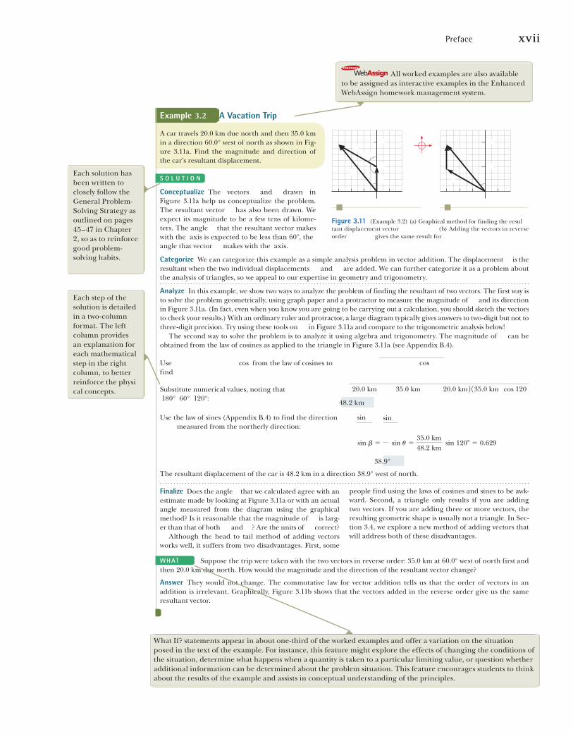
A car travels 20.0 km due north and then 35.0 km in a direction 60.0° west of north as shown in Fig-ure 3.11a. Find the magnitude and direction of the car’s resultant displacement.
Conceptualize The vectors and drawn in Figure 3.11a help us conceptualize the problem. The resultant vector has also been drawn. We expect its magnitude to be a few tens of kilome-ters. The angle that the resultant vector makes with the axis is expected to be less than 60°, the angle that vector makes with the axis.
Categorize We can categorize this example as a simple analysis problem in vector addition. The displacement is the resultant when the two individual displacements and are added. We can further categorize it as a problem about the analysis of triangles, so we appeal to our expertise in geometry and trigonometry.
Analyze In this example, we show two ways to analyze the problem of finding the resultant of two vectors. The first way is to solve the problem geometrically, using graph paper and a protractor to measure the magnitude of and its direction in Figure 3.11a. (In fact, even when you know you are going to be carrying out a calculation, you should sketch the vectors to check your results.) With an ordinary ruler and protractor, a large diagram typically gives answers to two-digit but not to three-digit precision. Try using these tools on in Figure 3.11a and compare to the trigonometric analysis below! The second way to solve the problem is to analyze it using algebra and trigonometry. The magnitude of can be obtained from the law of cosines as applied to the triangle in Figure 3.11a (see Appendix B.4).
S o l u t i o n
Use cos from the law of cosines to find
cos
Figure 3.11 (Example 3.2) (a) Graphical method for finding the resultant displacement vector (b) Adding the vectors in reverse order gives the same result for
Substitute numerical values, noting that 180° 60° 120°:
20.0 km 35.0 km 20.0 km 2 135.0 km cos 120
48.2 km
Use the law of sines (Appendix B.4) to find the direction measured from the northerly direction:
sin sin
sin b 5 sin u 535.0 km48.2 km
sin 1208 5 0.629
38.9°
The resultant displacement of the car is 48.2 km in a direction 38.9° west of north.
Finalize Does the angle that we calculated agree with an estimate made by looking at Figure 3.11a or with an actual angle measured from the diagram using the graphical method? Is it reasonable that the magnitude of is larg-er than that of both and ? Are the units of correct? Although the head to tail method of adding vectors works well, it suffers from two disadvantages. First, some
people find using the laws of cosines and sines to be awk-ward. Second, a triangle only results if you are adding two vectors. If you are adding three or more vectors, the resulting geometric shape is usually not a triangle. In Sec-tion 3.4, we explore a new method of adding vectors that will address both of these disadvantages.
Suppose the trip were taken with the two vectors in reverse order: 35.0 km at 60.0° west of north first and then 20.0 km due north. How would the magnitude and the direction of the resultant vector change?
Answer They would not change. The commutative law for vector addition tells us that the order of vectors in an addition is irrelevant. Graphically, Figure 3.11b shows that the vectors added in the reverse order give us the same resultant vector.
What
What If? statements appear in about one-third of the worked examples and offer a variation on the situation posed in the text of the example. For instance, this feature might explore the effects of changing the conditions of the situation, determine what happens when a quantity is taken to a particular limiting value, or question whether additional information can be determined about the problem situation. This feature encourages students to think about the results of the example and assists in conceptual understanding of the principles.
Each solution has been written to closely follow the General Problem-Solving Strategy as outlined on pages 45–47 in Chapter 2, so as to reinforce good problem-solving habits.
Each step of the solution is detailed in a two-column format. The left column provides an explanation for each mathematical step in the right column, to better reinforce the physical concepts.
All worked examples are also available to be assigned as interactive examples in the Enhanced WebAssign homework management system.
xviii Preface
Questions and Problems Sets. For the Ninth Edition, the authors reviewed each question and problem and incorporated revisions designed to improve both readability and assignability. More than 10% of the problems are new to this edition.
Questions. The Questions section is divided into two sections: Objective Questionsand Conceptual Questions. The instructor may select items to assign as homework or use in the classroom, possibly with “peer instruction” methods and possibly with personal response systems. More than 900 Objective and Conceptual Questions are included in this edition. Answers for selected questions are included in the Student Solutions Manual/Study Guide, and answers for all questions are found in the Instructor’s Solutions Manual.
Objective Questions are multiple-choice, true–false, ranking, or other multiple guess–type questions. Some require calculations designed to facilitate students’ familiarity with the equations, the variables used, the concepts the variables represent, and the relationships between the concepts. Others are more conceptual in nature and are designed to encourage conceptual thinking. Objective Questions are also written with the personal response system user in mind, and most of the questions could easily be used in these systems.
Conceptual Questions are more traditional short-answer and essay-type questions that require students to think conceptually about a physical situation.
Problems. An extensive set of problems is included at the end of each chapter; in all, this edition contains more than 3 700 problems. Answers for odd-numbered problems are provided at the end of the book. Full solutions for approximately 20% of the problems are included in the Student Solutions Manual/Study Guide, and solutions for all problems are found in the Instructor’s Solutions Manual.
The end-of-chapter problems are organized by the sections in each chapter (about two-thirds of the problems are keyed to specific sections of the chapter). Within each section, the problems now “platform” students to higher-order thinking by presenting all the straightforward problems in the section first, followed by the intermediate problems. (The problem numbers for straightforward problems are printed in black; intermediate-level problems are in blue.) The Additional Problems section contains problems that are not keyed to specific sections. At the end of each chapter is the Challenge Problems section, which gathers the most difficult problems for a given chapter in one place. (Challenge Problems have problem numbers marked in red.
There are several kinds of problems featured in this text:
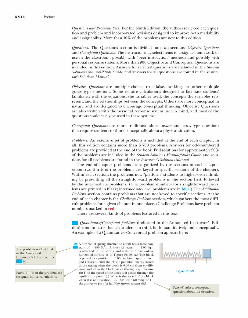
Quantitative/Conceptual problems (indicated in the Annotated Instructor’s Edition) contain parts that ask students to think both quantitatively and conceptually. An example of a Quantitative/Conceptual problem appears here:
242 Chapter Conservation of Energy
load a distance /2 in time interval /2, then (4) /2 will move /2 the given distance in the given time interval
(a) Show that Aristotle’s proportions are included in the equation bwd, where is a proportionality constant. (b) Show that our theory of motion includes this part of Aristotle’s theory as one special case. In particular, describe a situation in which it is true, derive the equation representing Aristotle’s proportions, and determine the proportionality constant.
61. A child’s pogo stick (Fig. P8.61) stores energy in a spring with a force constant of 2.50
N/m. At position 0.100 m), the spring com
pression is a maximum and the child is momentarily at rest. At position 0), the spring is relaxed and the child is moving upward. At position , the child is again momentarily at rest at the top of the jump. The combined mass of child and pogo stick is 25.0 kg. Although the boy must lean forward to remain balanced, the angle is small, so let’s assume the pogo stick is vertical. Also assume the boy does not bend his legs during the motion. (a) Calculate the total energy of the child–stick–Earth system, taking both gravitational and elastic potential energies as zero for
0. (b) Determine . (c) Calculate the speed of the child at 0. (d) Determine the value of for which the kinetic energy of the system is a maximum. (e) Calculate the child’s maximum upward speed.
62. A 1.00-kg object slides to the right on a surface having a coefficient of kinetic friction 0.250 (Fig. P8.62a). The object has a speed of 3.00 m/s when it makes contact with a light spring (Fig. P8.62b) that has a force constant of 50.0 N/m. The object comes to rest after the spring has been compressed a distance (Fig. P8.62c). The object is then forced toward the left by the spring (Fig. P8.62d) and continues to move in that direction beyond the spring’s unstretched position. Finally, the object comes to rest a distance to the left of the unstretched spring (Fig. P8.62e). Find (a) the distance of compression , (b) the speed at the unstretched position when the object is moving to the left (Fig. P8.62d), and (c) the distance where the object comes to rest.
Figure P8.61
Figure P8.62
(a) After the spring is compressed and the popgun fired, to what height does the projectile rise above point ? (b) Draw four energy bar charts for this situation, analogous to those in Figures 8.6c–d.
57. As the driver steps on the gas pedal, a car of mass 1 160 kg accelerates from rest. During the first few sec-onds of motion, the car’s acceleration increases with time according to the expression
1.16 0.210 0.240
where is in seconds and is in m/s . (a) What is the change in kinetic energy of the car during the interval from 0 to 2.50 s? (b) What is the minimum average power output of the engine over this time interval? (c) Why is the value in part (b) described as the minimum value?
58. Review. Why is the following situation impossible? A new high-speed roller coaster is claimed to be so safe that the passengers do not need to wear seat belts or any other restraining device. The coaster is designed with a vertical circular section over which the coaster trav-els on the inside of the circle so that the passengers are upside down for a short time interval. The radius of the circular section is 12.0 m, and the coaster enters the bottom of the circular section at a speed of 22.0 m/s. Assume the coaster moves without friction on the track and model the coaster as a particle.
59. A horizontal spring attached to a wall has a force con-stant of 850 N/m. A block of mass 1.00 kg is attached to the spring and rests on a frictionless, horizontal surface as in Figure P8.59. (a) The block is pulled to a position 6.00 cm from equilibrium and released. Find the elastic potential energy stored in the spring when the block is 6.00 cm from equilib-rium and when the block passes through equilibrium. (b) Find the speed of the block as it passes through the equilibrium point. (c) What is the speed of the block when it is at a position /2 3.00 cm? (d) Why isn’t the answer to part (c) half the answer to part (b)?
Figure P8.59
60. More than 2 300 years ago, the Greek teacher Aristo-tle wrote the first book called Physics. Put into more precise terminology, this passage is from the end of its Section Eta:
Let be the power of an agent causing motion; the load moved; , the distance covered; and , the time interval required. Then (1) a power
equal to will in an interval of time equal to move /2 a distance 2 or (2) it will move /2 the given distance in the time interval /2. Also, if (3) the given power moves the given
The problem is identified in the Annotated Instructor’s Edition with a
icon.
Parts (a)–(c) of the problem ask for quantitative calculations.
Part (d) asks a conceptual question about the situation.
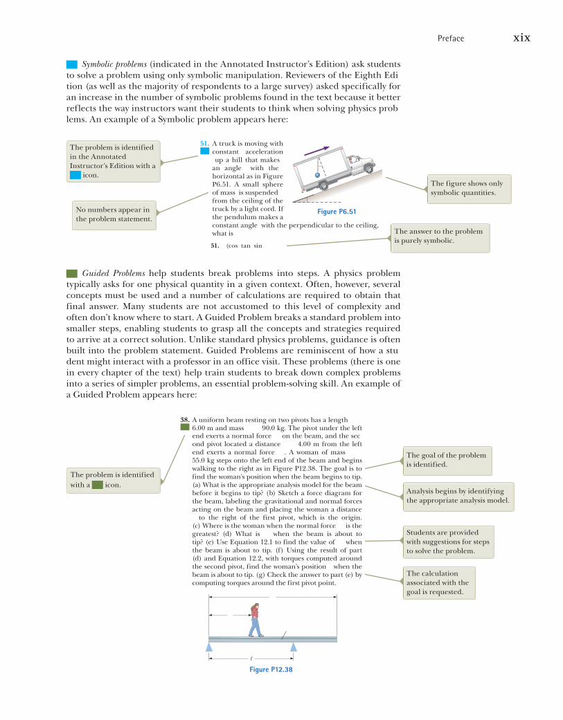
Preface xix
Symbolic problems (indicated in the Annotated Instructor’s Edition) ask students to solve a problem using only symbolic manipulation. Reviewers of the Eighth Edition (as well as the majority of respondents to a large survey) asked specifically for an increase in the number of symbolic problems found in the text because it better reflects the way instructors want their students to think when solving physics problems. An example of a Symbolic problem appears here:
174 Chapter Circular Motion and Other Applications of Newton’s Laws
in part (d) depend on the numerical values given in this problem, or is it true in general? Explain.
54. A puck of mass is tied to a string and allowed to revolve in a circle of radius on a frictionless, horizontal table. The other end of the string passes through a small hole in the center of the table, and an object of mass is tied to it (Fig. P6.54). The suspended object remains in equilibrium while the puck on the tabletop revolves. Find symbolic expressions for (a) the tension in the string, (b) the radial force acting on the puck, and (c) the speed of the puck. (d) Qualitatively describe what will happen in the motion of the puck if the value of is increased by placing a small additional load on the puck. (e) Qualitatively describe what will happen in the motion of the puck if the value of is instead decreased by removing a part of the hanging load.
55. Because the Earth rotates about its axis, a point on the equator experiences a centripetal acceleration of 0.0337 m/s , whereas a point at the poles experiences no centripetal acceleration. If a person at the equator has a mass of 75.0 kg, calculate (a) the gravitational force (true weight) on the person and (b) the normal force (apparent weight) on the person. (c) Which force is greater? Assume the Earth is a uniform sphere and take 9.800 m/s
Galileo thought about whether acceleration should be defined as the rate of change of velocity over time or as the rate of change in velocity over distance. He chose the former, so let’s use the name “vroomosity” for the rate of change of velocity over distance. For motion of a particle on a straight line with constant acceleration, the equation gives its velocity as a function of time. Similarly, for a particle’s linear motion with constant vroomosity , the equation gives the velocity as a function of the position if the particle’s speed is at 0. (a) Find the law describing the total force acting on this object of mass . (b) Describe an example of such a motion or explain why it is unrealistic. Consider (c) the possibility of positive and (d) the possibility of negative.
57. Figure P6.57 shows a photo of a swing ride at an amusement park. The structure consists of a horizontal, rotating, circular platform of diameter
from which seats of mass are suspended at the end of massless chains of length . When the system rotates at
Figure P6.54
Figure P6.57
Stua
rt G
rego
ry/G
etty
Imag
es
AMT
separation from the line of best fit. Express this scatter as a percentage. (e) In a short paragraph, state what the graph demonstrates and compare it with the the-oretical prediction. You will need to make reference to the quantities plotted on the axes, to the shape of the graph line, to the data points, and to the results of parts (c) and (d).
50. A basin surrounding a drain has the shape of a circular cone opening upward, having everywhere an angle of 35.0° with the horizontal. A 25.0-g ice cube is set sliding around the cone without friction in a horizontal circle of radius . (a) Find the speed the ice cube must have as a function of . (b) Is any piece of data unnecessary for the solution? Suppose is made two times larger. (c) Will the required speed increase, decrease, or stay constant? If it changes, by what factor? (d) Will the time required for each revolution increase, decrease, or stay constant? If it changes, by what factor? (e) Do the answers to parts (c) and (d) seem contradictory? Explain.
51. A truck is moving with constant acceleration up a hill that makes an angle with the horizontal as in Figure P6.51. A small sphere of mass is suspended from the ceiling of the truck by a light cord. If the pendulum makes a constant angle with the perpendicular to the ceiling, what is
52. The pilot of an airplane executes a loop-the-loop maneuver in a vertical circle. The speed of the airplane is 300 mi/h at the top of the loop and 450 mi/h at the bottom, and the radius of the circle is 1 200 ft. (a) What is the pilot’s apparent weight at the lowest point if his true weight is 160 lb? (b) What is his apparent weight at the highest point? (c) What If? Describe how the pilot could experience weightlessness if both the radius and the speed can be varied. Note: His apparent weight is equal to the magnitude of the force exerted by the seat on his body.
53. Review. While learning to drive, you are in a 1 200-kg car moving at 20.0 m/s across a large, vacant, level parking lot. Suddenly you realize you are heading straight toward the brick sidewall of a large supermar-ket and are in danger of running into it. The pavement can exert a maximum horizontal force of 7 000 N on the car. (a) Explain why you should expect the force to have a well-defined maximum value. (b) Suppose you apply the brakes and do not turn the steering wheel. Find the minimum distance you must be from the wall to avoid a collision. (c) If you do not brake but instead maintain constant speed and turn the steering wheel, what is the minimum distance you must be from the wall to avoid a collision? (d) Of the two methods in parts (b) and (c), which is better for avoiding a colli-sion? Or should you use both the brakes and the steer-ing wheel, or neither? Explain. (e) Does the conclusion
Figure P6.51No numbers appear in the problem statement.
The answer to the problem is purely symbolic.
51. (cos tan sin
The figure shows only symbolic quantities.
The problem is identified in the Annotated Instructor’s Edition with a
icon.
Guided Problems help students break problems into steps. A physics problem typically asks for one physical quantity in a given context. Often, however, several concepts must be used and a number of calculations are required to obtain that final answer. Many students are not accustomed to this level of complexity and often don’t know where to start. A Guided Problem breaks a standard problem into smaller steps, enabling students to grasp all the concepts and strategies required to arrive at a correct solution. Unlike standard physics problems, guidance is often built into the problem statement. Guided Problems are reminiscent of how a student might interact with a professor in an office visit. These problems (there is one in every chapter of the text) help train students to break down complex problems into a series of simpler problems, an essential problem-solving skill. An example of a Guided Problem appears here:
Problems 383
end exerts a normal force on the beam, and the second pivot located a distance 4.00 m from the left end exerts a normal force . A woman of mass 55.0 kg steps onto the left end of the beam and begins walking to the right as in Figure P12.38. The goal is to find the woman’s position when the beam begins to tip. (a) What is the appropriate analysis model for the beam before it begins to tip? (b) Sketch a force diagram for the beam, labeling the gravitational and normal forces acting on the beam and placing the woman a distance to the right of the first pivot, which is the origin.
(c) Where is the woman when the normal force is the greatest? (d) What is when the beam is about to tip? (e) Use Equation 12.1 to find the value of when the beam is about to tip. (f) Using the result of part (d) and Equation 12.2, with torques computed around the second pivot, find the woman’s position when the beam is about to tip. (g) Check the answer to part (e) by computing torques around the first pivot point.
Figure P12.38
39. In exercise physiology studies, it is sometimes important to determine the location of a person’s center of mass. This determination can be done with the arrangement shown in Figure P12.39. A light plank rests on two scales, which read 380 N and 320 N. A distance of 1.65 m separates the scales. How far from the woman’s feet is her center of mass?
Figure P12.39
40. The lintel of prestressed reinforced concrete in Fig-ure P12.40 is 1.50 m long. The concrete encloses one steel reinforcing rod with cross-sectional area 1.50 cm . The rod joins two strong end plates. The cross- sectional area of the concrete perpendicular to the rod is 50.0 cm . Young’s modulus for the concrete is 30.0 10 N/m . After the concrete cures and the original tension in the rod is released, the concrete is to be under compres-sive stress 8.00 10 N/m . (a) By what distance will the rod compress the concrete when the original tension in the rod is released? (b) What
30. Evaluate Young’s modulus for the material whose stress–strain curve is shown in Figure 12.12.
31. Assume if the shear stress in steel exceeds about 4.00 N/m , the steel ruptures. Determine the shear-
ing force necessary to (a) shear a steel bolt 1.00 cm in diameter and (b) punch a 1.00-cm-diameter hole in a steel plate 0.500 cm thick.
32. When water freezes, it expands by about 9.00%. What pressure increase would occur inside your automobile engine block if the water in it froze? (The bulk modu-lus of ice is 2.00 10 N/m
33. A 200-kg load is hung on a wire of length 4.00 m, cross-sectional area 0.200 10 , and Young’s modulus 8.00 10 N/m . What is its increase in length?
34. A walkway suspended across a hotel lobby is supported at numerous points along its edges by a vertical cable above each point and a vertical column underneath. The steel cable is 1.27 cm in diameter and is 5.75 m long before loading. The aluminum column is a hollow cylinder with an inside diameter of 16.14 cm, an outside diameter of 16.24 cm, and an unloaded length of 3.25 m. When the walkway exerts a load force of 8 500 N on one of the support points, how much does the point move down?
35. Review. A 2.00-m-long cylindrical steel wire with a cross-sectional diameter of 4.00 mm is placed over a light, frictionless pulley. An object of mass
5.00 kg is hung from one end of the wire and an object of mass 3.00 kg from the other end as shown in Figure P12.35. The objects are released and allowed to move freely. Compared with its length before the objects were attached, by how much has the wire stretched while the objects are in motion?
36. Review. A 30.0-kg hammer, moving with speed 20.0 m/s, strikes a steel spike 2.30 cm in diameter. The hammer rebounds with speed 10.0 m/s after 0.110 s. What is the average strain in the spike during the impact?
Additional Problems
37. A bridge of length 50.0 m and mass 8.00 10 kg is supported on a smooth pier at each end as shown in Figure P12.37. A truck of mass 3.00 10 kg is located 15.0 m from one end. What are the forces on the bridge at the points of support?
Figure P12.37
38. A uniform beam resting on two pivots has a length 6.00 m and mass 90.0 kg. The pivot under the left
AMT
Figure P12.35
Figure P12.40
The goal of the problem is identified.
Analysis begins by identifying the appropriate analysis model.
Students are provided with suggestions for steps to solve the problem.
The problem is identified with a icon.
The calculation associated with the goal is requested.
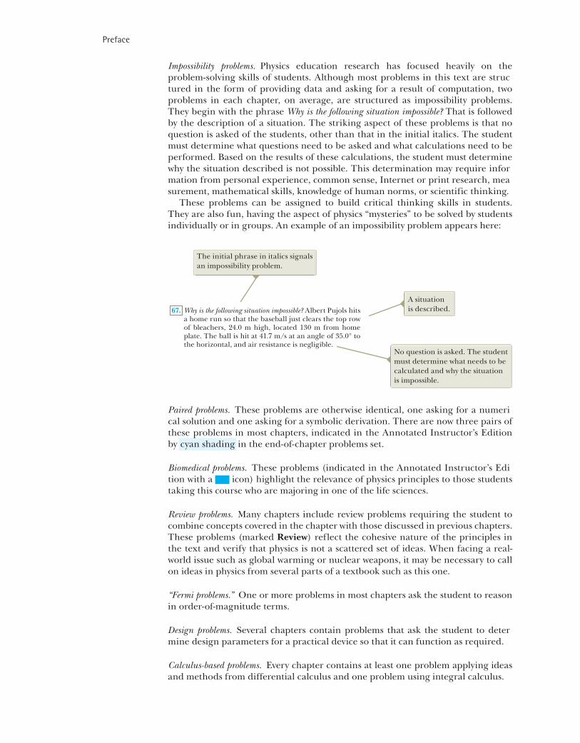
Preface
Impossibility problems. Physics education research has focused heavily on the problem-solving skills of students. Although most problems in this text are structured in the form of providing data and asking for a result of computation, two problems in each chapter, on average, are structured as impossibility problems. They begin with the phrase Why is the following situation impossible? That is followed by the description of a situation. The striking aspect of these problems is that no question is asked of the students, other than that in the initial italics. The student must determine what questions need to be asked and what calculations need to be performed. Based on the results of these calculations, the student must determine why the situation described is not possible. This determination may require information from personal experience, common sense, Internet or print research, measurement, mathematical skills, knowledge of human norms, or scientific thinking.
These problems can be assigned to build critical thinking skills in students. They are also fun, having the aspect of physics “mysteries” to be solved by students individually or in groups. An example of an impossibility problem appears here:
Paired problems. These problems are otherwise identical, one asking for a numerical solution and one asking for a symbolic derivation. There are now three pairs of these problems in most chapters, indicated in the Annotated Instructor’s Edition by cyan shading in the end-of-chapter problems set.
Biomedical problems. These problems (indicated in the Annotated Instructor’s Edition with a icon) highlight the relevance of physics principles to those students taking this course who are majoring in one of the life sciences.
Review problems. Many chapters include review problems requiring the student to combine concepts covered in the chapter with those discussed in previous chapters. These problems (marked Review) reflect the cohesive nature of the principles in the text and verify that physics is not a scattered set of ideas. When facing a real-world issue such as global warming or nuclear weapons, it may be necessary to call on ideas in physics from several parts of a textbook such as this one.
“Fermi problems.” One or more problems in most chapters ask the student to reason in order-of-magnitude terms.
Design problems. Several chapters contain problems that ask the student to determine design parameters for a practical device so that it can function as required.
Calculus-based problems. Every chapter contains at least one problem applying ideas and methods from differential calculus and one problem using integral calculus.
The initial phrase in italics signals an impossibility problem.
A situation is described.
Problems 107
leave simultaneously and drive for 2.50 h in the direc-tions shown. Car 1 has a speed of 90.0 km/h. If the cars arrive simultaneously at the lake, what is the speed of car 2?
Figure P4.64
65. A catapult launches a rocket at an angle of 53.0° above the horizontal with an initial speed of 100 m/s. The rocket engine immediately starts a burn, and for 3.00 s the rocket moves along its initial line of motion with an acceleration of 30.0 m/s . Then its engine fails, and the rocket proceeds to move in free fall. Find (a) the maximum altitude reached by the rocket, (b) its total time of flight, and (c) its horizontal range.
66. A cannon with a muzzle speed of 1 000 m/s is used to start an avalanche on a mountain slope. The target is 2 000 m from the cannon horizontally and 800 m above the cannon. At what angle, above the horizontal, should the cannon be fired?
67. Why is the following situation impossible? Albert Pujols hits a home run so that the baseball just clears the top row of bleachers, 24.0 m high, located 130 m from home plate. The ball is hit at 41.7 m/s at an angle of 35.0° to the horizontal, and air resistance is negligible.
68. As some molten metal splashes, one droplet flies off to the east with initial velocity at angle above the horizontal, and another droplet flies off to the west with the same speed at the same angle above the horizontal as shown in Figure P4.68. In terms of and , find the distance between the two droplets as a function of time.
Figure P4.68
69. An astronaut on the surface of the Moon fires a can-non to launch an experiment package, which leaves the barrel moving horizontally. Assume the free-fall acceleration on the Moon is one-sixth of that on the
it enters a parabolic path with a velocity of 143 m/s nose high at 45.0° and exits with velocity 143 m/s at 45.0° nose low. During this portion of the flight, the aircraft and objects inside its padded cabin are in free fall; astronauts and equipment float freely as if there were no gravity. What are the aircraft’s (a) speed and (b) altitude at the top of the maneuver? (c) What is the time interval spent in microgravity?
60. A basketball player is standing on the floor 10.0 m from the basket as in Figure P4.60. The height of the basket is 3.05 m, and he shoots the ball at a 40.0 angle with the horizontal from a height of 2.00 m. (a) What is the acceleration of the basketball at the highest point in its trajectory? (b) At what speed must the player throw the basketball so that the ball goes through the hoop without striking the backboard?
Figure P4.60
61. Lisa in her Lamborghini accelerates at the rate of 3.00 2.00 m/s , while Jill in her Jaguar acceler
ates at 1.00 3.00 m/s . They both start from rest at the origin of an coordinate system. After 5.00 s, (a) what is Lisa’s speed with respect to Jill, (b) how far apart are they, and (c) what is Lisa’s acceleration relative to Jill?
62. A boy throws a stone horizontally from the top of a cliff of height toward the ocean below. The stone strikes the ocean at distance from the base of the cliff. In terms of h, d, and , find expressions for (a) the time at which the stone lands in the ocean, (b) the initial speed of the stone, (c) the speed of the stone immedi-ately before it reaches the ocean, and (d) the direction of the stone’s velocity immediately before it reaches the ocean.
63. A flea is at point on a horizontal turntable, 10.0 cm from the center. The turntable is rotating at 33.3 rev/min in the clockwise direction. The flea jumps straight up to a height of 5.00 cm. At takeoff, it gives itself no hori-zontal velocity relative to the turntable. The flea lands on the turntable at point . Choose the origin of coordinates to be at the center of the turntable and the positive axis passing through at the moment of takeoff. Then the original position of the flea is 10.0 cm. (a) Find the position of point when the flea lands. (b) Find the position of point when the flea lands.
64. Towns A and B in Figure P4.64 are 80.0 km apart. A couple arranges to drive from town A and meet a cou-ple driving from town B at the lake, L. The two couples
No question is asked. The student must determine what needs to be calculated and why the situation is impossible.
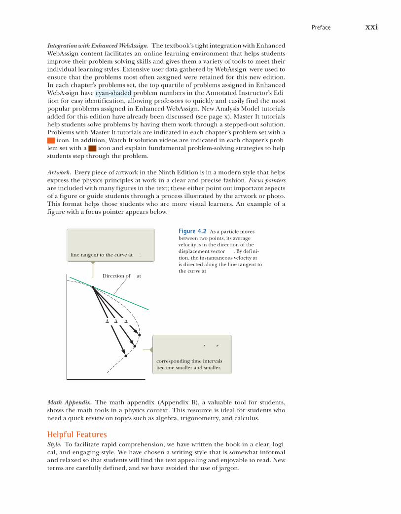
Preface xxi
Integration with Enhanced WebAssign. The textbook’s tight integration with Enhanced WebAssign content facilitates an online learning environment that helps students improve their problem-solving skills and gives them a variety of tools to meet their individual learning styles. Extensive user data gathered by WebAssign were used to ensure that the problems most often assigned were retained for this new edition. In each chapter’s problems set, the top quartile of problems assigned in Enhanced WebAssign have cyan-shaded problem numbers in the Annotated Instructor’s Edition for easy identification, allowing professors to quickly and easily find the most popular problems assigned in Enhanced WebAssign. New Analysis Model tutorials added for this edition have already been discussed (see page x). Master It tutorials help students solve problems by having them work through a stepped-out solution. Problems with Master It tutorials are indicated in each chapter’s problem set with a
icon. In addition, Watch It solution videos are indicated in each chapter’s problem set with a icon and explain fundamental problem-solving strategies to help students step through the problem.
Artwork. Every piece of artwork in the Ninth Edition is in a modern style that helps express the physics principles at work in a clear and precise fashion. Focus pointersare included with many figures in the text; these either point out important aspects of a figure or guide students through a process illustrated by the artwork or photo. This format helps those students who are more visual learners. An example of a figure with a focus pointer appears below.
���
Direction of at
line tangent to the curve at .
corresponding time intervals become smaller and smaller.
� �
Figure 4.2 As a particle moves between two points, its average velocity is in the direction of the displacement vector . By defini-tion, the instantaneous velocity at is directed along the line tangent to the curve at
Math Appendix. The math appendix (Appendix B), a valuable tool for students, shows the math tools in a physics context. This resource is ideal for students who need a quick review on topics such as algebra, trigonometry, and calculus.
Helpful FeaturesStyle. To facilitate rapid comprehension, we have written the book in a clear, logical, and engaging style. We have chosen a writing style that is somewhat informal and relaxed so that students will find the text appealing and enjoyable to read. New terms are carefully defined, and we have avoided the use of jargon.

xxii Preface
Important Definitions and Equations. Most important definitions are set in bold-face or are highlighted with a background screen for added emphasis and ease of review. Similarly, important equations are also highlighted with a background screen to facilitate location.
Marginal Notes. Comments and notes appearing in the margin with a icon can be used to locate important statements, equations, and concepts in the text.
Pedagogical Use of Color. Readers should consult the pedagogical color chart (inside the front cover) for a listing of the color-coded symbols used in the text diagrams. This system is followed consistently throughout the text.
Mathematical Level. We have introduced calculus gradually, keeping in mind that students often take introductory courses in calculus and physics concurrently. Most steps are shown when basic equations are developed, and reference is often made to mathematical appendices near the end of the textbook. Although vectors are discussed in detail in Chapter 3, vector products are introduced later in the text, where they are needed in physical applications. The dot product is introduced in Chapter 7, which addresses energy of a system; the cross product is introduced in Chapter 11, which deals with angular momentum.
Significant Figures. In both worked examples and end-of-chapter problems, signifi-cant figures have been handled with care. Most numerical examples are worked to either two or three significant figures, depending on the precision of the data provided. End-of-chapter problems regularly state data and answers to three-digit precision. When carrying out estimation calculations, we shall typically work with a single significant figure. (More discussion of significant figures can be found in Chapter 1, pages 11–13.)
Units. The international system of units (SI) is used throughout the text. The U.S. customary system of units is used only to a limited extent in the chapters on mechanics and thermodynamics.
Appendices and Endpapers. Several appendices are provided near the end of the textbook. Most of the appendix material represents a review of mathematical con-cepts and techniques used in the text, including scientific notation, algebra, geom-etry, trigonometry, differential calculus, and integral calculus. Reference to these appendices is made throughout the text. Most mathematical review sections in the appendices include worked examples and exercises with answers. In addition to the mathematical reviews, the appendices contain tables of physical data, conversion factors, and the SI units of physical quantities as well as a periodic table of the ele-ments. Other useful information—fundamental constants and physical data, plan-etary data, a list of standard prefixes, mathematical symbols, the Greek alphabet, and standard abbreviations of units of measure—appears on the endpapers.
CengageCompose Options for Physics for Scientists and Engineers
Would you like to easily create your own personalized text, selecting the elements that meet your specific learning objectives? CengageCompose puts the power of the vast Cengage Learning library of learn-ing content at your fingertips to create exactly the text you need. The all-new, Web-based CengageCompose site lets you quickly scan content and review materials to pick what you need for your text. Site tools let you easily assemble the modular learn-ing units into the order you want and immediately provide you with an online copy for review. Add enrichment content like case studies, exercises, and lab materials to

Preface xxiii
further build your ideal learning materials. Even choose from hundreds of vivid, art-rich, customizable, full-color covers.
Cengage Learning offers the fastest and easiest way to create unique customized learning materials delivered the way you want. For more information about custom publishing options, visit www.cengage.com/custom or contact your local Cengage Learning representative.
Course Solutions That Fit Your Teaching Goals and Your Students’ Learning Needs
Recent advances in educational technology have made homework management systems and audience response systems powerful and affordable tools to enhance the way you teach your course. Whether you offer a more traditional text-based course, are interested in using or are currently using an online homework management system such as Enhanced WebAssign, or are ready to turn your lecture into an interactive learning environment with JoinIn, you can be confident that the text’s proven content provides the foundation for each and every component of our technology and ancillary package.
Homework Management SystemsEnhanced WebAssign for Physics for Scientists and Engineers, Ninth Edition. Exclusively from Cengage Learning, Enhanced WebAssign offers an extensive online program for physics to encourage the practice that’s so critical for concept mastery. The meticulously crafted pedagogy and exercises in our proven texts become even more effective in Enhanced WebAssign. Enhanced WebAssign includes the Cengage YouBook, a highly customizable, interactive eBook. WebAssign includes:
All of the quantitative end-of-chapter problemsSelected problems enhanced with targeted feedback. An example of tar-geted feedback appears below:
Selected problems include feedback to address common mistakes that students make. This feedback was developed by professors with years of classroom experience.
Master It tutorials (indicated in the text by a icon), to help students work through the problem one step at a time. An example of a Master It tutorial appears on page xxiv:
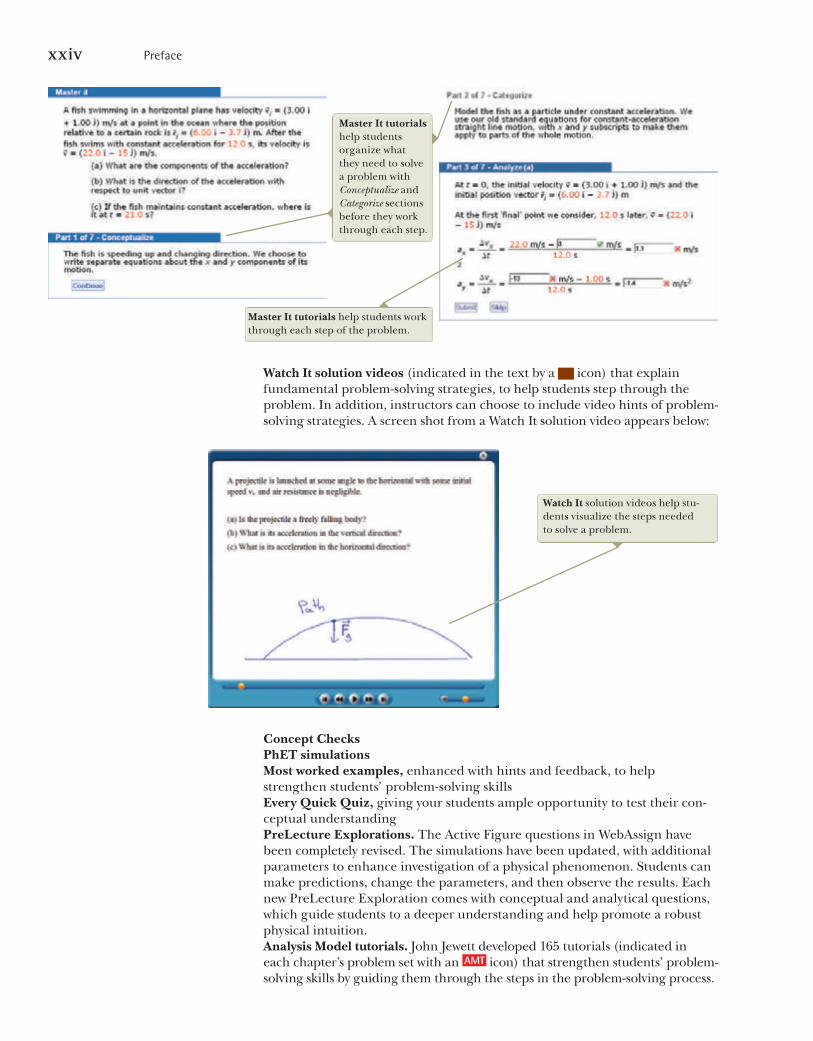
xxiv Preface
Watch It solution videos (indicated in the text by a icon) that explain fundamental problem-solving strategies, to help students step through the problem. In addition, instructors can choose to include video hints of problem-solving strategies. A screen shot from a Watch It solution video appears below:
Master It tutorialshelp students organize what they need to solve a problem with Conceptualize and Categorize sections before they work through each step.
Master It tutorials help students work through each step of the problem.
Watch It solution videos help stu-dents visualize the steps needed to solve a problem.
Concept ChecksPhET simulationsMost worked examples, enhanced with hints and feedback, to help strengthen students’ problem-solving skillsEvery Quick Quiz, giving your students ample opportunity to test their con-ceptual understandingPreLecture Explorations. The Active Figure questions in WebAssign have been completely revised. The simulations have been updated, with additional parameters to enhance investigation of a physical phenomenon. Students can make predictions, change the parameters, and then observe the results. Each new PreLecture Exploration comes with conceptual and analytical questions, which guide students to a deeper understanding and help promote a robust physical intuition.Analysis Model tutorials. John Jewett developed 165 tutorials (indicated in each chapter’s problem set with an AMT icon) that strengthen students’ problem-solving skills by guiding them through the steps in the problem-solving process.
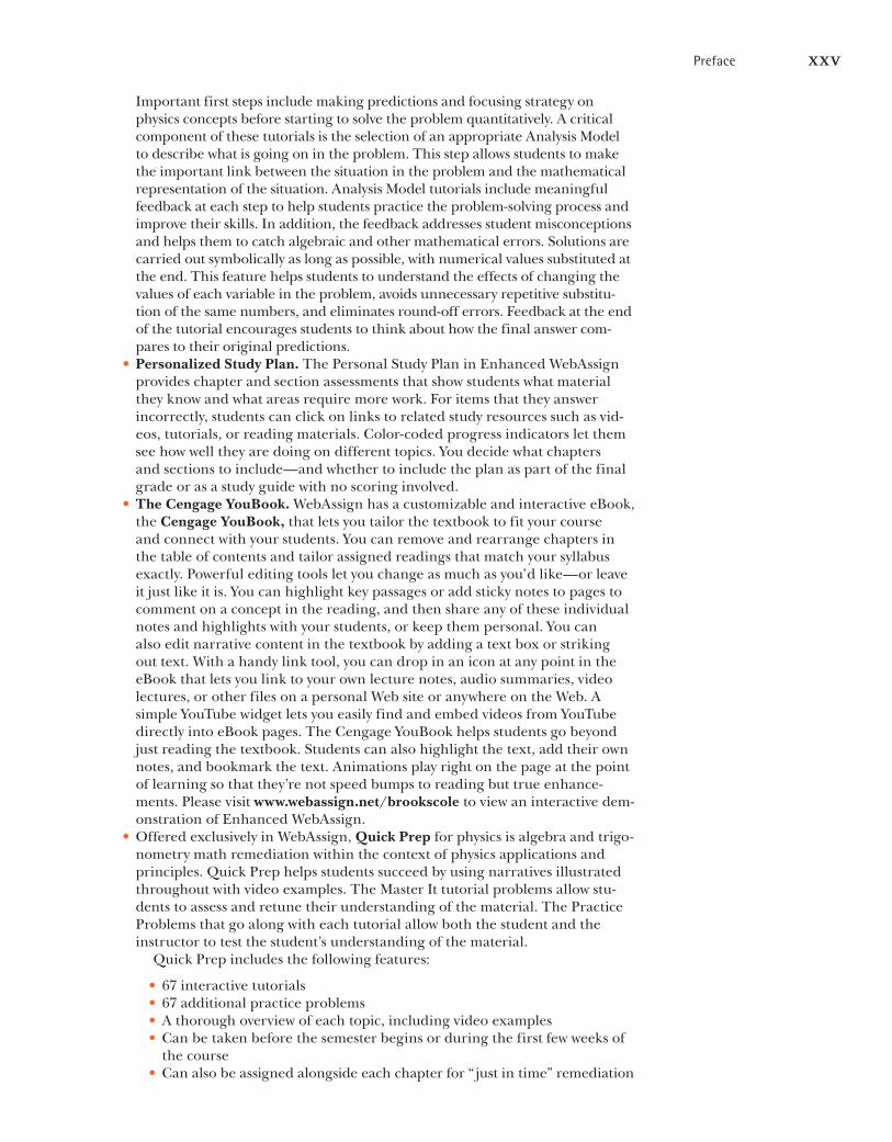
Preface xxv
Important first steps include making predictions and focusing strategy on physics concepts before starting to solve the problem quantitatively. A critical component of these tutorials is the selection of an appropriate Analysis Model to describe what is going on in the problem. This step allows students to make the important link between the situation in the problem and the mathematical representation of the situation. Analysis Model tutorials include meaningful feedback at each step to help students practice the problem-solving process and improve their skills. In addition, the feedback addresses student misconceptions and helps them to catch algebraic and other mathematical errors. Solutions are carried out symbolically as long as possible, with numerical values substituted at the end. This feature helps students to understand the effects of changing the values of each variable in the problem, avoids unnecessary repetitive substitu-tion of the same numbers, and eliminates round-off errors. Feedback at the end of the tutorial encourages students to think about how the final answer com-pares to their original predictions.
•Personalized Study Plan. The Personal Study Plan in Enhanced WebAssign provides chapter and section assessments that show students what material they know and what areas require more work. For items that they answer incorrectly, students can click on links to related study resources such as vid-eos, tutorials, or reading materials. Color-coded progress indicators let them see how well they are doing on different topics. You decide what chapters and sections to include—and whether to include the plan as part of the final grade or as a study guide with no scoring involved.
•The Cengage YouBook. WebAssign has a customizable and interactive eBook, the Cengage YouBook, that lets you tailor the textbook to fit your course and connect with your students. You can remove and rearrange chapters in the table of contents and tailor assigned readings that match your syllabus exactly. Powerful editing tools let you change as much as you’d like—or leave it just like it is. You can highlight key passages or add sticky notes to pages to comment on a concept in the reading, and then share any of these individual notes and highlights with your students, or keep them personal. You can also edit narrative content in the textbook by adding a text box or striking out text. With a handy link tool, you can drop in an icon at any point in the eBook that lets you link to your own lecture notes, audio summaries, video lectures, or other files on a personal Web site or anywhere on the Web. A simple YouTube widget lets you easily find and embed videos from YouTube directly into eBook pages. The Cengage YouBook helps students go beyond just reading the textbook. Students can also highlight the text, add their own notes, and bookmark the text. Animations play right on the page at the point of learning so that they’re not speed bumps to reading but true enhance-ments. Please visit www.webassign.net/brookscole to view an interactive dem-onstration of Enhanced WebAssign.
•Offered exclusively in WebAssign, Quick Prep for physics is algebra and trigo-nometry math remediation within the context of physics applications and principles. Quick Prep helps students succeed by using narratives illustrated throughout with video examples. The Master It tutorial problems allow stu-dents to assess and retune their understanding of the material. The Practice Problems that go along with each tutorial allow both the student and the instructor to test the student’s understanding of the material.
Quick Prep includes the following features:
• 67 interactive tutorials• 67 additional practice problems•A thorough overview of each topic, including video examples•Can be taken before the semester begins or during the first few weeks of
the course•Can also be assigned alongside each chapter for “ just in time” remediation

xxvi Preface
Topics include units, scientific notation, and significant figures; the motion of objects along a line; functions; approximation and graphing; probability and error; vectors, displacement, and velocity; spheres; force and vector projections.
MindTap™: The Personal Learning ExperienceMindTap for Serway and Jewett Physics for Scientists and Engineers is a personalized, fully online digital learning platform of authoritative textbook content, assignments, and services that engages your students with interactivity while also offering you choice in the configuration of coursework and enhancement of the curriculum via complimentary Web-apps known as MindApps. MindApps range from ReadSpeaker (which reads the text out loud to students), to Kaltura (allowing you to insert inline video and audio into your curriculum), to ConnectYard (allowing you to create digi-tal “yards” through social media—all without “friending” your students). MindTap is well beyond an eBook, a homework solution or digital supplement, a resource center Web site, a course delivery platform, or a Learning Management System. It is the first in a new category—the Personal Learning Experience.
CengageBrain.comOn CengageBrain.com students will be able to save up to 60% on their course mate-rials through our full spectrum of options. Students will have the option to rent their textbooks, purchase print textbooks, e-textbooks, or individual e-chapters and audio books all for substantial savings over average retail prices. CengageBrain.com also includes access to Cengage Learning’s broad range of homework and study tools and features a selection of free content.
Lecture Presentation ResourcesPowerLecture with ExamView® and JoinIn for Physics for Scientists and Engineers, Ninth Edition. Bringing physics principles and concepts to life in your lectures has never been easier! The full-featured, two-volume PowerLecture Instructor’s Resource DVD-ROM (Volume 1: Chapters 1–22; Volume 2: Chapters 23–46) pro-vides everything you need for Physics for Scientists and Engineers, Ninth Edition. Key content includes the Instructor’s Solutions Manual, art and images from the text, pre-made chapter-specific PowerPoint lectures, ExamView test generator software with pre-loaded test questions, JoinIn response-system “clickers,” Active Figures anima-tions, and a physics movie library.
JoinIn. Assessing to Learn in the Classroom questions developed at the University of Massachusetts Amherst. This collection of 250 advanced conceptual questions has been tested in the classroom for more than ten years and takes peer learning to a new level. JoinIn helps you turn your lectures into an interactive learning envi-ronment that promotes conceptual understanding. Available exclusively for higher education from our partnership with Turning Technologies, JoinIn™ is the easiest way to turn your lecture hall into a personal, fully interactive experience for your students!
Assessment and Course Preparation ResourcesA number of resources listed below will assist with your assessment and preparation processes.
Instructor’s Solutions Manual by Vahé Peroomian (University of California at Los Angeles). Thoroughly revised for this edition, the Instructor’s Solutions Manual contains complete worked solutions to all end-of-chapter problems in the textbook as well as answers to the even- numbered problems and all the questions. The solutions to prob-lems new to the Ninth Edition are marked for easy identification. Volume 1 contains Chapters 1 through 22; Volume 2 contains Chapters 23 through 46. Electronic files of the Instructor’s Solutions Manual are available on the PowerLecture™ DVD-ROM.

Preface xxvii
Test Bank by Ed Oberhofer (University of North Carolina at Charlotte and Lake Sumter Community College). The test bank is available on the two-volume PowerLecture™ DVD-ROM via the ExamView® test software. This two-volume test bank contains approximately 2 000 multiple-choice questions. Instructors may print and duplicate pages for distribution to students. Volume 1 contains Chapters 1 through 22, and Volume 2 contains Chapters 23 through 46. WebCT and Blackboard versions of the test bank are available on the instructor’s companion site at www.CengageBrain.com.
Instructor’s Companion Web Site. Consult the instructor’s site by pointing your browser to www.CengageBrain.com for a problem correlation guide, PowerPoint lectures, and JoinIn audience response content. Instructors adopting the Ninth Edition of Physics for Scientists and Engineers may download these materials after securing the appropriate password from their local sales representative.
Supporting Materials for the InstructorSupporting instructor materials are available to qualified adopters. Please con-sult your local Cengage Learning, Brooks/Cole representative for details. Visit www.CengageBrain.com to
• request a desk copy• locate your local representative• download electronic files of select support materials
Student ResourcesVisit the Physics for Scientists and Engineers Web site at www.cengagebrain.com/ shop/ISBN/9781133954156 to see samples of select student supplements. Go to CengageBrain.com to purchase and access this product at Cengage Learning’s pre-ferred online store.
Student Solutions Manual/Study Guide by John R. Gordon, Vahé Peroomian, Raymond A. Serway, and John W. Jewett, Jr. This two-volume manual features detailed solu-tions to 20% of the end-of-chapter problems from the text. The manual also fea-tures a list of important equations, concepts, and notes from key sections of the text in addition to answers to selected end-of-chapter questions. Volume 1 contains Chapters 1 through 22; and Volume 2 contains Chapters 23 through 46.
Physics Laboratory Manual, Third Edition by David Loyd (Angelo State University) supplements the learning of basic physical principles while introducing laboratory procedures and equipment. Each chapter includes a prelaboratory assignment, objectives, an equipment list, the theory behind the experiment, experimental pro-cedures, graphing exercises, and questions. A laboratory report form is included with each experiment so that the student can record data, calculations, and experi-mental results. Students are encouraged to apply statistical analysis to their data. A complete Instructor’s Manual is also available to facilitate use of this lab manual.
Physics Laboratory Experiments, Seventh Edition by Jerry D. Wilson (Lander College) and Cecilia A. Hernández (American River College). This market-leading manual for the first-year physics laboratory course offers a wide range of class-tested experiments designed specifically for use in small to midsize lab programs. A series of integrated experiments emphasizes the use of computerized instrumentation and includes a set of “computer-assisted experiments” to allow students and instructors to gain experience with modern equipment. This option also enables instructors to determine the appropriate balance between traditional and computer-based experiments for their courses. By analyzing data through two different methods, students gain a greater understanding of the concepts behind the experiments. The Seventh Edition is updated with the latest information and techniques involving state-of-the-art equipment and a new Guided Learning feature addresses

xxviii Preface
the growing interest in guided-inquiry pedagogy. Fourteen additional experiments are also available through custom printing.
Teaching OptionsThe topics in this textbook are presented in the following sequence: classical mechan-ics, oscillations and mechanical waves, and heat and thermodynamics, followed by electricity and magnetism, electromagnetic waves, optics, relativity, and modern phys-ics. This presentation represents a traditional sequence, with the subject of mechani-cal waves being presented before electricity and magnetism. Some instructors may prefer to discuss both mechanical and electromagnetic waves together after complet-ing electricity and magnetism. In this case, Chapters 16 through 18 could be covered along with Chapter 34. The chapter on relativity is placed near the end of the text because this topic often is treated as an introduction to the era of “modern physics.” If time permits, instructors may choose to cover Chapter 39 after completing Chapter 13 as a conclusion to the material on Newtonian mechanics. For those instructors teach-ing a two-semester sequence, some sections and chapters could be deleted without any loss of continuity. The following sections can be considered optional for this purpose:
2.8 Kinematic Equations Derived from Calculus 4.6 Relative Velocity and Relative Acceleration 6.3 Motion in Accelerated Frames 6.4 Motion in the Presence of Resistive Forces 7.9 Energy Diagrams and Equilibrium of a System 9.9 Rocket Propulsion 11.5 The Motion of Gyroscopes and Tops 14.7 Other Applications of Fluid Dynamics 15.6 Damped Oscillations 15.7 Forced Oscillations 18.6 Standing Waves in Rods and Membranes 18.8 Nonsinusoidal Wave Patterns 25.7 The Millikan Oil-Drop Experiment 25.8 Applications of Electrostatics 26.7 An Atomic Description of Dielectrics 27.5 Superconductors 28.5 Household Wiring and Electrical Safety 29.3 Applications Involving Charged Particles
Moving in a Magnetic Field 29.6 The Hall Effect 30.6 Magnetism in Matter
31.6 Eddy Currents 33.9 Rectifiers and Filters 34.6 Production of Electromagnetic Waves
by an Antenna 36.5 Lens Aberrations 36.6 The Camera 36.7 The Eye 36.8 The Simple Magnifier 36.9 The Compound Microscope 36.10 The Telescope 38.5 Diffraction of X-Rays by Crystals 39.9 The General Theory of Relativity 41.6 Applications of Tunneling 42.9 Spontaneous and Stimulated Transitions 42.10 Lasers 43.7 Semiconductor Devices 43.8 Superconductivity 44.8 Nuclear Magnetic Resonance and
Magnetic Resonance Imaging 45.5 Radiation Damage 45.6 Uses of Radiation
AcknowledgmentsThis Ninth Edition of Physics for Scientists and Engineers was prepared with the guid-ance and assistance of many professors who reviewed selections of the manuscript, the prerevision text, or both. We wish to acknowledge the following scholars and express our sincere appreciation for their suggestions, criticisms, and encouragement:
Benjamin C. Bromley, University of Utah; Elena Flitsiyan, University of Central Florida; Yuankun Lin, University of North Texas; Allen Mincer, New York University; Yibin Pan, University of Wisconsin–Madison; N. M. Ravindra, New Jersey Institute of Technology; Masao Sako, University of Pennsylvania; Charles Stone, Colorado School of Mines; Robert Weid-man, Michigan Technological University; Michael Winokur, University of Wisconsin–Madison
Prior to our work on this revision, we conducted a survey of professors; their feedback and suggestions helped shape this revision, and so we would like to thank the survey participants:

Preface xxix
Elise Adamson, Wayland Baptist University; Saul Adelman, The Citadel; Yiyan Bai, Houston Community College; Philip Blanco, Grossmont College; Ken Bolland, Ohio State University; Michael Butros, Victor Valley College; Brian Carter, Grossmont College; Jenni-fer Cash, South Carolina State University; Soumitra Chattopadhyay, Georgia Highlands College; John Cooper, Brazosport College; Gregory Dolise, Harrisburg Area Community Col-lege; Mike Durren, Lake Michigan College; Tim Farris, Volunteer State Community College; Mirela Fetea, University of Richmond; Susan Foreman, Danville Area Community Col-lege; Richard Gottfried, Frederick Community College; Christopher Gould, University of Southern California; Benjamin Grinstein, University of California, San Diego; Wayne Guinn, Lon Morris College; Joshua Guttman, Bergen Community College; Carlos Handy, Texas Southern University; David Heskett, University of Rhode Island; Ed Hungerford, University of Houston; Matthew Hyre, Northwestern College; Charles Johnson, South Georgia College; Lynne Lawson, Providence College; Byron Leles, Northeast Alabama Community College; Rizwan Mahmood, Slippery Rock University; Virginia Makepeace, Kankakee Community College; David Marasco, Foothill College; Richard McCorkle, Uni-versity of Rhode Island; Brian Moudry, Davis & Elkins College; Charles Nickles, Univer-sity of Massachusetts Dartmouth; Terrence O’Neill, Riverside Community College; Grant O’Rielly, University of Massachusetts Dartmouth; Michael Ottinger, Missouri Western State University; Michael Panunto, Butte College; Eugenia Peterson, Richard J. Daley College; Robert Pompi, Binghamton University, State University of New York; Ralph Popp, Mercer County Community College; Craig Rabatin, West Virginia University at Parkers-burg; Marilyn Rands, Lawrence Technological University; Christina Reeves-Shull, Cedar Valley College; John Rollino, Rutgers University, Newark; Rich Schelp, Erskine College; Mark Semon, Bates College; Walther Spjeldvik, Weber State University; Mark Spraker, North Georgia College and State University; Julie Talbot, University of West Georgia; James Tressel, Massasoit Community College; Bruce Unger, Wenatchee Valley College; Joan Vogt-man, Potomac State College
This title was carefully checked for accuracy by Grant Hart, Brigham Young Uni-versity; James E. Rutledge, University of California at Irvine; and Som Tyagi, Drexel University. We thank them for their diligent efforts under schedule pressure. Belal Abas, Zinoviy Akkerman, Eric Boyd, Hal Falk, Melanie Martin, Steve McCauley, and Glenn Stracher made corrections to problems taken from previous editions. Harvey Leff provided invaluable guidance on the restructuring of the discussion of entropy in Chapter 22. We are grateful to authors John R. Gordon and Vahé Peroomian for preparing the Student Solutions Manual/Study Guide and to Vahé Peroomian for preparing an excellent Instructor’s Solutions Manual. Susan English carefully edited and improved the test bank. Linnea Cookson provided an excellent accuracy check of the Analysis Model tutorials. Special thanks and recognition go to the professional staff at the Brooks/Cole Publishing Company—in particular, Charles Hartford, Ed Dodd, Stephanie Van-Camp, Rebecca Berardy Schwartz, Tom Ziolkowski, Alison Eigel Zade, Cate Barr, and Brendan Killion (who managed the ancillary program)—for their fine work during the development, production, and promotion of this textbook. We recog-nize the skilled production service and excellent artwork provided by the staff at Lachina Publishing Services and the dedicated photo research efforts of Christo-pher Arena at the Bill Smith Group. Finally, we are deeply indebted to our wives, children, and grandchildren for their love, support, and long-term sacrifices.
Raymond A. SerwaySt. Petersburg, Florida
John W. Jewett, Jr.Anaheim, California

xxx
To the Student
It is appropriate to offer some words of advice that should be of benefit to you, the student. Before doing so, we assume you have read the Preface, which describes the various features of the text and support materials that will help you through the course.
How to StudyInstructors are often asked, “How should I study physics and prepare for examina-tions?” There is no simple answer to this question, but we can offer some suggestions based on our own experiences in learning and teaching over the years. First and foremost, maintain a positive attitude toward the subject matter, keep-ing in mind that physics is the most fundamental of all natural sciences. Other science courses that follow will use the same physical principles, so it is important that you understand and are able to apply the various concepts and theories dis-cussed in the text.
Concepts and PrinciplesIt is essential that you understand the basic concepts and principles before attempt-ing to solve assigned problems. You can best accomplish this goal by carefully read-ing the textbook before you attend your lecture on the covered material. When reading the text, you should jot down those points that are not clear to you. Also be sure to make a diligent attempt at answering the questions in the Quick Quizzes as you come to them in your reading. We have worked hard to prepare questions that help you judge for yourself how well you understand the material. Study the What If? features that appear in many of the worked examples carefully. They will help you extend your understanding beyond the simple act of arriving at a numeri-cal result. The Pitfall Preventions will also help guide you away from common mis-understandings about physics. During class, take careful notes and ask questions about those ideas that are unclear to you. Keep in mind that few people are able to absorb the full meaning of scientific material after only one reading; several read-ings of the text and your notes may be necessary. Your lectures and laboratory work supplement the textbook and should clarify some of the more difficult material. You should minimize your memorization of material. Successful memorization of passages from the text, equations, and derivations does not necessarily indicate that you understand the material. Your understanding of the material will be enhanced through a combination of efficient study habits, discussions with other students and with instructors, and your ability to solve the problems presented in the textbook. Ask questions whenever you believe that clarification of a concept is necessary.
Study ScheduleIt is important that you set up a regular study schedule, preferably a daily one. Make sure that you read the syllabus for the course and adhere to the schedule set by your instructor. The lectures will make much more sense if you read the corresponding text material before attending them. As a general rule, you should devote about two hours of study time for each hour you are in class. If you are having trouble with the
To the Student xxxi
course, seek the advice of the instructor or other students who have taken the course. You may find it necessary to seek further instruction from experienced students. Very often, instructors offer review sessions in addition to regular class periods. Avoid the practice of delaying study until a day or two before an exam. More often than not, this approach has disastrous results. Rather than undertake an all-night study ses-sion before a test, briefly review the basic concepts and equations, and then get a good night’s rest. If you believe that you need additional help in understanding the concepts, in preparing for exams, or in problem solving, we suggest that you acquire a copy of the Student Solutions Manual/Study Guide that accompanies this textbook. Visit the Physics for Scientists and Engineers Web site at www.cengagebrain.com/shop/ISBN/9781133954156 to see samples of select student supplements. You can purchase any Cengage Learning product at your local college store or at our pre-ferred online store CengageBrain.com.
Use the FeaturesYou should make full use of the various features of the text discussed in the Pref-ace. For example, marginal notes are useful for locating and describing important equations and concepts, and boldface indicates important definitions. Many useful tables are contained in the appendices, but most are incorporated in the text where they are most often referenced. Appendix B is a convenient review of mathematical tools used in the text. Answers to Quick Quizzes and odd-numbered problems are given at the end of the textbook, and solutions to selected end-of-chapter questions and problems are provided in the Student Solutions Manual/Study Guide. The table of contents provides an overview of the entire text, and the index enables you to locate specific material quickly. Footnotes are sometimes used to supplement the text or to cite other refer-ences on the subject discussed. After reading a chapter, you should be able to define any new quantities intro-duced in that chapter and discuss the principles and assumptions that were used to arrive at certain key relations. The chapter summaries and the review sections of the Student Solutions Manual/Study Guide should help you in this regard. In some cases, you may find it necessary to refer to the textbook’s index to locate certain topics. You should be able to associate with each physical quantity the correct symbol used to rep-resent that quantity and the unit in which the quantity is specified. Furthermore, you should be able to express each important equation in concise and accurate prose.
Problem SolvingR. P. Feynman, Nobel laureate in physics, once said, “You do not know anything until you have practiced.” In keeping with this statement, we strongly advise you to develop the skills necessary to solve a wide range of problems. Your ability to solve problems will be one of the main tests of your knowledge of physics; therefore, you should try to solve as many problems as possible. It is essential that you understand basic concepts and principles before attempting to solve problems. It is good prac-tice to try to find alternate solutions to the same problem. For example, you can solve problems in mechanics using Newton’s laws, but very often an alternative method that draws on energy considerations is more direct. You should not deceive yourself into thinking that you understand a problem merely because you have seen it solved in class. You must be able to solve the problem and similar problems on your own. The approach to solving problems should be carefully planned. A systematic plan is especially important when a problem involves several concepts. First, read the problem several times until you are confident you understand what is being asked. Look for any key words that will help you interpret the problem and perhaps allow you to make certain assumptions. Your ability to interpret a question properly is

xxxii To the Student
an integral part of problem solving. Second, you should acquire the habit of writ-ing down the information given in a problem and those quantities that need to be found; for example, you might construct a table listing both the quantities given and the quantities to be found. This procedure is sometimes used in the worked exam-ples of the textbook. Finally, after you have decided on the method you believe is appropriate for a given problem, proceed with your solution. The General Problem-Solving Strategy will guide you through complex problems. If you follow the steps of this procedure (Conceptualize, Categorize, Analyze, Finalize), you will find it easier to come up with a solution and gain more from your efforts. This strategy, located at the end of Chapter 2 (pages 45–47), is used in all worked examples in the remaining chapters so that you can learn how to apply it. Specific problem-solving strategies for certain types of situations are included in the text and appear with a special heading. These specific strategies follow the outline of the General Problem-Solving Strategy. Often, students fail to recognize the limitations of certain equations or physical laws in a particular situation. It is very important that you understand and remem-ber the assumptions that underlie a particular theory or formalism. For example, certain equations in kinematics apply only to a particle moving with constant accel-eration. These equations are not valid for describing motion whose acceleration is not constant, such as the motion of an object connected to a spring or the motion of an object through a fluid. Study the Analysis Models for Problem Solving in the chapter summaries carefully so that you know how each model can be applied to a specific situation. The analysis models provide you with a logical structure for solv-ing problems and help you develop your thinking skills to become more like those of a physicist. Use the analysis model approach to save you hours of looking for the correct equation and to make you a faster and more efficient problem solver.
ExperimentsPhysics is a science based on experimental observations. Therefore, we recommend that you try to supplement the text by performing various types of “hands-on” experiments either at home or in the laboratory. These experiments can be used to test ideas and models discussed in class or in the textbook. For example, the common Slinky toy is excellent for studying traveling waves, a ball swinging on the end of a long string can be used to investigate pendulum motion, various masses attached to the end of a vertical spring or rubber band can be used to determine its elastic nature, an old pair of polarized sunglasses and some discarded lenses and a magnifying glass are the components of various experiments in optics, and an approximate measure of the free-fall acceleration can be determined simply by measuring with a stopwatch the time interval required for a ball to drop from a known height. The list of such experiments is endless. When physical models are not available, be imaginative and try to develop models of your own.
New MediaIf available, we strongly encourage you to use the Enhanced WebAssign product that is available with this textbook. It is far easier to understand physics if you see it in action, and the materials available in Enhanced WebAssign will enable you to become a part of that action. It is our sincere hope that you will find physics an exciting and enjoyable experi-ence and that you will benefit from this experience, regardless of your chosen pro-fession. Welcome to the exciting world of physics!
The scientist does not study nature because it is useful; he studies it because he delights in it, and he delights in it because it is beautiful. If nature were not beautiful, it would not be worth know-ing, and if nature were not worth knowing, life would not be worth living.
—Henri Poincaré
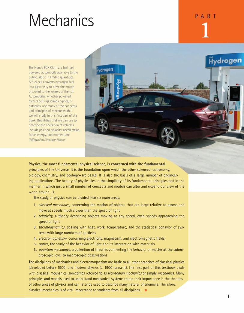
1
Mechanics p a r t
1the Honda FCX Clarity, a fuel-cell-powered automobile available to the public, albeit in limited quantities. a fuel cell converts hydrogen fuel into electricity to drive the motor attached to the wheels of the car. automobiles, whether powered by fuel cells, gasoline engines, or batteries, use many of the concepts and principles of mechanics that we will study in this first part of the book. Quantities that we can use to describe the operation of vehicles include position, velocity, acceleration, force, energy, and momentum. (PRNewsFoto/American Honda)
Physics, the most fundamental physical science, is concerned with the fundamental principles of the Universe. It is the foundation upon which the other sciences—astronomy, biology, chemistry, and geology—are based. It is also the basis of a large number of engineer-ing applications. the beauty of physics lies in the simplicity of its fundamental principles and in the manner in which just a small number of concepts and models can alter and expand our view of the world around us. the study of physics can be divided into six main areas:
1. classical mechanics, concerning the motion of objects that are large relative to atoms and move at speeds much slower than the speed of light
2. relativity, a theory describing objects moving at any speed, even speeds approaching the speed of light
3. thermodynamics, dealing with heat, work, temperature, and the statistical behavior of sys-tems with large numbers of particles
4. electromagnetism, concerning electricity, magnetism, and electromagnetic fields5. optics, the study of the behavior of light and its interaction with materials6. quantum mechanics, a collection of theories connecting the behavior of matter at the submi-
croscopic level to macroscopic observations
the disciplines of mechanics and electromagnetism are basic to all other branches of classical physics (developed before 1900) and modern physics (c. 1900–present). the first part of this textbook deals with classical mechanics, sometimes referred to as Newtonian mechanics or simply mechanics. Many principles and models used to understand mechanical systems retain their importance in the theories of other areas of physics and can later be used to describe many natural phenomena. therefore, classical mechanics is of vital importance to students from all disciplines. ■
2
Interactive content from this and other chapters may be assigned online in Enhanced Webassign.
c h a p t e r
11.1 Standards of Length, Mass,
and time
1.2 Matter and Model Building
1.3 Dimensional analysis
1.4 Conversion of Units
1.5 Estimates and Order-of-Magnitude Calculations
1.6 Significant Figures
physics and Measurement
Like all other sciences, physics is based on experimental observations and quantitative measurements. the main objectives of physics are to identify a limited number of funda-mental laws that govern natural phenomena and use them to develop theories that can pre-dict the results of future experiments. the fundamental laws used in developing theories are expressed in the language of mathematics, the tool that provides a bridge between theory and experiment. When there is a discrepancy between the prediction of a theory and experimental results, new or modified theories must be formulated to remove the discrepancy. Many times a theory is satisfactory only under limited conditions; a more general theory might be satisfactory without such limitations. For example, the laws of motion discovered by Isaac Newton (1642–1727) accurately describe the motion of objects moving at normal speeds but do not apply to objects moving at speeds comparable to the speed of light. In contrast, the special theory of relativity developed later by albert Einstein (1879–1955) gives the same results as Newton’s laws at low speeds but also correctly describes the motion of objects at speeds approaching the speed of light. Hence, Einstein’s special theory of relativity is a more general theory of motion than that formed from Newton’s laws. Classical physics includes the principles of classical mechanics, thermodynamics, optics, and electromagnetism developed before 1900. Important contributions to classical physics
Stonehenge, in southern England, was built thousands of years ago. Various theories have been proposed about its function, including a burial ground, a healing site, and a place for ancestor worship. One of the more intriguing theories suggests that Stonehenge was an observatory, allowing measurements of some of the quantities discussed in this chapter, such as position of objects in space and time intervals between repeating celestial events. (Stephen Inglis/Shutterstock.com)
1.1 Standards of Length, Mass, and time 3
were provided by Newton, who was also one of the originators of calculus as a mathemati-cal tool. Major developments in mechanics continued in the 18th century, but the fields of thermodynamics and electromagnetism were not developed until the latter part of the 19th century, principally because before that time the apparatus for controlled experiments in these disciplines was either too crude or unavailable. a major revolution in physics, usually referred to as modern physics, began near the end of the 19th century. Modern physics developed mainly because many physical phenomena could not be explained by classical physics. the two most important developments in this modern era were the theories of relativity and quantum mechanics. Einstein’s special the-ory of relativity not only correctly describes the motion of objects moving at speeds com-parable to the speed of light; it also completely modifies the traditional concepts of space, time, and energy. the theory also shows that the speed of light is the upper limit of the speed of an object and that mass and energy are related. Quantum mechanics was formu-lated by a number of distinguished scientists to provide descriptions of physical phenomena at the atomic level. Many practical devices have been developed using the principles of quantum mechanics. Scientists continually work at improving our understanding of fundamental laws. Numerous technological advances in recent times are the result of the efforts of many scientists, engineers, and technicians, such as unmanned planetary explorations, a vari-ety of developments and potential applications in nanotechnology, microcircuitry and high-speed computers, sophisticated imaging techniques used in scientific research and medicine, and several remarkable results in genetic engineering. the effects of such devel-opments and discoveries on our society have indeed been great, and it is very likely that future discoveries and developments will be exciting, challenging, and of great benefit to humanity.
1.1 Standards of Length, Mass, and TimeTo describe natural phenomena, we must make measurements of various aspects of nature. Each measurement is associated with a physical quantity, such as the length of an object. The laws of physics are expressed as mathematical relation-ships among physical quantities that we will introduce and discuss throughout the book. In mechanics, the three fundamental quantities are length, mass, and time. All other quantities in mechanics can be expressed in terms of these three. If we are to report the results of a measurement to someone who wishes to repro-duce this measurement, a standard must be defined. It would be meaningless if a visitor from another planet were to talk to us about a length of 8 “glitches” if we do not know the meaning of the unit glitch. On the other hand, if someone familiar with our system of measurement reports that a wall is 2 meters high and our unit of length is defined to be 1 meter, we know that the height of the wall is twice our basic length unit. Whatever is chosen as a standard must be readily accessible and must possess some property that can be measured reliably. Measurement standards used by different people in different places—throughout the Universe—must yield the same result. In addition, standards used for measurements must not change with time. In 1960, an international committee established a set of standards for the fun-damental quantities of science. It is called the SI (Système International), and its fundamental units of length, mass, and time are the meter, kilogram, and second, respectively. Other standards for SI fundamental units established by the commit-tee are those for temperature (the kelvin), electric current (the ampere), luminous intensity (the candela), and the amount of substance (the mole).
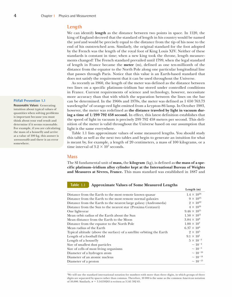
4 chapter 1 physics and Measurement
LengthWe can identify length as the distance between two points in space. In 1120, the king of England decreed that the standard of length in his country would be named the yard and would be precisely equal to the distance from the tip of his nose to the end of his outstretched arm. Similarly, the original standard for the foot adopted by the French was the length of the royal foot of King Louis XIV. Neither of these standards is constant in time; when a new king took the throne, length measure-ments changed! The French standard prevailed until 1799, when the legal standard of length in France became the meter (m), defined as one ten-millionth of the distance from the equator to the North Pole along one particular longitudinal line that passes through Paris. Notice that this value is an Earth-based standard that does not satisfy the requirement that it can be used throughout the Universe. As recently as 1960, the length of the meter was defined as the distance between two lines on a specific platinum–iridium bar stored under controlled conditions in France. Current requirements of science and technology, however, necessitate more accuracy than that with which the separation between the lines on the bar can be determined. In the 1960s and 1970s, the meter was defined as 1 650 763.73 wavelengths1 of orange-red light emitted from a krypton-86 lamp. In October 1983, however, the meter was redefined as the distance traveled by light in vacuum dur-ing a time of 1/299 792 458 second. In effect, this latest definition establishes that the speed of light in vacuum is precisely 299 792 458 meters per second. This defi-nition of the meter is valid throughout the Universe based on our assumption that light is the same everywhere. Table 1.1 lists approximate values of some measured lengths. You should study this table as well as the next two tables and begin to generate an intuition for what is meant by, for example, a length of 20 centimeters, a mass of 100 kilograms, or a time interval of 3.2 3 107 seconds.
MassThe SI fundamental unit of mass, the kilogram (kg), is defined as the mass of a spe-cific platinum–iridium alloy cylinder kept at the International Bureau of Weights and Measures at Sèvres, France. This mass standard was established in 1887 and
Pitfall Prevention 1.1Reasonable Values Generating intuition about typical values of quantities when solving problems is important because you must think about your end result and determine if it seems reasonable. For example, if you are calculating the mass of a housefly and arrive at a value of 100 kg, this answer is unreasonable and there is an error somewhere.
1We will use the standard international notation for numbers with more than three digits, in which groups of three digits are separated by spaces rather than commas. Therefore, 10 000 is the same as the common American notation of 10,000. Similarly, p 5 3.14159265 is written as 3.141 592 65.
Approximate Values of Some Measured Lengths Length (m)
Distance from the Earth to the most remote known quasar 1.4 3 1026
Distance from the Earth to the most remote normal galaxies 9 3 1025
Distance from the Earth to the nearest large galaxy (Andromeda) 2 3 1022
Distance from the Sun to the nearest star (Proxima Centauri) 4 3 1016
One light-year 9.46 3 1015
Mean orbit radius of the Earth about the Sun 1.50 3 1011
Mean distance from the Earth to the Moon 3.84 3 108
Distance from the equator to the North Pole 1.00 3 107
Mean radius of the Earth 6.37 3 106
Typical altitude (above the surface) of a satellite orbiting the Earth 2 3 105
Length of a football field 9.1 3 101
Length of a housefly 5 3 1023
Size of smallest dust particles , 1024
Size of cells of most living organisms , 1025
Diameter of a hydrogen atom , 10210
Diameter of an atomic nucleus , 10214
Diameter of a proton , 10215
Table 1.1
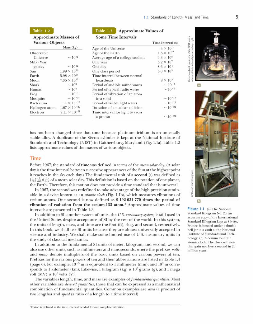
1.1 Standards of Length, Mass, and time 5
has not been changed since that time because platinum–iridium is an unusually stable alloy. A duplicate of the Sèvres cylinder is kept at the National Institute of Standards and Technology (NIST) in Gaithersburg, Maryland (Fig. 1.1a). Table 1.2 lists approximate values of the masses of various objects.
TimeBefore 1967, the standard of time was defined in terms of the mean solar day. (A solar day is the time interval between successive appearances of the Sun at the highest point it reaches in the sky each day.) The fundamental unit of a second (s) was defined as 1 1
60 2 1 160 2 1 1
24 2 of a mean solar day. This definition is based on the rotation of one planet, the Earth. Therefore, this motion does not provide a time standard that is universal. In 1967, the second was redefined to take advantage of the high precision attain-able in a device known as an atomic clock (Fig. 1.1b), which measures vibrations of cesium atoms. One second is now defined as 9 192 631 770 times the period of vibration of radiation from the cesium-133 atom.2 Approximate values of time intervals are presented in Table 1.3. In addition to SI, another system of units, the U.S. customary system, is still used in the United States despite acceptance of SI by the rest of the world. In this system, the units of length, mass, and time are the foot (ft), slug, and second, respectively. In this book, we shall use SI units because they are almost universally accepted in science and industry. We shall make some limited use of U.S. customary units in the study of classical mechanics. In addition to the fundamental SI units of meter, kilogram, and second, we can also use other units, such as millimeters and nanoseconds, where the prefixes milli- and nano- denote multipliers of the basic units based on various powers of ten. Prefixes for the various powers of ten and their abbreviations are listed in Table 1.4 (page 6). For example, 1023 m is equivalent to 1 millimeter (mm), and 103 m corre-sponds to 1 kilometer (km). Likewise, 1 kilogram (kg) is 103 grams (g), and 1 mega volt (MV) is 106 volts (V). The variables length, time, and mass are examples of fundamental quantities. Most other variables are derived quantities, those that can be expressed as a mathematical combination of fundamental quantities. Common examples are area (a product of two lengths) and speed (a ratio of a length to a time interval).
2Period is defined as the time interval needed for one complete vibration.
Approximate Masses of Various Objects
Mass (kg)
Observable Universe , 1052
Milky Way galaxy , 1042
Sun 1.99 3 1030
Earth 5.98 3 1024
Moon 7.36 3 1022
Shark , 103
Human , 102
Frog , 1021
Mosquito , 1025
Bacterium , 1 3 10215
Hydrogen atom 1.67 3 10227
Electron 9.11 3 10231
Table 1.2 Approximate Values of Some Time Intervals
Time Interval (s)
Age of the Universe 4 3 1017
Age of the Earth 1.3 3 1017
Average age of a college student 6.3 3 108
One year 3.2 3 107
One day 8.6 3 104
One class period 3.0 3 103
Time interval between normal heartbeats 8 3 1021
Period of audible sound waves , 1023
Period of typical radio waves , 1026
Period of vibration of an atom in a solid , 10213
Period of visible light waves , 10215
Duration of a nuclear collision , 10222
Time interval for light to cross a proton , 10224
Table 1.3
Figure 1.1 (a) The National Standard Kilogram No. 20, an accurate copy of the International Standard Kilogram kept at Sèvres, France, is housed under a double bell jar in a vault at the National Institute of Standards and Tech-nology. (b) A cesium fountain atomic clock. The clock will nei-ther gain nor lose a second in 20 million years.
a
Repr
oduc
ed w
ith p
erm
issi
on o
f the
BIP
M, w
hich
re
tain
s fu
ll in
tern
atio
nally
pro
tect
ed c
opyr
ight
.
b
AP
Phot
o/Fo
cke
Stra
ngm
ann
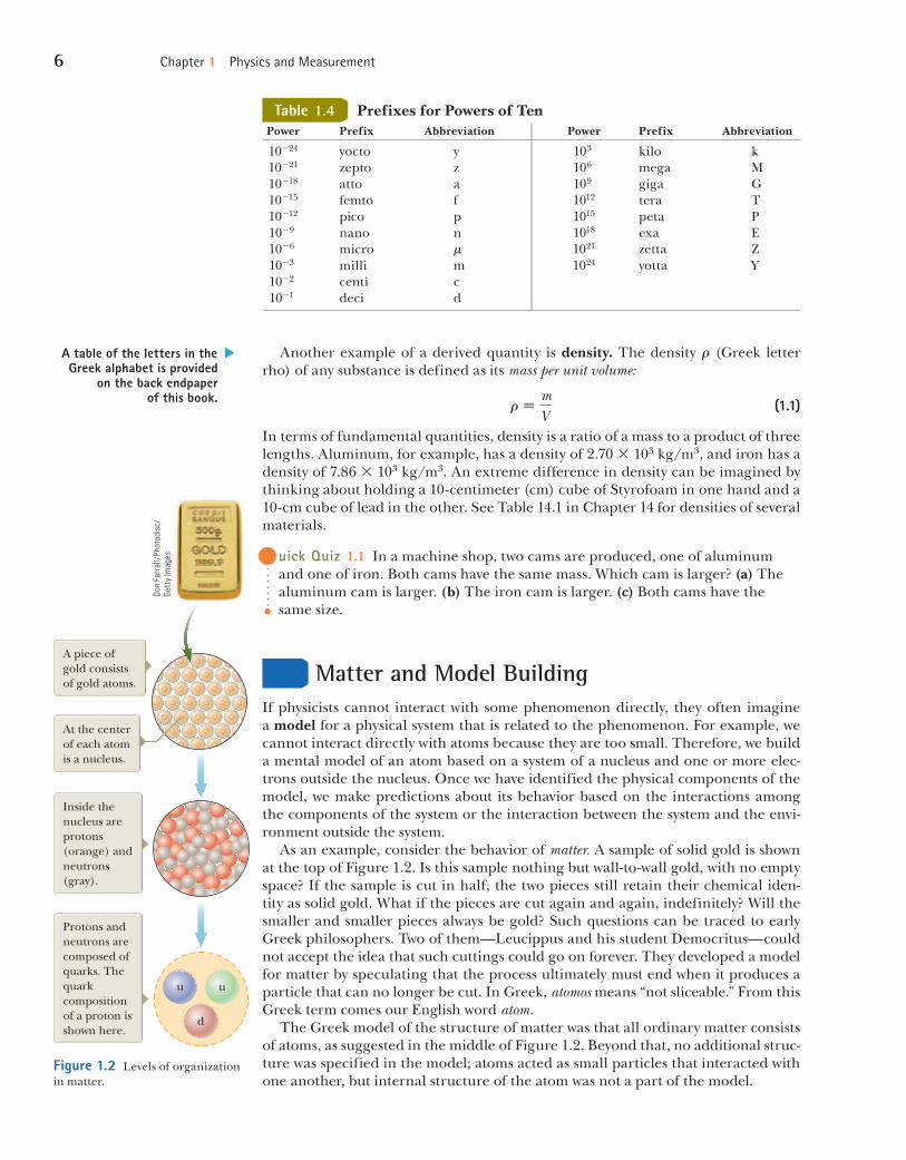
6 chapter 1 physics and Measurement
Another example of a derived quantity is density. The density r (Greek letter rho) of any substance is defined as its mass per unit volume:
r ;mV
(1.1)
In terms of fundamental quantities, density is a ratio of a mass to a product of three lengths. Aluminum, for example, has a density of 2.70 3 103 kg/m3, and iron has a density of 7.86 3 103 kg/m3. An extreme difference in density can be imagined by thinking about holding a 10-centimeter (cm) cube of Styrofoam in one hand and a 10-cm cube of lead in the other. See Table 14.1 in Chapter 14 for densities of several materials.
Q uick Quiz 1.1 In a machine shop, two cams are produced, one of aluminum and one of iron. Both cams have the same mass. Which cam is larger? (a) The aluminum cam is larger. (b) The iron cam is larger. (c) Both cams have the same size.
1.2 Matter and Model BuildingIf physicists cannot interact with some phenomenon directly, they often imagine a model for a physical system that is related to the phenomenon. For example, we cannot interact directly with atoms because they are too small. Therefore, we build a mental model of an atom based on a system of a nucleus and one or more elec-trons outside the nucleus. Once we have identified the physical components of the model, we make predictions about its behavior based on the interactions among the components of the system or the interaction between the system and the envi-ronment outside the system. As an example, consider the behavior of matter. A sample of solid gold is shown at the top of Figure 1.2. Is this sample nothing but wall-to-wall gold, with no empty space? If the sample is cut in half, the two pieces still retain their chemical iden-tity as solid gold. What if the pieces are cut again and again, indefinitely? Will the smaller and smaller pieces always be gold? Such questions can be traced to early Greek philosophers. Two of them—Leucippus and his student Democritus—could not accept the idea that such cuttings could go on forever. They developed a model for matter by speculating that the process ultimately must end when it produces a particle that can no longer be cut. In Greek, atomos means “not sliceable.” From this Greek term comes our English word atom. The Greek model of the structure of matter was that all ordinary matter consists of atoms, as suggested in the middle of Figure 1.2. Beyond that, no additional struc-ture was specified in the model; atoms acted as small particles that interacted with one another, but internal structure of the atom was not a part of the model.
A table of the letters in the Greek alphabet is provided
on the back endpaper of this book.
Prefixes for Powers of Ten Power Prefix Abbreviation Power Prefix Abbreviation
10224 yocto y 103 kilo k 10221 zepto z 106 mega M 10218 atto a 109 giga G 10215 femto f 1012 tera T 10212 pico p 1015 peta P 1029 nano n 1018 exa E 1026 micro m 1021 zetta Z 1023 milli m 1024 yotta Y 1022 centi c 1021 deci d
Table 1.4
Figure 1.2 Levels of organization in matter.
A piece of gold consists of gold atoms.
At the center of each atom is a nucleus.
Inside the nucleus are protons (orange) and neutrons (gray).
Protons and neutrons are composed of quarks. The quark composition of a proton is shown here.
p
u u
d
Don
Farr
all/
Phot
odis
c/Ge
tty
Imag
es
1.3 Dimensional analysis 7
In 1897, J. J. Thomson identified the electron as a charged particle and as a constituent of the atom. This led to the first atomic model that contained internal structure. We shall discuss this model in Chapter 42. Following the discovery of the nucleus in 1911, an atomic model was developed in which each atom is made up of electrons surrounding a central nucleus. A nucleus of gold is shown in Figure 1.2. This model leads, however, to a new question: Does the nucleus have structure? That is, is the nucleus a single particle or a collection of particles? By the early 1930s, a model evolved that described two basic entities in the nucleus: protons and neutrons. The proton carries a positive electric charge, and a specific chemical element is identified by the number of protons in its nucleus. This number is called the atomic number of the element. For instance, the nucleus of a hydrogen atom contains one proton (so the atomic number of hydrogen is 1), the nucleus of a helium atom contains two protons (atomic number 2), and the nucleus of a uranium atom contains 92 protons (atomic number 92). In addition to atomic number, a second number—mass number, defined as the number of protons plus neutrons in a nucleus—characterizes atoms. The atomic number of a specific ele-ment never varies (i.e., the number of protons does not vary), but the mass number can vary (i.e., the number of neutrons varies). Is that, however, where the process of breaking down stops? Protons, neutrons, and a host of other exotic particles are now known to be composed of six different varieties of particles called quarks, which have been given the names of up, down, strange, charmed, bottom, and top. The up, charmed, and top quarks have electric charges of 12
3 that of the proton, whereas the down, strange, and bottom quarks have charges of 21
3 that of the proton. The proton consists of two up quarks and one down quark as shown at the bottom of Figure 1.2 and labeled u and d. This structure predicts the correct charge for the proton. Likewise, the neutron consists of two down quarks and one up quark, giving a net charge of zero. You should develop a process of building models as you study physics. In this study, you will be challenged with many mathematical problems to solve. One of the most important problem-solving techniques is to build a model for the prob-lem: identify a system of physical components for the problem and make predic-tions of the behavior of the system based on the interactions among its components or the interaction between the system and its surrounding environment.
1.3 Dimensional AnalysisIn physics, the word dimension denotes the physical nature of a quantity. The dis-tance between two points, for example, can be measured in feet, meters, or fur-longs, which are all different ways of expressing the dimension of length. The symbols we use in this book to specify the dimensions of length, mass, and time are L, M, and T, respectively.3 We shall often use brackets [ ] to denote the dimensions of a physical quantity. For example, the symbol we use for speed in this book is v, and in our notation, the dimensions of speed are written [v] 5 L/T. As another example, the dimensions of area A are [A] 5 L2. The dimensions and units of area, volume, speed, and acceleration are listed in Table 1.5. The dimensions of other quantities, such as force and energy, will be described as they are introduced in the text.
3The dimensions of a quantity will be symbolized by a capitalized, nonitalic letter such as L or T. The algebraic symbol for the quantity itself will be an italicized letter such as L for the length of an object or t for time.
Table 1.5 Dimensions and Units of Four Derived Quantities
Quantity Area (A) Volume (V ) Speed (v) Acceleration (a)
Dimensions L2 L3 L/T L/T2
SI units m2 m3 m/s m/s2
U.S. customary units ft2 ft3 ft/s ft/s2
8 chapter 1 physics and Measurement
In many situations, you may have to check a specific equation to see if it matches your expectations. A useful procedure for doing that, called dimensional analysis, can be used because dimensions can be treated as algebraic quantities. For exam-ple, quantities can be added or subtracted only if they have the same dimensions. Furthermore, the terms on both sides of an equation must have the same dimen-sions. By following these simple rules, you can use dimensional analysis to deter-mine whether an expression has the correct form. Any relationship can be correct only if the dimensions on both sides of the equation are the same. To illustrate this procedure, suppose you are interested in an equation for the position x of a car at a time t if the car starts from rest at x 5 0 and moves with con-stant acceleration a. The correct expression for this situation is x 5 1
2 at 2 as we show in Chapter 2. The quantity x on the left side has the dimension of length. For the equation to be dimensionally correct, the quantity on the right side must also have the dimension of length. We can perform a dimensional check by substituting the dimensions for acceleration, L/T2 (Table 1.5), and time, T, into the equation. That is, the dimensional form of the equation x 5 1
2 at 2 is
L 5LT2
# T2 5 L
The dimensions of time cancel as shown, leaving the dimension of length on the right-hand side to match that on the left. A more general procedure using dimensional analysis is to set up an expression of the form
x ~ ant m
where n and m are exponents that must be determined and the symbol ~ indicates a proportionality. This relationship is correct only if the dimensions of both sides are the same. Because the dimension of the left side is length, the dimension of the right side must also be length. That is,
3ant m 4 5 L 5 L1T0
Because the dimensions of acceleration are L/T2 and the dimension of time is T, we have
1L/T2 2nTm 5 L1T0 S 1LnTm22n 2 5 L1T0
The exponents of L and T must be the same on both sides of the equation. From the exponents of L, we see immediately that n 5 1. From the exponents of T, we see that m 2 2n 5 0, which, once we substitute for n, gives us m 5 2. Returning to our original expression x ~ ant m, we conclude that x ~ at2 .
Q uick Quiz 1.2 True or False: Dimensional analysis can give you the numerical value of constants of proportionality that may appear in an algebraic expression.
Pitfall Prevention 1.2Symbols for Quantities Some quantities have a small number of symbols that represent them. For example, the symbol for time is almost always t. Other quanti-ties might have various symbols depending on the usage. Length may be described with symbols such as x, y, and z (for position); r (for radius); a, b, and c (for the legs of a right triangle); , (for the length of an object); d (for a dis-tance); h (for a height); and so forth.
Identify the dimensions of v from Table 1.5: 3v 4 5LT
Example 1.1 Analysis of an Equation
Show that the expression v 5 at, where v represents speed, a acceleration, and t an instant of time, is dimensionally correct.
S o L u t i o n
1.4 conversion of Units 9
1.4 Conversion of UnitsSometimes it is necessary to convert units from one measurement system to another or convert within a system (for example, from kilometers to meters). Conversion factors between SI and U.S. customary units of length are as follows:
1 mile 5 1 609 m 5 1.609 km 1 ft 5 0.304 8 m 5 30.48 cm 1 m 5 39.37 in. 5 3.281 ft 1 in. 5 0.025 4 m 5 2.54 cm (exactly)
A more complete list of conversion factors can be found in Appendix A. Like dimensions, units can be treated as algebraic quantities that can can-cel each other. For example, suppose we wish to convert 15.0 in. to centimeters. Because 1 in. is defined as exactly 2.54 cm, we find that
15.0 in. 5 115.0 in. 2 a2.54 cm1 in.
b 5 38.1 cm
where the ratio in parentheses is equal to 1. We express 1 as 2.54 cm/1 in. (rather than 1 in./2.54 cm) so that the unit “inch” in the denominator cancels with the unit in the original quantity. The remaining unit is the centimeter, our desired result.
1.4 Pitfall Prevention 1.3Always include units When per-forming calculations with numeri-cal values, include the units for every quantity and carry the units through the entire calculation. Avoid the temptation to drop the units early and then attach the expected units once you have an answer. By including the units in every step, you can detect errors if the units for the answer turn out to be incorrect.
Write an expression for a with a dimensionless constant of proportionality k:
a 5 krnvm
Substitute the dimensions of a, r, and v:LT2 5 Ln aL
Tb
m
5Ln1m
Tm
Equate the exponents of L and T so that the dimen-sional equation is balanced:
n 1 m 5 1 and m 5 2
Solve the two equations for n: n 5 21
Write the acceleration expression: a 5 kr21 v 2 5 k v 2
r
In Section 4.4 on uniform circular motion, we show that k 5 1 if a consistent set of units is used. The constant k would not equal 1 if, for example, v were in km/h and you wanted a in m/s2 .
Example 1.2 Analysis of a Power Law
Suppose we are told that the acceleration a of a particle moving with uniform speed v in a circle of radius r is propor-tional to some power of r, say rn, and some power of v, say v m. Determine the values of n and m and write the simplest form of an equation for the acceleration.
S o L u t i o n
Identify the dimensions of a from Table 1.5 and multiply by the dimensions of t :
3at 4 5LT2 T 5
LT
Therefore, v 5 at is dimensionally correct because we have the same dimensions on both sides. (If the expression were given as v 5 at2, it would be dimensionally incorrect. Try it and see!)
▸ 1.1 c o n t i n u e d
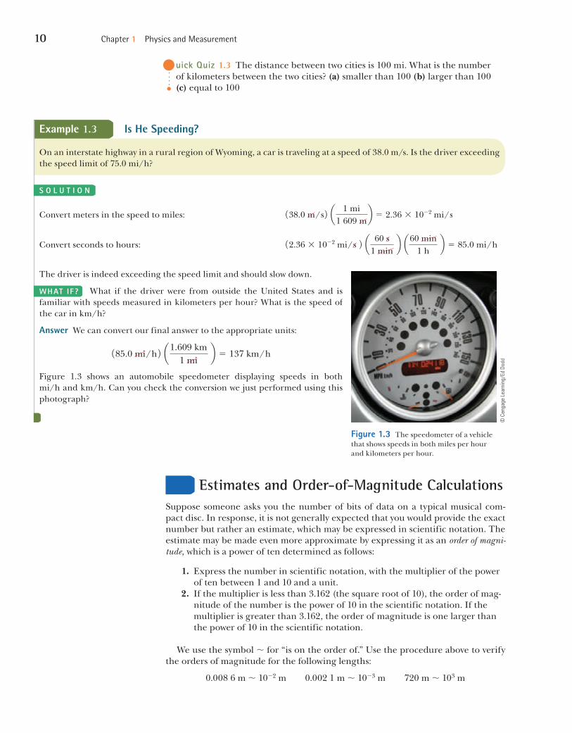
10 chapter 1 physics and Measurement
1.5 Estimates and Order-of-Magnitude CalculationsSuppose someone asks you the number of bits of data on a typical musical com-pact disc. In response, it is not generally expected that you would provide the exact number but rather an estimate, which may be expressed in scientific notation. The estimate may be made even more approximate by expressing it as an order of magni-tude, which is a power of ten determined as follows:
1. Express the number in scientific notation, with the multiplier of the power of ten between 1 and 10 and a unit.
2. If the multiplier is less than 3.162 (the square root of 10), the order of mag-nitude of the number is the power of 10 in the scientific notation. If the multiplier is greater than 3.162, the order of magnitude is one larger than the power of 10 in the scientific notation.
We use the symbol , for “is on the order of.” Use the procedure above to verify the orders of magnitude for the following lengths:
0.008 6 m , 1022 m 0.002 1 m , 1023 m 720 m , 103 m
Q uick Quiz 1.3 The distance between two cities is 100 mi. What is the number of kilometers between the two cities? (a) smaller than 100 (b) larger than 100 (c) equal to 100
Convert meters in the speed to miles: 138.0 m/s 2 a 1 mi1 609 m
b 5 2.36 3 1022 mi/s
Convert seconds to hours: 12.36 3 1022 mi/s 2 a 60 s1 min
b a60 min1 h
b 5 85.0 mi/h
The driver is indeed exceeding the speed limit and should slow down.
What if the driver were from outside the United States and is familiar with speeds measured in kilometers per hour? What is the speed of the car in km/h?
Answer We can convert our final answer to the appropriate units:
185.0 mi/h 2 a1.609 km1 mi
b 5 137 km/h
Figure 1.3 shows an automobile speedometer displaying speeds in both mi/h and km/h. Can you check the conversion we just performed using this photograph?
WhAt iF ?
Figure 1.3 The speedometer of a vehicle that shows speeds in both miles per hour and kilometers per hour.
© C
enga
ge L
earn
ing/
Ed D
odd
Example 1.3 Is He Speeding?
On an interstate highway in a rural region of Wyoming, a car is traveling at a speed of 38.0 m/s. Is the driver exceeding the speed limit of 75.0 mi/h?
S o L u t i o n
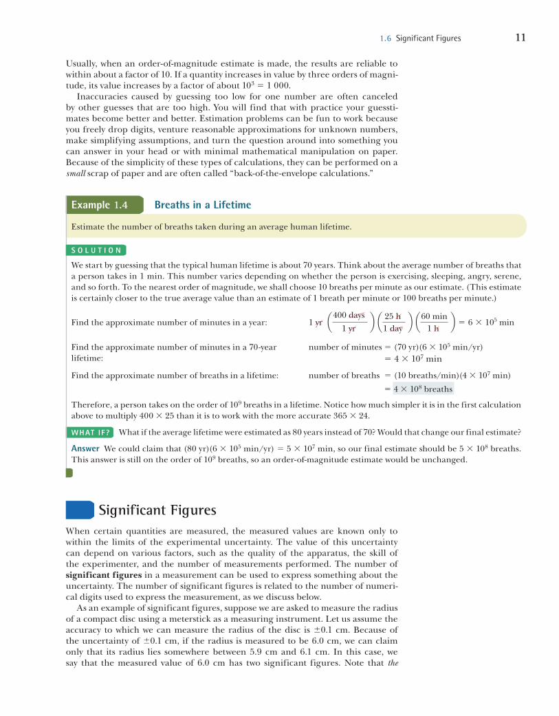
1.6 Significant Figures 11
Usually, when an order-of-magnitude estimate is made, the results are reliable to within about a factor of 10. If a quantity increases in value by three orders of magni-tude, its value increases by a factor of about 103 5 1 000. Inaccuracies caused by guessing too low for one number are often canceled by other guesses that are too high. You will find that with practice your guessti-mates become better and better. Estimation problems can be fun to work because you freely drop digits, venture reasonable approximations for unknown numbers, make simplifying assumptions, and turn the question around into something you can answer in your head or with minimal mathematical manipulation on paper. Because of the simplicity of these types of calculations, they can be performed on a small scrap of paper and are often called “back-of-the-envelope calculations.”
1.6 Significant FiguresWhen certain quantities are measured, the measured values are known only to within the limits of the experimental uncertainty. The value of this uncertainty can depend on various factors, such as the quality of the apparatus, the skill of the experimenter, and the number of measurements performed. The number of significant figures in a measurement can be used to express something about the uncertainty. The number of significant figures is related to the number of numeri-cal digits used to express the measurement, as we discuss below. As an example of significant figures, suppose we are asked to measure the radius of a compact disc using a meterstick as a measuring instrument. Let us assume the accuracy to which we can measure the radius of the disc is 60.1 cm. Because of the uncertainty of 60.1 cm, if the radius is measured to be 6.0 cm, we can claim only that its radius lies somewhere between 5.9 cm and 6.1 cm. In this case, we say that the measured value of 6.0 cm has two significant figures. Note that the
1 yr a400 days
1 yr b a 25 h
1 day b a60 min
1 h b 5 6 3 105 minFind the approximate number of minutes in a year:
Find the approximate number of minutes in a 70-year lifetime:
number of minutes 5 (70 yr)(6 3 105 min/yr) 5 4 3 107 min
Find the approximate number of breaths in a lifetime: number of breaths 5 (10 breaths/min)(4 3 107 min)
5 4 3 108 breaths
Therefore, a person takes on the order of 109 breaths in a lifetime. Notice how much simpler it is in the first calculation above to multiply 400 3 25 than it is to work with the more accurate 365 3 24.
What if the average lifetime were estimated as 80 years instead of 70? Would that change our final estimate?
Answer We could claim that (80 yr)(6 3 105 min/yr) 5 5 3 107 min, so our final estimate should be 5 3 108 breaths. This answer is still on the order of 109 breaths, so an order-of-magnitude estimate would be unchanged.
WhAt iF ?
Example 1.4 Breaths in a Lifetime
Estimate the number of breaths taken during an average human lifetime.
We start by guessing that the typical human lifetime is about 70 years. Think about the average number of breaths that a person takes in 1 min. This number varies depending on whether the person is exercising, sleeping, angry, serene, and so forth. To the nearest order of magnitude, we shall choose 10 breaths per minute as our estimate. (This estimate is certainly closer to the true average value than an estimate of 1 breath per minute or 100 breaths per minute.)
S o L u t i o n
12 chapter 1 physics and Measurement
significant figures include the first estimated digit. Therefore, we could write the radius as (6.0 6 0.1) cm. Zeros may or may not be significant figures. Those used to position the decimal point in such numbers as 0.03 and 0.007 5 are not significant. Therefore, there are one and two significant figures, respectively, in these two values. When the zeros come after other digits, however, there is the possibility of misinterpretation. For example, suppose the mass of an object is given as 1 500 g. This value is ambigu-ous because we do not know whether the last two zeros are being used to locate the decimal point or whether they represent significant figures in the measurement. To remove this ambiguity, it is common to use scientific notation to indicate the number of significant figures. In this case, we would express the mass as 1.5 3 103 g if there are two significant figures in the measured value, 1.50 3 103 g if there are three sig-nificant figures, and 1.500 3 103 g if there are four. The same rule holds for numbers less than 1, so 2.3 3 1024 has two significant figures (and therefore could be written 0.000 23) and 2.30 3 1024 has three significant figures (also written as 0.000 230). In problem solving, we often combine quantities mathematically through mul-tiplication, division, addition, subtraction, and so forth. When doing so, you must make sure that the result has the appropriate number of significant figures. A good rule of thumb to use in determining the number of significant figures that can be claimed in a multiplication or a division is as follows:
When multiplying several quantities, the number of significant figures in the final answer is the same as the number of significant figures in the quantity hav-ing the smallest number of significant figures. The same rule applies to division.
Let’s apply this rule to find the area of the compact disc whose radius we mea-sured above. Using the equation for the area of a circle,
A 5 pr 2 5 p 16.0 cm 2 2 5 1.1 3 102 cm2
If you perform this calculation on your calculator, you will likely see 113.097 335 5. It should be clear that you don’t want to keep all of these digits, but you might be tempted to report the result as 113 cm2. This result is not justified because it has three significant figures, whereas the radius only has two. Therefore, we must report the result with only two significant figures as shown above. For addition and subtraction, you must consider the number of decimal places when you are determining how many significant figures to report:
When numbers are added or subtracted, the number of decimal places in the result should equal the smallest number of decimal places of any term in the sum or difference.
As an example of this rule, consider the sum
23.2 1 5.174 5 28.4
Notice that we do not report the answer as 28.374 because the lowest number of decimal places is one, for 23.2. Therefore, our answer must have only one decimal place. The rule for addition and subtraction can often result in answers that have a dif-ferent number of significant figures than the quantities with which you start. For example, consider these operations that satisfy the rule:
1.000 1 1 0.000 3 5 1.000 4
1.002 2 0.998 5 0.004
In the first example, the result has five significant figures even though one of the terms, 0.000 3, has only one significant figure. Similarly, in the second calcu-lation, the result has only one significant figure even though the numbers being subtracted have four and three, respectively.
Pitfall Prevention 1.4Read Carefully Notice that the rule for addition and subtraction is different from that for multipli-cation and division. For addition and subtraction, the important consideration is the number of decimal places, not the number of significant figures.
Summary 13
In this book, most of the numerical examples and end-of-chapter problems will yield answers having three significant figures. When carrying out estima-tion calculations, we shall typically work with a single significant figure.
If the number of significant figures in the result of a calculation must be reduced, there is a general rule for rounding numbers: the last digit retained is increased by 1 if the last digit dropped is greater than 5. (For example, 1.346 becomes 1.35.) If the last digit dropped is less than 5, the last digit retained remains as it is. (For example, 1.343 becomes 1.34.) If the last digit dropped is equal to 5, the remaining digit should be rounded to the nearest even number. (This rule helps avoid accu-mulation of errors in long arithmetic processes.) A technique for avoiding error accumulation is to delay the rounding of num-bers in a long calculation until you have the final result. Wait until you are ready to copy the final answer from your calculator before rounding to the correct number of significant figures. In this book, we display numerical values rounded off to two or three significant figures. This occasionally makes some mathematical manipula-tions look odd or incorrect. For instance, looking ahead to Example 3.5 on page 69, you will see the operation 217.7 km 1 34.6 km 5 17.0 km. This looks like an incor-rect subtraction, but that is only because we have rounded the numbers 17.7 km and 34.6 km for display. If all digits in these two intermediate numbers are retained and the rounding is only performed on the final number, the correct three-digit result of 17.0 km is obtained.
WW Significant figure guidelines used in this book
Pitfall Prevention 1.5Symbolic Solutions When solving problems, it is very useful to per-form the solution completely in algebraic form and wait until the very end to enter numerical values into the final symbolic expres-sion. This method will save many calculator keystrokes, especially if some quantities cancel so that you never have to enter their values into your calculator! In addition, you will only need to round once, on the final result.
Summary
Definitions
The three fundamental physical quantities of mechanics are length, mass, and time, which in the SI system have the units meter (m), kilogram (kg), and second (s), respectively. These fundamental quantities cannot be defined in terms of more basic quantities.
The density of a substance is defined as its mass per unit volume:
r ;mV
(1.1)
Example 1.5 Installing a Carpet
A carpet is to be installed in a rectangular room whose length is measured to be 12.71 m and whose width is measured to be 3.46 m. Find the area of the room.
If you multiply 12.71 m by 3.46 m on your calculator, you will see an answer of 43.976 6 m2. How many of these num-bers should you claim? Our rule of thumb for multiplication tells us that you can claim only the number of significant figures in your answer as are present in the measured quantity having the lowest number of significant figures. In this example, the lowest number of significant figures is three in 3.46 m, so we should express our final answer as 44.0 m2.
S o L u t i o n
continued
14 chapter 1 physics and Measurement
1. One student uses a meterstick to measure the thick-ness of a textbook and obtains 4.3 cm 6 0.1 cm. Other students measure the thickness with vernier calipers and obtain four different measurements: (a) 4.32 cm 6 0.01 cm, (b) 4.31 cm 6 0.01 cm, (c) 4.24 cm 6 0.01 cm, and (d) 4.43 cm 6 0.01 cm. Which of these four mea-surements, if any, agree with that obtained by the first student?
2. A house is advertised as having 1 420 square feet under its roof. What is its area in square meters? (a) 4 660 m2 (b) 432 m2 (c) 158 m2 (d) 132 m2 (e) 40.2 m2
3. Answer each question yes or no. Must two quantities have the same dimensions (a) if you are adding them? (b) If you are multiplying them? (c) If you are subtract-ing them? (d) If you are dividing them? (e) If you are equating them?
4. The price of gasoline at a particular station is 1.5 euros per liter. An American student can use 33 euros to buy gasoline. Knowing that 4 quarts make a gallon and that 1 liter is close to 1 quart, she quickly reasons that she can buy how many gallons of gasoline? (a) less than 1 gallon (b) about 5 gallons (c) about 8 gallons (d) more than 10 gallons
5. Rank the following five quantities in order from the largest to the smallest. If two of the quantities are equal,
give them equal rank in your list. (a) 0.032 kg (b) 15 g (c) 2.7 3 105 mg (d) 4.1 3 1028 Gg (e) 2.7 3 108 mg
6. What is the sum of the measured values 21.4 s 1 15 s 1 17.17 s 1 4.00 3 s? (a) 57.573 s (b) 57.57 s (c) 57.6 s (d) 58 s (e) 60 s
7. Which of the following is the best estimate for the mass of all the people living on the Earth? (a) 2 3 108 kg (b) 1 3 109 kg (c) 2 3 1010 kg (d) 3 3 1011 kg (e) 4 3 1012 kg
8. (a) If an equation is dimensionally correct, does that mean that the equation must be true? (b) If an equa-tion is not dimensionally correct, does that mean that the equation cannot be true?
9. Newton’s second law of motion (Chapter 5) says that the mass of an object times its acceleration is equal to the net force on the object. Which of the following gives the correct units for force? (a) kg ? m/s2 (b) kg ? m2/s2 (c) kg/m ? s2 (d) kg ? m2/s (e) none of those answers
10. A calculator displays a result as 1.365 248 0 3 107 kg. The estimated uncertainty in the result is 62%. How many digits should be included as significant when the result is written down? (a) zero (b) one (c) two (d) three (e) four
Objective Questions 1. denotes answer available in Student Solutions Manual/Study Guide
Conceptual Questions 1. denotes answer available in Student Solutions Manual/Study Guide
1. Suppose the three fundamental standards of the met-ric system were length, density, and time rather than length, mass, and time. The standard of density in this system is to be defined as that of water. What consid-erations about water would you need to address to make sure that the standard of density is as accurate as possible?
2. Why is the metric system of units considered superior to most other systems of units?
3. What natural phenomena could serve as alternative time standards?
4. Express the following quantities using the prefixes given in Table 1.4. (a) 3 3 1024 m (b) 5 3 1025 s (c) 72 3 102 g
Concepts and Principles
When you compute a result from several measured numbers, each of which has a certain accuracy, you should give the result with the correct number of sig-nificant figures.
When multiplying several quantities, the number of significant figures in the final answer is the same as the number of significant figures in the quantity having the smallest number of significant figures. The same rule applies to division.
When numbers are added or subtracted, the number of decimal places in the result should equal the small-est number of decimal places of any term in the sum or difference.
The method of dimensional analysis is very power-ful in solving physics problems. Dimensions can be treated as algebraic quantities. By making estimates and performing order-of-magnitude calculations, you should be able to approximate the answer to a prob-lem when there is not enough information available to specify an exact solution completely.


![[Serway] Physics for Scientists and Engineers - So(BookFi.org)](https://static.fdocuments.in/doc/165x107/55cf852c550346484b8b7761/serway-physics-for-scientists-and-engineers-sobookfiorg.jpg)


