A Matlab Problem-Solving Environment forNonlinear Systems Education in

Mathematics, Physics and Engineering

Akemi G\’alvez TomidaDepartment of Applied Mathematics and Comp. Sciences

University of Cantabria, Avda. de los Castross/n, E-39005, Santander, Spain

galveza@unican.es

AbstractCurrently, European countries are in the process of rethinking their Higher Edu-

cation systems due to harmonization efforts initiated by Bologna’s declaration. Thisscenario of reforms demands a completely new approach to the instructional process.A major issue in this context is the development of better, updated educationaltools and materials specially adapted to the topics under study. This work reflectsauthor’s experience in developing a problem-solving environment designed for a firstcourse on nonlinear systems for undergraduate students of Mathematics, Physicsand Engineering. In this paper the architecture of this computer system along witha description of its main functionalities are briefly reported.

1 IntroductionBologna’s declaration - seen today as the well-known synonym for the whole processof reformation in the area of higher education-was signed in 1999 by 29 Europeancountries with the objective to create “a European space for higher education in orderto enhance the employability and mobility of citizens and to increase the intemationalcompetitiveness of European higher education” [1]. Its upmost goal is the commitmentfreely taken by each signatory country to reform its own higher education system inorder to create overall convergence at European level. This process encompasses theadoption of a common framework of readable and comparable degrees as well as theintroduction of undergraduate and postgraduate levels in all countries along with ECTS(European Credit Transfer System) credit systems to ensure a smooth transition fromone country’s system to another one, thus enforcing free mobility of students, teachersand administrators among the European countries.

Unquestionably, Bologna’s declaration opened the door to a completely new scenariofor higher education in Europe. Nowadays, the European countries are in the midst ofthe process of restructuring their higher education system in order to fulfill the objectivesof the declaration. At this time, the developments focus especially on academic aspects,

数理解析研究所講究録第 1624巻 2009年 129-143 129

such as the definition of the new curricula and grading systeins. However, the upcomingchanges go far beyond these structural changes, as the personal development of studentsand teachers is also at the root of this new concept of education. For instance, studentsin this new model are no longer passive actors of the learning process. On the contrary,Bologna’s declaration emphasizes the concept of self-learning so that students are gettingmore and more involved in their own learning.

An important issue in this process is to provide students with a good collection ofscholar materials that enable them to accomplish the learning process by themselves.During the last few years, the author has been involved in the development of computersoftware for a first course on nonlinear systems for undergraduate students of Mathemat-ics, Physics and Engineering. As a result, a new Matlab problem-solving environmentdesigned to attain the demands of this new situation has been created from scratch. Inthis paper the architecture of this computer system along with a description of its mainfunctionalities are briefly reported.

2 Nonlinear (Chaotic) SystemsThe analysis of chaotic dynamical systems is one of the most challenging tasks in Com-putational Science. Because the chaotic systems are essentially nonlinear, their behavioris much more complicated than that of linear systems. In fact, even the simplest chaoticsystems exhibit a bulk of different behaviors that can only be $f\iota illy$ analyzed with thehelp of powerful hardware and software resources.

The range of different phenomena associated with the nonlinear systems is extremelyvaried. Chaos can be found in almost any field, ranging from chemical reactions to elec-tronic circuits and lasers [2, 11], meteorology [16], ecology [18], etc. Nonlinearity appearsin both discrete and continuous systems, which are described by iterated functions anddifferential equations, respectively [15, 19]. That means that the accurate analysis ofsuch chaotic systems requires specialized mathematical tools and techniques, designedto account for the kind of system involved. This challenging issue has motivated an in-tensive development of programs and packages aimed at analyzing the range of differentphenomena associated with the chaotic systems.

Among these programs and packages, those based on computer algebra systems (CAS)are receiving increasing attention during the last few years. Recent examples can befound, for instance, in [3, 4, 5, 6, 8] for Matlab, in [7, 9, 10, 12, 13, 14, 21] for Mathematicaand in [22] for Maple, to mention just a few examples. In addition to their outstandingsymbolic features, the CAS also include optimized numerical routines, nice graphicalcapabilities and- in a few cases such as in Matlab- the possibility to generate appealingGUIs (Graphical User Interfaces).

In this paper, we describe a problem-solving environment for the analysis of chaoticdynamical systems. The program, an improvement of the system reported in [5, 6] andimplemented in the popular CAS Matlab, is suitable for both discrete and continuouschaotic systems. To this purpose, specialized symbolic and numerical libraries have beendeveloped. Further, to provide end-users with a nice navigation and intuitive access tothe main methods and routines, a powerful graphical user interface (also described inthis paper) has been implemented. To show the good performance of this proposal, someillustrative examples are also reported.

130

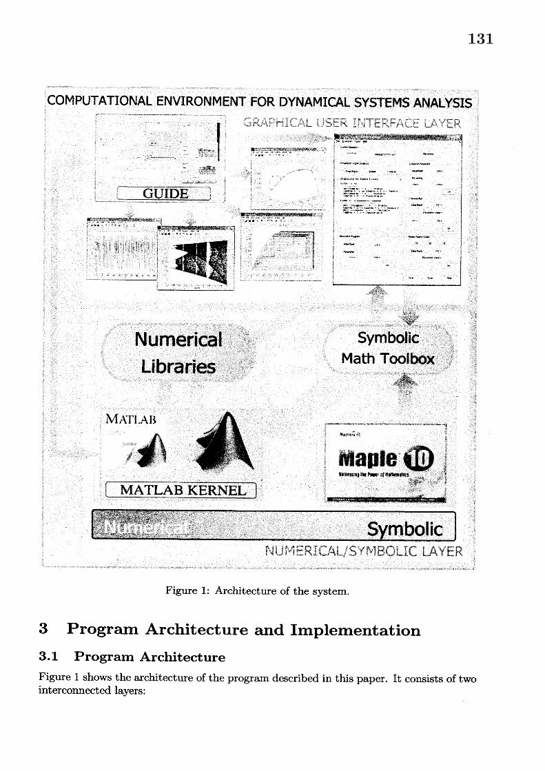
Figure 1: Architecture of the system.

3 Program Architecture and Implementation

3.1 Program ArchitectureFigure 1 shows the architecture of the program described in this paper. It consists of twointerconnected layers:

131

1. a $nume^{J}r^{v}ical$-symbolic layer it is basically a collection of numerical and symboliclibraries containing the commands, functions and routines implemented to performnumerical and symbolic tasks.

2. a graphical user interface $(GUI)$ layer. this component is responsible for input/outputwindowing, display of graphical output and smooth interaction with the user.

3.1.1 Numerical-symbolic layer

The nuinerical-symbolic layer is comprised of three different modules, according to thedistinct processes (numerical, symbolic and graphical) to be carried out:

1. a set of numericd librames containing the implementation of the commands, func-tions and routines for the numerical tasks. They have been implemented in thenative Matlab programming language. To this aim we take advantage of the largecollection of numerical routines available in the Matlab kernel such libraries are con-nected with. These standard Matlab routines provide extensive control on differentoptions and are fully optimized to offer the highest level of performance.

2. a set of symbolic routines and functions. They have been implemented by using theSymbolic Math Toolbox that provides access to several Maple routines for symbolictasks. This symbolic module is more important than it might seem at first sight;for instance, system equations are inputted symbolically so that some functionaloperators (such as derivatives) can be effectively applied. Further, some additionaloperators (string manipulation, forward/backward symbolic object-string conver-sion, symbol replacement and assigmnent, etc.) have also been used for symbolicpurposes. It is worthwhile to mention that the Symbolic Math Toolbox is less pow-erful than the Maple kemel system it comes from. Fortunately, it is also possibleto connect the kemels of Matlab and Maple for very specialized symbolic tasks.

3. some graphical commands. The powerful Matlab graphical capabilities exceed thosecomunonly available in other CAS such as Mathematica and Maple. Although ourcurrent needs do not require applying them at full extent, they avoid the users thetedious and time-consuming task to implement many routines for graphical outputby themselves. Some nice viewing features such as $3D$ rotation, zooming in andout, labeling, scaling, coloring and others are also automatically inherited from theMatlab graphical and windowing systems.

3.1.2 Graphical user interface layer

Although the libraries in previous layer are often enough to meet our computational needs,end-users might be challenged for using them properly unless they are really proficienton both Matlab syntax and functionalities and our implemented routines. This limita-tion can be overcome by creating a GUI; a well-designed GUI uses readily recognizablevisual cues to help the user navigate efficiently through information. Matlab provides apowerful mechanism to generate GUIs by using the so-called guide $(GUI$ DevelopmentEhvironment). This feature is not commonly available in many other CAS so far. Al-though its implementation requires - for complex interfaces - a high level of expertise,

132

it allows end-users to deal with our libraries with a minimal knowledge and input, thusfacilitating its efficient use and dissemination.

Based on this discussion, a GUI layer has been implemented. Some examples oftypical windows of our GUI are depicted in upper part of Figure 1. Some windows arefor user interaction-typicalIy input acquisition, parameter tuning and option selectiontasks. Others are windows to display graphical output. All them allow an effectiveuse of powerful interface tools designed according to the type of entities being displayed(e.g., drop-down menu for a choice list, check buttons for Boolean options, text boxesfor displaying messages, dialog boxes for input/output user interaction, etc.). Additionalfunctionalities are provided in hidden menus or in separate windows which can be invokedat will if needed so as to keep the main window streamlined and uncluttered. For instance,all graphical output is displayed in separate windows so that the information is betterorganized and flows in a natural and intuitive way. As a result, the system presents aGUI that is both aesthetic and very functional to the user.

3.2 Implementation issuesRegarding the implementation, thuis program has been developed by the author in Matlab$v2007b[17]$ running on Windows XP operating system by using a PC with Intel Core2 Duo processor at 2.4 GHz. and 2 GB of RAM. However, the program supports manydifferent platforms, such as PCs (with Windows $9x$ , 2000, NT, Me, XP and Vista) andUNIX workstations. A version for Apple Macintosh with Mac OS X system is alsoavailable provided that Mac Xll (the implementation of the X Window System thatmakes it possible to run Xll-based applications in Mac OS X) is properly installed andconfigured. Figures in this paper correspond to the PC platform version.

The graphical tasks are performed by using the Matlab GUI for the higher-level func-$tion\llcorner s$ (windowing, menus, or input) while the built-in graphics Matlab commands areapplied for rendering purposes. The numerical kernel has been implemented in the na-tive Matlab programming language, and the symbolic kernel has been created by usingthe commands of the Symbolic Math Toolbox.

4 Discrete SystemsThe program described in previous section is well suited for dealing with both discreteand continuous dynammical systems. This section illustrates the use of this software forthe case of discrete systems.

4.1 Fixed points and stabilityGiven an iterated map defined by a function $f(x)$ , a fixed point $x^{*}$ of $f(x)$ is a point thatis mapped to itself by the function, $i.e$ . $f(x^{*})=x^{*}$ . Let’s consider for example the logisticmap given by $x_{n+1}=\lambda x_{n}(1-x_{n})$ , where $n\in$ IN and $\lambda$ is a system parameter, usuallytaking values on the interval [0,4]. The logistic map became popular following a seminalpaper by the biologist Robert May in 1976 [18], where he introduced the discrete versionof a demographic model due to Verhulst. Roughly, $x_{n}\in[0,1]$ represents the populationat year $n$ , evolving from $x_{0}$ , the initial population value. Depending on the $\lambda$ value, the

133

a $arrow$

ffi $\zeta xmbs$ $Io*$ $M$

Systr Equim

$x(n\cdot 1)$ .$|mt,dQ^{\cdot}Y(n).t\uparrow Y(\cap))$

$Pu 6tcr$

Dynmcd $Sy\#-$ Andvsis $\llcorner Y\sim unov\in xp\alpha*$

$\Re..bllityotFlx\cdot dPo1mF|xedP\alpha|s.$

.$\theta*\iota_{V}$

. $|\overline{\underline{Co\mathfrak{m}pu!\epsilon}}|\wedge$$p_{Qn’\alpha r}lrdPr$

$x(0)\Rightarrow$

lxdPc $l1$ ) $\approx 0$ $\vee \mathfrak{n}$ . $\vee lh$ .$b\cdot(l\cdot\cdot bd\cdot)$ $\sim 1$ $–\triangleright$ St $b1$ .

$lmbd$. $-l$ $or$ $1\cdot*bd\cdot\cdot l$ $–\triangleright S\cdot ddl$. $\infty\alpha\backslash$

$b\cdot\prime l\cdot\cdot bd\cdot)$ $\triangleright\downarrow--\succ Un*t\cdot b1$ .$l\cdot\wedge bd\cdot\cdot$ $0$ $-\succ$ $S\backslash lp\cdot r*CUlo$

.. $c\alpha_{W}\alpha m$ $-$

$PxdPt(Z)$ $\cdot t1\cdot*bd\cdot-1)/1\cdot\cdot bd$ .$WP\alpha t$ $x(0)$ .

$b*(\tilde{-}*1\cdot\cdot bd*\}$ 4 1 $–>$ St $*b1$ .$1\cdot lbd$. . 1 or lmbda . 3 $–$ , Saddle I

$b\cdot t-Z+1\cdot*bd\cdot)$ $\succ 1--\geq un\mathfrak{s}C$ ab $l\circ$

$1\cdot-bd$. . $Z–\backslash$ Supa $r$ $*1$. $p\sim’\alpha ervdr$ .

$a\dagger^{-}uc\circ 0\alpha\vee-$

$rwPo t$ $x(0)$ .$p_{rdn\alpha*r}$

$vn$ . $\vee fh$ .$|\overline{\alpha \text{く}}|$

$xh$ . $x\prime \mathfrak{n}=$

$|\overline{(\supset\ltimes}|$

$\#rSp\kappa oCrW$

$\square 1D$ ロ 20 $\square 3D$

$i\urcorner 1-Po t$ $x(0)$ .$P\alpha’\alpha uw\iota r$ .

$\overline{\infty\alpha \text{く}}|$

$\overline{\infty c\infty}|||\overline{ckoe}||\overline{\}sr}|$

Figure 2: Fixed points and stability of the logistic map.

system evolves among a number of different situations, from the population eventuallydying to stabilizing or changing chaoticaly (see [18] for more details).

The program described in this paper can compute the fixed points of any iteratedmap. To do so, we must enter the system equation as shown in Figure 2. Note thatthe equation is given in a mathematical-looking way so that it can be subsequentlyprocessed for further symbolic-numerical calculations. For instance, we can also analyzethe stability of fixed points, by computing the eigenvalue of the fixed point, given by:

$\phi=[\frac{df(x)}{dx}]_{x=x^{*}}$ The fixed point is stable if $|\phi|<1$ , neutral if $|\phi|=1$ , unstable if

$|\phi|>1$ , and superstable if $|\phi|=0$ . The fixed points for the logistic map are: $x=0$ and$\lambda-1$

$x=\overline{\lambda}$. Figure 2 shows the fixed points of the logistic map along with their stability

analysis in terms of the $\lambda$ parameter.

4.2 Bifurcation diagramsDepending on the $\lambda$ value, the logistic map evolves among a number of different situa-tions. This behavior is better analyzed by using the bifurcation diagram, which shows

134

Figure 3: Bifurcation diagram of the logistic map on: (left) interval $[0,4]$ ; (right) interval[3.82, 3.86].

Figure 4: Bifurcation diagram of the cubic map on the interval [1, 4] for the initialconditions: (left) $x_{0}=0.5$ ; (right) $x_{0}=-0.5$ .

the possible long-term values (fixed points or periodic orbits) of a system as a functionof a system parameter. Figure 3 (left) shows the bifurcation diagram of the logistic mapfor $\lambda\in[0,4]$ . The initial input consists of the initial point $x_{0}$ and the initial and finalvalues of the system parameter. The bifurcation diagram is a fractal: if you zoom in onthe value $\lambda=3.825$ and focus on one branch of the diagram, the situation nearby lookslike a shrunk and slightly distorted version of the whole diagram, as shown in Figure 3(right). This is an example of the deep and ubiquitous connection between chaos andfractals.

An interesting scenario appears when the branches in the bifurcation diagram do

135

Figure 5: (left) Lyapunov exponent of the logistic map on the interval $[0,4]$ ; (right) closeup on the interval [3.2, 4].

depend on the initial values of the system variable, $x_{0}$ . This happens, for instance, forthe cubic map, given by: $x_{n+1}=(1-\mu)x_{n}+\mu x_{n}^{3}$ . This system has two fixed points of

the form $x_{1,2}=\pm\sqrt{\frac{\mu-1}{3\mu}}$ , meaning that there is no single value to display the whole

bifurcation diagram. Figure 4 displays the two bifurcation diagrams associated withthis map, obtained from two different initial conditions for the system variable, namely$x_{0}=0.5$ (left) and $x_{0}=-0.5$ (right). As the reader can see, there are two missingbranches of the period-4 orbits in each diagram, so both pictures are complementaryeach other.

4.3 Lyapunov exponentsOne indication of chaoticity is the so-called sensitivity to initial conditions, meaningthat two initially closed arbitrary trajectories diverge exponentially over the time. TheLyapunov exponent (LE) of a dynamical system is the number that characterizes therate of separation of these infinitesimaJly close trajectories along a given direction. Ofcourse, the rate of separation can be different for different orientations of initial separationvector, leading to as many Lyapunov exponents as the number of dimensions of the phasespace. LEs are intensively applied to analyze the behavior of nonlinear systems, sincethey indicate if small displacements of trajectories are along stable or unstable directions.In short, a negative LE is an indicator of regular (stable) behavior while a positive LEmeans that the orbit is unstable and chaotic.

Our program allows us to compute the Lyapunov exponents in a very easy way; theinitial input is given by the initial point for the system variable and the interval for thesystem parameter. Figure 5 (left) depictes the Lyapunov exponent of the logistic mapfor the system parameter on the interval $[0,4]$ . Comparison of this picture with Figure 3(left) shows that negative values for the LE are an indication of regular behavior, whilepositive values are associated with chaotic motion. Note also that the LE tends to-oo

136

Figure 6: Cobweb plot of the logistic map: (left) $\lambda=3.235;$ (right) $\lambda=4$ .

for $\lambda=2$ , meaning the existence of a superstable fixed point. Figure 5 (right) showsa magnification of the figure on the left for the interval [3.2, 4]. We can see that theLE is positive for $\lambda>3.569\ldots$ except by the existence of some periodic windows, thusexplaining very well the bifurcation diagram in Figure 3 (left).

4.4 Cobweb plotA cobweb plot is a graphical procedure especially suited to analyze the qualitative be-haviour of one-dimensional iterated fumctions. Cobweb plots are useful because they allowto determine the long-term evolution of an initial condition under repeated applicationof a map. Figure 6 shows two cobweb plots for the logistic map and the initial conditions$\lambda=3.235$ (left), and $\lambda=4$ (right). The first one shows the case of a period-2 orbit(represented by a rectangle) while the second case is a chaotic orbit.

4.5 Phase space graphA very powerful strategy to analyze chaotic systems is to use the so-called phase spacegraph By this we mean a collection of pictures associated with the orbit of a given point$x_{0}$ and embedded into different n-dimensional spaces. For $n=1$ we get the signal of theorbit, i.e. the sequence of iterates $\{x_{n}\}_{n}$ over the time. Such sequence is usually calledthe time serees. For $n=2$ the graph is obtained by representing the sequence of iterates$\{x_{n+1}\}$ vs. $\{x_{n}\}$ , for $n=3$, we represent the sequence of iterates $\{x_{n+2}\}$ vs. $\{x_{n+1}\}$ and$\{x_{n}\}$ and so on.

Figure 7 uses the phase space graph to analyze the chaotic behavior of the logisticmap for $\lambda=4$ . These pictures illustrate perfectly how the chaotic behavior looks like. Onthe left, the signal of the orbit is displayed. As discussed above, a characteristic of chaosis that chaotic systems exhibit a great sensitivity to initial conditions. A common sourceof such sensitivity to initial conditions is that the map represents a repeated folding andstretching of the space on which it is defined. The $n=2$ phase space graph for the

137

Figure 7: (left to right) lD, $2D$ and $3D$ phase space graph for the logistic map.

logistic map, represented in Fig. 7 (middle), gives a two-dimensional phase diagram ofthe logistic map showing the quadratic curve of its iterated equation. We can also embedthe same sequence in a $3D$ phase space, in order to investigate a deeper structure of themap. Figure 7 (right) shows how initially nearby points begin to diverge, particularly inthose regions corresponding to the steeper sections of the plot.

5 Continuous SystemsIn this section we show some applications of the program through illustrative examplesfor the case of continuous systems. In thuis work we restrict ourselves to the case of finite-dimensional flows, whuich are mathematically described by systems of ordinary differentialequations.

5.1 Symbolic-numerical analysis

Figures 8-11 show screenshots of a typical session for analyzing $3D$ continuous systems.The session workflow is as follows: firstly, the user inputs the system equations expressedsymbolically. For instance, in Figure 8 we consider the famous Lorenz system [16], givenby: $(x’, y’, z’)=(\sigma(y-x), (R-z)x-y, xy- bz)$ where $\sigma,$ $R$ and $b$ are the systemparameters. The program includes a module for the computation of the Jacobian matrixand the equilibrium points of any finite-dimensional flow. The Jacobian matrix is asquare matrix whose entries are the partial derivatives of the system equations withrespect to the system variables. If no value for the system parameters is provided, thecomputation is performed symbolically and the corresponding output depends on thosesystem parameters. The equilibrium points and the eigenvalues and eigenvectors of thesystem can also be computed in a similar way.

Figure 8 shows the symbolic Jacobian matrix for the Lorenz system, which dependsnot only on the system parameters but also on the system variables. Once some parametervalues are given ($\sigma=10,$ $R=60$ and $b=8/3$ in this example), the Lyapunov exponents(LE) of the system can be numerically computed. To this purpose, a numerical integrationmethod is applied [20]. The corresponding options and parameter values are shown inFigure 9. The numerical values of these LE are 1.4, 0.0012 and-15 respectively. Theirgraphical representation over the time is depicted in Figure 10.

138

Figure 8: Symbolic Jacobian matrix for the Lorenz system.

Roughly speaking, LEs are a generalization of the eigenvalues for nonlinear flows. Inparticular, a negative LE indicates that the trajectory evolves along the stable directionfor this variable (and hence, regular behavior for that variable is obtained) while a positivevalue indicates a chaotic behavior.

5.2 Visualization of chaotic attractorsSince in our example we find positive LE, the system exhibits a chaotic behavior. Thisfact is evidenced in Figure 11 (left) where the corresponding attractor and the equilibriumpoints of the Lorenz system for our choice of the system parameters are displayed. Theircorresponding numerical values are shown in the main window of Figure 9. Finally, Figure11 (right) shows the evolution of the system variables over the time from $t=0$ to $t=50$ .

In order to display the attractor and/or the evolution of the system variables over thetime (like in Figure 11), some kind of numerical integration is required. The program inthis paper allows end-users to choose different numerical integration methods [20], includ-ing the classical Euler and 2nd- and $4th$-order Runge-Kutta methods (implemented bythe author) along with some more sophisticated methods from the Matlab kemel such asode45, ode23, ode113, ode $15s$ , ode$23s$ , ode$23t$ and ode$23tb$ (see [17] for details). Someinput required for the numerical integration (such as the initial point and the integrationtime) is also given at this stage. By pressing the “Numerical Integration settings” button,some additional options (such as the absolute and relative error tolerance, the initial and

139

Ek $E\cross wvusI’*$ $M$

Systm $E\eta udW$.-.

$x$ . $\Psi^{\mathfrak{n}obx|}$

$\mu$ $R.\nu*x.$ .:. $xyb^{\backslash }$

$-\sim-7_{\}$

System wrdr$s$

$1rA9dlrTm$

$ur$. $0$ $M\sim$ 50

$|n_{C}9dr$ Nethod

ode45 $su|r9$ $|$

$h\star$ . An $u\cdot\cdot\n$ one wndos

$y^{1}$. $Sr*$ am $Se$veiel axes

$p|$$\mathbb{E}aeh1\cdot e\mathfrak{n}$ one $1W1\omega$

OK $|$

Cm $|$ $cb,$. $|$ $H*$ $|$

Figure 9: Equilibrium points and Lyapunov exponents for the Lorenz system.

Figure 10: Temporal evolution of the Lyapunov exponents for the Lorenz system.

maximum stepsize and refinement, the computation speed and others) can be set up in aseparate window. Then the user proceeds with the graphical representation stage, wherehe$/she$ can display the attractor of the dynamical system and/or the evolution of any ofthe system variables over the time. Such variables can be depicted on the same or ondifferent axes and windows. The“Graphical Representation settings” button opens a newwindow where different graphical options such as the line width and style, markers for theequilibrium points, and some coloring options can be defined. The result is the graphical

140

Figure $\ovalbox{\tt\small REJECT}\ovalbox{\tt\small REJECT}\cdot r_{O^{r}C17}lrs)^{r}SCem$. $(|_{t^{J}}fC)c\dagger\iota$ aot $1C_{Cv}^{\neg}fCractol$ . and equilibrium points; (right) tempo-ral $evolutt_{O^{n}}o^{f}s\gamma sCc\tau r\iota var\iota$ ablcs.

Figure 12: Chaotic attractors of $3D$ flows: (top-left) Lorenz system; (top-right) R\"osslersystem; (bottom-left) Van-der-Pol Duffing oscillator; (bottom-right) Chua’s circuit.

141

output shown in Figure 11 where the chaotic attractor and the temporal evolution of thesystem variables are displayed.

Figure 12 shows the chaotic attractors of four distinct nonlinear flows: Lorenz systemfor weather forecasting, R\"ossler chemical reaction, Van-der-Pol Duffing oscillator andChua’s electronic circuit (see [19] for further information about these systems).

AcknowledgmentsThe author would like to express her sincere acknowledgment and appreciation to Prof.Setsuo Takato for his kind invitation to participate in this RIMS workshop and visit thelovely city of Kyoto, and for creating such a friendly atmosphere during all my stay inJapan. I really hope we can meet again very soon.

This research has been supported by the Computer Science National Program ofthe Spanish Ministry of Education and Science, Project Ref. #TIN2006-13615 and theUniversity of Cantabria.

References[1] The Bologna Declaration on the European space for higher education: an explanation.

Association of European Universities&EU Rectors’ Conference (1999) pp. 4 (availableat: $http.\cdot//ec.europa.eu/education/policies/educ/bologna/bologna.pdf)$ .

[2] Chua, L.O., Komuro, M., Matsumoto, T.: The double-scroll family. IEEE $\mathcal{I}hnsac-$

tions on Circuits and Systems, 33, (1986) 1073-1118.

[3] Dhooge, A., Govaerts, W., Kuznetsov, Y.A.: Matcont: A Matlab package for nu-merical bifurcation analysis of ODEs. ACM Transactions on Mathematical Software,29(2) (2003) 141-164

[4] Dhooge, A., Govaerts, W., Kuznetsov, Y.A.: Numerical continuation of fold bifurca-tions of limit cycles in MATCONT. Lecture Notes in Computer Science, 2657 (2003)701-710

[5] G\’alvez, A.: Numerical-symbolic Matlab program for the analysis of three-dimensionalchaotic systems. Lectures Notes in Computer Science, 4488 (2007) 211-218

[6] G\’aJvez, A.: Matlab toolbox and GUI for analyzing one-dimensional chaotic maps.Intemational Conference on Computational Science and Applications, ICCSA2008,IEEE Computer Society Press, Los Alamitos, CA, (2008) 211-218.

[7] G\’aJvez, A., Iglesias, A.: Symbolic/numeric analysis of chaotic synchronization with aCAS. Future Genemtion Computer Systems 25(5) (2007) 727-733

[8] Govaerts, W., Sautois, B.: Phase response curves, delays and synchronization inMatlab. Lectures Notes in Computer Science, 3992 (2006) 391-398

[9] Guti\’errez, J.M., Iglesias, A., Gu\’emez, J., Mat\’ias, M.A.: Suppression of chaos throughchanges in the system variables through Poincar\’e and Lorenz return maps. Intema-tional Joumal of Bifurcation and Chaos, 6 (1996) 1351-1362

142

[10] Guti\’errez, J.M., Iglesias, A.: A Mathematica package for the analysis and control ofchaos in nonlinear systems. Computers in Physics, 12(6) (1998) 608-619

[11] Iglesias, A.: A new scheme based on semiconductor lasers with phase-conjugatefeedback for cryptographic communications. Lectures Notes in Computer Science,2510 (2002) 135-144

[12] Iglesias, A., G\’alvez, A.: Analyzing the synchronization of chaotic dynamical systemswith Mathematica: Part I. Lectures Notes in Computer Science, 3482 (2005) 472-481

[13] Iglesias, A., Ga’lvez, A.: Analyzing the synchronization of chaotic dynamical systemswith Mathematica: Part II. Lectures Notes in Computer Science, 3482 (2005) 482-491

[14] Iglesias, A., G\’alvez, A.: Revisiting some control schemes for chaotic synchronizationwith Mathematica. Lectures Notes in Computer Science, 3516 (2005) 651-658

[15] Lauwerier, H.A.: One-dimensional iterative maps. In: Chaos. Holden, A.V. (ed.).Manchester University Press, Manchester (1986)

[16] Lorenz, E.N., Deterministic nonperiodic flow, Joumal of Atmospheric Sciences, 20(1963) 130-141.

[17] The Mathworks Inc: Using Matlab. Natick, MA (1999)

[18] May, R.M.: Simple mathematical models with very complicated dynamics. Nature261 (1976) 459-467

[19] Ott, E.: Chaos in Dynamical Systems. Cambridge University Press, Cambridge(1993)

[20] Press, W.H., Teukolsky, S.A., Vetterling, W.T., Flannery, B.P.: Numerical Recipes(2nd edition), Cambridge University Press, Cambridge, 1992.

[21] Sarafian, H.: A closed form solution of the run-time of a sliding bead along a freelyhanging slinky. Lecture Notes in Computer Science, 3039 (2004) 319-326

[22] Zhou, W., Jeffrey, D.J. Reid, G.J.: An algebraic method for analyzing open-loopdynamic systems. Lecture Notes in Computer Science, 3516 (2005) $586rightarrow 593$

143