Physics 221: University Physics Laboratory

Laboratory Manual

Montana State University-Billings

Lab # 1 Specific Heat and Calorimetry

Theory: The specific heat (c) of an object is defined by the equation that relates the heat energy (Q) absorbed by an object of mass m to its corresponding increase in temperature (∆T): Q = mc∆T. If two different objects with different temperatures are brought into contact and isolated from the rest of the world, they exchange thermal energy until they reach a common equilibrium temperature. Mathematically, this can be written as Qlost = Qgained or

m 1c1 T1 − Te( )= m 2c2 Te − T2( ) (1) where m1 and m2 are the masses of objects 1 and 2, respectively, and object 1is initially warmer than object 2. This statement is nothing more than conservation of energy applied to the notion of heat energy. We can exploit this property to find the specific heat of one substance in terms of the known specific heat of another. Since the specific heat of water is defined to be

1 cal

g ⋅°C , we can therefore measure the specific heat of any object

by heating it up and immersing it in a bath of cool water. The specific heat of the object (1) is then related to the specific heat of water (object 2) by:

c1 = c2

m 2 Te − T2( )m 1 T1 − Te( )

. (2)

Therefore, to measure c1 we need to measure m 1 , m 2 , T1 , T2 , and Te . We will follow this general procedure in this lab to measure the specific heat of an unknown substance and identify the substance by comparing the specific heat to a table of specific heats. A word of caution is appropriate here. We will use mercury-filled thermometers to measure temperatures. Mercury is a toxic heavy metal. Please be careful not to break the thermometers! Procedure: The device used to isolate the water and the unknown object from the rest of the universe is known as a calorimeter. Our calorimeters are constructed of aluminum and consist of two cans -- an inner can (which holds the water) and an outer can which keeps the universe at bay. Unfortunately, the inner can becomes part of the system and so it also absorbs heat from the unknown object. If the inner aluminum can and the water have the same initial temperature T2, equation (2) becomes with the inclusion of the unknown object

( ) ( )

( )e

eAlAlewaterwater

TTmTTcmTTcm

c−

−+−=

11

221 . (3)

where c1, m1, and T1 are the specific heat, mass, and initial temperature, respectively, of the unknown object, and Te is the final or equilibrium temperature of the system (the water, aluminum inner can, and unknown object). The first thing we must do is measure the specific heat of the inner can or cAl. Once this is known, we can solve equation (3) for the specific heat of the unknown object. First, measure the mass of the empty inner can. This is mass m1 in Eq. 2. mAl = m1 __________ . Now immerse the inner can in the ice water bath provided and let it cool for a few minutes until it reaches the temperature of the ice water. Record this temperature with your thermometer. This is temperature T1 in Eq. 2. Tice water = TAl = T1 = ___________. Pour about 100 ml of room temperature water into a beaker. Measure and record the temperature of this water. This is temperature T2 in Eq. 2. Twater = T2 = _____________.

Quickly remove the inner can from the ice water, dry off any excess water, pour the room temperature water from the beaker into the inner can, reassemble the calorimeter, and insert the thermometer into the calorimeter.. Again, this must be done quickly. Let the calorimeter come to an equilibrium temperature. This will take a few minutes. Record this temperature. Te = ___________. Remove the inner can without spilling any water and find the mass of this full can. The mass of the water in the can is the mass of the full can minus the mass of the empty can. This is mass mre2 in Eq. 2. Record these values. mwater = mfull – mempty = m2 = _________________________________________. Use this data to find cAl = c1 using equation (2). Show your calculations. In Eq. 2 c2 = cwater cAl = c1 =______________. Next, place the inner can full of water back into the calorimeter. Find and record the mass of the unknown sample. Refer to Eq. 3 for this part of the lab. m1 = ___________________. Tie the unknown substance to a string and hang it in the boiling water provided. Record the temperature of the boiling water (DO NOT USE THE THERMOMETER FROM

THE CALORIMETER). This is also the temperature T1 of the unknown. Record this value.

T1 = ____________. Record the temperature T2 of the water in the calorimeter (DO NOT USE THE THERMOMETER FROM THE BOILING WATER). This is also the temperature of the inner can.

T2 = ______________. Quickly remove the unknown sample from the boiling water and place it into the calorimeter. Allow the water and the unknown object to reach an equilibrium temperature. Record this temperature.

Te =_______________. Using equation (3), calculate the specific heat of the unknown substance. Show your work.

c1 = ____________. Identify the unknown substance.

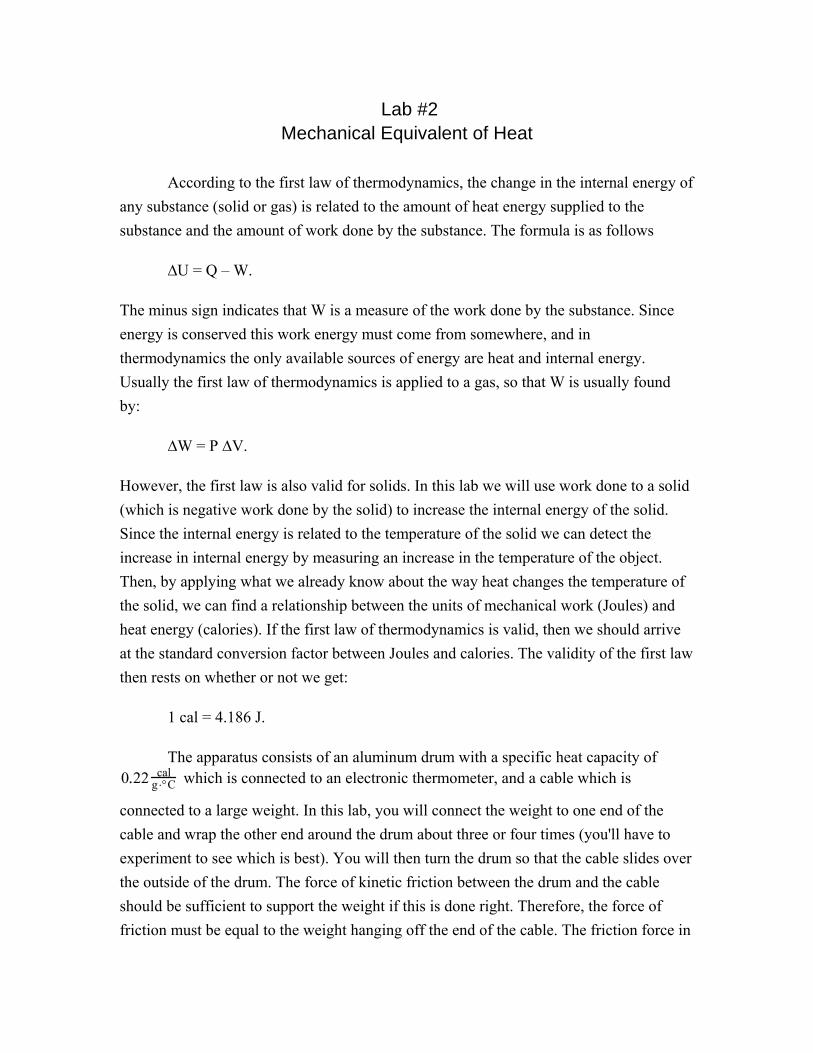
Lab #2 Mechanical Equivalent of Heat

According to the first law of thermodynamics, the change in the internal energy of any substance (solid or gas) is related to the amount of heat energy supplied to the substance and the amount of work done by the substance. The formula is as follows

∆U = Q – W.

The minus sign indicates that W is a measure of the work done by the substance. Since energy is conserved this work energy must come from somewhere, and in thermodynamics the only available sources of energy are heat and internal energy. Usually the first law of thermodynamics is applied to a gas, so that W is usually found by:

∆W = P ∆V.

However, the first law is also valid for solids. In this lab we will use work done to a solid (which is negative work done by the solid) to increase the internal energy of the solid. Since the internal energy is related to the temperature of the solid we can detect the increase in internal energy by measuring an increase in the temperature of the object. Then, by applying what we already know about the way heat changes the temperature of the solid, we can find a relationship between the units of mechanical work (Joules) and heat energy (calories). If the first law of thermodynamics is valid, then we should arrive at the standard conversion factor between Joules and calories. The validity of the first law then rests on whether or not we get:

1 cal = 4.186 J.

The apparatus consists of an aluminum drum with a specific heat capacity of

0.22 cal

g ⋅°C which is connected to an electronic thermometer, and a cable which is

connected to a large weight. In this lab, you will connect the weight to one end of the cable and wrap the other end around the drum about three or four times (you'll have to experiment to see which is best). You will then turn the drum so that the cable slides over the outside of the drum. The force of kinetic friction between the drum and the cable should be sufficient to support the weight if this is done right. Therefore, the force of friction must be equal to the weight hanging off the end of the cable. The friction force in

the cable is tangent to the surface of the drum and is sliding over the drum, the work done by the cable on the drum is equal to the force of friction times the distance that the cable travels over the edge of the drum. The value of this work is:

W = Ff × d = mg( )× 2πrn( )

where n is the number of revolutions of the drum. The work done by the drum is simply the negative of this value. There is no heat supplied to the drum so all of this work goes into increasing the internal energy of the drum. Therefore,

∆U = 2πrmg × (number of turns).

The units of this are Joules if m is measured in kilograms and g is measured in m s 2 .

The internal energy could also have been changed this amount by adding heat and doing no work. This would result in a change in temperature found by:

∆U = Q = Mc∆T,

where M is the mass of the drum and c is the specific heat of aluminum. The units of ∆U in this calculation are calories if M is measured in grams and c is taken to be 0.22. By measuring ∆T, and M, we can find ∆U in calories and compare it to the ∆U found in Joules. Thus,

McΔT2πrmgn

=1

4.186calJ

.

Procedure:

Unscrew the black knob and remove the aluminum drum. Place the drum in ice to bring the temperature down to at least 10°C below room temperature. While the drum is cooling, plan the desired temperature variation of the experiment. Ideally, the temperature variation of the drum should be from 7-9°C below room temperature to the same amount above room temperature. Therefore, measure the room temperature and then determine and record the initial and final temperatures you wish to use for the drum.

Ti = Tf =

Use the table of Resistance vs. Temperature which is on the apparatus to determine the resistances which correspond to these temperatures and record these values:

Ri = Rf =

When the drum is sufficiently cool, dry it off and slide it back on the crank shaft. Be sure that the copper plated board is facing toward the crank. Replace the black knob and tighten it. Wrap the cable several times around the drum, making surre that the cable lies flat against the drum. Set the counter to zero. Watch the ohmmeter carefully and begin cranking when the resistance is equal to Ri . Crank rapidly until the resistance approaches

Rf . At this point start cranking more slowly. When the resistance is Rf , stop cranking

and watch the ohmmeter. When the resistance reaches a minimum and starts to go back up, record the minimum value as Rm . Use the table to determine the corresponding temperature, Tm .

Rm = Tm =

Record the number of turns given on the counter:

n =

Measure the diameter of the drum with calipers and record it

2r =

Find the masses of the weight and the drum and record these as m and M

m = M =

Calculate the ratio

McΔT2πrmgn

using ΔT = Tm − Ti

Find the percent difference between this value and

14.186

Lab #3 Electrostatic Experiments

Introduction: According to modern atomic theory, matter is made up of small, indivisible chunks. Electricity also appears to come in small indestructible, indivisible pieces. This is by no means obvious at all. The model we have come to accept is based on hundreds of years of experimentation and observation. It is fairly easy to visualize and accounts for many observations as you will see. Electric charge comes in two kinds. If you rub the hard rubber rod with cat's fur, electrons are removed from the fur and get wiped onto the rod. This gives the rod a slight, excess negative charge. If you touch the top of your electroscope with the rod some of the electrons move over onto the electroscope. Do this at watch the leaves diverge. The two negatively charged leaves repel each other and therefore move apart. Charge the rubber rod again and move it close to the top of the electroscope but do not touch it to the knob. What you see could be caused by electrons moving away from the knob of the electroscope and going down to the leaves. It turns out that the negatively charged electrons are free to move in the metal parts of the electroscope and the positive charges do not move. Notice, however, that you couldn't determine that from any of these experiments. Now go ahead and actually charge the electroscope by touching the knob with the rod. While the electroscope is still negatively charged, rub the glass rod with the piece of silk cloth which you will find at your station. This causes electrons to be wiped from the glass rod which then leaves a net positive charge. Bring the glass rod close (not too close) to the knob. What do you see? Explain what this means in terms of the electrons in the electroscope. Explain how this demonstrates that there are two kinds of charge.

Touch the knob with your finger to ground the electroscope. Charge up the rubber rod and hold it close enough to the ball that the leaves spread a bit. Some of the electrons in the electroscope are pushed down into the leaves in order to get away from the negatively charged rod. Without moving the rod away, touch the knob with the finger of your other hand. Take your finger away without moving the rod. The leaves should now be hanging down. Now, move the rod away. The leaves should spread back apart. This means that the electroscope is now charged. Determine the sign of the charge of the electroscope and record your answer: Explain in terms of moving electrons how you managed to charge the electroscope. Hang the aluminum cup from a glass rod, charge up the rubber rod with the cat's fur and touch the aluminum cup with the rubber rod in order to charge it. Now take a proof plane (the little aluminum lollipop-like gizmo) and carefully reach down inside the cup and touch the bottom of the cup with the proof plane. Remove the proof plane without touching the sides of the cup and touch the knob on the electroscope with it. If there is any charge on the proof plane, the leaves of the electroscope should diverge. Do they? Now repeat this but touch the outside of the cup instead of the inside. Do the leaves diverge? This should show that all of the charge resides on the outside of a conducting body. Explain in terms of moving charges why this should be true.

Lab # 4 Ohm's Law

One of the more important principles in current electricity is known as Ohm's Law. This law, or some modification of it, is used whenever it is necessary to calculate the current flowing in an electrical circuit. Electric charge moving through a conductor (such as a wire) is called an electric current flow. The current is defined to be the amount of charge that passes by any point in the circuit in one second. A potential difference, or voltage is necessary to establish a current. It is found that the potential difference existing between the two ends of most conductors is directly proportional to the current flowing through the conductor. Any conductor for which this is true is said to obey Ohm's law. It is the object of this experiment to study Ohm's law and the laws relating to series or parallel circuits. It is useful in the study of electrical circuits to keep in mind the fluid flow models developed previously. The electrical current (coulomb's per second or amperes) is analogous to a water flow in gallons/sec. The voltage or potential difference is like a pressure or pressure drop. A high resistance conductor corresponds to a narrow pipe and hence little flow and lots of pressure drop, or little current and large voltage. The ammeter is essentially like a flow rate meter and the voltmeter is like a pressure meter. A battery or power supply is like a pump which keeps everything moving. Theory: Ohm's law states that the numerical value of the current in a conductor is equal to the total potential drop, or voltage, across the conductor divided by the resistance of the conductor. Mathematically:

I =

VR

or V = IR

where V is the voltage across the conductor in volts, R is the resistance (measured in Ohms -- Ω), and I is the current in amperes. The numerical value of the resistance of a given conductor depends on a number of factors (e.g.: material, length, diameter, etc.). When resistances are connected in series, the current is the same at all points throughout the circuit. The sum of the voltage drops across the individual resistances is equal to the total applied voltage and the total resistance of the circuit is equal to the sum of the individual resistances.

When resistances are connected in parallel, the voltage drop is the same across all the resistances. The sum of the currents across each resistor is equal to the total current generated by the battery or power supply and the total resistance of the circuit is found by:

1Rtotal

=1

Rnn∑

Procedure: Connect the power supply, ammeter, voltmeter and resistors as shown:

Measure the current and the voltage given by the meters: I = V = Using Ohm's Law, calculate the effective resistance of the circuit: R = Now connect the voltmeter across each resistor individually and measure the voltage drops across each resistor: V1 =

V2 =

Knowing that the current is the same through each resistor, calculate the resistance of each resistor using Ohm's Law: R1 =

R2 =

Calculate the effective resistance using these values and the formula given: Rtotal = R1 + R2 =

How does this compare with the value of R measured above? Next, construct the circuit shown:

Measure the currents through each ammeter:

I1 =

I2 =

I =

and the voltage across the voltmeter:

V = Use Ohm's law to find the effective resistance and the individual resistances of this parallel circuit:

R1 =

R2 =

R =

Use the formula given above to calculate the effective resistance using the values of R1 and R2 which you have measured.

Rtotal =

How does this compare with the measured effective resistance?

Lab # 5 Kirchhoff's Rules

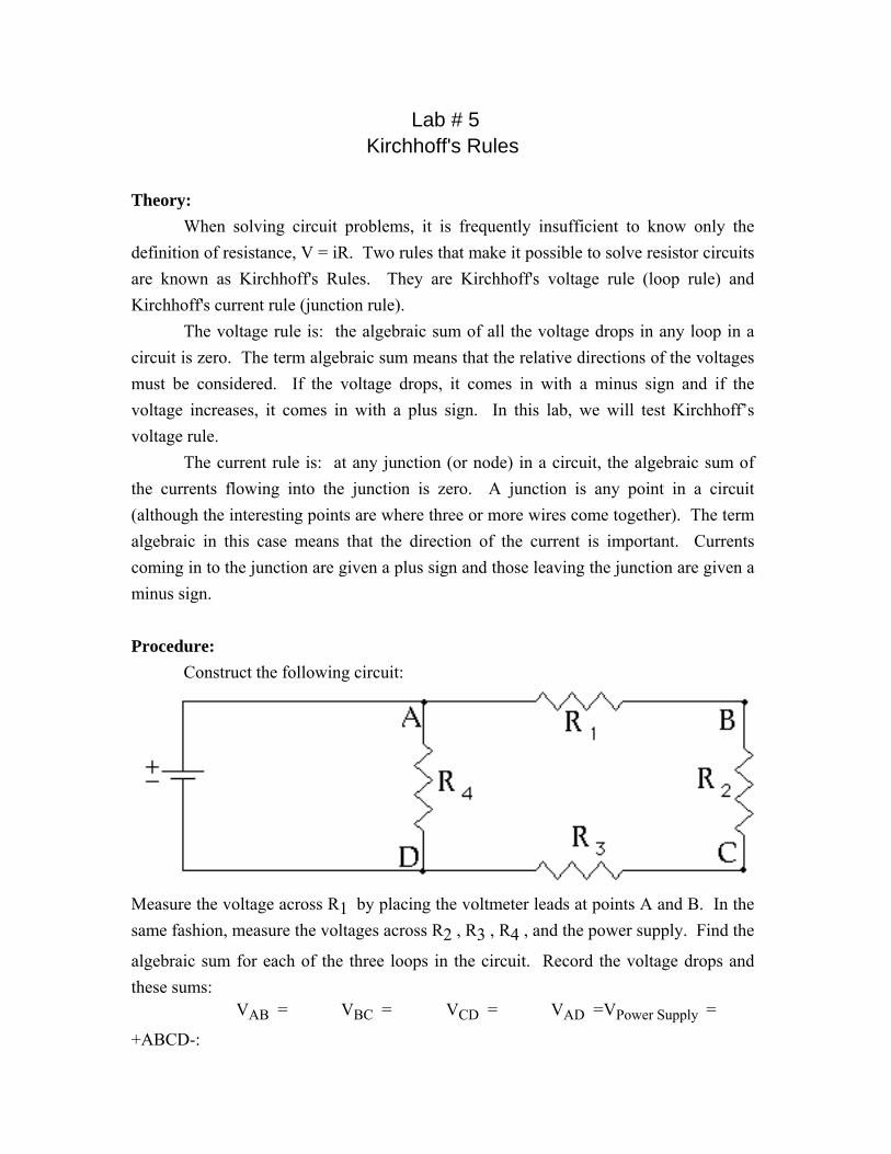
Theory: When solving circuit problems, it is frequently insufficient to know only the definition of resistance, V = iR. Two rules that make it possible to solve resistor circuits are known as Kirchhoff's Rules. They are Kirchhoff's voltage rule (loop rule) and Kirchhoff's current rule (junction rule). The voltage rule is: the algebraic sum of all the voltage drops in any loop in a circuit is zero. The term algebraic sum means that the relative directions of the voltages must be considered. If the voltage drops, it comes in with a minus sign and if the voltage increases, it comes in with a plus sign. In this lab, we will test Kirchhoff’s voltage rule. The current rule is: at any junction (or node) in a circuit, the algebraic sum of the currents flowing into the junction is zero. A junction is any point in a circuit (although the interesting points are where three or more wires come together). The term algebraic in this case means that the direction of the current is important. Currents coming in to the junction are given a plus sign and those leaving the junction are given a minus sign. Procedure: Construct the following circuit:

Measure the voltage across R1 by placing the voltmeter leads at points A and B. In the same fashion, measure the voltages across R2 , R3 , R4 , and the power supply. Find the

algebraic sum for each of the three loops in the circuit. Record the voltage drops and these sums: VAB = VBC = VCD = VAD = VPower Supply =

+ABCD-:

ABCD: +AD-: Are these numbers sufficiently small compared to the individual voltage drops to be within experimental error of zero? Next, place the negative meter lead at point D. Measure the voltage drop across R1 via the following procedure: Place the positive meter lead at A and record VAD , then place the positive meter lead at B and record VBD . The voltage across R1 is given by the difference VAD − VBD . Repeat this procedure to measure the voltage across the

other resistors and record these values. VAB = VAD − VBD = VBC = VBD − VCD = VCD = VAD =

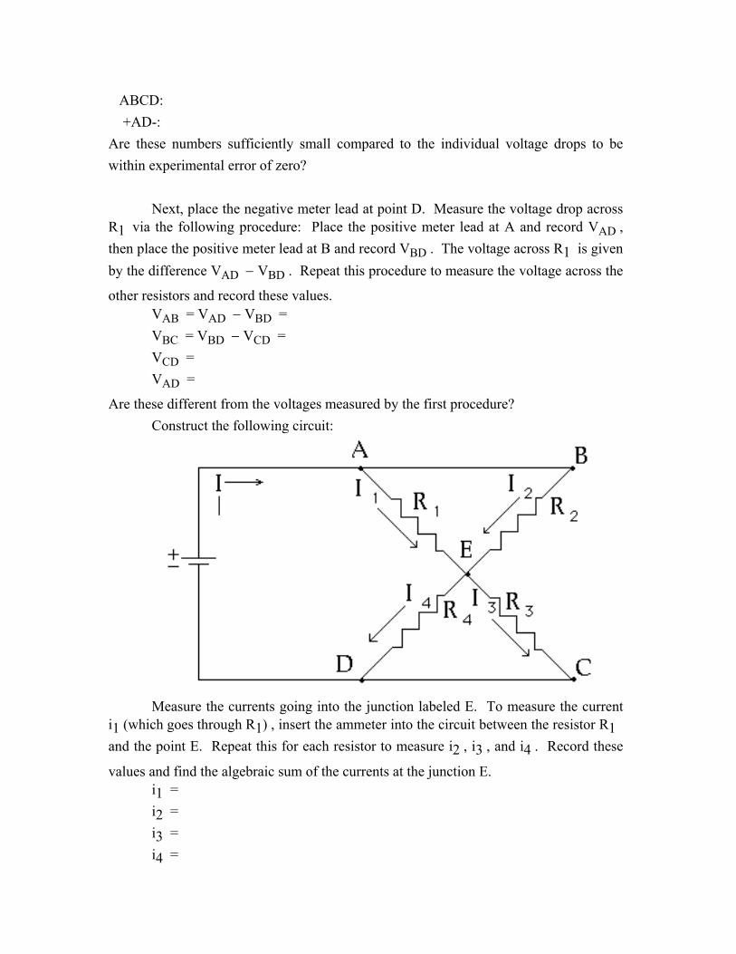
Are these different from the voltages measured by the first procedure? Construct the following circuit:

Measure the currents going into the junction labeled E. To measure the current i1 (which goes through R1) , insert the ammeter into the circuit between the resistor R1 and the point E. Repeat this for each resistor to measure i2 , i3 , and i4 . Record these

values and find the algebraic sum of the currents at the junction E. i1 = i2 = i3 = i4 =

∑n=1

4 in =

Is the sum within experimental error of zero? From the measured values of i1 , i2 , i3 , and i4 , find the current (I) coming out

of the power supply. Measure the voltage across the power supply and find the effective resistance of the circuit by:

Reff = VI =

Using the known values of R1 , R2 , R3 , and R4 , calculate Reff : Reff =

Is the calculated value within experimental error of the measured value?

Lab # 6 Faraday's Law of Induction

Theory: Faraday's law of induction states that a changing magnetic flux generates an electric field which can be described by:

EΔlcosθloop∑ =

−Δ BΔA cosϕarea∑

⎛

⎝ ⎜ ⎞

⎠ ⎟

Δt.

If the magnetic field is fairly uniform in direction, then the lines of the induced electric field are circular. A loop of wire placed in this circular electric field will carry current that is driven by the electric field. This current is given by:

I =

VR

= −NR

ΔΦB

Δt

where N is the number of turns in the loop of wire, R is the resistance of the wire, and ΦB is the flux passing through the loop. The minus sign is a statement of Lenz's Law

that is simply conservation of energy applied to this system. In this lab, we will explore the consequences of Faraday's Law. Procedure: Two coils of wire have been supplied which fit one inside the other. The larger coil is to be connected to a DC power supply so that it acts as a magnet. The magnetic field created by the coil resides primarily inside the coil. If the other coil is connected to a galvanometer (a sensitive but uncalibrated ammeter) and inserted into the larger coil, then the magnetic flux through the small coil changes from zero to what ever value the flux is inside the larger coil. This changing flux will generate a current in the small coil. Note that if the small coil is slowly pushed into the large coil then the rate of change of flux is small and so the current is small and if the rate of change is large, the current will be large. Record the size and direction of the deflection of the needle on the galvanometer (e.g.: small, to the right) for the following cases:

deflection size direction

large current, fast large current, slow small current, fast

small current, slow Some substances behave like the magnetic equivalent of a dielectric and are called ferromagnets. These substances have intrinsic magnetic dipoles that tend to align themselves with any ambient magnetic field, thereby enhancing the field inside the substance. Iron is a typical ferromagnet. To see the effect that iron has on the magnetic field inside a coil, place the small coil inside the large coil and then insert the iron rod into the small coil. What is the deflection on the galvanometer? Record the direction and size of the deflection when the iron rod is inserted and when it is removed.

deflection size direction

insert remove

Look at the direction that the wires are wrapped in the small coil. Does the direction of the current correspond to Lenz's Law?

Lab # 7 R-C Circuits

A circuit consisting of a resistor in series with a capacitor will have a time varying current that produces a time varying voltage drop across both the capacitor and the resistor. Initially, the voltage drop across the capacitor is zero and the voltage drop across the resistor is equal to the EMF supplied to the circuit. After a long period of time, the voltage drop across the capacitor will grow until it is equal to the EMF and the voltage drop across the resistor shrinks to zero. The exact time dependence of the voltage drop across the capacitor is given by: Vcap = E 1− e −t RC( ) where E is EMF in volts. This expression gives meaning to the phrase "long period of time" used above. When t » RC, then the exponent goes to zero, and so the voltage across the capacitor reaches its maximum — E. The value RC is called the time constant of the R-C circuit since it defines a natural time scale to be used. When t = RC, the voltage across the capacitor has reached 63% of E. We will use this fact to experimentally check the time constant for an R-C circuit. In addition you will get some experience using an oscilloscope. Procedure: Construct the following circuit on breadboard, and connect the leads to the oscilloscope as shown:

The EMF will be supplied to the circuit in the form of a square-wave alternating current. This has the effect of connecting a battery to the circuit and switching the poles at regular

intervals. The rate of switching is equal to the frequency of the square-wave. The oscilloscope will show the voltage across the capacitor as it charges up to +E and charges down to -E (note: it does not discharge!). The curve on the oscilloscope will look like:

The grid on the oscilloscope provides scale markings so that the horizontal axis reads time and the vertical axis reads voltage. The numerical values of the scale can be read off of the dials. Adjust both the amplitude of the square wave and the scale on the vertical axis so that the voltage drop across the capacitor covers 5 divisions. Find the point at which the voltage grows from zero to 3.2 (64% of maximum) on the vertical axis. The horizontal axis will tell you the time required for this growth (which is the time constant). Record this value: t = The time constant can be calculated from the known values of the resistor and capacitor. Find these values and calculate the time constant: R = C = t = RC = Is your measured t equal to RC? (Within experimental error)

Lab # 8 L-C Circuits

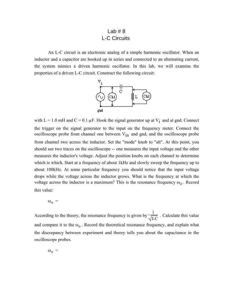
An L-C circuit is an electronic analog of a simple harmonic oscillator. When an inductor and a capacitor are hooked up in series and connected to an alternating current, the system mimics a driven harmonic oscillator. In this lab, we will examine the properties of a driven L-C circuit. Construct the following circuit:

with L = 1.0 mH and C = 0.1 μF. Hook the signal generator up at Vi and at gnd. Connect

the trigger on the signal generator to the input on the frequency meter. Connect the oscilloscope probe from channel one between Vin and gnd, and the oscilloscope probe

from channel two across the inductor. Set the "mode" knob to "alt". At this point, you should see two traces on the oscilloscope -- one measures the input voltage and the other measures the inductor's voltage. Adjust the position knobs on each channel to determine which is which. Start at a frequency of about 1kHz and slowly sweep the frequency up to about 100kHz. At some particular frequency you should notice that the input voltage drops while the voltage across the inductor grows. What is the frequency at which the voltage across the inductor is a maximum? This is the resonance frequency ωo . Record

this value: ωo =

According to the theory, the resonance frequency is given by 1LC

. Calculate this value

and compare it to the ωo . Record the theoretical resonance frequency, and explain what

the discrepancy between experiment and theory tells you about the capacitance in the oscilloscope probes. ωo =

Set the signal generator at the resonance frequency and sketch the traces on the oscilloscope. Repeat this for frequencies that are well below and well above the resonance frequency. Be sure to draw exactly what you see on the oscilloscope -- especially the relative phases of the traces.

Lab # 9 Thin Lenses

The relationship between the focal length (f ), object distance (o) and image location (i) for thin lenses is given by the equation:

1f

=1o

+1i

If the lens is a converging lens, f is a positive number, while f is a negative number for a diverging lens. In this lab, we will test this equation by determining the focal length of a lens and then using the experimentally determined focal length, predict the location of the image for an object placed a known distance away from the lens. To begin, place the object at a convenient point on the optical bench, and place the screen at the other end of the bench (also at some convenient point). Next, place the lens in between the object and screen. Slide the lens back and forth along the optical bench until a clear and focused image appears on the screen. Record the locations of the object, lens, and screen as xo , xl , and respectively:

xo =

xl =

xs =

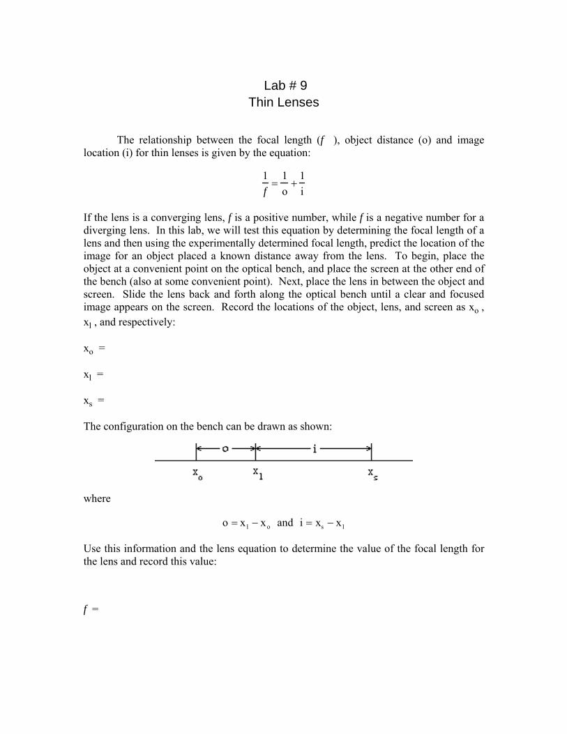
The configuration on the bench can be drawn as shown:

where

o = xl − xo and i = xs − xl

Use this information and the lens equation to determine the value of the focal length for the lens and record this value:

f =

Next, design a method to measure the focal length of a concave lens using the convex lens from the first part of this lab exercise. Describe this method below.

Using your method, measure the focal length of a concave lens, and record the number below.

Focal length = _______________________ .