Physically-based Surface Texture SynthesisUsing a Coupled Finite Element System

Chandrajit Bajaj1, Yongjie Zhang2, and Guoliang Xu3

1 Department of Computer Sciences and Institute for Computational Engineeringand Sciences, The University of Texas at Austin, USA. bajaj@cs.utexas.edu2 Department of Mechanical Engineering, Carnegie Mellon University, USA.

jessicaz@andrew.cmu.edu3 Institute of Computational Mathematics, Academy of Mathematics and System

Sciences, Chinese Academy of Sciences, China. xuguo@lsec.cc.ac.cn

Abstract. This paper describes a stable and robust finite element solverfor physically-based texture synthesis over arbitrary manifold surfaces.Our approach solves the reaction-diffusion equation coupled with ananisotropic diffusion equation over surfaces, using a Galerkin based finiteelement method (FEM). This method avoids distortions and discontinu-ities often caused by traditional texture mapping techniques, especiallyfor arbitrary manifold surfaces. Several varieties of textures are obtainedby selecting different values of control parameters in the governing dif-ferential equations, and furthermore enhanced quality textures are gen-erated by fairing out noise in input surface meshes.

Key words: texture synthesis, finite element method, reaction-diffusionequation, anisotropic diffusion.

1 Introduction

Texture mapping is an essential technique to map textures onto computer mod-els, but it usually introduces distortions or discontinuities. An alternate approachis to synthesize a texture directly on the surface of objects. The finite differencemethod (FDM) has been extended to generate patterns over surfaces, but theproblem of distortions or discontinuities still exist, and the results can be oftendivergent if non-suitable time steps or incorrect initial conditions are chosen.Here we use the finite element method (FEM) for the stable and robust solutionof reaction-diffusion partial differential equations (PDEs). These FEM solutionsallow for smooth and distortion free textures to be directly synthesized andvisualized on arbitrary surface manifolds.

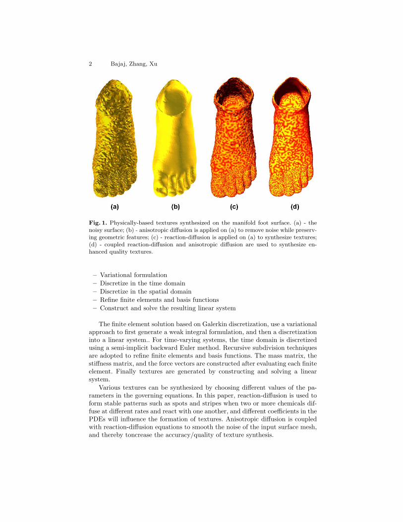
However when the input surface meshes are noisy, the textures synthesizedby FEM solutions are often equally noisy, and as shown in Figure 1. To correctthis, we couple an anisotropic diffusion PDE with the reaction-diffusion PDE’s toremove noise on the surface while preserving geometric features, and synthesizingsmooth textures at the same time. Enhanced and distortion-free textures aregenerated by using this coupled PDE system.

The main steps of our finite element texture synthesis approach are as follows:

2 Bajaj, Zhang, Xu

Fig. 1. Physically-based textures synthesized on the manifold foot surface. (a) - thenoisy surface; (b) - anisotropic diffusion is applied on (a) to remove noise while preserv-ing geometric features; (c) - reaction-diffusion is applied on (a) to synthesize textures;(d) - coupled reaction-diffusion and anisotropic diffusion are used to synthesize en-hanced quality textures.

– Variational formulation– Discretize in the time domain– Discretize in the spatial domain– Refine finite elements and basis functions– Construct and solve the resulting linear system

The finite element solution based on Galerkin discretization, use a variationalapproach to first generate a weak integral formulation, and then a discretizationinto a linear system.. For time-varying systems, the time domain is discretizedusing a semi-implicit backward Euler method. Recursive subdivision techniquesare adopted to refine finite elements and basis functions. The mass matrix, thestiffness matrix, and the force vectors are constructed after evaluating each finiteelement. Finally textures are generated by constructing and solving a linearsystem.

Various textures can be synthesized by choosing different values of the pa-rameters in the governing equations. In this paper, reaction-diffusion is used toform stable patterns such as spots and stripes when two or more chemicals dif-fuse at different rates and react with one another, and different coefficients in thePDEs will influence the formation of textures. Anisotropic diffusion is coupledwith reaction-diffusion equations to smooth the noise of the input surface mesh,and thereby toncrease the accuracy/quality of texture synthesis.

Physically-based Surface Texture Synthesis 3

The remainder of this paper is organized as follows: Section 2 summarizes pre-vious work related to texture synthesis, and finite element simulations; Section 3explains the algorithm of Galerkin based finite element method solutions; Section4 discusses the two coupled physical systems, reaction-diffusion and anisotropicdiffusion; The final section presents our conclusion and future work.

2 Previous Work

Previous work on texture synthesis with high visual or numerical accuracy fo-cuses on pattern generation and texture mapping, including statistical, non-parametric, as well as optimization-based techniques. In recent years, many tex-ture synthesis techniques have been developed.

Reaction-diffusion: The reaction-diffusion equations were proposed as amodel of biological pattern formation for texture synthesis. The traditionalreaction-diffusion systems are extended by allowing anisotropic and spatiallynon-uniform diffusion, as well as multiple competing directions of diffusion [4].There have been some attempts searching for different ways to generate textureson arbitrary surfaces based on FDM. Reaction-diffusion textures are generatedto match the geometry of an arbitrary polyhedral surface by creating a meshover a given surface and simulating the reaction-diffusion process directly on thismesh [5].

Texture Synthesis: During the past decade, many example-based texturesynthesis methods have been proposed, including parametric methods [12, 19, 6,7], non-parametric methods [13, 14, 20, 27, 28], optimization-based methods [15,10], and appearance-space texture synthesis [16]. In order to synthesize texturesover surfaces based on a given texture example, parametric methods attempt toconstruct a parametric model of the texture. Differently, non-parametric meth-ods grows the texture one pixel/patch at a time. Optimization-based methodsevolve the texture as a whole and improve the quality of the results. Besidestexture synthesis on surfaces, various techniques have also been developed forsolid texture synthesis [17, 18].

Anisotropic Diffusion: The isotropic diffusion method can remove noise,but blurs features such as edges and corners. In order to preserve features dur-ing the process of noise smoothing, anisotropic diffusion [22] was proposed byintroducing a diffusion tensor. Generally, a Gaussian filter is used to calculatethe anisotropic diffusion tensor before smoothing, but it also blurs features. Bi-lateral filtering [23], a nonlinear filter combining domain and range filtering, wasintroduced to solve this problem. Anisotropic diffusion can be used for fairingout noise both in surface meshes and functions defined on the surface [1, 24].

Simulation Using FEM: FEM has been used extensively in solving physi-cally based problems. A finite element solver, CHARMS (conforming, hierarchi-cal, adaptive refinement methods), constructs a framework for adaptive simula-tion by refining basis functions instead of refining elements [2]. An automatedprocedure [3] to generate a 3D finite element model of an individual patient’smandible with dental implants inserted was presented. Various methods of im-

4 Bajaj, Zhang, Xu

age processing, geometric modeling and finite element analysis were combinedand extended. The deformation field between 3D images was computed by locallyminimizing the sum of the squared differences between the images to be matched[11]. Nonlinear FEM using mass lumping was applied to produce a diagonal massmatrix that allows real time computation, and dynamic progressive meshes weregenerated to provide detailed information while minimizing computation [21].

3 Galerkin Based Finite Element Method

Textures can be generated by simulating physical phenomena, which are sim-plified into mathematical models represented by PDEs. Although FDM and itsvariants have been used extensively to solve PDEs, it is still challenging to syn-thesize textures directly over surfaces. FEM is a more stable and robust methodin solving PDEs over arbitrary manifold surfaces.

Given PDEs with the required property parameters and the correspondingboundary and initial conditions, FEM tends to solve the weak form of thesegoverning equations. The trial space and the test space are introduced. After thespatial and temporal discretization, each element is analyzed, and the recursivesubdivision is used to refine the elements and basis functions. In the Galerkinmethod, the same format is adopted to construct the trial function and the testfunction. The variational formulations are rewritten by plugging the trial and testfunctions into the weak form, and are modified with the boundary conditions.In the end, a simplified linear system is built by uniting all the finite elements,

Kx = b (1)

where x is the unknown vector. The matrix K and the vector b are calculated overthe surface domain, which is discretized into small elements such as triangles. Thetrial and test functions are defined in the same format as a linear combinationof basis functions, whose weights are elements of the unknown vector x. As aresult, textures are generated by solving the linear system.

3.1 Variational Formulation

A generalized PDE over surface Ω ⊂ R3 is shown in Equation (2), which canrepresent different physical phenomena by choosing corresponding variables andcoefficients, such as the reaction-diffusion and the anisotropic diffusion.

∂u

∂t= C0div(C1∇u) + C2u + C3 (2)

where div and ∇ are the divergence and the gradient operator over surface Ω(see [26] for their definitions), u represents different variables for various physicalproblems. u can be a scalar, for example, u is the concentration of a chemicalin the reaction-diffusion equations. u can also be a vector in R3 such as thegeometric position or function vectors at each vertex on Ω in the anisotropic

Physically-based Surface Texture Synthesis 5

diffusion equation. C0, C1, C2, and C3 are coefficients which can be functions ofu, or just constants. C1 could be a scalar or a 3× 3 matrix.

Suppose u, ν are selected from the trail space and the test space respectively,the inner product of u and ν is defined as follows,

(u, ν) =∫

Ω

uνdx. (3)

By using the Divergence Theorem and the Partial Integration Rule, Equation(2) can be written in a variational form as in Equation (4),(

C−10

∂u

∂t, ν

)= −(C1∇u,∇ν) + (C−1

0 C2u, ν)

+ (C−10 C3, ν). (4)

The variational form is the starting point for the following spatial and temporaldiscretizations.

3.2 Discretization

For time-varying systems, the variational form needs to be discretized in thetemporal space as well as in the spatial space. A semi-implicit backward Eulermethod is used for temporal discretization. For the spatial discretization, func-tions over the integration domain can be refined using the recursive subdivisionschemes [1].

Spatial Discretization: The variational problem in Equation (4) is dis-cretized in a function space which is defined by the limit of Loop’s recursivesubdivision. The function is locally parameterized in our finite element space,which is spanned by C1 smooth quartic box spline basis functions.

Temporal Discretization: For time-varying systems, we have to discretizeEquation (4) in the temporal space. Two issues need to be addressed for thetemporal discretization: the choice of the time step, and the decision of whichterm needs to analyzed implicitly and which term needs to be handled explicitly.Here a semi-implicit backward Euler discretization is chosen,

(un+1 − un

C0τ, ν

)= −(C1∇un+1,∇ν)

+ (C−10 C2u

n+1, ν) + (C−10 C3, ν), (5)

where τ is the time step, u at t = (n+1)τ is derived from u at t = nτ . Equation(5) is rewritten as follows,

(C−10 un+1, ν) + [(C1∇un+1,∇ν)− (C−1

0 C2un+1, ν)]τ

= (C−10 un, ν) + τ(C−1

0 C3, ν). (6)

6 Bajaj, Zhang, Xu

3.3 Element and Basis Refinement

For each vertex of a control mesh, its basis function is defined by the limit of theLoop’s subdivision for the zero control values everywhere except at itself whereit is one [1]. The recursive subdivision schemes are used to refine elements andbasis functions, and smooth surfaces are generated via a limit procedure of aniterative refinement. Here, an approximating algorithm proposed by Loop [8] isadopted. C2 limit surfaces are generated except for some extraordinary pointsat where C1 continuity is achieved.

If all the vertices of a triangle have a valence of 6, then the triangle is calledregular, otherwise it is irregular. A regular patch is controlled by twelve basisfunctions with explicit polynomial representations. For an irregular patch, themesh needs to be subdivided repeatedly until the parameter values of interestare inside a regular one [9].

The basis functions are defined by the same recursive scheme. For each vertexof a control mesh, we associate it with a basis function, which is defined asthe limit of the Loop’s subdivision from control value one at the vertex andcontrol value zero at every other vertices. Each triangle patch is defined locallyby only a few related basis functions. Triangles can be grouped according totheir vertex valences. All triangles with the same vertex valences have the sameset of related basis functions, which only need to be calculated once. Therefore,the computation costs in the numerical integration can be reduced.

3.4 Linear System Construction

The Galerkin approximation is applied to our variational formulation. The trialand test functions are defined in the same format - a linear combination of basisfunctions,

u =N∑

i=1

uiφi, ν =N∑

i=1

νiφi. (7)

Substitute Equation (7) into Equation (6), and rewrite it for each νj , we obtain

(M + τL)un+1 = Mun + τF, (8)

where the mass matrix M , the stiffness matrix L, and the force vector F can becalculated as follows,

Mij = (C−10 φi, φj), (9)

Lij = (C1∇φi,∇φj)− (C−10 C2φi, φj), (10)

Fj = (C−10 C3, φj). (11)

The resulting linear system arising in each time step τ can be solved by a pre-conditioned conjugate gradient method. After each ui (i = 1, ..., N) is calculated,we can obtain u by substituting them back into Equation (7).

Physically-based Surface Texture Synthesis 7

4 A Coupled System of Reaction-Diffusion andAnisotropic Diffusion

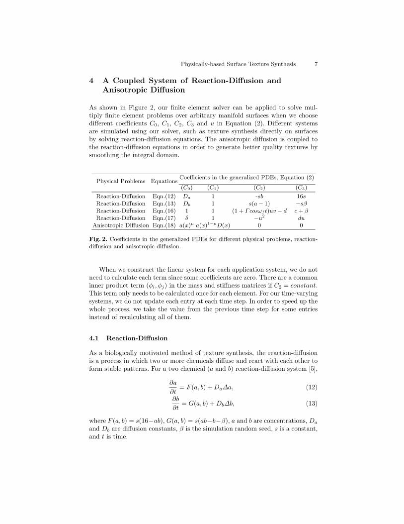
As shown in Figure 2, our finite element solver can be applied to solve mul-tiply finite element problems over arbitrary manifold surfaces when we choosedifferent coefficients C0, C1, C2, C3 and u in Equation (2). Different systemsare simulated using our solver, such as texture synthesis directly on surfacesby solving reaction-diffusion equations. The anisotropic diffusion is coupled tothe reaction-diffusion equations in order to generate better quality textures bysmoothing the integral domain.

Physical Problems EquationsCoefficients in the generalized PDEs, Equation (2)

(C0) (C1) (C2) (C3)

Reaction-Diffusion Eqn.(12) Da 1 -sb 16sReaction-Diffusion Eqn.(13) Db 1 s(a− 1) −sβReaction-Diffusion Eqn.(16) 1 1 (1 + Γcosωf t)uv − d c + βReaction-Diffusion Eqn.(17) δ 1 −u2 du

Anisotropic Diffusion Eqn.(18) a(x)µ a(x)1−µD(x) 0 0

Fig. 2. Coefficients in the generalized PDEs for different physical problems, reaction-diffusion and anisotropic diffusion.

When we construct the linear system for each application system, we do notneed to calculate each term since some coefficients are zero. There are a commoninner product term (φi, φj) in the mass and stiffness matrices if C2 = constant.This term only needs to be calculated once for each element. For our time-varyingsystems, we do not update each entry at each time step. In order to speed up thewhole process, we take the value from the previous time step for some entriesinstead of recalculating all of them.

4.1 Reaction-Diffusion

As a biologically motivated method of texture synthesis, the reaction-diffusionis a process in which two or more chemicals diffuse and react with each other toform stable patterns. For a two chemical (a and b) reaction-diffusion system [5],

∂a

∂t= F (a, b) + Da∆a, (12)

∂b

∂t= G(a, b) + Db∆b, (13)

where F (a, b) = s(16−ab), G(a, b) = s(ab−b−β), a and b are concentrations, Da

and Db are diffusion constants, β is the simulation random seed, s is a constant,and t is time.

8 Bajaj, Zhang, Xu

In this paper, FEM is adopted to solve the PDEs. System (12-13) is weakenedby using the divergence theorem and the partial integration, then both trialfunctions (a and b) and the test function (ν) are discretized in the same format.The reformulated variational form can be written as,

(an+1, ν) + (sτbnan+1, ν) + (Daτ∇an+1,∇ν)= (an, ν) + (16sτ, ν), (14)

(bn+1, ν) − (sτanbn+1, ν) + (Dbτ∇bn+1,∇ν)+ (sτbn+1, ν) = (bn, ν)− (sβτ, ν), (15)

where τ is the time step, and an is the concentration at time t = nτ . Equation(14-15) can be rewritten into a linear system in Equation (8). The mass matrix,the stiffness matrix and the force vector of Equation (14) are as follows,

Mij = (D−1a φi, φj),

Lij = (∇φi,∇φj)− (sbD−1a φi, φj),

Fj = (16sD−1a , φj).

Similarly, the mass matrix, the stiffness matrix and the force vector of Equation(15) are as follows,

Mij = (D−1b φi, φj),

Lij = (∇φi,∇φj) + (saD−1b φi, φj)− (sD−1

b φi, φj),Fj = −(sβD−1

b , φj).

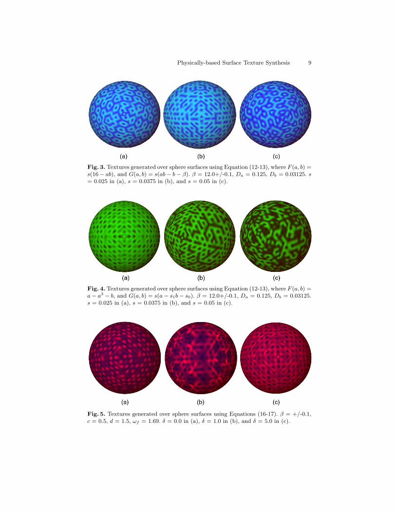
Given the initial values a = b = 4.0, the concentrations of chemical a and b canbe obtained at each time step iteratively. Specifically, for each temporal step,the system consisting of equations (14)-(15) is solved iteratively, until a and bachieve their stable states. Figure 3 and 4 show different patterns generated overa sphere surface. Spot and stripe patterns can be controlled by selecting differentvalues of the parameters.

Additionally as shown in Figure 5, we used the same variational algorithmto solve another reaction-diffusion equations,

∂u

∂t= c + β − du + (1 + Γcosωf t)u2v + ∆u, (16)

∂v

∂t= du− u2v + δ∆v. (17)

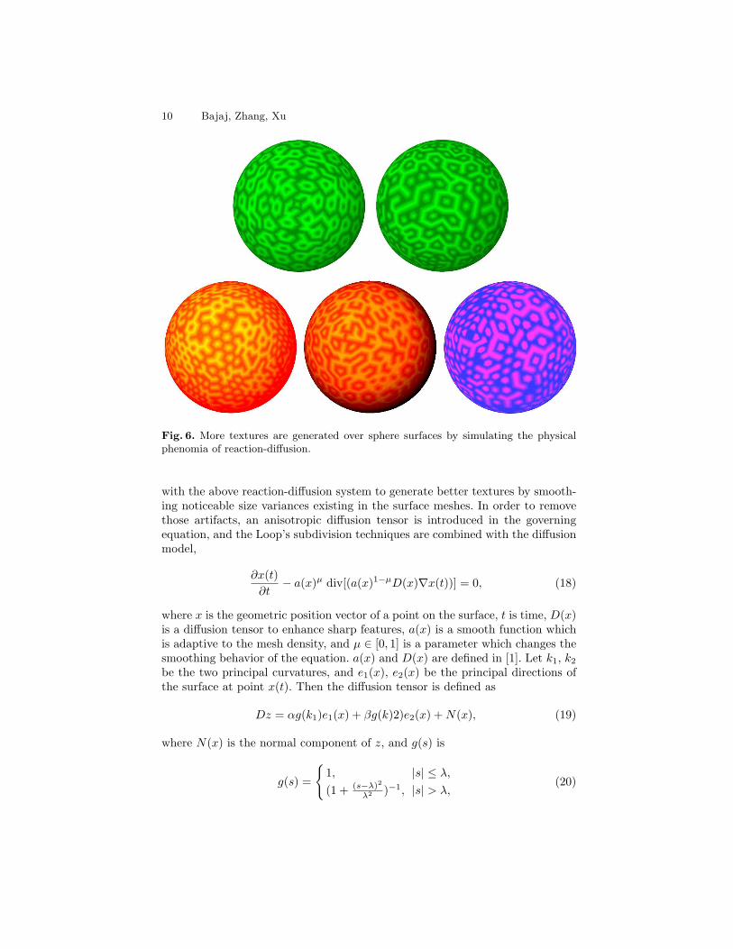
Figure 6 shows more textures generated by choosing different parameters inthe physical phenomena of reaction-diffusion, Equation (12-13) or (16-17).

4.2 Anisotropic Diffusion

If F (a, b) = 0, then Equations (12) turns into an isotropic diffusion equation.Another kind of diffusion problem is anisotropic diffusion, which usually couples

Physically-based Surface Texture Synthesis 9

Fig. 3. Textures generated over sphere surfaces using Equation (12-13), where F (a, b) =s(16− ab), and G(a, b) = s(ab− b− β). β = 12.0+/-0.1, Da = 0.125, Db = 0.03125. s= 0.025 in (a), s = 0.0375 in (b), and s = 0.05 in (c).

Fig. 4. Textures generated over sphere surfaces using Equation (12-13), where F (a, b) =a− a3 − b, and G(a, b) = s(a− s1b− s0). β = 12.0+/-0.1, Da = 0.125, Db = 0.03125.s = 0.025 in (a), s = 0.0375 in (b), and s = 0.05 in (c).

Fig. 5. Textures generated over sphere surfaces using Equations (16-17). β = +/-0.1,c = 0.5, d = 1.5, ωf = 1.69. δ = 0.0 in (a), δ = 1.0 in (b), and δ = 5.0 in (c).

10 Bajaj, Zhang, Xu

Fig. 6. More textures are generated over sphere surfaces by simulating the physicalphenomia of reaction-diffusion.

with the above reaction-diffusion system to generate better textures by smooth-ing noticeable size variances existing in the surface meshes. In order to removethose artifacts, an anisotropic diffusion tensor is introduced in the governingequation, and the Loop’s subdivision techniques are combined with the diffusionmodel,

∂x(t)∂t

− a(x)µ div[(a(x)1−µD(x)∇x(t))] = 0, (18)

where x is the geometric position vector of a point on the surface, t is time, D(x)is a diffusion tensor to enhance sharp features, a(x) is a smooth function whichis adaptive to the mesh density, and µ ∈ [0, 1] is a parameter which changes thesmoothing behavior of the equation. a(x) and D(x) are defined in [1]. Let k1, k2

be the two principal curvatures, and e1(x), e2(x) be the principal directions ofthe surface at point x(t). Then the diffusion tensor is defined as

Dz = αg(k1)e1(x) + βg(k)2)e2(x) + N(x), (19)

where N(x) is the normal component of z, and g(s) is

g(s) =

1, |s| ≤ λ,

(1 + (s−λ)2

λ2 )−1, |s| > λ,(20)

Physically-based Surface Texture Synthesis 11

λ is a given parameter which detects sharp features. After the spatial and timediscretization of the weak form, Equation (18) can be rewritten as follows,

(a(xn)−µxn+1, ν) + τ(a(xn)1−µD(xn)∇xn+1,∇ν)= (a(xn)−µxn, ν), (21)

where ν is the test function, τ is the time step, and n is the step number. Themass matrix, the stiffness matrix and the force vector are as follow,

Mij = (a(x)−µφi, φj),Lij = (a(x)1−µD(x)∇φi,∇φj),Fj = 0.

Our finite element solver can smooth both geometric positions and functionvalues of each vertex on the surface. Anisotropic diffusion is used to improvethe quality of the synthesized textures by denoising the surface meshes whilepreserving geometric features. Figure 1(a-b) show one example.

4.3 A Coupled System

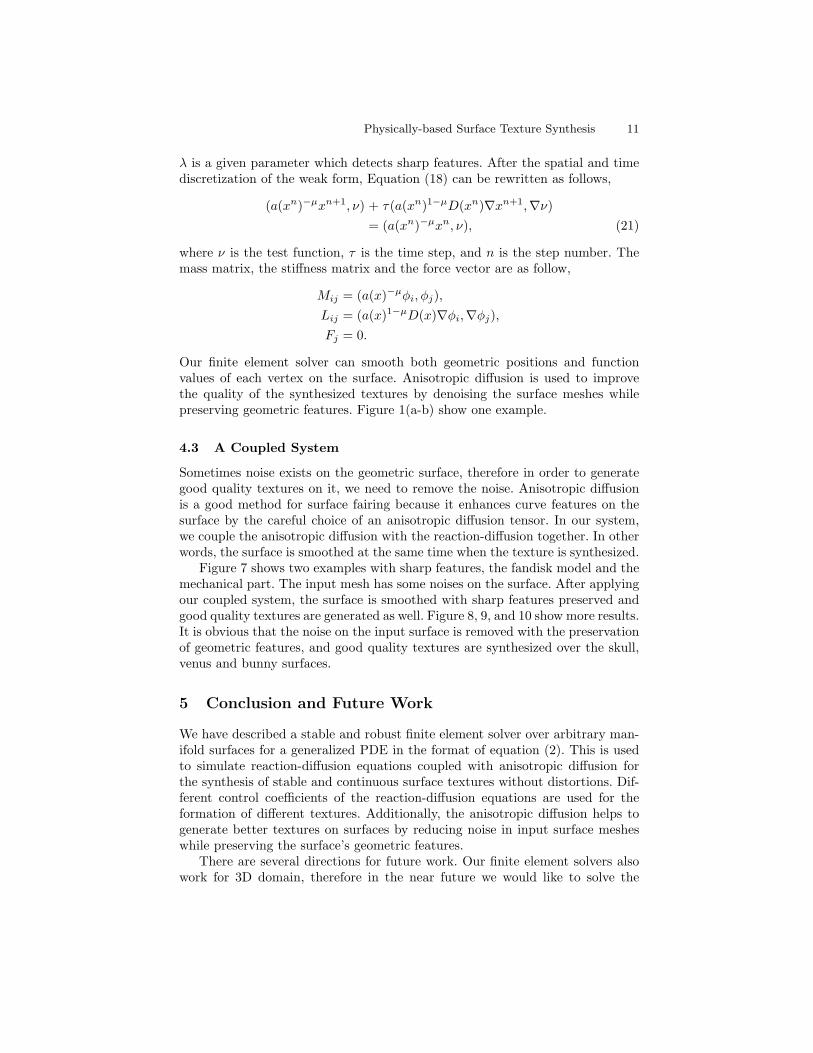
Sometimes noise exists on the geometric surface, therefore in order to generategood quality textures on it, we need to remove the noise. Anisotropic diffusionis a good method for surface fairing because it enhances curve features on thesurface by the careful choice of an anisotropic diffusion tensor. In our system,we couple the anisotropic diffusion with the reaction-diffusion together. In otherwords, the surface is smoothed at the same time when the texture is synthesized.

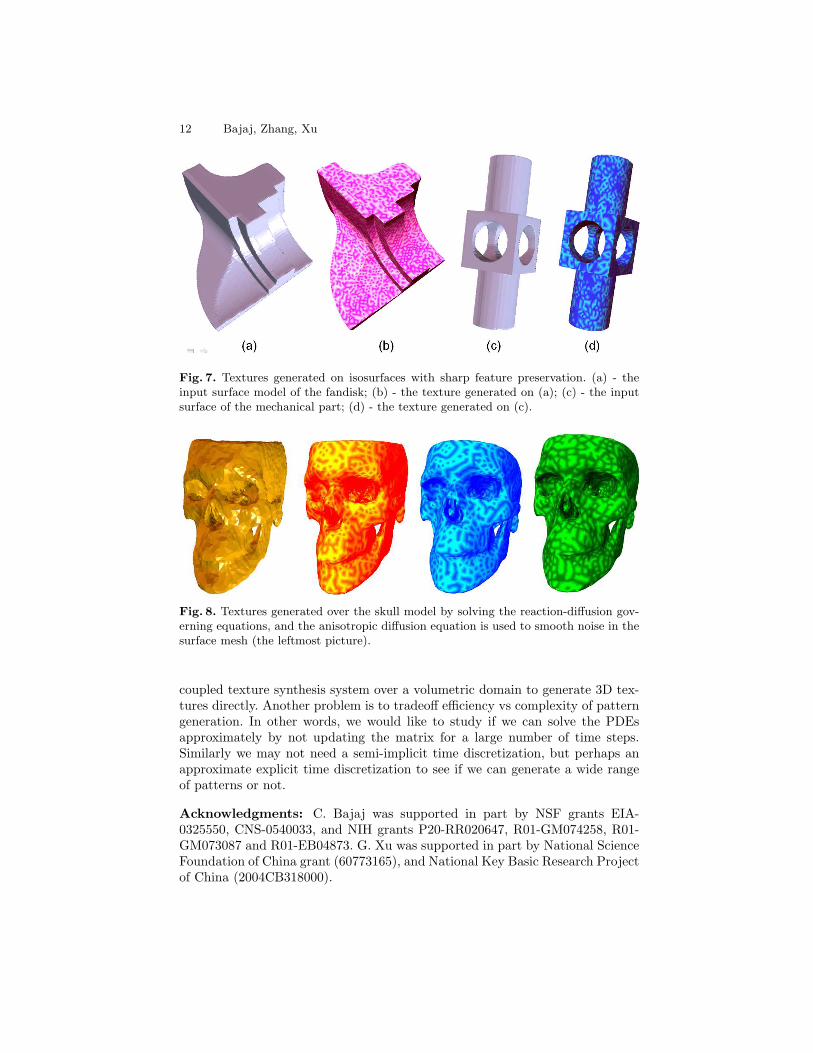
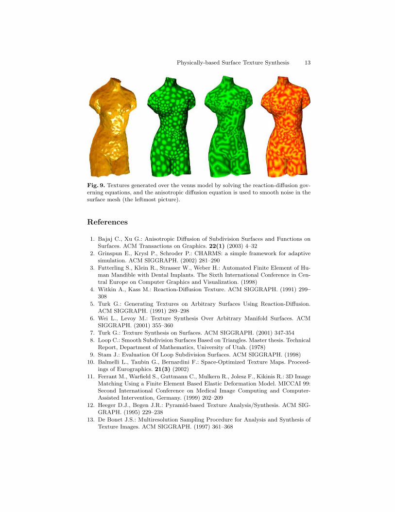
Figure 7 shows two examples with sharp features, the fandisk model and themechanical part. The input mesh has some noises on the surface. After applyingour coupled system, the surface is smoothed with sharp features preserved andgood quality textures are generated as well. Figure 8, 9, and 10 show more results.It is obvious that the noise on the input surface is removed with the preservationof geometric features, and good quality textures are synthesized over the skull,venus and bunny surfaces.

5 Conclusion and Future Work

We have described a stable and robust finite element solver over arbitrary man-ifold surfaces for a generalized PDE in the format of equation (2). This is usedto simulate reaction-diffusion equations coupled with anisotropic diffusion forthe synthesis of stable and continuous surface textures without distortions. Dif-ferent control coefficients of the reaction-diffusion equations are used for theformation of different textures. Additionally, the anisotropic diffusion helps togenerate better textures on surfaces by reducing noise in input surface mesheswhile preserving the surface’s geometric features.

There are several directions for future work. Our finite element solvers alsowork for 3D domain, therefore in the near future we would like to solve the

12 Bajaj, Zhang, Xu

Fig. 7. Textures generated on isosurfaces with sharp feature preservation. (a) - theinput surface model of the fandisk; (b) - the texture generated on (a); (c) - the inputsurface of the mechanical part; (d) - the texture generated on (c).

Fig. 8. Textures generated over the skull model by solving the reaction-diffusion gov-erning equations, and the anisotropic diffusion equation is used to smooth noise in thesurface mesh (the leftmost picture).

coupled texture synthesis system over a volumetric domain to generate 3D tex-tures directly. Another problem is to tradeoff efficiency vs complexity of patterngeneration. In other words, we would like to study if we can solve the PDEsapproximately by not updating the matrix for a large number of time steps.Similarly we may not need a semi-implicit time discretization, but perhaps anapproximate explicit time discretization to see if we can generate a wide rangeof patterns or not.

Acknowledgments: C. Bajaj was supported in part by NSF grants EIA-0325550, CNS-0540033, and NIH grants P20-RR020647, R01-GM074258, R01-GM073087 and R01-EB04873. G. Xu was supported in part by National ScienceFoundation of China grant (60773165), and National Key Basic Research Projectof China (2004CB318000).

Physically-based Surface Texture Synthesis 13

Fig. 9. Textures generated over the venus model by solving the reaction-diffusion gov-erning equations, and the anisotropic diffusion equation is used to smooth noise in thesurface mesh (the leftmost picture).

References

1. Bajaj C., Xu G.: Anisotropic Diffusion of Subdivision Surfaces and Functions onSurfaces. ACM Transactions on Graphics. 22(1) (2003) 4–32

2. Grinspun E., Krysl P., Schroder P.: CHARMS: a simple framework for adaptivesimulation. ACM SIGGRAPH. (2002) 281–290

3. Futterling S., Klein R., Strasser W., Weber H.: Automated Finite Element of Hu-man Mandible with Dental Implants. The Sixth International Conference in Cen-tral Europe on Computer Graphics and Visualization. (1998)

4. Witkin A., Kass M.: Reaction-Diffusion Texture. ACM SIGGRAPH. (1991) 299–308

5. Turk G.: Generating Textures on Arbitrary Surfaces Using Reaction-Diffusion.ACM SIGGRAPH. (1991) 289–298

6. Wei L., Levoy M.: Texture Synthesis Over Arbitrary Manifold Surfaces. ACMSIGGRAPH. (2001) 355–360

7. Turk G.: Texture Synthesis on Surfaces. ACM SIGGRAPH. (2001) 347-354

8. Loop C.: Smooth Subdivision Surfaces Based on Triangles. Master thesis. TechnicalReport, Department of Mathematics, University of Utah. (1978)

9. Stam J.: Evaluation Of Loop Subdivision Surfaces. ACM SIGGRAPH. (1998)

10. Balmelli L., Taubin G., Bernardini F.: Space-Optimized Texture Maps. Proceed-ings of Eurographics. 21(3) (2002)

11. Ferrant M., Warfield S., Guttmann C., Mulkern R., Jolesz F., Kikinis R.: 3D ImageMatching Using a Finite Element Based Elastic Deformation Model. MICCAI 99:Second International Conference on Medical Image Computing and Computer-Assisted Intervention, Germany. (1999) 202–209

12. Heeger D.J., Begen J.R.: Pyramid-based Texture Analysis/Synthesis. ACM SIG-GRAPH. (1995) 229–238

13. De Bonet J.S.: Multiresolution Sampling Procedure for Analysis and Synthesis ofTexture Images. ACM SIGGRAPH. (1997) 361–368

14 Bajaj, Zhang, Xu

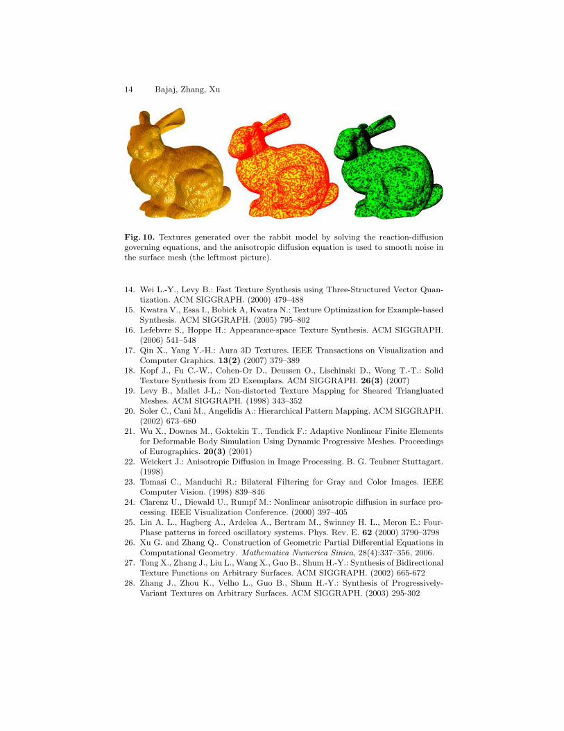
Fig. 10. Textures generated over the rabbit model by solving the reaction-diffusiongoverning equations, and the anisotropic diffusion equation is used to smooth noise inthe surface mesh (the leftmost picture).

14. Wei L.-Y., Levy B.: Fast Texture Synthesis using Three-Structured Vector Quan-tization. ACM SIGGRAPH. (2000) 479–488

15. Kwatra V., Essa I., Bobick A, Kwatra N.: Texture Optimization for Example-basedSynthesis. ACM SIGGRAPH. (2005) 795–802

16. Lefebvre S., Hoppe H.: Appearance-space Texture Synthesis. ACM SIGGRAPH.(2006) 541–548

17. Qin X., Yang Y.-H.: Aura 3D Textures. IEEE Transactions on Visualization andComputer Graphics. 13(2) (2007) 379–389

18. Kopf J., Fu C.-W., Cohen-Or D., Deussen O., Lischinski D., Wong T.-T.: SolidTexture Synthesis from 2D Exemplars. ACM SIGGRAPH. 26(3) (2007)

19. Levy B., Mallet J-L.: Non-distorted Texture Mapping for Sheared TriangluatedMeshes. ACM SIGGRAPH. (1998) 343–352

20. Soler C., Cani M., Angelidis A.: Hierarchical Pattern Mapping. ACM SIGGRAPH.(2002) 673–680

21. Wu X., Downes M., Goktekin T., Tendick F.: Adaptive Nonlinear Finite Elementsfor Deformable Body Simulation Using Dynamic Progressive Meshes. Proceedingsof Eurographics. 20(3) (2001)

22. Weickert J.: Anisotropic Diffusion in Image Processing. B. G. Teubner Stuttagart.(1998)

23. Tomasi C., Manduchi R.: Bilateral Filtering for Gray and Color Images. IEEEComputer Vision. (1998) 839–846

24. Clarenz U., Diewald U., Rumpf M.: Nonlinear anisotropic diffusion in surface pro-cessing. IEEE Visualization Conference. (2000) 397–405

25. Lin A. L., Hagberg A., Ardelea A., Bertram M., Swinney H. L., Meron E.: Four-Phase patterns in forced oscillatory systems. Phys. Rev. E. 62 (2000) 3790–3798

26. Xu G. and Zhang Q.. Construction of Geometric Partial Differential Equations inComputational Geometry. Mathematica Numerica Sinica, 28(4):337–356, 2006.

27. Tong X., Zhang J., Liu L., Wang X., Guo B., Shum H.-Y.: Synthesis of BidirectionalTexture Functions on Arbitrary Surfaces. ACM SIGGRAPH. (2002) 665-672

28. Zhang J., Zhou K., Velho L., Guo B., Shum H.-Y.: Synthesis of Progressively-Variant Textures on Arbitrary Surfaces. ACM SIGGRAPH. (2003) 295-302