PHYSICAL REVIEW E 102, 022134 (2020)

Stochastic resetting and the mean-field dynamics of focal adhesions

Paul C. BressloffDepartment of Mathematics, University of Utah Salt Lake City, Utah 84112, USA

(Received 20 May 2020; accepted 12 August 2020; published 24 August 2020)

In this paper we investigate the effects of diffusion on the dynamics of a single focal adhesion at the leadingedge of a crawling cell by considering a simplified model of sliding friction. Using a mean-field approximation,we derive an effective single-particle system that can be interpreted as an overdamped Brownian particle withspatially dependent stochastic resetting. We then use renewal and path-integral methods from the theory ofstochastic resetting to calculate the mean sliding velocity under the combined action of diffusion, active forces,viscous drag, and elastic forces generated by the adhesive bonds. Our analysis suggests that the inclusion ofdiffusion can sharpen the response to changes in the effective stiffness of the adhesion bonds. This is consistentwith the hypothesis that force fluctuations could play a role in mechanosensing of the local microenvironment.

DOI: 10.1103/PhysRevE.102.022134

I. INTRODUCTION

Tissue cell migration along a substrate such as the extra-cellular matrix (ECM) requires adhesion forces between thecell and substrate. Adhesion is necessary in order to balancepropulsive forces at the leading edge of the cell that are gener-ated by actin polymerization and contractile forces at the rearthat are driven by myosin II motors [1,2]. Adhesive forces aremediated by transmembrane receptors (integrins) [3], whichform one layer of a large multiprotein complex known as afocal adhesion (FA), see Fig. 1(a). More specifically, integrinsare heterodimeric proteins whose extracellular domains attachto the substrate, while their intracellular domains act as bind-ing sites for various submembrane proteins, resulting in theformation of the plaque. The plaque, which consists of morethan 50 different types of protein, links the integrin layer to theactin cytoskeleton, and plays a role in intracellular signalingand force transduction.

Experimental studies of migratory cells suggests that atthe leading edge, the FA acts like a molecular clutch [4–8].That is, for high adhesion or drag, the retrograde flow of actinis slow and polymerization results in a net protrusion—theclutch is in “drive.” On the other hand, if adhesion is weak,then retrograde flow can cancel the polymerization and theactin network treadmills, i.e., the clutch is in “neutral.” Thedynamical interplay between retrograde flow and the assem-bly and disassembly of focal adhesions leads to a number ofbehaviors that are characteristic of physical systems involvingfriction at moving interfaces [9–11]. These include biphasicbehavior in the velocity-stress relation and stick-slip motion.The latter is a form of jerky motion, whereby a system spendsmost of its time in the “stuck” state and a relatively shorttime in the “slip” state. Various insights into the molecularclutch mechanism and its role in substrate stiffness-dependentmigration have been obtained using simple stochastic models[12–17]. Such models can capture the biphasic stick-slip forcevelocity relation and establish the existence of an optimalsubstrate stiffness that is sensitive to the operating parametersof the molecular clutch.

There is growing experimental evidence that integrins orFAs also act as biochemical mechanosensors of the localmicroenvironment such as the rigidity and composition ofthe ECM [18,19]. Rigidity sensors are thought to play animportant role in guiding cell migration, in particular, theability of cells to migrate toward areas of higher ECM rigidityvia a process known as durotaxis [20–22]. Physiologicalprocess involving durotaxis include stem cell differentiation,wound healing, development of the nervous system, and theproliferation of certain cancers (see the cited references). Inorder to move along a rigidity gradient, there has to be somemechanism for constantly surveying variations in the stiffnesslandscape of the ECM within the cellular microenvironment.Recently, high-resolution traction force microscopy has beenused to characterize the nanoscale spatiotemporal dynamicsof forces exerted by FAs during durotaxis [23]. These andother studies have revealed that mature FAs exhibit internalfluctuations in their traction forces, suggestive of repeatedtugging on the ECM. This has led to the hypothesis thatrepeated FA tugging on the ECM provides a means of reg-ularly testing the local ECM rigidity landscape over time.At least three different mechanisms for generating tractionforce fluctuations have been proposed [21]: Fluctuations inmyosin contractility, fluctuations in the mechanics of actinstress fibers, and fluctuations in the FA molecular clutch itself.One important observation is that temporal variations arelocal to a single FA. That is, although neighboring FAs aremechanically coupled to each other via the actin cytoskeleton,their force fluctuations are uncorrelated [23].

The role of FAs in cell motility is related to the moregeneral physical problem of understanding friction at mov-ing interfaces (tribology). Some of the generic aspects ofmolecular bonding at sliding interfaces has been investigatedin a stochastic model of single FA dynamics introduced bySabass and Schwarz [13]. A schematic diagram of the modelis shown in Fig. 1(b). The local stress fibers connected tothe FA are treated as a rigid slider that moves over thesubstrate (retrograde flow) under the action of a constantdriving force F . The latter represents the combined effects

2470-0045/2020/102(2)/022134(13) 022134-1 ©2020 American Physical Society

PAUL C. BRESSLOFF PHYSICAL REVIEW E 102, 022134 (2020)

substrate

integrin layer

plaque proteins

actin stress fibers

driving force F

elastic force

viscous force

(a)

(b)

FIG. 1. (a) Schematic diagram of a FA. A layer of integrinreceptors is attached to the ECM substrate and a submembraneplaque consisting of multiple proteins mediates force transmissionand signaling between the integrin layer and actin stress fibers. Actinpolymerization and the actomyosin contractile machinery generateforces that affect mechanosensitive proteins in the various com-ponents of the FA. (b) Simplified model of sliding friction. Thedriving force F for sliding is balanced by elastic adhesive forces andvelocity-dependent viscous forces.

of contractile forces exerted by myosin motors at the trailingedge of the cell and actin polymerization at the leading edge.The force F is balanced by two time-dependent forces: anelastic force due to integrins that are stochastically bound atthe interface and a viscous friction force ξv, where v is thesliding velocity and ξ is a friction coefficient. When a bondis attached to the cytoskeleton it stretches at the velocity v,but its extension x is immediately reset to zero whenever itunbinds. The latter occurs at an x-dependent rate koff (x). Thebond subsequently rebinds at a constant binding rate kon. Thebonds are coupled due to the fact that the sliding velocitydepends on the sum of the elastic forces generated by theclosed bonds. However, using a mean-field approximation,one can derive an effective single-bond dynamics with aconstant sliding velocity that is determined self-consistentlyfrom the single-bond statistics [13]. The mean-field modelwas shown to exhibit biphasic frictional behavior as a functionof ξ , consistent with Monte Carlo simulations.

In this paper we extend the model from Ref. [13] by addinga stochastic component �F = σ�W (t ) to the driving force,where �W (t ) is a Gaussian random variable (Wiener process)and σ is the noise strength. In terms of the application toFA adhesions dynamics, �F could represent fluctuations inmyosin contractility or actin mechanics. The inclusion of anoise term is consistent with the Einstein relation, whichimplies that the noise strength and friction coefficient ξ arerelated according to σ = ξ

√2D with Dξ = kBT . Here D is

the diffusion coefficient of the slider, T is temperature, and kB

is the Boltzmann constant. From a mathematical perspective,the fluctuating force can be accounted for by the additionof second-order spatial derivative terms to the Chapman-Kolmogorov master equation analyzed in Ref. [13]. Indeed,this extension was briefly mentioned by the authors. However,

such terms considerably complicate the analysis. In this paperwe show how progress can be made by mapping the single-bond dynamics onto an equivalent single-particle system withstochastic resetting.

Stochastic resetting has generated considerable interestwithin the context of optimal search processes. A canoni-cal example is a Brownian particle whose position is resetrandomly in time at a constant rate r (Poissonian resetting)to some fixed point Xr , which could be its initial position.This system exhibits two of the major features observedin more complex models: (i) convergence to a nontrivialnonequilibrium stationary state (NESS) and (ii) the mean timefor a Brownian particle to find a hidden target is finite andhas an optimal value as a function of the resetting rate r[24–26]. There have been numerous studies of more generalstochastic processes with both Poissonian and non-Poissonianresetting, memory effects, and spatially extended systems, seethe recent review [27] and references therein. In the particularcase of bond dynamics, the extension of a bond represents theposition of a particle that resets to the origin at a spatiallydependent resetting rate r(x) = koff (x), after which it remainsat the origin for a refractory period of mean duration k−1

on .If Brownian motion of the sliding cytoskeleton is included,then the system behaves as an overdamped Brownian particlemoving in a potential well [28] and subject to spatially depen-dent resetting [29] and a refractory period [30]. The advantageof formulating bond dynamics in terms of a process withstochastic resetting is that one can apply various analyticaltools, including renewal theory and path integral methods.

The structure of the paper is as follows. The basic slidingfriction model is introduced in Sec. II, which takes the formof a stochastic hybrid system that couples the continuousdynamics of bond stretching with the Markov chain forbinding and unbinding. We also construct the differentialChapman-Kolmogorov (CK) equation for the evolution ofthe corresponding joint probability density. In Sec. III weconsider the case of a single bond and show how the resultingsystem can be reinterpreted in terms of an overdamped Brow-nian particle with spatially dependent stochastic resetting. Wederive a general expression for the steady-state density of thesingle-particle CK equation by extending the renewal theoryof Ref. [29]. We then calculate the density in the case ofconstant sliding velocity v0 and a parabolic resetting function.In Sec. IV, we show how the multibond system can be reducedto the single-particle model of Sec. III using a mean-fieldapproximation along analogous lines to Ref. [13]. This yieldsan equation relating v0 to the mean traction force. We thusshow how diffusion can sharpen the response to changes inthe effective stiffness of the adhesion bonds. This is consistentwith the hypothesis that force fluctuations could play a role inmechanosensing of the local microenvironment.

II. STOCHASTIC MODEL OF SLIDING FRICTION

We begin by describing the model of sliding friction con-sidered in Ref. [13] and illustrated in Fig. 1(b). Suppose thatthe FA is of constant size so that there is a fixed maximalnumber of N assembled bonds. Each bond, i = 1, . . . , N , canbe in one of two states denoted by qi(t ) ∈ {0, 1}, with thebond closed (open) if qi(t ) = 1 [qi(t ) = 0]. The closed bonds

022134-2

STOCHASTIC RESETTING AND THE MEAN-FIELD … PHYSICAL REVIEW E 102, 022134 (2020)

elasticforce

ΔX ΔX

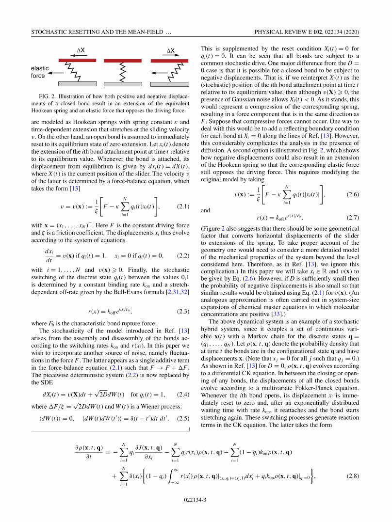
FIG. 2. Illustration of how both positive and negative displace-ments of a closed bond result in an extension of the equivalentHookean spring and an elastic force that opposes the driving force.

are modeled as Hookean springs with spring constant κ andtime-dependent extension that stretches at the sliding velocityv. On the other hand, an open bond is assumed to immediatelyreset to its equilibrium state of zero extension. Let xi(t ) denotethe extension of the ith bond attachment point at time t relativeto its equilibrium value. Whenever the bond is attached, itsdisplacement from equilibrium is given by dxi(t ) = dX (t ),where X (t ) is the current position of the slider. The velocity v

of the latter is determined by a force-balance equation, whichtakes the form [13]

v = v(x) := 1

ξ

[F − κ

N∑i=1

qi(t )xi(t )

], (2.1)

with x = (x1, . . . , xN )�. Here F is the constant driving forceand ξ is a friction coefficient. The displacements xi thus evolveaccording to the system of equations

dxi

dt= v(x) if qi(t ) = 1, xi = 0 if qi(t ) = 0, (2.2)

with i = 1, . . . , N and v(x) � 0. Finally, the stochasticswitching of the discrete state qi(t ) between the values 0,1is determined by a constant binding rate kon and a stretch-dependent off-rate given by the Bell-Evans formula [2,31,32]

r(x) = koff eκx/Fb, (2.3)

where Fb is the characteristic bond rupture force.The stochasticity of the model introduced in Ref. [13]

arises from the assembly and disassembly of the bonds ac-cording to the switching rates kon and r(xi ). In this paper wewish to incorporate another source of noise, namely fluctua-tions in the force F . The latter appears as a single additive termin the force-balance equation (2.1) such that F → F + �F .The piecewise deterministic system (2.2) is now replaced bythe SDE

dXi(t ) = v(X)dt +√

2DdW (t ) for qi(t ) = 1, (2.4)

where �F/ξ = √2DdW (t ) and W (t ) is a Wiener process:

〈dW (t )〉 = 0, 〈dW (t )dW (t ′)〉 = δ(t − t ′)dt dt ′. (2.5)

This is supplemented by the reset condition Xi(t ) = 0 forqi(t ) = 0. It can be seen that all bonds are subject to acommon stochastic drive. One major difference from the D =0 case is that it is possible for a closed bond to be subject tonegative displacements. That is, if we reinterpret Xi(t ) as the(stochastic) position of the ith bond attachment point at time trelative to its equilibrium value, then although v(X) � 0, thepresence of Gaussian noise allows Xi(t ) < 0. As it stands, thiswould represent a compression of the corresponding spring,resulting in a force component that is in the same direction asF . Suppose that compressive forces cannot occur. One way todeal with this would be to add a reflecting boundary conditionfor each bond at Xi = 0 along the lines of Ref. [13]. However,this considerably complicates the analysis in the presence ofdiffusion. A second option is illustrated in Fig. 2, which showshow negative displacements could also result in an extensionof the Hookean spring so that the corresponding elastic forcestill opposes the driving force. This requires modifying theoriginal model by taking

v(x) := 1

ξ

[F − κ

N∑i=1

qi(t )|xi(t )|], (2.6)

andr(x) = koff e

κ|x|/Fb . (2.7)

(Figure 2 also suggests that there should be some geometricalfactor that converts horizontal displacements of the sliderto extensions of the spring. To take proper account of thegeometry one would need to consider a more detailed modelof the mechanical properties of the system beyond the levelconsidered here. Therefore, as in Ref. [13], we ignore thiscomplication.) In this paper we will take xi ∈ R and v(x) tobe given by Eq. (2.6). However, if D is sufficiently small thenthe probability of negative displacements is also small so thatsimilar results would be obtained using Eq. (2.1) for v(x). (Ananalogous approximation is often carried out in system-sizeexpansions of chemical master equations in which molecularconcentrations are positive [33].)

The above dynamical system is an example of a stochastichybrid system, since it couples a set of continuous vari-able x(t ) with a Markov chain for the discrete states q =(q1, . . . , qN ). Let ρ(x, t, q) denote the probability density thatat time t the bonds are in the configurational state q and havedisplacements x. (Note that x j = 0 for all j such that q j = 0.)As shown in Ref. [13] for D = 0, ρ(x, t, q) evolves accordingto a differential CK equation. In between the closing or open-ing of any bonds, the displacements of all the closed bondsevolve according to a multivariate Fokker-Planck equation.Whenever the ith bond opens, its displacement xi is imme-diately reset to zero and, after an exponentially distributedwaiting time with rate kon, it reattaches and the bond startsstretching again. These switching processes generate reactionterms in the CK equation. The latter takes the form

∂ρ(x, t, q)

∂t= −

N∑i=1

qi∂J (x, t, q)

∂xi−

N∑i=1

qir(xi )ρ(x, t, q) −N∑

i=1

(1 − qi )konρ(x, t, q)

+N∑

i=1

δ(xi )

{(1 − qi )

∫ ∞

−∞r(x′

i )ρ(x, t, q)|(xi,qi )=(x′i ,1)dx′

i + qikonρ(x, t, q)|qi=0

}, (2.8)

022134-3

PAUL C. BRESSLOFF PHYSICAL REVIEW E 102, 022134 (2020)

where

J (x, t, q) = −DN∑

j=1

q j∂ρ(x, t, q)

∂x j+ v(x)ρ(x, t, q). (2.9)

The first summation on the right-hand side of Eq. (2.8)represent the advection-diffusion of closed bonds in betweenswitching events. Note that the diffusion matrix is Di j = D forall i, j rather than the standard diagonal matrix Di j = Dδi, j ,which is due to the fact that all bonds are driven by a com-mon Brownian motion. The next two summations representreaction terms associated with the unbinding and binding ofbonds. Finally, the terms in the bracket {·} represent the fluxesinto the state xi = 0 due to unbinding of the ith bond in theclosed state followed by resetting, and binding of the ith bondin the open state. Total probability is then conserved, as canbe shown by integrating both sides of Eq. (2.8) with respect tox and summing over all configurations q:

d

dt

⎧⎨⎩∑q

⎡⎣ N∏j=1

∫ ∞

−∞dx j

⎤⎦ρ(x, t, q)

⎫⎬⎭ = 0. (2.10)

Equation (2.8) reduces to the CK equation of Ref. [13]when D = 0 [34]. The latter authors calculated the resultingsteady-state probability density using a mean-field approxi-mation. This involved taking the large-N limit and replacingv(x) by a space-independent mean velocity v0. The resultingprobability density then factorizes into the product of Nsingle-bond densities, which can be used to derive a self-consistency condition for v0. Extending such an analysis totake into account the effects of diffusion is nontrivial. Inthis paper we show how progress can be made by mappingthe given system on to a dynamical process with stochasticresetting [27]. Making the connection between FA bond dy-namics and stochastic resetting means that we can combinethe mean-field approach of Ref. [13] with recent resultsconcerning single-particle dynamics with stochastic resetting[29]. Therefore, the first step is to consider the case of a singlebond (N = 1).

One final remark is in order. Since the drift velocity istaken to be a constant v0 under the mean-field approximation,the resulting solution of the CK equation is independent ofwhether we take the force-balance equation to be (2.1) or(2.6), for example. The latter only plays a role in determiningthe relationship between traction forces and the velocity v0,see Sec. IV. However, the corresponding choice of resettingrate r(x) does affect the probability density. In particular,we will show how an explicit solution for the density canbe obtained when r(x) is an even, parabolic function of x.(Mathematically speaking, the analysis reduces to calculatingthe quantum propagator for a particle in a harmonic potential,see Sec. III C.) This is consistent with the assumption thatboth negative and positive displacements stretch a bond. Note,however, that for slow diffusion the displacements will bepredominantly positive so that taking r(x) to be an evenfunction is not a strong constraint.

III. ANALYSIS OF A SINGLE BOND (N = 1)

Setting x1 = x, ρ(x, t, 1) = p(x, t ) and ρ(0, t, 0) = P0(t ),Eq. (2.8) reduces to the pair of equations

∂ p(x, t )

∂t= D

∂2 p(x, t )

∂x2− ∂v(x)p(x, t )

∂x− r(x)p(x, t )

+ δ(x)konP0(t ), (3.1a)

dP0(t )

dt= −konP0(t ) +

∫ ∞

−∞r(x′)p(x′, t )dx′. (3.1b)

Here J (x, t ) is the probability flux

J (x, t ) = −D∂ p

∂x+ v(x)p(x, t ), (3.2)

with v(x) determined by the force balance equation. [Later wewill set v(x) = v0.] The distributions satisfy the normalizationcondition ∫ ∞

−∞p(x, t )dx + P0(t ) = 1. (3.3)

In the fast binding limit, kon → ∞, Eq. (3.1) reduces to thescalar equation

∂ p(x, t )

∂t= D

∂2 p(x, t )

∂x2− ∂v(x)p(x, t )

∂x− r(x)p(x, t )

+ δ(x)∫ ∞

−∞r(x′)p(x′, t )dx′. (3.4)

A crucial observation is that Eq. (3.1) is identical in form tothe CK equation for an overdamped Brownian particle movingin a potential landscape V (x), where v(x) = −V ′(x)/ξ , andsubject both to spatially dependent resetting and a refractoryperiod. That is, we can identify r(x) as a spatially dependentresetting rate [29], x = 0 as the resetting position, and k−1

on asthe mean time spent in a refractory state following resetting[30]. Thus P0(t ) is the probability of being in the refractorystate at time t . In the absence of a refractory period, thistype of process has recently been analyzed using a path-integral formalism [29], see also Ref. [28]. We will extendthis approach in order to include a refractory period. Since theanalysis applies more generally than to the particular modelof bond dynamics, we consider general positive functionsr(x), v(x) and assume that the particle spends a refractoryperiod σ following each return to the origin, with σ gener-ated from a waiting time density ψ (σ ). In the case of bonddynamics,

ψ (σ ) = kone−konσ . (3.5)

A. Renewal equation

A typical method for analyzing the CK equation of aprocess with stochastic resetting is to use renewal theory [27].Here we follow the particular formulation of Ref. [29], whichwe extend to take into account the refractory period. Let(x, t ) denote the probability density that the particle starts atthe origin and ends at x at time t without undergoing any reset

022134-4

STOCHASTIC RESETTING AND THE MEAN-FIELD … PHYSICAL REVIEW E 102, 022134 (2020)

event. We can then write down the (last) renewal equation

p(x, t ) = (x, t )

+∫ t

0dτ

[∫ t−τ

0dσψ (σ )R(t − τ − σ )

](x, τ ),

(3.6)

where

R(t ) =∫ ∞

−∞r(y)p(y, t )dy (3.7)

is the probability density of resetting at time t . The firstterm on the right-hand side represents all trajectories thatreach x without resetting, while the second term sums overtrajectories that last reset at time t − τ − σ , spent a time σ inthe refractory state, exited the refractory state at time t − τ ,and then propagated from the origin to x without any furtherreset events.

Introduce the probability density that the first reset is attime t ,

F (t ) =∫ ∞

−∞r(y)(y, t )dy, (3.8)

with∫ ∞

0 F (t )dt = 1. Multiplying both sides of Eq. (3.6) byr(x) and integrating with respect to x gives

R(t ) =∫ ∞

−∞r(x)(x, t )dx +

∫ t

0dτ

∫ ∞

−∞dx r(x)(x, τ )

×[∫ t−τ

0dσψ (σ )R(t − τ − σ )

]= F (t ) +

∫ t

0dτF (τ )

[∫ t−τ

0dσψ (σ )R(t − τ − σ )

].

(3.9)

Laplace transforming this equation shows that

R(s) = F (s) + F (s)ψ (s)R(s),

which can be rearranged to give

R(s) = F (s)

1 − ψ (s)F (s). (3.10)

Laplace transforming the renewal integral equation (3.6) andusing Eq. (3.10), we then have

p(x, s) = (x, s)[1 + ψ (s)R(s)] = (x, s)

1 − ψ (s)F (s).

Hence, the Laplace transform of the probability density withresetting can be determined completely from the Laplacetransforms of the probability density without resetting and thewaiting time density:

p(x, s) = (x, s)

1 − ψ (s)∫ ∞−∞ r(y)(y, s)dy

. (3.11)

This recovers the result of Ref. [29] when ψ (s) = 1. Finally,given the Laplace transform, we can obtain the steady-state

density using the final value theorem:

p∗(x) = limt→∞ p(x, t ) = lim

s→0sp(x, s)

= lims→0

s(x, s)

1 − ψ (s)F (s). (3.12)

Since ψ (0) = 1 = F (0), we need to evaluate the limit usingL’Hopital’s rule, which yields:

p∗(x) = − (x, 0)

ψ ′(0) + F ′(0)= (x, 0)

σ + Tres, (3.13)

where

σ =∫ ∞

0σψ (σ )dσ, Tres =

∫ ∞

0tF (t )dt . (3.14)

Here σ is the mean refractory period and Tres is the meanfirst-reset time. It is important to note that the density p∗(x) isan example of a NESS, since the steady-state fluxes at x = 0are nonzero due to resetting. This is a characteristic feature ofdynamical systems with stochastic resetting.

A useful check of the above calculation is to make surethat it is consistent with conservation of total probability.Integrating Eq. (3.11) with respect to x gives∫ ∞

−∞p(x, s)dx =

∫ ∞−∞ (x, s)dx

1 − ψ (s)F (s). (3.15)

In the absence of a refractory period, ψ (s) = 1 and thenormalization condition is∫ ∞

−∞p(x, t )dx = 1.

Hence ∫ ∞

0(x, s)dx = 1 − F (s)

s.

Since the trajectories contributing to (x, t ) do not involveany resetting events, this equation also holds when there is arefractory period. Substituting into Eq. (3.15) thus yields∫ ∞

−∞p(x, s)dx = 1 − F (s)

s[1 − ψ (s)F (s)]

= 1

s− 1 − ψ (s)

s

F (s)

[1 − ψ (s)F (s)]

= 1

s− 1 − ψ (s)

sR(s) = 1

s− R(s)

s + kon.

We have used the explicit form for ψ (σ ). Finally, Laplacetransforming Eq. (3.1 b) gives

P0(s) = R(s)

s + kon,

so that ∫ ∞

−∞p(x, s)dx + P0(s) = 1

s,

which is the Laplace transform of the probability conservationcondition (3.3).

022134-5

PAUL C. BRESSLOFF PHYSICAL REVIEW E 102, 022134 (2020)

B. Calculation of �(x, t ) for constant r

The above application of renewal theory has shown that thesteady-state probability density p∗(x) of a Brownian particlewith spatially dependent resetting and refractory periods canbe expressed in terms of the Laplace transform of the prob-ability density without any resetting, (x, t ). Unfortunately,obtaining explicit expression for (x, s) is not possible exceptfor particular choices of v(x) and r(x) [28,29].

In the case of a constant resetting rate r(x) = r0, (x, t )is simply the product of the probability e−r0t of no resettingover a time interval t and the Neumann Green’s function ofthe Fokker-Planck equation without resetting [27]. That is,

(x, t ) = e−r0t G(x, t |0, 0), (3.16)

where

∂G

∂t= D

∂2G

∂x2− ∂v(x)G

∂x, (3.17)

G(x, 0|x0, 0) = δ(x − x0), and

v(0)G(0, t |x0, 0) − D∂G(x, t |x0, 0)

∂x

∣∣∣∣x=0

= 0. (3.18)

The Laplace transform of (x, t ) is thus

(x, s) =∫ ∞

−∞e−(s+r0 )t G(x, t |0, 0)dt

= G(x, s + r0|0, 0). (3.19)

Since∫ ∞−∞ G(x, t |0, 0)dx = 1, we have∫ ∞

−∞(x, s)dx = 1

r0 + s.

Substituting into Eq. (3.11) then yields the steady-statedensity

p∗(x) = lims→0

sG(x, s + r0|0, 0)

1 − r0ψ (s)∫ ∞

0 G(y, s + r0|0, 0)dy

= G(x, r0|0, 0)

[−r0

d

ds

ψ (s)

s + r0

∣∣∣∣∣s=0

]−1

= G(x, r0|0, 0)

σ + r−10

. (3.20)

We have used L’Hopital’s rule and

ψ (0) = 1, −ψ ′(0) = σ :=∫ ∞

0σψ (σ )dσ. (3.21)

A further simplification is to take v(x) = v0. This will turnout to be the relevant form of the effective drift velocity underthe mean-field approximation for large N , see Sec. IV. In thecase of constant drift, we have

G(x, t |0, 0) = 1√4πDt

e−(x−v0t )2/4Dt . (3.22)

Performing the Laplace transform and substituting intoEq. (3.20) yields

p∗(x) = 1

σ + r−10

1√4Dr0 + v2

0

exv0/2De−√

4Dr0+v20 x/D. (3.23)

C. Calculation of �(x, t ) for spatially dependent resetting

The calculation of (x, t ) for spatially dependent re-setting is considerably more involved. One approach is touse an eigenfunction expansion of the propagator as brieflysummarized in the Appendix. Here we follow the analysisof Ref. [29], which establishes that the probability density(x, t ) can be expressed in terms of a path integral on R ofthe form

(x, t ) =∫ x(t )=x

x(0)=0e−S[x]D[x], x > 0, (3.24)

where D[x] is the appropriate Wiener measure and S[x] is theaction

S[x] =∫ t

0

{[x − v(x)]2

4D+ v′(x)

2+ r(x)

}dt . (3.25)

For particular choices of v(x) and r(x), the path integral can beevaluated by formally identifying it with the propagator G ofa quantum mechanical system on R that evolves in imaginarytime [29]:

(x, t ) = exp

[1

2D

∫ x

0v(y)dy

]G(x,−it |0, 0), (3.26)

where

G(x,−it |x0, 0) = 〈x|e−Ht |x0〉. (3.27)

Here H is the Hamiltonian operator

H = −D∂2

∂x2+ U (x) (3.28)

of a quantum particle of mass m = 1/2D (assuming Planck’sconstant h = 1) subject to the potential

U (x) = v(x)2

4D+ v′(x)

2+ r(x). (3.29)

We will restrict the analysis to a constant drift, v(x) = v0,and set r(x) = r0 + �r(x) with �(0) = 0. Then

(x, t ) = e−(v20/4D+r0 )t exv0/2DGr (x,−it |0, 0), (3.30)

where Gr is the quantum propagator for the Hamiltonian

H = −D∂2

∂x2+ �r(x). (3.31)

Even for this case, there are only very few choices of �r(x)for which an exact expression for the quantum propagator isknown [35,36]. Although these do not include an exponentialresetting rate, r(x) = r0eκx/Fb , one can determine the propaga-tor for a parabolic resetting rate

r(x) = koff (1 + 3κ2x2/F 2b ), (3.32)

see Ref. [29]:

Gr (x,−it |0, 0) = (α/D)1/4√2π sinh(t

√4Dα)

× exp

[− x2√α/D

2 tanh(t√

4Dα)

], (3.33)

022134-6

STOCHASTIC RESETTING AND THE MEAN-FIELD … PHYSICAL REVIEW E 102, 022134 (2020)

0

0.1

0.2

0.3

0.4

0.5

0.6

-1 -0.5 -0 0.5 1 2 2.5 3 3.5 41.5displacement x

stea

dy-s

tate

den

sity

p*(

x)

D = 0.1D = 0.2D = 0.5

0.7

0.8

D = 0

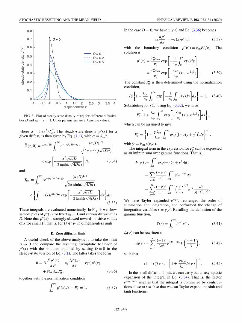
FIG. 3. Plot of steady-state density p∗(x) for different diffusivi-ties D and v0 = κ = 1. Other parameters are at baseline values.

where α = 3r0κ2/F 2

b . The steady-state density p∗(x) for agiven drift v0 is then given by Eq. (3.13) with σ = k−1

on :

(x, 0) = exv0/2D∫ ∞

0e−(v0

2/4D+r0 )t (α/D)1/4√2π sinh(t

√4Dα)

× exp

[− x2√α/D

2 tanh(t√

4Dα)

]dt, (3.34)

and

Tres =∫ ∞

0te−(v0

2/4D+r0 )t (α/D)1/4√2π sinh(t

√4Dα)

×{∫ ∞

0r(x)exv0/2D exp

[− x2√α/D

2 tanh(t√

4Dα)

]dx

}dt .

(3.35)

These integrals are evaluated numerically. In Fig. 3 we showsample plots of p∗(x) for fixed v0 = 1 and various diffusivitiesD. Note that p∗(x) is strongly skewed towards positive valuesof x for small D, that is, for D � v0 in dimensionless units.

D. Zero diffusion limit

A useful check of the above analysis is to take the limitD → 0 and compare the resulting asymptotic behavior ofp∗(x) with the solution obtained by setting D = 0 in thesteady-state version of Eq. (3.1). The latter takes the form

0 = Dd2 p∗(x)

dx2− v0

d p∗(x)

dx− r(x)p∗(x)

+ δ(x)konP∗0 , (3.36)

together with the normalization condition∫ ∞

0p∗(x)dx + P∗

0 = 1. (3.37)

In the case D = 0, we have x � 0 and Eq. (3.36) becomes

v0d p∗

dx= −r(x)p∗(x), (3.38)

with the boundary condition p∗(0) = konP∗0 /v0. The

solution is

p∗(x) = P∗0 kon

v0exp

[− 1

v0

∫ x

0r(y)dy

]= P∗

0 kon

v0exp

[−koff

v0(x + κ2x3)

]. (3.39)

The constant P∗0 is then determined using the normalization

condition,

P∗0

{1 + kon

v0

∫ ∞

0exp

[− 1

v0

∫ x

0r(y)dy

]dx

}= 1. (3.40)

Substituting for r(x) using Eq. (3.32), we have

P∗0

{1 + kon

v0

∫ ∞

0exp

[−koff

v0(x + κ2x3)

]dx

},

which can be arranged to give

P∗0 =

{1 + γ kon

koff

∫ ∞

0exp

([−γ (y + y3)

]dy

}−1

,

with γ = koff/(v0κ ).The integral term in the expression for P∗

0 can be expressedas an infinite sum over gamma functions. That is,

I0(γ ) :=∫ ∞

0exp[−γ (y + y3)]dy

=∞∑

n=0

(−γ )n

n!

∫ ∞

0yne−γ y3

dy

=∞∑

n=0

(−γ )n

n!

∫ ∞

0

(t

γ

)n/3

e−t dt

3(γ t2)1/3.

We have Taylor expanded e−γ y, rearranged the order ofsummation and integration, and performed the change ofintegration variables t = γ y3. Recalling the definition of thegamma function,

�(z) =∫ ∞

0t z−1e−t , (3.41)

I0(γ ) can be rewritten as

I0(γ ) =∞∑

n=0

(−1)n

3n!γ (2n−1)/3�

(n + 1

3

), (3.42)

such that

P0 = P∗0 (γ ) :=

[1 + γ kon

koffI0(γ )

]−1

. (3.43)

In the small diffusion limit, we can carry out an asymptoticexpansion of the integral in Eq. (3.34). That is, the factore−v0

2/4Dt implies that the integral is dominated by contribu-tions close to t = 0 so that we can Taylor expand the sinh andtanh functions:

022134-7

PAUL C. BRESSLOFF PHYSICAL REVIEW E 102, 022134 (2020)

(x, 0) ≈ exv0/2D∫ ∞

0e−(v0

2/4D+koff )t (α/D)1/4√2π t

√4Dα

exp

{− x2√α/D

2[t√

4Dα − (t√

4Dα)3/3]

}dt

≈ exv0/2D∫ ∞

0e−(v0

2/4D+koff )t 1√4πDt

exp

{− x2

4Dt[1 − 4Dαt2/3]

}dt

≈ exv0/2D∫ ∞

0e−(v0

2/4D+koff +αx2/3)t 1√4πDt

exp

(− x2

4Dt

)dt

= exv0/2D∫ ∞

−∞eikx

{∫ ∞

0e−(v0

2/4D+koff +αx2/3)t e−Dk2t dt

}dk

2π

= exv0/2D∫ ∞

−∞

eikx

Dk2 + v02/4D + koff + αx2/3

dk

2π

= 1√v0

2 + 4D(koff + αx3/3)exp

⎡⎣v0x

2D− v0|x|

2D

√1 + 4D(koff + αx2/3)

v02

⎤⎦.

We have used contour integration to evaluate the final kintegral. Finally, Taylor expanding the square-root functionsto leading order shows that

(x, 0) ∼ 1

v0e−x(koff +αx2/3)/v0

for x > 0 and

(x, 0) ∼ 1

v0e−|x|v0/D

for x < 0. Hence, if x > 0, then we recover the x dependenceof p∗(x) given by Eq. (3.39) for D = 0. On the other hand, ifx < 0, then p∗(x) → 0 as D → 0. These results are consistentwith Fig. 3.

IV. MULTIPLE ADHESION BONDS ANDMEAN-FIELD THEORY

We now extend the mean-field approach of Ref. [13] inorder to reduce the CK equation (2.8) to an effective single-particle CK equation with constant drift v0. The force-balanceequation is then used to derive a self-consistency conditionrelating the mean traction force and v0.

A. Mean-field approximation (fast binding limit)

It is convenient to first consider the fast binding limitkon → ∞. Equation (2.8) for ρ(x, t ) = ρ(x, t, q)|q=(1,...,1) canthen be written in the more compact form

∂ρ(x, t )

∂t= −

N∑i=1

∂J (x, t )

∂xi−

N∑i=1

r(xi)ρ(x, t ),

+N∑

i=1

δ(xi )∫ ∞

−∞r(x′

i )ρ(x, t )|xi=x′idx′

i. (4.1)

The probability flux is

J (x, t ) = −DN∑

j=1

∂ρ(x, t )

∂xi+ v(x)ρ(x, t ). (4.2)

Consider a particular bond labeled k and integrate both sidesof Eq. (4.1) with respect to x j for all j �= k. Defining

ρk (x, t ) =⎡⎣ N∏

j=1

∫ ∞

−∞dx j

⎤⎦δ(xk − x)ρ(x, t ), (4.3)

and

Jk (x, t ) =⎡⎣ N∏

j=1

∫ ∞

−∞dx j

⎤⎦δ(xk − x)J (x, t ), (4.4)

we find that

∂ρk (x, t )

∂t= −∂Jk (x, t )

∂xk− r(x)ρk (x, t )

+ δ(xk )∫ ∞

−∞r(x′)ρk (x′, t )dx′. (4.5)

Unfortunately, Eq. (4.5) is not a closed single-particle CKequation, since Jk (x, t ) depends on the full probability densityρ(x, t ). That is, substituting Eq. (4.2) into (4.4) gives

Jk (x, t ) =⎡⎣ N∏

j=1

∫ ∞

−∞dx j

⎤⎦δ(xk − x)

×[−D

∂ρ(x, t )

∂xk+ v(x)ρ(x, t )

]= − D

∂ρk (x, t )

∂x

+⎡⎣ N∏

j=1

∫ ∞

−∞dx j

⎤⎦δ(xk − x)v(x)ρ(x, t ). (4.6)

The mean-field approximation is to assume that for large N ,the individual bonds are statistically independent so that wecan factorize the multibond density into the product of N

022134-8

STOCHASTIC RESETTING AND THE MEAN-FIELD … PHYSICAL REVIEW E 102, 022134 (2020)

single-bond densities:

ρ(x, t ) =N∏

j=1

p(x j, t ), (4.7)

with ∫ ∞

−∞p(x, t )dx = 1.

Substituting this approximation into Eqs. (4.3) and (4.6)yields ρk (x, t ) = p(x, t ) and

Jk (x, t ) = J (x, t ) = −D ∂ p(x,t )∂x + 〈v(t )〉p(x, t )

for all k = 1, . . . , N , where

〈v(t )〉 = 1

ξ

[F − κN

∫ ∞

−∞|x|p(x, t )dx

]. (4.8)

Equation (4.5) is now a closed equation of the form

∂ p(x, t )

∂t= D

∂2 p(x, t )

∂x2− 〈v(t )〉∂ p(x, t )

∂x− r(x)p(x, t )

+ δ(x)∫ ∞

−∞r(x′)ρ(x′, t )dx. (4.9)

B. Mean-field approximation (finite kon)

The above analysis can be extended to the case of a finitebinding rate. Again select a particular bond k and introducethe marginal densities

ρk,1(x, t )∑

q

δqk ,1

⎡⎣ N∏j=1

∫ ∞

−∞dx j

⎤⎦δ(xk − x)ρ(x, t, q),

(4.10a)

ρk,0(t )∑

q

δqk ,0

⎡⎣ N∏j=1

∫ ∞

−∞dx j

⎤⎦ρ(x, t, q), (4.10b)

and

Jk (x, t ) =∑

q

δqk ,1

⎡⎣ N∏j=1

∫ ∞

−∞dx j

⎤⎦δ(xk − x)Jk (x, t, q).

(4.10c)Summing the full CK equation (2.8) with respect to qi and

integrating with respect to xi for all i �= k gives the followingpair of equations:

∂ρk,1(x, t )

∂t= −∂Jk (x, t )

∂xk− r(x)ρk,1(x, t )

+ δ(x)konρk,0(t ),

∂ρk,0(t )

∂t= −konρk,0(t ) +

∫ ∞

−∞r(x′)ρk,1(x′, t )dx′.

Again, we do not have a closed single-bond equation becauseρk,1(x, t ), ρk,0(t ), and Jk (x, t ) all depend on the full probabil-ity density. In particular, from Eq. (2.9)

Jk (x, t ) =∑

q

δqk ,1

⎡⎣ N∏j=1

∫ ∞

−∞dx j

⎤⎦δ(xk − x)

×[−D

∂ρ(x, t, q)

∂xk+ v(x)ρ(x, t, q)

]

= − D∂ρk,1(x, t )

∂x

+∑

q

δqk ,1

⎡⎣ N∏j=1

∫ ∞

−∞dx j

⎤⎦δ(xk − x)v(x)ρ(x, t, q).

Then mean-field approximation now becomes

ρ(x, t, q) =N∏

j=1

[q j p(x j, t ) + (1 − qj )P0(t )

], (4.11)

with ∫ ∞

−∞p(x, t )dx + P0(t ) = 1.

Substituting into Eqs. (4.10)–(4.10c) and setting ρk,1(x.t ) =p(x, t ) and ρk,0(t ) = P0(t ), we obtain the closed single-bondCK equation

∂ p(x, t )

∂t= D

∂2 p(x, t )

∂x2− 〈v(t )〉∂ p(x, t )

∂x− r(x)p(x, t )

+ δ(x)konP0(t ), (4.12a)

dP0(t )

dt= −konP0(t ) +

∫ ∞

−∞r(x′)p(x′, t )dx′. (4.12b)

C. Steady-state traction force

Although the time-dependent mean-field equation (4.12)involves a time-dependent drift 〈v(t )〉, the steady-state equa-tions are identical to the corresponding single-bond processwith a constant drift v0, see (3.36). Imposing the normal-ization condition means that the time-independent version ofEq. (4.12b) is automatically satisfied. The steady-state densityp∗(x) for fixed v0 can thus be determined using the analysisof Sec. III. The drift v0 and external force F are then relatedaccording to Eq. (4.8):

F = F (v0) = ξv0 + N f (v0), (4.13)

where f (v0) is the traction force

f (v0) = κ

∫ ∞

−∞|x|p∗(x; v0)dx. (4.14)

The steady-state behavior of the model can now be in-vestigated by fixing either the external drive F or the sliderspeed v0. We choose the latter here, since it avoids havingto solve an implicit equation for v0 as a function of F . Ourmain goal is to determine how the traction force f per linkageis affected by diffusion. Dimensionless quantities are usedby setting koff = 1, v = 1, and Fb = 1. We also assume thatN is sufficiently large so that the mean-field approximationholds. (In Ref. [13], numerical simulations of the full systemestablished that the mean-field approximation can break downif N or ξ is too small, since the rupture of one bond can triggera rupture cascade, resulting in alternating periods of stick andslip. Consequently, the joint probability distribution cannotbe factorized into a product of single-bond distributions. Thisargument carries over when diffusion of the slider is included,since the rupturing of a bond results in a steplike change in theelastic force whose size depends on κ/ξ , whereas a Wienerprocess is continuous. We will ignore this complication here.)

022134-9

PAUL C. BRESSLOFF PHYSICAL REVIEW E 102, 022134 (2020)

9 10 0

0.1

0.2

0.3

0.4

0.5

0.6

0.7

0.8

kon = 1

kon = 5

kon = 10

mea

n tr

actio

n fo

rce

f

mean velocity v0

7 8 6 4 5 3 1 2 0

FIG. 4. Plot of the mean traction force f as a function of themean velocity v0 for different values of the binding rate kon. Otherparameters are at baseline values: κ = koff = Fb = 1.

Within the specific context of FA dynamics, reference valuesfor various parameters are as follows [13]: koff = 1 s−1, v =10 nm s−1, Fb = 2 pN, and κ = 1 − 100 pN nm−1. Estimatesof the diffusivity D or the friction coefficient ξ are difficultdue to the complicated medium within which the stress fibersmove, which includes multiple interactions with the actincytoskeleton. Therefore, we will consider a range of valuesfor D.

The steady-state traction force f for D = 0 can be calcu-lated using Eqs. (3.39) and (4.14):

f = κ

∫ ∞

0xp∗(x)dx

= κP∗0 kon

v0

∫ ∞

0x exp

[− 1

v0

∫ x

0r(x′)dx′

]dx

= P∗0 kon

v0κ

∫ ∞

0y exp[−γ (y + y3)]dy.

Evaluating the integral along identical lines to I0(y), seeSec. III D, yields

I1(γ ) :=∫ ∞

0y exp[−γ (y + y3)]dy

=∞∑

n=0

(−1)n

n!γ (2n−2)/3�

(n + 2

3

), (4.15)

and

f = P∗0 (γ )kon

v0κI1(γ ). (4.16)

In Fig. 4 we sketch some example curves of the mean-fieldmodel, showing how the mean traction force f varies with thespeed v0. It can be seen from Fig. 4 that there is a maximumin the mean traction force at intermediate velocities. Thisis consistent with previous results in Ref. [13], and can beunderstood within the mean-field framework by noting thatthe average transmitted force of an engaged clutch increasesmonotonically with speed, while the probability of the clutch

0.02

0.04

0.06

0.08

0. 1

0.12

0.14

0.16

0.18

9 10

mea

n tr

actio

n fo

rce

f

spring constant κ7 864 531 20

v0 = 0.5v0 = 1v0 = 2

FIG. 5. Plot of the traction force f against the spring constant κ

for different speeds v0. Other parameters are at baseline values.

being bound decreases at higher speeds. Under the mean-fieldapproximation, the speed at maximum traction force is inde-pendent of the number of bonds and the friction coefficient ξ .In Fig. 5 we show analogous plots of f as a function of thespring constant κ , which acts as a proxy for stiffness of theECM.

The steady-state traction force f for D > 0 is given by

f = κ

∫ ∞

−∞|x|p∗(x)dx = κ

σ + Tres

∫ ∞

−∞|x|(x, 0)dx.

Substituting for (x, 0) and Tres using Eqs. (3.34) and (3.35),respectively, and evaluating the resulting integrals then yieldsf as a function of v0. In Figs. 6 and Fig. 7 we plot thetraction force f as a function of the mean velocity v0 andthe spring constant κ , respectively, for various values of thediffusivity D. It can be checked that in both cases the curvesconverge in the limit D → 0. We see that diffusion has the

9 10

mea

n tr

actio

n fo

rce

f

7 864 531 20

D = 0.1D = 1D = 5

mean velocity v0

0.04

0.06

0.08

0.1

0.12

0.14

0.16

0.18

D = 0

FIG. 6. Plot of steady-state traction force f as a function of themean speed v0 for various diffusivities D and κ = kon = 1.

022134-10

STOCHASTIC RESETTING AND THE MEAN-FIELD … PHYSICAL REVIEW E 102, 022134 (2020)

9 10

mea

n tr

actio

n fo

rce

f

spring constant κ7 864 531 20

D = 0.01D = 0.1D = 1D = 5

0.02

0.04

0.06

0.08

0. 1

0.12

0.14

0.16

0.18

FIG. 7. Plot of steady-state traction force f as a function ofthe effective spring constant κ for various diffusivities D and v0 =kon = 1.

effect of flattening the biphasic f − v0 curves. On the otherhand, diffusion sharpens the response with respect to κ byraising f for small κ and lowering f for large κ . In terms ofthe specific application to single FA dynamics, the sensitivityof the f − κ curves to diffusion suggests that fluctuations inthe driving force could play a role in the mechanosensing ofECM stiffness, as suggested in Ref. [21].

V. DISCUSSION

In this paper we used a mean-field approximation to reducea stochastic model of sliding friction to an effective single-bond model. We then mapped the latter to an equivalent modeldescribing an overdamped Brownian particle with spatiallydependent stochastic resetting and a refractory period. Thisallowed us to apply recent analytical methods developed forsystems with stochastic resetting, such as renewal theory andpath integrals, in order to investigate the effects of diffusionon the mean traction force per bond as a function of the springconstant. In particular, we found that diffusion can sharpenthe response. In terms of the application to FA dynamics, thissuggests that fluctuations in the driving force could enhancethe ability of the FA to act as a mechanosensor of ECM stiff-ness. However, a number of strong assumptions were madein the simplified model of sliding friction. First, the numberN of adhesion bonds was assumed to be sufficiently large sothat the mean-field approximation holds; as noted in Ref. [13],this assumption could break down in low friction regimesdue to rupture cascades. Second, both positive and negativedisplacements of a bond were modeled in terms of the linearextension of a Hookean spring. Thus adhesive linkages weretreated as slip rather than catch bonds, and geometric factorsarising from the conversion of linear displacements of theslider to bond extensions were ignored. Finally, the springconstant κ of each bond was treated as a lumped parameterthat included the stiffness of the ECM. A more detailed modelwould need to model the set of bound adhesive links in serieswith an ECM spring along the lines of Ref. [12].

One possible extension of the current work would beto consider other examples of collective cell adhesion. Forexample, cadherin-based cell-to-cell adhesions play a primaryrole in determining tissue structure. In addition to resistingexternal mechanical loads, recent evidence suggests that cad-herins also couple together the actomyosin cytoskeletons ofneighboring cells [37]. Hence, they are well placed to act aspowerful regulators of the cytoskeleton, and to activate diversesignaling pathways in response to applied load. At the cellularlevel, fluctuations in the number of engaged cadherin-basedlinkages are coupled to the assembly and disassembly of theactomyosin cytoskeleton of connected cells. This could pro-vide a force-dependent mechanism for consolidating certaintissue structures while supporting cellular rearrangements inother contexts. Again the stochastic breaking of a cadherin-based adhesion and subsequent rebinding could be modeledin terms of stochastic resetting with a refractory period.However, rather than modeling sliding friction, one couldnow investigate when a critical number of bonds are formedor broken by formulating the latter as a first passage timeproblem.

Finally, from a more general modeling perspective, ourpaper provides a concrete application of the theory of dy-namical processes with stochastic resetting to cell biology. Anumber of other recent examples include Michaelis-Mentenreaction schemes [38,39], DNA elongation and backtracking[40], and active cellular transport [41,42]. In each of thesecases, analytical tools such as renewal theory can be used toinvestigate the behavior of the system.

APPENDIX: Eigenfunction expansion of the propgator.

An alternative approach to evaluating (x, t ) is to con-sider an eigenfunction expansion of the propagator. Supposethat �r(x) acts like a confining potential [�r(x) → ∞ forx → ±∞], so there exists a complete set of orthonormaleigenfunctions φn(x), n = 0, 1, . . . , with[

−D∂2

∂x2+ �r(x)

]φn(x) = Enφn(x) (A1)

such that ∫ ∞

−∞φn(x)φm(x)dx = δn,m.

Then

Gr (x,−it |x0, 0) =∑n�0

e−Entφn(x0)φn(x). (A2)

If we now substitute the eigenfunction expansion (A2) intoEq. (3.30) and take the Laplace transform, we obtain the seriesexpansion

(x, s) = exv0/2D∑n�0

φn(0)φn(x)

s + r0 + v20/4D + En

. (A3)

Substituting into Eq. (3.13) gives

p∗(x) = exv0/2D lims→0

s∑

n�0φn(0)φn (x)

s+r0+v20/4D+En

1 − ψ (s)∑

n�0�nφn(0)

s+r0+v20/4D+En

,

022134-11

PAUL C. BRESSLOFF PHYSICAL REVIEW E 102, 022134 (2020)

where

�n =∫ ∞

0�r(y)eyv0/2Dφn(y)dy. (A4)

Applying L’Hopital’s rule and the normalization F (0) = 1yields the result

p∗(x) =exv0/2D

∑n�0

φn(0)φn(x)v2

0/4D+r0+En

1 + σ + ∑n�0

�nφn(0)(v2

0/4D+r0+En )2

. (A5)

Equation (A5) yields an explicit series expansion of thesteady-state density p∗(x). However, this is predicated onknowing the eigenfunctions and eigenvalues of the Hamilto-nian operator H . Again, there are only a few potentials forwhich exact results are known. In the particular case of a

harmonic potential, �r(x) = αx2, the eigenvalues are

En =(

n + 1

2

)√4Dα, (A6)

and the normalized eigenfunctions are

φn(x) = 1√2nn!

√π

(√α

D

)1/4

Hn[(α/D)1/4x]e−√α/Dx2/2,

(A7)

with Hn(x) the Hermite polynomial of integer order n. How-ever, it is simpler to use the explicit expressions given byEqs. (3.30) and (3.33). Although the eigenvalue problem forthe nonanalytic, symmetrized exponential potential r0eκ|x|/Fb

has also been analyzed [43], the numerical evaluation of theeigenvalues is rather delicate and not useful for our purposes.(The eigenfunctions are given by modified Bessel functionsKν and the eigenvalues are determined from the equationK

2i√

En/D(κ/Fb)2 [2√

r0/D(κ/Fb)2)] = 0.)

[1] J. T. Parsons, A. R. Horwitz, and M. A. Schwartz, Cell ad-hesion: Integrating cytoskeletal dynamics and cellular tension,Nat. Rev. Mol. Cell Biol. 11, 633 (2010).

[2] U. S. Schwarz and S. A. Safran, Physics of adherent cells, Rev.Mod. Phys. 85, 1327 (2013).

[3] M. Vicente-Manzanares, C. K. Choi, and A. R. Horwitz, Inte-grins in cell migration–the actin connection, J. Cell Sci. 122,199 (2009).

[4] T. J. Mitchison and M. W. Kirschner, Cytoskeletal dynamicsand nerve growth, Neuron 1, 761 (1988).

[5] C. H. Lin and P. Forscher, Growth cone advance is inverselyproportional to retrograde f-actin flow, Neuron 14, 763 (1995).

[6] C. Jurado, J. R. Haserick, and J. Lee, Slipping or gripping?Fluorescent speckle microscopy in fish keratocytes reveals twodifferent mechanisms for generating a retrograde flow of actin,Mol. Biol. Cell 16, 507 (2005).

[7] W. H. Guo and Y. L. Wang, Retrograde fluxes of focal adhesionproteins in response to cell migration and mechanical signals,Mol. Biol. Cell 18, 4519 (2007).

[8] G. Giannone, R. M. Mege, and O. Thoumine, Multi-levelmolecular clutches in motile cell processes, Trends Cell Biol.19, 475 (2009).

[9] A. Schallamach, A theory of dynamic rubber friction, Wear 6,375 (1963).

[10] A. E. Filippov, J. Klafter J, and M. Urbakh, Friction ThroughDynamical Formation and Rupture of Molecular Bonds, Phys.Rev. Lett. 92, 135503 (2004).

[11] M. Srinivasan and S. Walcott, Binding site models for frictiondue to the formation and rupture of bonds: State-functionformalism, force-velocity relations, response to slip veloc-ity transients, and slip stability, Phys. Rev. E 80, 046124(2009).

[12] C. E. Chan and D. J. Odde, Traction dynamics of filopodia oncompliant substrates, Science 322, 1687 (2008).

[13] B. Sabass and U. S. Schwarz, Modeling cytoskeletal flow overadhesion sites: Competition between stochastic bond dynam-ics and intracellular relaxation, J. Phys. Condens. Matter. 22,194112 (2010).

[14] Y. Li, P. Bhimalapuram, and A. R. Dinner, Model for howretrograde actin flow regulates adhesion traction stresses,J. Phys. Condens. Matter. 22, 194113 (2010).

[15] P. Sens, Rigidity sensing by stochastic sliding friction,Europhys. Lett. 104, 38003 (2013).

[16] B. L. Bangasser, S. S. Rosenfeld, and D. J. Odde, Determinantsof maximal force transmission in a motor-clutch model of celltraction in a compliant microenvironment, Biophys. J. 105, 581(2013).

[17] P. S. De and R. De, Stick-slip dynamics of migratingcells on viscoelastic substrates, Phys. Rev. E 100, 012409(2019).

[18] B. Ladoux and A. Nicolas, Physically based principles of celladhesion mechanosensitivity in tissues, Rep. Prog. Phys. 75,116601 (2012).

[19] J. Z Kechagia, J. Ivaska, and P. Roca-Cusachs, Integrins asbiomechanical sensors of the microenvironment, Nature Rev.Mol. Cel. Biol. 20, 457 (2019).

[20] C. M. Lo, H. B. Wang, M. Dembo, and Y. L. Wang, Cellmovement is guided by the rigidity of the substrate, Biophys.J. 79, 144 (2000).

[21] S. V. Plotnikov and C. M. Waterman, Guiding cell migration bytugging, Curr. Opin. Cell Biol. 25, 619 (2013).

[22] R. Sunyer and X. Trepat, Durotaxis, Curr. Biol. 30, R383(2020).

[23] S. V. Plotnikov, A. M. Pasapera, B. Sabass, and C. M.Waterman, Force fluctuations within focal adhesions mediateECM- rigidity sensing to guide directed cell migration, Cell151, 1513 (2012).

[24] M. R. Evans and S. N. Majumdar, Diffusion with StochasticResetting, Phys. Rev. Lett. 106, 160601 (2011).

[25] M. R. Evans and S. N. Majumdar, Diffusion with optimalresetting, J. Phys. A Math. Theor. 44, 435001 (2011).

[26] M. R. Evans and S. N. Majumdar, Diffusion with resetting inarbitrary spatial dimension, J. Phys. A: Math. Theor. 47, 285001(2014).

[27] M. R. Evans, S. N. Majumdar, and G. Schehr, Stochasticresetting and applications, J. Phys. A 53, 193001 (2020).

022134-12

STOCHASTIC RESETTING AND THE MEAN-FIELD … PHYSICAL REVIEW E 102, 022134 (2020)

[28] A. Pal, Diffusion in a potential landscape with stochastic reset-ting, Phys. Rev. E 91, 012113 (2015).

[29] E. Roldan and S. Gupta, Path-integral formalism for stochasticresetting: Exactly solved examples and shortcuts to confine-ment, Phys. Rev. E 96, 022130 (2017).

[30] M. R. Evans and S. N. Majumdar, Effects of refractory periodon stochastic resetting, J. Phys. A: Math. Theor. 52, 01LT01(2019).

[31] G. I. Bell, Models for specific adhesion of cells to cells, Science200, 618 (1978).

[32] E. Evans and K. Ritchie, Dynamic strength of molecular adhe-sion bonds, Biophys. J. 72, 1541 (1997).

[33] P. C. Bressloff, Stochastic Processes in Cell biology (Springer,New York, 2014).

[34] More precisely, in the analysis of Ref. [13] the displacementsare restricted to be positive, xi � 0 for all i = 1, . . . , N . Theterm Ai(x, , t, q) multiplying δ(xi ) in Eq. (2.8) is modifiedaccordingly:

Ai = (1 − qi )∫ ∞

0r(x′

i )ρ(x, t, q)|(xi,qi )=(x′i ,1)dx′

i

+ qi[konρ(x, t, q)|qi=0 − J (x, t, q),

with flux J (x, t, q) = v(x)ρ(x, t, q). The inclusion of the fluxterm ensures conservation of flux at each boundary x j = 0.

[35] R. P. Feynman and A. R. Hibbs, Quantum Mechanics and PathIntegrals (McGraw–Hill, New York, 2010).

[36] L. S. Schulman, Techniques and Applications of Path Integration(John Wiley Sons, Chichester, UK, 1981).

[37] B. D. Hoffman and A. S. Yap, Towards a dynamic understand-ing of cadherin-based mechanobiology, Trends Cell Biol. 25,803 (2015).

[38] S. Reuveni, M. Urbakh, and J. Klafter, Role of substrate unbind-ing in Michaelis-Menten enzymatic reactions, Proc. Natl Acad.Sci. USA 111, 4391 (2014).

[39] T. Rothart, S. Reuveni, and M. Urbakh, Michaelis-Mentenreaction scheme as a unified approach towards theoptimal restart problem, Phys. Rev. E 92, 060101(2015).

[40] E. Roldan, A. Lisica, D. Sanchez-Taltavull, and S. W. Grill,Stochastic resetting in backtrack recovery by RNA poly-merases, Phys. Rev. E 93, 062411 (2016).

[41] P. C. Bressloff, Directed intermittent search with stochasticresetting, J. Phys. A 53, 105001 (2020).

[42] P. C. Bressloff, Modeling active cellular transport as a directedsearch process with stochastic resetting and delays, J. Phys. A53, 355001 (2020).

[43] M. Znojil, Symmetrized exponential oscillator, Mod. Phys. Lett.A 31, 1650195 (2016).

022134-13