PHYSICAL REVIEW A 100, 032111 (2019)

Macroscopicity of quantum mechanical superposition tests via hypothesis falsification

Björn Schrinski,1 Stefan Nimmrichter,2 Benjamin A. Stickler,1,3 and Klaus Hornberger 1

1University of Duisburg-Essen, Faculty of Physics, Lotharstraße 1, 47048 Duisburg, Germany2Max Planck Institute for the Science of Light, Staudtstraße 2, 91058 Erlangen, Germany

3QOLS, Blackett Laboratory, Imperial College London, London SW7 2BW, United Kingdom

(Received 28 February 2019; published 16 September 2019)

We establish an objective scheme to determine the macroscopicity of quantum superposition tests withmechanical degrees of freedom. It is based on the Bayesian hypothesis falsification of a class of macrorealistmodifications of quantum theory, such as the model of continuous spontaneous localization. The measure usesthe raw data gathered in an experiment, taking into account all measurement uncertainties, and can be used todirectly assess any conceivable quantum mechanical test. We determine the resulting macroscopicity for threerecent tests of quantum physics: double-well interference of Bose-Einstein condensates, Leggett-Garg tests withatomic random walks, and entanglement generation and read-out of nanomechanical oscillators.

DOI: 10.1103/PhysRevA.100.032111

I. INTRODUCTION

Any experiment witnessing or exploiting quantum coher-ent phenomena may be viewed as a test of whether quantumtheory is complete at a fundamental level. While quantummechanics is supported by all empirical observations up todate, all these observations are equally compatible with anumber of alternative theories restoring macroscopic realismand resolving the measurement problem [1,2].

In recent years, various experiments demonstrated quan-tum superpositions or entanglement with mechanical objectsof increasingly high masses and particle number, involvingever larger spatial delocalizations and coherence times. Theyinclude setups as diverse as counterpropagating superconduct-ing loop currents [3,4], large path-separation atom interfer-ometers [5,6], high-mass molecular near-field interferometers[7,8], trapped and freely falling Bose-Einstein condensates[9,10], delocalized states and Leggett-Garg tests in optical lat-tices [11,12], entangled ion chains [13,14], and nanomechan-ical oscillators [15–17]. While all these experiments establishvariants of a Schrödinger-cat-like state, an obvious question isthe degree of macroscopicity reached.

There are many ways to assess the macroscopicity of aSchrödinger cat state realized in a quantum experiment [18].Most measures quantify the complexity of the quantum statebased on information- or resource-theoretic concepts [19–23],or introduce suitable distance measures in Hilbert space[24,25]. While such abstract state vector ranking schemesmay be used to compare experimental setups of similar kind,none can cover the entire variety of present-day superpositionexperiments [3–17].

A viable alternative is to regard a Schrödinger cat state asmore macroscopic than others if its demonstration is more atodds with the classical expectations shaped by our every-dayexperiences. In Ref. [26] this was cast into a macroscopicitymeasure by quantifying the extent to which a superpositionexperiment rules out a natural class of objective modifica-tions of quantum theory that predict classical behavior onthe macroscale. A prominent example of such classicaliz-

ing modifications is the model of continuous spontaneouslocalization (CSL) [2]. Recent tests of nonlocality and macro-realism, demonstrating the violation of Bell and Leggett-Garginequalities at unprecedented mass and timescales, call for ageneralization of this measure for arbitrary quantum tests withmechanical degrees of freedom.

In this article we present the most general framework forassigning the macroscopicity reached in quantum mechanicalsuperposition experiments, based on noninformative Bayesianhypothesis testing, see Fig. 1. As the natural generalization ofthe measure presented in [26], it relies only on the empiricalevidence (i.e., the raw measurement outcomes) delivered by agiven superposition test. It thus accounts for the measurementimperfections independently of the chosen experimental fig-ure of merit, such as the fringe visibility or an entanglementwitness.

This measure of macroscopicity can be applied to assessany mechanical superposition experiment. It is unbiased byconstruction and it accounts naturally for experimental uncer-tainties and statistical fluctuations. These advantages come atthe expense of a certain theoretical effort required for calculat-ing the macroscopicity of a given experiment. Specifically, thetime evolution of the quantum system must be calculated inthe presence of classicalizing modifications to obtain the prob-ability distribution for all possible measurement outcomes. Inthe second part of this article we demonstrate how this taskis accomplished for three superposition tests at the cuttingedge of quantum physics: double-well interference of number-squeezed Bose-Einstein condensates (BECs) [9], Leggett-Garg inequality tests with atomic quantum random walks [12],and generation and witnessing of entanglement between twospatially separated nanomechanical oscillators [15].

II. MACROSCOPICITY OF THREE RECENTSUPERPOSITION TESTS

Before presenting the formal framework of the proposedmeasure of macroscopicity, we illustrate its application tothree recent superposition tests [9,12,15]. As a common

2469-9926/2019/100(3)/032111(18) 032111-1 ©2019 American Physical Society

BJÖRN SCHRINSKI et al. PHYSICAL REVIEW A 100, 032111 (2019)

FIG. 1. Scheme to compare the macroscopicity of two differentquantum superposition tests: The experiments deliver raw data setsd1 and d2, which may be of arbitrary type and structure. They canbe used to rule out modifications of standard quantum theory whichclassicalize the dynamics. Combining the data with the theoreticalexpectation yields a probability distribution for the classicalizationtimescale τe, given the modification parameters σ and the back-ground information I . A quantum experiment is considered moremacroscopic if the data rule out greater values of τe, as inferred fromthe 5% quantile τm.

theme, these experiments use derived quantities, such asvisibilities, correlation functions, and entanglement witnesses,to certify the quantumness of their observations. One impor-tant advantage of the Bayesian approach advocated here isthat it is independent of such data processing (and thus ofsecondary observables) and based exclusively on likelihoodsassociated with elementary measurement events. A theoreticalderivation of the likelihoods required to assess the threementioned experiments is presented in Secs. IV–VI.

The measure uses the experimental data d to determinethe posterior probability distribution p(τe|d, σ, I ) ofclassicalization timescales τe, given the modificationparameters σ , and any background information I requiredto model the experiment. To ensure that each experimentis rated without bias, the least informative prior is used forBayesian updating to yield the final posterior distribution.Figures 2–4 show how disparate experimental measurementprotocols and data sets [9,12,15] yield comparable posteriordistributions, narrowly peaked around a definite modificationtimescale. As an increasing number of data points is includedin the Bayesian updating procedure, the distributions shift tohigher modification timescales, while their widths decrease.The lowest 5% quantile τm(σ ) of the posterior distributiondetermines the macroscopicity as

μm = maxσ

[log10

(τm(σ )

1 s

)].

The value μm thus quantifies the degree to which the quantummeasurement data rules out a natural class of classicalizingmodifications of quantum theory.

The resulting macroscopicities of the experiments are:μm = 8.5 for the BEC interferometer [9], μm = 7.1 forthe atomic Leggett-Garg test [12], and μm = 7.8 for theentangled nanobeams. That the BEC and the atomic randomwalk experiments exhibit comparable macroscopicities is dueto the fact that they both witness single atom interferenceat a similar product of squared mass and coherence time.The macroscopicity associated with the entangled nanobeamexperiment is roughly on the same order of magnitude onthe logarithmic scale, despite the high mass and the largeseparation between the two beams and as well as coherencetimes of microseconds. This surprising result can be explainedby the fact that the probed superposition state is delocalizedmerely by a few femtometers, and thus probes quantumtheory only on subatomic scales.

Comparison of the three experiments also reveals thatthe convergence rate of the posterior distribution can varystrongly. In case of the Leggett-Garg test with an atomicquantum random walk [12], the data set consists of 627 walkswhich all end in one of five final lattice sites. Since the likeli-hood of two of those outcomes is independent of the modifica-tion they include no information for the hypothesis test, whichslows the convergence of the Bayesian updating procedure. Incontrast, the double-well BEC interferometer [9] provides adistribution of measurement outcomes over a practically con-tinuous range of values, so that each experimental run yields ahigh degree of information gain, implying that 1457 measuredpopulation imbalances lead to a relatively narrow posteriordistribution. In the case of nanobeams only two of fourpossible coincidence outcomes have different likelihoods,and thus several thousand repetitions of the measurementprotocol are required to make the posterior converge.

III. MACROSCOPICITY VIA HYPOTHESISFALSIFICATION

A. Empirical measure of macroscopicity

Classicalizing modifications of quantum theory proposean alternative (stochastic) evolution equation for the wavefunction. The observable consequences of these alternativetheories are then encoded in the dynamics of the stateoperator ρt , which evolves according to a modified vonNeumann equation

∂tρt = Lρt + 1

τeMσ ρt . (1)

Here Lρt denotes the time evolution according to standardquantum theory (including possible decoherence) andMσ ρt/τe describes the effect of the proposed modification,characterized by the timescale τe and the set of modificationparameters σ .

Indeed, a generic class of modification theories are compat-ible with all observations up to date, and they restore realismon the macroscale. This class can be parametrized by impos-ing a few natural consistency requirements, such as Galileaninvariance and exchange symmetry [26]. The parameters σ =(σq, σs) with the dimensions of momentum and length, respec-tively, then specify the length and momentum scale on which

032111-2

MACROSCOPICITY OF QUANTUM MECHANICAL … PHYSICAL REVIEW A 100, 032111 (2019)

FIG. 2. (a) Schematic illustration of the double-well BEC interference experiment [9]. The BEC is initially split into a superpositionbetween slightly detuned left and right double-well states, then number squeezed, then let to freely evolve for a delay time, before a finalπ/2-pulse (recombiner) converts the phase difference between the states into an occupation difference. (b) Time-of-flight measurement dataof the occupation imbalance versus delay time (from Ref. [9]). (c) Posterior distribution of the classicalization timescale (red solid line) asobtained via Bayesian updating of Jeffreys’ prior (black dashed line) with the measurement data. The blue line is the intermediate distributionobtained by using only the blue data points up to 1 ms in (b). The shaded areas indicate the lowest 5% quantiles and all distributions arenormalized to the same maximum value.

-2 -1 0 1 2

FIG. 3. (a) Schematic illustration of the quantum random walk consisting of four consecutive steps. In each step the atom is coherentlysplit into a left- and right-moving state, and the final populations are read-out after the fourth step. (b) Experimental data from Ref. [12]. Theblue solid line is the data from the total quantum random walk, while the red lines are conditioned on the first step being either left (dashed)or right (dotted). (c) Posterior distribution of the classicalization timescale (red solid line) as obtained via Bayesian updating of Jeffreys’ prior(black dashed line) with the measurement data. The blue line is the intermediate distribution obtained by using only the blue measurement runsin (b). The shaded areas indicate the lowest 5% quantiles and all distributions are normalized to the same maximum value.

+

-107 1080.0

0.2

0.4

0.6

0.8

1.0

FIG. 4. (a) Stoke’s scattering of a pump photon, prepared in a spatial superposition by the entrance beam splitter, generates entanglementbetween two nanomechanical oscillators, which is then read-out by anti-Stoke’s scattering of a read photon. Entanglement is certified by acoincidence measurement of the scattered photons in the upper (+) or lower (−) detector behind the exit beam splitter. (b) Measurementdata [15] as a function of the tunable relative phase θ between the two interferometer arms (phase sweep). (c) Posterior distribution of theclassicalization timescale (red solid line) as obtained via Bayesian updating of Jeffreys’ prior (black dashed line) with the measurement data.The blue line is the posterior obtained by taking only phase sweep data points into account, while the red line also accounts for measurementswith variable time delay between pump and read [time sweep; not shown in (b)]. The shaded areas indicate the lowest 5% quantiles and alldistributions are normalized to the same maximum value.

032111-3

BJÖRN SCHRINSKI et al. PHYSICAL REVIEW A 100, 032111 (2019)

the modification acts by means of the distribution functiongσ (q, s) with zero mean and widths σq, σs,

Mσ ρt =∫

d3qd3s gσ (q, s)

[L(q, s)ρt L†(q, s)

− 1

2

{L†(q, s)L(q, s), ρt

}]. (2)

The Lindblad operators in second quantization,

L(q, s) =∑

α

mα

me

∫d3p eip·mes/mα hc†

α (p)cα (p − q) , (3)

induce displacements in phase space by means of the annihila-tion operator cα (p) for momentum p. They involve a sum overthe different particle species α with mass mα , whose ratio overthe electron mass me effectively amplifies the strength of themodification for heavy particles, ensuring that macrorealismis restored [26].

Roughly speaking, phase-space superpositions of a particleof mass mα will decohere at the maximal amplified rate(mα/me)2/τe if they extend over spatial distances greater thanh/σq or momentum distances greater than mα h/meσs. Wetake gσ to be Gaussian in the following. The modification(2) then reduces to the model of CSL [2] for fixed σq andσs = 0. As explained in Ref. [26], the bounds h/σq � 10 fmand σs � 20 pm ensure that the modification does not drivethe system into the regime of relativistic quantum mechanics.In what follows, we will define the empirical measure ofmacroscopicity as the extent to which a quantum experimentrules out such classicalizing modifications.

Since the modified evolution (1) predicts deviations fromstandard quantum mechanics at some scale these modifica-tion theories are empirically falsifiable. Thus, any quantumexperiment gathering measurement data d can be consideredas testing the hypothesis Hτ ∗

e:

Given a classicalizing modification (2) with parameters σ , thedynamics of the system state ρt are determined by Eq. (1) witha modification timescale τe � τ ∗

e .

Note that greater values of τe imply weaker modifications.The empirical data d determine the Bayesian probability

P(Hτ ∗e|d, σ, I ) that Hτ ∗

eis true, given the background informa-

tion I . The latter includes all knowledge required for describ-ing the experiment, such as the Hamiltonian, environmentaldecoherence processes, and the measurement protocol.

In order to compare Hτ ∗e

with the complementary hypoth-esis H τ ∗

ethat the modification time scale τe is larger than τ ∗

e(including unmodified quantum mechanics as τe = ∞), onedefines the odds ratio [27]

o(τ ∗e |d, σ, I ) = P

(Hτ ∗

e

∣∣d, σ, I)

P(H τ ∗

e

∣∣d, σ, I) . (4)

If the data implies that the odds ratio is less than a certainmaximally acceptable value om we can favor H τ ∗

eover Hτ ∗

e.

Modifications of quantum theory with τe � τ ∗e are then ruled

out by the data at odds om.In order to evaluate the odds ratio (4) we use Bayes’

theorem and exploit that for the hypothesis test to be unbiasedby earlier experiments, Hτ ∗

eand H τ ∗

emust be a priori equally

probable. Further using that the hypothesis Hτ ∗e

implies τe �

τ ∗e yields

o(τ ∗e |d, σ, I ) =

∫ τ ∗e

0 dτe P(d|τe, σ, I )p(τe|σ, I )∫∞τ ∗

edτe P(d|τe, σ, I )p(τe|σ, I )

, (5)

where p(τe|σ, I ) is the prior distribution of τe, whose choicewill be discussed in Sec. III B. The probabilities P(d|τe, σ, I )are independent of the hypothesis Hτ ∗

e; they can be calculated

for any experiment by solving the modified evolution equation(1) with classicalization timescale τe and parameters σ .

The data d is usually gathered in N consecutive indepen-dent runs, d = {d1, d2, . . . , dN }, where dk denotes the set of(possibly correlated) measurement outcomes of round k. Thelikelihood for the entire data set d is then given by

P(d|τe, σ, I ) =∏

k

P(dk|τe, σ, I ). (6)

Every additional experimental run thus refines the posteriorprobability density, according to Bayes’ theorem

p(τe|d, σ, I ) = P(d|τe, σ, I )p(τe|σ, I )

P(d|σ, I ), (7)

where the normalization constant P(d|σ, I ) plays no rolefor the odds ratio. For sufficiently large data sets and forwell behaved priors the posterior is independent of the priordistribution p(τe|σ, I ) [28,29].

For what follows, we choose the threshold odds om = 1 :19, corresponding to the posterior probability

P(τe � τm|d, σ, I ) ≡∫ τm

0dτe p(τe|d, σ, I ) = 5%. (8)

This determines the greatest excluded modification timescaleτm (at odds om) so that for all τ ∗

e � τm the odds ratio (5) issmaller than om for given modification parameters σ .

Given the greatest excluded modification timescale τm(σ )as a function of the modification parameters σ , one defines theempirical measure of macroscopicity as

μm = maxσ

[log10

(τm(σ )

1 s

)], (9)

where τm(σ ) [Eq. (8)] is the extent to which the measurementdata d of a given quantum experiment rules out the class ofmodifications (2). The value of μm thus ranks superpositionexperiments against each other according to the degree towhich they are at odds with our classical expectation.

We emphasize that this definition must only be used forexperiments that undeniably show genuine quantum signa-tures. It cannot be used to certify whether a given experimentobserves a superposition state. This is due to the fact thatthe absence of modification-induced heating and momentumdiffusion can be observed also in classical experiments. Eventhough quantum coherence plays no role in such setups,they can serve to exclude combinations of classicalizationtimescales and modification parameters [30–38].

Even in genuine quantum superposition experiments theobserved absence of modification-induced heating may dom-inate the range of excluded modification parameters. In thiscase it is necessary to recombine the observables in such away that they separate into a subset of random variables Dproviding information about quantum coherence and a subset

032111-4

MACROSCOPICITY OF QUANTUM MECHANICAL … PHYSICAL REVIEW A 100, 032111 (2019)

Dheat yielding only information about the energy gain. (Forexample, in the case of the double-well BEC interference ex-periment, where one measures the particle numbers in the twodifferent wells, their difference shows interference based onquantum coherence, while their sum constraints particle lossdue to heating.) For a fair assessment of the macroscopicity,the likelihood P(D, dheat|τe, σ, I ) must be conditioned on therealized data dheat restricting modification induced heating,

P(D|τe, σ, I, dheat ) = P(D, dheat|τe, σ, I )

P(dheat|τe, σ, I ), (10)

with P(dheat|τe, σ, I ) =∑D P(D, dheat|τe, σ, I ). This way thewitnessed lack of heating is effectively added to the back-ground information I . (It also shows how to formally takeinto account the observation that the experiment couldbe executed at all, i.e., that the setup did not disintegrate dueto modification-induced heating.) In Sec. IV we demonstratehow the conditioning on quantum observables works in prac-tice by means of a nontrivial example.

B. Jeffreys’ prior

If the data set is not sufficiently large, the measure (9)will in general depend on the prior distribution chosen toevaluate the odds ratio (5). It is therefore necessary to specifywhich prior distribution p(τe|σ, I ) must be used to calculatethe macroscopicity (9).

In order to ensure that the macroscopicity μm does not havea bias towards a selected class of quantum superposition tests,the prior must be chosen in the most uninformative way, i.e.,without including any a priori beliefs. For instance, this im-plies that it must not play a role whether we use the timescaleτe or the rate 1/τe to parametrize the class of modifications,which already excludes a uniform or piecewise-constant prior.Therefore, the natural choice is Jeffreys’ prior [39]. Given thelikelihood P(d|τe, σ, I ) associated with a random variable d ,it is defined as the square root of the Fisher information,

p(τe|σ, I ) ∝√I (τe|σ, I )

=√√√√⟨( ∂

∂τelog[P(D|τe, σ, I )]

)2⟩

D

. (11)

The ensemble average 〈·〉D is performed over the entirerange of possible measurement outcomes D with probabilityP(D|τe, σ, I ).

This prior coincides with the so-called reference prior, sothat it maximizes the Kullback-Leibler divergence betweenprior and posterior and thus the average information gainin the Bayesian updating process (7) [40,41]. In this sense,Jeffreys’ prior can be considered as the least informative prior[42]. In addition, it is invariant under reparametrizations of themodel [39], implying that it is irrelevant whether we use thetimescale τe or the rate λ = 1/τe (as employed in the model ofcontinuous spontaneous localization [2]) or any other powerof τe as the fundamental parameter of our model. We demon-strate in Appendix A that for all practical purposes Eq. (11)yields a normalizable posterior distribution (7) because themaster equation (1) and thus the likelihood P(d|τe, σ, I ) aresmooth functions of τe.

If different measurement protocols are implemented, in-dicated here by the index k (typical scenarios are differentwaiting times in a time integrated interferometer), Jeffreys’prior is weighted as

p(τe|σ, I ) ∝√∑

k

Nk I (τe|σ, Ik ). (12)

Here Nk is the number of experimental runs with the respectiveP(Dk|τe, σ, Ik ). The simple form of Jeffreys’ prior (12) canbe obtained by noting that 〈∂τe log[P(Dk|τe, σ, Ik )]〉Dk = 0 inany case since the normalization of the probability distributionP(Dk|τe, σ, Ik ) must be preserved for all τe.

C. General scheme for assigning macroscopicities

The formal framework of how to assess the macroscopicityof arbitrary quantum mechanical superposition tests is nowcomplete:

(1) Determine the Hamiltonian, environmental decoher-ence channels, and quantum measurement protocol, and usethese to calculate the likelihood P(D|τe, σ, I ) in the presenceof the modification (2). If appropriate use Eq. (10) to focus ondata demonstrating quantum coherence.

(2) Calculate Jeffreys’ prior (12).(3) Determine the posterior distribution via Bayesian up-

dating (7) to extract τm(σ ) via (8).(4) Find the maximum of the function τm(σ ), which deter-

mines the macroscopicity (9).This recipe prescribes how to calculate the macroscopicity

based on the empirical evidence of a quantum experiment. Itformalizes and generalizes the notion of macroscopicity in-troduced in Ref. [26]. The approximate expressions derived inRef. [26] intrinsically assume that imperfections of a given ex-periment yield a definite value of τe < ∞, corresponding to adelta-peaked posterior distribution. The Bayesian frameworkput forward here extends this to measurement schemes anddata sets yielding a finite posterior distribution p(τe|d, σ, I ).It is thus the natural extension for noisy data and arbitrarymeasurement strategies.

In practice, the most complicated part of the above schemeis calculating the likelihoods in step 1. This requires findingan appropriate and quantitative description of the quantum dy-namics in the presence of decoherence and the modification.Note that the macroscopicity is underestimated if relevantdecoherence channels are neglected in the calculation of thelikelihoods. The remainder of this article demonstrates howthe likelihoods can be calculated for the three superpositiontests discussed in Sec. II.

IV. RAMSEY INTERFEROMETRY WITH ANUMBER-SQUEEZED BEC

A. Experimental setting and basics

In the experiment reported in Ref. [9] a 87Rb BEC istrapped in a double-well potential and made to interfere, seeFig. 2(a). The two involved modes a, b form an effectivetwo-level system described by the annihilation operators ca,cb. The state of the BEC can thus be represented by a col-lective pseudospin, defined by means of the (dimensionless)

032111-5

BJÖRN SCHRINSKI et al. PHYSICAL REVIEW A 100, 032111 (2019)

-50 0 500

0.010.020.030.040.050.060.07

0

0

0 0

0

0 0

0

0

-50 0 500

0.010.020.030.040.050.060.07

-50 0 500

0.010.020.030.040.050.060.07

-50 0 500

0.010.020.030.040.050.060.07

FIG. 5. (a)–(c) The dynamics of large collective spin states close to the equator of a generalized Bloch sphere can be effectively describedby first evolving the state in the local tangent plane and then wrapping it back around the sphere. (d)–(f) Exact simulations of the BEC numberdifferences (red histograms) are in very good agreement with the analytical approximation (25) (black lines). The simulation was performedfor N = 100 particles and an initial variance of J2

z = N/5, reached by means of one-axis squeezing [44]. The snapshots are taken at times(d) t0 = 0, (e) t1 = 5.25π h/ε, and (f) t2 = 400π h/ε with �P = ζ = 0.002ε/h. At time t2 the distributions have practically converged towardsthe fully dephased steady state. (g) In the absence of phase diffusion the distribution exhibits (partial) revivals, as illustrated in (g) for time t2.[A complete revival to the state shown in (a) would first be observed at t = 1000π h/ε.]

quasiangular momentum operators [43]

Jx = 1

2(c†

acb + c†bca),

Jy = 1

2i(c†

acb − c†bca),

Jz = 1

2(c†

aca − c†bcb). (13)

They fulfill the angular momentum commutation relations[Jλ, Jμ] = iελ,μ,νJν . The simultaneous eigenstates of J2 witheigenvalue J (J + 1) and Jz with eigenvalue m are denoted by|J, m〉 (Dicke state), where J = N/2.

The product of N bosons being in a superposition state(coherent spin state, CSS) can be represented on a generalizedBloch sphere (see Fig. 5), whose polar angle θ indicates therelative population in a and b, while the azimuth φ is therelative phase of the superposition state. Such a product state|θ, φ〉 can be expanded in terms of Dicke states as

|θ, φ〉 ≡ 1√(2J )!

[cos

(θ

2

)c†

a + eiφ sin

(θ

2

)c†

b

]2J

|vac〉

=J∑

m=−J

(2J

J + m

)cos

(θ

2

)J−m

sin

(θ

2

)J+m

× e−i(J+m)φ |J, m〉. (14)

It has minimal and symmetric uncertainties, e.g., J2z =

J2y = |〈Jx〉/2| = J/2 for θ = π/2 and φ = 0.Applying a nonlinear squeezing operator turns the CSS

into a squeezed spin state (SSS) [44,45], which can be

useful for metrology [46–48] or robust against dephasingprocesses [9,49]. In addition, it has been demonstrated thatthe depth of entanglement increases with squeezing [50–52],as quantified by the squeezing parameter ξ 2 = 2(Jmin)2/J .We note that according to the information-theoretic measurefrom Ref. [21] already the existence of such a state yields alarge macroscopicity since squeezing increases the quantumFisher information.

In terms of the depth of entanglement [51,52] the non-classicality of SSS lies between a product state (CSS) andthe maximally entangled NOON state |ψ〉 ∝ |N, 0〉 + |0, N〉,a superposition of all particles being either in mode a ormode b. Applying the modification on this NOON stateyields a decoherence rate proportional to N2, while that ofa product state is proportional to N . It is thus easy to seethat a NOON state with stable phase could serve to excludea large range of classicalization timescales [53], but theyhave not been generated experimentally thus far. In contrast,the modification-induced dynamics of SSS, which are fre-quently realized in experiments, is much more intricate, asdiscussed in the following.

The free time evolution Lρ = −i[H, ρ]/h of the BEC ischaracterized by the energy difference ε between the twomodes and by the interaction between the particles. Approxi-mating the latter to leading order in Jz, yields the Hamiltonian[49]

H = εJz + hζJ2z , (15)

where ζ = dμ/d (hm)|m=0 is the change of chemical potentialwith the occupation difference m. Thus, the first term of theHamiltonian describes rotations around the z axis with angular

032111-6

MACROSCOPICITY OF QUANTUM MECHANICAL … PHYSICAL REVIEW A 100, 032111 (2019)

frequency ε/h on the generalized Bloch sphere, while thesecond term leads to dispersion.

The experiment starts with the BEC in the state |θ =π/2, φ = 0〉, which is then squeezed in z direction and freelyevolved for up to 20 ms. Finally, a π/2 rotation around the xaxis converts the phase distribution into mode occupation dif-ferences, which are read-out by time-of-flight measurements,see Fig. 2.

The likelihood required for the hypothesis test is the prob-ability of observing a number difference of m between the twomodes,

P(m|τe, σ, I ) =∞∑

J=0

〈J, m|e−iπJx/2ρt eiπJx/2|J, m〉,

=∞∑

J=0

P(J|τe, σ, I )PJ (m|τe, σ, I ) (16)

where the sum over J accounts for the possibility ofmodification-induced particle loss from the BEC during theexperiment [30]. The modification parameters τe and σ enterthrough the modified time evolution of the state ρt , which willbe discussed next.

B. Double-well potential: Phase flips

Expanding the momentum annihilation operators c(p) inEq. (3) in the single-particle eigenmodes in the presence of thepotential, and neglecting particle loss for the moment (c†

aca +c†

bcb = 2J), yields

Mσ ρ = 4m2Rb

τem2e

∫d3q fσ (q)

×[A(q)ρA†(q) − 1

2{A†(q)A(q), ρ}

]. (17)

Here we used that spatial displacements are negligible on thelength scale of the experiment and thus fσ (q) = ∫ dsgσ (q, s)depends only on σq. The Lindblad operators are given by

A(q) = ax(q)Jx + az(q)Jz , (18)

with

ax(q) = 〈ψa|W(q)|ψb〉,

az(q) = i〈ψa|W(q)|ψa〉 sin

(xqx

2h

)eixqx/2h. (19)

Here |ψa〉 and |ψb〉 are the single-atom eigenstates of thetwo level system with real wave functions ψb(r) = ψa(r −xex ) ∈ R and W(q) = exp(iq · r/h) is the momentum trans-fer operator.

The first part of the Lindblad operator describes rotationsaround the x axis, or spin flips, while the second one inducesrotations around the z axis, or phase flips. Such flip operatorsare frequently used to describe disturbance channels in col-lective spin states [45,54]. Since the spatial overlap betweenthe two modes is negligible, ax(q) az(q), the spin-flipcontribution will be neglected in the following, implying that〈J2

z 〉t remains constant.

The expectation value of the perpendicular spin compo-nents decays as 〈Jy〉t = e−�Pt/2〈Jy〉f,t with phase-flip rate (ordephasing rate)

�P = 4m2Rb

τem2e

∫d3q fσ (q)|az(q)|2. (20)

Here 〈Jy〉f,t denotes the free time evolution of the expectationvalue due to Eq. (15); the same relation holds for 〈Jx〉t . Notethat the phase-flip decay rate �P is independent of the degreeof squeezing.

The phase-flip operators induce diffusion in the azimuthalplane of the generalized Bloch sphere. The second moment ofJy thus evolves as

⟨J2

y

⟩t= 1

2

⟨J2

x + J2y

⟩f,t

− e−2�Pt

2

⟨J2

x − J2y

⟩f,t

, (21)

and similar for J2x . For sufficiently large N the squeezing

loss rate is again independent of the initial squeezing since〈J2

x〉f,t ≈ J2 (as long as oversqueezing is avoided).Equations (20) and (21) show that squeezing has no direct

implications for the sensitivity on modification-induced deco-herence. In contrast to what might be expected intuitively, anincreased depth of entanglement does therefore not improvesubstantially the macroscopicity of experiments that measureonly the first two moments of the collective spin observables.

C. Continuum approximation

In order to calculate the likelihood (16), we will uti-lize a continuum approximation on the tangent plane ofthe generalized Bloch sphere, replacing the discrete prob-ability P(m|τe, σ, I ) by the continuous probability densityp(m|τe, σ, I ) for real m. For this sake, we use that the initialstate is aligned with the x axis, 〈Jx〉 ≈ J , so that

[Jy, Jz] ≈ iJ, (22)

which is approximately constant (and not operator valued).Thus we locally replace the sphere by its flat tangent planeand may interpret Jy as a position and Jz as a momentumoperator, see Fig. 5. The Wigner function of the initial stateis then approximated by a Gaussian distribution,

w0( jy, jz ) = 1√4π2

⟨J2

y

⟩0

⟨J2

z

⟩0

× exp

[−1

2

j2y⟨

J2y

⟩0

− 1

2

j2z⟨

J2z

⟩0

], (23)

where ( jy, jz ) ∈ R2 are continuous variables in the flat tangentplane.

The time evolution of the initial state (23) contains thefree rotation and dispersion described by Eq. (15), as well asmodification-induced dephasing. Representing the dynamicsin quantum phase space, the quadratic term in the Hamiltonian(15) induces shearing in jy, while the linear term leads toa translation in jy with constant velocity. The phase flipsinduce diffusion in jy, which increases the variance linearlywith time. The corresponding time evolved state can thus be

032111-7

BJÖRN SCHRINSKI et al. PHYSICAL REVIEW A 100, 032111 (2019)

written as

wt ( jy, jz ) = 1√4π2

(⟨J2

y

⟩0+ �PJ2t

)⟨J2

z

⟩0

× exp

[−1

2

( jy − εt/h − 2ζ jzt )2⟨J2

y

⟩0+ �PJ2t

− 1

2

j2z⟨

J2z

⟩0

],

(24)

implying that the marginal distribution of jz remains unaf-fected by the dynamics.

In order to calculate the likelihood PJ (m|τe, σ, I ) =〈J, m|e−iπJx/2ρt eiπJx/2|J, m〉/P(J|τe, σ, I ) at fixed J , we firstperform the π/2-rotation around the x axis, which exchangesjy and jz in Eq. (24). The resulting distribution is then inte-grated over jy, and jz is wrapped back onto the sphere by usingsin( jz ) = m/J and the summation

∫d jy∑

k wt ( jz + 2πk, jy).This way one obtains the continuous probability densityapproximating PJ ,

pJ (m|τe, σ, I )

= �(J2 − m2)

2π√

J2 − m2

[ϑ3

(arcsin(m/J ) − εt/h

2, g(t )

)+ϑ3

(π − arcsin(m/J ) − εt/h

2, g(t )

)], (25)

where �(x) is the Heaviside function, ϑ3 denotes the Jacobi-theta functions of the third kind

ϑ3(u, q) =∞∑

n=−∞qn2

e2inu , (26)

and the dependence on the initial state is expressed by

g(t ) = exp

[−⟨J2

y

⟩0

2J2− �Pt

2− 2ζ 2t2

⟨J2

z

⟩0

]. (27)

This analytic result captures the generic dephasing effectof random phase flips on a two-mode BEC. The comparisonof Eq. (25) with exact numerical calculations shows very goodagreement, as demonstrated in Fig. 5.

At this stage it might be tempting to use Eq. (25) forBayesian updating to calculate the macroscopicity. However,since the spatial distance between the two wells of the po-tential is not much greater than the extension of the modes,the resulting maximizing modification parameters σ imply amoderate heating of the BEC. This must be taken into accountfor a consistent description. A brief discussion of the role ofspin flips in single-well potentials will prepare this.

D. Single-well potentials: Spin flips

The dynamics of a BEC in the two lowest eigenstates ofa single-well potential, as studied in Ref. [55], is stronglyaffected by spin flips. This marked difference to the doublewell is due to the spatial overlap between the two modes, seeEq. (19). The resulting Lindblad operators do not commutewith Jz, but induce additional diffusion in z direction. In com-bination with the Hamiltonian (15) this leads to an enhanceddispersion.

If the free rotation frequency ε/h exceeds the spin-flipdiffusion rate

�S = 4m2Rb

τem2e

∫d3q fσ (q)|ax(q)|2 , (28)

the average gain in the second moment of Jz can be easilycalculated. For times much greater than the rotation periodone obtains⟨

J2z

⟩t ≈

⟨J2

z

⟩0 + J2

3+ 2

⟨J2

z

⟩0 − J2

3e−3�St/2 . (29)

For single wells, spin flips will typically dominate the in-fluence of the modification, and phase flips can safely beneglected.

Expanding Eq. (29) for small �St and exploiting that J2 �〈J2

z 〉, yields in the continuum approximation (see Appendix B)

j2y (t ) ≈ j2

y (0) + 4ζ 2J2t2

[⟨J2

z

⟩0 + �SJ2t

6

]. (30)

Thus the random spin flips enhance dispersion so that thevariance of jy increases with t3. This results in the probabilitydistribution (25) with

g(t ) = exp

[−⟨J2

y

⟩0

2J2− 2ζ 2t2

(⟨J2

z

⟩0 + �SJ2t

6

)]. (31)

In single-well BEC interferometers the modification thusstrongly influences the final occupation difference, renderingthem attractive for future superposition tests. As explainednext, diffusion in the orthogonal z direction is also caused bymodification-induced particle loss. The above results can bedirectly transferred.

E. Heating-induced particle loss

In order to include modification-induced particle loss fromthe BEC, we assume that atoms leaving the two groundmodes will never return. This assumption is well justified fora large modification parameter σq, where the particles havea negligible probability of being scattered back to the twolowest modes.

In this simplified scenario their populations decay expo-nentially,

〈c†aca〉t = e−�at 〈c†

aca〉0, 〈c†bcb〉t = e−�bt 〈c†

bcb〉0, (32)

with loss rates

�a,b = m2Rb

τem2e

∫d3q fσ (q)[1−|〈ψa,b|W(q)|ψa,b〉|2]. (33)

The radius of the generalized Bloch sphere thus decreaseswith time, and for �a = �b the state is shifted towards oneof the poles.

Also the coherences decay exponentially,

〈c†acb〉t = e−�Ct 〈c†

acb〉0, 〈c†bca〉t = e−�Ct 〈c†

bca〉0 , (34)

with

�C = m2Rb

τem2e

∫d3q fσ (q)[1−〈ψa|W(q)|ψa〉〈ψb|W†(q)|ψb〉].

(35)

032111-8

MACROSCOPICITY OF QUANTUM MECHANICAL … PHYSICAL REVIEW A 100, 032111 (2019)

In order to evaluate the effect of particle loss on thelikelihood (25) we use the result of Ref. [45] to determine howthe variance of Jn, i.e., the angular momentum component indirection n, changes due to particle loss. Using J0, J � 1 oneobtains ⟨

J2n

⟩J

J2≈⟨J2

n

⟩J0

J20

+ J0 − J

2J0J, (36)

where J (J0) is the current (initial) collective spin after theloss of 2(J0 − J ) particles, and angular brackets 〈· · · 〉J denoteexpectation values after tracing out the lost particles. Thesecond term shows that the rescaled second moment 〈J2

n〉J/J2

increases due to the particle loss.Combining Eq. (36) with Eq. (32), using that in the double-

well �a = �b ≡ �L, expanding the result to linear order in�Lt , and finally repeating the steps carried out in the previoussection to account for simultaneous shearing and diffusion,yields the distribution (25) with

g(t )=exp

[−⟨J2

y

⟩0

2J20

− �Pt

2− �Lt

4J0−2ζ 2t2

(⟨J2

z

⟩0+

�LJ0t

6

)].

(37)

The enhancement of the dispersion looks similar to thesingle-well case (31), but it is weaker by the (significant)factor 1/J0. Note that the dispersion rate ζ decreases withdecreasing J0, and the linear approximation of the chemicalpotential leading to the free Hamiltonian (15) will fail if toomany particles are lost.

The distribution of the remaining particles turns out to bebinomial [56] given that �a = �b ≡ �L(τe, σ, I ). The proba-bility density for m ∈ R, i.e., the continuous approximation ofEq. (16), therefore takes the final form

p(m|τe, σ, I ) =J0∑

J=0

(J0

J

)(1 − e−�Lt )J (e−�Lt )J0−J

× pJ (m|τe, σ, I ), (38)

where pJ (m|τe, σ, I ) is given by Eqs. (25) and (37) andp0(m|τe, σ, I ) = δ(m). This equation can now be used forthe Bayesian updating procedure (6) and for evaluating themacroscopicity (9).

F. Experimental parameters

The BEC reported in Ref. [9] consists of N = 2J0 ≈1200 87Rb atoms in a double-well configuration with a spatialseparation of x ≈ 2 μm in x direction and an initial num-ber squeezing of J2

z = 0.412J0/2. The trapping frequenciesare ωx/2π = 1.44 kHz, ωy/2π = 1.84 kHz, and ωz/2π =13.2 Hz, so that the motion in z direction is quasifree. Thetwo lowest energy levels of this potential have a gap ofε/h = 2.19 kHz and the first order corrections of the chemicalpotential are characterized by ζ = 4 Hz.

Approximating the ground states harmonically with thewidths σx,y = √h/2mRbωx,y yields the phase-flip and lossrates

�P = 2m2Rb

τem2e

1 − exp[−2

xσ2q /(4σ 2

q σ 2x + 2h2

)]√(1 + 2σ 2

q σ 2x /h2

)(1 + 2σ 2

q σ 2y /h2

) , (39)

�L = m2Rb

τem2e

⎛⎝1− 1√(1 + 2σ 2

q σ 2x /h2

)(1 + 2σ 2

q σ 2y /h2

)⎞⎠.

(40)

For the experimental parameters given above, the particleloss rate �L cannot be neglected compared to the phase-fliprate �P in the entire parameter regime of σ . This is due to thefact that the widths of the ground state modes σx,y are compa-rable to the spatial separation of the wells x. Consequently,it cannot be excluded that the observed lack of particle lossdue to modification-induced heating may significantly affectthe hypothesis test, even though confirming the conservationof particle number does not verify quantum coherence.

As a remedy, we condition the likelihood (38) on theobserved particle number, as explained at the end of Sec. III A.This makes the overall atom number part of the experimentalbackground information, and we can separately assess themodification-induced loss of interference visibility given thata certain particle number was detected. The conditioned like-lihood (10) is obtained by dividing the likelihood (38) by theprobability

P(dheat|τe, σ, I ) =J0∑

J=�0.9J0�

(J0

J

)(e�Lt − 1)Je−J0�Lt (41)

that not more than 10% of the particles are lost, dheat := {J �0.9 J0}. This threshold value is taken as a conservative esti-mate given that the number of the trapped particles fluctuatesby at most 10% between the individual experimental runs.

All information is now available to perform the Bayesianhypothesis test, as described in Sec. III using the 1438 datapoints presented in Fig. 2(b). Numerical maximization ofτm(σ ) yields a macroscopicity value of μm = 8.5. The maxi-mum of τm(σ ) is attained for the modification parameter σq �h/0.77 mm. As one would expect, this roughly corresponds tothe parameter value where the phase-flip rate is maximized (at�P = 1.7/τe), implying that dephasing is most pronounced.The corresponding particle loss rate is an order of magnitudelower (�L = 0.11/τe).

The macroscopicity attained in the double-well BEC in-terferometer is comparable to the value expected for an atominterferometer operating single rubidium atoms on the sametimescale. For instance, using the estimate in [26] with aninterference visibility f = 0.2 after t = 20 ms, one wouldalso obtain μ = 8.5. This close match might be expected foran unsqueezed BEC, where all atoms are uncorrelated. Thatthe number squeezed BEC discussed here does not reach anappreciably higher macroscopicity, despite its large depth ofentanglement, can be attributed to the fact that single-particleobservables are measured. They are not sensitive to many-particle correlations that are potentially destroyed by the clas-sicalizing modification. In contrast, if the modification hadinduced spin flips, as in a single-well interferometer scenario[55], the resulting destruction of number squeezing could beobserved due to the interplay between the modification effectand the intrinsic dispersion caused by atom-atom interactions,see Eq. (31).

032111-9

BJÖRN SCHRINSKI et al. PHYSICAL REVIEW A 100, 032111 (2019)

V. LEGGETT-GARG TEST WITH AN ATOMICQUANTUM RANDOM WALK

A. Setup

Reference [12] describes a test of the Leggett-Garg in-equality with single atoms performing a quantum randomwalk in an optical lattice formed by two circularly polarizedlaser beams. The form of the lattice potential depends on thehyperfine state of the atoms, so that by preparing single 133Csatoms in a superposition of two hyperfine states and displacingthe two lattices in opposite directions, one can prepare theatom in a superposition of left- and right-directed movements.We denote the displacement length of a single step by d , andthe associated time required to displace the lattices by Td.

The quantum random walk (Fig. 3) is performed by firstapplying a π/2 pulse over the duration Tr , which preparesthe atom in a superposition of the hyperfine states andthen transforming this into a spatial superposition by displac-ing the lattices for the duration Td. This scheme is iteratedfour times and finally a position measurement of the atom isperformed, collapsing its position into a definite lattice site.Since no π/2 pulse is applied after the fourth step, atomswhich do not end up in the same hyperfine state are excludedby the measurement protocol. This means that all paths whichcontribute to the interference must recombine after the thirdstep.

Representing the two-level internal degree of freedom by aspinor, the action of a single step in the quantum random walkis given by the unitary operator

S = 1√2

(Ud −Ud

U†d U†

d

), (42)

with the translation operator Ud = exp(−ipd/2h). A straight-forward calculation shows that in addition to the classicalrandom-walk trajectories, involving no coherences, there areonly two classes of trajectories contributing to the interferencepattern, see Fig. 6: (i) the atomic wave function is split andrecombines immediately in the following step; (ii) the atomicwave function is split in the first step, then both parts aredisplaced either to the left or the right in the second step, andthey recombine in the third step. To model the experimentaloutcome, one has to determine the likelihood

P(�|τe, σ, I ) = trspin(〈�|ρ|�〉), (43)

where � ∈ {−2,−1, 0, 1, 2} labels the lattice sites that can bereached in four steps and ρ is the final state evolved underinfluence of the modification (2) with parameters τe and σ .

B. Impact of the modification

Since the separation between neighboring lattice sides isd = 433 nm, spatial displacements can be neglected in themodification (2), i.e., we can set σs = 0. The influence ofthe modification on a superposition of momentum states canbe calculated by drawing on the results in Ref. [56], wherethe momentum superposition of a noninteracting BEC inthe limit of a high number of atoms was approximated bya macroscopic wave function (obeying the single particle

FIG. 6. (a) Examples of the two classes of coherently split tra-jectories contributing to the quantum random walk: (i) the atomicwave function splits in the first or second step and recombinesafterwards; (ii) the atomic wave function splits in the first step, thenboth parts move one step in parallel, and recombine in the thirdstep. (b) Quantum-to-classical transition of the quantum randomwalk with decreasing classicalization timescale τe. The diagramsdepict the final-site probabilities (45) for modification parametersh/σq = d/10 and τem2

e/m2Cs = 1 μs, 50 μs, 100 μs, and 10 ms from

left to right.

Schrödinger equation). One can directly carry over theseresults to the present case of a single cesium atom. As aresult, the likelihood (43) can be calculated with the help ofthe dimensionless coherence reduction factor

R(t ) = exp

{−2Tdm2

Cs

τem2e

[1 −

√π h√

2dσq

erf

(dσq√

2h

)]}

× exp

{− tm2

Cs

τem2e

[1 − exp

(−d2σ 2

q

2h2

)]}, (44)

where t is the time over which the superposition state ismaintained at a constant distance of d . Thus, in the case ofthe path (i) t = Tr , and in case of path (ii) t = Td + 2Tr .

Initializing the random walk in the upper hyperfine state,one can identify all contributing trajectories by applyingEq. (42) four times. After weighting these with the appropriate

032111-10

MACROSCOPICITY OF QUANTUM MECHANICAL … PHYSICAL REVIEW A 100, 032111 (2019)

reduction factors (44), the trace (43) finally yields the proba-bility distribution1

P(−2|τe, σ, I ) = 116 , (45a)

P(−1|τe, σ, I ) = 14 + 1

4 R(Tr ) + 18 R(Td + 2Tr ), (45b)

P(0|τe, σ, I ) = 38 − 1

4 R(Tr ), (45c)

P(1|τe, σ, I ) = 14 − 1

8 R(Td + 2Tr ), (45d)

P(2|τe, σ, I ) = 116 . (45e)

These results reflect what is to be expected from a clas-sicalizing modification applied to the quantum random walk:The classical random walk probabilities are retrieved in thelimit τe → 0, where R(t ) = 0, while the opposite limit τe →∞, i.e., R(t ) = 1, yields the ideal quantum random walkprobabilities. The gradual transition between classical andquantum behavior is depicted in Fig. 6.

In the Leggett-Garg test of Ref. [12] additional measure-ment results were post selected conditioned on whether thewalker moves in the first step to the left or to the right. In thiscase the random walk effectively starts one step later, and thusonly trajectories of type (i) contribute to the interference. Theresulting probabilities can be determined as above,

PL(−2|τe, σ, I ) = PR(2|τe, σ, I ) = 18 , (46a)

PL(−1|τe, σ, I ) = PR(1|τe, σ, I ) = 38 + 1

4 R(Tr ), (46b)

PL(0|τe, σ, I ) = PR(0|τe, σ, I ) = 38 − 1

4 R(Tr ), (46c)

PL(1|τe, σ, I ) = PR(−1|τe, σ, I ) = 18 , (46d)

PL(2|τe, σ, I ) = PR(−2|τe, σ, I ) = 0. (46e)

The subscripts L or R denote that the first step was per-formed to the left or right.

For completeness, we note that the Leggett-Garg inequalitystudied in [12] reads as

2∑�=−2

sgn(�)

(P(�) − 1

2[PL(�) + PR(�)]

)� 0, (47)

where we dropped the parameters τe, σ, I for brevity. ThisLeggett-Garg inequality can be rewritten in terms of themodification parameters through the reduction factor (44) byinserting Eqs. (45) and (46),

R(Tr ) + R(Td + 2Tr ) � 0. (48)

This inequality is always violated unless τe vanishes, but theleft-hand side approaches zero exponentially with decreasingτe. Note that our assessment of macroscopicity is not basedon such a derived quantity, but on the raw data of detectionclicks.

C. Experimental parameters

In the experiment the displacement and resting time areTd = 21 μs and Tr = 5 μs and the distance between each

1Starting with the lower hyperfine state one obtains the mirroredversion of the distribution (45).

lattice site is d = 433 nm. Maximizing the effect of themodification we note that the reduction factor (44) decreaseswith increasing σq and that the 5% quantile τm(σ ) saturatesfor h/σq d . To assess the macroscopicity, we take the valueh/σq ≈ d/10, where τm(σ ) already takes the saturated value,yielding μm = 7.1.

Finally, since we neglected possible effects ofmodification-induced heating so far, we have to verifythat this is justified here, i.e., at the stated value of σq andfor the relevant range of classicalization timescales τe. Thiscan be done conservatively by calculating the heating ratewith the 5% quantile of Jeffreys’ prior (τe � 106 s). It servesas an upper bound (see Fig. 3) due to Bayesian updating.The resulting temperature increase of T ≈ 6 μK over theduration of the whole experiment is moderate, amounting toless than 1/13 of the potential depth. It thus renders particleloss negligible, so that no explicit conditioning on a likelihoodwhich accounts for heating is required to arrive at (45) and(46).

In summary, the macroscopicity of the atomic Leggett-Garg test is dominated by the timescale on which the ex-periment was performed, i.e., the ramp and waiting time be-tween random walk steps. Since only neighboring trajectoriescontribute to interference, the relevant length scale of thesuperposition state is given by the lattice spacing d ratherthan by the spatial extension of the final state. This could beenhanced by implementing a π/2 pulse after the fourth step,or by performing more steps, so that also trajectories separatedby more distant sites contribute to the interference pattern.

VI. MECHANICAL ENTANGLEMENT OFPHOTONIC CRYSTALS

A. Measurement protocol

The observation of entanglement between two nanome-chanical oscillators reported in Ref. [15] is based on a co-incidence measurement of Stokes and anti-Stokes photonscreated in photonic crystal nanobeams placed in the two armsof a Mach-Zehnder interferometer, see Fig. 4. In the firststep (pump), a photon is sent through the entrance beamsplitter, excites a single phonon in one of the two nanobeams,thereby creating entanglement in their mechanical excitation.The Stokes-scattered photon is detected behind the exit beamsplitter. In the second step (read), a further photon entersthe interferometer through the entrance beam splitter, leadingto stimulated emission in the photonic crystal. The resultinganti-Stokes scattered photon, which serves to read out theentanglement, is also detected behind the exit beam splitter.

We denote the measurement outcomes of the Stokesand the anti-Stokes photon detectors by ±1,2, where + (−)refers to the upper (lower) detector behind the exit beamsplitter and the index refers to the pump and read photon,respectively. The likelihood for a certain coincidence mea-surement is

P(±1,±2|τe, σ, I ) = tr(|±1,±2〉〈±1,±2|ρfin), (49)

where ρfin is the total final state of both oscillators and bothphotons. The modification parameters τe and σ only enterthrough their influence on the dynamics of the nanomechani-cal oscillators.

032111-11

BJÖRN SCHRINSKI et al. PHYSICAL REVIEW A 100, 032111 (2019)

In each nanobeam a single mechanical mode con-tributes to the measurement signal of the experiment. Eventhough the pump photon can excite this mode only once, wewill in the following allow for arbitrary phonon occupations|k, �〉 of the two oscillators to account for modification-induced heating.

Given that the two relevant oscillator modes are initially inthe ground state, the total wave function of the system afterthe pump photon traversed the exit beam splitter reads

|ψ〉t=0 = 12 [|+〉1(|1, 0〉 + eiφ|0, 1〉)

+ |−〉1(|1, 0〉 − eiφ|0, 1〉)]|vac〉2, (50)

where φ is the initial relative phase. The state (50) nowevolves freely according to the modified master equation(1) into the mixed state ρt until the read photon passes theinterferometer.

The measurement with the read photon can be de-scribed through application of the read operator R, as ρfin =Rρt R†/N . Here the factor N = tr(R†Rρt ) accounts for theconditioning on coincident detections of Stokes and anti-Stokes photons. The read operator R first annihilates a phononin one of the two oscillators and simultaneously creates aread photon in the corresponding interferometer arm, withthe relative phase θ between the two arms determined by theexperimental setup. In a second step, the thus created photontraverses again the beam splitter, yielding in total

R|±〉1|k, �〉|vac〉2 = |±〉1√2k + 2�

[√

k|k − 1, �〉(|+〉2 + |−〉2)

+ eiθ√

�|k, �−1〉(|+〉2−|−〉2)] (51)

for (k, �) = (0, 0). By in addition setting R|±〉1|0, 0〉|vac〉2 =0 we account for the fact that the phonon ground state (whichmay be populated by modification-induced transitions) can-not lead to a coincidence detection involving an anti-Stokesphoton.

The probability (49) can be written as due to a generalizedmeasurement P(±1,±2|τe, σ, I ) = tr(F±2ρ

(±1 )t )/N . Here the

oscillator state

ρ(±1 )t = 〈±|1〈vac|2ρt |vac〉2|±〉1 (52)

is conditioned on the detection of the Stokes photon, andF±2 = tr1(〈vac|2R†|±〉2〈±|2R|vac〉2) describes the measure-ment of the anti-Stokes photon,

F±2 = 1

2

⎛⎝ ∞∑k=1,�=0

k

k + �|k, �〉〈k, �|+

∞∑k=0,�=1

�

k+�|k, �〉〈k, �|

+∞∑

k=1,�=0

eiθ

√k(� + 1)

k + �|k, �〉〈k − 1, � + 1|

+∞∑

k=0,�=1

e−iθ

√(k + 1)�

k + �|k, �〉〈k + 1, � − 1|

⎞⎠. (53)

To prepare the calculation of the likelihoods, we nowdetermine the influence of the modification on the initialoscillator state (52).

B. Impact of the modification

To handle the elastic deformation of a single nanomechan-ical beam, we first note that all atoms in the solid can betreated as distinguishable. One can therefore use the Lindbladoperators (3) in first quantization,

L(q, s) =∑

n

mn

meexp

[−i

rn · q − pn · sh

]. (54)

To express this in terms of the mode variables, we expandthe position operator rn of each individual atom around itsequilibrium position r(0)

n ,

rn = r(0)n + w

(r(0)

n

)Q, (55)

in terms of the classical mode function [57,58] of the relevantdisplacement mode w(r) and its operator-valued amplitude Q.The latter can also be written using the mode creation andannihilation operators a† and a,

Q =√

h

2�Vmω(a + a†), (56)

where � is the mass density of the material, ω is the mechani-cal frequency, and Vm is the mode volume, see Appendix C.

Accordingly, the momentum operator in (54) takes theform

pn = mn

�Vmw(r(0)

n

)P = i

√hωkm2

n

2�Vmw(r(0)

n

)(a† − a). (57)

This equation implies that the modification-induced spatialdisplacement s in (54) scales with the mass of the atom di-vided by the effective mass of the mechanical mode, which ison the order of the nanobeam mass. The spatial displacementis therefore negligible for all scenarios that lead to observ-able decoherence, allowing us to approximate the Lindbladoperators as

L(q) �∑

n

mn

meexp

[− i

h

(r(0)

n +∑

k

wk (r(0)n )Qk

)· q

]

= 1

me

∫d3r �(r)

× exp

[− i

h

(r +

∑k

wk (r)Qk

)· q

], (58)

where k is a mode index, and �(r) =∑n mnδ(r − r(0)n ) de-

notes the mass density of the oscillator. The latter can be re-placed by a continuous, homogeneous mass density providedthe characteristic length scale h/σq is much greater than thelattice spacing of the crystal structure.

The Lindblad operators (58) may be expanded to first orderin the relevant mode amplitude Q as long as σq √

2�Vmωh.This decouples the different modes and we have

L(q) = − i

h[w�(q) · q]Q, (59)

where we introduced

w�(q) = 1

me

∫d3r �(r)w(r)e−ir·q/h. (60)

032111-12

MACROSCOPICITY OF QUANTUM MECHANICAL … PHYSICAL REVIEW A 100, 032111 (2019)

The total master equation including the free harmonicHamiltonian and the Lindblad operators (59) of both oscil-lators can be solved analytically with the help of the charac-teristic function

χt (Q, P) =∫

d2Q′ eiP·Q′/h

⟨Q′ + Q

2

∣∣∣∣ρt

∣∣∣∣Q′ − Q2

⟩, (61)

where Q = (Q1, Q2) and P = (P1, P2) are the joint positionand momentum coordinates of both oscillators. The evolutionequation for the characteristic function reads

∂tχt (Q, P) =(

− 1

�VmP · ∇Q + �VmQ · �2∇P − U (σ )Q2

τe

)× χt (Q, P), (62)

where � is the diagonal matrix containing the two slightlydetuned frequencies of both oscillators and

U (σ ) = 1

2h2

∫d3q fσ (q)|w�(q) · q|2. (63)

Here we exploited that the separation of the two oscillators ismuch greater than h/σq.

The time evolved characteristic function is given by

χt (Q, P) = exp

[−U (σ )

τe

∫ t

0dt ′Q2

t ′

]χ0(Qt , Pt ), (64)

with

Qt = cos(�t)Q + 1

�Vm�−1 sin(�t)P,

Pt = cos(�t)P − �Vm� sin(�t)Q. (65)

Calculating the initial characteristic function of the state(52) and evaluating (63) for a given mode function w(r)allows one to determine analytically the likelihoods (49).

C. Particle loss

For increasing σq the energy gain induced by momentumtranslations due to the Lindblad operators (54) can exceedthe binding energy of the silicon atoms in the crystal. Thus,the modification may induce particle loss already deep in thediffusive regime. The solution (64) of the mode dynamicscannot capture this because the mode expansion assumes theatoms to reside in infinitely extended harmonic potentials.Due to the finiteness of the real binding potential there is acritical momentum transfer qc beyond which the sole effectof the modification is a reduction of the atom number in thecrystal.

To account for this particle loss, we split Eq. (2) into a partM<

σ with momentum transfers |q| < qc that will most likelyleave the atoms in the crystal, and into the part M>

σ with |q| >

qc removing them into the vacuum,

Mσ ρt =∫

q<qc

d3q fσ (q)

[L(q)ρL†(q)− 1

2{L†(q)L(q), ρ}

]+∫

q>qc

d3q fσ (q)

[L(q)ρL†(q)− 1

2{L†(q)L(q), ρ}

].

(66)

A Dyson expansion shows that the final state can be written asa sum

ρt = exp

[t

ihH + t

τeM<

σ

]ρ0 + ρ, (67)

where only the first term is consistent with the coincidencemeasurement (49). Its reduced trace can be absorbed in thenormalization N reflecting the conditioning on the coinci-dence measurements.

The time evolution under the modification M<σ /τe can now

be treated as in the previous section, yielding Eq. (64) withU (σ ) replaced by

U<(σ ) = 1

2h2

∫q<qc

d3q fσ (q)|w�(q) · q|2. (68)

D. Experimentally achieved macroscopicity

The two oscillators in Ref. [15] are characterized by theeffective mass �Vm ≈ 9 × 10−17 kg [59] and the mechanicalfrequency ω ≈ 2π × 5 GHz. The exact displacement fielddepends on the precise geometry of the photonic crystal, andis only numerically accessible. Since the details of the modefunction are expected to be of minor relevance, we approxi-mate the shape of the oscillator by an elastic silicon cuboidcontaining only those atoms of the nanobeam that contributeto the elastic deformation. The resulting displacement field ofthe simplest longitudinal mode has the form

w(r) = ez sin

(πz

Lz

), (69)

for −Lz/2 � z � Lz/2. The dimension of the cuboid is set bythe effective mass and frequency of the oscillator, yielding forits ground mode Lx × Ly × Lz ≈ 0.31 × 0.31 × 0.84 μm3,using the speed of sound v = 8433 m/s and density � =2300 kg/m3 of silicon.

This can now be used to calculate the Lindbladoperators (58).

The likelihood (49) can be calculated with the characteris-tic function (64) of the state (52) as a phase space integral

P(±1,±2|τe, σ, I ) =∫

d2Qd2Pχ±1t (Q, P)η±2 (Q, P), (70)

where η±2 (Q, P) is the characteristic symbol of theoperator (53).

This expression can now be simplified by noting thatthe oscillator frequency is large on the timescale of theexperiment ωt � 1, so that the time-averaged phase spacecoordinates (65) can be used in the exponent of (64),

χt (Q, P) ≈ exp

[−U<(σ )t

2τe

[Q2 + �2V 2

m(�−1P)2]]

× χ0(Qt , Pt ). (71)

Moreover, the modification cannot create coherences betweenthe oscillator states. In Eq. (53) one can therefore keep onlythe diagonal terms and the initial coherences between groundstate and first excited states,

F±2 = 12 (1 − |0, 0〉〈0, 0| + eiθ |1, 0〉〈0, 1| + e−iθ |0, 1〉〈1, 0|).

(72)

032111-13

BJÖRN SCHRINSKI et al. PHYSICAL REVIEW A 100, 032111 (2019)

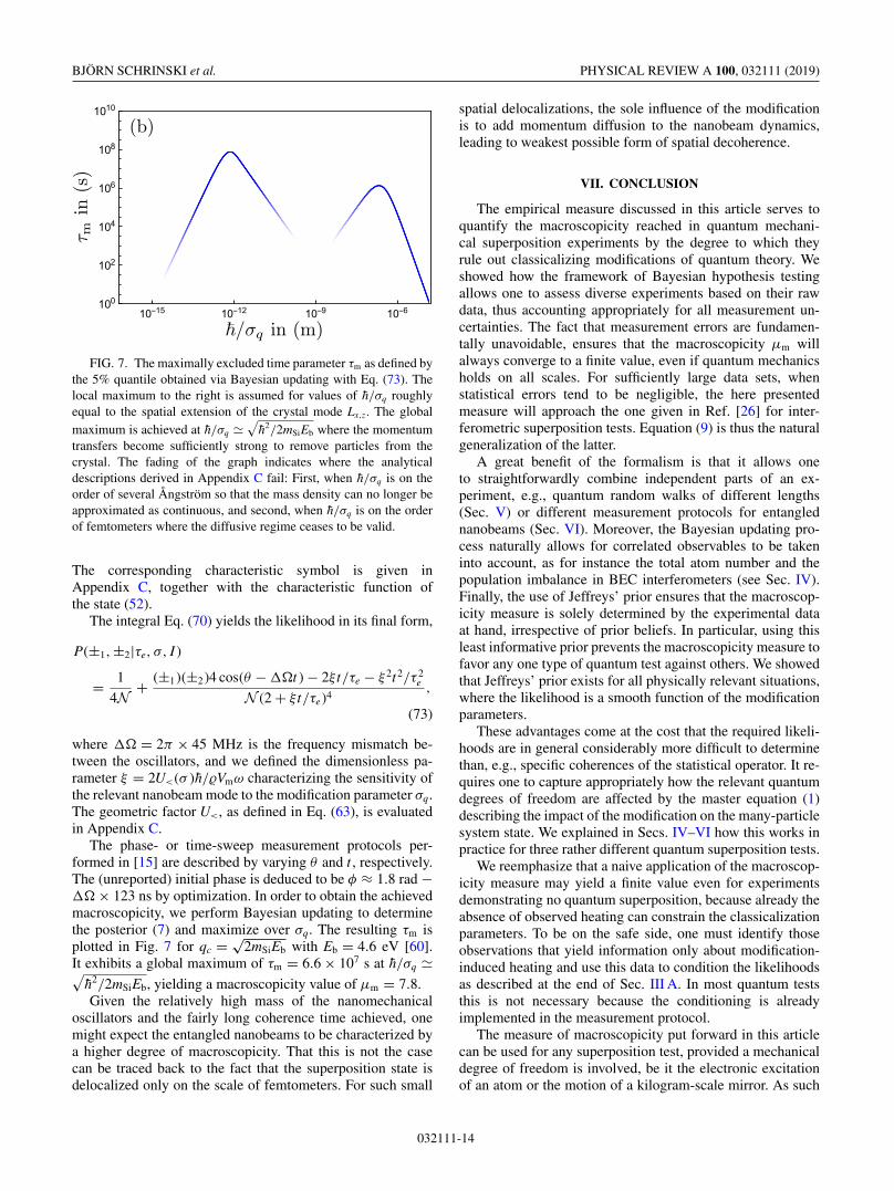
FIG. 7. The maximally excluded time parameter τm as defined bythe 5% quantile obtained via Bayesian updating with Eq. (73). Thelocal maximum to the right is assumed for values of h/σq roughlyequal to the spatial extension of the crystal mode Lx,z. The globalmaximum is achieved at h/σq �

√h2/2mSiEb where the momentum

transfers become sufficiently strong to remove particles from thecrystal. The fading of the graph indicates where the analyticaldescriptions derived in Appendix C fail: First, when h/σq is on theorder of several Ångström so that the mass density can no longer beapproximated as continuous, and second, when h/σq is on the orderof femtometers where the diffusive regime ceases to be valid.

The corresponding characteristic symbol is given inAppendix C, together with the characteristic function ofthe state (52).

The integral Eq. (70) yields the likelihood in its final form,

P(±1,±2|τe, σ, I )

= 1

4N + (±1)(±2)4 cos(θ − �t ) − 2ξ t/τe − ξ 2t2/τ 2e

N (2 + ξ t/τe)4,

(73)

where � = 2π × 45 MHz is the frequency mismatch be-tween the oscillators, and we defined the dimensionless pa-rameter ξ = 2U<(σ )h/�Vmω characterizing the sensitivity ofthe relevant nanobeam mode to the modification parameter σq.The geometric factor U<, as defined in Eq. (63), is evaluatedin Appendix C.

The phase- or time-sweep measurement protocols per-formed in [15] are described by varying θ and t , respectively.The (unreported) initial phase is deduced to be φ ≈ 1.8 rad −� × 123 ns by optimization. In order to obtain the achievedmacroscopicity, we perform Bayesian updating to determinethe posterior (7) and maximize over σq. The resulting τm isplotted in Fig. 7 for qc = √

2mSiEb with Eb = 4.6 eV [60].It exhibits a global maximum of τm = 6.6 × 107 s at h/σq �√

h2/2mSiEb, yielding a macroscopicity value of μm = 7.8.Given the relatively high mass of the nanomechanical

oscillators and the fairly long coherence time achieved, onemight expect the entangled nanobeams to be characterized bya higher degree of macroscopicity. That this is not the casecan be traced back to the fact that the superposition state isdelocalized only on the scale of femtometers. For such small

spatial delocalizations, the sole influence of the modificationis to add momentum diffusion to the nanobeam dynamics,leading to weakest possible form of spatial decoherence.

VII. CONCLUSION

The empirical measure discussed in this article serves toquantify the macroscopicity reached in quantum mechani-cal superposition experiments by the degree to which theyrule out classicalizing modifications of quantum theory. Weshowed how the framework of Bayesian hypothesis testingallows one to assess diverse experiments based on their rawdata, thus accounting appropriately for all measurement un-certainties. The fact that measurement errors are fundamen-tally unavoidable, ensures that the macroscopicity μm willalways converge to a finite value, even if quantum mechanicsholds on all scales. For sufficiently large data sets, whenstatistical errors tend to be negligible, the here presentedmeasure will approach the one given in Ref. [26] for inter-ferometric superposition tests. Equation (9) is thus the naturalgeneralization of the latter.

A great benefit of the formalism is that it allows oneto straightforwardly combine independent parts of an ex-periment, e.g., quantum random walks of different lengths(Sec. V) or different measurement protocols for entanglednanobeams (Sec. VI). Moreover, the Bayesian updating pro-cess naturally allows for correlated observables to be takeninto account, as for instance the total atom number and thepopulation imbalance in BEC interferometers (see Sec. IV).Finally, the use of Jeffreys’ prior ensures that the macroscop-icity measure is solely determined by the experimental dataat hand, irrespective of prior beliefs. In particular, using thisleast informative prior prevents the macroscopicity measure tofavor any one type of quantum test against others. We showedthat Jeffreys’ prior exists for all physically relevant situations,where the likelihood is a smooth function of the modificationparameters.

These advantages come at the cost that the required likeli-hoods are in general considerably more difficult to determinethan, e.g., specific coherences of the statistical operator. It re-quires one to capture appropriately how the relevant quantumdegrees of freedom are affected by the master equation (1)describing the impact of the modification on the many-particlesystem state. We explained in Secs. IV–VI how this works inpractice for three rather different quantum superposition tests.

We reemphasize that a naive application of the macroscop-icity measure may yield a finite value even for experimentsdemonstrating no quantum superposition, because already theabsence of observed heating can constrain the classicalizationparameters. To be on the safe side, one must identify thoseobservations that yield information only about modification-induced heating and use this data to condition the likelihoodsas described at the end of Sec. III A. In most quantum teststhis is not necessary because the conditioning is alreadyimplemented in the measurement protocol.

The measure of macroscopicity put forward in this articlecan be used for any superposition test, provided a mechanicaldegree of freedom is involved, be it the electronic excitationof an atom or the motion of a kilogram-scale mirror. As such

032111-14

MACROSCOPICITY OF QUANTUM MECHANICAL … PHYSICAL REVIEW A 100, 032111 (2019)

it does not apply to quantum tests involving only spins orphotons. It seems natural to generalize the macroscopicitymeasure to pure photon experiments by drawing on a minimalclass of classicalizing modifications of QED, but it is stillan open problem on how to get hold of the latter. Beyondthe assessment of macroscopicity, the Bayesian hypothesistesting presented in Sec. III, can also be used for a properstatistical description of tests of specific modification models,e.g., the various extensions of the continuous spontaneouslocalization model [2], but also of environmental decoherencemechanisms.

Finally, it goes without saying that the macroscopicity μm

attributed to a given superposition test serves to highlight asingle aspect of the experiment, albeit an important one. Itmust not be taken as a proxy for the overall significance of anexperimental finding.

ACKNOWLEDGMENTS

We thank Andrea Alberti, Tarik Berrada, and RalfRiedinger for helpful comments on their experiments, and theauthors of Ref. [15] for providing us with the unpublished rawdata reported in Fig. 4. B.S. thanks Gilles Kratzer for helpfuldiscussions on the topic of Bayesian statistics. This work wasfunded by Deutsche Forschungsgemeinschaft (DFG, GermanResearch Foundation), Grant No. 298796255.

APPENDIX A: INTEGRABILITY OF THEPOSTERIOR DISTRIBUTION

To see that Jeffreys’ prior (11) always yields a normalizableposterior distribution (7), we first consider the limit τe →∞, where the modification becomes arbitrarily weak. In thiscase the general solution of the master equation (1) can beexpanded to first order in 1/τe by its Dyson series. Calculatingthe likelihood then yields

P(D|τe, σ, I ) � P∞(D|I ) + 1

τeq(D|σ, I ) for τe → ∞,

(A1)

where q is independent of τe. Inserting the expansion (A1) intoJeffreys’ prior (11) yields

p(τe|σ, I )τe→∞∼

{τ−3/2

e ∃ d0 : P∞(d0|I ) = 0,

τ−2e else,

(A2)

implying that the posterior (7) decays at least as τ−3/2e for

τe → ∞.Second, for τe → 0, where modification-induced deco-

herence and heating get stronger and stronger, we use thatthe likelihood P(D|τe, σ, I ) will continuously approach somelimiting classical probability,

P(D|τe, σ, I ) � P0(D|σ, I ) + ταe q(D|σ, I ) for τe → 0,

(A3)

where α > 0 may depend on D. Using this to evaluate Jef-freys’ prior (11) yields that

p(τe|σ, I )τe→0∼

{τ−(1−αmin/2)

e ∃ d0 : P0(d0|σ, I ) = 0,

τ−(1−αmin )e else,

(A4)

where αmin > 0 is the minimal α. Physically speaking, thismeans that no quantum superposition test will support aclassical model of infinitely strong heating. Equation (A4)implies that the posterior always diverges weaker than 1/τe

for τe → 0.Finally, to rule out that the posterior diverges at a finite

τe ∈ (0,∞), we note that the likelihood P(D|τe, σ, I ) staysnon-negative for all τe. Thus, whenever it vanishes for somevalue of τe, its first derivative must also be zero and its secondderivative must be non-negative. Application of L’Hospital’srule then shows that the posterior stays finite for all inter-mediate values of τe. This completes the argument why thechoice of Jeffrey’s prior (11) always leads to a normaliz-able posterior (7) and thus yields a well-defined value ofmacroscopicity (9).

APPENDIX B: SIMULTANEOUS SHEARING ANDDIFFUSION OF NUMBER SQUEEZED BECs

For simultaneous phase diffusion and shearing the timeevolution of the tangent space Wigner function wt ( jy, jz ) isgiven by the equation

∂twt ( jy, jz ) = −( ε

h+ 2ζ jz

)∂ jywt ( jy, jz ) + �P

2∂2

jywt ( jy, jz ),

(B1)

which is solved by (24). If diffusion takes place perpendicularto the shearing, the time evolution is given by the equation

∂twt ( jy, jz ) = −2ζ jz∂ jywt ( jy, jz ) + �S

4∂2

jzwt ( jy, jz ), (B2)

without the free rotation around the general Bloch sphere thatcan be executed subsequently. Its general solution is

wt ( jy, jz ) = 1

4π2

∫d pyd pzd j′yd j′zw0( j′y, j′z )

× ei( jy−2ζ jzt )py−izpz−ipy j′y+ipz j′z

× exp

[−J2�S

(p2

z

4t − ζ py pz

2t2 − ζ 2 p2

y

3t3

)].

(B3)

We take the initial distribution w0( jy, jz ) to be a Gaussian withwidths σy and σz. Integrating jz preserves the Gaussian form,yielding the marginal distribution

wt ( jy) =∫

d jz wt ( jy, jz ) = 1√2πσ 2

y (t )exp

[j2y

2σ 2y (t )

],

(B4)

with variance

σ 2y (t ) = σ 2

y + 4ζ 2t2

(σ 2

z + J2�Lt

6

). (B5)

032111-15

BJÖRN SCHRINSKI et al. PHYSICAL REVIEW A 100, 032111 (2019)

APPENDIX C: CALCULATIONAL DETAILS FOR THE ENTANGLED NANOBEAMS EXPERIMENT

1. Normalization of displacement fields

The equation of motion of a classical displacement field in an isotropic elastic medium can be derived from the Lagrangiandensity [58]

L = �

2u2(r, t ) − V [u(r, t )]

= �

2u2 − 1

4

3∑klmn=1

(λ

2δklδmn + μδkmδln

)(∂uk

∂xl+ ∂ul

∂xk

)(∂um

∂xn+ ∂un

∂xm

), (C1)

where λ and μ are the Lamé coefficients. Thus, the dynamics of u(r, t ) are given by

�∂2u∂t2

= μ∇2u + (λ + μ)∇(∇ · u). (C2)

This equation can be solved by introducing the mode functions uk (r, t ) as the eigenfunctions of the differential operatoron the left-hand side with eigenvalues −ω2

k�. The total displacement field can then be written as

u(r, t ) =∑

k

√h

2ρVkωkwk (r)(e−iωkt ak + eiωkt a∗

k ), (C3)

so that its mean energy is

〈E〉t =⟨∫

d3r[�

2u2(r, t ) + V [u(r, t )]

]⟩t

=∑

k

hωk

Vk

∫d3r w2

k (r)a∗k ak . (C4)

Demanding that 〈E〉t =∑k hωka∗k ak yields the normalization condition

∫d3r w2

k (r) = Vk .

2. Characteristic functions of mechanical oscillator states

The characteristic function of the initial oscillator state in (52) for φ = 0 can be calculated as

χ±1 (Q, P) = 1

2exp

[− 1

4h�Vm

(P · �−1P + �2V 2

mQ · �Q)]

×⎛⎝1 − 1

4h�Vm

[∑λ=1,2

(±1)λ(�−1/2P)λ

]2

− �Vm

4h

[∑λ=1,2

(±1)λ(�1/2Q)λ

]2⎞⎠, (C5)

where � = diag(�1,�2). In a similar fashion, one obtains the characteristic symbols of the effect (72) as

η±2 (Q, P) = 1

2δ(Q)δ(P) −

[1 ±2 cos θ

(P1P2

h�Vm√

�1�2+ Q1Q2

�Vm√

�1�2

h

)±2 sin θ

(P1Q2

√�2

h2�1− P2Q1

√�1

h2�2

)]

× 1

8π2h2 exp

[− 1

4h�Vm

(P · �−1P + �2V 2

mQ · �Q)]

. (C6)

3. The geometric factor U<(σ )

Assuming a continuous mass density, valid if h/σq � 5 Å, the geometric factor (68) can be evaluated for the longitudinalmode (69) as

U<(σ ) � U (σ ) = 2�2h7

m2eσ

7q L3

z

(1 − e−L2

x σ 2q /2h2 +

√πLxσq√

2herf

[Lxσq√

2h

])2

×[√

2π

(h

[Lzσq

h, 0

]+ e−L2

z σ 2q /2h2

Re

{h

[Lzσq

h,

Lzσq

h

]})− (1 + e−L2

z σ 2q /2h2

)Lzσq

h

(π2 − 2

L2z σ

2q

h2

)],

(C7)

with

h[a, b] =√

π

2(i3a2 + πb2 − iπ2) exp

[(π/a − ib)2

2

]erf

[iπ/a + b√

2

]. (C8)

032111-16

MACROSCOPICITY OF QUANTUM MECHANICAL … PHYSICAL REVIEW A 100, 032111 (2019)

If h/σq is on the order of the lattice constant, the approximation of a continuous mass density fails. For even smaller h/σq theGaussian in (63) suppresses all contributions involving more than a single atom, so that the modification acts on each of the Natoms individually. The geometric factor then reads as

U<(σ ) = Nm2

Si

4h2m2e

erf

(qc√2σq

)2⎡⎣σ 2

q erf

(qc√2σq

)2

−√

2

πσqqce−q2

c /2σ 2q

⎤⎦. (C9)

Here we averaged the mode function (69) over the whole crystal∑

n w2(rn) ≈ N/2. As a result, the diffusion increasesquadratically with σq until the momentum displacements are strong enough to remove the particles from the crystal. In thelimit that σq qc one obtains U<(σ ) � Nm2

Siσ2q /4h2m2

e .

[1] A. J. Leggett, J. Phys. Condens. Matter 14, R415(2002).

[2] A. Bassi, K. Lochan, S. Satin, T. P. Singh, and H. Ulbricht, Rev.Mod. Phys. 85, 471 (2013).

[3] J. R. Friedman, V. Patel, W. Chen, S. Tolpygo, and J. E. Lukens,Nature (London) 406, 43 (2000).

[4] C. H. van der Wal, A. C. J. ter Haar, F. K. Wilhelm, R. N.Schouten, C. J. P. M. Harmans, T. P. Orlando, S. Lloyd, andJ. E. Mooij, Science 290, 773 (2000).

[5] A. Peters, K. Y. Chung, and S. Chu, Nature (London) 400, 849(1999).

[6] S. Dimopoulos, P. W. Graham, J. M. Hogan, and M. A.Kasevich, Phys. Rev. Lett. 98, 111102 (2007).

[7] S. Gerlich, S. Eibenberger, M. Tomandl, S. Nimmrichter, K.Hornberger, P. J. Fagan, J. Tüxen, M. Mayor, and M. Arndt,Nat. Commun. 2, 263 (2011).

[8] S. Eibenberger, S. Gerlich, M. Arndt, M. Mayor, and J. Tüxen,Phys. Chem. Chem. Phys. 15, 14696 (2013).

[9] T. Berrada, S. van Frank, R. Bücker, T. Schumm, J.-F. Schaff,and J. Schmiedmayer, Nat. Commun. 4, 2077 (2013).

[10] T. Kovachy, P. Asenbaum, C. Overstreet, C. A. Donnelly, S. M.Dickerson, A. Sugarbaker, J. M. Hogan, and M. A. Kasevich,Nature (London) 528, 530 (2015).

[11] A. Alberti, V. Ivanov, G. Tino, and G. Ferrari, Nat. Phys. 5, 547(2009).

[12] C. Robens, W. Alt, D. Meschede, C. Emary, and A. Alberti,Phys. Rev. X 5, 011003 (2015).

[13] P. Jurcevic, B. P. Lanyon, P. Hauke, C. Hempel, P. Zoller, R.Blatt, and C. F. Roos, Nature (London) 511, 202 (2014).

[14] R. Islam, R. Ma, P. M. Preiss, M. E. Tai, A. Lukin, M. Rispoli,and M. Greiner, Nature (London) 528, 77 (2015).

[15] R. Riedinger, A. Wallucks, I. Marinkovic, C. Löschnauer, M.Aspelmeyer, S. Hong, and S. Gröblacher, Nature (London) 556,473 (2018).

[16] C. Ockeloen-Korppi, E. Damskägg, J.-M. Pirkkalainen, M.Asjad, A. Clerk, F. Massel, M. Woolley, and M. Sillanpää,Nature (London) 556, 478 (2018).

[17] I. Marinkovic, A. Wallucks, R. Riedinger, S. Hong, M.Aspelmeyer, and S. Gröblacher, Phys. Rev. Lett. 121, 220404(2018).

[18] F. Fröwis, P. Sekatski, W. Dür, N. Gisin, and N. Sangouard, Rev.Mod. Phys. 90, 025004 (2018).

[19] J. I. Korsbakken, K. B. Whaley, J. Dubois, and J. I. Cirac, Phys.Rev. A 75, 042106 (2007).

[20] F. Marquardt, B. Abel, and J. von Delft, Phys. Rev. A 78,012109 (2008).

[21] F. Fröwis and W. Dür, New J. Phys. 14, 093039 (2012).[22] B. Yadin and V. Vedral, Phys. Rev. A 93, 022122 (2016).[23] B. Yadin, F. C. Binder, J. Thompson, V. Narasimhachar, M. Gu,

and M. S. Kim, Phys. Rev. X 8, 041038 (2018).[24] G. Björk and P. G. L. Mana, J. Opt. B 6, 429 (2004).[25] C.-W. Lee and H. Jeong, Phys. Rev. Lett. 106, 220401 (2011).[26] S. Nimmrichter and K. Hornberger, Phys. Rev. Lett. 110,

160403 (2013).[27] W. Von der Linden, V. Dose, and U. Von Toussaint, Bayesian

Probability Theory: Applications in the Physical Sciences (Cam-bridge University Press, Cambridge, 2014).

[28] L. Schwartz, Z. Wahrscheinlichkeitstheorie verw. Gebiete 4, 10(1965).

[29] J. Ghosh and R. Ramamoorthi, Springer Series in Statistics.Bayesian Nonparametrics (Springer, New York, 2003).

[30] F. Laloë, W. J. Mullin, and P. Pearle, Phys. Rev. A 90, 052119(2014).

[31] S. Nimmrichter, K. Hornberger, and K. Hammerer, Phys. Rev.Lett. 113, 020405 (2014).

[32] M. Carlesso, A. Bassi, P. Falferi, and A. Vinante, Phys. Rev. D94, 124036 (2016).

[33] J. Li, S. Zippilli, J. Zhang, and D. Vitali, Phys. Rev. A 93,050102(R) (2016).

[34] D. Goldwater, M. Paternostro, and P. F. Barker, Phys. Rev. A94, 010104(R) (2016).

[35] A. Vinante, R. Mezzena, P. Falferi, M. Carlesso, and A. Bassi,Phys. Rev. Lett. 119, 110401 (2017).

[36] B. Schrinski, B. A. Stickler, and K. Hornberger, J. Opt. Soc.Am. B 34, C1 (2017).

[37] S. L. Adler and A. Vinante, Phys. Rev. A 97, 052119 (2018).[38] M. Bahrami, Phys. Rev. A 97, 052118 (2018).[39] H. Jeffreys, The Theory of Probability (Oxford University Press,

Oxford, 1998).[40] J. M. Bernardo, J. Royal Stat. Soc. B 41, 113 (1979).[41] M. Ghosh et al., Stat. Sci. 26, 187 (2011).[42] J. O. Berger, J. M. Bernardo, D. Sun et al., Ann. Stat. 37, 905

(2009).[43] F. T. Arecchi, E. Courtens, R. Gilmore, and H. Thomas, Phys.

Rev. A 6, 2211 (1972).[44] M. Kitagawa and M. Ueda, Phys. Rev. A 47, 5138 (1993).[45] J. Ma, X. Wang, C. P. Sun, and F. Nori, Phys. Rep. 509, 89

(2011).

032111-17

BJÖRN SCHRINSKI et al. PHYSICAL REVIEW A 100, 032111 (2019)

[46] G. Tóth, Phys. Rev. A 85, 022322 (2012).[47] G. Tóth and I. Apellaniz, J. Phys. A 47, 424006 (2014).[48] O. Hosten, R. Krishnakumar, N. Engelsen, and M. Kasevich,

Science 352, 1552 (2016).[49] J. Javanainen and M. Wilkens, Phys. Rev. Lett. 78, 4675

(1997).[50] A. Sørensen, L.-M. Duan, J. Cirac, and P. Zoller, Nature

(London) 409, 63 (2001).[51] A. S. Sørensen and K. Mølmer, Phys. Rev. Lett. 86, 4431

(2001).[52] B. Lücke, J. Peise, G. Vitagliano, J. Arlt, L. Santos, G. Tóth,

and C. Klempt, Phys. Rev. Lett. 112, 155304 (2014).[53] M. Bilardello, A. Trombettoni, and A. Bassi, Phys. Rev. A 95,

032134 (2017).

[54] X. Wang, A. Miranowicz, Y. x. Liu, C. P. Sun, and F. Nori, Phys.Rev. A 81, 022106 (2010).

[55] S. van Frank, A. Negretti, T. Berrada, R. Bücker, S.Montangero, J.-F. Schaff, T. Schumm, T. Calarco, and J.Schmiedmayer, Nat. Commun. 5, 4009 (2014).

[56] B. Schrinski, K. Hornberger, and S. Nimmrichter, Quantum Sci.Technol. 2, 044010 (2017).

[57] O. Madelung, Introduction to Solid-State Theory (SpringerScience & Business Media, New York, 2012), Vol. 2.

[58] A. L. Fetter and J. D. Walecka, Theoretical Mechanics of Par-ticles and Continua (Courier Corporation, North Chelmsford,MA, 2003).

[59] R. Riedinger (private communication).[60] B. Farid and R. W. Godby, Phys. Rev. B 43, 14248 (1991).

032111-18