Physical principles of nanofiber production

Theoretical background (3)Electrical bi-layer

D. Lukáš2010

1

Electric bi-layer

2

Boltzmann equationPoisson EquationDebye‘s length

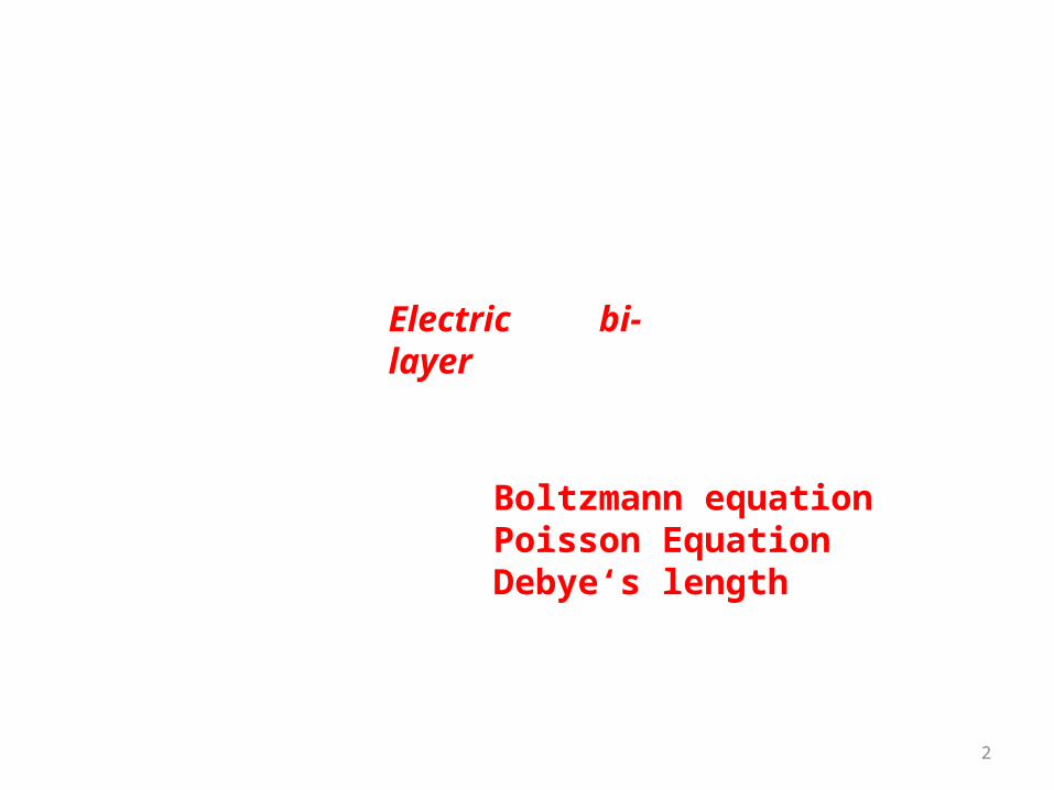
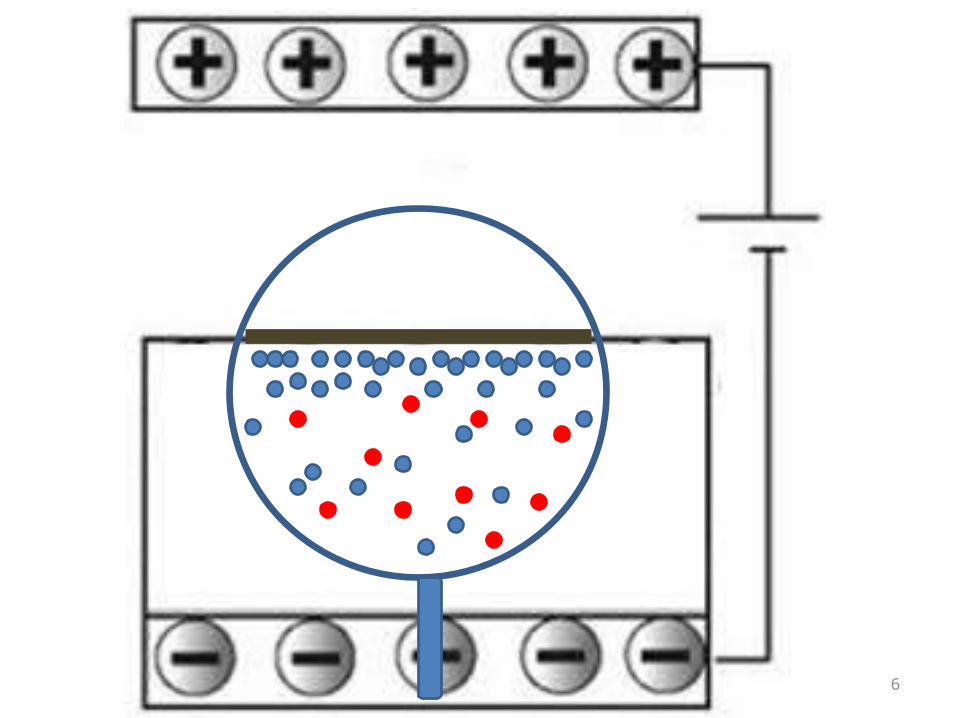
Electric bi-layer is another object with nano-dimension in electrospinning. Referring to second part of (Figure 3.2), one may consider a plane surface of polymer solution, containing ions both in polymer macromolecules and their solvent. Let the ion valence be considered as one for simplification and e denotes the elementary electric charge. In electrospinning, electric potential, 0, at the liquid / polymer solution surface is generated by the electrostatic field in between two electrodes.

Fig. 3.2:A cloud of ions (3) in a polymer solution (4) is induced by an electrostatic field between a collector (5) and an electrode (6). The thickness of the ionic atmosphere at the vicinity of the solution surface is called the ‘Debye’s length’, D.

3

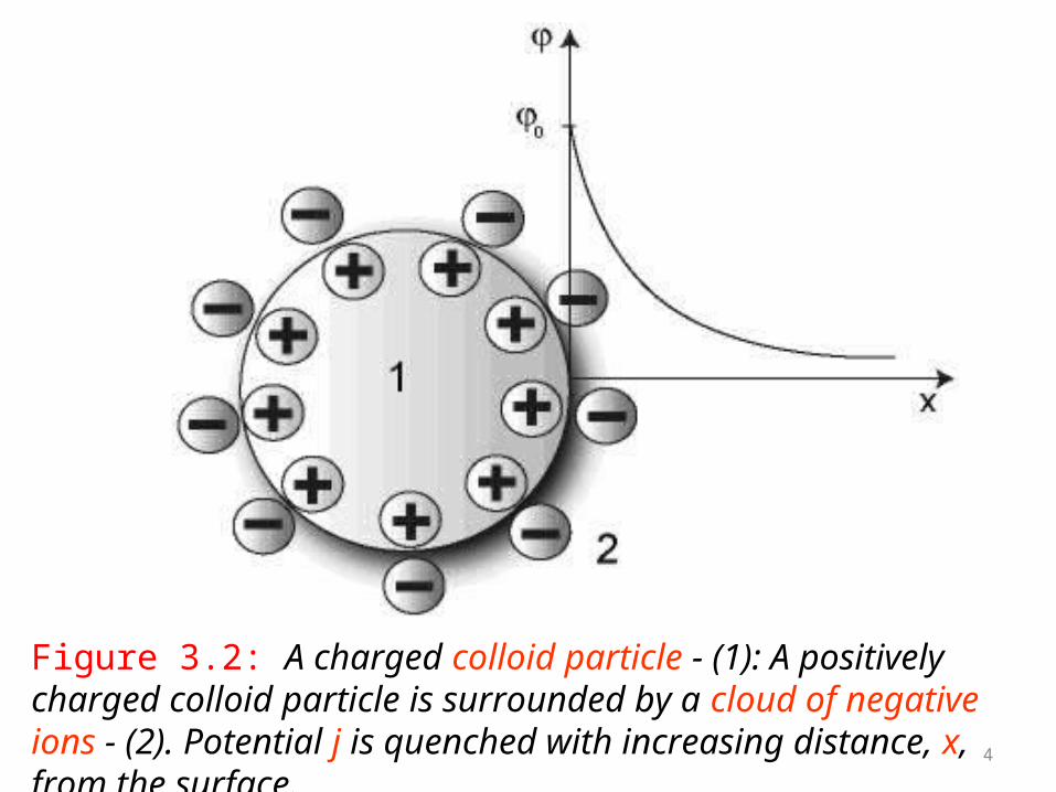
Figure 3.2: A charged colloid particle - (1): A positively charged colloid particle is surrounded by a cloud of negative ions - (2). Potential j is quenched with increasing distance, x, from the surface. 4

5

6

An electrospinner, from the point of view of ion distribution, resembles the situation in the vicinity of a charged colloid particle. The similitude is indicated in (Figure 3.2), where the collector plays the role of organised groups of charges on colloid particles. The only difference between colloid particle and electrospinner is the gap coined by the space between the collector and liquid surface.

7

++++ +

Prodleva!!!

8

D

‘Debye’s length‘

colloid particle

9

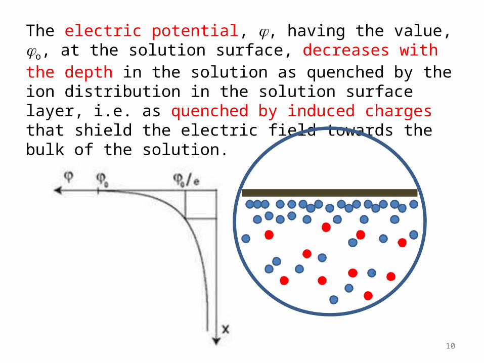
The electric potential, , having the value, o, at the solution surface, decreases with the depth in the solution as quenched by the ion distribution in the solution surface layer, i.e. as quenched by induced charges that shield the electric field towards the bulk of the solution.

10

For the sake of simplification relative parallel placement of both the collector and the solution surface will be considered henceforth. The parallel configuration gives rise to simple symmetric equipotential surfaces that are parallel to them too. So, the electrostatic potential (x) can be considered as the function of the only variable x, which is the distance measured along the axis, perpendicular to the collector and solution surfaces, with its origin located at the solution surface, pointing to the polymer solution bulk.

11

N

np )1(

N… Number of space cellsn… Number of particles

Configuration vector 1,0x

N

n

N

np

1)0,1(

)1,1(),1,0(),0,1(),0,0(x

Non-interacting free particles

12

Boltzmann equation

?)1( P

Tk

xExp

B

exp)( xexE

x

13

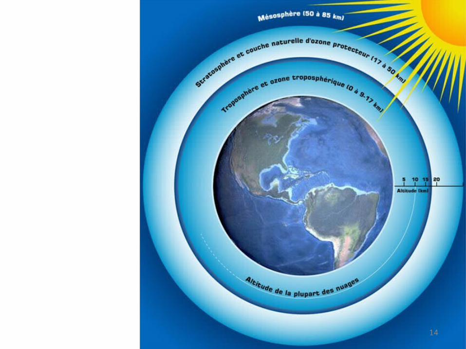
Analogie se zemskou atmosférou

14

kTmgxxp /exp)(

15

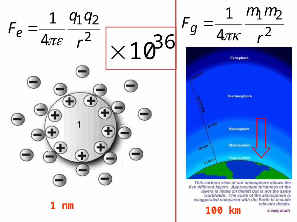
221

4

1

r

qqFe 2

21

4

1

r

mmFg

1 nm 100 km

3610

16

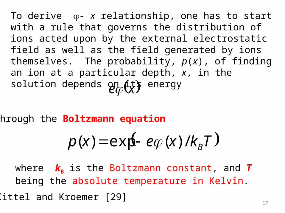
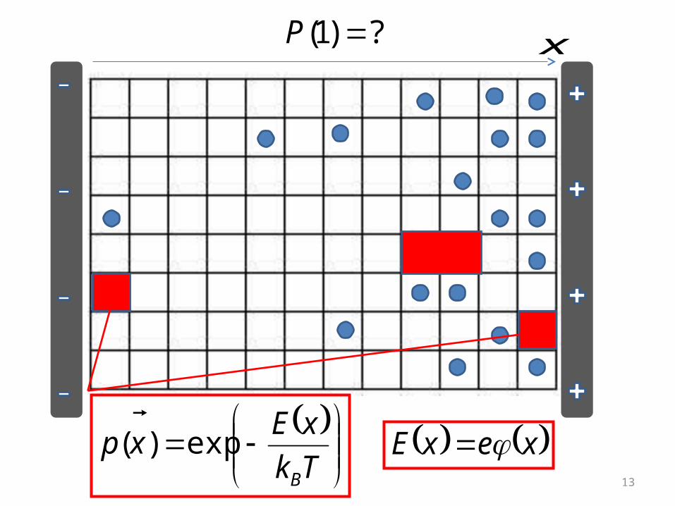
To derive - x relationship, one has to start with a rule that governs the distribution of ions acted upon by the external electrostatic field as well as the field generated by ions themselves. The probability, p(x), of finding an ion at a particular depth, x, in the solution depends on its energy

xe

through the Boltzmann equation

Tkxexp B/)(exp)(

where kB is the Boltzmann constant, and T being the absolute temperature in Kelvin.

Kittel and Kroemer [29]17

The electrolyte for this moment comprises two kinds of ions of opposite charge +e and –e. Their volumetric concentrations are:

Tkxenxn Bo /)(exp

Tkxenxn Bo /)(exp

Where n0 is the concentration of charges, when the solution is not affected by any external electrostatic field. The concentration n0 is universal for both the ions as the solution is electro-neutral as a whole.

onxnxnx 0)(

on

xnxp

)(

18

The charge distribution is also governed by the one-dimensional Maxwell’s first law of electrostatics, generally expressed in the form of Poisson Equation with the potential gradient

dxxd /)(having the nonzero component along the x axis only. Mathematically, the particular shape of the Equation (3.7) for this case becomes:

x

dx

xd

2

2

Tk

xe

Tk

xeenxenxenx

BBo

expexp

(3.10)

(3.11)Nonlinear differential equation!!!

19

Debye and Huckel [32] Linearization

Tk

xe

Tk

xeenx

BBo

expexp

Tk

xeen

Tk

xe

Tk

xeenxTkxe

Bo

BBoB

11

.....!4!3!2!1

1.....,!4!3!2!1

1432432

xxxxe

xxxxe xx

xexex xx 1,11

Tk

xen

dx

xd

Bo 2

2

2

220

xTk

en

dx

xd

B

o

2

2

2 2

Debye and Huckel [32] Linearization

012 2

2 Tk

en

B

o

Tk

en

B

o

22

1,,22

2

xdx

xd

dx

xd

x

Tk

eneCx

B

x

20

0

2exp

21

‘Debye’s length‘

D

xx

Tk

enx

B

exp2

exp 0

20

0

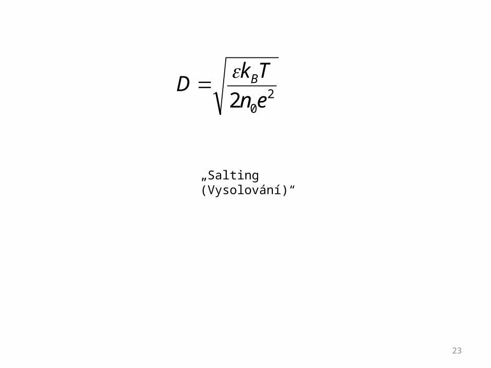
202 en

TkD B

D D

22

several units or tens of nanometres

23

202 en

TkD B

„Salting (Vysolování)“

0E

E

+

Conductive body (liquid body)

Intensity inside conductive body is zero.

Intensity vectors (on the surface of conductive body) are perpendicular to body surface.

Surface of body is equipotentials. 24

25

Electric layer

+

-

26

With respect to electrospinning, one can underline that Debye’s length is the thickness of the ion cloud at the vicinity of the liquid surface.

As this thickness in conductive liquids is generally not more than several units or tens of nanometres, the external electrostatic field is able to influence directly only the molecules that are close to the liquid surface.

It is convenient to underline on this place that the electrostatic field grasps during electrospinning preferably the surface layer of the liquid where net charges are enormously concentrated.

The surface husk of the liquid is transmitted into a jet that is hence supposed to be highly charged too.

27